
Digital Modulation 1 - Department of Electronic...
199
Digital Modulation 1 – Lecture Notes – Ingmar Land and Bernard H. Fleury Navigation and Communications (NavCom) Department of Electronic Systems Aalborg University, DK Version: February 5, 2007
Transcript of Digital Modulation 1 - Department of Electronic...

Digital Modulation 1– Lecture Notes –
Ingmar Land and Bernard H. Fleury
Navigation and Communications (NavCom)
Department of Electronic Systems
Aalborg University, DK
Version: February 5, 2007

i
Contents
I Basic Concepts 1
1 The Basic Constituents of a Digital Communication System 2
1.1 Discrete Information Sources . . . . . . . . . . . . 4
1.2 Considered System Model . . . . . . . . . . . . . . 6
1.3 The Digital Transmitter . . . . . . . . . . . . . . . 10
1.3.1 Waveform Look-up Table . . . . . . . . . . 10
1.3.2 Waveform Synthesis . . . . . . . . . . . . . 12
1.3.3 Canonical Decomposition . . . . . . . . . . 13
1.4 The Additive White Gaussian-Noise Channel . . . . 15
1.5 The Digital Receiver . . . . . . . . . . . . . . . . . 17
1.5.1 Bank of Correlators . . . . . . . . . . . . . 17
1.5.2 Canonical Decomposition . . . . . . . . . . 18
1.5.3 Analysis of the correlator outputs . . . . . . 20
1.5.4 Statistical Properties of the Noise Vector . . 23
1.6 The AWGN Vector Channel . . . . . . . . . . . . . 27
1.7 Vector Representation of a Digital Communication System 28
1.8 Signal-to-Noise Ratio for the AWGN Channel . . . 31
2 Optimum Decoding for the AWGN Channel 33
2.1 Optimality Criterion . . . . . . . . . . . . . . . . . 33
2.2 Decision Rules . . . . . . . . . . . . . . . . . . . . 34
2.3 Decision Regions . . . . . . . . . . . . . . . . . . . 36
Land, Fleury: Digital Modulation 1 NavCom
ii
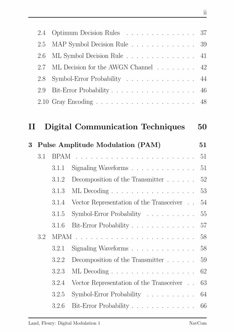
2.4 Optimum Decision Rules . . . . . . . . . . . . . . 37
2.5 MAP Symbol Decision Rule . . . . . . . . . . . . . 39
2.6 ML Symbol Decision Rule . . . . . . . . . . . . . . 41
2.7 ML Decision for the AWGN Channel . . . . . . . . 42
2.8 Symbol-Error Probability . . . . . . . . . . . . . . 44
2.9 Bit-Error Probability . . . . . . . . . . . . . . . . . 46
2.10 Gray Encoding . . . . . . . . . . . . . . . . . . . . 48
II Digital Communication Techniques 50
3 Pulse Amplitude Modulation (PAM) 51
3.1 BPAM . . . . . . . . . . . . . . . . . . . . . . . . 51
3.1.1 Signaling Waveforms . . . . . . . . . . . . . 51
3.1.2 Decomposition of the Transmitter . . . . . . 52
3.1.3 ML Decoding . . . . . . . . . . . . . . . . . 53
3.1.4 Vector Representation of the Transceiver . . 54
3.1.5 Symbol-Error Probability . . . . . . . . . . 55
3.1.6 Bit-Error Probability . . . . . . . . . . . . . 57
3.2 MPAM . . . . . . . . . . . . . . . . . . . . . . . . 58
3.2.1 Signaling Waveforms . . . . . . . . . . . . . 58
3.2.2 Decomposition of the Transmitter . . . . . . 59
3.2.3 ML Decoding . . . . . . . . . . . . . . . . . 62
3.2.4 Vector Representation of the Transceiver . . 63
3.2.5 Symbol-Error Probability . . . . . . . . . . 64
3.2.6 Bit-Error Probability . . . . . . . . . . . . . 66
Land, Fleury: Digital Modulation 1 NavCom

iii
4 Pulse Position Modulation (PPM) 67
4.1 BPPM . . . . . . . . . . . . . . . . . . . . . . . . 67
4.1.1 Signaling Waveforms . . . . . . . . . . . . . 67
4.1.2 Decomposition of the Transmitter . . . . . . 68
4.1.3 ML Decoding . . . . . . . . . . . . . . . . . 69
4.1.4 Vector Representation of the Transceiver . . 71
4.1.5 Symbol-Error Probability . . . . . . . . . . 72
4.1.6 Bit-Error Probability . . . . . . . . . . . . . 73
4.2 MPPM . . . . . . . . . . . . . . . . . . . . . . . . 74
4.2.1 Signaling Waveforms . . . . . . . . . . . . . 74
4.2.2 Decomposition of the Transmitter . . . . . . 75
4.2.3 ML Decoding . . . . . . . . . . . . . . . . . 77
4.2.4 Symbol-Error Probability . . . . . . . . . . 78
4.2.5 Bit-Error Probability . . . . . . . . . . . . . 80
5 Phase-Shift Keying (PSK) 85
5.1 Signaling Waveforms . . . . . . . . . . . . . . . . . 85
5.2 Signal Constellation . . . . . . . . . . . . . . . . . 87
5.3 ML Decoding . . . . . . . . . . . . . . . . . . . . . 90
5.4 Vector Representation of the MPSK Transceiver . . 93
5.5 Symbol-Error Probability . . . . . . . . . . . . . . 94
5.6 Bit-Error Probability . . . . . . . . . . . . . . . . . 97
6 Offset Quadrature Phase-Shift Keying (OQPSK)100
6.1 Signaling Scheme . . . . . . . . . . . . . . . . . . . 100
6.2 Transceiver . . . . . . . . . . . . . . . . . . . . . . 101
6.3 Phase Transitions for QPSK and OQPSK . . . . . 102
Land, Fleury: Digital Modulation 1 NavCom

iv
7 Frequency-Shift Keying (FSK) 104
7.1 BFSK with Coherent Demodulation . . . . . . . . . 104
7.1.1 Signal Waveforms . . . . . . . . . . . . . . 104
7.1.2 Signal Constellation . . . . . . . . . . . . . 106
7.1.3 ML Decoding . . . . . . . . . . . . . . . . . 107
7.1.4 Vector Representation of the Transceiver . . 108
7.1.5 Error Probabilities . . . . . . . . . . . . . . 109
7.2 MFSK with Coherent Demodulation . . . . . . . . 110
7.2.1 Signal Waveforms . . . . . . . . . . . . . . 110
7.2.2 Signal Constellation . . . . . . . . . . . . . 111
7.2.3 Vector Representation of the Transceiver . . 112
7.2.4 Error Probabilities . . . . . . . . . . . . . . 113
7.3 BFSK with Noncoherent Demodulation . . . . . . . 114
7.3.1 Signal Waveforms . . . . . . . . . . . . . . 114
7.3.2 Signal Constellation . . . . . . . . . . . . . 115
7.3.3 Noncoherent Demodulator . . . . . . . . . . 116
7.3.4 Conditional Probability of Received Vector . 117
7.3.5 ML Decoding . . . . . . . . . . . . . . . . . 119
7.4 MFSK with Noncoherent Demodulation . . . . . . 121
7.4.1 Signal Waveforms . . . . . . . . . . . . . . 121
7.4.2 Signal Constellation . . . . . . . . . . . . . 122
7.4.3 Conditional Probability of Received Vector . 123
7.4.4 ML Decision Rule . . . . . . . . . . . . . . 123
7.4.5 Optimal Noncoherent Receiver for MFSK . . 124
7.4.6 Symbol-Error Probability . . . . . . . . . . 125
7.4.7 Bit-Error Probability . . . . . . . . . . . . . 129
Land, Fleury: Digital Modulation 1 NavCom

v
8 Minimum-Shift Keying (MSK) 130
8.1 Motivation . . . . . . . . . . . . . . . . . . . . . . 130
8.2 Transmit Signal . . . . . . . . . . . . . . . . . . . 132
8.3 Signal Constellation . . . . . . . . . . . . . . . . . 135
8.4 A Finite-State Machine . . . . . . . . . . . . . . . 138
8.5 Vector Encoder . . . . . . . . . . . . . . . . . . . 140
8.6 Demodulator . . . . . . . . . . . . . . . . . . . . . 144
8.7 Conditional Probability Density of Received Sequence145
8.8 ML Sequence Estimation . . . . . . . . . . . . . . 146
8.9 Canonical Decomposition of MSK . . . . . . . . . . 149
8.10 The Viterbi Algorithm . . . . . . . . . . . . . . . . 150
8.11 Simplified ML Decoder . . . . . . . . . . . . . . . 155
8.12 Bit-Error Probability . . . . . . . . . . . . . . . . . 160
8.13 Differential Encoding and Differential Decoding . . 161
8.14 Precoded MSK . . . . . . . . . . . . . . . . . . . . 162
8.15 Gaussian MSK . . . . . . . . . . . . . . . . . . . . 166
9 Quadrature Amplitude Modulation 169
10 BPAM with Bandlimited Waveforms 170
III Appendix 171
Land, Fleury: Digital Modulation 1 NavCom

vi
A Geometrical Representation of Signals 172
A.1 Sets of Orthonormal Functions . . . . . . . . . . . 172
A.2 Signal Space Spanned by an Orthonormal Set of Functions173
A.3 Vector Representation of Elements in the Vector Space174
A.4 Vector Isomorphism . . . . . . . . . . . . . . . . . 175
A.5 Scalar Product and Isometry . . . . . . . . . . . . 176
A.6 Waveform Synthesis . . . . . . . . . . . . . . . . . 178
A.7 Implementation of the Scalar Product . . . . . . . . 179
A.8 Computation of the Vector Representation . . . . . 181
A.9 Gram-Schmidt Orthonormalization . . . . . . . . . 182
B Orthogonal Transformation of a White Gaussian Noise Vector 185
B.1 The Two-Dimensional Case . . . . . . . . . . . . . 185
B.2 The General Case . . . . . . . . . . . . . . . . . . 186
C The Shannon Limit 188
C.1 Capacity of the Band-limited AWGN Channel . . . 188
C.2 Capacity of the Band-Unlimited AWGN Channel . 191
Land, Fleury: Digital Modulation 1 NavCom

vii
References
[1] J. G. Proakis and M. Salehi, Communication Systems Engi-
neering, 2nd ed. Prentice-Hall, 2002.
[2] B. Rimoldi, “A decomposition approach to CPM,” IEEE
Trans. Inform. Theory, vol. 34, no. 2, pp. 260–270, Mar. 1988.
Land, Fleury: Digital Modulation 1 NavCom

1
Part I
Basic Concepts
Land, Fleury: Digital Modulation 1 NavCom
2
1 The Basic Constituents of a Digi-tal Communication System
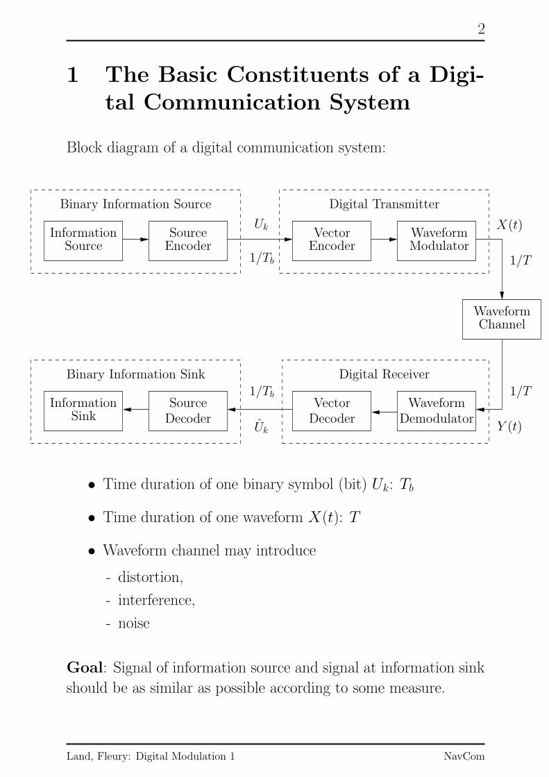
Block diagram of a digital communication system:
PSfrag replacements
Binary Information Source
Binary Information Sink
Digital Transmitter
Digital Receiver
Information
Information
Source
SourceSource
Encoder EncoderVector
Vector
Waveform
Waveform
Waveform
Modulator
Channel
Decoder Decoder DemodulatorSink
Uk
Uk
X(t)
Y (t)
1/Tb
1/Tb
1/T
1/T
• Time duration of one binary symbol (bit) Uk: Tb
• Time duration of one waveform X(t): T
• Waveform channel may introduce
- distortion,
- interference,
- noise
Goal: Signal of information source and signal at information sink
should be as similar as possible according to some measure.
Land, Fleury: Digital Modulation 1 NavCom

3
Some properties:
• Information source: may be analog or digital
• Source encoder: may perform sampling, quantization and
compression; generates one binary symbol (bit) Uk ∈ {0, 1}per time interval Tb
• Waveform modulator: generates one waveform x(t) per time
interval T
• Vector decoder: generates one binary symbol (bit) Uk ∈{0, 1} (estimates of Uk) per time interval Tb
• Source decoder: reconstructs the original source signal
Land, Fleury: Digital Modulation 1 NavCom

4
1.1 Discrete Information Sources
A discrete memoryless source (DMS) is a source that generates
a sequence U1, U2, . . . of independent and identically distributed
(i.i.d.) discrete random variables, called an i.i.d. sequence.
PSfrag replacements
DMS U1, U2, . . .
Properties of the output sequence:
discrete U1, U2, . . . ∈ {a1, a2, . . . , aQ}.
memoryless U1, U2, . . . are statistically independent.
stationary U1, U2, . . . are identically distributed.
Notice: The symbol alphabet {a1, a2, . . . , aQ} has cardinality Q.
The value of Q may be infinite, the elements of the alphabet only
have to be countable.
Example: Discrete sources
(i) Output of the PC keyboard, SMS
(usually not memoryless).
(ii) Compressed file
(near memoryless).
(iii) The numbers drawn on a roulette table in a casino
(ought to be memoryless, but may not. . . ).
3
Land, Fleury: Digital Modulation 1 NavCom

5
A DMS is statistically completely described by the probabilities
pU(aq) = Pr(U = aq)
of the symbols aq, q = 1, 2, . . . , Q. Notice that
(i) pU(aq) ≥ 0 for all q = 1, 2, . . . , Q, and
(ii)
Q∑
q=1
pU(aq) = 1.
As the sequence is i.i.d., we have Pr(Ui = aq) = Pr(Uj = aq).
For convenience, we may write pU(a) shortly as p(a).
Binary Symmetric Source
A binary memoryless source is a DMS with a binary symbol al-
phabet.
Remark:
Commonly used binary symbol alphabets are F2 := {0, 1} and
B := {−1,+1}. In the following, we will use F2.
A binary symmetric source (BSS) is a binary memoryless source
with equiprobable symbols,
pU(0) = pU(1) =1
2.
Example: Binary Symmetric Source
All length-K sequences of a BSS have the same probability
pU1U2...UK(u1u2 . . . uK) =
K∏
i=1
pU(ui) =(1
2
)K
.
3
Land, Fleury: Digital Modulation 1 NavCom

6
1.2 Considered System Model
This course focuses on the transmitter and the receiver. Therefore,
we replace the information source by a BSS
PSfrag replacements
BSS
Binary
Information SourceSource Encoder
DecoderSink
U1, U2, . . .
U1, U2, . . .
and the information sink by a binary (information) sink.
PSfrag replacements
BSS
Binary
Information Source
Encoder
Decoder
Sink
Sink
U1, U2, . . . U1, U2, . . .
U1, U2, . . .
Land, Fleury: Digital Modulation 1 NavCom

7
Some Remarks
(i) There is no loss of generality resulting from these substitutions.
Indeed it can be demonstrated within Shannon’s Information The-
ory that an efficient source encoder converts the output of an in-
formation source into a random binary independent and uniformly
distributed (i.u.d.) sequence. Thus, the output of a perfect source
encoder looks like the output of a BSS.
(ii) Our main concern is the design of communication systems for
reliable transmission of the output symbols of a BSS. We will not
address the various methods for efficient source encoding.
Land, Fleury: Digital Modulation 1 NavCom

8
Digital communication system considered in this course:
PSfrag replacements
BSS
BinarySink
Digital
DigitalTransmitter
Receiver
WaveformChannel
U
U
X(t)
Y (t)
bit rate 1/Tb rate 1/T
• Source: U = [U1, . . . , UK ], Ui ∈ {0, 1}
• Transmitter: X(t) = x(t,u)
• Sink: U = [U1, . . . , UK ], Ui ∈ {0, 1}
• Bit rate: 1/Tb
• Rate (of waveforms): 1/T = 1/(KTb)
• Bit error probability
Pb =1
K
K∑
k=1
Pr(Uk 6= Uk)
Objective: Design of efficient digital communication systems
Efficiency means
{
small bit error probability and
high bit rate 1/Tb.
Land, Fleury: Digital Modulation 1 NavCom

9
Constraints and limitations:
• limited power
• limited bandwidth
• impairments (distortion, interference, noise) of the channel
Design goals:
• “good” waveforms
• low-complexity transmitters
• low-complexity receivers
Land, Fleury: Digital Modulation 1 NavCom

10
1.3 The Digital Transmitter
1.3.1 Waveform Look-up Table
Example: 4PPM (Pulse-Position Modulation)
Set of four different waveforms, S = {s1(t), s2(t), s3(t), s4(t)}:PSfrag replacements
00
T
A
t
s1(t)
PSfrag replacements
00
T
A
ts1(t)
s2(t)
PSfrag replacements
00
T
A
t
s1(t)
s2(t)
s3(t)
PSfrag replacements
00
T
A
t
s1(t)
s2(t)
s3(t)
s4(t)
Each waveform X(t) ∈ S is addressed by vector [U1, U2] ∈ {0, 1}2:[U1, U2] 7→ X(t).
The mapping may be implemented by a waveform look-up table.PSfrag replacements
4PPMTransmitter
[U1, U2] X(t)[00] 7→ s1(t)[01] 7→ s2(t)
[10] 7→ s3(t)[11] 7→ s4(t)
Example: [00011100] is transmitted as
PSfrag replacements
00
T 2T 3T 4T
A
t
x(t)
3
Land, Fleury: Digital Modulation 1 NavCom

11
For an arbitrary digital transmitter, we have the following:PSfrag replacements
DigitalTransmitter
WaveformLook-upTable
[U1, U2, . . . , UK ] X(t)
Input Binary vectors of length K from the input set U:
[U1, U2, . . . , UK ] ∈ U := {0, 1}K.The “duration” of one binary symbol Uk is Tb.
Output Waveforms of duration T from the output set S:
x(t) ∈ S := {s1(t), s2(t), . . . , sM(t)}.Waveform duration T means that for m = 1, 2, . . . ,M ,
sm(t) = 0 for t /∈ [0, T ].
The look-up table maps each input vector [u1, . . . , uK ] ∈ U to one
waveform x(t) ∈ S. Thus the digital transmitter may defined by
a mapping U→ S with
[u1, . . . , uK ] 7→ x(t).
The mapping is one-to-one and onto such that
M = 2K.
Relation between signaling interval (waveform duration) T and bit
interval (“bit duration”) Tb:
T = K · Tb.
Land, Fleury: Digital Modulation 1 NavCom

12
1.3.2 Waveform Synthesis
The set of waveforms,
S := {s1(t), s2(t), . . . , sM(t)},
spans a vector space. Applying the Gram-Schmidt orthogonaliza-
tion procedure, we can find a set of orthonormal functions
Sψ := {ψ1(t), ψ2(t), . . . , ψD(t)} with D ≤M
such that the space spanned by Sψ contains the space spanned
by S.
Hence, each waveform sm(t) can be represented by a linear combi-
nation of the orthonormal functions:
sm(t) =
D∑
i=1
sm,i · ψi(t),
m = 1, 2, . . . ,M . Each signal sm(t) can thus be geometrically
represented by the D-dimensional vector
sm = [sm,1, sm,2, . . . , sm,D]T ∈ RD
with respect to the set Sψ.
Further details are given in Appendix A.
Land, Fleury: Digital Modulation 1 NavCom

13
1.3.3 Canonical Decomposition
The digital transmitter may be represented by a waveform look-up
table:
u = [u1, . . . , uK ] 7→ x(t),
where u ∈ U and x(t) ∈ S.
From the previous section, we know how to synthesize the wave-
form sm(t) from sm (see also Appendix A) with respect to a set of
basis functions
Sψ := {ψ1(t), ψ2(t), . . . , ψD(t)}.Making use of this method, we can split the waveform look-up
table into a vector look-up table and a waveform synthesizer:
u = [u1, . . . , uK ] 7→ x = [x1, x2, . . . , xD] 7→ x(t),
where
u ∈ U = {0, 1}K,x ∈ X = {s1, s2, . . . , sD} ⊂ R
D,
x(t) ∈ S = {s1(t), s2(t), . . . , sM(t)}.
This splitting procedure leads to the sought canonical decomposi-
tion of a digital transmitter:
PSfrag replacements
Vector
VectorEncoder
WaveformModulator
Look-up Table[U1, . . . , UK ]
X1
XD
ψ1(t)
ψD(t)
X(t)[0 . . . 0] 7→ s1
[1 . . . 1] 7→ sM
Land, Fleury: Digital Modulation 1 NavCom
14
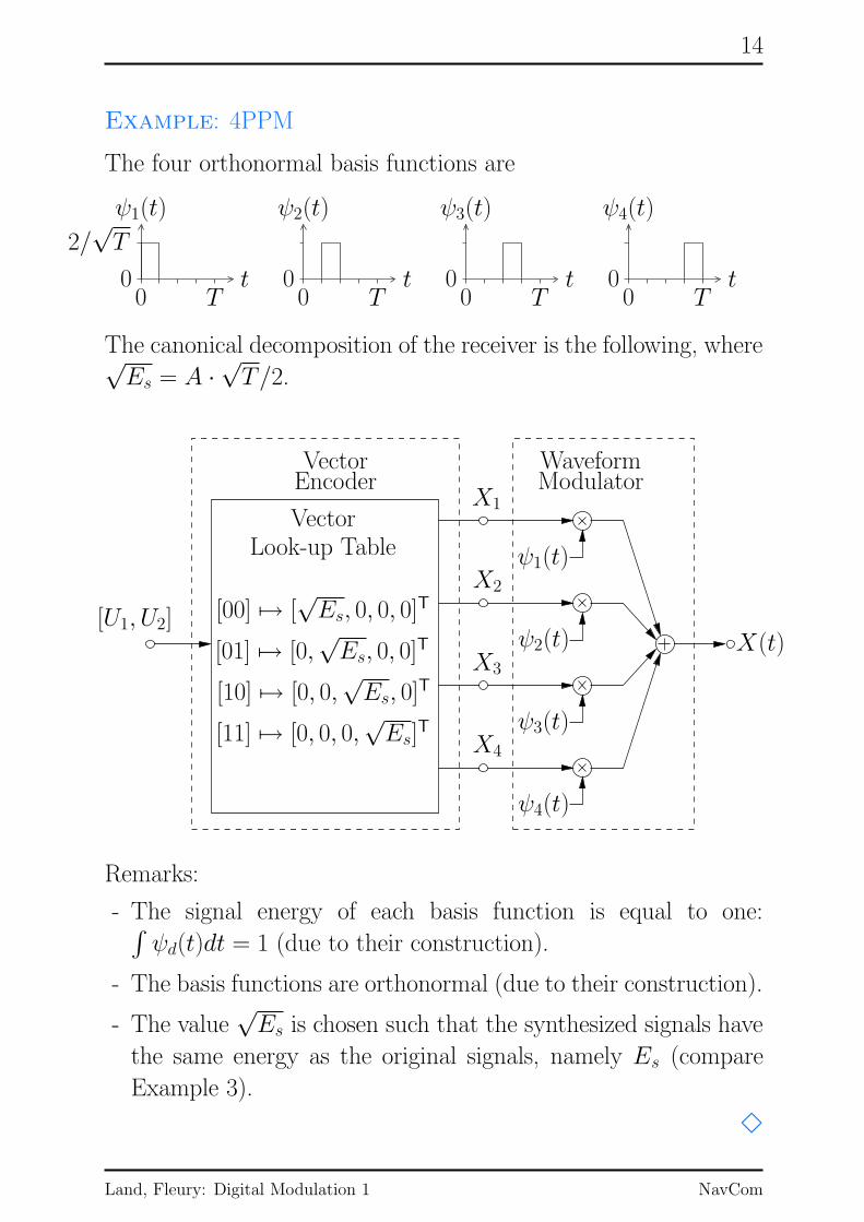
Example: 4PPM
The four orthonormal basis functions are
PSfrag replacements
00
T
2/√T
t
ψ1(t)
PSfrag replacements
00
T
2/√T
t
ψ1(t)ψ2(t)
PSfrag replacements
00
T
2/√T
t
ψ1(t)
ψ2(t)
ψ3(t)
PSfrag replacements
00
T
2/√T
t
ψ1(t)
ψ2(t)
ψ3(t)
ψ4(t)
The canonical decomposition of the receiver is the following, where√Es = A ·
√T/2.
PSfrag replacements
Vector Encoder
Vector
Encoder
Waveform Modulator
WaveformModulator
Vector
VectorLook-up Table
[U1, U2]
X1
X2
X3
X4
ψ1(t)
ψ2(t)
ψ3(t)
ψ4(t)
X(t)
[00] 7→ [√Es, 0, 0, 0]T
[01] 7→ [0,√Es, 0, 0]T
[10] 7→ [0, 0,√Es, 0]T
[11] 7→ [0, 0, 0,√Es]
T
Remarks:
- The signal energy of each basis function is equal to one:∫ψd(t)dt = 1 (due to their construction).
- The basis functions are orthonormal (due to their construction).
- The value√Es is chosen such that the synthesized signals have
the same energy as the original signals, namely Es (compare
Example 3).
3
Land, Fleury: Digital Modulation 1 NavCom

15
1.4 The Additive White Gaussian-NoiseChannel
PSfrag replacements
X(t) Y (t)
W (t)
The additive white Gaussian noise (AWGN) channel-model is
widely used in communications. The transmitted signal X(t) is
superimposed by a stochastic noise signal W (t), such that the
transmitted signal reads
Y (t) = X(t) +W (t).
The stochastic process W (t) is a stationary process with the
following properties:
(i) W (t) is a Gaussian process, i.e., for each time t, the
samples v = w(t) are Gaussian distributed with zero mean
and variance σ2:
pV (v) =1√
2πσ2exp(− v2
2σ2
).
(ii) W (t) has a flat power spectrum with height N0/2:
SW (f ) =N0
2
(Therefore it is called “white”.)
(iii) W (t) has the autocorrelation function
RW (τ ) =N0
2δ(τ ).
Land, Fleury: Digital Modulation 1 NavCom

16
Remarks
1. Autocorrelation function and power spectrum:
RW (τ ) = E[W (t)W (t + τ )
], SW (f ) = F
{RW (τ )
}.
2. For Gaussian processes, weak stationarity implies strong sta-
tionarity.
3. An WGN is an idealized process without physical reality:
• The process is so “wild” that its realizations are not
ordinary functions of time.
• Its power is infinite.
However, a WGN is a useful approximation of a noise with a
flat power spectrum in the bandwidth B used by a commu-
nication system:
PSfrag replacements Snoise(f )
N0/2
ff0−f0
BB
4. In satellite communications, W (t) is the thermal noise of the
receiver front-end. In this case, N0/2 is proportional to the
squared temperature.
Land, Fleury: Digital Modulation 1 NavCom

17
1.5 The Digital Receiver
Consider a transmission system using the waveforms
S ={
s1(t), s2(t), . . . , sM(t)}
with sm(t) = 0 for t /∈ [0, T ], m = 1, 2, . . . ,M , i.e., with dura-
tion T .
Assume transmission over an AWGN channel, such that
y(t) = x(t) + w(t),
x(t) ∈ S.
1.5.1 Bank of Correlators
The transmitted waveform may be recovered from the received
waveform y(t) by correlating y(t) with all possible waveforms:
cm = 〈y(t), sm(t)〉,
m = 1, 2, . . . ,M . Based on the correlations [c1, . . . , cM ], the wave-
form s(t) with the highest correlation is chosen and the correspond-
ing (estimated) source vector u = [u1, . . . , uK ] is output.
PSfrag replacements
y(t)s1(t)
sM(t)
∫ T
0 (.)dt
∫ T
0 (.)dtc1
cM
estimationof x(t)
andtable
look-up
[u1, . . . , uK ]
Disadvantage: High complexity.
Land, Fleury: Digital Modulation 1 NavCom

18
1.5.2 Canonical Decomposition
Consider a set of orthonormal functions
Sψ ={
ψ1(t), ψ2(t), . . . , ψD(t)}
obtained by applying the Gram-Schmidt procedure to
s1(t), s2(t), . . . , sM(t). Then,
sm(t) =
D∑
d=1
sm,d · ψd(t),
m = 1, 2, . . . ,M . The vector
sm = [sm,1, sm,2, . . . , sm,D]T
entirely determines sm(t) with respect to the orthonormal set Sψ.
The set Sψ spans the vector space
Sψ :={
s(t) =
D∑
i=1
siψi(t) : [s1, s2, . . . , sD] ∈ RD}
.
Basic Idea
• The received waveform y(t) may contain components outside
of Sψ. However, only the components inside Sψ are relevant,
as x(t) ∈ Sψ.
• Determine the vector representation y of the components
of y(t) that are inside Sψ.
• This vector y is sufficient for estimating the transmitted
waveform.
Land, Fleury: Digital Modulation 1 NavCom

19
Canonical decomposition of the optimal receiver for
the AWGN channel
Appendix A describes two ways to compute the vector represen-
tation of a waveform. Accordingly, the demodulator may be im-
plemented in two ways, leading to the following two receiver struc-
tures.
Correlator-based Demodulator and Vector DecoderPSfrag replacements
Vector
Decoder
Y (t) ψ1(t)
ψD(t)
∫ T
0 (.)dt
∫ T
0 (.)dtY1
YD
[U1, . . . , UK ]
Matched-filter based Demodulator and Vector De-
coder
PSfrag replacements
Vector
Decoder
Y (t)ψ1(T − t)
ψD(T − t)MF
MF Y1
YD
T
[U1, . . . , UK ]
The optimality of the receiver structures is shown in the following
sections.
Land, Fleury: Digital Modulation 1 NavCom

20
1.5.3 Analysis of the correlator outputs
Assume that the waveform sm(t) is transmitted, i.e.,
x(t) = sm(t).
The received waveform is thus
y(t) = x(t) + w(t) = sm(t) + w(t).
The correlator outputs are
yd =
T∫
0
y(t)ψd(t)dt
=
T∫
0
[sm(t) + w(t)
]
ψd(t)dt
=
T∫
0
sm(t)ψd(t)dt
︸ ︷︷ ︸sm,d
+
T∫
0
w(t)ψd(t)dt
︸ ︷︷ ︸wd
= sm,d + wd,
d = 1, 2, . . . , D.
Using the notation
y = [y1, . . . , yD]T,
w = [w1, . . . , wD]T, wd =
T∫
0
w(t)ψd(t)dt,
we can recast the correlator outputs in the compact form
y = sm + w.
The waveform channel between x(t) = sm(t) and y(t) is thus trans-
formed into a vector channel between x = sm and y.
Land, Fleury: Digital Modulation 1 NavCom

21
Remark:
Since the vector decoder “sees” noisy observations of the vectors
sm, these vectors are also called signal points with respect to Sψ,
and the set of signal points is called the signal constellation.
From Appendix A, we know that sm(t) entirely characterizes sm(t).
The vector y, however, does not represent the complete wave-
form y(t); it represents only the waveform
y′(t) =
D∑
d=1
ydψd(t)
which is the “part” of y(t) within the vector space spanned by the
set Sψ of orthonormal functions, i.e.,
y′(t) ∈ Sψ.
The “remaining part” of y(t), i.e., the part outside of Sψ, reads
y◦(t) = y(t)− y′(t)
= y(t)−D∑
d=1
ydψd(t)
= sm(t) + w(t)−D∑
d=1
[sm,d + wd]ψd(t)
= sm(t)−D∑
d=1
sm,dψd(t)
︸ ︷︷ ︸
= 0
+w(t)−D∑
d=1
wdψd(t)
= w(t)−D∑
d=1
wdψd(t).
Land, Fleury: Digital Modulation 1 NavCom
22
Observations
• The waveform y◦(t) contains no information about sm(t).
• The waveform y′(t) is completely represented by y.
Therefore, the receiver structures do not lead to a loss of informa-
tion, and so they are optimal.
Land, Fleury: Digital Modulation 1 NavCom

23
1.5.4 Statistical Properties of the Noise Vector
The components of the noise vector
w = [w1, . . . , wD]T
are given by
wd =
T∫
0
w(t)ψd(t)dt,
d = 1, 2, . . . , D. The random variables Wd are Gaussian as they
result from a linear transformation of the Gaussian process W (t).
Hence the probability density function of Wd is of the form
pWd(wd) =
1√
2πσ2d
exp(−(wd − µd)2
2σ2d
).
where the mean value µd and the variance σ2d are given by
µd = E[Wd
], σ2
d = E[(Wd − µd)2
].
These values are now determined.
Mean value
Using the definition of Wd and taking into account that the pro-
cess W (t) has zero mean, we obtain
E[Wd
]= E
[T∫
0
W (t)ψd(t)dt]
=
T∫
0
E[W (t)
]ψd(t)dt
= 0.
Thus, all random variables Wd have zero mean.
Land, Fleury: Digital Modulation 1 NavCom

24
Variance
For computing the variance, we use µd = 0, the definition of Wd,
and the autocorrelation function of W (t),
RW (τ ) =N0
2δ(τ ).
We obtain the following chain of equations:
E[(Wd − µd)2
]= E
[W 2
d
]
= E
[(
T∫
0
W (t)ψd(t)dt)(
T∫
0
W (t′)ψd(t′)dt′
)]
=
T∫
0
T∫
0
E[W (t)W (t′)
]
︸ ︷︷ ︸
RW (t′ − t)ψd(t)ψd(t
′)dtdt′
=N0
2
T∫
0
[ T∫
0
δ(t− t′)ψd(t′)dt′]
︸ ︷︷ ︸
δ(t) ∗ ψd(t) = ψd(t)
ψd(t)dt
=N0
2
T∫
0
ψ2d(t)dt =
N0
2.
Distribution of the noise vector components
Thus we have µd = 0 and σ2d = N0/2, and the distributions read
pWd(wd) =
1√πN0
exp(−w
2d
N0
).
for d = 1, 2, . . . , D. Notice that the components Wd are all iden-
tically distributed.
Land, Fleury: Digital Modulation 1 NavCom

25
As the Gaussian distribution is very important, the shorthand
notation
A ∼ N (µ, σ2)
is often used. This notation means: The random variable A is
Gaussian distributed with mean value µ and variance σ2.
Using this notation, we have for the components of the noise vector
Wd ∼ N (0, N0/2),
d = 1, 2, . . . , D.
Distribution of the noise vector
Using the same reasoning as before, we can conclude that W is a
Gaussian noise vector, i.e.,
W ∼ N (µ,Σ),
where the expectation µ ∈ RD×1 and the covariance matrix Σ ∈
RD×D are given by
µ = E[W], Σ = E
[(W − µ)(W − µ)T
].
From the previous considerations, we have immediately
µ = 0.
Using a similar approach as for computing the variances, the sta-
tistical independence of the components of W can be shown. That
is,
E[WiWj
]=N0
2δi,j,
where δi,j denotes the Kronecker symbol defined as
δi,j =
{
1 for i = j,
0 otherwise.
Land, Fleury: Digital Modulation 1 NavCom

26
As a consequence, the covariance matrix of W is
Σ =N0
2ID,
where ID denotes the D ×D identity matrix.
To sum up, the noise vector W is distributed as
W ∼ N(
0,N0
2ID
)
.
As the components of W are statistically independent, the prob-
ability density function of W can be written as
pW (w) =
D∏
d=1
pWd(wd)
=
D∏
d=1
1√πN0
exp(−w
2d
N0
)
=( 1√
πN0
)D
exp(− 1
N0
D∑
d=1
w2d
)
=(πN0
)−D/2exp(− 1
N0‖w‖2
)
with ‖w‖ denoting the Euclidean norm
‖w‖ =( D∑
d=1
w2d
)1/2
of the D-dimensional vector w = [w1, . . . , wD]T.
The independency of the components of W give rise to the AWGN
vector channel.
Land, Fleury: Digital Modulation 1 NavCom

27
1.6 The AWGN Vector Channel
The additive white Gaussian noise vector channel is defined as a
channel with input vector
X = [X1, X2, . . . , XD]T,
output vector
Y = [Y1, Y2, . . . , YD]T,
and the relation
Y = X + W ,
where
W = [W1,W2, . . . ,WD]T
is a vector of D independent random variables distributed as
Wd ∼ N (0, N0/2).
PSfrag replacements
X Y
W
(As nobody would have been expected differently. . . )
Land, Fleury: Digital Modulation 1 NavCom

28
1.7 Vector Representation of a DigitalCommunication System
Consider a digital communication system transmitting over
an AWGN channel. Let s1(t), s2(t), . . . , sM(t) , sm(t) = 0 for
t /∈ [0, T ], m = 1, 2, . . . ,M , denote the waveforms. Let further
Sψ ={ψ1(t), ψ2(t), . . . , ψD(t)
}
denote a set of orthonormal functions for these waveforms.
The canonical decompositions of the digital transmitter and the
digital receiver convert the block formed by the waveform modu-
lator, the AWGN channel, and the waveform demodulator into an
AWGN vector channel.
Modulator, AWGN channel, demodulator
PSfrag replacements
ψ1(t) ψ1(t)
ψD(t) ψD(t)
∫ T
0 (.)dt
∫ T
0 (.)dt
X(t)
X1
XD
Y (t)
Y1
YD
W (t)
AWGN vector channelPSfrag replacements
[X1, . . . , XD] [Y1, . . . , YD]
[W1, . . . ,WD]
Land, Fleury: Digital Modulation 1 NavCom

29
Using this equivalence, the communication system operating over a
(waveform) AWGN channel can be represented as a communication
system operating over an AWGN vector channel:
PSfrag replacements
BSS
BinarySink Vector
Vector
VectorEncoder
Decoder
AWGN
Channel
U
U
X
Y
W
• Source vector: U = [U1, . . . , UK ], Ui ∈ {0, 1}
• Transmit vector: X = [X1, . . . , XD]
• Receive vector: Y = [Y1, . . . , YD]
• Estimated source vector: U = [U1, . . . , UK ], Ui ∈ {0, 1}
• AWGN vector: W = [W1, . . . ,WD],
W ∼ N(
0,N0
2ID
)
This is the vector representation of a digital communication system
transmitting over an AWGN channel.
Land, Fleury: Digital Modulation 1 NavCom
30
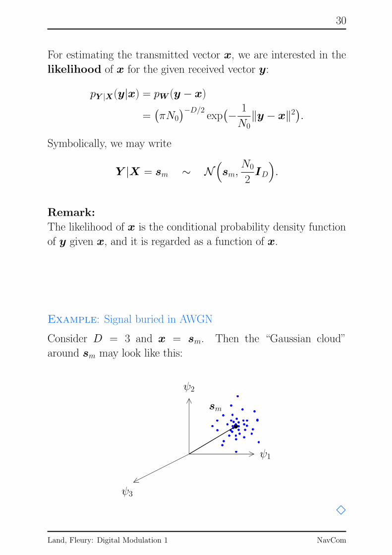
For estimating the transmitted vector x, we are interested in the
likelihood of x for the given received vector y:
pY |X(y|x) = pW (y − x)
=(πN0
)−D/2exp(− 1
N0‖y − x‖2
).
Symbolically, we may write
Y |X = sm ∼ N(
sm,N0
2ID
)
.
Remark:
The likelihood of x is the conditional probability density function
of y given x, and it is regarded as a function of x.
Example: Signal buried in AWGN
Consider D = 3 and x = sm. Then the “Gaussian cloud”
around sm may look like this:
PSfrag replacements
ψ1
ψ2
ψ3
sm
3
Land, Fleury: Digital Modulation 1 NavCom

31
1.8 Signal-to-Noise Ratio for the AWGNChannel
Consider a digital communication system using the set of wave-
forms
S ={
s1(t), s2(t), . . . , sM(t)}
,
sm(t) = 0 for t /∈ [0, T ], m = 1, 2, . . . ,M , for transmission over
an AWGN channel with power spectrum
SW (f ) =N0
2.
Let Esm denote the energy of waveform sm(t), and let Es denote
the average waveform energy:
Esm =
T∫
0
(sm(t)
)2dt, Es =
1
M
M∑
m=1
Esm
Thus, Es is the average energy per waveform x(t) and also
the average energy per vector x (due to the one-to-one correspon-
dence.)
The average signal-to-noise ratio (SNR) per waveform is
then defined as
γs =Es
N0.
Land, Fleury: Digital Modulation 1 NavCom

32
On the other hand, the average energy per source bit uk is of
interest. Since K source bits uk are transmitted per waveform, the
average energy per bit is
Eb =1
KEs.
Accordingly, the average signal-to-noise ratio (SNR) per
bit is then defined as
γb =Eb
N0.
As K bits are transmitted per waveform, we have the relation
γb =1
Kγs.
Remark:
The energies and signal-to-noise ratios usually denote received val-
ues.
Land, Fleury: Digital Modulation 1 NavCom

33
2 Optimum Decoding for theAWGN Channel
2.1 Optimality Criterion
In the previous chapter, the vector representation of a digital
transceiver transmitting over an AWGN channel was derived.
PSfrag replacements
BSS
BinarySink Vector
Vector
VectorEncoder
Decoder
AWGN
Channel
U
U
X
Y
W
Nomenclature
u = [u1, . . . , uK ] ∈ U, x = [x1, . . . , xD] ∈ X,
u = [u1, . . . , uK ] ∈ U, y = [y1, . . . , yD] ∈ RD,
U = {0, 1}K, X = {s1, . . . , sM}.
U : set of all binary sequences of length K,
X : set of vector representations of the waveforms.
The set X is called the signal constellation, and its elements
are called signals, signal points, or modulation symbols.
For convenience, we may refer to uk as bits and to x as symbols.
(But we have to be careful not to cause ambiguity.)
Land, Fleury: Digital Modulation 1 NavCom

34
As the vector representation implies no loss of information, re-
covering the transmitted block u = [u1, . . . , uK ] from the re-
ceived waveform y(t) is equivalent to recovering u from the vec-
tor y = [y1, . . . , yD].
Functionality of the vector encoder
enc : u 7→ x = enc(u)
U → X
Functionality of the vector decoder
decu : y 7→ u = decu(y)
RD → U
Optimality criterion
A vector decoder is called an optimal vector decoder if it
minimizes the block error probability Pr(U 6= U ).
2.2 Decision Rules
Since the encoder mapping is one-to-one, the functionality of the
vector decoder can be decomposed into the following two opera-
tions:
(i) Modulation-symbol decision:
dec : y 7→ x = dec(y)
RD → X
(ii) Encoder inverse:
enc−1 : x 7→ u = enc−1(x)
X → U
Land, Fleury: Digital Modulation 1 NavCom

35
Thus, we have the following chain of mappings:
ydec7→ x
enc−1
7→ u.
Block Diagram
PSfrag replacements
Vector
Encoder
Encoder
Vector Decoder
InverseMod. Symbol
Decision
enc
enc−1 dec
U
U
X
X Y
W
U
U X
X RD
RD
A decision rule is a function which maps each observation y ∈RD to a modulation symbol x ∈ X, i.e., to an element of the signal
constellation X.
Example: Decision rule
PSfrag replacements
RD
y(1)
y(2)
y(3)
{ },,, . . .s1 s2 sM = X
3
Land, Fleury: Digital Modulation 1 NavCom
36
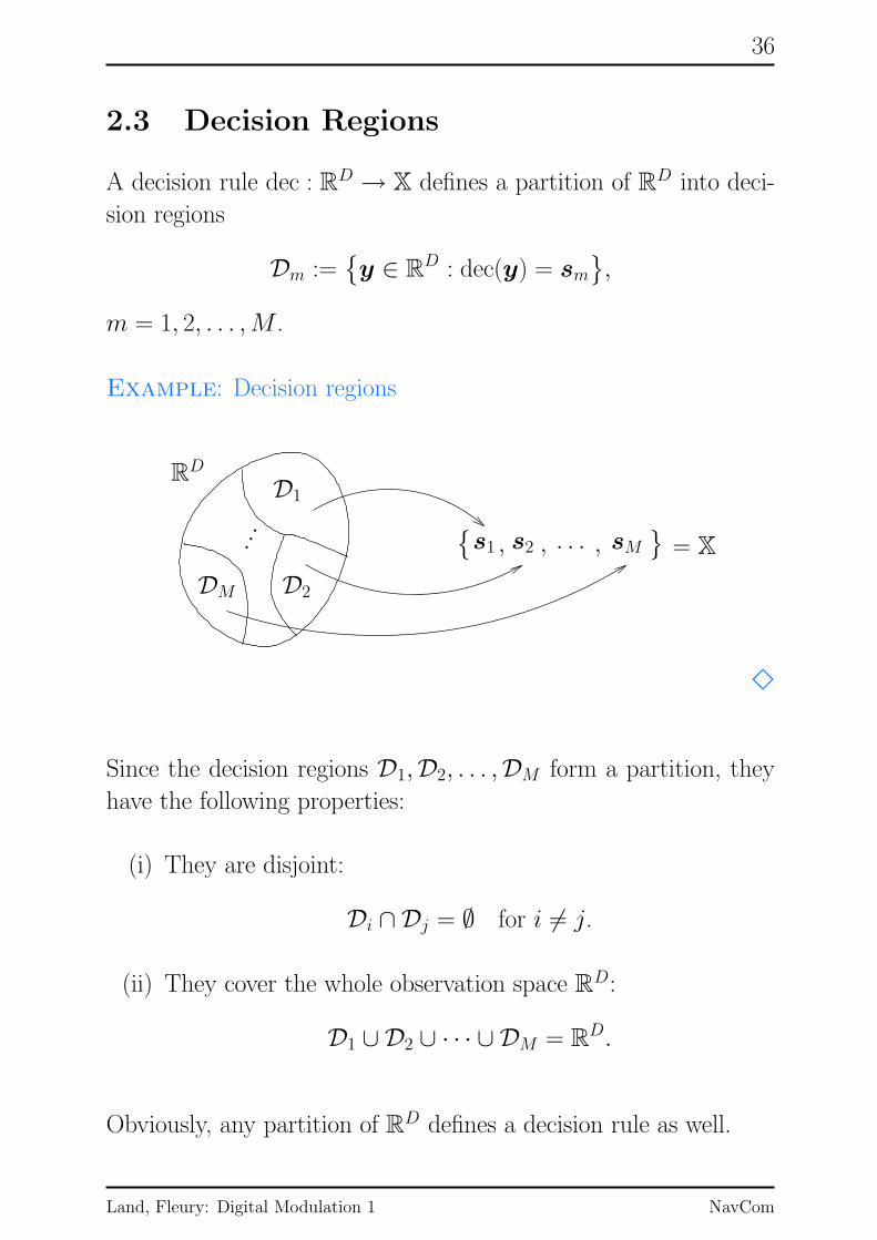
2.3 Decision Regions
A decision rule dec : RD → X defines a partition of R
D into deci-
sion regions
Dm :={y ∈ R
D : dec(y) = sm},
m = 1, 2, . . . ,M .
Example: Decision regions
...
PSfrag replacements
RD
D1
D2DM
{ },,, . . .s1 s2 sM = X
3
Since the decision regions D1,D2, . . . ,DM form a partition, they
have the following properties:
(i) They are disjoint:
Di ∩ Dj = ∅ for i 6= j.
(ii) They cover the whole observation space RD:
D1 ∪ D2 ∪ · · · ∪ DM = RD.
Obviously, any partition of RD defines a decision rule as well.
Land, Fleury: Digital Modulation 1 NavCom

37
2.4 Optimum Decision Rules
Optimality criterion for decision rules
Since the mapping enc : U → X of the vector encoder is one-to-
one, we have
U 6= U ⇔ X 6= X.
Therefore, the decision rule of an optimal vector decoder minimizes
the modulation-symbol error probability Pr(X 6= X).
Such a decision rule is called optimal.
Sufficient condition for an optimal decision rule
Let dec : RD → X be a decision rule which minimizes the
a-posteriori probability of making a decision error,
Pr(dec(y)︸ ︷︷ ︸
x
6= X∣∣Y = y
),
for any observation y. Then dec is optimal.
Remark:
The a-posteriori probability of a decoding error is
the probability of the event {dec(y) 6= X} conditioned on the
event {Y = y}:PSfrag replacements
Mod. SymbolDecision
dec
XX = dec(y) Y = y
W
Land, Fleury: Digital Modulation 1 NavCom

38
Proof:
Let dec : RD → X denote any decision rule, and let
decopt : RD → X denote an optimal decision rule. Then we
have
Pr(dec(Y ) 6= X
)=
∫
RD
Pr(dec(Y ) 6= X
∣∣Y = y
)· pY (y)dy
=
∫
RD
Pr(dec(y) 6= X
∣∣Y = y
)· pY (y)dy
(?)
≥∫
RD
Pr(decopt(y) 6= X
∣∣Y = y
)· pY (y)dy
=
∫
RD
Pr(decopt(Y ) 6= X
∣∣Y = y
)· pY (y)dy
= Pr(decopt(Y ) 6= X
).
(?): by definition of decopt, we have
Pr(dec(y) 6= X
∣∣Y = y
)≥ Pr
(decopt(y) 6= X
∣∣Y = y
)
for all x ∈ X.
Land, Fleury: Digital Modulation 1 NavCom

39
2.5 MAP Symbol Decision Rule
Starting with the necessary condition for an optimal decision rule
given above, we derive now a method to make an optimal decision.
The corresponding decision rule is called the maximum a-posteriori
(MAP) decision rule.
Consider an optimal decision rule
dec : y 7→ x = dec(y),
where the estimated modulation-symbol is denoted by x.
As the decision rule is assumed to be optimum, the probability
Pr(x 6= X|Y = y)
is minimal.
For any x ∈ X, we have
Pr(X 6= x|Y = y) = 1− Pr(X = x|Y = y)
= 1− pX|Y (x|y)
= 1− pY |X(y|x) pX(x)
pY (y),
where Bayes’ rule has been used in the last line. Notice that
Pr(X = x|Y = y) = pX|Y (x|y)
is the a-posteriori probability of {X = x} given {Y = y}.
Land, Fleury: Digital Modulation 1 NavCom
40
Using the above equalities, we can conclude that
Pr(X 6= x|Y = y) is minimal
⇔ pX|Y (x|y) is maximal
⇔ pY |X(y|x) pX(x) is maximal,
since pY (y) does not depend on x.
Thus, the estimated modulation-symbol x = dec(y) resulting from
the optimal decision rule satisfies the two equivalent conditions
pX|Y (x|y) ≥ pX|Y (x|y) for all x ∈ X;
pY |X(y|x) pX(x) ≥ pY |X(y|x) pX(x) for all x ∈ X.
These two conditions may be used to define the optimal decision
rule.
Maximum a-posteriori (MAP) decision rule:
x = decMAP(y) := argmaxx∈X
{
pX|Y (x|y)}
:= argmaxx∈X
{
pY |X(y|x) pX(x)}
.
The decision rule is called the MAP decision rule as the selected
modulation-symbol x maximizes the a-posteriori probability den-
sity function pX|Y (x|y). Notice that the two formulations are
equivalent.
Land, Fleury: Digital Modulation 1 NavCom
41
2.6 ML Symbol Decision Rule
If the modulation-symbols at the output of the vector encoder are
equiprobable, i.e., if
Pr(X = sm) =1
M
for m = 1, 2, . . . ,M , the MAP decision rule reduces to the follow-
ing decision rule.
Maximum likelihood (ML) decision rule:
x = decML(y) := argmaxx∈X
{
pY |X(y|x)}
.
In this case, the the selected modulation-symbol x maximizes the
likelihood function pY |X(y|x) of x.
Land, Fleury: Digital Modulation 1 NavCom

42
2.7 ML Decision for the AWGN Channel
Using the canonical decomposition of the transmitter and of the
receiver, we obtain the AWGN vector-channel:PSfrag replacements
X ∈ X Y ∈ RD
W ∼ N(
0, N02 ID
)
The conditional probability density function of Y given
X = x ∈ X is
pY |X(y|x) =(πN0
)−D/2exp(− 1
N0‖y − x‖2
).
Since exp(.) is a monotonically increasing function, we obtain the
following formulation of the ML decision rule
x = decML(y) = argmaxx∈X
{
pY |X(y|x)}
= argmaxx∈X
{
exp(− 1
N0‖y − x‖2
)}
= argminx∈X
{
‖y − x‖2}
.
Thus, the ML decision rule for the AWGN vector channel selects
the vector in the signal constellation X that is the closest one to the
observation y, where the distance measure is the squared Euclidean
distance.
Land, Fleury: Digital Modulation 1 NavCom

43
Implementation of the ML decision rule
The squared Euclidean distance can be expanded as
‖y − x‖2 = ‖y‖2 − 2〈y,x〉 + ‖x‖2.
The term ‖y‖2 is irrelevant for the minimization with respect to x.
Thus we get the following equivalent formulation of the ML decision
rule:
x = decML(y) = argminx∈X
{
−2〈y,x〉 + ‖x‖2}
= argmaxx∈X
{
2〈y,x〉 − ‖x‖2}
= argmaxx∈X
{
〈y,x〉 − 12‖x‖2
}
.
Block diagram of the ML decision rule for the AWGN vector-
channel:
......
PSfrag replacements
y s1
sM
12‖s1‖2
12‖sM‖2
x
selectlargest
one
Vector correlator:PSfrag replacements
a ∈ RD
b ∈ RD
〈a, b〉 =∑D
d=1 adbd ∈ R
Land, Fleury: Digital Modulation 1 NavCom

44
Remark:
Some signal constellations X have the property that ‖x‖2 has the
same value for all x ∈ X. In these cases (but only then), the ML
decision rule simplifies further to
x = decML(y) = argmaxx∈X
{
〈y,x〉}
.
2.8 Symbol-Error Probability
The error probability for modulation-symbols X , or for short, the
symbol-error probability is defined as
Ps = Pr(X 6= X) = Pr(dec(Y ) 6= X).
The symbol-error probability coincides with the block error prob-
ability
Ps = Pr(U 6= U ) = Pr(
[U1, . . . , UK ] 6= [U1, . . . , UK ])
.
We compute Ps in two steps:
(i) Compute the conditional symbol-error probability given
X = x for any x ∈ X:
Pr(X 6= X|X = x).
(ii) Average over the signal constellation:
Pr(X 6= X) =∑
x∈X
Pr(X 6= X|X = x) · Pr(X = x).
Land, Fleury: Digital Modulation 1 NavCom
45
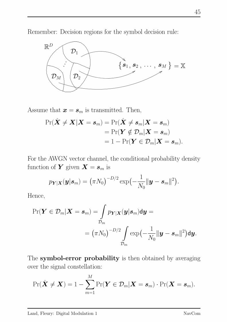
Remember: Decision regions for the symbol decision rule:
...
PSfrag replacements
RD
D1
D2DM
{ },,, . . .s1 s2 sM = X
Assume that x = sm is transmitted. Then,
Pr(X 6= X|X = sm) = Pr(X 6= sm|X = sm)
= Pr(Y /∈ Dm|X = sm)
= 1− Pr(Y ∈ Dm|X = sm).
For the AWGN vector channel, the conditional probability density
function of Y given X = sm is
pY |X(y|sm) =(πN0
)−D/2exp(− 1
N0‖y − sm‖2
).
Hence,
Pr(Y ∈ Dm|X = sm) =
∫
Dm
pY |X(y|sm)dy =
=(πN0
)−D/2∫
Dm
exp(− 1
N0‖y − sm‖2
)dy.
The symbol-error probability is then obtained by averaging
over the signal constellation:
Pr(X 6= X) = 1−M∑
m=1
Pr(Y ∈ Dm|X = sm) · Pr(X = sm).
Land, Fleury: Digital Modulation 1 NavCom
46
If the modulation symbols are equiprobable, the formula simplifies
to
Pr(X 6= X) = 1− 1
M
M∑
m=1
Pr(Y ∈ Dm|X = sm).
2.9 Bit-Error Probability
The error probability for the source bits Uk, or for short, the bit-
error probability is defined as
Pb =1
K
K∑
k=1
Pr(Uk 6= Uk),
i.e., as the average number of erroneous bits in the block
U = [U1, . . . , UK ].
Relation between the bit-error probability and the
symbol-error probability
Clearly, the relation between Pb and Ps depends on the encoding
function
enc : u = [u1, . . . , uk] 7→ x = enc(u).
The analytical derivation of the relation between Pb and Ps is
usually cumbersome. However, we can derive an upper bound
and a lower bound for Pb when Ps is given (and also vice versa).
These bounds are valid for any encoding function.
The lower bound provides a guideline for the design of a “good”
encoding function.
Land, Fleury: Digital Modulation 1 NavCom

47
Lower bound:
If a symbol is erroneous, there is at least one erroneous bit in the
block of K bits. Therefore
Pb ≥ 1KPs.
Upper bound:
If a symbol is erroneous, there are at most K erroneous bits in the
block of K bits. Therefore
Pb ≤ Ps.
Combination:
Combining the lower bound and the upper bound yields
1KPs ≤ Pb ≤ Ps.
An efficient encoder should achieve the lower bound for the bit-
error probability, i.e.,
Pb ≈ 1KPs.
Remark:
The bounds can also be obtained by considering the union bound
of the events
{U1 6= U1}, {U2 6= U2}, . . . , {UK 6= UK},i.e, by relating the probability
Pr(
{U1 6= U1} ∪ {U2 6= U2} ∪ . . . ∪ {UK 6= UK})
to the probabilities
Pr({U1 6= U1}
),Pr({U2 6= U2}
), . . . ,Pr
({UK 6= UK}
).
Land, Fleury: Digital Modulation 1 NavCom

48
2.10 Gray Encoding
In Gray encoding, blocks of bits, u = [u1, . . . , uK ], which differ in
only one bit uk are assigned to neighboring vectors (modulation
symbols) x in the signal constellation X.
Example: 4PAM (Pulse Amplitude Modulation)
Signal constellation: X = {[−3], [−1], [+1], [+3]}.
PSfrag replacements
00 01 1011
s1 s2 s3 s42−2
3
Motivation
When a decision error occurs, it is very likely that the transmitted
symbol and the detected symbol are neighbors. When the bit
blocks of neighboring symbols differ only in one bit, there will be
only one bit error per symbol error.
Effect
Gray encoding achieves
Pb ≈ 1KPs
for high signal-to-noise ratios (SNR).
Land, Fleury: Digital Modulation 1 NavCom

49
Sketch of the proof:
We consider the case K = 2, i.e., U = [U1, U2].
Ps = Pr(X 6= X)
= Pr(
[U1, U2] 6= [U1, U2])
= Pr(
{U1 6= U1} ∪ {U2 6= U2})
= Pr(U1 6= U1) + Pr(U2 6= U2)︸ ︷︷ ︸
2 · Pb− Pr
(
{U1 6= U1} ∩ {U2 6= U2})
︸ ︷︷ ︸
(?)
.
The term (?) is small compared to the other two terms if the SNR
is high. Hence
Ps ≈ 2 · Pb.
Land, Fleury: Digital Modulation 1 NavCom

50
Part II
Digital CommunicationTechniques
Land, Fleury: Digital Modulation 1 NavCom

51
3 Pulse Amplitude Modulation(PAM)
In pulse amplitude modulation (PAM), the information is conveyed
by the amplitude of the transmitted waveforms.
3.1 BPAM
PAM with only two waveforms is called binary PAM (BPAM).
3.1.1 Signaling Waveforms
Set of two rectangular waveforms with amplitudes A and −A over
t ∈ [0, T ], S :={s1(t), s2(t)
}:
PSfrag replacements
00TT
−A−A
AA
tt
s1(t) s2(t)
As |S| = 2, one bit is sufficient to address the waveforms (K = 1).
Thus, the BPAM transmitter performs the mapping
U 7→ x(t)
with
U ∈ U = {0, 1} and x(t) ∈ S.
Remark: In the general case, the basic waveform may also have
another shape.
Land, Fleury: Digital Modulation 1 NavCom

52
3.1.2 Decomposition of the Transmitter
Gram-Schmidt procedure
ψ1(t) =1√E1
s1(t)
with
E1 =
T∫
0
(s1(t)
)2dt =
T∫
0
A2dt = A2 · T.
Thus
ψ1(t) =
{1√T
for t ∈ [0, T ] ,
0 otherwise.
Both s1(t) and s2(t) are a linear combination of ψ(t):
s1(t) = +√
Es ψ1(t) = +A√T ψ1(t),
s2(t) = −√
Es ψ1(t) = −A√T ψ1(t),
where√Es = A
√T and Es = E1 = E2. (The two waveforms
have the same energy.)
Signal constellation
Vector representation of the two waveforms:
s1(t) ↔ s1 = s1 = +√
Es
s2(t) ↔ s2 = s2 = −√
Es
Thus the signal constellation is X ={−√Es,+
√Es
}.
PSfrag replacements
0
√Es
√Es
ψ1
s1s2
Land, Fleury: Digital Modulation 1 NavCom

53
Vector Encoder
The vector encoder is usually defined as
x = enc(u) =
{
+√Es for u = 0,
−√Es for u = 1.
The signal constellation comprises only two waveforms, and thus
per symbol and per bit, the average transmit energies and the
SNRs are the same:
Eb = Es, γs = γb.
3.1.3 ML Decoding
ML symbol decision rule
decML(y) = argminx∈{−√Es,+
√Es}‖y − x‖2 =
{
+√Es for y ≥ 0,
−√Es for y < 0.
Decision regions
D2 = {y ∈ R : y < 0}, D1 = {y ∈ R : y ≥ 0}.
PSfrag replacements
0
ψ1
y
s1 = +√Ess2 = −√Es
D1D2
Remark: The decision rule
decML(y) =
{
+√Es for y > 0,
−√Es for y ≤ 0.
is also a ML decision rule.
Land, Fleury: Digital Modulation 1 NavCom

54
The mapping of the encoder inverse reads
u = enc-1(x) =
{
0 for x = +√Es,
1 for x = −√Es.
Combining the (modulation) symbol decision rule and the encoder
inverse yields the ML decoder for BPAM:
u =
{
0 for y ≥ 0,
1 for y < 0.
3.1.4 Vector Representation of the Transceiver
BPAM transceiver:
PSfrag replacements
Encoder
Decoder
BSS
Sink
ψ1(t)
1√T
∫ T
0 (.)dt
U
U
X(t)X
Y (t)Y
W (t)0 7→ +
√Es
1 7→ −√Es
D1 7→ 0D2 7→ 1
Vector representation:
PSfrag replacements
Encoder
Decoder
BSS
Sink
1√T
∫ T
0 (.)dt
U
U
X
Y
W ∼ N (0, N0/2)
0 7→ +√Es
1 7→ −√Es
D1 7→ 0D2 7→ 1
Land, Fleury: Digital Modulation 1 NavCom

55
3.1.5 Symbol-Error Probability
Conditional probability densities
pY |X(y| +√
Es) =1√πN0
exp(− 1
N0|y −
√
Es|2)
pY |X(y| −√
Es) =1√πN0
exp(− 1
N0|y +
√
Es|2)
Conditional symbol-error probability
Assume that X = x = +√Es is transmitted.
Pr(X 6= X|X = +√
Es) = Pr(Y ∈ D2|X = +√
Es)
= Pr(Y < 0|X = +√
Es)
=1√πN0
0∫
−∞
exp(− 1
N0|y −
√
Es|2)dy
=1√2π
−√
2Es/N0∫
−∞
exp(−1
2z2)dz,
where the last equality results from substituting
z = (y −√
Es)/√
N0/2.
The Q-function is defined as
Q(v) :=
∞∫
v
q(z)dz, q(z) =1√2π
exp(−1
2z2).
Land, Fleury: Digital Modulation 1 NavCom

56
The function q(z) denotes a Gaussian pdf with zero mean and vari-
ance 1; i.e., it may be interpreted as the pdf of a random variable
Z ∼ N (0, 1).
Using this definition, the conditional symbol-error probabilities
may be written as
Pr(X 6= X|X = +√
Es) = Q(√
2Es
N0
)
,
Pr(X 6= X|X = −√
Es) = Q(√
2Es
N0
)
.
The second equation follows from symmetry.
Symbol-error probability
The symbol-error probability results from averaging over the con-
ditional symbol-error probabilities:
Ps = Pr(X 6= X)
= Pr(X = +√
Es) · Pr(X 6= X|X = +√
Es)
+ Pr(X = −√
Es) · Pr(X 6= X|X = −√
Es)
= Q(√
2Es
N0
)
= Q(√
2γs)
as Pr(X = +√Es) = Pr(X = −√Es) = 1/2.
Alternative method to derive the conditional symbol-
error probability
Assume again that X =√Es is transmitted. Instead of consider-
ing the conditional pdf of Y , we directly use the pdf of the white
Gaussian noise W .
Land, Fleury: Digital Modulation 1 NavCom

57
Pr(X 6= X|X = +√
Es) = Pr(Y < 0|X = +√
Es)
= Pr(√
Es +W < 0|X = +√
Es)
= Pr(W < −√
Es|X = +√
Es)
= Pr(W < −√
Es)
= Pr(W ′ < −√
2Es/N0)
= Q(√
2Es/N0),
where we substituted W ′ = W/√
N0/2; notice that
W ′ ∼ N (0, 1). A plot of the symbol-error probability can found
in [1, p. 412].
The initial event (here {Y < 0}) is transformed into an equivalent
event (here {W ′ < −√
2Es/N0}), of which the probability can
easily be calculated. This method is frequently applied to deter-
mine symbol-error probabilities.
3.1.6 Bit-Error Probability
In BPAM, each waveform conveys one source bit. Accordingly,
each symbol-error leads to exactly one bit-error, and thus
Pb = Pr(U 6= U) = Pr(X 6= X) = Ps.
Due to the same reason, the transmit energy per symbol is equal
to the transmit energy per bit, and so also the SNR per symbol is
equal to the SNR per bit:
Eb = Es, γs = γb.
Therefore, the bit-error probability (BEP) of BPAM results as
Pb = Q(√
2γb).
Notice: Pb ≈ 10−5 is achieved for γb ≈ 9.6 dB.
Land, Fleury: Digital Modulation 1 NavCom
58
3.2 MPAM
In the general case ofM -ary pulse amplitude modulation (MPAM)
with M = 2K , input blocks of K bits modulate the amplitude of
a unique pulse.
3.2.1 Signaling Waveforms
Waveform encoder:
u = [u1, . . . , uK ] 7→ x(t)
U = {0, 1}K → S ={s1(t), . . . , sM(t)
},
where
sm(t) =
{
(2m−M − 1)Ag(t) for t ∈ [0, T ],
0 otherwise,
A ∈ R, and g(t) is a predefined pulse of duration T ,
g(t) = 0 for t /∈ [0, T ].
Values of the factors (2m−M − 1)A that are weighting g(t):
−(M − 1)A,−(M − 3)A, . . . ,−A,A, . . . , (M − 3)A, (M − 1)A.
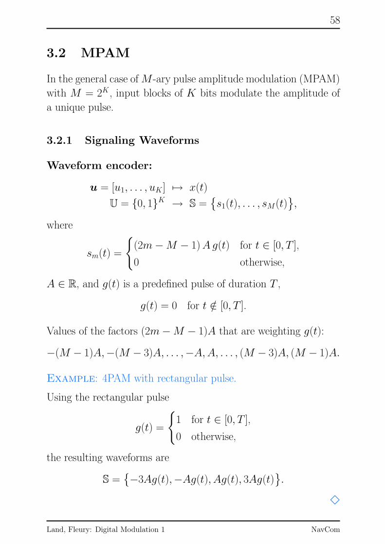
Example: 4PAM with rectangular pulse.
Using the rectangular pulse
g(t) =
{
1 for t ∈ [0, T ],
0 otherwise,
the resulting waveforms are
S ={−3Ag(t),−Ag(t), Ag(t), 3Ag(t)
}.
3
Land, Fleury: Digital Modulation 1 NavCom

59
3.2.2 Decomposition of the Transmitter
Gram-Schmidt procedure:
Orthonormal function
ψ(t) =1√E1
s1(t) =1
√Eg
g(t),
E1 =∫ T
0
(s1(t)
)2dt, Eg =
∫ T
0
(g(t))2
dt.
Every waveform in S is a linear combination of (only) ψ(t):
sm(t) = (2m−M − 1)A√
Eg︸ ︷︷ ︸
d
ψ(t)
= (2m−M − 1)d ψ(t).
Signal constellation
s1(t) ←→ s1 = −(M − 1)d
s2(t) ←→ s2 = −(M − 3)d
· · ·sm(t) ←→ sm = (2m−M − 1)d
· · ·sM−1(t) ←→ sM−1 = (M − 3)d
sM(t) ←→ sM = (M − 1)d
X ={s1, s2, . . . , sM
}
={−(M − 1)d,−(M − 3)d, . . . ,−d, d, . . .. . . , (M − 3)d, (M − 1)d
}.
Land, Fleury: Digital Modulation 1 NavCom

60
Example: M = 2, 4, 8
PSfrag replacements
0 1
00 01 1011
000 001 010011 100101110 111
s1
s1
s1
s2
s2
s2
s3
s3
s4
s4 s5 s6 s7 s8
3
Vector Encoder
The vector encoder
enc : u = [u1, . . . , uK ] 7→ x = enc(u)
U = {0, 1}K → X ={−(M − 1)d, . . . , (M − 1)d
}
is any Gray encoding function.
Energy and SNR
The source bits are generated by a BSS, and so the symbols of the
signal constellation X are equiprobable:
Pr(X = sm) =1
M
for all m = 1, 2, . . . ,M .
Land, Fleury: Digital Modulation 1 NavCom

61
The average symbol energy results as
Es = E[X2]
=1
M
M∑
m=1
(sm)2
=d2
M
M∑
m=1
(2m−M − 1)2 =d2
M
1
3M(M 2 − 1)
Thus,
Es =M 2 − 1
3d2 ⇐⇒ d =
√
3Es
M 2 − 1
As M = 2K , the average energy per transmitted source bit results
as
Eb =Es
K=M 2 − 1
3 log2Md2 ⇐⇒ d =
√
3 log2M
M 2 − 1Eb.
The SNR per symbol and the SNR per bit are related as
γb =1
Kγs =
1
log2Mγs.
Land, Fleury: Digital Modulation 1 NavCom

62
3.2.3 ML Decoding
ML symbol decision rule
decML(y) = argminx∈X
‖y − x‖2
Decision regions
Example: Decision regions for M = 4.
PSfrag replacements
D1 D2 D3 D4
s1 s2 s3 s4
0 2d−2d
y
3
Starting from the special cases M = 2, 4, 8, the decision regions
can be inferred:
D1 = {y ∈ R : y ≤ −(M − 2)d},D2 = {y ∈ R : −(M − 2)d < y ≤ −(M − 4)d},· · ·
Dm = {y ∈ R : (2m−M − 2)d < y ≤ (2m−M)d},· · ·
DM−1 = {y ∈ R : (M − 4)d < y ≤ (M − 2)d},DM = {y ∈ R : (M − 2)d < y}.
Accordingly, the ML symbol decision rule may also be written as
decML(y) = sm for y ∈ Dm.
ML decoder for MPAM
u = enc-1(decML(y))
Land, Fleury: Digital Modulation 1 NavCom

63
3.2.4 Vector Representation of the Transceiver
BPAM transceiver:
PSfrag replacements
GrayEncoder
Decoder
BSS
Sink
ψ(t)
1√T
∫ T
0 (.)dt
U
U
X(t)X
Y (t)Y
W (t)um 7→ sm
Dm 7→ um
Vector representation:
PSfrag replacements
GrayEncoder
Decoder
BSS
Sink
1√T
∫ T
0 (.)dtU
U
X
Y
W ∼ N (0, N0/2)um 7→ sm
Dm 7→ um
Notice: um denotes the block of source bits corresponding to sm,
i.e.,
sm = enc(um), um = enc-1(sm).
Land, Fleury: Digital Modulation 1 NavCom

64
3.2.5 Symbol-Error Probability
Conditional symbol-error probability
Two cases must be considered:
1. The transmitted symbol is an edge symbol (a symbol at the
edge of the signal constellation):
X ∈ {s1, sM}.
2. The transmitted symbol is not an edge symbol:
X ∈ {s2, s3, . . . , sM−1}.
Case 1: X ∈ {s1, sM}Assume first X = s1. Then
Pr(X 6= X|X = s1) = Pr(Y /∈ D1|X = s1)
= Pr(Y > s1 + d|X = s1)
= Pr(W > d)
= Pr( W√
N0/2>
d√
N0/2
)
= Q( d√
N0/2
)
.
Notice that W/√
N0/2 ∼ N (0, 1).
By symmetry,
Pr(X 6= X|X = sM) = Q( d√
N0/2
)
.
Land, Fleury: Digital Modulation 1 NavCom

65
Case 2: X ∈ {s2, . . . , sM−1}Assume X = sm. Then
Pr(X 6= X|X = sm) = Pr(Y /∈ Dm|X = sm)
= Pr(W < −d or W > d)
= Pr(W < −d) + Pr(W > d)
= Pr( W√
N0/2< − d
√
N0/2
)
+ Pr( W√
N0/2>
d√
N0/2
)
= Q( d√
N0/2
)
+Q( d√
N0/2
)
= 2 ·Q( d√
N0/2
)
.
Symbol-error probability
Averaging over the symbols, one obtains
Ps =1
M
M∑
m=1
Pr(X 6= X|X = sm)
=2
MQ( d√
N0/2
)
+2(M − 2)
MQ( d√
N0/2
)
= 2M − 1
MQ( d√
N0/2
)
.
Expressing the symbol-error probability as a function of the SNR
per symbol, γs, or the SNR per bit, γb, yields
Ps = 2M − 1
MQ(√
6
M 2 − 1γs
)
= 2M − 1
MQ(√
6 log2M
M 2 − 1γb
)
.
Land, Fleury: Digital Modulation 1 NavCom

66
Plots of the symbol-error probabilities can be found in [1, p. 412].
Remark: When comparing BPAM and 4PAM for the same Ps,
the SNRs per bit, γb, differ by 10 log10(5/2) ≈ 4 dB. (Proof?)
3.2.6 Bit-Error Probability
When Gray encoding is used, we have the relation
Pb ≈Ps
log2M
= 2M − 1
M log2MQ(√
6 log2M
M 2 − 1γb
)
for high SNR γb = Eb/N0.
Land, Fleury: Digital Modulation 1 NavCom

67
4 Pulse Position Modulation (PPM)
In pulse position modulation (PPM), the information is conveyed
by the position of the transmitted waveforms.
4.1 BPPM
PPM with only two waveforms is called binary PPM (BPPM).
4.1.1 Signaling Waveforms
Set of two rectangular waveforms with amplitude A and dura-
tion T/2 over t ∈ [0, T ], S :={s1(t), s2(t)
}:
PSfrag replacements
00TT T
2T2 −A−A
AA
t t
s1(t) s2(t)
As the cardinality of the set is |S| = 2, one bit is sufficient to
address each waveforms, i.e., K = 1. Thus, the BPPM transmitter
performs the mapping
U 7→ x(t)
with
U ∈ U = {0, 1} and x(t) ∈ S.
Remark: In the general case, the basic waveform may also have
another shape.
Land, Fleury: Digital Modulation 1 NavCom

68
4.1.2 Decomposition of the Transmitter
Gram-Schmidt procedure
The waveforms s1(t) and s2(t) are orthogonal and have the same
energy
Es =
T∫
0
s21(t)dt =
T∫
0
s22(t)dt = A2 · T2 .
Notice that√Es = A
√
T/2.
The two orthonormal functions and the corresponding waveform
representations are
ψ1(t) =1√Es
s1(t), s1(t) =√
Es · ψ1(t) + 0 · ψ2(t),
ψ2(t) =1√Es
s2(t), s2(t) = 0 · ψ1(t) +√
Es · ψ2(t).
Signal constellation
Vector representation of the two waveforms:
s1(t) ←→ s1 = (√
Es, 0)T,
s2(t) ←→ s2 = (0,√
Es)T.
Thus the signal constellation is X ={(√Es, 0)T, (0,
√Es)
T}.
PSfrag replacements
00
√Es
√Es
√2Es
ψ1
ψ2
s1
s2
Land, Fleury: Digital Modulation 1 NavCom

69
Vector Encoder
The vector encoder is defined as
x = enc(u) =
{
(√Es, 0)T for u = 0,
(0,√Es)
T for u = 1.
The signal constellation comprises only two waveforms, and thus
per (modulation) symbol and per (source) bit, the average transmit
energies and the SNRs are the same:
Eb = Es, γs = γb.
4.1.3 ML Decoding
ML symbol decision rule
decML(y) = argminx∈{s1,s2}
‖y − x‖2 =
{
(√Es, 0)T for y1 ≥ y2,
(0,√Es)
T for y1 < y2.
Notice: ‖y − s1‖2 ≤ ‖y − s2‖2 ⇔ y1 ≥ y2.
Decision regions
D1 = {y ∈ R2 : y1 ≥ y2}, D2 = {y ∈ R
2 : y1 < y2}.PSfrag replacements
00
√Es
√Es
√2Es
y1
y2
s1
s2 D1
D2
Land, Fleury: Digital Modulation 1 NavCom

70
Combining the (modulation) symbol decision rule and the encoder
inverse yields the ML decoder for BPPM:
u = enc-1(decML(y)) =
{
0 for y1 ≥ y2,
1 for y1 < y2.
The ML decoder may be implemented by
PSfrag replacements
UY1
Y2
Z z ≥ 0→ 0
z < 0→ 1
Notice that Z = Y1 − Y2 is then the decision variable.
Land, Fleury: Digital Modulation 1 NavCom

71
4.1.4 Vector Representation of the Transceiver
BPPM transceiver for the waveform AWGN channel
PSfrag replacements
Vector
VectorEncoder
Decoder
BSS
Sink
0 7→ (√Es, 0)
T
1 7→ (0,√Es)
T
ψ1(t)
ψ2(t)
√2
T
∫ T/2
0(.)dt
√2
T
∫ T
T/2(.)dt
D1 7→ 0D2 7→ 1
U
U
X(t)X1
X2
Y (t)
Y1
Y2
W (t)
Vector representation including a AWGN vector channel
PSfrag replacements
Vector
VectorEncoder
Decoder
BSS
Sink
0 7→ (√Es, 0)
T
1 7→ (0,√Es)
T
ψ1(t)
ψ2(t)√2
T
∫ T/2
0(.)dt
√2T
∫ T
T/2(.)dt
D1 7→ 0D2 7→ 1
U
U
X1
X2
Y1
Y2
W1 ∼ N (0, N0/2)
W2 ∼ N (0, N0/2)
Land, Fleury: Digital Modulation 1 NavCom

72
4.1.5 Symbol-Error Probability
Conditional symbol-error probability
Assume that X = s1 = (√Es, 0)T is transmitted.
Pr(X 6= X|X = s1) = Pr(Y ∈ D2|X = s1)
= Pr(s1 + W ∈ D2|X = s1)
= Pr(s1 + W ∈ D2)
The noise vector W may be represented in the coordinate system
(ξ1, ξ2) or in the rotated coordinate system (ξ ′1, ξ′2). The latter is
more suited to computing the above probability, as only the noise
component along the ξ ′2-axis is relevant.
PSfrag replacements
0
√Es
√Es
√
Es/2
ξ1
ξ2
ξ′1
ξ′2
α = π/4
s1
s2 s1 + w
w1
w2
w′1
w′2
D1
D2
The elements of the noise vector in the rotated coordinate system
have the same statistical properties as in the non-rotated coordi-
nate system (see Appendix B), i.e.,
W ′1 ∼ N (0, N0/2), W ′
2 ∼ N (0, N0/2).
Land, Fleury: Digital Modulation 1 NavCom

73
Thus, we obtain
Pr(X 6= X|X = s1) = Pr(W ′2 >
√
Es/2)
= Pr(W ′
2√
N0/2>
√
Es
N0)
= Q(√
Es/N0) = Q(√γs).
By symmetry,
Pr(X 6= X|X = s2) = Q(√γs).
Symbol-error probability
Averaging over the conditional symbol-error probabilities, we ob-
tain
Ps = Pr(X 6= X) = Q(√γs).
4.1.6 Bit-Error Probability
For BPPM, Eb = Es, γs = γb, Pb = Ps (see above), and so the
bit-error probability (BEP) results as
Pb = Pr(U 6= U) = Q(√γb).
A plot of the BEP versus γb may be found in [1, p. 426]
Remark
Due to their signal constellations, BPPM is called orthogonal sig-
naling and BPAM is called antipodal signaling. Their BEPs are
given by
Pb,BPPM = Q(√γb), Pb,BPAM = Q(
√
2γb).
When comparing the SNR for a certain BEP, BPPM requires 3 dB
more than BPAM. For a plot, see [1, p. 409]
Land, Fleury: Digital Modulation 1 NavCom

74
4.2 MPPM
In the general case of M -ary pulse position modulation (MPPM)
with M = 2K , input blocks of K bits determine the position of a
unique pulse.
4.2.1 Signaling Waveforms
Waveform encoder
u = [u1, . . . , uK ] 7→ x(t)
U = {0, 1}K → S ={s1(t), . . . , sM(t)
},
where
sm(t) = g(
t− (m− 1)T
M
)
,
m = 1, 2, . . . ,M , and g(t) is a predefined pulse of duration T/M ,
g(t) = 0 for t /∈ [0, T/M ].
The waveforms are orthogonal and have the same energy as g(t),
Es = Eg =
T∫
0
g2(t)dt.
Example: (M=4)
Consider a rectangular pulse g(t) with amplitude A and du-
ration T/4. Then, we have the set of four waveforms, S =
{s1(t), s2(t), s3(t), s4(t)}:PSfrag replacements
00
T
A
t
s1(t)
PSfrag replacements
00
T
A
ts1(t)
s2(t)
PSfrag replacements
00
T
A
t
s1(t)
s2(t)
s3(t)
PSfrag replacements
00
T
A
t
s1(t)
s2(t)
s3(t)
s4(t)
3
Land, Fleury: Digital Modulation 1 NavCom

75
4.2.2 Decomposition of the Transmitter
Gram-Schmidt procedure
As all waveforms are orthogonal, we have M orthonormal func-
tions:
ψm(t) =1√Es
sm(t),
m = 1, 2, . . . ,M .
The waveforms and the orthonormal functions are related as
sm(t) =√
Es · ψm(t),
m = 1, 2, . . . ,M .
Signal constellation
Waveforms and their vector representations:
s1(t) ←→ s1 = (
M︷ ︸︸ ︷√
Es, 0, 0, . . . , 0)T
s2(t) ←→ s2 = (0,√
Es, 0, . . . , 0)T
...
sM(t) ←→ sM = (0, 0, 0, . . . ,√
Es)T
Signal constellation:
X ={s1, s2, . . . , sM
}∈ R
M .
The modulation symbols x ∈ X are orthogonal, and they are
placed on corners of an M -dimensional hypercube.
Land, Fleury: Digital Modulation 1 NavCom

76
Example: M = 3
The signal constellation
X ={(√
Es, 0, 0)T, (0,√
Es, 0)T, (0,√
Es, 0)T}∈ R
3
may be visualized using a cube with side-length√Es. 3
Vector Encoder
enc : u = [u1, . . . , uK ] 7→ x = enc(u)
U = {0, 1}K → X ={s1, s2, . . . , sM
}
Energy and SNR
The symbol energy is Es, and as M = 2K , the average energy per
transmitted source bit results as
Eb =Es
K
The SNR per symbol and the SNR per bit are related as
γb =1
Kγs =
1
log2Mγs.
Land, Fleury: Digital Modulation 1 NavCom
77
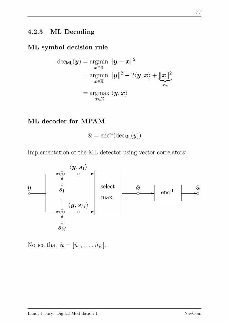
4.2.3 ML Decoding
ML symbol decision rule
decML(y) = argminx∈X
‖y − x‖2
= argminx∈X
‖y‖2 − 2〈y,x〉 + ‖x‖2︸︷︷︸Es
= argmaxx∈X
〈y,x〉
ML decoder for MPAM
u = enc-1(decML(y))
Implementation of the ML detector using vector correlators:
...
PSfrag replacements
enc-1y s1
sM
〈y, s1〉
〈y, sM〉
x uselect
max.
Notice that u = [u1, . . . , uK ].
Land, Fleury: Digital Modulation 1 NavCom

78
4.2.4 Symbol-Error Probability
Conditional symbol-error probability
Assume first that X = s1 is transmitted. Then
Pr(X 6= X|X = s1) = 1− Pr(X = X|X = s1)
= 1− Pr(
〈y, s1〉 ≥ 〈y, sm〉 for all m 6= 1|X = s1
)
.
For X = s1 = (√Es, 0, . . . , 0), the received vector is
Y = s1 + W = (√
Es, 0, . . . , 0) + (W1, . . . ,WM),
so that
〈y, sm〉 =
{
Es +√Es ·W1 for m = 1,√
Es ·Wm for m = 2, . . . ,M .
Therefore, the symbol-error probability may be written as follows:
Pr(X 6= X|X = s1) =
= 1− Pr(Es +
√
EsW1 ≥√
EsWm for all m 6= 1)
= 1− Pr(√
Es
N0/2+
W1√
N0/2︸ ︷︷ ︸
W ′1
≥ Wm√
N0/2︸ ︷︷ ︸
W ′m
for all m 6= 1)
= 1− Pr(W ′
m ≤√
2Es
N0+W ′
1 for all m 6= 1)
with
W ′ = (W ′1, . . . ,W
′M)T ∼ N (0, I),
i.e., the componentsW ′m are independent and Gaussian distributed
with zero mean and variance 1.
Land, Fleury: Digital Modulation 1 NavCom

79
The probability is now written using the pdf of W ′1:
Pr(W ′
m ≤√
2Es
N0+W ′
1 for all m 6= 1)
=
=
+∞∫
−∞
Pr(W ′
m ≤√
2Es
N0+W ′
1 for all m 6= 1∣∣W ′
1 = v)
︸ ︷︷ ︸
(?)
pW ′1(v)dv.
The events corresponding to different values of m are independent,
and thus
(?) =
M∏
m=2
Pr(W ′
m ≤√
2Es
N0+W ′
1
∣∣W ′
1 = v)
︸ ︷︷ ︸
Pr(W ′
m ≤√
2Es
N0+ v)
=
M∏
m=2
Q(√
2Es
N0+ v)
= QM−1(√
2γs + v).
Using this result and inserting pW ′1(v), we obtain the conditional
symbol-error probability
Pr(X 6= X|X = s1) =
=
+∞∫
−∞
[
1− QM−1(√
2γs + v)] 1√
2πexp(−v
2
2
)dv
Symbol-error probability
The above expression is independent of s1 and thus valid for all
x ∈ X. Therefore, the average symbol-error probability results as
Ps =
+∞∫
−∞
[
1− QM−1(√
2γs + v)] 1√
2πexp(−v
2
2
)dv.
Land, Fleury: Digital Modulation 1 NavCom
80
4.2.5 Bit-Error Probability
Hamming distance
The Hamming distance dH(u,u′) between two length-K vectors
u and u′ is the number of positions in which they differ:
dH(u,u′) =
K∑
k=1
δ(uk, u′k),
where the indicator function is defined as
δ(u, u′) =
{
1 for u = u′,
0 for u 6= u′.
Example: 4PPM
Let the blocks of source bits and the modulation symbols be asso-
ciated as
u1 = enc-1(s1) = [0, 0]
u2 = enc-1(s2) = [0, 1]
u3 = enc-1(s3) = [1, 0]
u4 = enc-1(s4) = [1, 1].
Then we have for example
dH(u1,u1) = 0, dH(u1,u2) = 1,
dH(u2,u3) = 2, dH(u2,u4) = 1.
3
Land, Fleury: Digital Modulation 1 NavCom
81
Conditional bit-error probability
Assume that X = s1, and let
um = [um,1, . . . , um,K ] = enc-1(sm).
The conditional bit-error probability is defined as
Pr(U 6= U |X = s1) =1
K
K∑
k=1
Pr(Uk 6= Uk|X = s1).
The argument of the sum may be expanded as
Pr(Uk 6= Uk|X = s1) =
=
M∑
m=1
Pr(Uk 6= Uk|X = sm,X = s1) Pr(X = sm|X = s1).
Since
X = s1 ⇔ U = u1 ⇒ Uk = u1,k,
X = sm ⇔ U = um ⇒ Uk = um,k,
we have
Pr(Uk 6= Uk|X = sm,X = s1) =
= Pr(u1,k 6= um,k|X = sm,X = s1)
= δ(u1,k, um,k).
Using this result in the expression for the conditional bit-error
probability, we obtain
Pr(U 6= U |X = s1)
=1
K
K∑
k=1
M∑
m=1
δ(u1,k, um,k) Pr(X = sm|X = s1)
=1
K
M∑
m=1
K∑
k=1
δ(u1,k, um,k)
︸ ︷︷ ︸
dH(u1,um)
Pr(X = sm|X = s1)
Land, Fleury: Digital Modulation 1 NavCom

82
Due to the symmetry of the signal constellation, the probabilities
of making a specific decision error are identical, i.e.,
Pr(X = sm|X = sm′) =Ps
M − 1=
Ps2K − 1
for all m 6= m′. Using this in the above sum yields
Pr(U 6= U |X = s1) =1
K· Ps2K − 1
M∑
m=1
dH(u1,um).
Without loss of generality, we assume u1 = 0. The sum over the
Hamming distances becomes then the overall number of ones in all
bit blocks of length K.
Example:
Consider K = 3 and write the binary vectors of length 3 in the
columns of a matrix:
[uT
1 , . . . ,uT8
]=
0 0 0 0 1 1 1 1
0 0 1 1 0 0 1 1
0 1 0 1 0 1 0 1
.
In every row, half of the entries are ones. The overall number of
ones is thus 3 · 23−1. 3
Generalizing the example, the above sum can shown to be
M∑
m=1
dH(0,um) = K · 2K−1.
Land, Fleury: Digital Modulation 1 NavCom
83
Applying this result, we obtain the conditional bit-error probability
Pr(U 6= U |X = s1) =2K−1
2K − 1· Ps,
which is independent of s1 and thus the same for all transmitted
symbols X = sm, m = 1, . . . ,M .
Average bit-error probability
From above, we obtain
Pr(U 6= U) =2K−1
2K − 1· Ps.
Plots of the BEPs may be found in [1, p. 426]
Notice that for large K,
Pr(U 6= U) ≈ 1
2· Ps.
Due to the signal constellation, Gray mapping is not possible.
Land, Fleury: Digital Modulation 1 NavCom

84
Remarks
(i) Provided that the SNR γb = Eb/N0 is larger than ln 2 (cor-
responding to −1.6 dB), the BEP of MPPM can be
made arbitrarily small by selecting M large enough.
The price to pay is an increasing decoding delay and an in-
creasing required bandwidth.
Let the transmission rate be denoted by
R =K
T=
log2M
T[bit/sec].
Decoding delay:
T =1
R· log2M.
Hence, for a fixed rate R, T →∞ for M →∞.
Required bandwidth:
B = Bg ≈1
T/M=M
T= R · M
log2M,
where Bg denotes the bandwidth of the pulse g(t).
Hence, for a fixed rate R, B →∞ for M →∞.
(ii) The power of the MPPM signal is
P =Eb ·KT
= Eb ·R.
Hence, the condition γb > ln 2 is equivalent to the condition
R <1
ln 2· PN0
= C∞.
The value C∞ denotes the capacity of the (infinite band-
width) AWGN channel (see Appendix C).
Land, Fleury: Digital Modulation 1 NavCom

85
5 Phase-Shift Keying (PSK)
In phase-shift keying (PSK), the waveforms are sines with the same
frequency, and the information is conveyed by the phase of the
waveforms.
5.1 Signaling Waveforms
Set of sines sm(t) with the same frequency f0, duration T , and
different phases φm:
sm(t) =
√2P cos
(2πf0t + 2πm−1
M︸ ︷︷ ︸
φm
)for t ∈ [0, T ],
0 elsewhere,
m = 1, 2, . . . ,M . The phase can take the values
φm ∈{0, 2π 1
M , 2π2M , . . . , 2π
M−1M
}
Hence, the digital information is embedded in the phase of a carrier.
The frequency f0 is called the carrier frequency.
For M = 2, this modulation scheme is called binary phase-
shift keying (BPSK), and for M = 4, it is called quadrature
phase-shift keying. (QPSK).
All waveforms have the same energy
Es =
∞∫
−∞
s2m(t)dt = PT.
(Notice: cos2 x = 1 + cos 2x.)
Land, Fleury: Digital Modulation 1 NavCom

86
Usually, f0 � 1/T . For simplifying the theoretical analysis, we
assume that f0 = L/T for some large L ∈ N.
BPSK
For M = 2, we obtain φm ∈ {0, π} and thus the two waveforms
s1(t) =√
2P cos(2πf0t
),
s2(t) =√
2P cos(2πf0t + π
)= −s1(t)
for t ∈ [0, T ].
QPSK
For M = 4, we obtain φm ∈ {0, π2 , π, 3π2 } and thus the waveforms
are
s1(t) = +√
2P cos(2πf0t
),
s2(t) = −√
2P sin(2πf0t
),
s3(t) = −√
2P cos(2πf0t
),
s4(t) = +√
2P sin(2πf0t
)
for t ∈ [0, T ].
Land, Fleury: Digital Modulation 1 NavCom

87
5.2 Signal Constellation
BPSK
Orthonormal functions:
ψ1(t) = 1√Ess1(t) =
√2T cos
(2πf0t
)
for t ∈ [0, T ].
Geometrical representation of the waveforms:
s1(t) = +√PTψ1(t) ←→ s1 = +
√PT = +
√
Es
s2(t) = −√PTψ1(t) ←→ s2 = −
√PT = −
√
Es
Signal constellation:
PSfrag replacements
0
√Es
√Es
ψ1
s1s2
Vector encoder:
x = enc(u) =
{
s1 for u = 1,
s2 for u = 0.
Land, Fleury: Digital Modulation 1 NavCom

88
QPSK
Orthonormal functions:
ψ1(t) = 1√Ess1(t) = +
√2T cos
(2πf0t
)
ψ2(t) = 1√Ess2(t) = −
√2T sin
(2πf0t
)
for t ∈ [0, T ].
Geometrical representation of the waveforms:
s1(t) = +√PTψ1(t) ←→ s1 = (
√
Es, 0)T
s2(t) =√
Esψ2(t) ←→ s2 = (0,√
Es)T
s3(t) = −√PTψ1(t) ←→ s3 = (−
√
Es, 0)T
s4(t) = −√
Esψ2(t) ←→ s4 = (0,−√
Es)T
with Es = PT .
Signal constellation:
PSfrag replacements
ψ1
ψ2
s1
s2
s3
s4
Vector encoder: any Gray encoder
Land, Fleury: Digital Modulation 1 NavCom
89
General Case
The expression for sm(t) can be expanded as follows:
sm(t) =√
Es cos(2πf0t + φm
)
=√
Es cosφm cos(2πf0t)−√
Es sinφm sin(2πf0t),
where φm = 2πm−1M , m = 1, 2, . . . ,M .
(Notice: cos(x + y) = cos x cos y − sinx sin y.)
Orthonormal functions:
ψ1(t) =√
2T cos(2πf0t)
ψ2(t) = −√
2T sin
(2πf0t
)
for t ∈ [0, T ].
Geometrical representation of the waveforms:
sm(t) =√
Es cosφm · ψ1(t) +√
Es sinφm · ψ2(t)
←→ sm =(√
Es cosφm,√
Es sinφm)T,
m = 1, 2, . . . ,M . Remember: Es = PT .
Signal constellation:
X ={(√
Es cos 2πm−1M ,
√
Es sin 2πm−1M
)T: m = 1, 2, . . . ,M
}
Example: 8PSK
For M = 8, we obtain φm = πm−14 , m = 1, 2, . . . , 8. (Figure?) 3
Land, Fleury: Digital Modulation 1 NavCom

90
5.3 ML Decoding
ML symbol decision rule
decML(y) = argminx∈X
‖y − x‖2
ML decoder for MPSK
u = [u1, u2, . . . , uK ] = enc-1(decML(y))
BPSK
BPSK has the same signal constellation as BPAM. Thus, the ML
detectors for these two modulation schemes are the same.
PSfrag replacements
0
ψ1
ys1
(u = 1)
s2
(u = 0)
D1D2
Implementation of the ML detector:PSfrag replacements
UY
y < 0→ 0
y ≥ 0→ 1
Land, Fleury: Digital Modulation 1 NavCom

91
QPSK
Decision regions for the symbols sm and corresponding bit blocks
u = [u1, u2] (Gray encoding):
PSfrag replacements
y1
y2
s1
s2
s3
s4
00
01
10
11
D1
D2
D3
D4
Decision rule for the data bits:
u1 =
{
0 for y ∈ D1 ∪ D2 ⇔ y1 + y2 > 0
1 for y ∈ D3 ∪ D4 ⇔ y1 + y2 < 0
u2 =
{
0 for y ∈ D1 ∪ D4 ⇔ y2 − y1 < 0
1 for y ∈ D2 ∪ D3 ⇔ y2 − y1 > 0
Implementation of the ML decoder:
PSfrag replacements
Y1
Y2
Z1
Z2
U1
U2
z1 > 0→ 0
z1 < 0→ 1
z2 < 0→ 0
z2 > 0→ 1
Land, Fleury: Digital Modulation 1 NavCom
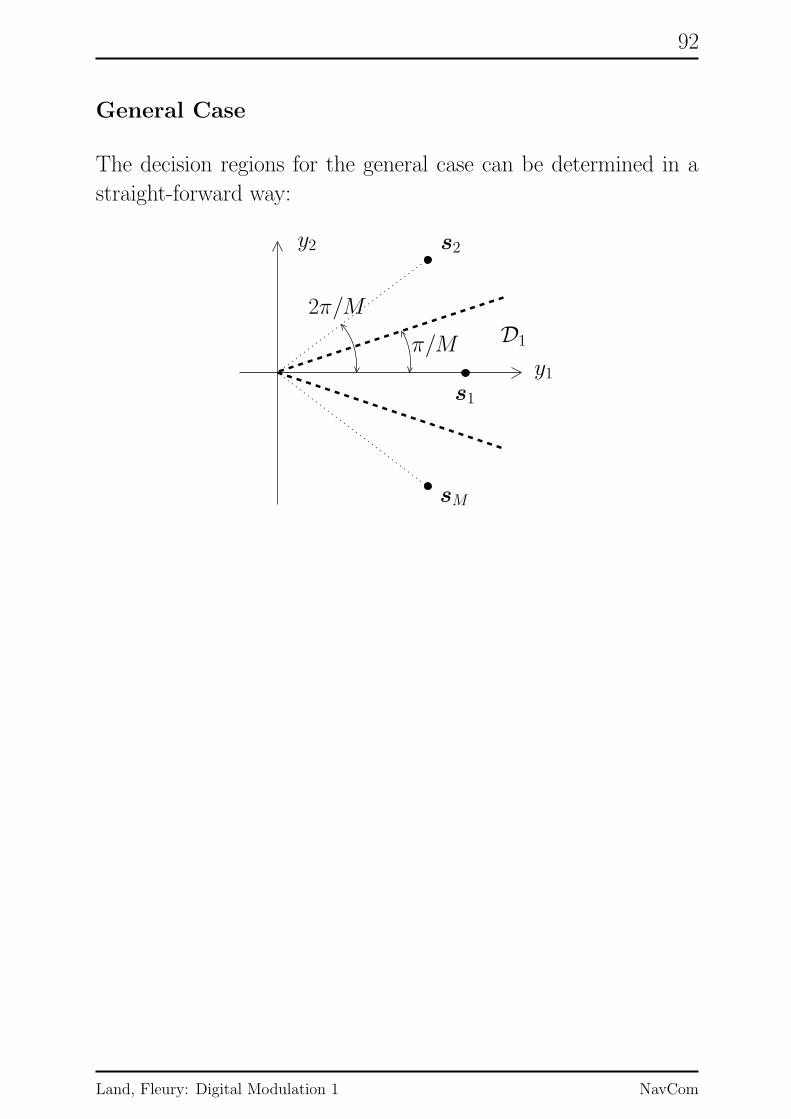
92
General Case
The decision regions for the general case can be determined in a
straight-forward way:
PSfrag replacements
y1
y2
s1
s2
sM
D1π/M
2π/M
Land, Fleury: Digital Modulation 1 NavCom

93
5.4 Vector Representation of the MPSKTransceiver
PSfrag replacements
Vector
Vector
Encoder
Decoder
AWGN Vector ChannelU X(t)
X1
X2
W (t)
Y (t)
Y1
Y2
U
T
T
√2
T
√2
T
cos 2πf0t
cos 2πf0t
− sin 2πf0t
− sin 2πf0t
√2
T
∫ T
0(.)dt
√2
T
∫ T
0(.)dt
AWGN Vector Channel:
PSfrag replacements
X1
X2
W1 ∼ N (0, N0/2)
W2 ∼ N (0, N0/2)
Y1
Y2
Land, Fleury: Digital Modulation 1 NavCom

94
5.5 Symbol-Error Probability
BPSK
Since BPSK has the same signal constellation as BPAM, the two
modulation schemes have the same symbol-error probability:
Ps = Q(√
2Es
N0
)
= Q(√
2γs).
QPSK
Assume that X = s1 is transmitted. Then, the conditional
symbol-error probability is given by
Pr(X 6= X|X = s1) = Pr(y /∈ D1|X = s1)
= 1− Pr(y ∈ D1|X = s1)
= 1− Pr(s1 + W ∈ D1).
For computing this probability, the noise vector is projected on the
rotated coordinate system (ξ ′1, ξ′2) (compare BPPM):
PSfrag replacements
0
√Es
√
Es/2
y1
y2
ξ1
ξ2
ξ′1
ξ′2
π/4
s1
s2
s1 + w
w1
w2
w′1
w′2
D1
D2
D3
D4
decis
ionbo
unda
ry
decisionboundary
Land, Fleury: Digital Modulation 1 NavCom

95
The probability may then be written as
Pr(s1 + W ∈ D1) = Pr(
W ′1 > −
√Es
2 and W ′2 <
√Es
2
)
= Pr(
W ′1 > −
√Es
2
)
· Pr(
W ′2 <
√Es
2
)
= Pr(
W ′1√N0/2
> −√
Es
N0
)
· Pr(
W ′2√N0/2
<√
Es
N0
)
=(
1− Q(√γs))(
1− Q(√γs))
=(
1− Q(√γs))2
.
Hence,
Pr(X 6= X|X = s1) = 1−(
1− Q(√γs))2
= 2 Q(√γs)− Q2(
√γs).
By symmetry, the four conditional symbol-error probabilities are
identical, and thus the average symbol-error probability results as
Ps = 2 Q(√γs)− Q2(
√γs).
Land, Fleury: Digital Modulation 1 NavCom

96
General Case
A closed-form expression for Ps does not exist. It can be upper-
bounded using an union-bound technique, or it can be numerically
computed using an integral expression. (See literature.) A plot of
Ps versus the SNR can be found in [1, p. 416].
Remark: Union Bound
For two random events A and B, we have
Pr(A ∪B) = Pr(A) + Pr(B)− Pr(A ∩B)︸ ︷︷ ︸
≤ 0
≤ Pr(A) + Pr(B).
The expression on the right-hand side is called the union bound for
the probability on the left-hand side. In a similar way, we obtain
the union bound for multiple events:
Pr(A1 ∪ A2 ∪ · · · ∪ AM) ≤ Pr(A1) + Pr(A2) + · · · + Pr(AM).
Each of these events may denote the case that the received vector
is within a certain decision region.
Land, Fleury: Digital Modulation 1 NavCom
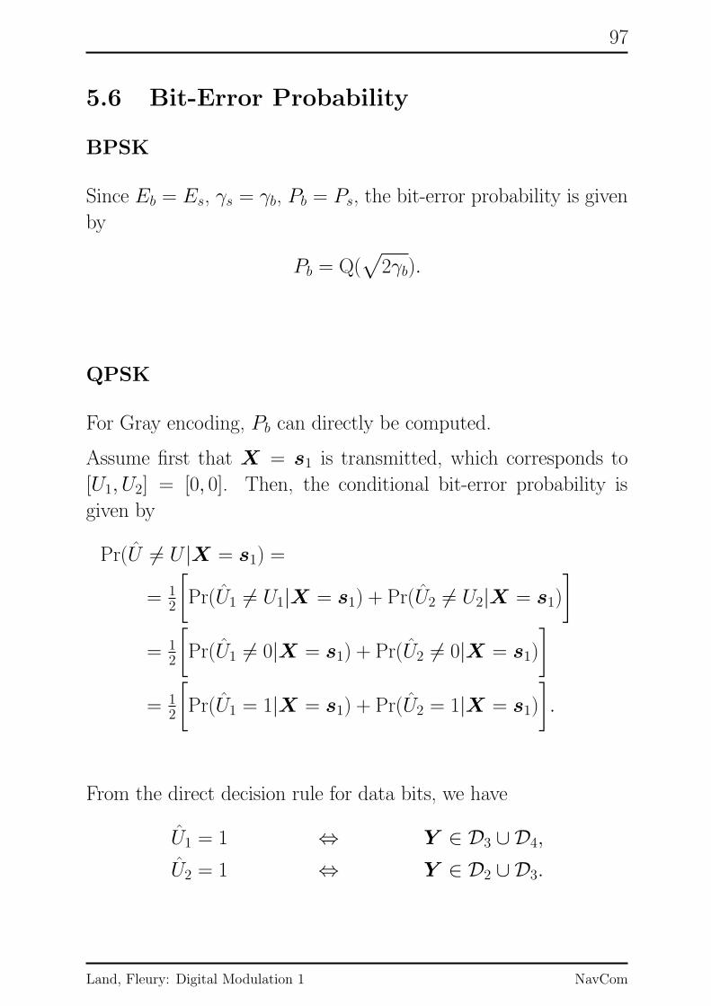
97
5.6 Bit-Error Probability
BPSK
Since Eb = Es, γs = γb, Pb = Ps, the bit-error probability is given
by
Pb = Q(√
2γb).
QPSK
For Gray encoding, Pb can directly be computed.
Assume first that X = s1 is transmitted, which corresponds to
[U1, U2] = [0, 0]. Then, the conditional bit-error probability is
given by
Pr(U 6= U |X = s1) =
= 12
[
Pr(U1 6= U1|X = s1) + Pr(U2 6= U2|X = s1)
]
= 12
[
Pr(U1 6= 0|X = s1) + Pr(U2 6= 0|X = s1)
]
= 12
[
Pr(U1 = 1|X = s1) + Pr(U2 = 1|X = s1)
]
.
From the direct decision rule for data bits, we have
U1 = 1 ⇔ Y ∈ D3 ∪ D4,
U2 = 1 ⇔ Y ∈ D2 ∪ D3.
Land, Fleury: Digital Modulation 1 NavCom

98
Thus,
Pr(U 6= U |X = s1) =
= 12
[
Pr(Y ∈ D3 ∪ D4) + Pr(Y ∈ D2 ∪ D3)
]
= 12
[
Pr(
W ′1 < −
√Es
2
)
+ Pr(
W ′2 >
√Es
2
)]
= 12
[
Pr(
W ′1√N0/2
< −√
Es
N0
)
+ Pr(
W ′2√N0/2
>√
Es
N0
)]
= Q(√γs).
By symmetry, all four conditional bit-error probabilities are iden-
tical. Since two data bits are transmitted per modulation sym-
bol (waveform) in QPSK, we have the relations Es = 2Eb and
γs = 2γb. Therefore,
Pb = Q(√
2γb).
(Remember: Pb ≈ 10−5 for γb ≈ 9.6 dB.)
Land, Fleury: Digital Modulation 1 NavCom

99
Comparison of QPSK and BPSK
(i) QPSK has exactly the same bit-error probability as BPSK.
(ii) Relation between symbol duration T and (average) bit dura-
tion Tb = T/K:
BPSK: T = Tb,
QPSK: T = 2Tb.
Hence, for a fixed symbol duration T , the bit rate of QPSK
is twice as fast as that of BPSK.
General Case
Since Gray encoding is used, we have
Pb ≈1
log2MPs
for high SNR.
The symbol-error probability may be determined using one of the
methods mentioned above.
Land, Fleury: Digital Modulation 1 NavCom

100
6 Offset Quadrature Phase-ShiftKeying (OQPSK)
Offset QPSK is a variant of QPSK. It has the same performance
as QPSK, but the requirements on the transmitter and receiver
hardware are lower.
6.1 Signaling Scheme
Consider QPSK with the following “tilted” signal constella-
tion and Gray encoding:PSfrag replacements
√Es
√
Es/2ψ1
ψ2
0001
1011
The phase of QPSK can change by maximal π. This is the case
for instance, when two consecutive 2-bit blocks are [00], [11] or
[01], [10]. These phase changes put high requirements on the dy-
namic behavior of the RF-part of the QPSK transmitter and re-
ceiver.
Phase changes of π can be avoided by staggering the quadrature
branch of QPSK by T/2 = Tb. The resulting modulation scheme
is called staggered QPSK or offset QPSK (OQPSK).
Land, Fleury: Digital Modulation 1 NavCom

101
Without significant loss of generality, we assume
f0 =2L
Tfor some L� 1, L ∈ N.
Remark
The ψ1 component of the modulation symbol is called the in-phase
component (I), and the ψ2 component is called the quadrature
component (Q).
6.2 Transceiver
We consider communication over an AWGN channel.
PSfrag replacements
Vector
Vector
Encoder
Decoder
AWGN Vector Channel
[U1, U2] X(t)X1
X2
W (t)
Y (t)
Y1
Y2
[U1, U2]
T
T2
3T2
√2
T
√2
T
cos 2πf0t
cos 2πf0t
− sin 2πf0t
− sin 2πf0t
√2
T
∫ T
0(.)dt
√2
T
∫3T/2
T/2(.)dt
Land, Fleury: Digital Modulation 1 NavCom

102
6.3 Phase Transitions for QPSK andOQPSK
Example: Transmission of three symbols
For the transmission of three symbols, we consider the data bits
u = [u1, u2], the in-phase component (I) and the quadrature com-
ponent (Q) of the modulation symbol, and the phase change ∆φ.
For convenience, let a :=√
Es/2.
QPSK
PSfrag replacements
u 00 01
10
11
I
Q
∆φ
0 TT2 = Tb 2T 3T
t
+a+a
+a −a−a−a
+π−π+π
2
−π2
OQPSK
PSfrag replacements
u 00 01
10
11
I
Q
∆φ 0
0 TT2 = Tb 2T 3T
t
+a+a
+a
+a+a
+a
−a−a−a
−a−a−a
+π
−π+π
2+π2 −π
2
3
Land, Fleury: Digital Modulation 1 NavCom

103
QPSK exhibits phase changes {±π2 ,±π} at times that are mul-
tiples of the signaling interval T . In contrast to this, OQPSK
exhibits phase changes {±π2} at times that are multiples of the bit
duration Tb = T/2.
Remarks
(i) OQPSK has the same bit-error probability as QPSK.
(ii) Staggering the quadrature component of QPSK by T/2 does
not prevent phase changes of π if the signaling constellation
of QPSK is not tilted. (Why?)
Land, Fleury: Digital Modulation 1 NavCom

104
7 Frequency-Shift Keying (FSK)
In FSK, the waveforms are sines, and the information is conveyed
by the frequencies of the waveforms. FSK with two waveforms is
called binary FSK (BFSK), and FSK with M waveforms is called
M -ary FSK (MFSK).
7.1 BFSK with Coherent Demodulation
7.1.1 Signal Waveforms
Set S of two sinus waveforms with different frequencies f1, f2 and
(possibly) different but known phases φ1, φ2 ∈ [0, 2π):
s1(t) =√
2P cos(2πf1t + φ1
),
s2(t) =√
2P cos(2πf2t + φ2
).
Both values are limited to the time interval t ∈ [0, T ]. Thus we
have
S ={s1(t), s2(t)
}.
Usually, f1, f2 � 1/T . To simplify the theoretical analysis, we
assume that
f1 =k1
T, f2 =
k2
T,
where k1, k2 ∈ N and k1, k2 � 1.
Both waveforms have the same energy
Es =
∞∫
−∞
s21(t)dt =
∞∫
−∞
s22(t)dt = PT.
Land, Fleury: Digital Modulation 1 NavCom

105
We assume the following BFSK transmitter:
{0, 1} → S
u 7→ x(t)
with the mapping
0 7→ s1(t)
1 7→ s2(t).
The frequency separation
∆f = |f1 − f2|
is selected such that s1(t) and s2(t) are orthogonal, i.e.,
〈s1(t), s2(t)〉 =
T∫
0
s1(t)s2(t)dt = 0.
The necessary condition for orthogonality is
∆f =k
T
with k ∈ N. Notice that the minimum frequency separation is
1/T .
The phases are assumed to be known to the receiver. Demodula-
tion with phase information (known phases or estimated phases)
is called coherent demodulation.
Land, Fleury: Digital Modulation 1 NavCom

106
7.1.2 Signal Constellation
Orthonormal functions:
ψ1(t) = 1√Ess1(t) =
√2T cos
(2πf1t + φ1
)
ψ2(t) = 1√Ess2(t) =
√2T cos
(2πf2t + φ2
)
for t ∈ [0, T ].
Geometrical representation of the waveforms:
s1(t) =√
Es · ψ1(t) + 0 · ψ2(t) ←→ s1 = (√
Es, 0)T
s2(t) = 0 · ψ1(t) +√
Es · ψ2(t) ←→ s1 = (0,√
Es)T.
Signal constellation:
PSfrag replacements
00
√Es
√Es
√2Es
ψ1
ψ2
s1
s2
D1
D2
BFSK with coherent demodulation has the same signal constella-
tion as BPPM.
Accordingly, these two modulation methods are equivalent.
Land, Fleury: Digital Modulation 1 NavCom

107
7.1.3 ML Decoding
ML symbol decision rule
decML(y) = argminx∈{s1,s2}
‖y − x‖2 =
{
(√Es, 0)T for y1 ≥ y2,
(0,√Es)
T for y1 < y2.
Decision regions
D1 = {y ∈ R2 : y1 ≥ y2}, D2 = {y ∈ R
2 : y1 < y2}.
PSfrag replacements
00
√Es
√Es
√2Es
y1
y2
s1
s2 D1
D2
(u = 0)
(u = 1)
ML decoder for BFSK
u = enc-1(decML(y)) =
{
0 for y1 ≥ y2,
1 for y1 < y2.
Implementation of the ML decoder
PSfrag replacements
UY1
Y2
Z z ≥ 0→ 0
z < 0→ 1
Land, Fleury: Digital Modulation 1 NavCom
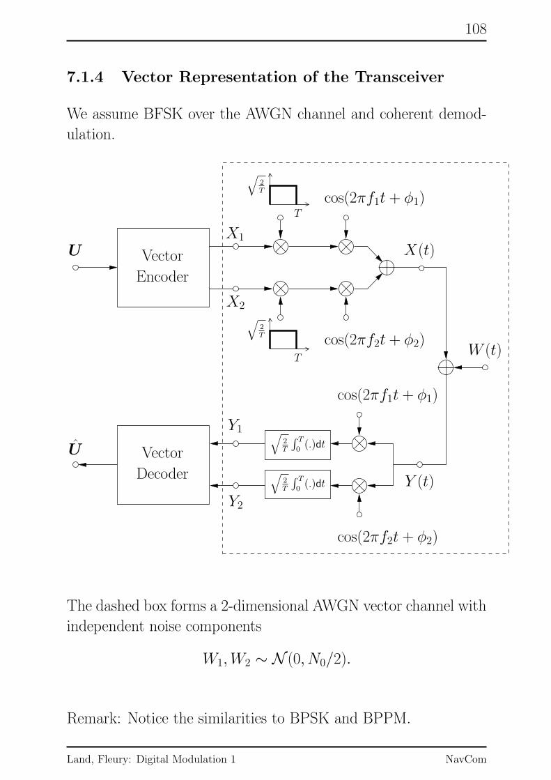
108
7.1.4 Vector Representation of the Transceiver
We assume BFSK over the AWGN channel and coherent demod-
ulation.
PSfrag replacements
Vector
Vector
Encoder
Decoder
AWGN Vector ChannelU X(t)
X1
X2
W (t)
Y (t)
Y1
Y2
U
T
T
√2
T
√2
T
cos(2πf1t + φ1)
cos(2πf1t + φ1)
cos(2πf2t + φ2)
cos(2πf2t + φ2)
√2
T
∫ T
0(.)dt
√2
T
∫ T
0(.)dt
The dashed box forms a 2-dimensional AWGN vector channel with
independent noise components
W1,W2 ∼ N (0, N0/2).
Remark: Notice the similarities to BPSK and BPPM.
Land, Fleury: Digital Modulation 1 NavCom

109
7.1.5 Error Probabilities
As the signal constellation of coherently demodulated BFSK is the
same as that of BPPM, the error probabilities are the same:
Ps = Q(√γs),
Pb = Q(√γb).
For the derivation, see analysis of BPPM.
Land, Fleury: Digital Modulation 1 NavCom

110
7.2 MFSK with Coherent Demodulation
7.2.1 Signal Waveforms
The signal waveforms are
sm(t) =
{√2P cos
(2πfmt + φm
)for t ∈ [0, T ],
0 elsewhere,
m = 1, 2, . . . ,M .
The parameters of the waveforms are as follows:
(a) frequencies fm = km/T for km ∈ N and km � 1;
(b) frequency separations ∆fm,n = |fm − fn| = km,n/T , km,n ∈N;
(c) phases φm ∈ [0, 2π);
m,n = 1, 2, . . . ,M .
The phases are assumed to be known to the receiver. Thus, we
consider coherent demodulation.
As in the binary case, all waveforms have the same energy
Es =
∞∫
−∞
s2m(t)dt = PT.
Land, Fleury: Digital Modulation 1 NavCom

111
7.2.2 Signal Constellation
Orthonormal functions:
ψm(t) = 1√Essm(t) =
√2T cos
(2πfmt + φm
)
for t ∈ [0, T ], m = 1, 2, . . . ,M .
Geometrical representation of the waveforms:
s1(t) =√
Es · ψ1(t) ←→ s1 = (
M elements︷ ︸︸ ︷√
Es, 0, . . . , 0)T
...
sM(t) =√
Es · ψM(t) ←→ s1 = (0, . . . , 0,√
Es)T.
MFSK with coherent demodulation has the same signal constella-
tion as MPPM.
Accordingly, these two modulation methods are equivalent and
have the same performance.
Vector Encoder
enc : u = [u1, . . . , uK ] 7→ x = enc(u)
U = {0, 1}K → X ={s1, s2, . . . , sM
}
with K = log2M .
Land, Fleury: Digital Modulation 1 NavCom

112
7.2.3 Vector Representation of the Transceiver
We assume MFSK over the AWGN channel and coherent demod-
ulation.
PSfrag replacements
Vector
Vector
Encoder
Decoder
AWGN Vector ChannelU X(t)
X1
XM
W (t)
Y (t)
Y1
YM
U
T
T
√2
T
√2
T
cos(2πf1t + φ1)
cos(2πf1t + φ1)
cos(2πfMt + φM)
cos(2πfMt + φM)
√2
T
∫ T
0(.)dt
√2
T
∫ T
0(.)dt
The dashed box forms an M -dimensional AWGN vector channel
with mutually independent components
Wm ∼ N (0, N0/2),
m = 1, 2, . . . ,M .
Land, Fleury: Digital Modulation 1 NavCom
113
Remarks
The M waveforms sm(t) ∈ S are orthogonal. The receiver simply
correlates the received waveform y(t) to each of the possibly trans-
mitted waveforms sm(t) ∈ S and selects the one with the highest
correlation as the estimate.
7.2.4 Error Probabilities
The signal constellation of coherently demodulated MFSK is the
same as that of MPPM. Therefor, the symbol-error probability
and the bit-error probability are the same. For the analysis, see
MPPM.
Land, Fleury: Digital Modulation 1 NavCom

114
7.3 BFSK with Noncoherent Demodulation
7.3.1 Signal Waveforms
The signal waveforms are
s1(t) =√
2P cos(2πf1t + φ1
),
s2(t) =√
2P cos(2πf2t + φ2
).
for t ∈ [0, T ) with
(i) frequencies fm = km/T for km ∈ N and km � 1, m = 1, 2,
and
(ii) frequency separation ∆f = |f1−f2| = k/T for some k ∈ N.
As opposed to the case of coherent demodulation, the phases φ1
and φ2 are not known to the receiver. Instead, they are assumed
as random variables that are uniformly distributed, i.e.,
pΦ1(φ1) =1
2π, pΦ2(φ2) =
1
2π
for φ1, φ2 ∈ [0, 2π).
Demodulation without use of phase information is called nonco-
herent demodulation. As the phases need not be estimated,
the noncoherent demodulator has a lower complexity than the co-
herent demodulator.
Land, Fleury: Digital Modulation 1 NavCom

115
7.3.2 Signal Constellation
Using the same method as for the canonical decomposition of PSK,
the orthonormal functions are obtained as
ψ1(t) =√
2T cos
(2πf1t
)
ψ2(t) = −√
2T sin
(2πf1t
)
ψ3(t) =√
2T cos
(2πf2t
)
ψ4(t) = −√
2T sin
(2πf2t
)
for t ∈ [0, T ].
(Remember: cos(x + y) = cosx cos y − sinx sin y.)
Geometrical representations of the waveforms:
s1(t) =√
Es cosφ1 · ψ1(t) +√
Es sinφ1 · ψ2(t)
←→ s1 =(√
Es cosφ1,√
Es sinφ1, 0, 0)T,
s2(t) =√
Es cosφ2 · ψ3(t) +√
Es sinφ2 · ψ4(t)
←→ s2 =(0, 0,
√
Es cosφ2,√
Es sinφ2
)T.
The signal constellation is thus
X ={s1, s2
}.
The transmitted (modulation) symbols are the four-
dimensional(!) vectors
X =(X1, X2︸ ︷︷ ︸
“for s1”
, X3, X4︸ ︷︷ ︸
“for s2”
)T ∈ X.
Land, Fleury: Digital Modulation 1 NavCom

116
7.3.3 Noncoherent Demodulator
As there are four orthonormal basis functions, the demodulator
has four branches:
PSfrag replacements
Y (t)
Y1
Y2
Y3
Y4
√2
T
∫ T
0(.)dt
√2
T
∫ T
0(.)dt
√2
T
∫ T
0(.)dt
√2
T
∫ T
0(.)dt
cos 2πf1t
− sin 2πf1t
cos 2πf2t
− sin 2πf2t
Notice the similarity to PSK.
We introduce the vectors
Y 1 =
(Y1
Y2
)
, Y 2 =
(Y3
Y4
)
and
Y =(Y T
1 ,YT2
)T=(Y1, Y2, Y3, Y4
)T.
(Loosly speaking, Y 1 corresponds to s1 and Y 2 corresponds to s2.)
Land, Fleury: Digital Modulation 1 NavCom

117
7.3.4 Conditional Probability of Received Vector
Assume that the transmitted vector is
X = s1 =(√
Es cosφ1,√
Es sinφ1, 0, 0)T.
Then, the received vector is
Y =(√
Es cosφ1 +W1,√
Es sinφ1 +W2︸ ︷︷ ︸
Y T1
,W3,W4︸ ︷︷ ︸
Y T2
)T
=(Y T
1 ,YT2
)T.
The conditional probability density of Y given X = s1 and φ1 is
pY |X,Φ1(y|s1, φ1) =
=(
1πN0
)2 · exp(− 1N0‖y − s1‖2
)
=(
1πN0
)2 · exp(
− 1N0
[(y1 −
√
Es cosφ1
)2+
+(y2 −
√
Es sinφ1
)2+ y2
3 + y24
])
=(
1πN0
)2 · exp(−Es
N0
)· exp
(
− 1N0
[
‖y1‖2 + ‖y2‖2])
·
· exp(
2√Es
N0
(y1 cosφ1 + y2 sinφ1
))
With α1 = tan−1(y2/y1), we may write
y1 cosφ1 + y2 sinφ1 = ‖y1‖(cosα1 cosφ1 + sinα1 sinφ1
)
= ‖y1‖ cos(φ1 − α1).
Land, Fleury: Digital Modulation 1 NavCom

118
The phase can be removed from the condition by averaging over
it. The phase is uniformly distributed in [0, 2π), and thus
pY |X(y|s1) =
=
2π∫
0
pY |X,Φ1(y|s1, φ1) pφ1(φ1) dφ1
= 12π
2π∫
0
pY |X,Φ1(y|s1, φ1) dφ1
= 12π
2π∫
0
(1
πN0
)2 · exp(−Es
N0
)· exp
(
− 1N0
[
‖y1‖2 + ‖y2‖2])
·
· exp(
2√Es
N0‖y1‖ cos(φ1 − α1)
)
dφ1
=(
1πN0
)2 · exp(−Es
N0
)· exp
(
− 1N0
[
‖y1‖2 + ‖y2‖2])
·
· 12π
2π∫
0
exp(
2√Es
N0‖y1‖ cos(φ1 − α1)
)
dφ1
︸ ︷︷ ︸
I0(
2√Es
N0‖y1‖
)
.
The above function is the modified Bessel function of order 0, and
it is defined as
I0(v) := 12π
2π∫
0
exp(v cos(φ− α)
)dφ
for α ∈ [0, 2π). It is monotonically increasing. A plot can be found
in [1, p. 403].
Land, Fleury: Digital Modulation 1 NavCom

119
Combining all the above results yields
pY |X(y|s1) =(
1πN0
)2 · exp(−Es
N0
)·
· exp(
− 1N0
[
‖y1‖2 + ‖y2‖2])
· I0(
2√Es
N0‖y1‖
).
Using the same reasoning, we obtain
pY |X(y|s2) =(
1πN0
)2 · exp(−Es
N0
)·
· exp(
− 1N0
[
‖y1‖2 + ‖y2‖2])
· I0(
2√Es
N0‖y2‖
).
7.3.5 ML Decoding
Remember the definitions
Y =(Y1, Y2︸ ︷︷ ︸
Y 1
, Y3, Y4︸ ︷︷ ︸
Y 2
)T=(Y T
1 ,YT2
)T.
ML symbol decision rule
x = decML(y) = argmaxx∈X
pY |X(y|x)
Let x = sm. Then, the index of the ML vector is
m = argmaxm∈{1,2}
I0(
2√Es
N0‖ym‖
)
= argmaxm∈{1,2}
‖ym‖
= argmaxm∈{1,2}
‖ym‖2.
Notice that selecting x and selecting m are equivalent.
Land, Fleury: Digital Modulation 1 NavCom

120
ML decoder
u =
{
0 for x = s1 ⇔ ‖y1‖ ≥ ‖y2‖,1 for x = s2 ⇔ ‖y1‖ < ‖y2‖.
Optimal noncoherent receiver for BFSKPSfrag replacements
Y (t)
Y1
Y2
Y3
Y4
‖Y 1‖2
‖Y 2‖2
Z U
√2
T
∫ T
0(.)dt
√2
T
∫ T
0(.)dt
√2
T
∫ T
0(.)dt
√2
T
∫ T
0(.)dt
cos 2πf1t
− sin 2πf1t
cos 2πf2t
− sin 2πf2t
(.)2
(.)2
(.)2
(.)2
z ≥ 0→ 0
z < 0→ 1
Notice:
‖Y 1‖2 =√
Y 21 + Y 2
2 , Z = ‖Y 1‖2 − ‖Y 2‖2,
‖Y 2‖2 =√
Y 23 + Y 2
4 .
Land, Fleury: Digital Modulation 1 NavCom
121
7.4 MFSK with Noncoherent Demodula-tion
7.4.1 Signal Waveforms
The signal waveforms are
sm(t) =√
2P cos(2πfmt + φm
)
for t ∈ [0, T ), m = 1, 2, . . . ,M , with
(i) fm = km/T for km ∈ N and km � 1, m = 1, 2, . . . ,M ,
(ii) ∆fm, n = |fm − fn| = k/T for some km,n ∈ N, m,n =
1, 2, . . . ,M .
The phases φ1, φ2, . . . , φM are not known to the receiver. They
are assumed to be uniformly distributed in [0, 2π).
Land, Fleury: Digital Modulation 1 NavCom
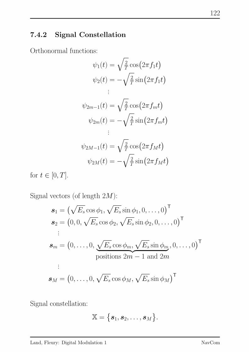
122
7.4.2 Signal Constellation
Orthonormal functions:
ψ1(t) =√
2T cos
(2πf1t
)
ψ2(t) = −√
2T sin
(2πf1t
)
...
ψ2m−1(t) =√
2T cos
(2πfmt
)
ψ2m(t) = −√
2T sin
(2πfmt
)
...
ψ2M−1(t) =√
2T cos
(2πfMt
)
ψ2M(t) = −√
2T sin
(2πfMt
)
for t ∈ [0, T ].
Signal vectors (of length 2M):
s1 =(√
Es cosφ1,√
Es sinφ1, 0, . . . , 0)T
s2 =(0, 0,
√
Es cosφ2,√
Es sinφ2, 0, . . . , 0)T
...
sm =(0, . . . , 0,
√
Es cosφm,√
Es sinφm︸ ︷︷ ︸
positions 2m− 1 and 2m
, 0, . . . , 0)T
...
sM =(0, . . . , 0,
√
Es cosφM ,√
Es sinφM)T
Signal constellation:
X ={s1, s2, . . . , sM
}.
Land, Fleury: Digital Modulation 1 NavCom

123
7.4.3 Conditional Probability of Received Vector
Using the same reasoning as for BFSK, we can show that
pY |X(y|sm) =(
1πN0
)M · exp(−Es
N0
)·
· exp(
− 1N0
M∑
m=1
‖ym‖2)
· I0(
2√Es
N0‖ym‖
)
with the definition
Y =(Y1, Y2︸ ︷︷ ︸
Y 1
, Y3, Y4︸ ︷︷ ︸
Y 2
, . . . , Y2M−1, Y2M︸ ︷︷ ︸
Y M
,)T
=(Y T
1 ,YT2 , . . . ,Y
TM
)T.
7.4.4 ML Decision Rule
Original ML decision rule:
x = decML(y) = argmaxx∈X
pY |X(y|x)
Let x = sm. Then, the original decision rule may equivalently be
expressed as
m = argmaxm∈{1,...,M}
‖ym‖2.
Land, Fleury: Digital Modulation 1 NavCom

124
7.4.5 Optimal Noncoherent Receiver for MFSK
Remember: “noncoherent demodulation” means that no phase in-
formation is used for demodulation.
The optimal noncoherent receiver for MFSK over the AWGN chan-
nel is as follows:
PSfrag replacements
Y (t)
Y1
Y2
Y2M−1
Y2M
‖Y 1‖2
‖Y M‖2
U
√2
T
∫ T
0(.)dt
√2
T
∫ T
0(.)dt
√2
T
∫ T
0(.)dt
√2
T
∫ T
0(.)dt
cos 2πf1t
− sin 2πf1t
cos 2πfM t
− sin 2πfM t
(.)2
(.)2
(.)2
(.)2
select
maximum
and
compute
encoder
inverse
Notice that U = [U1, . . . , UK ] with K = log2M .
Land, Fleury: Digital Modulation 1 NavCom

125
7.4.6 Symbol-Error Probability
Assume that X = s1 is transmitted. Then, the probability of a
correct decision is
Pr(X = X|X = s1) =
= Pr(‖Y m‖2 ≤ ‖Y 1‖2 for all m 6= 1|X = s1
).
Provided that X = s1 is transmitted, we have
Y 1 =(√
Es cosφ1 +W1,√
Es sinφ1 +W2
)T
Y 2 =(W3,W4
)T= W 2
...
Y m =(W2m−1,W2m
)T= Wm
...
Y M =(W2M−1,W2M
)T= WM .
Consequently,
Pr(X = X|X = s1) =
= Pr(‖Wm‖2 ≤ ‖Y 1‖2 for all m 6= 1|X = s1
)
= Pr(
1√N0/2‖Wm‖2
︸ ︷︷ ︸
Rm
≤ 1√N0/2‖Y 1‖2
︸ ︷︷ ︸
R1
for all m 6= 1|X = s1
)
= Pr(Rm ≤ R1 for all m 6= 1|X = s1
)
=
∞∫
0
Pr(Rm ≤ R1 for all m 6= 1|X = s1, R1 = r1
)·
· pR1(r1) dr1.
Land, Fleury: Digital Modulation 1 NavCom

126
The probability density function of R1 is denoted by pR1(r1).
The probability of a correct decision can further be written as
Pr(X = X|X = s1) =
=
∞∫
0
Pr(Rm ≤ r1 for all m 6= 1|X = s1, R1 = r1
)pR1(r1) dr1
=
∞∫
0
Pr(Rm ≤ r1 for all m 6= 1
)pR1(r1) dr1
The noise vectors W2, . . . ,WM are mutually statistically indepen-
dent, and thus also the values R2, . . . , RM are mutually statisti-
cally independent. Therefore,
Pr(X = X|X = s1) =
∞∫
0
M∏
m=2
Pr(Rm ≤ r1) pR1(r1) dr1
=
∞∫
0
(
Pr(R2 ≤ r1))M−1
pR1(r1) dr1.
Notice that
Pr(Rm ≤ r1) = Pr(R2 ≤ r1)
for m = 2, 3, . . . ,M , because R2, . . . , RM are identically dis-
tributed.
Land, Fleury: Digital Modulation 1 NavCom

127
The conditional probability of a symbol-error can thus be written
as
Pr(X 6= X|X = s1) = 1− Pr(X = X|X = s1)
= 1−∞∫
0
(
Pr(R2 ≤ r1))M−1
pR1(r1) dr1.
By symmetry, all conditional symbol-error probabilities are the
same. Thus,
Ps = 1−∞∫
0
(
Pr(R2 ≤ r1))M−1
pR1(r1) dr1.
In the above expressions, we have the following distributions (see
literature):
(i) R2 (and also R3, . . . , RM) is Rayleigh distributed:
pR2(r2) = r2 e−r22/2.
Accordingly, its cumulative distribution function results as
Pr(R2 ≤ r1) = 1− e−r21/2
(ii) R1 is Rice distributed:
pR1(r1) = r1 · exp(−1
2(r1 + 2γs)2)· I0(√
2γsr1)
Remark
The Rayleigh distribution and the Ricd distribution are often used
to model mobile radio channels.
Land, Fleury: Digital Modulation 1 NavCom

128
Using the first relation, we can expand the first term as
(
Pr(R2 ≤ r1))M−1
=(
1− e−r21/2)M−1
=
M−1∑
m=0
(−1)m(M − 1
m
)
e−mr21/2
After integrating over r1, we obtain the following closed-form so-
lution for the symbol-error probability of MFSK with
noncoherent demodulation:
Ps =
M−1∑
m=1
(−1)m+1
(M − 1
m
)1
m + 1exp(
− m
m + 1γs
)
.
For M = 2, this sum simplifies to
Ps = 12 e−γs/2.
Land, Fleury: Digital Modulation 1 NavCom

129
7.4.7 Bit-Error Probability
BFSK
We have γb = γs and Pb = Ps.
Therefore, the bit-error probability is given by
Pb = 12 e−γb/2.
MFSK
For M > 2, we have
(i) γb = 1Kγs,
(ii) Pb =2K−1
2K − 1Ps with K = log2M (see MPPM).
Therefore the bit-error probability results as
Pb =2K−1
2K − 1
M−1∑
m=1
(−1)m+1
(M − 1
m
)1
m + 1exp(
− mK
m + 1γs
)
.
Plots of the error probability can be found in [1, p. 433].
Land, Fleury: Digital Modulation 1 NavCom

130
8 Minimum-Shift Keying (MSK)
MSK is a binary modulation scheme with coherent detection, and
it is similar to BFSK with coherent detection. The waveforms
are sines, the information is conveyed by the frequencies of the
waveforms, and the phases of the waveforms are chosen such that
there are no phase discontinuities. Thus, the power spectrum of
MSK is more compact than that of BFSK. The description of MSK
follows [2].
8.1 Motivation
Consider BFSK. The signal waveforms of BFSK are
U = 0 7→ s1(t) =√
2P cos(2πf1t
),
U = 1 7→ s2(t) =√
2P cos(2πf2t
),
for t ∈ [0, T ]. The minimum frequency separation such that s1(t)
and s2(t) are orthogonal (assuming coherent detection) is
∆f = |f1 − f2| =1
2T.
In the following, we assume minimum frequency separation.
Without loss of generality, we assume that
f1 =k
T, f2 =
k
T+
1
2T=k + 1/2
T,
for k ∈ N and k � 1, i.e., k is a large integer. Thus, we have the
following properties:
waveform number of periods in t ∈ [0, T )
s1(t) k
s2(t) k + 1/2
Land, Fleury: Digital Modulation 1 NavCom

131
Example: Output of BFSK Transmitter
Consider BFSK with f1 = 1/T and f2 = 3/2T such that the fre-
quency separation ∆ = 1/T is minimum. Assume the bit sequence
U [0,4] = [U0, U1, U2, U3, U4] = [0, 1, 1, 0, 0].
The resulting output signal x•(t) of the BFSK transmitter shows
discontinuities. 3
The discontinuities produce high side-lobes in the power spectrum
of X(t), which is either inefficient or problematic. This can be
avoided by slightly modifying the modulation scheme.
We rewrite the signal waveforms as follows:
s1(t) =√
2P cos(2πf1t
),
s2(t) =√
2P cos(2πf1t + 2π
t
2T
),
for t ∈ [0, T ]. (Remember that f2 = f1 + 1/2T .) Thus, we can
express the output signal as
x(t) =√
2P cos(2πf1t + φ•(t)
),
t ∈ [0, T ), with the phase function
φ•(t) =
{
0 for s1(t),
2π t2T for s2(t).
Notice that φ•(t) depends directly on the transmitted source bit U .
Land, Fleury: Digital Modulation 1 NavCom

132
Example: Phase function of BFSK
The phase function φ•(t) of the previous example shows disconti-
nuities. 3
The discontinuities of the phase and thus of x(t) can be avoided by
making the phase continuous. This can be achieved by disabling
the “reset to zero” of φ•(t), yielding the new phase function φ(t).
Notice that this introduces memory in the transmitter.
Example: Modified BFSK Transmitter
(We continue the previous example.) The phase function φ(t) of
the modified transmitter is continuous. Accordingly, also the sig-
nal x(t) generated by the modified transmitter is continuous. 3
FSK with phase made continuous as described above is called
continuous-phase FSK (CPFSK). Binary CPFSK with minimum
frequency separation is termed minimum-shift keying (MSK).
8.2 Transmit Signal
The continuous-phase output signal of an MSK transmitter con-
sists of the following waveforms (the expressions on the right-hand
side are only used as abbreviations in the following):
s1(t) = +√
2P cos(2πf1t
)“f1”
s2(t) = −√
2P cos(2πf1t
)“−f1”
s3(t) = +√
2P cos(2πf2t
)“f2”
s4(t) = −√
2P cos(2πf2t
)“−f2”
t ∈ [0, T ].
Land, Fleury: Digital Modulation 1 NavCom
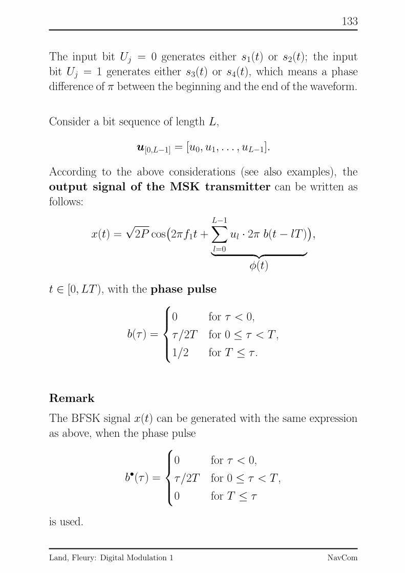
133
The input bit Uj = 0 generates either s1(t) or s2(t); the input
bit Uj = 1 generates either s3(t) or s4(t), which means a phase
difference of π between the beginning and the end of the waveform.
Consider a bit sequence of length L,
u[0,L−1] = [u0, u1, . . . , uL−1].
According to the above considerations (see also examples), the
output signal of the MSK transmitter can be written as
follows:
x(t) =√
2P cos(2πf1t +
L−1∑
l=0
ul · 2π b(t− lT )
︸ ︷︷ ︸
φ(t)
),
t ∈ [0, LT ), with the phase pulse
b(τ ) =
0 for τ < 0,
τ/2T for 0 ≤ τ < T ,
1/2 for T ≤ τ .
Remark
The BFSK signal x(t) can be generated with the same expression
as above, when the phase pulse
b•(τ ) =
0 for τ < 0,
τ/2T for 0 ≤ τ < T ,
0 for T ≤ τ
is used.
Land, Fleury: Digital Modulation 1 NavCom

134
Plotting all possible trajectories of φ(t), we obtain the (tilted)
phase tree of MSK.
PSfrag replacements
t
φ(t)
f1
f1f1f1
f1f1f1f1f1
f2
f2f2f2
f2f2f2f2f2
−f1−f1
−f1−f1−f1−f1
−f2−f2
−f2−f2−f2−f2
0
0 T 2T 3T 4T
5Tπ
2π
3π
4π
The physical phase is obtained by taking φ(t) modulo 2π. Plotting
all possible trajectories, we obtain the (tilted) physical-phase
trellis of MSK.
PSfrag replacements
t
φ(t) mod 2π
f1 f1f1f1f1
f2 f2f2f2f2
−f1−f1−f1−f1
−f2−f2−f2−f2
0
0 T 2T 3T 4T
5T
π
2π
Land, Fleury: Digital Modulation 1 NavCom

135
8.3 Signal Constellation
Signal waveforms:
s1(t) = +√
2P cos(2πf1t
),
s2(t) = −√
2P cos(2πf1t
),
s3(t) = +√
2P cos(2πf2t
),
s4(t) = −√
2P cos(2πf2t
),
t ∈ [0, T ].
Orthonormal functions:
ψ1(t) =√
2/T cos(2πf1t
),
ψ2(t) =√
2/T cos(2πf2t
),
t ∈ [0, T ].
Vector representation of the signal waveforms:
s1(t) = +√
Es ψ1(t) ←→ s1 = (+√
Es, 0)T
s2(t) = −√Es ψ1(t) ←→ s2 = (−√Es, 0)T = −s1
s3(t) = +√
Es ψ2(t) ←→ s3 = (0,+√
Es)T
s4(t) = −√Es ψ2(t) ←→ s4 = (0,−√Es)T = −s3
with Es = PT .
Land, Fleury: Digital Modulation 1 NavCom

136
Remark:
The modulation symbol at discrete time j is written as
Xj = (Xj,1, Xj,2)T.
For example, Xj = s1 means Xj,1 =√Es and Xj,2 = 0.
Signal constellation:
PSfrag replacements
ψ1
ψ2
s1s2
s3
s4
Remark:
MSK and QPSK have the same signal constellation. However, the
two modulation schemes are not equivalent because their vector
encoders are different. This is discussed in the following.
Land, Fleury: Digital Modulation 1 NavCom

137
Modulator:
The symbol Xj = (Xj,1, Xj,2)T is transmitted in the time interval
t ∈ [jT, (j + 1)T ).
This time interval can also be written as
t = jT + τ, τ ∈ [0, T ).
The modulation for τ = t − jT ∈ [0, T ), j = 0, 1, 2, . . . , is then
given by the mapping
Xj 7→ Xj(τ ),
and it can be implemented by
PSfrag replacements
Xj,1
Xj,2
Xj(τ )
T
T
√2
T
√2
T
cos(2πf1τ )
cos(2πf2τ )
Remark:
The index j is not necessary for describing the modulator. It is
only introduced to have the same notation as being used for the
vector encoder.
Land, Fleury: Digital Modulation 1 NavCom

138
8.4 A Finite-State Machine
Consider the following device (which is a simple finite-state ma-
chine)PSfrag replacements
Uj Vj
Vj+1
T
It consists of the following components:
(i) A modulo-2 adder:PSfrag replacements
Uj
Vj
Vj+1
It has the functionality
Vj+1 = Uj ⊕ Vj = Uj + Vj mod 2.
(ii) A shift register clocked at times T (“every T seconds”):
PSfrag replacements
Uj
VjVj+1 T
(iii) The sequence {Uj} is a binary sequence with elements
in {0, 1}, and so is the sequence {Vj}.
The output value Vj describes the state of this device.
Land, Fleury: Digital Modulation 1 NavCom

139
As Vj ∈ {0, 1}, this device can be in two different states. All possi-
ble transitions can be depicted in a state transition diagram:
PSfrag replacements
0
1
0
0
0
1
11
The values in the circles denote the states v, and the labels of the
arrows denote the inputs u.
The state transitions and the associated input values can also be
depicted in a trellis diagram. The initial state is assumed to be
zero.
PSfrag replacements
000000
111111
0 0
0
0
0
0
0
0
0
1 1
1
1
1
1
1
1
1
0 1 2 3 4 5
The time indices are written below the states.
The emphasized path corresponds to the input sequence
[U0, U1, U2, U3, U4] = [0, 1, 1, 0, 0].
Land, Fleury: Digital Modulation 1 NavCom

140
8.5 Vector Encoder
According to the trellis of the physical phase, the initial phase at
the beginning of each symbol interval can take the two values 0
and π. These values determine the state of the encoder. We use
the following association:
phase 0 ↔ state V = 0,
phase π ↔ state V = 1.
The functionality of the encoder can be described by the following
state transition diagram:
PSfrag replacements 0
π
0/s1
0/s2
1/s3 1/s4
The transitions are labeled by u/x. The value u denotes the binary
source symbol at the encoder input, and x denotes the modulation
symbol at the encoder output.
Remember: s2 = −s1 and s4 = −s3.
Remark
The vector encoder is a finite-state machine as considered in the
previous section.
Land, Fleury: Digital Modulation 1 NavCom

141
The temporal behavior of the encoder can be described by the
trellis diagram:
PSfrag replacements
000000
ππππππ
0/s10/s10/s10/s1 0/s1
0/s20/s20/s20/s2
1/s 3
1/s 3
1/s 3
1/s 3
1/s 3
1/s4
1/s4
1/s4
1/s4
0 1 2 3 4 5
The emphasized path corresponds to the input sequence
[U0, U1, U2, U3, U4] = [0, 1, 1, 0, 0].
General Conventions
(i) The input sequence of length L is written as
u = [u0, u1, . . . , uL−1].
(ii) The initial state is V0 = 0.
(iii) The final state is VL = 0.
The last bit UL−1 is selected such that the encoder is driven back
to state 0:
VL−1 = 0 −→ UL−1 = 0,
VL−1 = 1 −→ UL−1 = 1.
Therefore, UL−1 does not carry information.
Land, Fleury: Digital Modulation 1 NavCom

142
Generation of the Encoder Outputs
Consider one trellis section:PSfrag replacements
00
ππ
0/s1
0/s2
1/s 3
1/s4
j j + 1
Remember: s2 = −s1 and s4 = −s3.
Observations:
(i) Input symbols → output vectors
Uj = 0 −→ Xj ∈ {s1, s2} = {s1,−s1},Uj = 1 −→ Xj ∈ {s3, s4} = {s3,−s3}.
(ii) Encoder state → output vectors
Vj = 0 (“0”) −→ Xj ∈ {s1, s3}Vj = 1 (“π”) −→ Xj ∈ {s2, s4} = {−s1,−s3}.
Using these observations, the above device can be supplemented
to obtain an implementation of the vector encoder for MSK.
Land, Fleury: Digital Modulation 1 NavCom

143
Block Diagram of the Vector Encoder for MSK
PSfrag replacements
Uj
UjVjVj+1
Xj,1
Xj,2T
UjVj
s1
s2
s3
s4
00
01
10
11
At time index j:
• input symbol Uj,
• state Vj,
• output symbol X j = (Xj,1, Xj,2)T,
• subsequent state Vj+1.
Notice:
(i) Uj controls the frequency of the transmitted waveform.
(ii) Vj controls the polarity of the transmitted waveform.
Land, Fleury: Digital Modulation 1 NavCom

144
8.6 Demodulator
The received symbol Y j = (Yj,1, Yj,2)T is determined in the time
interval
t ∈ [jT, (j + 1)T ).
This time interval can also be written as
t = jT + τ, τ ∈ [0, T ).
The demodulation for τ = t − jT ∈ [0, T ), j = 0, 1, 2, . . . , can
then be implemented as follows:PSfrag replacements
Y (t)
Yj,1
Yj,2
T√2
T
cos(2πf1τ )
cos(2πf2τ )
√2
T
∫ T
0(.)dτ
√2
T
∫ T
0(.)dτ
Land, Fleury: Digital Modulation 1 NavCom

145
8.7 Conditional Probability Density of Re-ceived Sequence
Sequence of (two-dimensional) received symbols
[Y 0, . . . ,Y L−1] = [X0 + W 0, . . . ,XL−1 + W L−1].
The vector [W 0, . . . ,W L−1] is a white Gaussian noise sequence
with the properties:
(i) W 0, . . . ,W L−1 are independent ;
(ii) each (two-dimensional) noise vector is distributed as
W j =
[Wj,1
Wj,2
]
∼ N([0
0
]
,
[N0/2 0
0 N0/2
])
Illustration of the AWGN vector channel:
PSfrag replacements
Xj
Xj,1
Xj,2
W jWj,1
Wj,2
Y j
Yj,1
Yj,2
Land, Fleury: Digital Modulation 1 NavCom

146
Conditional probability of y[0,L−1] = [y0, . . . ,yL−1] given that
x[0,L−1] = [x0, . . . ,xL−1] was transmitted:
pY [0,L−1]|X [0,L−1]
(y0, . . . ,yL−1|x0, . . . ,xL−1
)=
=
L−1∏
j=0
pY j |Xj
(yj|xj
)
=
L−1∏
j=0
[ 1
πN0· exp
(− 1N0‖yj − xj‖2
)]
=( 1
πN0
)L
· exp(− 1N0
L−1∑
j=0
‖yj − xj‖2).
Notice that this is the likelihood function of x[0,L−1] for a given
received sequence y[0,L−1].
8.8 ML Sequence Estimation
The trellis of the vector encoder has the following two properties:
(i) Each input sequence u[0,L−1] = [u0, . . . , uL−1] uniquely de-
termines a path of length L in the trellis, and vice versa.
(ii) Each path in the trellis uniquely determines an output se-
quence x[0,L−1] = [x0, . . . ,xL−1]
A sequence x[0,L−1] of length L generated by the vector encoder is
called an admissible sequence if the initial and the final state of
the encoder are zero, i.e., if V0 = VL = 0. The set of admissible
sequences is denoted by A.
Land, Fleury: Digital Modulation 1 NavCom

147
Using these definitions, the ML decoding rule is the following:
Search the trellis for an admissible sequence that max-
imizes the likelihood function.
Or in mathematical terms:
x[0,L−1] = argmaxx[0,L−1]∈A
p(y[0,L−1]|x[0,L−1]).
Using the relation
‖yj − xj‖2 = ‖yj‖2︸ ︷︷ ︸
indep. of xj
−2〈yj,xj〉 + ‖xj‖2︸ ︷︷ ︸
= Es
and the expression for the likelihood function, the rule for ML
sequence estimation (MLSE) can equivalently be formulated
as follows:
x[0,L−1] = argmaxx[0,L−1]∈A
exp(− 1
N0
L−1∑
j=0
‖yj − xj‖2)
= argminx[0,L−1]∈A
L−1∑
j=0
‖yj − xj‖2
= argmaxx[0,L−1]∈A
L−1∑
j=0
〈yj,xj〉.
Hence, the ML estimate of the transmitted sequence is a sequence
in A that maximizes the sum∑L−1
j=0 〈yj,xj〉.
Land, Fleury: Digital Modulation 1 NavCom

148
Land, Fleury: Digital Modulation 1 NavCom

149
8.9 Canonical Decomposition of MSK
AWGN Vector Channel
PSfr
agre
pla
cem
ents
Uj
Uj
Vj
Vj+
1
Xj,
1
Xj,
2
T
UjVj
s1
s2
s3
s4
00
01
10 11
X(t
) W(t
)
AW
GN
Vec
tor
Chan
nel
Y(t
)
Yj,
1
Yj,
2
T
TT
√2 T
√2 T
cos(
2πf 1τ)
cos(
2πf 1τ)
cos(
2πf 2τ)
cos(
2πf 2τ)
√2 T
∫T 0(.)dτ
√2 T
∫T 0(.)dτ
Max
imum
-Lik
elih
ood
Seq
uen
ceD
ecod
ing
Uj
Land, Fleury: Digital Modulation 1 NavCom

150
8.10 The Viterbi Algorithm
Given Problem:
(i) The admissible sequences
x[0,L−1] = [x0, . . . ,xL−1] ∈ A
can be represented in a trellis.
(ii) The value to be maximized (optimization criterion) can be
written as the sumL−1∑
j=0
〈yj,xj〉.
(Remember: 〈yj,xj〉 = yj,1 · xj,1 + yj,2 · xj,2.)
The Viterbi Algorithm solves such an optimization problem in
a very effective way.
Branch Metrics and Path Metrics
The branches of the trellis are re-labeled as follows:
PSfrag replacements
vj vj
vj+1 vj+1
u j/x
j
〈y j,x
j〉
j jj + 1 j + 1
The new labels are called branch metrics. They may be inter-
preted as a gain or a profit made when going along this branch.
Land, Fleury: Digital Modulation 1 NavCom

151
When labeling all branches with their branch metrics, we obtain
the following trellis diagram:
PSfrag replacements
000000
ππππππ
〈y0, s1〉
〈y0, s2〉
〈y 0, s
3〉
〈y0, s4〉
〈y1, s1〉
〈y1, s2〉
〈y 1, s
3〉
〈y1 , s
4 〉
〈y2, s1〉
〈y2, s2〉
〈y 2, s
3〉
〈y2 , s
4 〉
〈y3, s1〉
〈y3, s2〉
〈y 3, s
3〉
〈y3 , s
4 〉
〈y4, s1〉
〈y4, s2〉
〈y 4, s
3〉
〈y4 , s
4 〉
0 1 2 3 4 5
The total gain or profit achieved by going along a path in the
trellis is called the path metric. The path corresponding to the
sequence
x[0,L−1] = [x0, . . . ,xL−1]
has the path metricL−1∑
j=0
〈yj,xj〉.
Notice: The branch metric and the path metric are not necessarily
a mathematical metric.
Hence, the ML estimate x[0,L−1] of X [0,L−1] is an admissible se-
quence (∈ A) that maximizes the path metric. The corresponding
path is called an optimum path.
There are 2 · 4L−1 paths of length L. The Viterbi algorithm is
a sequential method that determines an optimum path without
computing the path metrics of all 2 · 4L−1 paths.
Land, Fleury: Digital Modulation 1 NavCom

152
Survivors
The Viterbi algorithm relies on the following property of optimum
paths:
A path of length L is optimum if and only if its sub-
paths at any depth n = 1, 2, . . . , L − 1 are also opti-
mum.
Example: Optimality of Subpaths
Consider the following trellis. Assume that the thick path (solid
line) is optimum.
PSfrag replacements
000000
ππππ
0 1 2 3 4 5
The dashed path ending at depth 3 cannot have a metric that is
larger than that of the subpath obtained by pruning the optimum
path at depth 3. 3
For each state in each depth n, there are several subpaths ending
in this state. The one with the largest metric (“the best path”) is
called the survivor at this state in this depth.
Land, Fleury: Digital Modulation 1 NavCom

153
From the above considerations, we have the following important
results:
• All subpaths of an optimum path are survivors.
• Therefore, only survivors need to be considered for determin-
ing an optimum path.
Accordingly, non-survivor paths can be discarded without loss of
optimality. (Therefore the name “survivor”.)
Viterbi Algorithm
1. Start at the beginning of the trellis (depth 0 and state 0 by
convention).
2. Increase the depth by 1. Extend all previous survivors to the
new depth and determine the new survivor for each state.
3. If the end of the trellis is reached (depth L and state 0 by
convention), the survivor is an optimum path. The associated
sequence is the ML sequence.
Remarks
(i) The complexity of computing the path metrics of all paths is
exponential in the sequence length. (Exhaustive search.)
(ii) The complexity of the Viterbi algorithm is linear in the se-
quence length.
(iii) The complexity of the Viterbi algorithm is exponential in the
number of shift registers in the vector encoder.
Land, Fleury: Digital Modulation 1 NavCom

154
Example: Viterbi Algorithm
Consider the case L = 5. This corresponds to the following trellis.
PSfrag replacements
000000
ππππ
0 1 2 3 4 5
The Viterbi algorithm may be illustrated for a randomly drawn re-
ceived sequence y[0,L−1]. (The receiver must be capable of handling
every received sequence.) 3
Land, Fleury: Digital Modulation 1 NavCom

155
8.11 Simplified ML Decoder
The MSK trellis has a special structure, and this leads to a special
behavior of the Viterbi algorithm. This can be exploited to derive
a simpler optimal decoder.
Observation
At depth n = 2, the two survivors (solid line and dashed line) will
look as depicted in (a) or (b), but never as in (c) or (d).
PSfrag replacements
0 0
00
1 1
11
2 2
22
(a)
(b)
(c)
(d)
Therefore the final estimate of the state V1 is already decided at
time j = 1. This is proved shortly afterwards.
The general result for the given MSK transmitter follows by induc-
tion:
The two survivors at any depth n are identical for j < n
and differ only in the current state.
Therefore, final decisions on any state Vn (value of the vector-
encoder state at time n) can already be made at time n.
Land, Fleury: Digital Modulation 1 NavCom

156
We proof now that the Viterbi algorithm makes the final decision
about state V1 (state at time j = 1) already at time 1.
Proof
The inner product is defined as
〈yj, sm〉 = yj,1 · sm,1 + yj,2 · sm,2.
Due to the signal constellation,
s2 = −s1, s4 = −s3.
Therefore,
〈yj, s2〉 = 〈yj,−s1〉 = −〈yj, s1〉,〈yj, s4〉 = 〈yj,−s3〉 = −〈yj, s3〉.
Using these relations, the branches can equivalently be labeled as
PSfrag replacements
000000
ππππππ
〈y0, s1〉
−〈y0, s1〉
〈y 0, s
3〉
−〈y0, s3〉
〈y1, s1〉
−〈y1, s1〉
〈y 1, s
3〉
−〈y1 , s
3 〉
〈y2, s1〉
−〈y2, s1〉
〈y 2, s
3〉
−〈y2 , s
3 〉
〈y3, s1〉
−〈y3, s1〉
〈y 3, s
3〉
−〈y3 , s
3 〉
〈y4, s1〉
−〈y4, s1〉
〈y 4, s
3〉
−〈y4 , s
3 〉
0 1 2 3 4 5
Land, Fleury: Digital Modulation 1 NavCom
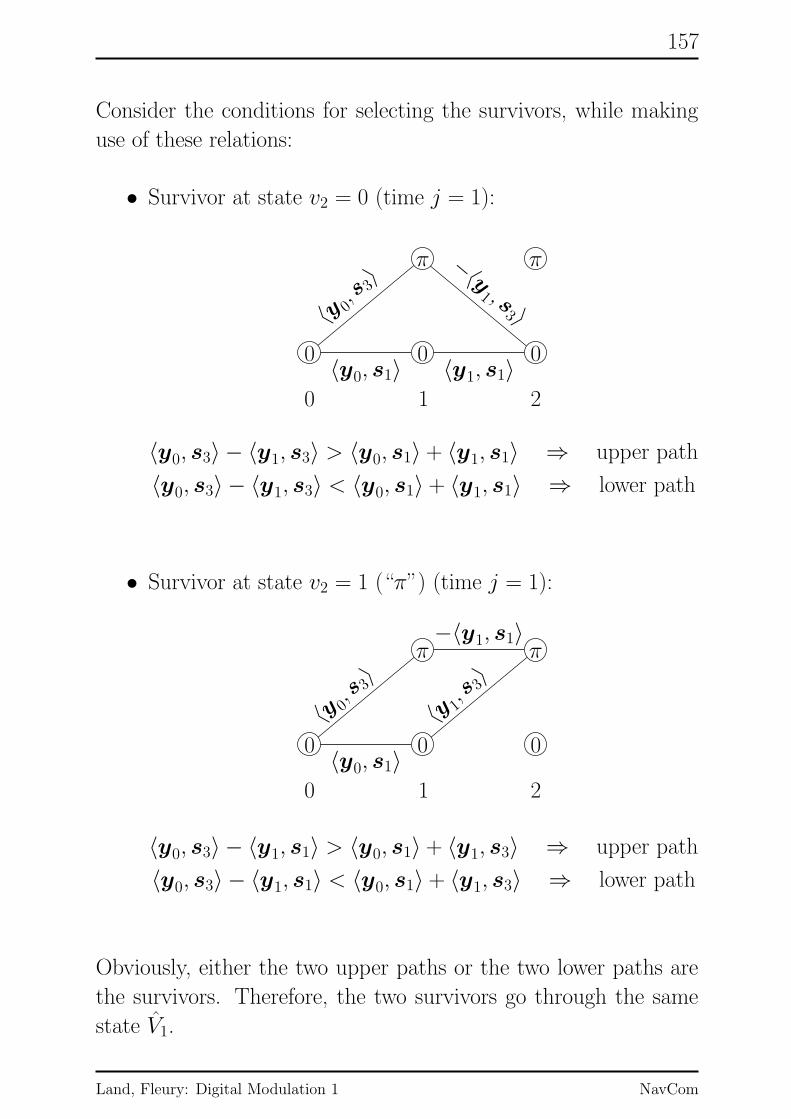
157
Consider the conditions for selecting the survivors, while making
use of these relations:
• Survivor at state v2 = 0 (time j = 1):
PSfrag replacements
00 0
π π
〈y0, s1〉
−〈y0, s1〉
〈y 0, s
3〉
−〈y0, s3〉
〈y1, s1〉
−〈y1, s1〉〈y1, s3〉
−〈y1 , s
3 〉
0 1 2
〈y0, s3〉 − 〈y1, s3〉 > 〈y0, s1〉 + 〈y1, s1〉 ⇒ upper path
〈y0, s3〉 − 〈y1, s3〉 < 〈y0, s1〉 + 〈y1, s1〉 ⇒ lower path
• Survivor at state v2 = 1 (“π”) (time j = 1):
PSfrag replacements
00 0
π π
〈y0, s1〉
−〈y0, s1〉
〈y 0, s
3〉
−〈y0, s3〉〈y1, s1〉
−〈y1, s1〉
〈y 1, s
3〉
−〈y1, s3〉
0 1 2
〈y0, s3〉 − 〈y1, s1〉 > 〈y0, s1〉 + 〈y1, s3〉 ⇒ upper path
〈y0, s3〉 − 〈y1, s1〉 < 〈y0, s1〉 + 〈y1, s3〉 ⇒ lower path
Obviously, either the two upper paths or the two lower paths are
the survivors. Therefore, the two survivors go through the same
state V1.
Land, Fleury: Digital Modulation 1 NavCom

158
ML State Sequence
By induction, we obtain the following optimal decision rule for
state Vj based on yj−1 and yj:
Vj =
{
0 if 〈yj−1, s3〉 − 〈yj, s3〉 < 〈yj−1, s1〉 + 〈yj, s1〉,1 if 〈yj−1, s3〉 − 〈yj, s3〉 > 〈yj−1, s1〉 + 〈yj, s1〉,
j = 1, 2, . . . , L− 1. (Remember: VL = 0 by convention.)
This decision rule can be simplified. The modulation symbols are
s1 = (+√
Es, 0)T, s3 = (0,+√
Es)T.
Thus, the inner products can be written as
〈yj, s1〉 = yj,1 ·√
Es, 〈yj, s3〉 = yj,2 ·√
Es.
Substituting this in the decision rule and dividing by√Es, we ob-
tain the following simplified (and still optimal) decision rule:
Vj =
{
0 if yj−1,2 − yj,2 < yj−1,1 + yj,1,
1 if yj−1,2 − yj,2 > yj−1,1 + yj,1,
j = 1, 2, . . . , L− 1.
Land, Fleury: Digital Modulation 1 NavCom

159
The following device implements this state decision rule:
PSfrag replacements
Yj−1,1Yj,1
Yj−1,2Yj,2
Zj,1
Zj,2
Zj Vj
T
T
zj > 0→ 0
zj < 0→ 1
Vector-Encoder Inverse
Given the sequence of state estimates {Vj}, the sequence of bit
estimates {Uj} can computed according to
Uj = Vj ⊕ Vj+1,
j = 0, 1, . . . , L− 1. (Compare vector encoder.)
The following device implements this operation:PSfrag replacements
Vj Vj−1 Uj−1
T
The time indices are j = 0, 1, . . . , L− 1, and VL = 0 as VL = 0 by
convention. Remember that UL−1 does not convey information.
Land, Fleury: Digital Modulation 1 NavCom
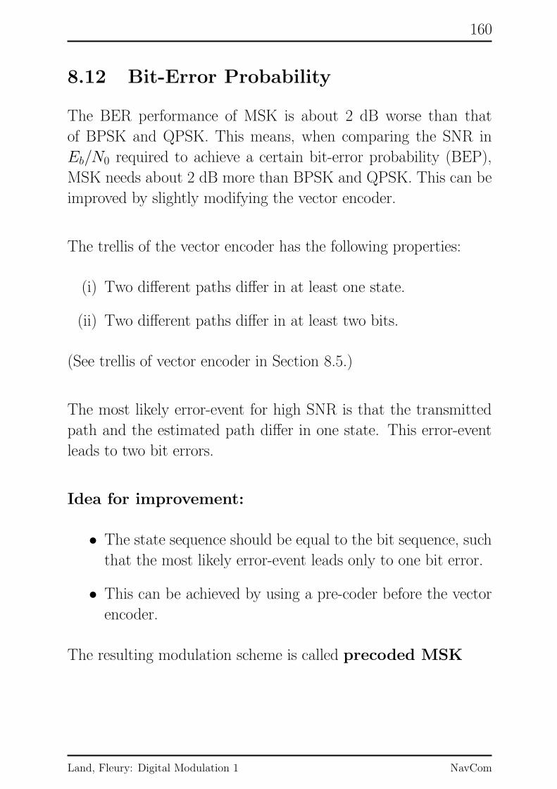
160
8.12 Bit-Error Probability
The BER performance of MSK is about 2 dB worse than that
of BPSK and QPSK. This means, when comparing the SNR in
Eb/N0 required to achieve a certain bit-error probability (BEP),
MSK needs about 2 dB more than BPSK and QPSK. This can be
improved by slightly modifying the vector encoder.
The trellis of the vector encoder has the following properties:
(i) Two different paths differ in at least one state.
(ii) Two different paths differ in at least two bits.
(See trellis of vector encoder in Section 8.5.)
The most likely error-event for high SNR is that the transmitted
path and the estimated path differ in one state. This error-event
leads to two bit errors.
Idea for improvement:
• The state sequence should be equal to the bit sequence, such
that the most likely error-event leads only to one bit error.
• This can be achieved by using a pre-coder before the vector
encoder.
The resulting modulation scheme is called precoded MSK
Land, Fleury: Digital Modulation 1 NavCom

161
8.13 Differential Encoding and DifferentialDecoding
The two terms “differential encoder” and “differential decoder”
are mainly used due to historical reasons. Both may be used as
encoders.
In the following, bj ∈ {0, 1} denote the bits before encoding, and
cj ∈ {0, 1} denote the bits after encoding.
Differential Encoder (DE)PSfrag replacements
bj cj+1 cjT
Operation:
cj+1 = bj ⊕ cj,j = 0, 1, 2, . . . . Initialization: c0 = 0.
Differential Decoder (DD)PSfrag replacements
bj bj−1 cjT
Operation:
cj = bj ⊕ bj−1,
j = 0, 1, 2, . . . . Initialization: b−1 = 0.
Land, Fleury: Digital Modulation 1 NavCom

162
8.14 Precoded MSK
The DD(!) is used as a pre-coder and is placed before the vector
encoder. The DE(!) is placed behind the vector-encoder inverse.
PSfrag replacements
Uj X(t)
W (t)
Y (t) Uj−1
DD MSK Tx MSK Rx / DE
Vector Representation of Precoded MSK
PSfrag replacements
Uj
U ′j
Vj = Uj−1
Xj,1
Xj,2T
s1
s2
s3
s4
00
01
10
11U ′jVj
Initialization: V0 = 0. Notice: U ′j = Uj ⊕ Vj = Uj ⊕ Uj−1.
PSfrag replacements
Yj−1,1Yj,1
Yj−1,2Yj,2
Zj,1
Zj,2
Zj Vj = Uj−1
T
T
zj > 0→ 0
zj < 0→ 1
Notice: The vector-encoder inverse and the DE compensate each
other and can be removed.
Land, Fleury: Digital Modulation 1 NavCom

163
Trellis of Precoded MSK
PSfrag replacements
000000
111111
0/s10/s10/s10/s1 0/s1
1/−s11/−s11/−s11/−s1
1/s 3
1/s 3
1/s 3
1/s 3
1/s 3
0/−s3
0/−s3
0/−s3
0/−s3
0 1 2 3 4 5
The thick path corresponds to the bit sequence
U [0,4] = [0, 1, 1, 0, 0].
Bit-Error Probability of Precoded MSK
The bit-error probability of precoded MSK is
Pb = Q(√
2γb),
γb = Eb/N0.
Sketch of the Proof:
The bit-error probability is given as
Pb = limL→∞
1
L
L−1∑
j=0
Pr(Uj 6= Uj).
All terms in this sum can shown to be identical, and thus
Pb = Pr(U0 6= U0).
Due to the precoding, we have U0 = V1, and therefore
Pb = Pr(V1 6= V1).
Land, Fleury: Digital Modulation 1 NavCom

164
This expression can be written using conditional probabilities:
Pb =
1∑
v=0
1∑
u=0
Pr(V1 6= V1|V1 = v, U1 = u) · Pr(V1 = v, U1 = u).
(Usual trick.) These conditional probabilities can shown to be all
identical, and thus
Pb = Pr(V1 6= V1|V1 = 0, U1 = 0).
As V1 = U0 (property of precoded MSK), we obtain
Pb = Pr(V1 = 1|U0 = 0, U1 = 0).
The ML decision rule is
V1 =
{
0 if y0,2 − y1,2 < y0,1 + y1,1,
1 if y0,2 − y1,2 > y0,1 + y1,1.
Given the hypothesis U0 = U1 = 0, we have
X0 = X1 = s1 = (√
Es, 0)T,
and so
Y0,1 =√
Es +W0,1, Y0,2 = W0,2,
Y1,1 =√
Es +W1,1, Y1,2 = W1,2.
Remember:
Y 0 = (Y0,1, Y0,2)T, Y 1 = (Y1,1, Y1,2)
T.
Land, Fleury: Digital Modulation 1 NavCom
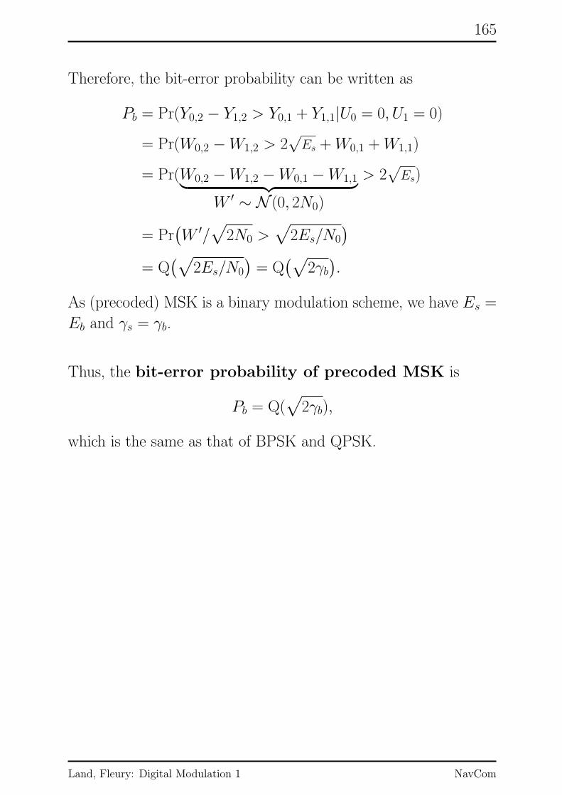
165
Therefore, the bit-error probability can be written as
Pb = Pr(Y0,2 − Y1,2 > Y0,1 + Y1,1|U0 = 0, U1 = 0)
= Pr(W0,2 −W1,2 > 2√
Es +W0,1 +W1,1)
= Pr(W0,2 −W1,2 −W0,1 −W1,1︸ ︷︷ ︸
W ′ ∼ N (0, 2N0)
> 2√
Es)
= Pr(W ′/
√
2N0 >√
2Es/N0
)
= Q(√
2Es/N0
)= Q
(√
2γb).
As (precoded) MSK is a binary modulation scheme, we have Es =
Eb and γs = γb.
Thus, the bit-error probability of precoded MSK is
Pb = Q(√
2γb),
which is the same as that of BPSK and QPSK.
Land, Fleury: Digital Modulation 1 NavCom
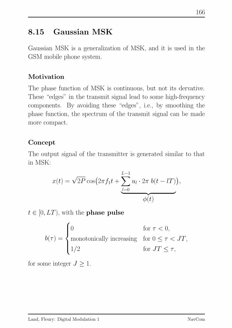
166
8.15 Gaussian MSK
Gaussian MSK is a generalization of MSK, and it is used in the
GSM mobile phone system.
Motivation
The phase function of MSK is continuous, but not its dervative.
These “edges” in the transmit signal lead to some high-frequency
components. By avoiding these “edges”, i.e., by smoothing the
phase function, the spectrum of the transmit signal can be made
more compact.
Concept
The output signal of the transmitter is generated similar to that
in MSK:
x(t) =√
2P cos(2πf1t +
L−1∑
l=0
ul · 2π b(t− lT )
︸ ︷︷ ︸
φ(t)
),
t ∈ [0, LT ), with the phase pulse
b(τ ) =
0 for τ < 0,
monotonically increasing for 0 ≤ τ < JT ,
1/2 for JT ≤ τ ,
for some integer J ≥ 1.
Land, Fleury: Digital Modulation 1 NavCom

167
Notice that there are two new degrees of freedom:
(i) The phase pulse may stretch over more than one symbol
duration T .
(ii) The phase pulse may be be selected such that its derivative
is zero for t = and t = JT .
Phase Pulse and Frequency Pulse
In GMSK, the phase pulse b(τ ) is constructed via its deriva-
tive c(τ ), called the frequency pulse:
(i) The frequency pulse c(τ ) is the convolution of a rectan-
gular pulse (as in MSK!) with a Gaussian pulse:
c(τ ) = rectangular pulse ∗ Gaussian pulse,
where c(τ ) = 0 for τ /∈ [0, JT ), and∫c(τ )dτ = 1/2. The
resulting pulse is
c(τ ) = Q( 2πB√
ln 2
(τ − T/2
)
− Q( 2πB√
ln 2
(τ + T/2
)).
The value B corresponds to a bandwidth and is a design
parameter.
(ii) The phase pulse is the integral over the frequency pulse:
b(τ ) =
τ∫
0
c(τ ′)dτ ′.
Due to the definition of the frequency pulse, we have b(τ ) =
1/2 for τ ≥ JT .
The resulting phase pulse fulfills the conditions given above.
Land, Fleury: Digital Modulation 1 NavCom

168
In GSM, the parameter B is chosen such that BT ≈ 0.3. The
length of the phase pulse is then L ≈ 4.
Land, Fleury: Digital Modulation 1 NavCom

169
9 Quadrature Amplitude Modula-tion
Land, Fleury: Digital Modulation 1 NavCom

170
10 BPAM with Bandlimited Wave-forms
Land, Fleury: Digital Modulation 1 NavCom

171
Part III
Appendix
Land, Fleury: Digital Modulation 1 NavCom

172
A Geometrical Representation ofSignals
A.1 Sets of Orthonormal Functions
The D real-valued functions
ψ1(t), ψ2(t), . . . , ψD(t)
form an orthonormal set if+∞∫
−∞
ψk(t)ψl(t) dt =
{
0 for k 6= l (orthogonality),
1 for k = l (normalization).
Example: D = 3
PSfrag replacements
t
t
t
ψ1(t)
ψ2(t)
ψ3(t)
T
T
T
1/√T
1/√T
1/√T
−1/√T
−1/√T
−1/√T
3
Land, Fleury: Digital Modulation 1 NavCom

173
A.2 Signal Space Spanned by an Orthonor-mal Set of Functions
Let{ψ1(t), ψ2(t), . . . , ψD(t)
}be a set of orthonormal functions.
We denote by Sψ the set containing all linear combinations of these
functions:
Sψ :={
s(t) : s(t) =
D∑
i=1
siψi(t); s1, s2, . . . , sD ∈ R
}
.
Example: (continued)
The following functions are elements of Sψ:
s1(t) = ψ1(t) + ψ2(t), s2(t) = 12ψ1(t)− ψ2(t) + 1
2ψ3(t)PSfrag replacements
t t
s1(t) s2(t)
T T
2/√T 2/
√T
−2/√T −2/
√T
3
The set Sψ is a vector space with respect to the following opera-
tions:
• Addition
+ :(s1(t), s2(t)
)7→ s1(t) + s2(t)
• Multiplication with a scalar
· :(a, s(t)
)7→ a · s(t)
Land, Fleury: Digital Modulation 1 NavCom

174
A.3 Vector Representation of Elements inthe Vector Space
With each element s(t) ∈ Sψ,
s(t) =
D∑
i=1
siψi(t),
we associate the D-dimensional real vector
s = [s1, s2, . . . , sD]T ∈ RD.
Example: (continued)
s1(t) = ψ1(t) + ψ2(t) 7→ s1 = [1, 1, 0]T ,
s2(t) = 12ψ1(t)− ψ2(t) + 1
2ψ3(t) 7→ s2 = [12,−1, 12]T .
3
Vectors in R, R2, R
3, can be represented geometrically by points
on the line, in the plane, an in the 3-dimensional Euclidean space,
respectively.
Example: (continued)
PSfrag replacements
ψ1
ψ2
ψ3
11
1
0.50.5
s1
s2
3
Land, Fleury: Digital Modulation 1 NavCom
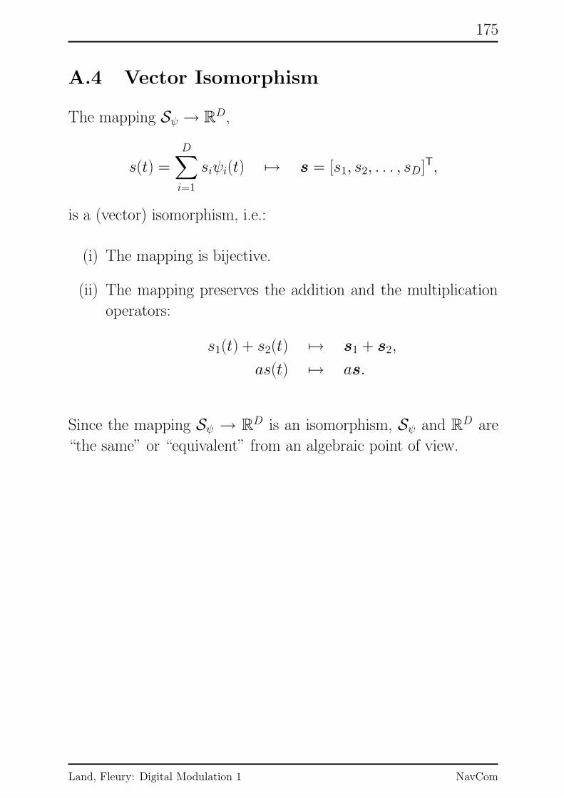
175
A.4 Vector Isomorphism
The mapping Sψ → RD,
s(t) =
D∑
i=1
siψi(t) 7→ s = [s1, s2, . . . , sD]T,
is a (vector) isomorphism, i.e.:
(i) The mapping is bijective.
(ii) The mapping preserves the addition and the multiplication
operators:
s1(t) + s2(t) 7→ s1 + s2,
as(t) 7→ as.
Since the mapping Sψ → RD is an isomorphism, Sψ and R
D are
“the same” or “equivalent” from an algebraic point of view.
Land, Fleury: Digital Modulation 1 NavCom

176
A.5 Scalar Product and Isometry
Scalar product in Sψ:
〈s1(t), s2(t)〉 :=
+∞∫
−∞
s1(t)s2(t) dt
for s1(t), s2(t) ∈ Sψ.
Scalar product in RD:
〈s1, s2〉 :=
D∑
i=1
s1,is2,i
for s1, s2 ∈ RD.
Relation of scalar products:
Each element in Sψ is a linear combination of
ψ1(t), ψ2(t), . . . , ψD(t):
s1(t) =
D∑
k=1
s1,kψk(t), s2(t) =
D∑
l=1
s2,lψl(t).
Inserting the two sums into the definition of the scalar product, we
obtain
〈s1(t), s2(t)〉 =
∫ ( D∑
k=1
s1,kψk(t))( D∑
l=1
s2,lψl(t))
dt =
=
D∑
k=1
D∑
l=1
s1,ks2,l
∫
ψk(t)ψl(t)dt︸ ︷︷ ︸
“orthonormality”
=
D∑
k=1
s1,ks2,k = 〈s1, s2〉
Hence the mapping Sψ → RD preserves the scalar product, i.e., it
is an isometry.
Land, Fleury: Digital Modulation 1 NavCom

177
Norms in Sψ
‖s(t)‖2 := 〈s(t), s(t)〉 =
∫
s2(t) dt = Es
The value Es is the energy of s(t).
Norms in RD:
‖s‖2 := 〈s, s〉 =
D∑
i=1
s2i
From the isometry and the definitions of the norms, we obtain the
Parseval relation
‖s(t)‖2 = ‖s‖2.
Land, Fleury: Digital Modulation 1 NavCom

178
A.6 Waveform Synthesis
Let{ψ1(t), ψ2(t), . . . , ψD(t)
}be a set of orthonormal functions
spanning the vector space Sψ. Every element s(t) ∈ Sψ can be
synthesized from its vector representation s = [s1, s2, . . . , sD]T by
one of the following devices.
Multiplicative-based Synthesizer
PSfrag replacements
s
s1
s2
sD
ψ1(t)
ψ2(t)
ψD(t)
δ(t)
s(t) =
D∑
k=1
skψk(t)
Filter-bank based Synthesizer
Filter
Filter
Filter
PSfrag replacements
ss1
s2
sD
ψ1(t)
ψ2(t)
ψD(t)
δ(t)
s(t)
s(t) =
D∑
k=1
skδ(t) ∗ ψk(t) with Dirac function δ(t)
Land, Fleury: Digital Modulation 1 NavCom

179
A.7 Implementation of the Scalar Product
Let s1(t) and s2(t) be time-limited to the interval [0, T ]. Then
〈s1(t), s2(t)〉 :=
T∫
0
s1(t)s2(t) dt.
The scalar product can be computed by the following two devices.
Correlator-based ImplementationPSfrag replacements
s1(t)
s2(t)
∫ T
0 (.)dt 〈s1(t), s2(t)〉
Matched-filter based Implementation
We seek a linear filter that outputs the value 〈s1(t), s2(t)〉 at a
certain time, say t0.
PSfrag replacements
s1(t) g(t)linear filter
sample attime t0
〈s1(t), s2(t)〉
We want
〈s1(t), s2(t)〉 =
T∫
0
s1(τ )s2(τ ) dτ!=
+∞∫
−∞
s1(τ )g(t′ − τ ) dτ∣∣∣t′=t0
The second equality holds for
s2(τ ) = g(t0 − τ ) ⇔ g(t) = s2(t0 − t)
Land, Fleury: Digital Modulation 1 NavCom

180
Example:
PSfrag replacements
tt
t0
s2(t) s2(t0 − t)
TT
3
The filter is causal and thus realizable for a function time-limited
to the interval [0, T ] if
t0 ≥ T.
The value t0 is the time at which the value 〈s1(t), s2(t)〉 appears
at the filter output. Choosing the minimum value, i.e., t0 = T , we
obtain the following (realizable) implementation.
PSfrag replacements
s1(t) s2(T − t)matched filter
sample attime T
〈s1(t), s2(t)〉
The filter is matched to s2(t).
Land, Fleury: Digital Modulation 1 NavCom

181
A.8 Computation of the Vector Represen-tation
Let{ψ1(t), ψ2(t), . . . , ψD(t)
}be a set of orthonormal functions
time-limited to [0, T ] and spanning the vector space Sψ.
We seek a device that computes the vector representation s ∈ RD
for any function s(t) ∈ Sψ, i.e.,
s = [s1, s2, . . . , sD]T such that s(t) =
D∑
k=1
skψk(t).
The components of s can be computed as
sk = 〈s(t), ψk(t)〉, k = 1, 2, . . . , D.
Correlator-based ImplementationPSfrag replacements
s(t) ψ1(t)
ψD(t)
∫ T
0 (.)dt
∫ T
0 (.)dt
s1
sD
Matched-filter based Implementation
PSfrag replacements
s(t)
ψ1(T − t)
ψD(T − t)MF
MF s1
sDsample attime T
Land, Fleury: Digital Modulation 1 NavCom

182
A.9 Gram-Schmidt Orthonormalization
Assume a set of M signal waveforms{
s1(t), s2(t), . . . , sM(t)}
spanning a D-dimensional vector space. From these waveforms,
we can construct a set of D ≤M orthonormal waveforms{
ψ1(t), ψ2(t), . . . , ψD(t)}
by applying the following procedure.
Remember:
〈s1(t), s2(t)〉 =
∫
s1(t)s2(t) dt
‖s(t)‖2 := 〈s(t), s(t)〉 = Es
Gram-Schmidt orthonormalization procedure
1. Take the first waveform s1(t) and normalize it to unit energy:
ψ1(t) :=s1(t)
√
‖s1(t)‖2.
2. Take the second waveform s2(t). Determine the projection
of s2(t) onto ψ1(t), and subtract this projection from s2(t):
c2,1 = 〈s2(t), ψ1(t)〉,s′2(t) = s2(t)− c2,1ψ1(t).
Normalize s′2(t) to unit energy:
ψ2(t) :=s′2(t)
√
‖s′2(t)‖2.
Land, Fleury: Digital Modulation 1 NavCom

183
3. Take the third waveform s3(t). Determine the projections
of s3(t) onto ψ1(t) and onto ψ2(t), and subtract these pro-
jections from s3(t):
c3,1 = 〈s3(t), ψ1(t)〉,c3,2 = 〈s3(t), ψ2(t)〉,s′3(t) = s3(t)− c3,1ψ1(t)− c3,2ψ2(t).
Normalize s′3(t) to unit energy:
ψ3(t) :=s′3(t)
√
‖s′3(t)‖2.
4. Proceed in this way for all other waveforms sk(t) until k = D.
Notice that s′k(t) = 0 for k > D. (Why?)
The general rule is the following. For k = 1, 2, . . . , D,
ck,i = 〈sk(t), ψi(t)〉, i = 1, 2, . . . , k − 1
s′k(t) = sk(t)−k−1∑
i=1
ck,iψi(t),
ψk(t) :=s′k(t)
√‖s′k(t)‖2
.
Due to this procedure, the resulting waveforms ψk(t) are orthog-
onal and normalized, as desired, and they form an orthonormal
basis of the D-dimensional vector space of the waveforms si(t).
Remark: The set of orthonormal waveforms is not unique.
Land, Fleury: Digital Modulation 1 NavCom

184
Example: Orthonormalization
Original signal waveforms:
PSfrag replacements
t
tt
t
s1(t)
s2(t)
s3(t)
s4(t)
0
00
0
1
1 1
1
1
1
1
1
2 2
22
3
33
3−1
−1−1
−11/√
2
−1/√
2
Set 1 of orthonormal waveforms:
PSfrag replacements
t
t
t
ψ1(t)
ψ2(t)
ψ3(t)
0
0
0
1
1
1
1
2
2
2
3
3
3
−1
1/√
2
1/√
2
−1/√
2
−1/√
2
Set 2 of orthonormal waveforms:
PSfrag replacements
t
t
t
ψ1(t)
ψ2(t)
ψ3(t)
0
0
0
1
1
1
1
1
1
2
2
2
3
3
3
−1
−1
−11/√
2
−1/√
23
Land, Fleury: Digital Modulation 1 NavCom

185
B Orthogonal Transformation of aWhite Gaussian Noise Vector
The statistical properties of a white Gaussian noise vector
(WGNV) are invariant with respect to orthonormal transforma-
tions. This is first shown for a vector with two dimensions, and
then for a vector with an arbitrary number of dimensions.
B.1 The Two-Dimensional Case
Let W denote a 2-dimensional WGNV, i.e.,
W =
[W1
W2
]
∼ N([
0
0
]
,
[σ2 0
0 σ2
])
.
Consider the original coordinate system (ξ1, ξ2) and the rotated
coordinate system (ξ ′1, ξ′2).
PSfrag replacements
ξ1
ξ2
ξ′1
ξ′2
α = π/4
w
w1
w2
w′1
w′2
Let [W ′1,W
′2]
T denote the components of W expressed with respect
to the rotated coordinate system (ξ ′1, ξ′2):
W ′1 = +W1 cosα +W2 sinα
W ′2 = −W1 sinα +W2 cosα.
Land, Fleury: Digital Modulation 1 NavCom

186
Writing this in matrix notation as[W ′
1
W ′2
]
=
[cosα sinα
− sinα cosα
] [W1
W2
]
,
the vector W ′ can seen to be the orthonormal transformation of
the vector W .
The resulting vector W ′ = [W ′1,W
′2]
T is also a two-dimensional
WGNV with the same covariance matrix as W = [W1,W2]T:
W ′ =
[W ′
1
W ′2
]
∼ N([
0
0
]
,
[σ2 0
0 σ2
])
.
Proof: See problem.
B.2 The General Case
Let W = [W1, . . . ,WD]T denote a D-dimensional WGNV with
zero mean and covariance matrix σ2I , i.e.,
W ∼ N(0, σ2I
).
(0 is a column vector of length D, and I is the D × D identity
matrix.) Let further V denote an orthonormal transformation
RD → R
D, i.e., a linear transformation with the property
V V T = V TV = I.
Then the transformed vector
W ′ = V W
is also a D-dimensional WGNV with the same covariance matrix
as W :
W ′ ∼ N(0, σ2I
).
Land, Fleury: Digital Modulation 1 NavCom

187
Proof
(i) A linear transformation of a Gaussian random vector is again
a Gaussian random vector; thus W ′ is Gaussian.
(ii) The mean value is
E[W ′] = E
[V W
]= V E
[W]
= 0.
(iii) The covariance matrix is
E[W ′W ′T] = E
[V WW TV T
]
= V E[WW T
]
︸ ︷︷ ︸
σ2I
V T = σ2 V V T︸ ︷︷ ︸
I
= σ2I.
Comment
In the case D = 2, V takes the form
V =
[cosα sinα
− sinα cosα
]
for some α ∈ [0, 2π).
Land, Fleury: Digital Modulation 1 NavCom

188
C The Shannon Limit
C.1 Capacity of the Band-limited AWGNChannel
Consider an AWGN channel with bandwidth W [1/sec]. The ca-
pacity of this channel is given by
CW = W log2
(1 +
S
WN0
)[bit/sec].
Consider further a digital transmission scheme operating at trans-
mission rate R [bit/sec] with limited transmit power S.
Channel Coding Theorem (C.E. Shannon, 1948):
Consider a binary random sequence generated by a BSS
that is transmitted over an AWGN channel with band-
width W using some transmission scheme.
Transmission with an arbitrarily small probability of er-
ror (using an appropriate coding/modulation scheme)
is possible provided that the transmission rate is less
than the channel capacity, i.e.,
Pb → 0 is possible if R < CW .
Conversely, error-free transmission is impossible if the
rate is larger than the channel capacity, i.e.,
Pb → 0 is impossible if R > CW .
Land, Fleury: Digital Modulation 1 NavCom

189
A coding/modulation scheme can be characterized by its spectral
efficiency and its power efficiency. The spectral efficiency is
the ratio R/W , and it has the unit bitsec Hz. The power efficiency
is the SNR γb = Eb/N0 necessary to achieve a certain error prob-
ability (e.g., 10−5).
Example: MPAM
The rate is given by R = 1T log2M . The bandwidth required to
transmit pulses of duration T is about W = 1/T . The spectral
efficiency is thus
R
W= log2M
bit
sec Hz.
Error probabilities can be found in [1, p. 412, 435]. 3
Example: MPPM
The rate is given by R = 1T log2M . The bandwidth required
to transmit pulses of duration T/M is about W = M/T . The
spectral efficiency is thus
R
W=
log2M
M
bit
sec Hz.
Error probabilities can be found in [1, p. 426, 435]. 3
Land, Fleury: Digital Modulation 1 NavCom
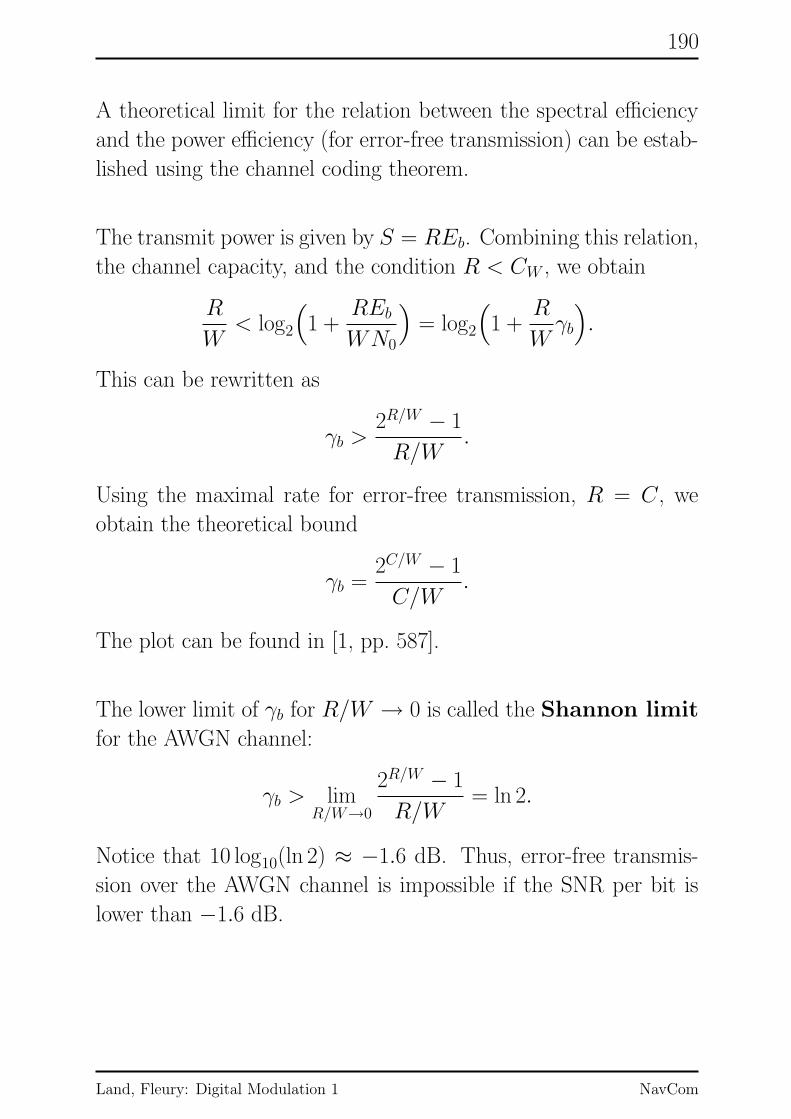
190
A theoretical limit for the relation between the spectral efficiency
and the power efficiency (for error-free transmission) can be estab-
lished using the channel coding theorem.
The transmit power is given by S = REb. Combining this relation,
the channel capacity, and the condition R < CW , we obtain
R
W< log2
(
1 +REb
WN0
)
= log2
(
1 +R
Wγb
)
.
This can be rewritten as
γb >2R/W − 1
R/W.
Using the maximal rate for error-free transmission, R = C, we
obtain the theoretical bound
γb =2C/W − 1
C/W.
The plot can be found in [1, pp. 587].
The lower limit of γb for R/W → 0 is called the Shannon limit
for the AWGN channel:
γb > limR/W→0
2R/W − 1
R/W= ln 2.
Notice that 10 log10(ln 2) ≈ −1.6 dB. Thus, error-free transmis-
sion over the AWGN channel is impossible if the SNR per bit is
lower than −1.6 dB.
Land, Fleury: Digital Modulation 1 NavCom

191
C.2 Capacity of the Band-UnlimitedAWGN Channel
For the AWGN channel with unlimited bandwidth (but still
limited transmit power), the capacity is given by
C∞ = limW→∞
W log2
(
1 +S
WN0
)
=1
ln 2
S
N0.
The conditionR < C∞ becomes then equivalent with the condition
γb > ln 2. (Remember: S = REb.)
Land, Fleury: Digital Modulation 1 NavCom