A Model for Analyzing Heating and Cooling Demand for Atria ...

Brigham Young University Brigham Young University

BYU ScholarsArchive BYU ScholarsArchive

Theses and Dissertations

2014-07-08

A Model for Analyzing Heating and Cooling Demand for Atria A Model for Analyzing Heating and Cooling Demand for Atria

Between Tall Buildings Between Tall Buildings

Samuel David Christensen Brigham Young University - Provo

Follow this and additional works at: https://scholarsarchive.byu.edu/etd

Part of the Civil and Environmental Engineering Commons

BYU ScholarsArchive Citation BYU ScholarsArchive Citation Christensen, Samuel David, "A Model for Analyzing Heating and Cooling Demand for Atria Between Tall Buildings" (2014). Theses and Dissertations. 4211. https://scholarsarchive.byu.edu/etd/4211

This Thesis is brought to you for free and open access by BYU ScholarsArchive. It has been accepted for inclusion in Theses and Dissertations by an authorized administrator of BYU ScholarsArchive. For more information, please contact [email protected], [email protected].

http://home.byu.edu/home/

http://home.byu.edu/home/

https://scholarsarchive.byu.edu/

https://scholarsarchive.byu.edu/etd

https://scholarsarchive.byu.edu/etd?utm_source=scholarsarchive.byu.edu%2Fetd%2F4211&utm_medium=PDF&utm_campaign=PDFCoverPages

http://network.bepress.com/hgg/discipline/251?utm_source=scholarsarchive.byu.edu%2Fetd%2F4211&utm_medium=PDF&utm_campaign=PDFCoverPages

https://scholarsarchive.byu.edu/etd/4211?utm_source=scholarsarchive.byu.edu%2Fetd%2F4211&utm_medium=PDF&utm_campaign=PDFCoverPages

mailto:[email protected],%[email protected]

i

A Model for Analyzing Heating and Cooling Demand

for Atria Between Tall Buildings

Samuel David Christensen

A thesis submitted to the faculty of Brigham Young University

in partial fulfillment of the requirements for the degree of

Master of Science

Richard J. Balling, Chair Matthew R. Jones Grant G. Schultz

Department of Civil and Environmental Engineering

Brigham Young University

July 2014

Copyright © 2014 Samuel David Christensen

All Rights Reserved

ii

ABSTRACT

A Model for Analyzing Heating and Cooling Demand for Atria Between Tall Buildings

Samuel David Christensen

Department of Civil and Environmental Engineering, BYU Master of Science

The heating and air-conditioning energy demand of skyscrapers with atria between

buildings is explored. Radiation, conduction, convection, and ventilation were evaluated to determine annual heating and cooling energy demands for a 100-building city located in Provo, Utah. Spreadsheets models were developed and calibrated with a computational fluid dynamics model. Three spreadsheet model cases were examined: a baseline no-atrium case, a conditioned atrium case, and an unconditioned atrium case. The energy demands and atrium temperatures were compared between the different cases. The research concludes that atria can be used between buildings to reduce the heating and cooling energy demands. The exposed surface area of the city was reduced by 73.7%. This resulted in a 49.7% reduction in heating and cooling energy consumption for the unconditioned atrium case and a 16.0% reduction in energy consumption for the conditioned atrium case.

Keywords: Greenplex, atrium, energy, heating, air-conditioning

iii

ACKNOWLEDGEMENTS

I wish to acknowledge my advisor Dr. Richard J. Balling for his patience and greenplex

vision. Dr. Matthew R. Jones was invaluable in teaching me heat transfer and helping me

develop the tools necessary to complete this project. I wish to thank Dr. Schultz for his lessons

on consistency and attention to detail. I would also like to thank the Fulton Super Computing

Lab for their assistance with coding and running my CFD models.

I am particularly grateful to my wonderful wife for supporting me through graduate

school and proof-reading this thesis. I would like to thank my parents and my in-laws who taught

me the value of hard work and knowledge. This project would not have been possible without

their support and encouragement.

I would like to thank Ryan Bessey for his technical resources on ETFE, Dr. Steven

Gorrel, Dr. Scott Thompson, and Sampat Nidadavolu for answering my CFD questions and

helping me troubleshoot my models. I would also like to thank King Hussein for funding this

research.

iv

TABLE OF CONTENTS

1 Introduction ........................................................................................................................... 1

2 Literature Review ................................................................................................................. 4

2.1 Atria History ................................................................................................................... 4

2.2 Modern Atria Characteristics .......................................................................................... 5

2.3 Atrium Issues and Solutions ........................................................................................... 7

2.4 Atrium Simulation ........................................................................................................ 10

2.5 Chapter Summary ......................................................................................................... 15

3 Conditioned Atrium Spreadsheet Model .......................................................................... 16

3.1 Problem Definition ....................................................................................................... 16

3.2 Spreadsheet Description ............................................................................................... 18

3.2.1 Constants Sheet ......................................................................................................... 18

3.2.2 Monthly Sheets ......................................................................................................... 23

3.2.3 Annual Sheet ............................................................................................................. 31

3.2.4 Reference Sheet......................................................................................................... 32

3.3 Chapter Summary ......................................................................................................... 34

4 No-Atrium Spreadsheet Model .......................................................................................... 35

v


4.2 Chapter Summary ......................................................................................................... 36

5 Unconditioned Atrium Spreadsheet Model ...................................................................... 38


5.2 Development ................................................................................................................. 41

5.3 Chapter Summary ......................................................................................................... 42

6 Calibration of Spreadsheet Models with CFD ................................................................. 43

6.1 CFD Model Definition and Assumptions ..................................................................... 43

6.2 Procedure ...................................................................................................................... 44

6.3 CFD Model Results ...................................................................................................... 47

6.4 Limitations .................................................................................................................... 50

6.5 Comparison with Spreadsheet and Hand Calculated Results ....................................... 52

6.6 Chapter Summary ......................................................................................................... 54

7 Results and Discussion ........................................................................................................ 55

7.1 Energy Demand ............................................................................................................ 55

7.2 Temperature Ranges ..................................................................................................... 57

7.3 Discussion of Results .................................................................................................... 58

vi

7.4 Assumptions and Limitations ....................................................................................... 59

7.5 Future Research ............................................................................................................ 61

7.6 Chapter Summary ......................................................................................................... 64

8 Conclusions .......................................................................................................................... 65

vii

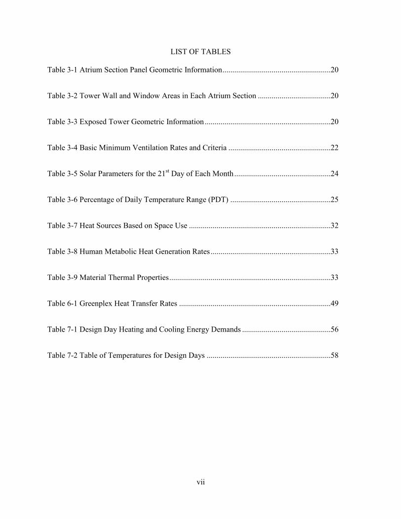
LIST OF TABLES

Table 3-1 Atrium Section Panel Geometric Information .......................................................20

Table 3-2 Tower Wall and Window Areas in Each Atrium Section .....................................20

Table 3-3 Exposed Tower Geometric Information ................................................................20

Table 3-4 Basic Minimum Ventilation Rates and Criteria ....................................................22

Table 3-5 Solar Parameters for the 21st Day of Each Month .................................................24

Table 3-6 Percentage of Daily Temperature Range (PDT) ...................................................25

Table 3-7 Heat Sources Based on Space Use ........................................................................32

Table 3-8 Human Metabolic Heat Generation Rates .............................................................33

Table 3-9 Material Thermal Properties ..................................................................................33

Table 6-1 Greenplex Heat Transfer Rates .............................................................................49

Table 7-1 Design Day Heating and Cooling Energy Demands .............................................56

Table 7-2 Table of Temperatures for Design Days ...............................................................58

viii

LIST OF FIGURES

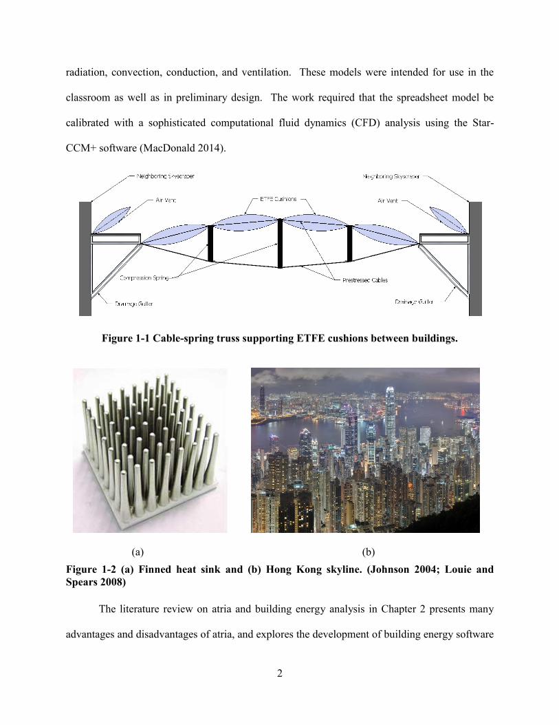
Figure 1-1 Cable-spring truss supporting ETFE cushions between buildings. ......................2

Figure 1-2 (a) Finned heat sink and (b) Hong Kong skyline. ................................................2

Figure 2-1 Atrium in Halifax Town Hall, UK built in 1863 ..................................................5

Figure 2-2 Parkview Green atrium with ETFE roof and glass walls .....................................6

Figure 2-3 Variable shading ETFE foils used in the Kingsdale School in London, UK .......8

Figure 2-4 Hydronic cooling fins under balconies in the Parkview Green atrium ................9

Figure 3-1 Pyramid greenplex ...............................................................................................17

Figure 3-2 Comparison of several different convection correlations. ...................................21

Figure 3-3 Solar geometry angles. .........................................................................................25

Figure 5-1 Basic resistor model .............................................................................................41

Figure 6-1 Volume mesh on a horizontal cross section through the city...............................45

Figure 6-2 Plots of heat transfer rate for the city for different base size values. ...................48

Figure 6-3 Heat transfer rates for the greenplex vs. wind speed at 5 meter base size. ..........48

Figure 6-4 Heat transfer rates through the walls from a 2.0m/s wind. ..................................49

Figure 6-5 Horizontal flow vector plane showing flow around buildings. ............................50

Figure 6-6 Total greenplex heat transfer rate for a temperature difference of 65°F ..............53

ix

Figure 6-7 Convection resistance values (R-Values) for different convection ......................54

Figure 7-1 Plot of the Design Day energy demand for the different atria cases ....................56

Figure 7-2 Plot of the high and low air temperatures. ...........................................................57

1

1 INTRODUCTION

The research described in this thesis investigated the heating, ventilation, air conditioning

(HVAC) energy demand of a new urban form called the “greenplex”. The greenplex is defined

as a car-free city composed of tall buildings interconnected with sky bridges and atria between

the buildings. Such atria may be constructed by spanning between the roofs of the buildings with

a network of cable-spring trusses supporting cushions made from the transparent material

Ethylene TetraFluoroEthylene (ETFE) as shown in Figure 1-1. These atria protect people from

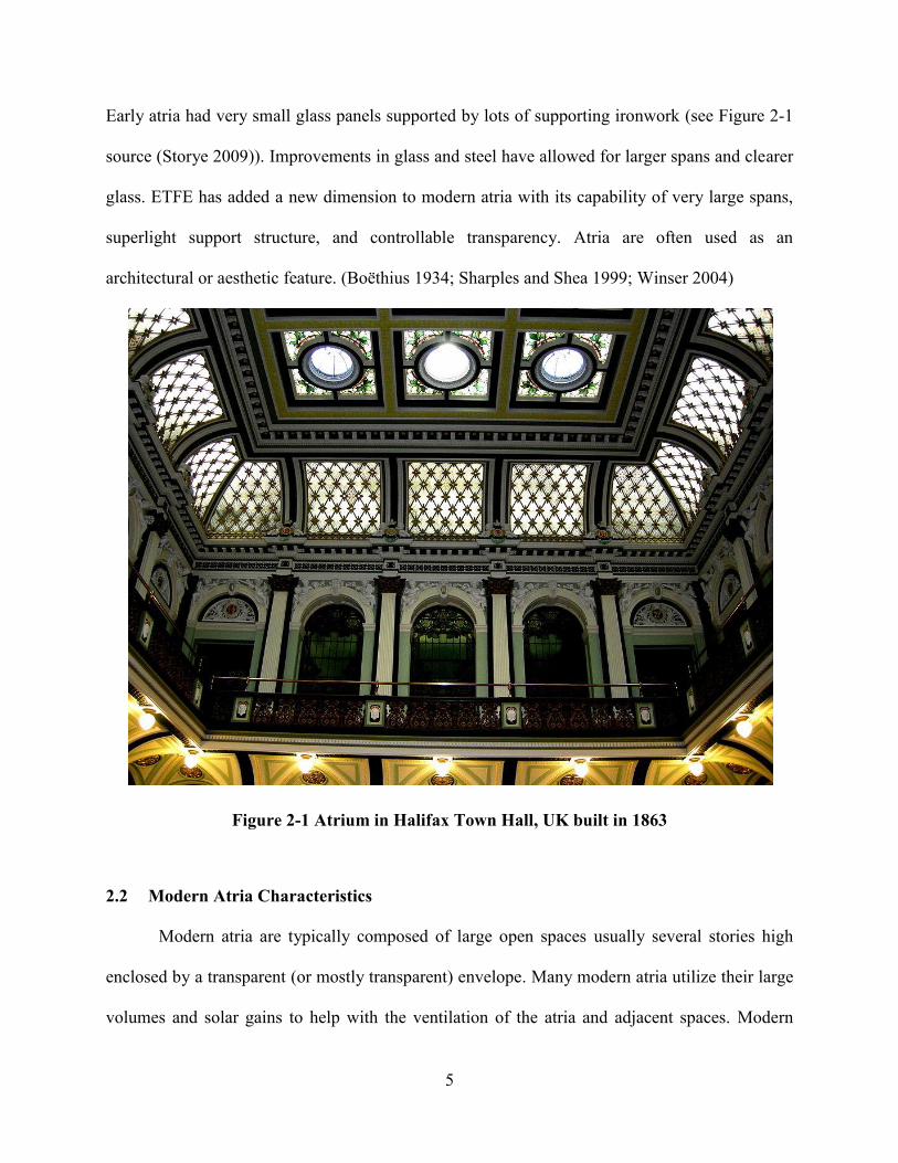
severe weather conditions. The tall fins on the thermal heat sink in Figure 1-2 (a) are designed to

maximize heat transfer. Tall buildings like those shown in Figure 1-2 (b) also transfer a lot of

energy to and from the surrounding environment. An additional benefit of the ETFE atria is that

the exposed surface area of the greenplex system is far less than that of buildings without atria,

potentially leading to significant reductions in HVAC energy demand.

The contributions of this work were: 1) to determine how much the HVAC energy

demand could be reduced by placing atria between tall buildings and 2) to develop spreadsheet

models capable of determining annual heating and cooling demands in buildings with atria. To

determine how much HVAC energy demand could be reduced by placing atria between tall

buildings, three cases (a no-atrium case, conditioned atrium case, and unconditioned atrium case)

were defined and analyzed. Three spreadsheet models were developed to evaluate these cases.

The spreadsheet models needed to adequately model atria and account for internal heat gains,

2

radiation, convection, conduction, and ventilation. These models were intended for use in the

classroom as well as in preliminary design. The work required that the spreadsheet model be

calibrated with a sophisticated computational fluid dynamics (CFD) analysis using the Star-

CCM+ software (MacDonald 2014).

Figure 1-1 Cable-spring truss supporting ETFE cushions between buildings.

(a) (b) Figure 1-2 (a) Finned heat sink and (b) Hong Kong skyline. (Johnson 2004; Louie and Spears 2008)

The literature review on atria and building energy analysis in Chapter 2 presents many

advantages and disadvantages of atria, and explores the development of building energy software

3

and models. This work presents the spreadsheet models for the conditioned atrium case in

Chapter 3, the no atrium case in Chapter 4, and the unconditioned atrium case in Chapter 5.

Calibration of the spreadsheet models using CFD analysis is presented in Chapter 6. The

research results from the spreadsheet models are presented and discussed in Chapter 7 along with

ideas for future research. Conclusions on the analyses and research are presented in Chapter 8.

4

2 LITERATURE REVIEW

Buildings in the United States collectively use a large portion of the nation's total energy

consumption to maintain a comfortable indoor environment. There are two approaches to saving

energy according to Tam (2011): increasing efficiency and decreasing demand. Many incentives

including Leadership in Energy and Environmental Design (LEED) certification and tax breaks

have been employed to get owners and developers to increase the energy efficiency of current

and future buildings within reasonable fiscal and comfort limits (USGBC 2009). Reducing

energy demands has been the driving force behind the establishment of the Department of

Energy and HVAC engineering procedures and analysis models for the last century and

especially since the 1973 oil embargo (Hunn et al. 2010). Good HVAC design and management

result in a comfortable indoor environment for people at a minimized cost to maintain. This

literature review explores atria history, characteristics, issues and solutions, and HVAC

simulation.

2.1 Atria History

The atria's beginnings can be traced back to the courtyards and central halls of the Greek

and Roman eras. They were employed to allow light and ventilation into inner rooms of

buildings. Glazed atria did not exist until the mid 19th century when glass and iron technological

advancements made spanning larger distances with a brittle glass more feasible. Glazing causes a

reduction in natural light penetration in exchange for protection from the outside environment.

5

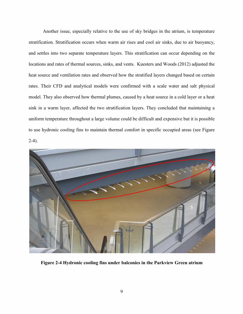
Early atria had very small glass panels supported by lots of supporting ironwork (see Figure 2-1

source (Storye 2009)). Improvements in glass and steel have allowed for larger spans and clearer

glass. ETFE has added a new dimension to modern atria with its capability of very large spans,

superlight support structure, and controllable transparency. Atria are often used as an

architectural or aesthetic feature. (Boëthius 1934; Sharples and Shea 1999; Winser 2004)

Figure 2-1 Atrium in Halifax Town Hall, UK built in 1863

2.2 Modern Atria Characteristics

Modern atria are typically composed of large open spaces usually several stories high

enclosed by a transparent (or mostly transparent) envelope. Many modern atria utilize their large

volumes and solar gains to help with the ventilation of the atria and adjacent spaces. Modern

6

atria utilize more insulative and clear fenestration and are capable of spanning very large

distances (see Figure 2-2). Even though the primary function of many atria is aesthetics, many

atria are also used to help with the building's natural or mixed-mode ventilation strategy.

Figure 2-2 Parkview Green atrium with ETFE roof and glass walls

Atria are becoming more popular in architectural applications according to Hung and

Chow (2001) because of their versatility and architectural beauty. In highly populated areas like

Hong Kong, atria are being used more often as public spaces because they are large and light

enough to feel like outside but often more comfortable (Xue et al. 2012). This increased

popularity has exposed many issues with atrium design.

7

2.3 Atrium Issues and Solutions

Atria have several issues that typically govern how they are designed. One issue is light

penetration into the adjacent rooms and areas. There are also conditioning issues with solar gains

in large, highly glazed areas like atria as well as temperature stratification issues. Finally, atrium

envelopes are somewhat limited in their insulation capability. Each of these issues poses a

problem to the aesthetics and/or cost of the atrium, and some of them compete with each other.

Atria are often used to bring natural light into areas of a building that otherwise could

only be artificially lit. This can help reduce the cost of artificial lighting. The first issue with

using an atrium to provide natural light is that the envelope blocks some of the sunlight. Sharples

and Shea (1999) conducted a study on atrium roof configurations under real sky conditions. They

concluded that mathematical models used did not accurately account for the loss of light

penetration due to the envelope. This implies that the envelope needs to be considered when

analyzing natural lighting. Once the natural lighting in the atrium is accounted for, the next issue

is with the amount that gets into the adjacent rooms. Du and Sharples (2011) explored how far

natural light gets into areas directly adjacent to a rectangular atria. They used a ray-tracing

program with a parametric model to adjust the atrium size, building height, room depths, balcony

proportions, and wall reflectivity. They found that more light penetrates deeper in the upper story

rooms and less light penetrates shallower in the lower story rooms. However, if adjacent room

walls and windows are designed well, the differences in natural light penetration between the top

floors and the bottom or middle floors can be minimized. This implies that there is a tradeoff

between less expensive construction and uniform natural lighting for the areas near the bottom of

the atrium.

8

Atrium envelopes require regular maintenance and cleaning. Even with self-cleaning

glass or ETFE, dust and debris accumulate over time on the surfaces of the envelope. This debris

affects the amount of natural light that gets into the atrium and the atrium's aesthetic appeal.

Cleaning cost must be added to the atrium design. (Gritch and Eason 2010)

Natural lighting is great for aesthetics but can increase solar gains. During the winter

months solar gains are a welcome source of free heating, but during the summer months solar

gains become an extra load on the air-conditioning system and might result in very

uncomfortable conditions in the atrium. (Chwieduk 2009) One technology that has been

developed to help control solar gains is variable shading ETFE foil cushions (see Figure 2-3).

These cushions consist of two layers with positive and negative printed patterns that transmit

sunlight when the layers are apart and reflect sunlight when the layers are together. (Colmenar-

Santos et al. 2013; Vector Foiltec 2012) Another solution for glass envelopes is shading through

the use of blinds, panels, or even photovoltaic panels. (James et al. 2009)

Figure 2-3 Variable shading ETFE foils used in the Kingsdale School in London, UK and Festo headquarters in Esslingen, Germany. (Vector Foiltec 2012)

9

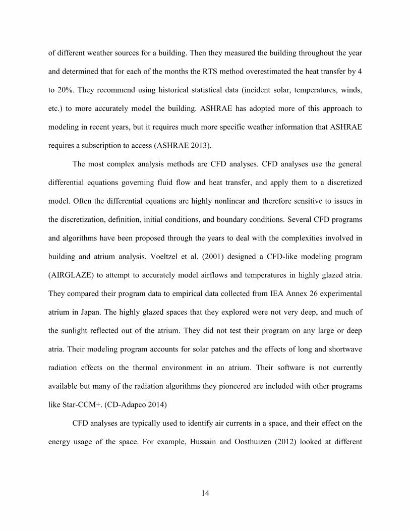
Another issue, especially relative to the use of sky bridges in the atrium, is temperature

stratification. Stratification occurs when warm air rises and cool air sinks, due to air buoyancy,

and settles into two separate temperature layers. This stratification can occur depending on the

locations and rates of thermal sources, sinks, and vents. Kuesters and Woods (2012) adjusted the

heat source and ventilation rates and observed how the stratified layers changed based on certain

rates. Their CFD and analytical models were confirmed with a scale water and salt physical

model. They also observed how thermal plumes, caused by a heat source in a cold layer or a heat

sink in a warm layer, affected the two stratification layers. They concluded that maintaining a

uniform temperature throughout a large volume could be difficult and expensive but it is possible

to use hydronic cooling fins to maintain thermal comfort in specific occupied areas (see Figure

2-4).

Figure 2-4 Hydronic cooling fins under balconies in the Parkview Green atrium

10

A possible benefit of certain atrium geometries is that they can reduce the total building

surface area. Since heat transfer is usually directly proportional to the surface area, this reduction

can provide an avenue of energy savings (Incropera et al. 2011). An issue with this concept,

especially if the atrium is conditioned, is the envelope's resistance to heat transfer. Atrium

envelope materials are often not as insulative as other wall, window, or roof materials. Increasing

insulation of the atrium envelope usually means more layers (or thicker layers) of material which

makes the envelope less transparent. Additionally, surface treatments to reduce radiative heat

transfer from the envelope surface often make the surface more reflective as well.

Often these issues combine and can result in cases where maintaining a comfortable

environment throughout can be very costly. To help the atrium conditioning systems, green

studies are conducted to determine if the atria can be used for natural ventilation (Brager and De

Dear 2001; Brager et al. 2000; Eisele and Kloft 2003; Etheridge and Ford 2008; Lee and Strand

2009; Pasquay 2004; Priyadarsini et al. 2004). Nightly cooling, thermal reservoirs (Santamouris

et al. 1996), solar chimneys (Ding et al. 2005), or some other naturally occurring phenomenon

could also be used to reduce the costs of heating and cooling buildings.

2.4 Atrium Simulation

Understanding the phenomena that may control an atrium is extremely important in

ensuring that the atrium cost is, or can be, controlled and managed. To understand these

phenomena, numerical analyses need to be conducted and evaluated. Several options exist in the

realm of HVAC analysis, but very few methods can handle atria well. These methods range from

the simplest rough empirical approximations, through standard linear heat transfer theory, up to

extensive discretized CFD methods used to solve the differential equations that describe the

transfer of energy, mass, and momentum.

11

The simplest methods proposed in the literature do not work well with atria. They include

the Overall Thermal Transfer Value (OTTV) method, which only very roughly estimates normal

building energy demands. There is also a quadratic method proposed by Jaffal et al. (2009). It is

similar to the OTTV method, but uses a few more variables. The key characteristic of these

models is that heat transfer theory is not included directly. It is only an indirect result based on

curve fitting.

The OTTV method proposed by Chow and Chan (1995) uses several empirical graphs

and correction coefficients to approximate cooling loads. While the method is very simple, it

does not handle climates that get very cold during the winter and it requires the indoor

temperature to be 25.5°C (78°F) throughout the year. The correction factors would have to be

modified for different indoor temperatures and climatic conditions. It also cannot handle

complicated building elements including atria.

A quadratic building energy method was proposed by Jaffal et al. (2009). They attempted

to model a building's annual energy demand as a function of envelope material. They used linear

and quadratic approximations to help the designer decide on an envelope material early on. Basic

heat rates are calculated from different sources, multiplied by different coefficients, and summed

together. Their annual energy demand values were low and some of the options resulted in

infeasible, negative, annual energy consumption values. While these methods are simple, they

lack the insight of theory and the proof of reality.

Methods with medium complexity are based on the linearized equations of heat transfer.

Radiation is a very nonlinear phenomenon that is linearized to reduce complexity. The most

popular method is the heat balance method published by the American Society of Heating,

Refrigeration, and Air-conditioning Engineers (ASHRAE), which balances the heat transfer

12

between the different facets of the model with a series of linear equations. A few other methods

have been proposed with the same heat balance foundation and added capabilities including:

solar ray tracing or natural ventilation prediction. ASHRAE's radiant time series method uses

many of the heat balance equations and correlations with the difference of being designed for

spreadsheet implementation (ASHRAE 2001). The basic framework for ASHRAE's heat balance

method is the use of zones and surfaces. Zones are volumes of air that are controlled by some

HVAC system. The surfaces are the interfaces between the interior zone and the outside

environment. A series of empirical formulas are used to determine solar and weather parameters

for the model. That information along with geometry, materials, space usage, and occupancy

schedules provide the needed input information for the analysis. The method then balances the

heat transfer between zones and through walls and windows with linear equations for

conduction, convection, radiation, internal sources, and ventilation. The heat balance method can

also account for basic transient effects of heating and cooling different materials. The heat

balance method is usually implemented in software packages such as EnergyPlus (USDOE

2013).

Several analysis engines have been developed over the years to analyze HVAC designs.

The most successful ones have been Building Loads Analysis and System Thermodynamics

(BLAST) (Pedersen 1993) and Department of Energy version 2 (DOE-2) (LBL 1980). Several

current building energy modeling software packages include many of the algorithms and

modules from BLAST and DOE-2. The most popular packages are EnergyPlus (USDOE 2013)

and the Quick Energy Simulation Tool (eQUEST) (Hirsch 2014). The eQUEST package is a

continuation of DOE-2, and the EnergyPlus package is a combination of different parts of

BLAST and DOE-2 (Crawley et al. 2000; Pedersen et al. 1997). Capability and accuracy are

13

improved with each new release of the different programs. Crawley et al. (2008) compared 20

different proprietary building energy modeling software packages based on usability, library

databases, and accuracy. They ultimately concluded that each of them started from very similar

foundations and produced very similar results.

One of the issues with these larger software packages is understanding and acquiring the

needed input information. Pan et al. (2010) proposed a few point value models that assume a

temperature profile in the different zones, and use that information as the input for a heat balance

method program. As many software systems have been improved by increasing options,

capabilities, complexity, etc., many people have attempted to develop simpler implementations

of the ASHRAE heat balance method. For example, Wang et al. (2009) worked on a block model

that divides a large atrium into vertical zones. A heat balance was done on each of the zones to

determine the thermal loads in the atrium, predict the atrium temperature profile, and predict

reasonable values for natural ventilation using buoyancy. This concept could have been used in

the spreadsheet models described in Chapters 3 - 5, but it would have added a significant level of

complexity and nonlinearity.

Another simplified method that is included in the ASHRAE manual is the radiant time

series (RTS) method (ASHRAE 2001). The RTS method uses many aspects of the ASHRAE

heat balance method, except that it captures transient information by using thermal response time

series information for different materials. It is also designed to be used in a spreadsheet. The

RTS method does not have information on how to analyze atria or their affect on adjacent rooms

and areas. Chen and Yu (2009) suggested that the ASHRAE method for selecting weather input

information for an energy analysis may not be the most accurate because many extremes do not

happen coincidently. They used the RTS method to determine overall heat transfer information

14

of different weather sources for a building. Then they measured the building throughout the year

and determined that for each of the months the RTS method overestimated the heat transfer by 4

to 20%. They recommend using historical statistical data (incident solar, temperatures, winds,

etc.) to more accurately model the building. ASHRAE has adopted more of this approach to

modeling in recent years, but it requires much more specific weather information that ASHRAE

requires a subscription to access (ASHRAE 2013).

The most complex analysis methods are CFD analyses. CFD analyses use the general

differential equations governing fluid flow and heat transfer, and apply them to a discretized

model. Often the differential equations are highly nonlinear and therefore sensitive to issues in

the discretization, definition, initial conditions, and boundary conditions. Several CFD programs

and algorithms have been proposed through the years to deal with the complexities involved in

building and atrium analysis. Voeltzel et al. (2001) designed a CFD-like modeling program

(AIRGLAZE) to attempt to accurately model airflows and temperatures in highly glazed atria.

They compared their program data to empirical data collected from IEA Annex 26 experimental

atrium in Japan. The highly glazed spaces that they explored were not very deep, and much of

the sunlight reflected out of the atrium. They did not test their program on any large or deep

atria. Their modeling program accounts for solar patches and the effects of long and shortwave

radiation effects on the thermal environment in an atrium. Their software is not currently

available but many of the radiation algorithms they pioneered are included with other programs

like Star-CCM+. (CD-Adapco 2014)

CFD analyses are typically used to identify air currents in a space, and their effect on the

energy usage of the space. For example, Hussain and Oosthuizen (2012) looked at different

15

configurations of atria and vents in a simple three story building. They evaluated temperatures,

natural ventilation rates, and thermal comfort for their models.

An issue with CFD analyses is the amount of data they require. As a result, they are often

simplified. The simplifications usually only allows the analysis to answer very specific

questions. For example, Kim et al. (2001) explored how a semi-enclosed room next to an atrium

exchanges heat with the adjacent atrium. The CFD analysis was used in conjunction with a

radiative and HVAC system simulation, which increased the complexity of the analysis. In order

to keep the analysis from getting too complicated, a very simple situation was analyzed. The

model consisted of a large atrium with one ground-level adjacent room. The temperature control

in the room was modeled with a radiative panel. While the analysis was very complicated, the

case that was evaluated was too simple to account for all of the variables. Attempting to capture

all of the information and variables in one analysis is often infeasible due to computing

constraints (Wang and Zhai 2012).

2.5 Chapter Summary

Atria are typically defined as a large open areas that are enclosed by transparent

envelopes. Modern atria are often used for their architectural aesthetics. Their large unobstructed

volumes and clear envelopes provide many benefits to adjacent buildings such as increased

natural sunlight, but they also have issues that require careful consideration. Atrium simulation is

often much more complicated than standard building energy simulation. This complexity has

resulted in several programs and algorithms to capture different aspects of energy simulation. As

part of this research, a spreadsheet analysis model was developed capable of accounting for atria

and determining annual HVAC energy demands.

16

3 CONDITIONED ATRIUM SPREADSHEET MODEL

Determining annual HVAC energy demands on a typical building is straightforward and

a good method is presented in Fundamentals Handbook published by ASHRAE (2013).

Including an atrium in the analysis increases the complexity of the analysis because of the

possibility of coupling between the heat transfer between the atrium, inside, and outside

environments. This chapter presents the equations and information used to develop the

conditioned atrium spreadsheet model. The key feature of this model is that the average atrium

temperature is set and directly controlled by an independent atrium HVAC system. This chapter

describes the problem definition and the spreadsheet organization.

3.1 Problem Definition

A 100-building, pyramid-shaped greenplex as shown in Figure 3-1 was analyzed to

determine its annual HVAC energy demands. The footprint of each tower was 50 meters square.

The story height was 4 meters. The towers were spaced 25 meters apart in a square grid. The

buildings were configured as follows: 36 thirty-story towers, 28 forty-story towers, 20 fifty-story

towers, 12 sixty-story towers, and four seventy-story towers. There were 420,000 people living

and working in this city. The atrium roof did not cover any of the tower roofs but did slope up

from the shorter perimeter towers to the 70-story center towers (see Figure 3-1).

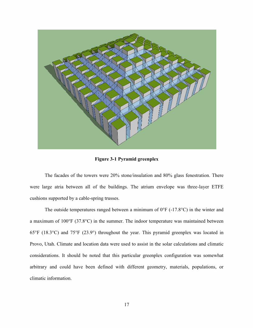
17

Figure 3-1 Pyramid greenplex

The facades of the towers were 20% stone/insulation and 80% glass fenestration. There

were large atria between all of the buildings. The atrium envelope was three-layer ETFE

cushions supported by a cable-spring trusses.

The outside temperatures ranged between a minimum of 0°F (-17.8°C) in the winter and

a maximum of 100°F (37.8°C) in the summer. The indoor temperature was maintained between

65°F (18.3°C) and 75°F (23.9°) throughout the year. This pyramid greenplex was located in

Provo, Utah. Climate and location data were used to assist in the solar calculations and climatic

considerations. It should be noted that this particular greenplex configuration was somewhat

arbitrary and could have been defined with different geometry, materials, populations, or

climatic information.

18

3.2 Spreadsheet Description

The spreadsheet program developed for this research computed the annual HVAC energy

demands for the greenplex with a conditioned atrium. The spreadsheet program consisted of 15

separate sheets. The first sheet was labeled the "Constants" sheet. The next 12 sheets were

monthly sheets, one for each month. The "Annual" sheet compiled the information from each of

the monthly sheets. The final sheet was the "Reference" sheet. Equations 3-1 to 3-12, Figure 3-3,

and the data included in Tables 3-4 to 3-9 are from ASHRAE's Fundamentals handbooks

(ASHRAE 2001; ASHRAE 2013). The rest of the equations listed in this chapter were developed

from specific applications of Fourier's Law (conduction), Newton's Law of Cooling (convection),

and specific heat mass flow rate equation (ventilation). Fourier's Law and Newton's Law of

Cooling were implemented as resistor models (Incropera et al. 2011).

3.2.1 Constants Sheet

The values entered on the "Constants" sheet corresponded to values that were constant for

the model. These values included building geometry, material thermal properties, and some

location information. For example, the following values were used for the pyramid greenplex:

lat = location latitude = 40.2 degrees north

L = tower length = 50m

W = tower width = 50m

Afloor = floor area = 9,450,000m2

Vtowers = total volume of all 100 towers = 3.78x107 m3

Vatrium = volume of the atrium = 3.34x107 m3

Rconv.i = R-value for convection inside the buildings = 0.2m2-K/W

Rconv.a = R-value for convection inside the atria = 0.75m2-K/W

19

Rconv.o = R-value for convection outside = 0.05m2-K/W

Rwall = R-value for conduction through wall = 2.5m2-K/W

Rroof = R-value for conduction through roof = 5.0m2-K/W

Rglass = R-value for conduction through glass = 0.366m2-K/W

RETFE = R-value for conduction through ETFE = 0.55m2-K/W

αwall = absorptivity of the wall = 0.7

τglass = transmissivity of glass = 0.93

τETFE = transmissivity of ETFE = 0.45

Δ = percentage of air volume changed each hour = 0.35ch/hr

ρair = density of air = 1.015kg/m3

cp = specific heat of air = 1.007kJ/kg-K

pglass = percentage of facade that is "glass" = 80%

pwall = percentage of facade that is "wall" = 20%

Awall.a.i = opaque wall area inside the atrium in section i = 168,000m2

Awin.a.i = window area inside the atrium in section i = 672,000m2

AETFE.t = total tilted ETFE area = 312,340m2

AETFE.v = total vertical ETFE area = 82,200m2

Awall.i = opaque wall area facing in direction i = 17,000m2

Awin.i = window area facing in direction i = 68,000m2

Aroof = total roof area = 250,000m2

ΣETFE.t = tilted ETFE tilt angle = 28.1°

ΣETFE.v = vertical ETFE tilt angle = 90°

Σroof = roof tilt angle = 0°

20

The latitude (lat) for Provo, Utah is 40.2 degrees north. This is entered as positive for

northern latitudes and negative for southern latitudes.

Several geometric properties were calculated from the dimensions given in Section 3.1

including the: length (L), width (W), total floor area (Afloor), tower volume (Vtowers), and atrium

volume (Vatrium). Additionally, wall, window, roof, and atrium envelope surface areas, facing

directions, and tilts were determined and listed in Tables 3-1, 3-2, and 3-3.

Table 3-1 Atrium Section Panel Geometric Information

Roof Wall North East South West North East South West

Tilt [°] 28.1 28.1 28.1 28.1 90 90 90 90 Direction [°] 0 90 180 270 0 90 180 270 Areas [m2] 78085 78085 78085 78085 20550 20550 20550 20550

Table 3-2 Tower Wall and Window Areas in Each Atrium Section

North East South West

Wall Area [m2] 168000 168000 168000 168000 Window Area [m2] 672000 672000 672000 672000

Table 3-3 Exposed Tower Geometric Information

Walls Roof

North East South West Tilt [°] 90 90 90 90 0

Direction [°] 0 90 180 270 180 Wall Areas [m2] 17000 17000 17000 17000 250000

Window Areas [m2] 68000 68000 68000 68000 -

The indoor convection resistance values (Rconv.i) were set based off information from a

paper by Awbi (1998). The outside convection resistance (Rconv.o ) was calibrated using a CFD

analysis with a wind speed of 2.0 m/s that will be discussed in Chapter 6. The CFD values for the

21

outside resistance coefficient was compared to several empirical convection results (see Figure

3-2) from several sources. (ASHRAE 2001; ASHRAE 2013; Incropera et al. 2011). The atrium

coefficients were assumed to be between inside and outside resistance values because the atrium

is shielded from the outside winds however its larger volume and ventilation rates allow for

larger convection currents than typically occur inside a normal space. (Gritch and Eason 2010)

Figure 3-2 Comparison of several different convection correlations.

The wall resistance value (Rwall) refers to the portions of the tower facade that are opaque

and they were assumed to have a layer of masonry (R = 0.15), an air gap (R = 0.18), a layer of

wood (R = 0.14), a layer of foam insulation (R = 1.95), and a layer of gypsum sheetrock (R =

0.08). Each layer can be added together to get a total conduction resistance value (Rwall =

2.50m2-K/W). The resistance value used to represent a 7/8 inch thick panel of insulated glass

0.01

0.1

1

10

0.01 0.1 1 10 100

Con

vect

ion

Res

ista

nce

Val

ues (

R )

[m2K

/W]

Wind Velocity [m/s]

Flat Plate Parallel Flow Laminar

Flat Plate Parallel Flow Turbulent Local Flat Plate Parallel Flow Heat Flux

Flat Plate Parallel Flow Turbulent Total 2013 Laminar Perpendicular Plate

Noncircular Cylinders

Circular Cylinders

Aligned Cylindar Bank

Staggered Cylinder Bank

Simplified Vertical Surface 2001

Rough Estimate

CFD Analysis

Power (CFD Analysis)

22

(Rglass) was 0.366m2-K/W. The roof resistance value (Rroof) was assumed to be a green roof and

consist of 12 inches of soil (R = 1.59), at least 4 inches of concrete (R = 0.15), an air space (R =

0.18), 6 inches of insulation (R = 3.00), and a layer of sheetrock (R = 0.08) with a total resistance

of 5.00m2-K/W. The resistance value for ETFE (RETFE) represents a three-layer ETFE cushion

from Vector Foiltec which equals 0.55m2-K/W (Winser 2004).

The radiative absorptivity of the opaque tower facade (αwall) was set at 0.70 to represent

the absorptivity of a light-gray masonry surface. The transmissivity of the glass windows (τglass)

were 0.93, which is standard for glass. The three-layer ETFE cushion used in the model had one

layer of white ETFE used to diffuse the light in the atrium. This white ETFE cushion had a

transmissivity (τETFE) of 0.45.

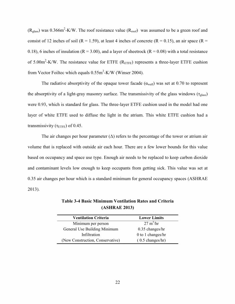
The air changes per hour parameter (Δ) refers to the percentage of the tower or atrium air

volume that is replaced with outside air each hour. There are a few lower bounds for this value

based on occupancy and space use type. Enough air needs to be replaced to keep carbon dioxide

and contaminant levels low enough to keep occupants from getting sick. This value was set at

0.35 air changes per hour which is a standard minimum for general occupancy spaces (ASHRAE

2013).

Table 3-4 Basic Minimum Ventilation Rates and Criteria (ASHRAE 2013)

Ventilation Criteria Lower Limits Minimum per person 27 m3/hr

General Use Building Minimum 0.35 changes/hr Infiltration

(New Construction, Conservative) 0 to 1 changes/hr ( 0.5 changes/hr)

23

3.2.2 Monthly Sheets

The monthly sheets required month-specific information and performed calculations for

one "design day" in each month. The design day was the 21st day of each month and it

conservatively approximated the two weeks before and the two weeks after the design day. All of

the thermal loads on the buildings were calculated at each hour of the design day for the different

control volumes. The monthly sheets ultimately calculated the greenplex HVAC energy demand

for the whole design day. Each month sheet was subdivided into an input block, an atria block, a

tower block, and a summary block.

The input block contained month-specific input information as well as some general

information transferred from the "Constants" sheet. As an example, the following values were

used in the "July" monthly sheet in addition to the values used in Section 3.2.1:

A = apparent solar irradiation = 1085W/m2

B = atmospheric extinction coefficient = 0.207

C = parameter depending on dust and moisture content of atmosphere = 0.136

ρg = ground reflectivity = 0.15

CN = clearness number = 1.0

δ = declination of the earth = 20.57deg

Tatrium = average temperature in the atrium = 23.89°C

Tin = average temperature inside the towers = 23.89°C

Thigh = daily outside high temperature = 37.78°C

Tlow = daily outside low temperature = 21.18°C

The first six values in this section (A, B, C, ρg, CN, δ) were used in the atria and tower

blocks to calculate the amount of solar radiation incident upon different surfaces in the model.

24

Table 3-5 includes the values for A, B, C, and δ for the 21st day of each month. These values

were used in conjunction with the temperature information above to solve for surface

temperatures, and to ultimately determine the heat transfer rates between the greenplex and the

surrounding environment.

Table 3-5 Solar Parameters for the 21st Day of Each Month (ASHRAE 2001)

Month Eo δ A B C

W/m2 deg W/m2 Jan 1416 -20.00 1230 0.142 0.058 Feb 1401 -10.80 1215 0.144 0.060 Mar 1381 0.00 1186 0.156 0.071 Apr 1356 11.60 1136 0.180 0.097 May 1336 20.00 1104 0.196 0.121 Jun 1336 23.45 1088 0.205 0.134 Jul 1336 20.60 1085 0.207 0.136 Aug 1338 12.30 1107 0.201 0.122 Sep 1359 0.00 1151 0.177 0.092 Oct 1380 -10.50 1192 0.160 0.073 Nov 1405 -19.80 1221 0.149 0.063 Dec 1417 -23.45 1233 0.142 0.057

The atria block balanced the heat transfer between the buildings and the outside

environments through the atrium for each hour of the design day. It specifically calculated the

surface temperatures of the tower walls inside the atrium, and determined how much solar heat

conducted into the towers and how much convected into the atrium. The outside temperature

(Tout) for each hour of the day is determined from Equation 3-1:

(3-1)

where Tlow is the low temperature for the design day, Thigh is the high temperature for the day,

and PDT is the percentage of the daily temperature range determined from Table 3-6 for each

hour of the day.

25

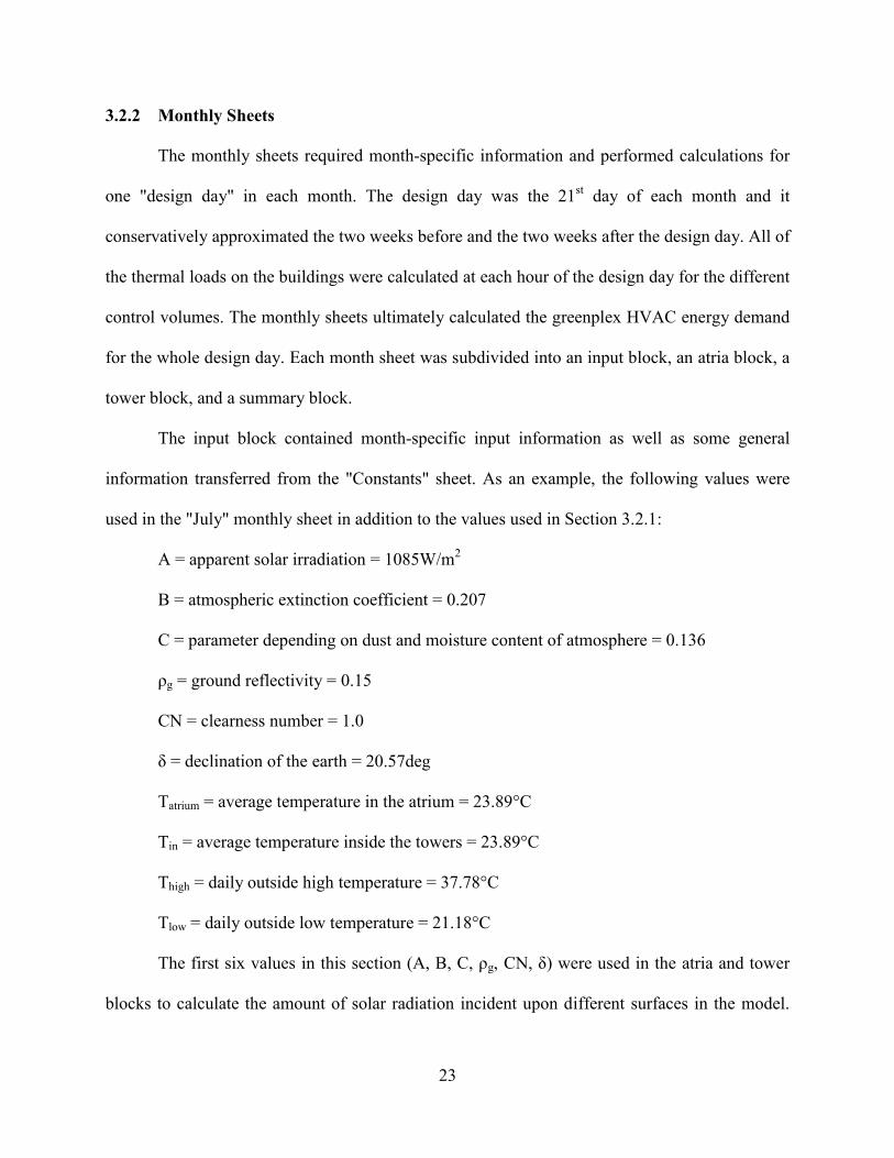
Table 3-6 Percentage of Daily Temperature Range (PDT) (ASHRAE 2013)

Time (h) % Time (h) % Time (h) % 1 13 9 29 17 90 2 8 10 44 18 79 3 4 11 61 19 66 4 1 12 77 20 53 5 0 13 89 21 42 6 2 14 97 22 32 7 7 15 100 23 24 8 16 16 97 24 18

The solar geometry angles shown in Figure 3-3 (ASHRAE 2013) must be determined.

The hour angle (H) in degrees is calculated with Equation (3-2:

(3-2)

where t is the time of day in hours. The height of the sun in the sky or solar altitude (β) is

calculated from Equation 3-3:

(3-3)

where lat is the site latitude and δ is the declination.

Figure 3-3 Solar geometry angles.

26

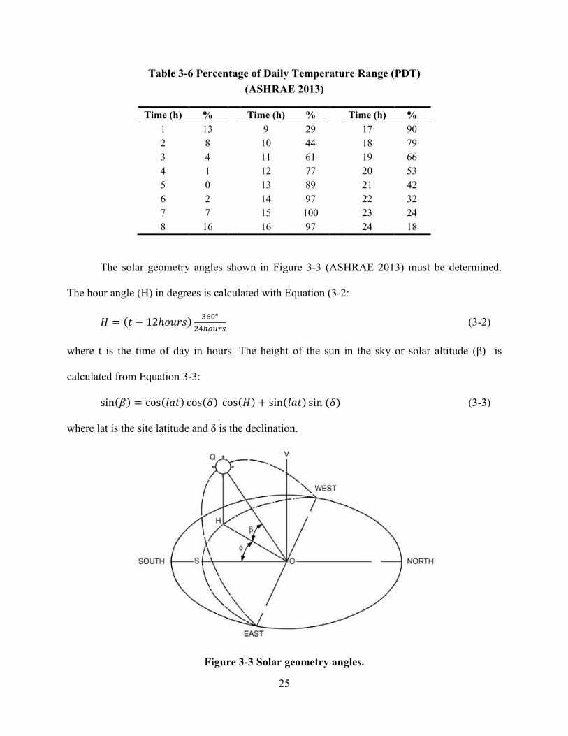
The solar azimuth (ϕ) can also be calculated from Equation 3-4:

(3-4)

where δ is the Earth's declination in degrees. The surface solar azimuth (γ) can be determined

from Equation 3-5:

(3-5)

where ψ is the surface facing azimuth in degrees (south is 0°, east is -90°, and west is 90°).

Finally, the surface-solar incident angle (θ) can be calculated from Equation 3-6:

(3-6)

where Σ is the surface's tilt from horizontal in degrees and β is calculated from Equation (3-3.

After the solar geometry angles have been determined, they are used to determine the

amount of solar radiation that makes it through the atmosphere to the surface of the earth. The

direct normal irradiance is calculated from Equation 3-7:

(3-7)

where CN is the clearness number, A is the apparent solar radiation, B is the atmospheric

extinction coefficient, and β is the solar altitude. The sun is only shining if it is above the horizon

(β > 0). The clearness number (CN) represents how clear the sky is. For a perfectly clear day CN

would be equal to one, and for a cloudy day CN would be about 0.5. Surface direct irradiance

(ED) is the amount of direct beam solar radiation incident upon a surface at a given time and

location. It is calculated from Equation 3-8:

(3-8)

27

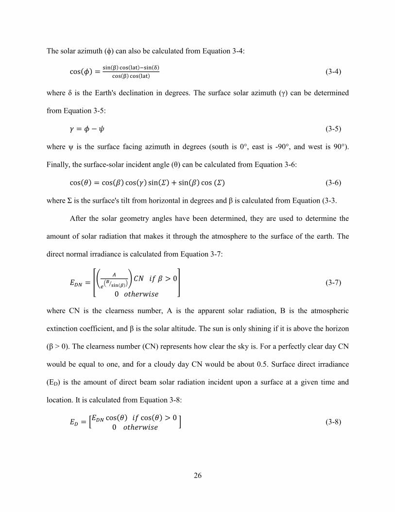
which is only valid if the sun is in front of a surface (i.e. cos(θ) > 0). Y is the ratio of sky diffuse

on vertical surface to sky diffuse on horizontal surface. Y is calculated from Equation 3-9:

(3-9)

where θ is the surface-solar incident angle. The diffuse solar irradiation (Ed) refers the sunlight

that is scattered as it enters the atmosphere and lights up the sky. The sky shines in all directions

and is the major source of radiation gain on shaded surfaces. It is defined by Equation 3-10:

(3-10)

where C is the atmospheric parameter and Σ is the surface tilt. Sometimes a significant amount of

radiation is reflected from the ground onto a surface. This ground-reflected solar radiation is

determined from Equation 3-11:

(3-11)

where ρg is the ground surface reflectivity (typically 0.2 for a standard mixture of ground

surfaces). Finally, the total surface irradiance can be determined by summing the contributions

from direct beam solar, diffuse solar, and ground reflected solar radiation in Equation 3-12:

(3-12)

This total incident solar heat rate Et needs to be determined for each surface in the model (walls,

windows, roofs, ETFE, etc.) for each hour of the design day.

Once the incident solar heat rate was calculated, the amount of radiation transmitted

through the ETFE envelope was determined from Equation 3-13:

(3-13)

where EETFE is Et for an ETFE envelope surface, and τETFE is the transmissivity (or transparency)

of the ETFE. Then the solar energy transmitted into the atrium needed to be divided between the

28

tower walls inside the atrium. This was done by multiplying the energy into each atrium section

by an ETFE envelope to interior wall area ratio in Equation3-14:

(3-14)

The value of Ewall represents the average amount of energy from the sun that makes it into the

atrium and is absorbed into or transmitted through a unit area of wall or window material.

The next section of the atrium block calculated the thermal forces including incident solar

radiation and ventilation from Equations 3-15 to 3-17:

(3-15)

(3-16)

(3-17)

These values were used in Equations 3-18 and 3-19 to determine the surface temperatures

of the tower walls and windows inside the atrium:

(3-18)

(3-19)

Finally, the wall and window surface temperatures were used to determine the amount of

heat transferring through the components of the greenplex. The heat conducting into the towers

is calculated from Equations 3-20 and 3-21:

(3-20)

(3-21)

29

The heat convecting into the atrium is calculate from Equation 3-22:

(3-22)

where n is number of surfaces (windows and walls) inside the atrium.

The tower block balances the heat transfer between the towers and the outside

environment through the exterior tower walls and windows. Equations 3-2 through 3-12 were

used to determine the solar radiation incident on each of the exterior walls. The heat flux of

incident solar radiation absorbed was calculated from Equation 3-23:

(3-23)

where Et is the incident solar heat rate on the exterior wall surfaces of the towers. Then the

outside wall surface temperature was calculated from Equation3-24, and the outside window

surface temperature was calculated from Equation 3-25:

(3-24)

(3-25)

With the outside surface temperatures, the heat rate into the towers through the exterior walls

was calculated from Equations 3-26 and 3-27:

(3-26)

(3-27)

Note that heat fluxes could be computed by first leaving the areas out of Equations 3-26

and 3-27, and then the total heat rate could be determined by multiplying the heat flux by the

30

total wall or window area according to Equation 3-28:

(3-28)

The summary block compiled the information generated from the atria and tower blocks,

and accounted for internal heat gains from people, lights, and equipment. It added all of the

hourly information from each of the other blocks into a final daily heating and air-conditioning

energy demand. The average metabolic heat rates for a person present in the building for each

hour were entered into one column. Then equipment and light heat rates per floor area were

entered into the next two columns for each hour of the day. The total heat generated inside the

towers by the people can be determined from Equation 3-29:

(3-29)

where npeople is the number of people inside the pyramid greenplex and qmet is the average

metabolic heat rate per person in a given hour. The total heat generated by the equipment and

lights can be determined from Equations 3-30 and 3-31:

(3-30)

(3-31)

where q''eq is the average heat rate for the equipment in the building per floor area and q''lights is

the average lighting heat rate per floor area for the whole building (see Table 3-7). These values

could be determined alternatively by assigning space uses throughout the building and then

choosing appropriate equipment and lighting heat rates for each space use. The total heat rate due

to equipment and/or lights could be calculated for each space usage type from Equations 3-30

and 3-31. The total heat rate for lights and equipment in the whole pyramid greenplex could be

determined by summing up all of the heat rates for all of the individual spaces.

31

The conduction heat rates into the towers were computed by summing the heat rates from

each of the exterior walls and windows. The conduction rates through the windows and walls

into the towers from the atrium (see Equations 3-20 and 3-21 from the atrium block) were also

combined. The solar radiation heat rates into the towers were computed for the sunlight that was

transmitted through the atrium and interior windows and exterior windows. Finally, the tower

ventilation heat rates from adjusting the temperature of air from outside to match the tower air

temperature were computed using equation 3-32:

(3-32)

where Vt is the volume of the towers, Δt is the percentage of the tower air volume that it

exchanged every hour, ρair is the density of air, and cp is the specific heat of air.

Each of these hourly totals can be summed up for a total heating energy demand for the

hour. Positive values indicate the amount of thermal energy the air-conditioner needs to remove

from the system and negative values indicate the amount of energy the heater must supply to the

system to maintain the temperatures in the towers and atria. The total daily energy demand is the

sum of the absolute value of the hourly total heat rates for the towers and the atrium.

3.2.3 Annual Sheet

The last calculation sheet was the annual sheet. It took the total daily energy demand

heating and air-conditioning values from each of the month sheets and calculated a total annual

heating/air-conditioning energy demand. This was done by integrating a linear interpolation

between each of the design days for the whole year from Equation 3-33:

(3-33)

32

where Ei is the total energy demand for design day i, Ei+1 is the total energy demand for design

day i+1, and nDi is the number of days in month i. The annual HVAC energy demand was also

divided by the total floor area. This energy per floor area parameter can be used to compare the

energy performances of buildings of different sizes.

3.2.4 Reference Sheet

The reference sheet had several tables of condensed data from the ASHRAE manuals and

material specification sheets (ASHRAE 2013; Vector Foiltec 2012; Winser 2004). These were to

help a designer determine some basic input information. Examples of how to calculate

conduction resistance values for layered walls similar to the calculation of Rwall and Rroof in

Section 3.2.1 were also included. Table 3-4 is included on the references sheet as well as the

tables included below. The majority of the information included in Tables 3-7 through 3-9 came

from the ASHRAE manual Fundamentals 2013. Some more specific information, or at least

information about more unique materials, was compiled from several online resources and

technical papers. (ASHRAE 2013; Awbi 1998; Winser 2004)

Table 3-7 Heat Sources Based on Space Use

Space Use Type Area per

Person [m2] Light per area

[W/m2] Appliances per Area [W/m2]

Office 18 18 5 to 22 Residential [High] 28 21 5 Residential [Mid] 45 18 5 Residential [Low] 75 15 5

Hotel 5 10 5 Hospital [max] 15 16 5 to 140

Restaurant 2 10 to 20 5 to 15 Retail 2 10 to 20 5 School 2 15 to 25 5

33

Table 3-8 Human Metabolic Heat Generation Rates

Activity Level Metabolic Heat

[W/person] Sleeping 40 Standing 70 Walking 115 Cleaning 115 to 200

Hard Work 120 to 280 Basketball 290 to 440

Table 3-9 Material Thermal Properties

Materials R-Values [m2K/W]

Absorption (α)

Transmission (τ)

Glass Single Pane 0.150 - 0.90

Insulated Glass 7/8 inch 0.366 - 0.90 Low-E Glass 0.431 - 0.90 Low-E with Argon 0.766 - 0.90 ETFE

-

Single Layer 0.200 - 0.92 Three Layer Cushion 0.550 - 0.85 Three Layer White 0.550 - 0.45 Walls

Brick (4inch) 0.145 0.60 - Concrete Block (8 inch) 0.193 0.60 - Wood 0.135 0.4 to 0.7 - Insulation 3inch 1.930 - - Insulation 6inch 3.340 - - Sheet rock 0.080 - - Steel/Aluminum Siding 0.100 0.2 to 0.80 - Air 0.176 - 1.00 Roofing

Asphalt (shingles) 0.100 0.85 - Soil (per inch) 0.140

-

Grass 0.50 -

34

3.3 Chapter Summary

A spreadsheet model was developed specifically to determine the annual HVAC energy

demands of a 100-building greenplex with an atrium conditioned to the same temperature as the

towers. The conditioned atrium spreadsheet model consisted of 15 sheets: a "Constants" sheet,

12 month sheets, an "Annual" sheet, and a "Reference" sheet. The "Constants" sheet contained

all of the information in the model that was constant throughout the year including: geometric,

location, and material data. Each month sheet determined the HVAC energy demands for the 21st

day of that month. The "Annual" sheet used the daily HVAC energy demands from each of the

month sheets to determine a total annual HVAC energy demand.

35

4 NO-ATRIUM SPREADSHEET MODEL

The no-atrium spreadsheet model is more simple application of ASHRAE's RTS method

without the time series information included (ASHRAE 2013). This chapter presents the

information used to develop the no-atrium spreadsheet model. The key feature of this model is

that there is no atrium between the buildings. This chapter describes how the no-atrium

spreadsheet model was setup differently from the conditioned atrium spreadsheet model.


Many aspects of the no-atrium spreadsheet were similar to the Conditioned Atria

Spreadsheet Model in Chapter 3. This model consisted of 15 sheets, which included the

"Constants" sheet, the 12 month sheets, the "Annual" sheet, and the "Reference" sheet. Since so

much of the separate models were similar to each other, only differences will be discussed.

The "Constants" sheet had all of the same values as the conditioned atrium spreadsheet

model except for the atrium parameters. The monthly sheets had the most significant differences.

These sheets were set up with only two blocks: an input block and a tower block. The input

block consisted of several values from "Constants" sheet and a few month-specific values. The

tower block was where all of the calculations for each design day took place. The tower block

was set up to represent several towers at once, but if the towers were significantly different it

would be more advantageous to copy the tower block from the first tower and adjust it for

36

successive towers. The tower block was divided into several sections with one section per

surface (wall or roof). This allowed additional walls or roof sections to be inserted easily, as

needed. In each section the incident solar radiation was calculated using Equations 3-2 through

3-12 in Chapter 3. The incident solar radiation was used with Equations 3-24 and 3-25 to

determine the wall and window surface temperatures. A shadow parameter was introduced where

the percentage of a wall that was in the shade was specified. Determining actual shading can be a

very complicated process depending on diffuse solar radiation and surface reflectivity. These

shading values were estimated by drawing the model in Google Sketchup (Trimble et al. 2013)

and using the built-in shading rendering capability to visually estimate the percentage of each

wall that was shaded. This was done for each hour of the twelve design days. Equations 3-26 and

3-27 were used to determine the conduction rates through the walls and windows. The solar

radiation incident on the windows was used to determine the radiation transmitted through the

windows. The window-transmitted solar was assumed to get absorbed within the buildings.

The last section of the tower block finished off the design day calculations. It included

the calculations for the internal gains from people, lights, and equipment. It also accounted for

the ventilation energy demand using Equation 3-32. Finally, it summed all of the heat rates from

each of the sections to determine an hourly total heat rate. The absolute value of the total hourly

heat rates were summed for the whole day to determine the total design day HVAC energy

demand.

4.2 Chapter Summary

The no-atrium spreadsheet model was much simpler than the atrium models because no

atrium calculations needed to be performed and the wall and window surface temperatures could

be easily determined from Equations 3-24 and 3-25. The no-atrium spreadsheet model was also

37

designed to handle very different building designs and configurations because the wall sections

and the tower blocks were more modular. Additional walls, roofs, or window surfaces could be

added to the model by copying more wall sections into the tower block and adjusting some of the

formulas to include them. Several different towers could be analyzed at once be copying the

tower block and adjusting parameters in the copied blocks to represent the other additional

towers.

38

5 UNCONDITIONED ATRIUM SPREADSHEET MODEL

Determining annual HVAC energy demands on a typical building is usually

straightforward (see Chapter 4). Including an atrium in the analysis increases the complexity of

the analysis because of the possibility of thermal coupling between the atrium, inside, and

outside environments. This chapter presents the equations and information used to develop the

unconditioned atrium spreadsheet model. The key feature of this model is that the average atrium

temperature is unknown and coupled with the atrium solar gains, conduction rates, and

ventilation rates. This chapter describes the unique aspects of the unconditioned atrium

spreadsheet setup.


Many aspects of the unconditioned atrium spreadsheet were similar to the conditioned

atrium spreadsheet in Chapter 3. The unconditioned atrium spreadsheet model consisted of 15

sheets, which included the "Constants" sheet, the 12 month sheets, the "Annual" sheet, and the

"Reference" sheet. The "Constants," "Annual," and "Reference" sheets were identical to the

conditioned atrium model. Only the differences in the 12 month sheets will be discussed.

The month sheets were set up in a series of five blocks similar to the Conditioned Atrium

Model. There was an input, atrium, tower, and summary block with an added resistance matrix

block for the greenplex. The input block did not have a value for the atrium temperature. The

39

tower block was identical between the unconditioned and conditioned atrium models. The only

difference in the summary block was there was no atrium energy demand column because the

atrium energy demand was zero.

This case maintained the tower temperature at a comfortable range throughout the year,

but the atrium not directly conditioned and the atrium temperature could change throughout the

design day. On the month sheets, the average atrium temperature and the tower wall and window

surface temperatures had to be determined. To complicate things, these temperatures were

coupled with conduction rates through walls, windows, and ETFE, the solar loads, and

ventilation rates in the atrium. A system of linear equations (see Equation 5-1) was developed to

solve for atrium wall and window surface temperatures as well as the average atrium air

temperature.

(5-1)

The resistance matrix block was composed of resistances for the nine different

temperature degrees of freedom (DOF) (four atrium-section wall surface temperatures, four

atrium-section window surface temperatures, and an average atrium air temperature). The

surfaces were assumed to be uncoupled from each other but coupled with the average atrium

temperature. The formulas for each surface DOF are given by Equations 5-2 and 5-3:

(5-2)

(5-3)

where Rii is the matrix resistance value for surface i, Ai is the area of surface i, and Ri is the

resistance value for surface i. The ventilation DOF is defined by Equation 5-4:

(5-4)

40

where the Vat is the volume of the atrium, Δat is the percent of the atrium volume that is replaced

every hour, ρair is density of air, and cp is the specific heat of the air. These values (Rii, Ri,at and

Rat,at) were put into the resistance matrix R given by Equation 5-5:

(5-5)

The load vector (F) was generated for each hour of the day. The thermal load on the wall

surfaces inside the atrium depends on the radiative thermal load from the sun and the conductive

thermal load from the inside of the tower. The load vector values for the wall surfaces inside the

atrium is given by Equation 5-6:

(5-6)

where α is the absorptivity of the wall surface i, Ei is the incident solar on wall i (see Equation 3-

14), and Ri is the conductivity of the wall surface i. The load vector values for the window

surfaces inside the atrium is given by Equation 5-7:

(5-7)

where Ri is the conductivity of window i. Note that there is no solar load on the surface of the

window only conductive loading from inside the towers. This is because any radiation loads get

transferred through the window and very little energy is absorbed by the window. Finally, the

load vector value for the atrium ventilation DOF is given by Equation 5-8:

(5-8)

41

The resistance matrix was inverted and multiplied by the load vector to get the average

surface temperatures of each of the walls and windows as well as the average air temperature in

the atrium (see second part of Equation 5-1). These surface temperatures could then be used to

determine the heat rates into the towers from Equations 3-26 and 3-27.

5.2 Development

The series of linear equations for the unconditioned atrium spreadsheet model that

balanced the heat transfer rates through the atrium were developed using a resistor model. The

resistor model specifically accounted for conduction, convection, radiation, and ventilation using

Fourier's Law, Newton's Law of Cooling, ASHRAE's solar formulas, and the specific heat

equation (ASHRAE 2013; Incropera et al. 2011). The resistor model consisted of several

temperature nodes connected to each other by thermal resistors (see Figure 5-1). The heat rates at

each node must balance. There were four main node types: indoor air temperature, wall or

window surface temperature on the atrium side, average atrium air temperature, and outside air

temperature. There are also six thermal resistor types: wall, window, ETFE, indoor convection,

atrium convection, and outside convection. In addition, thermal forces were applied through

solar radiation incident upon the atrium walls and ventilation into the atrium air.

Figure 5-1 Basic resistor model

A linear equation was developed from each unknown node (see Equation 5-9 for node

Ts,i). These equations were then rearranged in terms known and unknown nodal information (see

42

Equation 5-10). The coefficients of the unknown temperature nodes became the resistance values

in the resistance matrix block (see Equations 5-2 to 5-5). All known information was put into the

load vector (F) (see Equations 5-6 through 5-8). And the unknown atrium and surface

temperatures could be determined with Equation 5-1.

(5-9)

(5-10)

5.3 Chapter Summary

The unconditioned atrium spreadsheet model was nearly identical to the unconditioned

atrium spreadsheet model presented in Chapter 3. The sheets were identical except for the 12

month sheets. The main differences on the monthly sheets were the addition of the resistance

matrix block and the formulas used in the atrium block. It required the development of a series of

linear equations based on Fourier's Law (conduction), Newton's Law of Cooling (convection),

and the mass flow rate specific heat equation. These linear equations with the solar calculations

from ASHRAE allowed the average atrium air temperature and the wall and window surface

temperatures to be determined. The wall, window, and atrium temperatures were used to

determine the heat transfer rates into the towers.

43

6 CALIBRATION OF SPREADSHEET MODELS WITH CFD

Computational fluid dynamics (CFD) models have the capability of evaluating how

different fluid currents are caused by obstructions and how those currents affect the heat transfer

or forces on the obstructions. This chapter focuses on the CFD modeling of the no-atrium case.

The CFD model and assumptions are explored followed by the results and limitation of the CFD

analysis. The CFD results are compared to the spreadsheet and hand calculated results.

6.1 CFD Model Definition and Assumptions

A more detailed CFD model was developed to help calibrate the exterior convection rates

in the spreadsheet model. The greenplex without atria was modeled in a simulated wind tunnel

scenario to determine what heat rates would result from different wind velocities and

temperature differences between inside and outside. The CFD model consisted of 100 square

prismatic boxes representing the towers inside a large wind tunnel box.

The model was created, meshed, and analyzed with the Star-CCM+ software

(MacDonald 2014). Star-CCM+ includes a built-in CAD module that can be used to generate the

geometric information for the model. Star-CCM+ uses three datasets to define and analyze a

model (continua, regions, and interfaces). The continua dataset includes the meshing and physics

subsets that define how the model is discretized and what physical/mathematical models should

be used to develop a solution. The physics continua subset also includes information on the

44

initial conditions for the solution. The regions dataset includes the geometry, mesh parameters,

physics parameters, and some boundary condition values for each of the control volumes in the

model. The interfaces dataset includes meshing and physics information about the boundaries

between the wind tunnel and tower control volumes (the tower walls).

Post-processing was done using the reports, monitors, plots, and scenes datasets. The

reports datasets calculated overall information, like total greenplex heat transfer, using the

individual element values. The monitors datasets were set up to keep track of the report

information at each iteration, and the plots datasets were generated from the monitored

information. The scenes dataset presents visual representations of the data.

6.2 Procedure

The model geometry was created with the built-in CAD module and geometric boolean

operations. This had to be done carefully to ensure that the resulting volumes were feasible and

didn't have any orphaned surfaces or edges. The geometry was transferred to the regions dataset

where the boundaries between the towers and wind tunnel were defined along with the mesh and

physics continua subsets.

The meshing algorithms used to discretize the model were: the surface remesher, the

polyhedral mesher, and the prism layer mesher. The surface remesher discretized all of the

surfaces of the model into sets of nearly equilateral triangles. It then conducted several

refinements and optimizations to make the triangular surface mesh as uniform as possible. The

polyhedral mesher divided the volumes into multi-sided, nearly spherical, polyhedra with

diameters as close to the base size as possible. The prism layer mesher created prismatic

polyhedral elements starting from each of the wall and roof interfaces in the model. This prism

layer was sized to accurately capture the boundary layer development along the walls of the

45

model. The prism layer mesher and the polyhedral mesher were optimized together to adequately

transition from a primarily two-dimensional flow regime next to a wall to a three-dimensional

turbulent flow away from the boundaries (see Figure 6-1). A volumetric control was specified

that refined the volume mesh in the area right around the towers. More specific meshing

information was defined under the regions and interfaces properties.

Figure 6-1 Volume mesh on a horizontal cross section through the city.

There were two separate physics continuum subsets created to be used for tower and

wind tunnel control volumes, respectively. They differed only in the initial conditions. The

physics continuum subset algorithms selected were: Three Dimensional, Gradients, Steady, Ideal

Gas, Segregated Flow, Segregated Fluid Temperature, Turbulent, Reynolds-Averaged Navier-

Stokes, K-Omega Turbulence, and SST K-Omega. The default values were used for the

reference values and initial conditions with the exception of the temperature and velocity initial

conditions in the wind tunnel. The velocity was set to a specified magnitude (initially 2.0m/s but

later adjusted as shown in Table 6-1) and the wind tunnel temperature was set to 255.4K (0.0°F).

46

The physics properties were further defined for each of the regions and the interfaces between

the regions. The tower/wind tunnel interface boundary conditions were specified as a baffle

interface. The baffle interface was further modified to be a conductive interface with a

conduction resistance of 0.471m2K/W. This value was determined using parallel resistance given

by Equation 6-1:

(6-1)

where Awall is the total surface area of all of the wall in the city, Awindow is the total surface area

of all of the glass, and Aroof is the area of all of the roof, and Rwindow is equal to Rglass.

The model was meshed at this point. The surface meshing routine was executed and the

model was checked for errors. Then the volume meshing routine was executed. Next, the wind

tunnel surfaces were separated, renamed, and assigned boundary conditions. The boundary

conditions included: velocity inlet, pressure outlet, slip wall for the top, symmetry plane for the

side surfaces, and no-slip wall for the ground surface. The physics boundary conditions for each

of these wind tunnel surfaces were further defined. An air velocity and temperature that matched

the wind tunnel velocity and temperature initial condition was specified for the velocity inlet.

The surface temperatures of the other wind tunnel boundary surfaces were specified to match the

wind tunnel initial air temperature.

Some user defined field functions were used in conjunction with the K-Omega

Turbulence algorithm to set and hold the temperature inside the towers. The field functions were

defined by Equations 6-2 and 6-3:

(6-2)

(6-3)

47

where Tcell is the cell, or element, temperature, Tset is the indoor temperature setting, C is a large

constant chosen to get the temperatures set quickly, Q is the volumetric heat rate, and dQ/dT is

the volumetric heat rate temperature derivative. The volumetric heat source option was selected

in the towers' physics conditions energy source options. The towers' volumetric heat source,

under their physics conditions category, was defined as the field function Q and the towers'

energy source temperature derivative was set as the field function dQ/dT. This method for

maintaining an air temperature was given in the user's manual for Star-CCM+ (CD-Adapco

2014).

Finally, some post processing information was defined before running the analysis. These

included scenes and reports datasets. Several scenes datasets were defined to view the geometry,

surface and volume meshes, and different solution results (air velocity vectors, air temperatures,

and surface pressures). The air temperature and air velocity scenes were set up with information

shown on a cut plane through the model (see Figures 6-1 and 6-5). The pressure information was

selected for the exterior surfaces of the towers. Heat transfer report datasets were created and

defined to determine the heat transfer rate through the walls of the towers from the point of view

of the towers and the point of view of the wind tunnel. This was done to ensure that the heat

transfer balanced on both sides of the wall. Then monitors and plots were created to record and

plot the heat transfer rates at each iteration.

6.3 CFD Model Results

Three different element base sizes were analyzed. The element base size in the wind

tunnel away from the greenplex was maintained at 20 meters. The element base size in the

greenplex and out to at least 100 meters surrounding the greenplex was set to 20, 10, and 5

48

meters for the 2.0 m/s velocity models as shown in Figure 6-2. Several velocities were analyzed

with the 5 meter base size mesh.

Figure 6-2 Plots of heat transfer rate for the city for different base size values.

Figure 6-3 Heat transfer rates for the greenplex vs. wind speed at 5 meter base size.

The data for the positive heat transfer dataset was exported and plotted as shown in

Figure 6-3. The flat sections of these plots were assumed to be converged, and the average

1

10

100

1000

0 100 200 300 400 500

Hea

t Tra

nsfe

r R

ate

[MW

]

Iteration

Base Size = 5m

Base Size = 10m

Base Size = 20m

10

30

50

70

90

110

130

150

0 200 400 600 800 1000

Hea

t Tra

nsfe

r R

ate

[MW

]

Iteration

V = 20m/s

V = 10m/s

V = 5.0m/s

V = 2.0m/s

V = 1.0m/s

V = 0.5m/s

V = 0.1m/s

49

conduction rates after convergence for the different air velocities are included in Table 6-1.

These values were used to calculate effective external convection coefficients for the greenplex.

Table 6-1 Greenplex Heat Transfer Rates for Different Wind Speeds.

Velocity [m/s]

Conduction Rate [MW]

0.1 22.81 0.2 34.39 0.5 55.90 1 78.23 2 89.70 5 106.91

10 117.49 20 124.86

Additionally, heat transfer scalar scenes and flow vector scenes were produced. (see

Figures 6-4 and 6-5). These were used to verify that the solution was reasonable. They were also

used in early models to find errors in the input parameters and analysis results.

Figure 6-4 Heat transfer rates through the walls from a 2.0m/s wind.

50

Figure 6-5 Horizontal flow vector plane showing flow around buildings. (wind direction is from bottom to top)

6.4 Limitations

There was one main limitation to the CFD analysis (computer memory) which caused

two major limitations to the model (element size and scope). The models were created, meshed,

and modified on a computer with a maximum of eight gigabytes (8GB) of memory. This

memory limit placed constraints on the element size and the model scope. The model file size

could only be 5.5GB before file modification became an issue. As a result, the maximum number

of elements was 13 million with 70 million faces. It should be noted that files this large required

more than 20GB of computer memory and up to 52 hours to complete each simulation. These

files had to be transferred to a supercomputer to run the simulation.

The model was very large (2000m wide by 4000m long by 800m high). The greenplex

was 725 meters wide and 280 meters tall. Typically, it is recommended that the wind tunnel is at

least six times as wide as the object, at least six times as long as the object, and at least five times

as tall as the object so that the wind tunnel walls do not interfere with the flow around the

51

greenplex (CD-Adapco 2014). These recommended values resulted in such a large model that it

was necessary to reduce the wind tunnel size to only 2.75 times the greenplex width, 5.5 times

the greenplex length, and 2.85 times the greenplex height. These reductions reduced the model

volume by 75%.

Initially, a maximum element size was set to twenty meters. This resulted in a small file

that could be run quickly but had major errors in the heat transfer values. Then a mesh

volumetric control was implemented that refined the mesh within 100 meters of the greenplex

(300 meters downwind). The elements within this volumetric control could have minimum base

size of five meters before file size constraints were reached.

Due to the element size limitations, the detail and complexity of the model was also

limited. For example, elements could not be sized small enough to capture data between floors or

solid wall and window facade differences. So tower floors were not modeled and window and

wall sections were modeled with effective values. (see Figure 6-1). The CFD analyses do not

include radiation models or analyses. This is mainly because the solar models require opaque

surfaces to absorb solar radiation and the mesh size did not permit useful or accurate modeling of

the different transparent and opaque surfaces in the model.

The atrium models were attempted in Star-CCM+ however, a large component of the heat

transfer was ventilation, especially in the unconditioned atrium. The mesh was not fine enough to

model intake and exhaust vents in the atrium. Ventilation (natural or forced) was not included in

the CFD analysis because it was very difficult to define correctly and more difficult to get the

solution to converge. Additionally, vent locations, sizes, velocities, pressures, etc. were not

known or defined.

52

6.5 Comparison with Spreadsheet and Hand Calculated Results

The CFD tower model was compared with a very basic hand calculated model and a non-

solar spreadsheet model. The hand calculated model used several different convection coefficient

correlations to determine a reasonable range of heat transfer rates for the CFD model and to help

with troubleshooting. The total greenplex heat transfer rate was computed from Equation 6-4:

(6-4)

where Qtotal is the total heat transfer rate for the whole greenplex, Rconv.o is a convection

correlation that is a function of wind velocity, and Reff is the value from Equation 6-1. Plots of

the greenplex heat rate using different convection correlations have been included in Figure 6-6.

The different convection correlations apply to very specific flow geometries and Reynolds

number ranges. For many of these empirical correlations, the greenplex's (or even a tower's)

Reynolds number was well above the valid Reynolds number range. The simplified vertical

surface convection correlation is from ASHRAE and is designed to conservatively approximate

the exterior convection due to both wind and buoyancy. It should also be noted that the

maximum value (2.767x108W) for the vertical axis of Figure 6-6 was the greenplex's heat

transfer rate if the inside and outside convection resistance values (Rconv.i and Rconv.o) were both

equal to zero.

Equation 6-4 can be rearranged to solve for Rconv.o as shown in Equation 6-5. The average

greenplex outside convection resistance values can be directly compared to the empirical

convection correlations as shown in Figure 6-7.

(6-5)

53

The non-solar spreadsheet was created from a no-atrium spreadsheet model. For this

model the solar gains and internal gains were set to zero. Furthermore, the outside and inside

temperatures were set at the same values that were used for the CFD and hand calculated models.

It was determined that the CFD model follows the trends of the different correlations but

is probably unconservative. Refining the mesh pushed the CFD solutions closer to the hand

calculations. It could converge towards a solution for the system if the mesh could be refined

more. Unfortunately, there was not enough computer memory on the systems used to create and

save the file to refine the mesh further.

Figure 6-6 Total greenplex heat transfer rate for a temperature difference of 65°F and several outside convection correlations.

10

100

0.01 0.1 1 10 100

Hea

t Tra

nsfe

r R

ate

[MW

]

Wind Velocity [m/s]

Flat Plate Parallel Flow Laminar Flat Plate Parallel Flow Turbulent Local Flat Plate Parallel Flow Heat Flux Flat Plate Parallel Flow Turbulent Total 2013 Laminar Perpendicular Plate


Circular Cylinders



Simplified Vertical Surface 2001 Rough Estimate

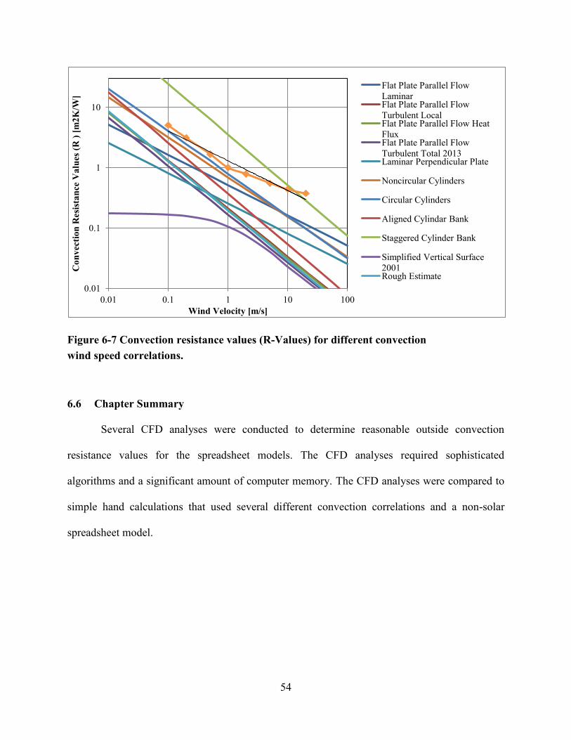
54

Figure 6-7 Convection resistance values (R-Values) for different convection wind speed correlations.

6.6 Chapter Summary

Several CFD analyses were conducted to determine reasonable outside convection

resistance values for the spreadsheet models. The CFD analyses required sophisticated

algorithms and a significant amount of computer memory. The CFD analyses were compared to

simple hand calculations that used several different convection correlations and a non-solar

spreadsheet model.

0.01

0.1

1

10

0.01 0.1 1 10 100

Con

vect

ion

Res

istan

ce V

alue

s (R

) [m

2K/W

]

Wind Velocity [m/s]

Flat Plate Parallel Flow Laminar Flat Plate Parallel Flow Turbulent Local Flat Plate Parallel Flow Heat Flux Flat Plate Parallel Flow Turbulent Total 2013 Laminar Perpendicular Plate


Circular Cylinders



Simplified Vertical Surface 2001 Rough Estimate

55

7 RESULTS AND DISCUSSION

The spreadsheet models presented in Chapters 3, 4, and 5 progressed through several

stages of calculations to determine total annual heating and cooling energy demands for their

specific atrium configurations. This chapter will present the energy demand and temperatures

from the three spreadsheet models. The major factors that contributed most significantly to the

energy demand and temperatures will be discussed further along with the limitations of these

models and areas of future research.

7.1 Energy Demand

Three greenplex configuration cases were examined with the spreadsheet analysis

programs. The design day results for the 12 design days for each of the three cases are presented

in Table 7-1 and Figure 7-1. The annual energy demand for the no-atrium case was 2093 GW-

hr/yr and the annual energy demand per floor area was 221.5 kW-hr/m2. In the conditioned

atrium analysis the annual energy demand was 1759 GW-hr/yr and the annual energy demand

per floor area was 186.1 kW-hr/m2. In the unconditioned atrium analysis the atrium temperatures

were not actively controlled or known. The atrium behaved mainly as an extra layer of insulation

from the towers and the annual energy demand was 1055 GW-hr/yr and the annual energy

demand per floor area was 111.5 kW-hr/m2. All of these values are within the range of energy

consumption values compiled by Wood and Salib (2012).

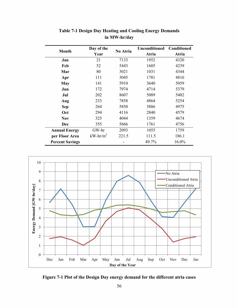
56

Table 7-1 Design Day Heating and Cooling Energy Demands in MW-hr/day

Month Day of the

Year No Atria

Unconditioned Atria

Conditioned Atria

Jan 21 7133 1952 4320 Feb 52 5443 1605 4239 Mar 80 3021 1031 4344 Apr 111 3045 1781 4816 May 141 5910 3640 5059 Jun 172 7974 4714 5379 Jul 202 8607 5089 5402 Aug 233 7858 4864 5254 Sep 264 5850 3886 4975 Oct 294 4116 2840 4579 Nov 325 4044 1359 4674 Dec 355 5666 1761 4756

Annual Energy GW-hr 2093 1055 1759 per Floor Area kW-hr/m2 221.5 111.5 186.1 Percent Savings - 49.7% 16.0%

Figure 7-1 Plot of the Design Day energy demand for the different atria cases

0

1

2

3

4

5

6

7

8

9

10

Dec Jan Feb Mar Apr May Jun Jul Aug Sep Oct Nov Dec Jan

Ene

rgy

Dem

and

[GW

-hr/

day]

Day of the Year

No Atria Unconditioned Atria Conditioned Atria

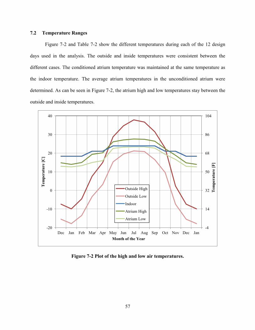
57

7.2 Temperature Ranges

Figure 7-2 and Table 7-2 show the different temperatures during each of the 12 design

days used in the analysis. The outside and inside temperatures were consistent between the

different cases. The conditioned atrium temperature was maintained at the same temperature as

the indoor temperature. The average atrium temperatures in the unconditioned atrium were

determined. As can be seen in Figure 7-2, the atrium high and low temperatures stay between the

outside and inside temperatures.

Figure 7-2 Plot of the high and low air temperatures.

-4

14

32

50

68

86

104

-20

-10

0

10

20

30

40

Dec Jan Feb Mar Apr May Jun Jul Aug Sep Oct Nov Dec Jan

Tem

pera

ture

[F]

Tem

pera

ture

[C]

Month of the Year

Outside High

Outside Low

Indoor

Atrium High

Atrium Low

58

Table 7-2 Table of Temperatures for Design Days

Month Inside [°F/°C]

Atrium High [°F/°C]

Atrium Low [°F/°C]

Outside High [°F/°C]

Outside Low [°F/°C]

Jan 65.0 / 18.3 57.2 / 14.0 54.8 / 12.6 14.2 / -9.88 0.0 / -17.8 Feb 65.0 / 18.3 58.8 / 14.9 56.0 / 13.3 23.7 / -4.60 7.88 / -13.4 Mar 70.0 / 21.1 67.0 / 19.4 58.8 / 14.9 45.7 / 7.60 25.9 / -3.40 Apr 70.0 / 21.1 68.2 / 20.1 60.7 / 15.9 59.0 / 15.0 37.8 / 3.20 May 75.0 / 23.9 78.9 / 26.1 72.6 / 22.5 83.7 / 28.7 59.5 / 15.3 June 75.0 / 23.9 80.9 / 27.2 73.8 / 23.2 94.5 / 34.7 67.3 / 19.6 July 75.0 / 23.9 81.7 / 27.6 74.2 / 23.5 100.0 / 37.8 70.1 / 21.2 Aug 75.0 / 23.9 81.3 / 27.4 74.2 / 23.4 98.1 / 36.7 69.6 / 20.9 Sept 75.0 / 23.9 79.5 / 26.4 72.9 / 22.7 88.7 / 31.5 61.7 / 16.5 Oct 70.0 / 21.1 72.2 / 22.3 66.7 / 19.3 73.0 / 22.8 49.3 / 9.60 Nov 70.0 / 21.1 65.9 / 18.8 61.9 / 16.6 36.3 / 2.40 18.7 / -7.40 Dec 65.0 / 18.3 58.8 / 14.9 55.4 / 13.0 18.7 / -7.4 4.28 / -15.4

7.3 Discussion of Results

The results of this study show that placing atria between tall buildings can reduce energy

consumption from heating and cooling the buildings. There were a few factors that affected the

energy demands the most. They include: internal loads, reduced surface area, and ventilation.

For the conditions considered, the internal loads contributed a significant amount of heat

to the internal spaces (around 10% to 17% each). These internal loads were held constant

between the models, but there is a potential for savings by using more efficient equipment or

control systems that shut down equipment and lights that are not actively being used. It should

also be noted that if the internal loads are increased the conditioned atrium case can require more

energy to heat and cool than the no-atrium case because the tower and atrium systems would

compete even more.

Reducing the exposed surface area was the largest contributor to energy savings. Atria

between skyscrapers reduce the exposed surface area of all of the buildings such that energy

consumption is reduced even if the air-conditioner and heater compete between the towers and

59

the atrium. If the atrium is actively held at the same temperature as indoors there are times when

the tower and atrium systems may work against each other, but it still results in a 16.0%

reduction in energy consumption over the course of the year when compared to the no-atrium

case. In the unconditioned atrium case, the atrium functions more as a buffer zone between the

inside and the outside. The temperatures inside the atrium are more reasonable than outside but

not as comfortable as inside. This case does save 49.7% of the energy required for the no-atrium

case.

Ventilation played a major role in the amount of energy the greenplex used in two main

ways. First, it provided a way to help cool the inside if the outside air was cooler than the inside

air. Second, it caused large heating and cooling demands on the system if the outside air

temperature had to be adjusted by the HVAC system. Ventilation was around 65% for the

conditioned atrium and no-atrium cases and close to 50% in the unconditioned atrium case

during the winter months. During the summer months, ventilation was responsible for about 15%

of the total daily energy demand in all three cases.

7.4 Assumptions and Limitations

There were several assumptions involved with this analysis. The first was that surface

and air temperatures were assumed to be constant average temperatures for the whole hour (i.e.,

well mixed air). Next, only heating and cooling demands were determined. Also, a quasi steady-

state assumption was used in creating the analysis spreadsheets and CFD models. Additionally,

the full radiant time series method was not used so actual daily peaks were not determined.

Finally, the sensitivity of these models to changes in the different input parameters has not been

explored.

60

It is expected that the temperature in the atrium would likely vary with height. This

means that the heat may be transferring one direction for the bottom stories and the reverse

direction in the upper stories. The actual atrium temperature profile or stratification was not

determined because it would have added significant complexity to the spreadsheet model and the

CFD model. The spreadsheets only determined average atrium temperatures if they weren't

already specified. While using average temperatures does not offer much insight into localized

heat transfer, it does provide enough information for total heat transfer calculations.

These analyses were only an exploration of basic heating and air-conditioning loads. No

HVAC systems have been designed. The inefficiencies inherent in all of the HVAC systems

would cause the actual electrical energy demand to be higher than the values predicted in these

models. The values presented in this chapter were conservative minimum demands on the HVAC

system. Including HVAC systems would have increased the complexity of the problem and still

shown similar energy savings between the three cases.

Additionally, the electrical demands of the HVAC system, lights, and electrical

equipment have not been determined. The electrical demands of the lights and equipment would

be a constant added to all three cases. The thermal demands caused by the lights and equipment

offer some savings especially during the winter when their heat gains reduce the heater demands

somewhat. Therefore the values given in this analysis are not electrical demands of the greenplex

on the electrical grid. The lighting schemes were not altered for the cases with atria. It was

assumed that people will leave the lights in their offices and homes on during the day even if

there is plenty of natural sunlight entering through the windows.

These analyses used a steady-state assumption. The rise and fall of ambient temperature,

solar gains, and ventilation rates are transient by nature. They change cyclically on a daily and

61

annual basis. This assumption might not be as accurate as transient models used in the heat

balance method or the differential equations solved in CFD analyses. However, the steady-steady

state assumption is reasonable for situations where the building's thermal mass is not changing

drastically (quasi steady-state or steady periodic conditions). The parameters defined for each of

the design days is supposed to help reduce the error that might occur by not accounting for

transient effects. Each design day used parameters for an average day in a week of very similar

days right around the 21st of each month of the year as recommended by ASHRAE (2013).

The spreadsheets do not use the full radiant time series method. They specifically do not

use the thermal time series aspect. Normally, right after the incident solar radiation is determined

for the different surfaces with the radiant time series method, the values for each hour are

multiplied by a time series distribution that attempts to capture the transient nature of thermal

responses. A key feature in all of these distributions is that they do not change the total energy

inputs. They only change when the energy is applied to the HVAC system. It was determined

early on that using the time series information did not alter the total daily energy demands. They

only affected when daily peaks occurred and how substantial they were. Since the objective of

these spreadsheets was to determine energy consumption totals, the added complexity of the time

series information was ruled unnecessary. The full radiant time series method should be used for

a few extreme days in the year to calculate hourly peaks that the HVAC system needs to be

capable of handling when the HVAC system is designed.

7.5 Future Research

There are several more aspects of these models that were not explored but would be

worth looking into in the future. These aspects include the affects of: different exposed surface

area reductions, atrium stratification on adjacent building heat transfer, moisture on the analysis,

62

HVAC systems, lights, and other control systems on total energy demand, insulation, as well as

several naturally occurring phenomena that may assist or inhibit energy reduction. Sensitivity

and uncertainty analyses should be conducted to determine the useful limits of these spreadsheet

tools presented in this research. Design optimizations should also be performed to develop a

range of designs that minimize the energy consumption of the greenplex while still maintaining a

comfortable indoor environment.

For the models analyzed in this project, the distance between the towers was not very

large. Placing an atrium between all of the towers reduced the exposed surface area of the

greenplex from 3.61 million square meters to 948,540 square meters (73.7%). If the buildings

were spaced further apart, the atrium may lose all of the energy reduction predicted in these

models because of increased solar load on the atria. The sensitivity of energy savings due to

reduced surface area should be investigated further.

Another aspect of environmental control that was not addressed in this analysis but would

need to be considered in more complete analyses is moisture. Moisture is introduced to a space

through the ventilation system and people. The HVAC system can alter the air temperature if

there is water vapor present the majority of time without a noticeable difference in the heating or

cooling load. However, if the HVAC system causes the water vapor to condense or if the there

are active humidity controls, these latent heat demands can require additional energy from the

heating and cooling systems. There is also a possibility that high humidity and localized low

surface temperatures can cause water to condense inside the buildings or atria and cause

corrosion or other damage. Either ventilation rates need to increase under certain circumstances

or humidity control systems must be implemented in both the buildings and atria to mitigate

possible moisture issues.

63

The HVAC system has not been designed as part of this research but further exploration

would require an HVAC design in order to predict how well comfortable conditions could be

maintained inside the towers and atrium. There is also a possibility that buoyancy pressure could

over power a standard forced air system in buildings and atria of this size. There is a further

question as to where ventilation air is taken in from and exhausted to. For the atrium spreadsheet

models all ventilation air was pulled from outside and a portion was exhausted into the atrium.

This is what keeps the unconditioned atrium so comfortable. Several other ventilation

configurations could be implemented and each would affect the HVAC energy demand and

atrium temperatures.

Along with the HVAC design, the atrium should be analyzed to see if there are some

natural phenomena that occur in the atrium that could be used to further reduce the energy

demands on the HVAC system or produce energy for the system. These phenomena should at

least include: stack effect, natural ventilation, Venturi effect, nightly cooling, use of thermal

masses, variable shading, passive heating, etc.

The spreadsheet tools developed in this research were based on several proven methods

for HVAC analysis. The energy results obtained from each of these analyses were compared to

published results of energy-efficient buildings in the literature. While the spreadsheet results and

methods are reasonable, the sensitivity and uncertainty inherent in the spreadsheet tools are not

completely known or proven. It is recommended that additional sensitivity and uncertainty

studies be conducted with these spreadsheet tools to further validate the tools and results.

64

7.6 Chapter Summary

The results of the spreadsheet models were presented and discussed. The exposed surface

area of the greenplex was reduced by 73.7% and resulted in a maximum of 49.7% HVAC energy

demand reduction for the unconditioned atrium case. The atrium temperatures are reasonably

comfortable throughout the year in both atrium cases. Several limitations to the scope of this

research were presented along with recommendations for future sensitivity, detailed analysis, and

optimization research.

65

8 CONCLUSIONS

The purpose of this research was to explore the effects on the HVAC energy demands of

placing ETFE atria between tall buildings and to develop simplified HVAC analysis tools

capable of handling atria. Three greenplex configurations were explored: a no- atrium case, a

conditioned atrium case, and an unconditioned atrium case. A spreadsheet energy model was

developed for each of these cases. The main contributions of this research included the

evaluation of the effectiveness of reducing exposed surface area by using ETFE atria between

tall buildings and the development of the spreadsheet models to determine the annual energy

demands of each of the three cases.

Reducing the exposed surface area of a group of skyscrapers by constructing ETFE atria

between buildings is a viable way to reduce the HVAC energy demands of the buildings. The

exposed surface area of a 100-building greenplex was reduced from 3.61 million square meters

to 948,540 square meters (73.7% reduction). For the conditions specified, an unconditioned

atrium case uses 49.7% less energy than the no atria case and the atrium temperatures stay

between 54°F and 82°F throughout the year even though outside temperatures range between 0°F

and 100°F. This is likely a result of the atrium acting as an additional layer of insulation between

the towers and outside. The atrium temperatures are also mild because some of the tower's room-

temperature exhaust ventilation air is sent to the atrium.

66

The conditioned atrium case used 16% less energy than the no-atrium case. More energy

is consumed than the unconditioned atrium case because during most of the year the heating

system in the atrium and the air-conditioning system in the towers are both running. The heater is

running to keep the atrium warm and the air-conditioning system is running in the towers to

remove the heat gains from people, lights, and equipment. During the summer months both

cooling systems are working together and result in energy demands only slightly above the

unconditioned atrium case.

The spreadsheet models developed are a fast method for analyzing conceptual designs of

buildings with atria. The objective of these spreadsheet analysis tools was to quickly

approximate total annual energy demands for a preliminary design. The spreadsheet models

accounted for internal gains from people, lighting, and equipment as well as heat transfer due to

conduction, convection, radiation, and ventilation between the inside, atrium, and outside

environments. The atrium spreadsheet models were designed to be capable of handling

Furthermore, the models are designed with the ability to evaluate and quantify the affects of

changes in geometry, materials, temperature settings, local weather, ventilation rates, and

internal loads.

Based on the results, it is recommended that unconditioned atria should be used in a

greenplex. This provides a comfortable environment in the buildings, a reasonably comfortable

environment in the atria, and the lowest HVAC energy demand. Further research should be

conducted with these spreadsheet tools to verify their accuracy, validity, and sensitivity with

respect to different input parameters.

67

REFERENCES

American Society of Heating Refrigeration and Air-Conditioning Engineers (ASHRAE) (2001). "Fundamentals 2001." ASHRAE, Atlanta, GA.

American Society of Heating Refrigeration and Air-Conditioning Engineers (ASHRAE) (2013). "Fundamentals 2013." ASHRAE, Atlanta, GA.

Awbi, H. B. (1998). "Calculation of convective heat transfer coefficients of room surfaces for natural convection." Energy and Buildings, 28(2), 219-227.

Boëthius, A. (1934). "Remarks on the development of domestic architecture in Rome." American Journal of Archaeology, 158-170.

Brager, G. S., and De Dear, R. (2001). "Climate, comfort, & natural ventilation: a new adaptive comfort standard for ASHRAE standard 55." Center for the Built Environment, Indoor Environmental Quality (IEQ).

Brager, G. S., Ring, E., and Powell, K. (2000). "Mixed-mode ventilation: HVAC meets Mother Nature." Center for Environmental Design Research.

CD-Adapco (2014). Star-CCM+ 9.02.07 Users Guide.

Chen, T., and Yu, Z. (2009). "A statistical method for selection of sequences of coincident weather parameters for design cooling load calculations." Energy Conversion and Management, 50(3), 813-821.

Chow, W. K., and Chan, K. T. (1995). "Parameterization study of the overall thermal-transfer value equation for buildings." Applied Energy, 50(3), 247-268.

Chwieduk, D. A. (2009). "Recommendation on modeling of solar energy incident on a building envelope." Renewable Energy, 34(3), 736-741.

Colmenar-Santos, A., Terán de Lober, L. N., Borge-Diez, D., and Castro-Gil, M. (2013). "Solutions to reduce energy consumption in the management of large buildings." Energy and Buildings, 56(0), 66-77.

68

Crawley, D. B., Hand, J. W., Kummert, M., and Griffith, B. T. (2008). "Contrasting the capabilities of building energy performance simulation programs." Building and Environment, 43(4), 661-673.

Crawley, D. B., Lawrie, L. K., Pedersen, C. O., and Winkelmann, F. C. (2000). "EnergyPlus: energy simulation program." ASHRAE Journal, 42(4), 49-56.

Ding, W., Hasemi, Y., and Yamada, T. (2005). "Natural ventilation performance of a double-skin façade with a solar chimney." Energy and Buildings, 37(4), 411-418.

Du, J., and Sharples, S. (2011). "Assessing and predicting average daylight factors of adjoining spaces in atrium buildings under overcast sky." Building and Environment, 46(11), 2142-2152.

Eisele, J., and Kloft, E. (2003). "High-Rise Manual: Typology and Design, Construction and Technology." Birkhäuser Verlag, Basel, Switzerland.

Etheridge, D., and Ford, B. "Natural ventilation of tall buildings–options and limitations." Proc., Proceedings of CTBUH 8th World Congress, Dubai, 3-5.

Gritch, T., and Eason, B. (2010). "Building Envelope Design Guide - Atria Systems." Whole Building Design Guide, <http://www.wbdg.org/design/env_atria.php>. (4/21/2014).

Hirsch, J. J. 2014. eQUEST, version 3.65. James J. Hirsch & Associates, Camarillo, CA.

Hung, W., and Chow, W. (2001). "A review on architectural aspects of atrium buildings." Architectural Science Review, 44(3), 285-295.

Hunn, B. D., Conover, D. R., Jarnagin, R. E., McBride, M., and Schwedler, M. (2010). "35 Years of Standard 90.1." ASHRAE Journal, 52(3), 36.

Hussain, S., and Oosthuizen, P. H. (2012). "Numerical investigations of buoyancy-driven natural ventilation in a simple atrium building and its effect on the thermal comfort conditions." Applied Thermal Engineering, 40(0), 358-372.

Incropera, F. P., Lavine, A. S., and DeWitt, D. P. (2011). Fundamentals of heat and mass transfer, John Wiley & Sons, Hoboken, NJ.

Jaffal, I., Inard, C., and Ghiaus, C. (2009). "Fast method to predict building heating demand based on the design of experiments." Energy and Buildings, 41(6), 669-677.

James, P., Jentsch, M., and Bahaj, A. (2009). "Quantifying the added value of BiPV as a shading solution in atria." Solar Energy, 83(2), 220-231.

Johnson, J. L. (2004). "Injection Molded Heat Sink." http://s3.electronics-cooling.com/legacy_images/2004/11/2004_Nov_A2_Figure02.jpg. (6/10/2014)

69

Kim, T., Kato, S., and Murakami, S. (2001). "Indoor cooling/heating load analysis based on coupled simulation of convection, radiation and HVAC control." Building and Environment, 36(7), 901-908.

Kuesters, A. S., and Woods, A. W. (2012). "A comparison of winter heating demand using a distributed and a point source of heating with mixing ventilation." Energy and Buildings, 55(0), 332-340.

Lawrence Berkeley Scientific Laboratories (LBL). 1980. DOE-2 Reference Manual National Technical Information Service, USA.

Lee, K. H., and Strand, R. K. (2009). "Enhancement of natural ventilation in buildings using a thermal chimney." Energy and Buildings, 41(6), 615-621.

Louie, S., and Spears, C. (2008). "Hong Kong Night Skyline." http://en.wikipedia.org/wiki/User:Base64#mediaviewer/File:Hong_Kong_Night_Skyline.jpg. (6/10/2014)

MacDonald, P. S. (2014). "Star-CCM+." 9.02.07. CD-adapco. Melville, NY

Pan, Y., Li, Y., Huang, Z., and Wu, G. (2010). "Study on simulation methods of atrium building cooling load in hot and humid regions." Energy and Buildings, 42(10), 1654-1660.

Pasquay, T. (2004). "Natural ventilation in high-rise buildings with double facades, saving or waste of energy." Energy and Buildings, 36(4), 381-389.

Pedersen, C. (1993). "BLAST 1.0—Building Load Analysis and System Thermodynamics." Champaign–Urbana: University of Illinois.

Pedersen, C., Fisher, D., Liesen, R., Strand, R., Tayler, R., Buhl, W., Winkelmann, F., and Crawely, D. (1997). "EnergyPlus: the merger of BLAST and DOE 2." Building Simulation Conference in Prague, Czech Republic.

Priyadarsini, R., Cheong, K. W., and Wong, N. H. (2004). "Enhancement of natural ventilation in high-rise residential buildings using stack system." Energy and Buildings, 36(1), 61-71.

Santamouris, M., Mihalakakou, G., Argiriou, A., and Asimakopoulos, D. (1996). "On the efficiency of night ventilation techniques for thermostatically controlled buildings." Solar Energy, 56(6), 479-483.

Sharples, S., and Shea, A. D. (1999). "Roof obstructions and daylight levels in atria: a model study under real skies." Lighting Research and Technology, 31(4), 181-185.

Storye, L. S. (2009). "Atrium roof in Halifax Town Hall, 1863." http://commons.wikimedia.org/wiki/File:C19_interior_002.jpg#mediaviewer/File:C19_interior_002.jpg (5/21/2014)

70

Tam, S. T. (2011). "Skyscraper Green Retrofits Guide." Global Energy Network Institute, San Diego, CA.

Trimble Navigation, Google, and @Last Software. (2013). SketchUp 2013. Trimble Navigation. <http://www.sketchup.com/>

U. S. Department of Energy (USDOE). 2013. EnergyPlus, version 8.1.0, U. S. Department of Energy. <http://apps1.eere.energy.gov/buildings/energyplus/energyplus_about.cfm>

U. S. Green Building Council (USGBC). (2009). "Foundations of LEED." <http://www.usgbc.org/sites/default/files/Foundations-of-LEED.pdf>

Vector Foiltec (2012). "Variable Skins." <http://www.vector-foiltec.com/en/technical/variable-skins.html>. (6/10/2014).

Voeltzel, A., Carrié, F. R., and Guarracino, G. (2001). "Thermal and ventilation modeling of large highly-glazed spaces." Energy and Buildings, 33(2), 121-132.

Wang, H., and Zhai, Z. (2012). "Application of coarse-grid computational fluid dynamics on indoor environment modeling: Optimizing the trade-off between grid resolution and simulation accuracy." HVAC&R Research, 18(5), 915-933.

Wang, X., Huang, C., and Cao, W. (2009). "Mathematical modeling and experimental study on vertical temperature distribution of hybrid ventilation in an atrium building." Energy and Buildings, 41(9), 907-914.

Winser, R. (2004). ETFE Foil Cushions as an alternative to glass for roofs and atria - Detailed Materials Investigation, Vector Foiltec, London, UK.

Wood, A., and Salib, R. (2012). Natural Ventilation in High-Rise Buildings, Routledge, New York City, NY.

Xue, C. Q., Ma, L., and Hui, K. C. (2012). "Indoor ‘Public’ Space: A study of atria in mass transit railway (MTR) complexes of Hong Kong." Urban Design International, 17(2), 87-105.

A Model for Analyzing Heating and Cooling Demand for Atria ...

Documents

Transcript of A Model for Analyzing Heating and Cooling Demand for Atria ...