Chinese Journal of Aeronautics, (2013),26(5): 1317–1323

Chinese Society of Aeronautics and Astronautics& Beihang University

Chinese Journal of Aeronautics

cja@buaa.edu.cnwww.sciencedirect.com

Prediction of forming limit curve (FLC) for Al–Li

alloy 2198-T3 sheet using different yield functions

Li Xiaoqianga,*, Song Nan

a, Guo Guiqiang

a, Sun Zhonggang

b

a School of Mechanical Engineering and Automation, Beijing University of Aeronautics and Astronautics, Beijing 100191, Chinab Aeronautical Manufacturing Technology Institute, Shanghai Aircraft Manufacturing Co. Ltd., Shanghai 200436, China

Received 2 August 2012; revised 16 September 2012; accepted 10 October 2012

Available online 28 April 2013

*

E

Pe

10

ht

KEYWORDS

Aluminum–lithium alloy;

Fracture;

Forming limit curve;

M–K theory;

Theoretical prediction

Corresponding author. Tel.

-mail address: lixiaoqiang@

er review under responsibilit

Production an

00-9361 ª 2013 Production

tp://dx.doi.org/10.1016/j.cja.2

: +86 01

buaa.edu

y of Edit

d hostin

and hosti

013.04.0

Abstract The Forming Limit Curve (FLC) of the third generation aluminum–lithium (Al–Li) alloy

2198-T3 is measured by conducting a hemispherical dome test with specimens of different widths.

The theoretical prediction of the FLC of 2198-T3 is based on the M–K theory utilizing respectively

the von Mises, Hill’48, Hosford and Barlat 89 yield functions, and the different predicted curves due

to different yield functions are compared with the experimentally measured FLC of 2198-T3. The

results show that though there are differences among the four predicted curves, yet they all agree

well with the experimentally measured curve. In the area near the planar strain state, the predicted

curves and experimentally measured curve are very close. The predicted curve based on the Hosford

yield function is more accurate under the tension–compression strain states described in the left part

of the FLC, while the accuracy is better for the predicted curve based on Hill’48 yield function

under the tension–tension strain states shown in the right part.ª 2013 Production and hosting by Elsevier Ltd. on behalf of CSAA & BUAA.

Open access under CC BY-NC-ND license.

1. Introduction

As a new type of aluminum alloy, Al–Li alloy is widely used in

the aerospace field because of its low-density, low fatigue crackgrowth rate, high elastic modulus, high specific strength, highspecific stiffness, weldability and other excellent comprehen-sive performance.1 Each 1% weight of Li alloyed with Al

0 82316584.

.cn (X. Li).

orial Committee of CJA.

g by Elsevier

ng by Elsevier Ltd. on behalf of C

11

reduces the density by 3% and increases the Young’s modulusby 6% as compared with the pure Al.2 Using the new Al–Lialloy to replace the conventional high strength aluminum alloy

makes it possible for the structure’s stiffness to increase by15%–20% and the structural weight3 to decrease by 10%–20%.

The course of research and development of the Al–Li alloycan be generally divided into three stages, and correspondingAl–Li alloy products are divided into three generations. The

chemical composition of the third generation Al–Li alloy haschanged, which enables it to demonstrate significant advanta-ges over the second generation Al–Li alloy and traditional alu-minum alloy, such as low-density, high corrosion resistance,

high fatigue strength, high tensile strength and high fracturetoughness. As a representative of the third generation Al–Li al-loy, 2198 Al–Li alloy has been used both in the manufacture of

SAA & BUAA.Open access under CC BY-NC-ND license.

Fig. 1 True stress-true strain curves of 2198-T3.

1318 X. Li et al.

first and second overall fuel tank barrels and circular end cov-ers on rocket ‘‘Falcon 9’’ and in the manufacture of aircraftfuselage skin.4 Therefore, the study of basic material properties

of 2198 and other third-generation Al–Li alloys is of greatsignificance.

The forming limit is an important performance indicator

and process parameter in the field of sheet metal formingwhich reflects the largest deformation the sheet can reach be-fore plastic instability occurs in the process. Among a variety

of methods for evaluating sheet metal formability, the FLCis of the greatest practical significance and is most widely used.The FLC is a very effective tool to evaluate sheet metal form-ability and solve sheet metal stamping problems.5 Usually

there are two methods to determine the FLC: theoretical calcu-lation and experiments. The theoretical calculation of the FLCis based on the specific plastic instability theories, including

Swift’s diffuse instability theory,6 Hill’s localized instabilitytheory,7 M–K instability theory and Jones–Gilliss (JG) the-ory,8 and it uses different yield functions and plastic constitu-

tive equations for theoretical calculation on the forming limitstrain. Of these theories, the Swift’s diffuse instability theory(valid only when biaxial stress state exits) and Hill’s localized

instability theory (no strain rate sensitivity is accounted for)have some limitations. The JG theory was originally appliedto the tension test of a round bar and then extended to theright-hand side (RHS) and left-hand side (LHS) of the FLD9

using different yield functions and constitutive laws.10 In1967 Marciniak and Kuczynski presented a groove hypothesisfrom the perspective of material damage, which is the most

widely used damage instability theory today, known as theM–K theory.11

The FLC of Al–Li alloy 5A90 was extensively studied in

literature, including theoretical prediction and parameterinfluence of FLC based on an M–K model12 and the constitu-tive relationship of 5A90 Aluminum–lithium alloy at hot

forming temperature.13 The FLC of 2090, 2091 and 8090Al–Li alloys were studied in a study on the stamping limitof Al–Li alloy sheets.14 But the forming limit of 2198-T3 platehas not been reported. In order to characterize the measured

FLC, a hemispherical dome test was performed in the presentstudy, and the theoretical FLC of 2198-T3 based on the M–Ktheory was performed and different yield functions were com-

pared with experimental data. The analysis can be used toprove the validity and accuracy of the theoretical predictionsand to establish the theoretical prediction model of FLC for

2198-T3.

Table 1 Chemical composition of 2198 alloy.

Element Cu Li Zn Mn

wt.% 2.9–3.5 0.8–1.1 60.35 60.5

Table 2 Basic formability parameters of 2198-T3.

Orientation (�) Yield stress (MPa) Ultimate tensile strength (MP

0 385.0 475.0

45 337.5 455.0

90 322.5 432.5

2. Formability test

2.1. Test material

The test pieces investigated in this work are made of 2198-T3Al–Li alloy with a 1.5 mm thickness. The sheet was solution

treated, quenched and naturally aged to a substantially stablecondition (T3 heat treatment).The chemical compositions areshown in Table 1.

2.2. Uniaxial tension test

All tests were carried out at room temperature. The specimens

were cut along three different directions (rolling direction,diagonal and transverse direction) from a 2198-T3 sheet. Theywere selected in an uniaxial tension test according to the stan-dard of GB/T 228-2002 (Metallic materials-Tensile testing at

ambient temperature).15 Three specimens at least were testedfor each condition. Scatter is negligible so that only one curvewas plotted.16,17 The true stress–strain curves of the specimens

in different directions are shown in Fig. 1.The basic formability parameters were calculated according

to the standards of GB/T 5027-1999 (Metallic materials-Sheet

and strip-Determination of plastic strain ratio (r-values)) andGB/T 5028-1999 (Metallic materials-Sheet and strip-Determi-nation of strain hardening exponent (n-values)). The K-value

is the hardening coefficient. The r-values were thick anisotropycoefficients for a plastic deformation of 10%. See Table 2.

Mg Zr Si Ag Fe

0.25–0.8 0.04–0.18 60.08 0.1–0.5 60.01

a) Uniform elongation (%) K (MPa) n-value r-value

14.5 780 0.168 0.951

15.9 714 0.172 0.779

17.2 757 0.180 2.073

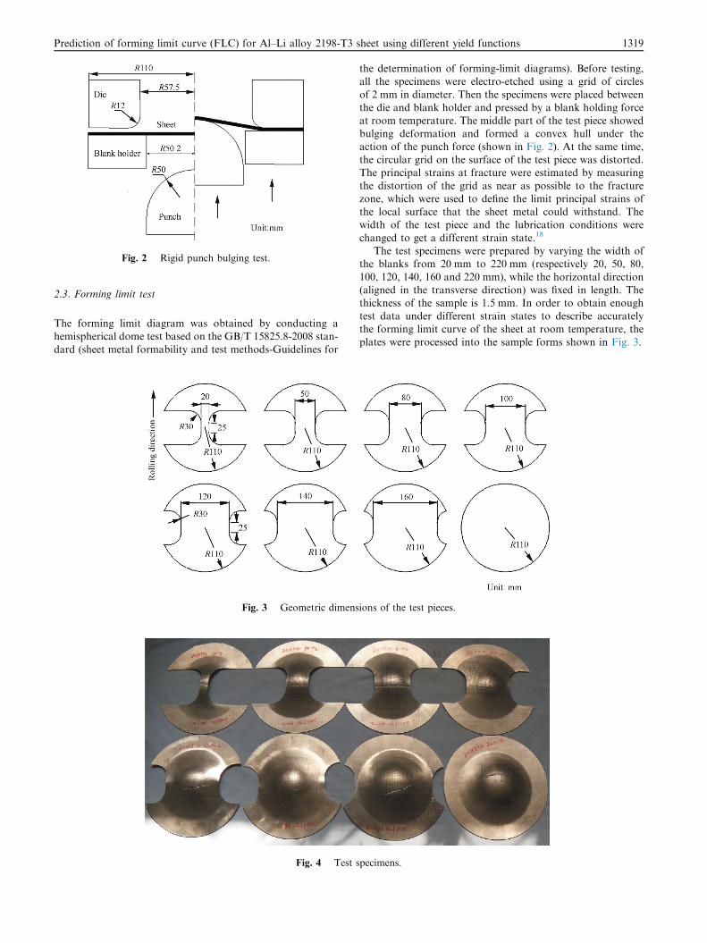
Fig. 2 Rigid punch bulging test.

Prediction of forming limit curve (FLC) for Al–Li alloy 2198-T3 sheet using different yield functions 1319

2.3. Forming limit test

The forming limit diagram was obtained by conducting ahemispherical dome test based on the GB/T 15825.8-2008 stan-

dard (sheet metal formability and test methods-Guidelines for

Fig. 3 Geometric dimens

Fig. 4 Test s

the determination of forming-limit diagrams). Before testing,all the specimens were electro-etched using a grid of circlesof 2 mm in diameter. Then the specimens were placed between

the die and blank holder and pressed by a blank holding forceat room temperature. The middle part of the test piece showedbulging deformation and formed a convex hull under the

action of the punch force (shown in Fig. 2). At the same time,the circular grid on the surface of the test piece was distorted.The principal strains at fracture were estimated by measuring

the distortion of the grid as near as possible to the fracturezone, which were used to define the limit principal strains ofthe local surface that the sheet metal could withstand. Thewidth of the test piece and the lubrication conditions were

changed to get a different strain state.18

The test specimens were prepared by varying the width ofthe blanks from 20 mm to 220 mm (respectively 20, 50, 80,

100, 120, 140, 160 and 220 mm), while the horizontal direction(aligned in the transverse direction) was fixed in length. Thethickness of the sample is 1.5 mm. In order to obtain enough

test data under different strain states to describe accuratelythe forming limit curve of the sheet at room temperature, theplates were processed into the sample forms shown in Fig. 3.

ions of the test pieces.

pecimens.

1320 X. Li et al.

The tested specimens were shown in Fig. 4. The strain ofeach test piece was measured and selected according to thestandards: (1) discard the scattered data point from the three

points in one group if it is far away from the other two closepoints; (2) keep these three points if they are gathered togetheror relatively dispersed in the same coordinate system.19

3. Theoretical prediction of FLC

3.1. M–K theoretical model

The core of the M–K theory is the famous assumption of the

initial inhomogeneity factor: due to geometric or physicalcauses, there is an initial inhomogeneity factor on the directionperpendicular to the direction of the maximum principal stress

when a biaxial tension exists on a sheet metal surface. Thatmeans there is a linear groove before deformation occurs onthe sheet surface. The strain concentration will appear andgrow in the groove with the degree of deformation increasing.

Under this assumption, the localized instability of the sheet isactually caused by the existence of initial surface defects.20

The theoretical model diagram is shown in Fig. 5, in which

part B is the uneven deformation zone which is called thegroove part and part A is the uniform deformation area. tAand tB represent the thicknesses of the part A and part B.

r1and r2 are the major stresses.The core equations of the M–K theory include11,19:(1) The volume of the sheet remains the same along with the

sheet deformation:

de1 þ de2 þ de3 ¼ 0 ð1Þ

where dei is the strain increment, the number i (= 1,2,3) rep-resent the rolling, transverse and thickness direction,respectively.

(2) The principal stresses in the three directions of part Aincrease in proportion:

de1A

e1A¼ de2A

e2A¼ de3A

e3Að2Þ

where eiY is strain of part A or B (the letter Y represent the partA or B), the number i represents the three directions. The deiYis strain increment of part A or B.

The ratio of strains is unchanged through the loadingprocess:

de3A

de2A¼ e3A

e2Að3Þ

(3) The increments of transverse strain (minor strain) arethe same both in part A and part B:

Fig. 5 Mathematical model of the M–K theory.

de2A ¼ de2B ¼ de2 ð4Þ

(4) The force equilibrium condition should be satisfied ateach moment during deformation

r1AtA ¼ r1BtB ð5Þ

where riY is stress, the number i represents the three directions,the letter Y represents the part A or B.

(5) The initial inhomogeneity factor:

f0 ¼tB0tA0

ð6Þ

where tA0 and tB0 is the initial thicknesses of part A and B.

3.2. Theoretical prediction of FLC

When plastic deformation occurs, the strain increases faster inthe groove than outside the groove. Therefore the stress statesinside and outside the grooves are different. If we assume that

the stress state remains constant in part A because of the sta-tionary linear load, the load route of part B changes nonlinear-ly along different levels of the yield surface. The stress stateand stress intensity have to be changed to meet the geometric

coordinate conditions and static equilibrium conditions in or-der to reach the planar strain state, in which the groove deep-ens (de1B > de1A) and the material is thought to lose its ability

to bear the deformation, and then localized necking occurs.The strain increment de1A of part A is given, with which we

can calculate de2A and get the value of de3A with the volume

conditions:

de3 ¼ �ðde1 þ de2Þ ð7Þ

All the strain values change with the increase of the strainincrement as follows:

e ¼ e0 þ de ð8Þ

where e0 is the initial train.The compatibility condition is used to link the two regions

A and B with the algorithm:

ðeA þ deAÞn=uA ¼ f0eðe3B�e3AÞðeB þ deBÞn=uB ð9Þ

where eY is equivalent strain of part A or B (the letter Y repre-sents the part A or B). deY is increment of equivalent strain. rY

is equivalent stress. The process parameter uY is the ratio ofthe equivalent stress and major stress (uY ¼ rY=r1)

3.3. Hardening law formulation

The selection of a material hardening law is essential to theaccuracy of stress calculation from measured strains. Uniaxial

tension tests were performed for getting the stress–straincurves of Al–Li alloy 2198-T3 sheet. The true stress–true straindata measured in the test were fitted to the equation as

follows:21

r ¼ Ken ð10Þ

The hardeningmodel parametersK and n, respectively repre-sent the strength coefficient and strain hardening exponent. The

values ofK and n can be obtained from the fitting calculation ofuniaxial tension test based on the constitutive model equationabove. Fig. 6 is a comparison diagram between the experimen-

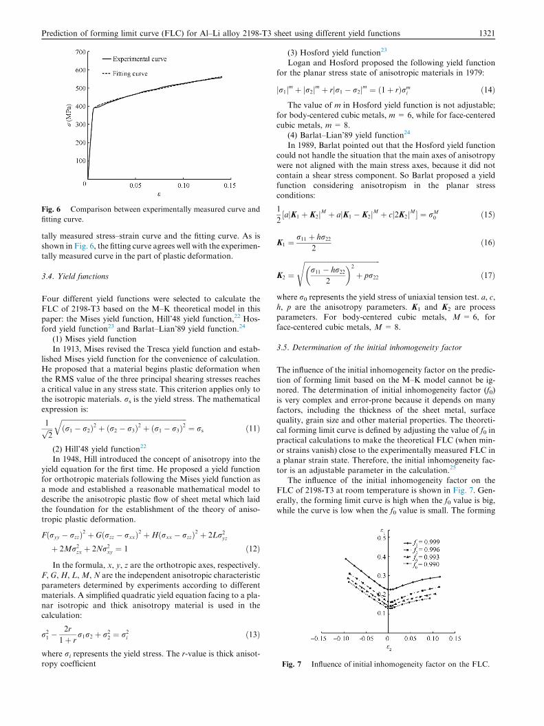
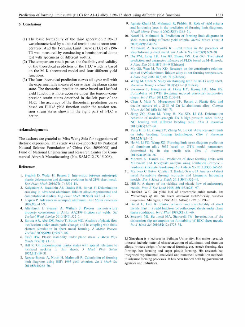
Fig. 7 Influence of initial inhomogeneity factor on the FLC.

Fig. 6 Comparison between experimentally measured curve and

fitting curve.

Prediction of forming limit curve (FLC) for Al–Li alloy 2198-T3 sheet using different yield functions 1321

tally measured stress–strain curve and the fitting curve. As isshown in Fig. 6, the fitting curve agrees well with the experimen-tally measured curve in the part of plastic deformation.

3.4. Yield functions

Four different yield functions were selected to calculate the

FLC of 2198-T3 based on the M–K theoretical model in thispaper: the Mises yield function, Hill’48 yield function,22 Hos-ford yield function23 and Barlat–Lian’89 yield function.24

(1) Mises yield functionIn 1913, Mises revised the Tresca yield function and estab-

lished Mises yield function for the convenience of calculation.He proposed that a material begins plastic deformation when

the RMS value of the three principal shearing stresses reachesa critical value in any stress state. This criterion applies only tothe isotropic materials. rs is the yield stress. The mathematical

expression is:

1ffiffiffi2p

ffiffiffiffiffiffiffiffiffiffiffiffiffiffiffiffiffiffiffiffiffiffiffiffiffiffiffiffiffiffiffiffiffiffiffiffiffiffiffiffiffiffiffiffiffiffiffiffiffiffiffiffiffiffiffiffiffiffiffiffiffiffiffiffiffiffiffiffiffiffiffiffiffiðr1 � r2Þ2 þ ðr2 � r3Þ2 þ ðr1 � r3Þ2

q¼ rs ð11Þ

(2) Hill’48 yield function22

In 1948, Hill introduced the concept of anisotropy into theyield equation for the first time. He proposed a yield function

for orthotropic materials following the Mises yield function asa mode and established a reasonable mathematical model todescribe the anisotropic plastic flow of sheet metal which laid

the foundation for the establishment of the theory of aniso-tropic plastic deformation.

Fðryy � rzzÞ2 þ Gðrzz � rxxÞ2 þHðrxx � rzzÞ2 þ 2Lr2yz

þ 2Mr2zx þ 2Nr2

xy ¼ 1 ð12Þ

In the formula, x, y, z are the orthotropic axes, respectively.

F, G,H, L,M, N are the independent anisotropic characteristicparameters determined by experiments according to differentmaterials. A simplified quadratic yield equation facing to a pla-

nar isotropic and thick anisotropy material is used in thecalculation:

r21 �

2r

1þ rr1r2 þ r2

2 ¼ r2i ð13Þ

where ri represents the yield stress. The r-value is thick anisot-ropy coefficient

(3) Hosford yield function23

Logan and Hosford proposed the following yield functionfor the planar stress state of anisotropic materials in 1979:

jr1jm þ jr2jm þ rjr1 � r2jm ¼ ð1þ rÞrmi ð14Þ

The value of m in Hosford yield function is not adjustable;

for body-centered cubic metals, m= 6, while for face-centeredcubic metals, m= 8.

(4) Barlat–Lian’89 yield function24

In 1989, Barlat pointed out that the Hosford yield functioncould not handle the situation that the main axes of anisotropywere not aligned with the main stress axes, because it did notcontain a shear stress component. So Barlat proposed a yield

function considering anisotropism in the planar stressconditions:

1

2½ajK1 þ K2jM þ ajK1 � K2jM þ cj2K2jM� ¼ rM

0 ð15Þ

K1 ¼r11 þ hr22

2ð16Þ

K2 ¼

ffiffiffiffiffiffiffiffiffiffiffiffiffiffiffiffiffiffiffiffiffiffiffiffiffiffiffiffiffiffiffiffiffiffiffiffiffiffiffiffiffiffiffiffir11 � hr22

2

� �2

þ pr22

sð17Þ

where r0 represents the yield stress of uniaxial tension test. a, c,h, p are the anisotropy parameters. K1 and K2 are processparameters. For body-centered cubic metals, M = 6, for

face-centered cubic metals, M = 8.

3.5. Determination of the initial inhomogeneity factor

The influence of the initial inhomogeneity factor on the predic-tion of forming limit based on the M–K model cannot be ig-nored. The determination of initial inhomogeneity factor (f0)

is very complex and error-prone because it depends on manyfactors, including the thickness of the sheet metal, surfacequality, grain size and other material properties. The theoreti-

cal forming limit curve is defined by adjusting the value of f0 inpractical calculations to make the theoretical FLC (when min-or strains vanish) close to the experimentally measured FLC ina planar strain state. Therefore, the initial inhomogeneity fac-

tor is an adjustable parameter in the calculation.25

The influence of the initial inhomogeneity factor on theFLC of 2198-T3 at room temperature is shown in Fig. 7. Gen-

erally, the forming limit curve is high when the f0 value is big,while the curve is low when the f0 value is small. The forming

Fig. 9 Influence of r-value on the FLC.

1322 X. Li et al.

limit curve drops down with the decrease of value f0 up to aparticular location which corresponds to a constant value of f0.

With reference to the forming limit curve shown in Fig. 7,

the theoretical forming limit curve exhibits good agreementwith the experimentally measured forming limit curve byadjusting the value of f0 when predicting the FLC at room tem-

perature. 0.99 is selected to be the value of the initial inhomo-geneity factor.

3.6. Influence of n-value (hardening exponent)

The hardening exponent is another important parameter witha significant impact on the FLC. Fig. 8 is a comparison of dif-

ferent curves based on different n-values. We can draw a con-clusion that the curve is higher with the increase of the n-value.Due to the fact that the differences of the tested n-valuesshown in Table 2 are not significant, the influence of the

n-value is within an acceptable range. The minimum n-valueis selected in the calculation for safety, because the correspond-ing curve is the lowest.

3.7. Influence of r-value (thick anisotropy coefficient)

The r-value (thick anisotropy coefficient) is the ratio of strains

in the width direction to the thickness direction. Due to the sig-nificant variation of the r-value shown in Table 2, the influenceof the r-value on the FLC should be taken into account. Theforming limit curves based on the same parameters but three

different r-values are calculated and compared in Fig. 9. Wecan conclude that the influence of the r-value on the forminglimit curve can be ignored. The r-value used in the calculation

is the average of the r-values obtained from uniaxial tensiontests in three directions (0�, 45� and 90� directions). (See Eq.(18)). So the theoretical calculation based on the basic form-

ability parameters is credible.

r ¼ ðr0 þ 2r45 þ r90Þ=4 ð18Þ

4. Theoretical prediction of FLC

The theoretical predictions are compared with the forming lim-it data received from the punch bulging test based on the sameparameters in order to verify their feasibility and validity.

Fig. 8 Influence of n-value on the FLC.

Fig. 10 is the comparison diagram between the forming lim-

it curves of experimental data and theoretical prediction atroom temperature. We can draw a conclusion that the experi-mentally measured data points are intensive; at the same time

all the four theoretical prediction curves agree well with theexperimentally measured curve near the planar strain statebut are different from the experimentally measured curve onboth sides of the curve away from the planar strain state.

The experimentally measured data points on the left side aredistributed evenly around the theoretical prediction curvesbased on four different yield functions under the tension–com-

pression strain states. The prediction curve derived from Hos-ford yield function is more accurate, and the anisotropic index(r) has little effect on the FLC. The prediction curves on the

right side are slightly lower than the experimentally measureddata under the tension–tension strain states, and the predictioncurve based on Hill’48 yield function is closer to the experi-mentally measured curve. The prediction of FLC is more accu-

rate when the value of r is greater than 1 due to theapplicability of the Hill’48 yield function. In general, the theo-retical prediction of the FLC shows good agreement with the

measured results, which means the theoretical FLC based onmaterial parameters, different yield functions and M–K theoryis valid.

Fig. 10 Comparison diagram of the measured data and

theoretical prediction curves.

Prediction of forming limit curve (FLC) for Al–Li alloy 2198-T3 sheet using different yield functions 1323

5. Conclusions

(1) The basic formability of the third generation 2198-T3was characterized by a uniaxial tension test at room tem-perature. And the Forming Limit Curve (FLC) of 2198-

T3 was measured by conducting a hemispherical dometest with specimens of different widths.

(2) The comparison result proves the feasibility and validity

of the theoretical prediction of the FLC which is basedon the M–K theoretical model and four different yieldfunctions.

(3) The four theoretical prediction curves all agree well with

the experimentally measured curve near the planar strainstate. The theoretical prediction curve based on Hosfordyield function is more accurate under the tension–com-

pression strain states described in the left part of theFLC. The accuracy of the theoretical prediction curvebased on Hill’48 yield function under the tension–ten-

sion strain states shown in the right part of FLC isbetter.

Acknowledgements

The authors are grateful to Miss Wang Sida for suggestions ofrhetoric expression. This study was co-supported by National

Natural Science Foundation of China (No. 50905008) andFund of National Engineering and Research Center for Com-mercial Aircraft Manufacturing (No. SAMC12-JS-15-008).

References

1. Steglich D, Wafai H, Besson J. Interaction between anisotropic

plastic deformation and damage evolution in Al 2198 sheet metal.

Eng Fract Mech 2010;77(17):3501–18.

2. Kalyanam S, Beaudoin AJ, Dodds RH, Barlat F. Delamination

cracking in advanced aluminum–lithium alloys-experimental and

computational studies. Eng Fract Mech 2009;76(14):2174–91.

3. Lequeu P. Advances in aerospace aluminum. Adv Mater Processes

2008;9(2):47–9.

4. Altenkirch J, Steuwer A, Withers J. Process microstructure

property correlations in Al–Li AA2199 friction stir welds. Sci

Technol Weld Joining 2010;15(6):522–7.

5. Barata AR, Abel DS, Pedro T, Butuc MC. Analysis of plastic flow

localization under strain paths changes and its coupling with finite

element simulation in sheet metal forming. J Mater Process

Technol 2009;209(11):5097–109.

6. Swift HW. Plastic instability under plane stress. J Mech Phys

Solids 1952;1(1):1–18.

7. Hill R. On discontinuous plastic states with special reference to

localized necking in thin sheets. J Mech Phys Solids

1952;1(1):19–31.

8. Rezaee-Bazzaz A, Noori H, Mahmudi R. Calculation of forming

limit diagrams using Hill’s 1993 yield criterion. Int J Mech Sci

2011;53(4):262–70.

9. Aghaie-Khafri M, Mahmudi R, Pishbin H. Role of yield criteria

and hardening laws in the prediction of forming limit diagrams.

Metall Mater Trans A 2002;33(5):1363–71.

10. Noori H, Mahmudi R. Prediction of forming limit diagrams in

sheet metals using different yield criteria. Metall Mater Trans A

2007;38(9):2040–52.

11. Marciniak Z, Kuczynski K. Limit strain in the processes of

stretch-forming sheet metal. Int J Mech Sci 1967;9(9):609–20.

12. Du PM, Lang LH, Liu BS, Zhang DX, Cai GC. Theoretical

prediction and parameter influence of FLDs based on M–K mode.

J Plast Eng 2011;18(5):84–9 [Chinese].

13. Ma GS, Wan M, Wu XD. Research on the constitutive relation-

ship of 5A90 aluminum–lithium alloy at hot forming temperature.

J Plast Eng 2007;14(3):68–71 [Chinese].

14. Wang M, Chen S. Study on stamping limit of Al–Li alloy sheet.

Aeronaut Manuf Technol 2003(5);45–6 [Chinese].

15. Kwansoo C, Kanghwan A, Dong HY, Kyung HC, Min HS.

Formability of TWIP (twinning induced plasticity) automotive

sheets. Int J Plast 2011;27(1):52–81.

16. Chen J, Madi Y, Morgeneyer TF, Besson J. Plastic flow and

ductile rupture of a 2198 Al–Cu–Li aluminum alloy. Comput

Mater Sci 2011;50(4):1365–71.

17. Jiang ZQ, Zhan M, Yang H, Xu XD, Li GJ. Deformation

behavior of medium-strength TA18 high-pressure tubes during

NC bending with different bending radii. Chin J Aeronaut

2011;24(5):657–64.

18. Yang H, Li H, Zhang ZY, Zhang M, Liu GJ. Advances and trends

on tube bending forming technologies. Chin J Aeronaut

2012;25(1):1–12.

19. He M, Li FG, Wang ZG. Forming limit stress diagram prediction

of aluminum alloy 5052 based on GTN model parameters

determined by in situ tensile test. Chin J Aeronaut

2011;24(3):378–86.

20. Morteza N, Daniel EG. Prediction of sheet forming limits with

Marciniak and Kuczynski analysis using combined isotropic –

nonlinear kinematic hardening. Int J Mech Sci 2011;53(2):145–53.

21. Marilena C. Butuc, Cristian T, Barlat, Gracio JJ. Analysis of sheet

metal formability through isotropic and kinematic hardening

models. Eur J Mech A Solids 2011;30(4):532–46.

22. Hill R. A theory of the yielding and plastic flow of anisotropic

metals. Proc R Soc Lond 1948;193(1033):281–97.

23. Hosford WF, On yield loci of anisotropic cubic metals. In:

Proceedings of the 7th north american metalworking research

conference. Michigan, USA: Ann Arbor; 1979. p. 191–7.

24. Barlat F, Lian K. Plastic behavior and stretchability of sheet

metals. Part I: a yield function for orthotropic sheets under plane

stress conditions. Int J Plast 1989;5(1):51–66.

25. Serenelli MJ, Bertinetti MA, Signorelli JW. Investigation of the

dislocation slip assumption on formability of BCC sheet metals.

Int J Mech Sci 2010;52(12):1723–34.

Li Xiaoqiang is a lecturer in Beihang University. His major research

interests include material characterization of aluminum and titanium

alloys, process design of sheet metal forming, e.g. stretch forming, flex

forming, hot forming and super plastic forming. His research has

integrated experimental, analytical and numerical simulation methods

to advance forming processes. It has been funded both by government

agencies and industries.