Computational analysis of the importance of flow synchronyfor cardiac ventricular assist devices

Matthew McCormick a, David Nordsletten b, Pablo Lamata b, Nicolas P. Smith a,b,c,n

a Department of Computer Science, University of Oxford, Wolfson Building, Parks Road, OX1 3QD, UKb Department of Biomedical Engineering, King's College London, The Rayne Institute, 4th Floor Lambeth Wing, St Thomas' Hospital, SE1 7EH, UKc Faculty of Engineering, University of Auckland, 20 Symonds St, Auckland, New Zealand

a r t i c l e i n f o

Article history:Received 18 November 2013Accepted 28 March 2014

Keywords:Fluid–structureComputational modelCardiovascularTissue mechanicsComputer model

a b s t r a c t

This paper presents a patient customised fluid–solid mechanics model of the left ventricle (LV)supported by a left ventricular assist device (LVAD). Six simulations were conducted across a range ofLVAD flow protocols (constant flow, sinusoidal in-sync and sinusoidal counter-sync with respect to thecardiac cycle) at two different LVAD flow rates selected so that the aortic valve would either open(60 mL s�1) or remain shut (80 mL s�1). The simulation results indicate that varying LVAD flow in-syncwith the cardiac cycle improves both myocardial unloading and the residence times of blood in the leftventricle. In the simulations, increasing LVAD flow during myocardial contraction and decreasing itduring diastole improved the mixing of blood in the LV cavity. Additionally, this flow protocol had theeffect of partly homogenising work across the myocardium when the aortic valve did not open, reducingmyocardial stress and thereby improving unloading.

& 2014 Elsevier Ltd. All rights reserved.

1. Introduction

Heart failure is the leading cause of hospitalisation among olderadults in Western society with a lifetime risk of 20% at age 40.Despite improved medical and surgical techniques, mortality afterthe onset of heart failure remains high, ranging from 20 to 50% [6].Orthotropic heart transplantation is recognised as the best therapyfor end-stage heart failure [26]. However, approximately 20 to 30%of potential recipients die while waiting for a donor heart [29].Due to this shortage, left ventricular assist devices (LVADs) areoften used as a bridge to transplant [1].

The role of these LVAD pumps is to reduce the mechanical loadon the heart by pumping blood from the left ventricular (LV)apex directly to the aorta, with the implantation of these devicessignificantly reducing both LV pressure and volume [9]. Postimplantation, it is standard practice for clinicians to tune LVADflow so that the aortic valve opens occasionally to prevent it fusingshut [27]. However, the impact of valve opening on myocardialunloading and the residence times of blood within the ventricleremains unknown. Both these factors are of critical importancewith respect to improving treatment outcome for patients – too

much unloading can lead to myocardial atrophy, while too littleresults in the myocardium remaining over-stressed [14]. A furtherconsideration is the impact of LVAD flow on blood residence times,where inadequate recirculation has the potential to increase therisk of thrombosis formation [2]. Tuning the device to optimise forthese factors involves varying both LVAD flow rate and LVAD flowsynchrony – i.e. whether the LVAD cannula outflow is constant orvaries through the cardiac cycle. However, these parameters resultin substantial variation in cardiac behaviour, ranging from deter-mining whether the aortic valve opens at all, through to the extentto which LV volume changes through the cardiac cycle.

A central difficulty for this type of optimisation is the challengeof observing cardiac function and cardiovascular flows under LVADsupport using standard medical image modalities, such as MRI andechocardiography, due to the positioning of the pump, along withits metallic components. This context motivates the applicationof mathematical modelling techniques as an investigative tool forstudying the behaviour of the ventricle under LVAD support andanalysing its efficacy as a pump. For such analyses to facilitatethe optimisation of LVAD support, the interaction at the core ofventricular function needs to be addressed – i.e. the couplingbetween blood flow in the ventricular chamber and the myocar-dium. As a result, coupled fluid–solid mechanical models arerequired with the ability to support investigations into the impactof LVAD support on ventricular hemodynamics and myocardialmechanics.

Contents lists available at ScienceDirect

journal homepage: www.elsevier.com/locate/cbm

Computers in Biology and Medicine

http://dx.doi.org/10.1016/j.compbiomed.2014.03.0130010-4825/& 2014 Elsevier Ltd. All rights reserved.

n Corresponding author at: Faculty of Engineering, University of Auckland, 20Symonds St, Auckland, New Zealand.

E-mail address: np.smith@auckland.ac.nz (N.P. Smith).

Computers in Biology and Medicine 49 (2014) 83–94

Several coupled fluid–solid mechanical LV models currentlyexist in the literature, ranging from the pioneering work ofMcQueen and Peskin [17,25] through to recent models incorpor-ating greater degrees of physical realism, in particular, in thedescription of myocardial behaviour [22]. These models have beenused to investigate blood flow within the ventricular cavities andthe efficiency of the heart as a pump from diastole [3] through tosystole [11,22,32,33]. Recently, we [15,16] have extended a non-conforming finite element fluid–solid mechanics scheme [21] tofacilitate the simulation of LVAD supported LVs through thefull cardiac cycle. Using a fictitious domain (FD) [31] method toprescribe the LVAD cannula, the application of this approachenables the interaction between the cannula and the myocardialwall to be captured, facilitating the simulation of the full range ofcardiac behaviour.

In this study we apply this framework for the first time to apatient customised geometry to present the first (to our knowl-edge) numerical investigation into the impact of aortic valveopening and LVAD flow synchrony on ventricular hemodynamicsand myocardial mechanics. Specifically, the developed model isapplied to investigate the mixing of blood within the LV chamber,as well as the efficiency of myocardial work transduction underdifferent LVAD flow protocols.

2. Materials and methods

2.1. Model framework

Derived from the principles of conservation of mass andmomentum, and as outlined in detail in our previous publications[16,22], we have developed a model that provides a physiologicaldescription of the myocardium and ventricular blood flow. In brief,the model was solved using a non-conforming Galerkin finiteelement scheme to enable varying degrees of refinement toadequately resolve the blood and myocardial spatial domains. Thisscheme enables high levels of physiological detail (including thecomplex fibre architecture [13] and biophysically based constitu-tive laws) to be incorporated.

To resolve the physical system, ventricular blood flow and myo-cardial mechanics were modelled using the arbitrary Lagrange–Eulerian form of the Navier–Stokes equations [20] and thequasi-static finite elasticity equations [23], respectively. To enforcecontinuity between the solid myocardial wall and the fluidventricular chamber, velocities were equated over their commoninterface [21]. This constraint was applied by introducing aLagrange multiplier to enforce equal, but opposite, tractions acrossthe endocardial boundary. To incorporate the LVAD cannula intothe model, a zero velocity boundary condition was implementedon the cannula wall using the fictitious domain method whereby asecond Lagrange multiplier was applied to the FEM weakform.This method enables the cannula boundary to move throughthe fluid domain, resolving the numerical issues resulting fromthe deformation of the fluid mesh [15]. Additionally, it hasbeen demonstrated that application of the fictitious domain termsyields adherence to the velocity constraint weakly [30,31], and themethod is applied to many cardiovascular applications. Further-more, the combination of the two Lagrange multipliers implicitlyresolves the contact problem of an immersed rigid body in adeformable chamber. As a result the model system is capable ofresolving the complete range of cardiac motion – including contactbetween the myocardium and the LVAD cannula [15].

Solving the fluid–solid mechanical model through a wholecycle requires the addition of accurate systemic constraints onthe flow model. This was achieved by integrating the 3D FSI modelwith a 0D Windkessel representation of systemic circulation. In

this work, we coupled the Shi and Korakianitis 0D Windkesselmodel [28] using a fixed point prescribed flow rate technique [16].Using this technique, flow was prescribed according to the pressuregradient across the valve using Bernoulli's equation for the con-servation of energy along the same streamline. Valve opening wasprescribed to occur when LV lumen pressure exceeds aortic sinuspressure. To approximate opening and closing in the 3D model, thevalves were defined as functions on the mitral and aortic bound-aries, with the radius of the open valve assumed to be proportionalto flow rate. The proportionality constant was fitted to matchobserved human data, E 46 ms and E 24 ms for the mitral [34]and aortic [24] valves respectively, see Appendix A for details.

To capture the mechanical properties of the myocardium, thefinite elasticity stress tensor was defined as a combination ofpassive and active components. The stress further incorporatedinformation about myocardial structure, by the introduction of anorthonormal fiber tensor, to denote the fibre, sheet and normaldirections of the tissue [7,19]. In this paper, the passive constitu-tive law was defined using a modified form of the Costa consti-tutive law [4] based on the strain energy functions W and Wiso,where W represents the Costa constitutive contribution and anisotropic stiffness component (see [22] for details of the incor-poration of this component). Additionally, to approximate theinteraction between the cannula base and the myocardium, themyocardial wall was assumed to be stiffer at the junction betweenthe LVAD cannula base and the myocardial wall. Active contractionin the tissue was generated using the Niederer contraction model[18] chosen due to the limited number of parameters enablinga more unique fit to patient data [18]. This 6 parameter modelcaptures the length dependent rates of tension development,along with peak tension.

2.2. Patient model

This framework was applied to a patient specific LV geometrywhich was constructed based on 422 short axis CT image slices takenat end diastole from a 53 year old heart failure patient withan implanted LVAD, all data was acquired as part of a local ethicscommittee at the German Heart Centre approved protocol consistentwith the principles expressed in the Declaration of Helsinki andinformed consent was obtained from the patient. The spatial resolu-tion of the image stack was 0.4 mm�0.4 mm, in the CT image plane,and 0.6 mm in the through plane direction. Digitisation of the imagedata was performed by Phillips Research and the resulting binarysegmentation was used to construct the geometric myocardial mesh.Fig. 1 highlights each stage of the mesh generation procedure. A cubicLagrange myocardial mesh was constructed from an ellipsoidaltemplate using an automated meshing tool that implements theprocedure previously outlined [12]. Mean error from the fittingprocedure (with respect to the normal distance between binary dataand the fitted mesh) was 0.7271.05 mm. The final fitted cubicLagrange mesh was interpolated from the warped cubic Hermitegeometry. The resulting cubic hexahedral mesh consisted of 324elements, with a through wall thickness of 3 elements. An idealisedfibre geometry, 7601 with respect to the endo/epicardial surfaces,was defined within the myocardial geometry.

Within the ventricular cavity a linear tetrahedral fluid mesh,consisting of � 3:2� 104 elements, was constructed using thesoftware package CUBIT,1 with a characteristic mesh length of3.2 mm. The linear mesh was modified to provide a curvilineardescription (quadratic Crouzeix–Raviart [5] elements) of the cavityby projecting surface nodes onto the endocardial surface. Internalnodes were unchanged maintaining the linear spatial description

1 http://cubit.sandia.gov.

M. McCormick et al. / Computers in Biology and Medicine 49 (2014) 83–9484

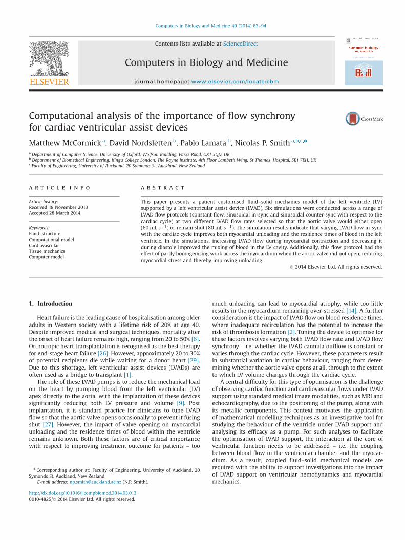
of non-boundary fluid elements. The LVAD cannula introduced bythe fictitious domain approach was incorporated using the geo-metry provided by Berlin Heart. The boundary mesh was con-structed, with a characteristic length equivalent to that of the fluidmesh, from 544 linear triangular elements.

2.2.1. Experimental protocolSimulations on the patient model were performed using a

variety of LVAD flow protocols, ranging from constant LVAD flowrates at 60 and 80 mL s�1, to flow varying sinusoidally – thoughalways positive – through the cardiac cycle (either increasing ordecreasing during systole) with mean flow rates of 60 and80 mL s�1. The protocols, defined in Table 1, were selected to testthe impact of both aortic valve opening2 (with a mean flow rate of60 mL s�1 the valve opened while at 80 mL s�1 it remained shut)and whether increasing or decreasing LVAD outflow during systoleimpacted myocardial unloading or the residence times of bloodwithin the ventricular chamber.

For each flow protocol, simulations were performed for twoheart beats, each of one second, consisting of 2500 time steps perbeat, with a time step of 0.00025 s during the contractile phasesand 0.001 s during diastole. A linear activation sequence,

endocardium to epicardium, was defined with a period of 0.05 s.The resulting simulations, initiated from end diastole, consisted of� 5:5� 105

fluid and � 3:4� 104 solid degrees of freedom. Thesame external model parameters (i.e. Windkessel and contractionmodels) were used in all cases. All simulations converged onrepeating pressure volume loops, see Fig. 3.

2.2.2. Passive and active myocardial parameter fittingTo incorporate the residual strain, present in the myocardium

at end diastole, a zero-stress, or reference state of the myocardiumwas estimated using the methods previously outlined [15,22].

Fig. 1. Myocardial geometry fitting to patient image data. Top left, digitised binary myocardial map superimposed against a CT slice, LVAD cannula visible; top right, the fittedmyocardial geometry compared with the binary myocardial map; bottom left, the fitted myocardial geometry superimposed against a CT slice; and bottom right,visualisation of the 7601 fibre geometry.

Table 1LVAD flow protocols for the patient study. Time t¼0 was taken with respect to thestart of isovolumetric contraction. In sync refers to increasing LVAD flow duringsystole while counter sync refers to decreasing flow. Total flow rate through onecardiac cycle in the sinusoidal LVAD protocols was the same as for their equivalentconstant flow rate cases.

Simulation Flow rate (mL s�1) Description

L60 QLVAD ¼ 60 Constant flow rateL80 QLVAD ¼ 80 Constant flow rateLs60þ QLVAD ¼ 60þ45 sin ð2πtÞ Sinusoidal flow rate, in syncLs60� QLVAD ¼ 60�45 sin ð2πtÞ Sinusoidal flow rate, counter syncLs80þ QLVAD ¼ 80þ60 sin ð2πtÞ Sinusoidal flow rate, in syncLs80� QLVAD ¼ 80�60 sin ð2πtÞ Sinusoidal flow rate, counter sync

2 Model valves were defined as functions on the mitral and aortic fluidboundaries, Γmi and Γao. Full description of these functions are provided in [15,22].

M. McCormick et al. / Computers in Biology and Medicine 49 (2014) 83–94 85

Here, the Costa constitutive parameters were fitted to the Klotzpressure volume relationship [10] defined by the end diastolicvolume of 240.95 mL and pressure of 13.13 mmHg. Since patientspecific pressure data was not available, the pressure valuewas taken from equivalent LVAD supported patient data [9]. Thecontraction parameters were tuned so that LV stroke volume wasE 50 mL and peak systolic pressure was between 100 and120 mmHg when the LVAD was switched off. This was consistentwith observations [9]. Additionally, due to the slow rate of myo-cardial relaxation typically observed in cardiomyopic heart failurepatients [8], the desired durations of isovolumetric contraction andrelaxation were 0.1 s and 0.2 s, with a systolic period of 0.2 s.

The pressure volume relationships from the iterative updates ofthe passive fitting procedure (along with the ideal Klotz relation-ship) are shown in Fig. 2, along with a sampling of PV relationshipsfrom a set of simulations solving only the solid problem across arange of parameters. The final fitted parameters are provided inTables 2 and 3.

2.2.3. Initial and boundary conditionsSolid only simulations were performed to converge the myo-

cardial and Windkessel models on repeating pressure volumeloops for each of the flow protocols. The solutions from eachof these simulations were used as the initial conditions for theirrespective fluid–solid coupled simulations. Due to differences inafterload in the 60 and 80 ml s�1 cases, initial end-diastolicvolumes were 5–10% lower in the 80 ml cases. The relevant LVand Windkessel model initial conditions are provided in Table 4.Note that due to continuous flow through the LVAD, increasedLVAD flow rates led to increased aortic pressures.

3. Results

In both the L60 and L80 cases, increasing LVAD outflow duringsystole and reducing it during diastole increased the range of LVvolumes through the cardiac cycle and reduced peak LV pressure.The opposite effect was observed when LVAD outflow decreasedduring systole. Comparing the L60 and L80 cases, LV volume wassignificantly lower in the L80 cases, while peak LV pressures werelower in all equivalent L80 simulations (see Fig. 3). Additionally, therange in LV volume was greatest in the Ls80þ case and smallest inthe Ls80� case.

It is thus convenient, particularly given that systole does notnecessarily occur in supported hearts at high LVAD flow rates, to

consider two broad periods of cardiac behaviour, the contractilephases (i.e. IVC, systole and IVR) and diastole. Using this distinc-tion to divide the results, the blood flow streamlines and myo-cardial displacements from selected time points during the secondheart beat in the L60 cases are shown in Fig. 4, while theendocardial fluid pressures at the same time points are presentedin Fig. 5. With the exception of the 0.21 s time point where theaortic outflow was not observed, the flow profiles in the L80 caseswere similar to those observed in Fig. 4.

At the opening of the aortic valve (0.21 s), significant flow inthe direction of the valve was produced, however, due to theweakness of aortic flow as a result of continued LVAD outflow,sustained helical features were observed at the far wall from the

Fig. 2. Fitting of patient passive myocardial parameters. Left, iterative updates of the passive PV relationship (iteration 1–4), fitted for an end diastolic volume and pressure of240.95 mL and 13.13 mmHg respectively. Red shows the reference Klotz relationship; Right, a sample of PV loops from the fitting of the active tension and Windkesselmodels. The models were fitted for a stroke volume of � 50 mL s�1 and peak LV pressure during systole of between 100 and 120 mmHg. The final fitted relationship is in red.(For interpretation of the references to colour in this figure caption, the reader is referred to the web version of this article.)

Table 2Fitted Costa law parameters for the patient myocardial model. Note αij issymmetric.

C(KPa) α1;1 α2;2 α3;3 α1;2 α1;3 α2;3 α0 Cϕ

380.05 33.41 6.45 3.61 14.68 10.92 4.83 33.41 3000

Table 3Fitted parameters for the Niederer contraction model.

T0 (KPa) tr0 td a1 a2 a3

120 0.11 s 0.199 s 2.0 0.7 3.2

Table 4Initial LV pressures and volumes, as well as the Windkessel model initial values forthe left atria (LA) and aorta (Ao). The values were taken from the solid only modelsat end diastole, after convergence on a repeating pressure volume loop. Pressures(P) are given in mmHg, while volumes (V) are in mL. All initial flow rates across themitral and aortic valves, as well as the LVAD cannula, were zero.

Simulation LV parameters Windkessel parameters

VLV PLV PLA VLA PAo

L60 232.37 10.60 9.79 42.49 107.49L80 225.55 8.75 8.35 36.19 120.18Ls60þ 234.38 11.21 10.23 44.41 101.74Ls60� 230.01 9.92 9.30 40.33 113.56Ls80þ 227.79 9.32 8.74 37.90 114.22Ls80� 222.35 7.99 7.82 33.87 126.80

M. McCormick et al. / Computers in Biology and Medicine 49 (2014) 83–9486

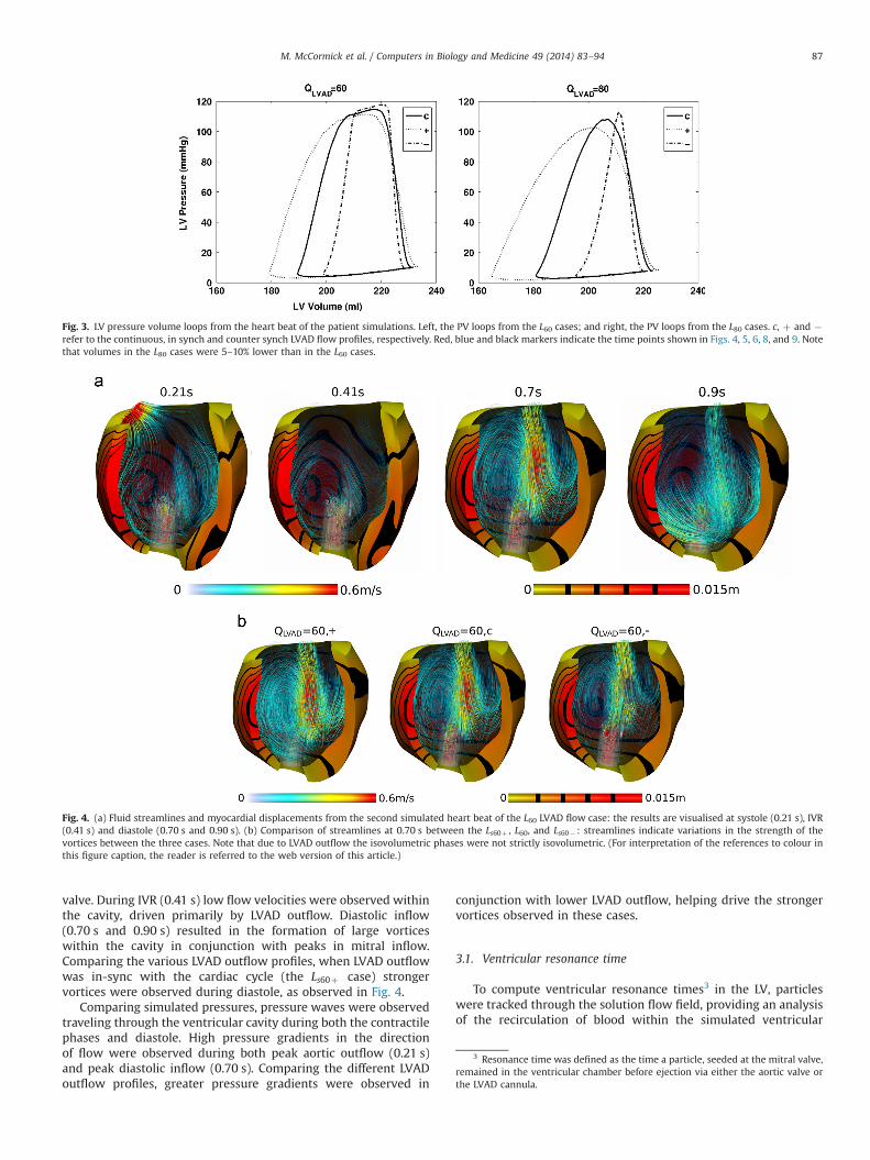
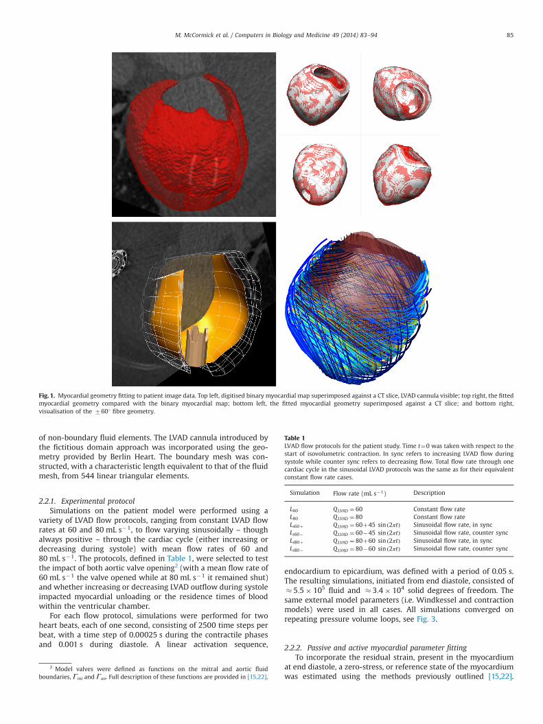
valve. During IVR (0.41 s) low flow velocities were observed withinthe cavity, driven primarily by LVAD outflow. Diastolic inflow(0.70 s and 0.90 s) resulted in the formation of large vorticeswithin the cavity in conjunction with peaks in mitral inflow.Comparing the various LVAD outflow profiles, when LVAD outflowwas in-sync with the cardiac cycle (the Ls60þ case) strongervortices were observed during diastole, as observed in Fig. 4.

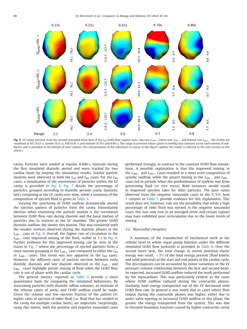
Comparing simulated pressures, pressure waves were observedtraveling through the ventricular cavity during both the contractilephases and diastole. High pressure gradients in the directionof flow were observed during both peak aortic outflow (0.21 s)and peak diastolic inflow (0.70 s). Comparing the different LVADoutflow profiles, greater pressure gradients were observed in

conjunction with lower LVAD outflow, helping drive the strongervortices observed in these cases.

3.1. Ventricular resonance time

To compute ventricular resonance times3 in the LV, particleswere tracked through the solution flow field, providing an analysisof the recirculation of blood within the simulated ventricular

Fig. 3. LV pressure volume loops from the heart beat of the patient simulations. Left, the PV loops from the L60 cases; and right, the PV loops from the L80 cases. c, þ and �refer to the continuous, in synch and counter synch LVAD flow profiles, respectively. Red, blue and black markers indicate the time points shown in Figs. 4, 5, 6, 8, and 9. Notethat volumes in the L80 cases were 5–10% lower than in the L60 cases.

Fig. 4. (a) Fluid streamlines and myocardial displacements from the second simulated heart beat of the L60 LVAD flow case: the results are visualised at systole (0.21 s), IVR(0.41 s) and diastole (0.70 s and 0.90 s). (b) Comparison of streamlines at 0.70 s between the Ls60þ , L60, and Ls60� : streamlines indicate variations in the strength of thevortices between the three cases. Note that due to LVAD outflow the isovolumetric phases were not strictly isovolumetric. (For interpretation of the references to colour inthis figure caption, the reader is referred to the web version of this article.)

3 Resonance time was defined as the time a particle, seeded at the mitral valve,remained in the ventricular chamber before ejection via either the aortic valve orthe LVAD cannula.

M. McCormick et al. / Computers in Biology and Medicine 49 (2014) 83–94 87

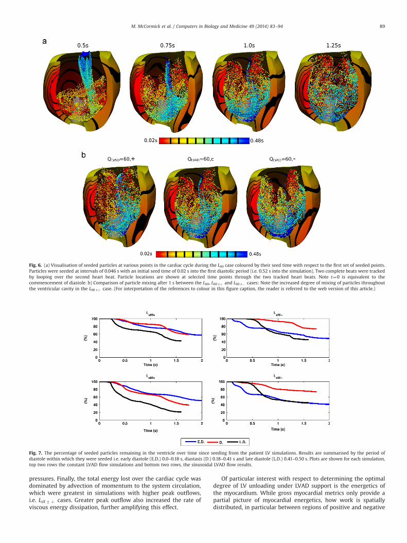
cavity. Particles were seeded at regular, 0.046 s, intervals duringthe first simulated diastolic period and were tracked for twocardiac beats by looping the simulation results. Similar particlemotions were observed in both the L60 and L80 cases. For the L60cases, a visualisation of the movements of particles within the LVcavity is provided in Fig. 6. Fig. 7 details the percentage ofparticles, grouped according to diastolic periods (early, diastasis,late), remaining in the LV cavity over time, while a summary of thecomposition of ejected fluid is given in Table 5.

Varying the synchrony of LVAD outflow dramatically alteredthe ejection pattern of particles from the cavity. Immediatelyobvious when examining the particle motion is the correlationbetween LVAD flow rate during diastole and the basal motion ofparticles due to vortices in the LV chamber. The greater LVADdiastolic outflow, the slower this motion. This was consistent withthe weaker vortices observed during the diastolic phases in theLs60� case in Fig. 4. Overall, the higher rate of circulation in theLs60þ case improved mixing of the fluid, visible at 1 s in Fig. 6.Further evidence for this improved mixing can be seen in thetraces in Fig. 7 where the percentage of ejected particles form amore narrow grouping in the Ls60þ case compared to either the L60or Ls60� cases. This trend was less apparent in the L80 cases.However, the different rates of particle ejection between earlydiastole, diastasis and late diastole observed in the Ls60� andLs80� cases highlight poorer mixing of fluid when the LVAD flowrate is out of phase with the cardiac cycle.

The general metrics reported in Table 5 provide a morequantitative basis for comparing the simulated behaviours. Byassociating particles with diastolic inflow volumes, an estimate ofthe volume ratios of aortic and LVAD outflow could be made.Given the volume and low ejection fraction of the patient LV,higher rates of ejection of older fluid (i.e. fluid that has resided inthe cavity for multiple cardiac beats) are important. Surprisingly,using this metric, both the positive and negative sinusoidal cases

performed strongly, in contrast to the constant LVAD flow simula-tions. A possible explanation is that the improved mixing inthe Ls60þ and Ls80þ cases resulted in a more even composition ofsystolic outflow, while the poorer mixing in the Ls60� and Ls80�cases led to periods when the predominance of outflow was frompreexisting fluid (or vice versa). Both instances would resultin improved ejection rates for older particles. The poor ratiosobserved from the negative sinusoidal cases in the % S.V. beat1 column in Table 5 provide evidence for this explanation. Thisresult does not, however, rule out the possibility that while a highpercentage of older fluid was ejected in the negative sinusoidalcases, this was only true in an averaged sense and certain regionsmay have exhibited poor recirculation due to the lower levels ofmixing.

3.2. Myocardial energetics

A summary of the transduction of mechanical work at thecellular level to whole organ pump function under the differentsimulated LVAD flow protocols is provided in Table 6. Over thesecond heart beat, the total change in stored potential elasticenergy was small, o5% of the total energy present (fluid kineticand solid potential) at the start and end points of the cardiac cycle.The discrepancies can be accounted by minor variations in the LVpressure–volume relationship between the first and second beats.As expected, increased LVAD outflow reduced the work performedby the myocardium. This was particularly evident in the caseswhere LVAD outflow reduced during the contractile phases.Similarly, total energy transported out of the LV decreased withLVAD flow rate. In general it was noted that in cases where flowoutput during the contractile phases was higher, either due toaortic valve opening or increased LVAD outflow in this phase, thegreater the energy transported from the system. This was dueto elevated boundary tractions caused by higher contractile cavity

Fig. 5. LV cavity pressure from the second simulated heart beat of the L60 LVAD flow regime cases: top row, Ls60þ , centre row, Ls60þ , and bottom row Ls60� . The results arevisualised at IVC (0.12 s), systole (0.21 s), IVR (0.41 s) and diastole (0.70 s and 0:90 s). The range in pressure values (given in mmHg) was constant across each column of sub-figures and is provided at the bottom of each column. (For interpretation of the references to colour in this figure caption, the reader is referred to the web version of thisarticle.)

M. McCormick et al. / Computers in Biology and Medicine 49 (2014) 83–9488

pressures. Finally, the total energy lost over the cardiac cycle wasdominated by advection of momentum to the system circulation,which were greatest in simulations with higher peak outflows,i.e. LsX7 þ cases. Greater peak outflow also increased the rate ofviscous energy dissipation, further amplifying this effect.

Of particular interest with respect to determining the optimaldegree of LV unloading under LVAD support is the energetics ofthe myocardium. While gross myocardial metrics only provide apartial picture of myocardial energetics, how work is spatiallydistributed, in particular between regions of positive and negative

Fig. 6. (a) Visualisation of seeded particles at various points in the cardiac cycle during the L60 case coloured by their seed time with respect to the first set of seeded points.Particles were seeded at intervals of 0.046 s with an initial seed time of 0.02 s into the first diastolic period (i.e. 0.52 s into the simulation). Two complete beats were trackedby looping over the second heart beat. Particle locations are shown at selected time points through the two tracked heart beats. Note t¼0 is equivalent to thecommencement of diastole. b) Comparison of particle mixing after 1 s between the L60, L60 sþ and L60 s� cases: Note the increased degree of mixing of particles throughoutthe ventricular cavity in the L60 sþ case. (For interpretation of the references to colour in this figure caption, the reader is referred to the web version of this article.)

Fig. 7. The percentage of seeded particles remaining in the ventricle over time since seeding from the patient LV simulations. Results are summarised by the period ofdiastole within which they were seeded i.e. early diastole (E.D.) 0.0–0.18 s, diastasis (D.) 0.18–0.41 s and late diastole (L.D.) 0.41–0.50 s. Plots are shown for each simulation,top two rows the constant LVAD flow simulations and bottom two rows, the sinusoidal LVAD flow results.

M. McCormick et al. / Computers in Biology and Medicine 49 (2014) 83–94 89

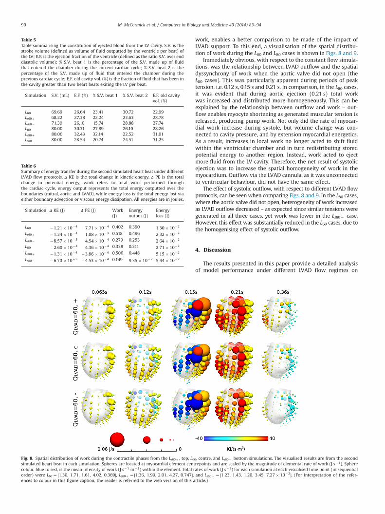
work, enables a better comparison to be made of the impact ofLVAD support. To this end, a visualisation of the spatial distribu-tion of work during the L60 and L80 cases is shown in Figs. 8 and 9.

Immediately obvious, with respect to the constant flow simula-tions, was the relationship between LVAD outflow and the spatialdyssynchrony of work when the aortic valve did not open (theL80 cases). This was particularly apparent during periods of peaktension, i.e. 0.12 s, 0.15 s and 0.21 s. In comparison, in the L60 cases,it was evident that during aortic ejection (0.21 s) total workwas increased and distributed more homogeneously. This can beexplained by the relationship between outflow and work – out-flow enables myocyte shortening as generated muscular tension isreleased, producing pump work. Not only did the rate of myocar-dial work increase during systole, but volume change was con-nected to cavity pressure, and by extension myocardial energetics.As a result, increases in local work no longer acted to shift fluidwithin the ventricular chamber and in turn redistributing storedpotential energy to another region. Instead, work acted to ejectmore fluid from the LV cavity. Therefore, the net result of systolicejection was to increase the spatial homogeneity of work in themyocardium. Outflow via the LVAD cannula, as it was unconnectedto ventricular behaviour, did not have the same effect.

The effect of systolic outflow, with respect to different LVAD flowprotocols, can be seenwhen comparing Figs. 8 and 9. In the L80 cases,where the aortic valve did not open, heterogeneity of work increasedas LVAD outflow decreased – as expected since similar tensions weregenerated in all three cases, yet work was lower in the Ls80� case.However, this effect was substantially reduced in the L60 cases, due tothe homogenising effect of systolic outflow.

4. Discussion

The results presented in this paper provide a detailed analysisof model performance under different LVAD flow regimes on

Table 5Table summarising the constitution of ejected blood from the LV cavity. S.V. is thestroke volume (defined as volume of fluid outputted by the ventricle per beat) ofthe LV; E.F. is the ejection fraction of the ventricle (defined as the ratio S.V. over enddiastolic volume); % S.V. beat 1 is the percentage of the S.V. made up of fluidthat entered the chamber during the current cardiac cycle; % S.V. beat 2 is thepercentage of the S.V. made up of fluid that entered the chamber during theprevious cardiac cycle; E.F. old cavity vol. (%) is the fraction of fluid that has been inthe cavity greater than two heart beats exiting the LV per beat.

Simulation S.V. (mL) E.F. (%) % S.V. beat 1 % S.V. beat 2 E.F. old cavityvol. (%)

L60 69.69 26.64 23.41 30.72 22.99Ls60þ 68.22 27.38 22.24 23.63 28.78Ls60� 71.39 26.10 15.74 28.88 27.74L80 80.00 30.31 27.89 26.10 28.26Ls80þ 80.00 32.43 32.14 22.52 31.01Ls80� 80.00 28.54 20.74 24.51 31.25

Table 6Summary of energy transfer during the second simulated heart beat under differentLVAD flow protocols. Δ KE is the total change in kinetic energy, Δ PE is the totalchange in potential energy, work refers to total work performed throughthe cardiac cycle, energy output represents the total energy outputted over theboundaries (mitral, aortic and LVAD), while energy loss is the total energy lost viaeither boundary advection or viscous energy dissipation. All energies are in Joules.

Simulation Δ KE (J) Δ PE (J) Work(J)

Energyoutput (J)

Energyloss (J)

L60 �1:21� 10�4 7:71� 10�4 0.402 0:390 1:30� 10�2

Ls60þ �1:34� 10�4 1:08� 10�3 0.518 0:496 2:32� 10�2

Ls60� �8:57� 10�5 4:54� 10�4 0.279 0:253 2:64� 10�2

L80 2:60� 10�4 4:36� 10�4 0.338 0.311 2:71� 10�2

Ls80þ �1:31� 10�4 �3:86� 10�4 0.500 0:448 5:15� 10�2

Ls80� �6:70� 10�5 �4:53� 10�4 0.149 9:35� 10�2 5:44� 10�2

Fig. 8. Spatial distribution of work during the contractile phases from the Ls60þ , top, L60, centre, and Ls60� bottom simulations. The visualised results are from the secondsimulated heart beat in each simulation. Spheres are located at myocardial element centrepoints and are scaled by the magnitude of elemental rate of work (J s�1). Spherecolour, blue to red, is the mean intensity of work (J s�1 m�3) within the element. Total rates of work (J s�1) for each simulation at each visualised time point (in sequentialorder) were L60 ¼ ½1:30; 1:71; 1:61; 4:02; 0:369�, Ls60þ ¼ ½1:36; 1:99; 2:01; 4:27; 0:747�, and Ls60� ¼ ½1:23; 1:43; 1:20; 3:45; 7:27� 10�2�. (For interpretation of the refer-ences to colour in this figure caption, the reader is referred to the web version of this article.)

M. McCormick et al. / Computers in Biology and Medicine 49 (2014) 83–9490

a patient LV geometry. Significant variations in hemodynamic andmyocardial dynamics were observed across a range of loadingconditions investigated and these results provide an insight intohow LVAD support impacts gross LV function. This section dis-cusses the conclusions that can be drawn from these simulations,taking into account the impact of model limitations on theseconclusions.

4.1. Particle tracking

A significant observation from particle tracking results was thatthe rate of fluid mixing was correlated with lower LVAD outflowduring diastole. A possible explanation for this result relates to theincrease in mitral inflow during diastasis in cases where LVADoutflow was higher. During diastole, incoming fluid displaces pre-existing fluid at the LV apex, forcing this volume towards the LVbase. At lower diastolic LVAD flow rates, this displacement inducedthe formation of vortices that grew to fill the LV cavity duringdiastasis. These vortices play an important role in circulating fluidthrough the cavity. The increase in mitral inflow, particularlyduring diastasis when LVAD outflow was higher, acted to blockvortex formation, which resulted in two layers of fluid, a basallayer of older fluid and an apical layer consisting of fluid from thecurrent diastolic interval. Mixing between these layers wasobserved to be slow. This displacement of fluid can be clearly seenin the Ls60� case in Fig. 6.

Additionally, the importance of greater LVAD flow rates duringthe contractile phases can also be extrapolated from these results.If LVAD outflow decreases during this period, and limited/nooutflow occurs via the aortic valve, overall flow in the ventriclewill also decrease. This will have the effect of reducing mixingduring this phase. This hypothesis highlights the importance ofaortic outflow in the mixing of blood in the ventricle. Furthermore,since increasing LVAD outflow during the contractile phasesacts as a pseudo-systolic event, this theory can also explain whythe weaker vortices observed during the contractile phases in the

positive sinusoidal cases did not have observable negative impactson particle mixing.

4.2. Myocardial energetics

The analysis of myocardial energetics demonstrates that differ-ent LVAD flow rates significantly alter the dynamics of themyocardium. With respect to the constant flow simulations,increased LVAD outflow reduced the loading on the myocardium,reducing both the amount of stored potential energy and theamount of mechanical work available for whole organ pumpingduring both the contractile phases and diastole. Regarding thesinusoidal flow simulations, the predominant effect was observedin myocardial work where greater outflow corresponded togreater mechanical work performed. During diastole, large varia-tions in rates of potential energy increase were observed. Howeverdue to low cavity pressures during this phase, the significance ofthis effect on overall myocardial unloading is questionable.

The observed homogenising effect of systolic outflow on thespatial variation work enables an interesting hypothesis to bedeveloped regarding the importance of aortic valve opening andthe choice of LVAD flow protocol. If the aortic valve does not open,these simulations indicate that more homogeneous myocardialbehaviour can be achieved by synchronising increases in LVADoutflow with the contractile phases. However, if the aortic valvedoes open, the importance of LVAD flow synchrony on myocardialenergetics is less important and the choice of flow protocol can beweighted more towards its impact on fluid mixing in the ventricle.

4.3. Summary

The primary conclusion from the particle tracking results, thatgreater fluid mixing occurs when LVAD outflow is lower duringdiastole, fits well with the spatial variation of work results. Giventhat work was more spatially homogeneous in the Ls80þ casewhen the aortic valve did not open, and that improved mixing was

Fig. 9. Spatial distribution of work during the contractile phases from the Ls80þ , top, L80, centre, and Ls80� bottom simulations. The visualised results are from the secondsimulated heart beat in each simulation. Spheres are located at myocardial element centrepoints and are scaled by the magnitude of elemental rate of work (J s�1). Spherecolour, blue to red, is the mean intensity of work (J s�1 m�3) within the element. Total rates of work (J s�1) for each simulation at each visualised time point (in sequentialorder) were L80 ¼ ½1:27; 1:71; 1:74; 1:21; 0:555�, Ls80þ ¼ ½1:32; 2:03; 2:24; 1:88; 1:00�, and Ls80� ¼ ½1:20;1:40; 1:21; 0:450; 5:38� 10�3�. (For interpretation of the refer-ences to colour in this figure caption, the reader is referred to the web version of this article.)

M. McCormick et al. / Computers in Biology and Medicine 49 (2014) 83–94 91

observed in both that case and the Ls60þ case, these resultsindicate that increasing LVAD outflow during systole and decreas-ing flow during diastole improves both the spatial distribution ofwork and the mixing of fluid in the ventricular chamber.

Of fundamental importance with regard to using the predic-tions resulting from this study in a clinical setting, is the effect ofmodel assumptions on the observed results and predictions. Oneof the primary model limitations was the boundary condition usedto constrain myocardial movement. In the model the ventricularbasal plane was fixed, restricting the physiological realism ofmyocardial deformation. The impact of this on both myocardialdeformation and the hemodynamics of blood within the ventricleis unknown. Additional considerations, such as the models lack oftrabeculae, valves, the smoothness of the endocardial surface andthe fluid inflow/outflow boundary conditions will also all have animpact on model behaviour. Finally activation of active tension atthe beginning of isovolumic contraction was assumed spatiallyhomogeneous based on the assumption that the time scale ofthe spread of electrical activation is significantly shorter thanthe features of fluid–solid interaction of interest predicted by themodel.

With respect to overall simulation behaviour under differentLVAD flow regimes, certain aspects, in particular peak systolicpressure and early diastolic inflow, were dependent on thecontraction parameters chosen. Furthermore, the Windkesselmodel parameters were unchanged in each case, resulting in thesimulation results being possibly an underestimate the degree ofunloading due to LVAD support. This is because greater ventricularoutput leads to reduced preload and afterload, reducing the stresson the system. By maintaining the Windkessel parameters con-stant across all simulations, the extent of these changes was notfully captured by the model. Finally, due to the lack of experi-mental and patient data, it is not currently possible to correlatepredicted results with physical observations. As a result, furtherstudies are required. However, in spite of these model limitations,the model provides a useful platform for investigating the impactof LVAD support on ventricular hemodynamics, myocardial stressand myocardial work.

The simulation results in this paper have created hypotheseswhich provide avenues and directions for future research, bothcomputational and experimental, on the impact of LVAD supporton ventricular function. If validated, the predictions have thepotential to significantly alter treatment protocols in patients.

Conflict of interest statement

None declared.

Acknowledgements

This work was funded by the United Kingdom Engineeringand Physical Sciences Research Council (EP/GOO7527/1), and theWoolf Fisher Trust and the European Commission funded euHeartproject (FP7-ICT-2007-224495:euHeart).

Appendix A. Valve flow model

A.1. Derivation of flow rate

Valve flow rate was derived, assuming laminar flow and nogravity, from Bernoulli's equation relating the conservation of energybetween two points on the same streamline:

P1þ12 ρV

21 ¼ P2þ1

2 ρV22; ð1Þ

where P1 and V1 are the upstream pressure and velocity, while P2

and V2 are the downstream equivalents. Considering conservation ofmass, the flow rate, Q, was defined as

Q ¼ A1V1 ¼ A2V2; ð2Þwhere Ai is the cross-sectional area of the cavity at point i¼ ½1;2�.Eq. (1) becomes

P1�P2 ¼12ρ

QA2

� �2

�12ρ

QA1

� �2

; ð3Þ

solving for Q,

Q ¼ A22ðP1�P2Þ=ρ1�ðA2=A1Þ2

!0:5

: ð4Þ

Splitting the equation into constant and variable components:

Q ¼ CQ ðP1�P2Þ0:5; ð5Þwhere

CQ ¼ A22

ρð1�ðA2=A1Þ2Þ

!0:5

: ð6Þ

For the mitral valve, the resistance, CQmi, was defined as

CQmi ¼ Ami;o2

ρð1�ðAmi;o=Ami;bÞ2Þ

!0:5

: ð7Þ

where Ami;b is the total area of the valve boundary, including bothopen and closed regions, and Ami;o is the open valve area. To avoidunphysiological increases and decreases in flow, an inductanceterm was added. Therefore, Qmi becomes

LmidQmi

dtþQmi ¼ CQmiðPla�PlvÞ0:5; if PlvoPla

ðPla=PlvÞ2LmidQmi

dtþQmi ¼ 0; else ð8Þ

Q ao was defined similarly. In this work, Lmi and Lao were set to10 ms.

A.2. Equations for valve opening

In the model, valves were defined by functions on the mitraland aortic boundaries, with the radii of opening, Rmi and Raodetermined by the flow rate across the boundary

Rvalve ¼ Rmax tan �1ðcQ valveÞð2=πÞ; ð9Þwhere Rmax is the radius of the fully open valve, valve¼mi/ao, and cis a constant that defines the extent of valve opening for a givenflow rate. c was chosen so that the time duration for valve openingmatched observed human data,E24 ms for the aortic valve [24]andE46 ms for the mitral valve [34]. For stability Rvalve wasupdated using Q valve from the previous time step.

Due to their respective shapes, different functions were used toprescribe the mitral and aortic valve. The mitral valve was definedas an ellipse with a fixed major axis, Rmaj, and a variable minor axisequal to Rmi. The shape function MiðRmiÞ was therefore defined, forany angle Θ with respect to the ellipsoid major axis, as,

rmiðΘÞ ¼ Rmaj RmiffiffiffiffiffiffiffiffiffiffiffiffiffiffiffiffiffiffiffiffiffiffiffiffiffiffiffiffiffiffiffiffiffiffiffiffiffiffiffiffiffiffiffiffiffiffiffiffiffiffiffiffiffiffiffiffiffiR2maj cos 2ðΘÞþR2

mi sin2ðΘÞ

q : ð10Þ

To approximate the tricuspid aortic valve, AoðRaoÞ was defined,using measurements from Zoghbi et al. [35], based on themaximum radius of opening, Rmax, and the minimum angle, Θ,between points on the valve surface and the tricuspid axes. For any

M. McCormick et al. / Computers in Biology and Medicine 49 (2014) 83–9492

angle Θ and radius Rao, AoðRaoÞ was defined as

raoðΘÞ ¼ π3�Θ

� �3π

� �2

ðRmax�RaoÞ ðRao=RmaxÞ2ðRao=RmaxÞ2þ0:001

!þRao:

ð11Þrmi and rao relate to the areas Ami and Aao through the integral

Avalve ¼12

Z 2π

0ðrvalveðΘÞÞ2 dΘ; ð12Þ

where valve¼mi/ao. On both valves, flow was constrained tomatch the flow rate with a quadratic velocity profile normal tothe valve plane. See Fig. 10 for a representation of the valve shapefunctions.

Appendix B. Calculating mechanical energy

To investigate the unloading of the myocardium, the equationsfor the mechanical energy of the system need to be defined. Forthis purpose we define the fluid velocity and pressure, ðv; pf Þ, andsolid displacement and pressure, ðu; psÞ, over the moving physicalvalve boundaries, fluid and solid domains Γvalve, Ωf ðx; tÞ andΩsðx; tÞ, respectively where x denotes the spatial coordinatesand t denotes time. For the fluid problem, at time tA I, I¼ ½0; T �,the various components of energy stores (kinetic) and sources andsinks (boundary power, viscous dissipation and advective energy).Using ρ and μ to represent the blood density and viscosity and tf ðtÞthe traction force on Γvalve we have

Kf ðtÞ ¼ρ2

ZΩf

vðtÞ � vðtÞ dx;

ðFluid kinetic energyÞ; ð13aÞ

∂tLf ðtÞ ¼ μZΩf

∇xvðtÞ : ∇xvðtÞ dx;

ðRate of fluid viscous energyÞ; ð13bÞ

∂tT f ðtÞ ¼ZΓvalve

tf ðtÞ � vðtÞ dx;

ðBoundary powerÞ; ð13cÞ

∂tAf ðtÞ ¼ �ρ2

ZΓvalve

jvðtÞj2vðtÞ � n dx;

ðAdvected energyÞ: ð13dÞ

For the solid model, due to the quasi-static assumption,Lagrangian reference frame and the applied hyperelastic constitu-tive laws, kinetic energy, energy advection and energy sources/sinks are all negligible. Considering this, the solid energy equa-tions are defined as

∂tUsðtÞ ¼ZΩs

r̂pðtÞ : ∇x∂tuðtÞ dx;

ðRate of solid potential energyÞ; ð14aÞ

∂tWðtÞ ¼ZΩs

r̂aðtÞ : ∇x∂tuðtÞ dx;

ðSolid work rateÞ ð14bÞwhere r̂p and r̂a are the stress tensors defined by the passive andactive constitutive laws respectively (in our specific case the Costaet al. [4] and Niederer et al. [18] laws). Based on these definitions,the energy balance of the system is defined asZI∂tWðtÞþ∂tUsðtÞþ∂tKf ðtÞþ∂tLf ðtÞ dt ¼

ZI∂tT f ðtÞþ∂tAf ðtÞ dt:

ð15aÞ

References

[1] F. Arabia, R. Smith, D. Rose, D. Arzouman, G. Sethi, J. Copeland, Success ratesof long-term circulatory assist devices used currently for bridge to hearttransplantation, ASAIO J. 42 (1996) M542–M546.

[2] D. Burkhoff, S. Klotz, D. Mancini, LVAD induced reverse remodeling: basic andclinical implications for myocardial recovery, J. Card. Fail. 12 (2006) 227–239.

[3] Y. Cheng, H. Oertel, T. Schenkel, Fluid-structure coupled cfd simulation of theleft ventricular flow during filling phase, Ann. Biomed. Eng. 8 (2005) 567–576.

[4] K. Costa, J. Holmes, A. McCulloch, Modeling cardiac mechanical properties inthree dimensions, Philos. Trans. R. Soc. 359 (2001) 1233–1250.

[5] M. Crouzeix, P. Raviart, Conforming and nonconforming finite elementmethods for solving the stationary stokes equations, RAIRO 7 (1973) 33–76.

[6] L. Djousse, J. Driver, J. Gaziano, Relation between modifiable lifestyle factorsand lifetime risk of heart failure, J. Am. Med. Assoc. 302 (2009) 394–400.

[7] S. Dokos, B. Smaill, A. Young, I. LeGrice, Shear properties of passive ventricularmyocardium, Am. J. Physiol Heart Circ. Physiol. 283 (2002).

[8] Y. Hirota, A clinical study of left ventricular relaxation, Circulation 62 (1980)756–763.

[9] S. Klotz, M. Deng, J. Stypmann, Left ventricular pressure and volume unloadingduring pulsatile versus nonpulsatile left ventricular assist device support, Ann.Thorac. Surg. 77 (2004) 143–149.

[10] S. Klotz, S. Dickstein, M. Burkhoff, A computational method of prediction of theend-diastolic pressure volume relationship by single beat, Nat. Protoc. 2(2007) 2152–2158.

[11] S. Krittian, U. Janoske, H. Oertel, T. Bhlke, Partitioned fluid–solid coupling forcardiovascular blood flow: left ventricular fluid mechanics, Ann. Biomed. Eng.38 (2010) 1426–1441.

Fig. 10. The aortic tricuspid (top) and mitral bicuspid (middle) valve models from 15% to 90% open. Flow profile was prescribed as a quadratic function over the open region.The bottom row defines the axes for the valve models. For the aortic valve, Θ was defined as the minimum angle between the tricuspid axes (arrows) and any point on thevalve boundary, while for the mitral valve, Θ was the angle between the major axis of the ellipsoid, Rmaj, and any point on the valve boundary.

M. McCormick et al. / Computers in Biology and Medicine 49 (2014) 83–94 93

[12] P. Lamata, S. Niederer, D. Nordsletten, D. Barber, I. Ray, D. Hose, N. Smith, Anaccurate, fast and robust method to generate patient-specific cubic hermitemeshes, Med. Image Anal. 15 (2011) 801–813.

[13] I. LeGrice, B. Smaill, L. Chai, S. Edgar, J. Gavin, P. Hunter, Laminar structure ofthe heart: ventricular myocyte arrangement and connective tissue architec-ture in the dog, Am. J. Physiol. 269 (1995) H571–H582.

[14] D. Mancini, A. Beniaminovits, H. Levin, Low incidence of myocardial recoveryafter left ventricular assist device implantation in patients with chronic heartfailure, Circulation 98 (1998) 2383–2389.

[15] M. McCormick, D. Nordsletten, D. Kay, N. Smith, Modelling left ventricularfunction under assist device support, Int. J. Numer. Methods Biomed. Eng. 27(2011) 1073–1095.

[16] M. McCormick, D. Nordsletten, D. Kay, N. Smith, Fluid–solid coupling methodsfor simulating LV function through the full cardiac cycle, J. Comput. Phys. 244(2013) 80–96.

[17] D. McQueen, C. Peskin, A 3d computational method for blood flow in the heart.II. Contractile fibers, J. Comput. Phys. 82 (1989) 289.

[18] S. Niederer, G. Plank, P. Chinchapatnam, M. Ginks, P. Lamata, K. Rhode,C. Rinaldi, R. Razavi, N. Smith, Length-dependent tension in the failing heartand the efficacy of cardiac resynchronization therapy, Cardiovasc. Res. 89(2011) 336–343.

[19] P. Nielsen, I. LeGrice, B. Smaill, P. Hunter, Mathematical model of geometry andfibrous structure of the heart, Am. Heart J. 260 (1991) 1365–1378.

[20] F. Nobile, Numerical approximation of fluid-structure interaction problemswith application to haemodynamics (Ph.D. thesis). Ecole PolytechniqueFederale de Lausanne, 2001.

[21] D. Nordsletten, D. Kay, N. Smith, A non-conforming monolithic finite elementmethod for problems of coupled mechanics, J. Comput. Phys. 20 (2010)7571–7593.

[22] D. Nordsletten, M. McCormick, P. Kilner, D. Kay, N. Smith, Fluid–solid coupling forthe investigation of diastolic and systolic human left ventricular function, Int.J. Numer. Methods Biomed. Eng. (2011), http://dx.doi.org/10.1002/cnm.1405.

[23] D. Nordsletten, S. Niederer, M. Nash, P. Hunter, N. Smith, Coupling multi-physics models to cardiac mechanics, Progr. Biophys. Mol. Biol. 104 (2011)77–88.

[24] R.D. Paulis, G.D. Matteis, P. Nardi, R. Scaffa, M. Buratta, L. Chiariello, Openingand closing characteristics of the aortic valve after valve sparing proceduresusing a new aortic root conduit, Ann. Thorac. Surg. 72 (2001) 487–494.

[25] C. Peskin, Numerical analysis of blood flow in the heart, J. Comput. Phys. 25(1977) 220–252.

[26] L. Rosado, J. Copeland, Orthotopic heart transplantation: recent advances,Prim. Cardiol. 16 (1990) 33–47.

[27] A. Rose, S. Park, A. Bank, L. Miller, Partial aortic valve fusion induced by leftventricular assist device, Ann. Thorac. Surg. 70 (2000) 1270–1274.

[28] Y. Shi, T. Korakianitis, Numerical simulation of cardiovascular dynamics withleft heart failure and in-series pulsatile ventricular assist device, Artif. Organs30 (2006) 929–948.

[29] D. Taylor, L. Edwards, P. Mohacsi, The registry of the international society forheart and lung transplant report, J. Heart Lung Transplant. 22 (2003) 616–624.

[30] R. van Loon, P. Anderson, F. Baaijens, F. van de Vosse, A three-dimensionalfluid–structure interaction method for heart valve modelling, C. R. Mec. 333(2005) 856–866.

[31] R. van Loon, P. Anderson, F. van de Vosse, A fluid–structure interaction methodwith solid-rigid contact for heart valve dynamics, J. Comput. Phys. 217 (2006)806–823.

[32] H. Watanabe, T. Hisada, S. Sugiura, J. Okada, H. Fukunari, Computer simulationof blood flow, left ventricular wall motion and their interrelationship by fluid–structure interaction finite element method, JSME Int. J. 45 (2002) 1003–1012.

[33] H. Watanabe, S. Sugiura, H. Kafuku, T. Hisada, Multiphysics simulation of leftventricular filling dynamics using fluid-structure interaction finite elementmethod, Biophys. J. 87 (2004) 2074–2085.

[34] E. Yellin, C. Peskin, C. Yoran, M. Koenigsberg, M. Matsumoto, S. Laniado,D. McQueen, D. Shore, R. Frater, Mechanisms of mitral valve motion duringdiastole, Am. J. Physiol. 241 (1981) H389–H400.

[35] W. Zoghbi, K. Farmer, J. Soto, J. Nelson, M. Quinones, Accurate noninvasivequantification of stenotic aortic valve area by doppler echocardiography,Circulation 73 (1986) 452–459.

M. McCormick et al. / Computers in Biology and Medicine 49 (2014) 83–9494