STUDY OF EFFECT OF CAVITATION IN KAPLAN

TURBINE USING COMPUTATIONAL FLUID DYNAMICS

DISSERTATION

Submitted in Partial Fulfillment of the

Requirement for Award of the Degree

Of

MASTER OF TECHNOLOGY

In

MECHANICAL ENGINEERING

By

MUNENDRA KUMAR

11004050

Under the Guidance of

Mr. ALOK NIKHADE

DEPARTMENT OF MECHANICAL ENGINEERING

LOVELY PROFESSIONAL UNIVERSITY

PHAGWARA, PUNJAB (INDIA) -144402

2015

i

Lovely Professional University Jalandhar, Punjab

CERTIFICATE

I hereby certify that the work which is being presented in the Dissertation entitled

“Study of effect of cavitation in Kaplan turbine using Computational Fluid Dynamics” in

partial fulfillment of the requirement for the award of degree of Master of Technology and

submitted in Department of Mechanical Engineering, Lovely Professional University, Punjab is

an authentic record of my own work carried out during period of Dissertation under the

supervision of Mr. Alok Nikhade, Assistant Professor, Department of Mechanical

Engineering, Lovely Professional University, Punjab.

The matter presented in this dissertation has not been submitted by me anywhere for the

award of any other degree or to any other institute. .

Date: Munendra Kumar

This is to certify that the above statement made by the candidate is correct to best of my

knowledge.

Date: Mr. Alok Nikhade

Supervisor (Dissertation II)

The M-Tech Dissertation examination of Munendra Kumar, has been held on

Signature of Examiner

ii

ACKNOWLEDGEMENT

I would like to express my sincere gratitude to Assistant Professor Mr. Alok Nikhade,

Department of Mechanical Engineering, Lovely Professional University, Punjab for suggesting

the topic for my thesis report and for his always ready guidance throughout the course of my

DissertationІI report. I am highly indebted to him for his creative ideas and criticism at time to

time during the entire course of DissertationIІ.

I am also extremely thankful to Dr. Rajiv Kumar Sharma HOS of Mechanical Engineering

Department, Lovely Professional University Jalandhar for valuable suggestions and

encouragement.

Munendra Kumar

iii

ABSTRACT

A numerical simulation of three dimensional Kaplan turbine under cavitation condition has been

conducted under turbulent flow conditions. The Kaplan turbine has capacity of 7 MW power

generation and specific speed of 413, with rated speed of 125 rpm. Influence of wicket gate

openings on power generation is investigated. At the best efficiency point of operation condition,

cavitation is simulated. Vapour fraction at various places on rotor blade surfaces is investigated.

Different parameters like velocity, pressure at both sides of rotor blade and pressure distribution

in draft tube have been evaluated for studying the effect on performance and flow characteristics

of the turbine. Result shows that k-𝜔 SST turbulence model is more suitable and accurate in

predicting the cavitation effect, in comparison to results obtained for k-𝜀 turbulence model.

iv

TABLE OF CONTENTS

CERTIFICATE i

ACKNOWLEDGEMENT ii

ABSTRACT iii

TABLE OF CONTENTS iv

LIST OF FIGURES vii

LIST OF TABLES viii

NOMENCLATURE ix

CHAPTER 1 1

INTRODUCTION 1

1.1 GENERAL 1

1.2 COMPONENTS OF HYDROPOWER PLANT 1

1.2.1 Civil Works Components 1

1.2.2 Electro-Mechanical Components 1

1.2.1 Turbine 2

1.3 TYPES OF TURBINE

1.3.1 Impulse Turbine 2

1.3.2 Reaction Turbine 3

1.4 STRUCTURE OF THE REPORT 5

CHAPTER 2 6

v

TERMINOLOGY 6

CHAPTER 3 7

SCOPE OF THE STUDY 7

CHAPTER 4

LITERATURE REVIEW 8

4.2 EXPERIMENTAL INVESTIGATION 8

4.3 NUMERICAL STUDIES 8

4.4 GAPS IDENTIFIED 12

CHAPTER 5 13

OBJECTIVE OF THE STUDY 13

CHAPTER 6 14

CAVITATION 14

6.1 GENERAL 14

6.2 THOMA’S COEFFICIENT 14

6.3 ELEMENTS INFLUENCING CAVITATION IN

HYDROTURBINES 16

6.4 EFFECT OF CAVITATION IN HYDROTURBINES 17

6.5 METHODS TO AVOID CAVITATIONS 17

CHAPTER 7 19

CFD MODEL 19

7.1 INTRODUCTION 19

7.2 HYDRODYNAMICS 19

7.3 TURBULENCE MODELLING 20

7.4 SHEAR STRESS TRANSPORT MODEL 20

7.5 APPLICATIONS OF CFD 21

7.6 NUMERICAL SIMULATION PROCEDURE 21

7.6.1 Geometry modelling 21

7.6.2 Mathematical modelling 22

vi

7.6.3 Classification of Navier-Stokes equations 22

7.6.4 Classification of Euler equation 23

7.6.5 Discretization method 24

7.6.6 Grid generation 24

7.6.7 Numerical solution 25

7.6.6 Post processing 26

7.6.7 Validation 26

7.6.8 Models available in ANSYS fluent 26

CHAPTER 8 29

RESEARCH METHODOLOGY 29

8.1 DESIGN OF KAPLAN TURBINE 30

8.2 SIZING OF KAPLAN TURBINE 32

8.3 FLOW ANALYSIS OF KAPLAN TURBINE 37

8.4 3-D MODELLING OF TURBINE COMPONENTS 37

8.5 MESHING OF THE KAPLAN TURBINE: 40

8.6 SIMULATION SOLVER SETUP 41

8.6.1 For Pure Water 41

8.6.2 For Cavitation model 42

CHAPTER 9 43

RESULTS AND DISCUSSION 43

9.1 GENERAL 43

9.2 ANALYSIS OF RESULT AT DIFFERENT WICKETGATE

OPENING 43

9.2.1 Stream line flow pattern for different component 43

9.3 COMPUTATION OF LOSSES AND EFFICIENCY 48

9.4 HEAD LOSS AND EFFICIENCY OF TURBINE AT

DIFFERENT WICKET GATE OPENING 48

9.5 COMPARISON OF EFFICIENCY AT DIFFERENT FLOW

CONDITION 49

vii

CHAPTER 10 51

CONCLUSIONS AND FUTURE SCOPE 51

REFERENCES 53

LIST OF PUBLICATION 56

viii

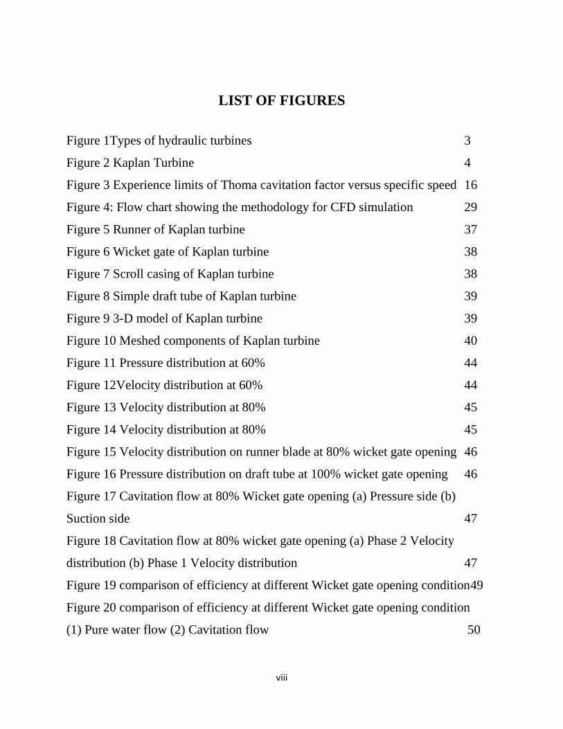
LIST OF FIGURES

Figure 1Types of hydraulic turbines 3

Figure 2 Kaplan Turbine 4

Figure 3 Experience limits of Thoma cavitation factor versus specific speed 16

Figure 4: Flow chart showing the methodology for CFD simulation 29

Figure 5 Runner of Kaplan turbine 37

Figure 6 Wicket gate of Kaplan turbine 38

Figure 7 Scroll casing of Kaplan turbine 38

Figure 8 Simple draft tube of Kaplan turbine 39

Figure 9 3-D model of Kaplan turbine 39

Figure 10 Meshed components of Kaplan turbine 40

Figure 11 Pressure distribution at 60% 44

Figure 12Velocity distribution at 60% 44

Figure 13 Velocity distribution at 80% 45

Figure 14 Velocity distribution at 80% 45

Figure 15 Velocity distribution on runner blade at 80% wicket gate opening 46

Figure 16 Pressure distribution on draft tube at 100% wicket gate opening 46

Figure 17 Cavitation flow at 80% Wicket gate opening (a) Pressure side (b)

Suction side 47

Figure 18 Cavitation flow at 80% wicket gate opening (a) Phase 2 Velocity

distribution (b) Phase 1 Velocity distribution 47

Figure 19 comparison of efficiency at different Wicket gate opening condition49

Figure 20 comparison of efficiency at different Wicket gate opening condition

(1) Pure water flow (2) Cavitation flow 50

ix

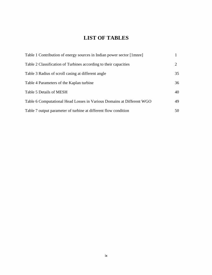
LIST OF TABLES

Table 1 Contribution of energy sources in Indian power sector [1mnre] 1

Table 2 Classification of Turbines according to their capacities 2

Table 3 Radius of scroll casing at different angle 35

Table 4 Parameters of the Kaplan turbine 36

Table 5 Details of MESH 40

Table 6 Computational Head Losses in Various Domains at Different WGO 49

Table 7 output parameter of turbine at different flow condition 50

x

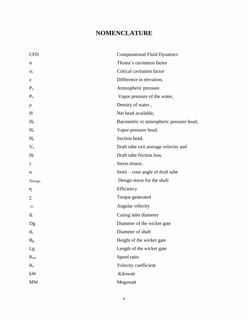
NOMENCLATURE

CFD Computational Fluid Dynamics

σ Thoma’s cavitation factor

σc Critical cavitation factor

z Difference in elevation,

Pa Atmospheric pressure

Pv Vapor pressure of the water,

ρ Density of water ,

H Net head available,

Ha Barometric or atmospheric pressure head,

Hv Vapor pressure head,

Hs Suction head,

Ve Draft tube exit average velocity and

Hf Draft tube friction loss.

τ Stress tensor,

α Semi – cone angle of draft tube

τDesign Design stress for the shaft

ƞ Efficiency

Torque generated ح

ω Angular velocity

di Casing inlet diameter

Dg Diameter of the wicket gate

ds Diameter of shaft

Bg Height of the wicket gate

Lg Length of the wicket gate

Kuo Speed ratio

Kv Velocity coefficient

kW Kilowatt

MW Megawatt

xi

N Rpm of turbine runner

Ns Specific speed of turbine

Pi Pressure at inlet

Po Pressure at outlet

Q0 Quantity of water flowing per second

Rθ Radius of spiral casing at given θ

Ri Radius at casing exit

T Torque on the shaft

Vi Velocity at the inlet to casing

Q Rated discharge

P Power

D Runner diameter

WGO Wicket gate opening

1

CHAPTER 1

INTRODUCTION

1.1 GENERAL

With the rise in population and a positive population growth the demand of power is also

increasing and to generate electricity the resources are limited. The expected time for which

resource will be available is reducing. First is conventional and second is non- conventional. In

conventional energy resources, fossil fuels which produces large amount of greenhouse gases

and pollution. At present in India almost 17%of its total electricity is being produced by

hydropower plants.

Table 1 Contribution of energy sources in Indian power sector [1]

MODES THERMAL NUCLEAR HYDRO RES

INSTALLED

CAPACITY(MW)

180361.89 5780 40867.43 31692.14

1.2 COMPONENTS OF HYDROPOWER PLANT

Components of hydropowerplant can be categorized as following below:

1.2.1 Civil Works Components

Civil works components of hydropower are listed below

Weir

Intake works

Sand trap

Forebay

Power channel

Penstock

1.2.2 Electro-Mechanical Components

2

Electro-Mechanical equipment’s mainly include following

Hydro-Turbine.

Generator

Governor

Gates and valves and other auxiliaries.

1.2.1 Turbine

First turbine was made in 18th century in the form of watermill. From then till now

various types of turbines have been developed for various applications. Main types of turbines

are reaction and impulse turbines.Hydro-Turbine is a machine which converts the water potential

energy into mechanical energy of a rotating shaft which drives an electric generator to produce

electricity.

Power produce by turbine can be written as following:

𝑷 = 𝝆𝒈𝑸𝒉 (1.1)

𝑃 = power

𝑔= gravitational acceleration

ℎ = head

Q = discharge

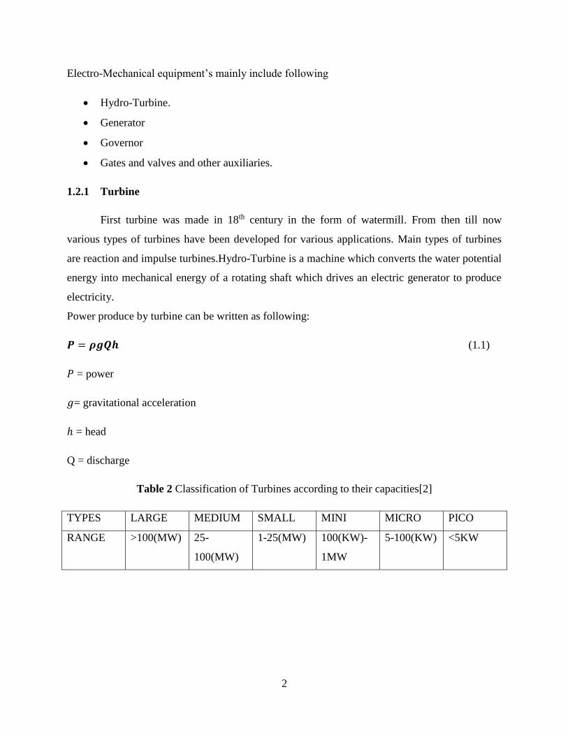
Table 2 Classification of Turbines according to their capacities[2]

TYPES LARGE MEDIUM SMALL MINI MICRO PICO

RANGE >100(MW) 25-

100(MW)

1-25(MW) 100(KW)-

1MW

5-100(KW) <5KW

3

1.3 TYPES OF TURBINE

Impulse Turbine

Reaction Turbine

1.3.1 Impulse Turbine

Impulse turbine uses kinetic energy of the water to produce mechanical energy.in this turbine

water strikes on the bucket and its kinetic energy gets converted into rotational energy of the

runner.

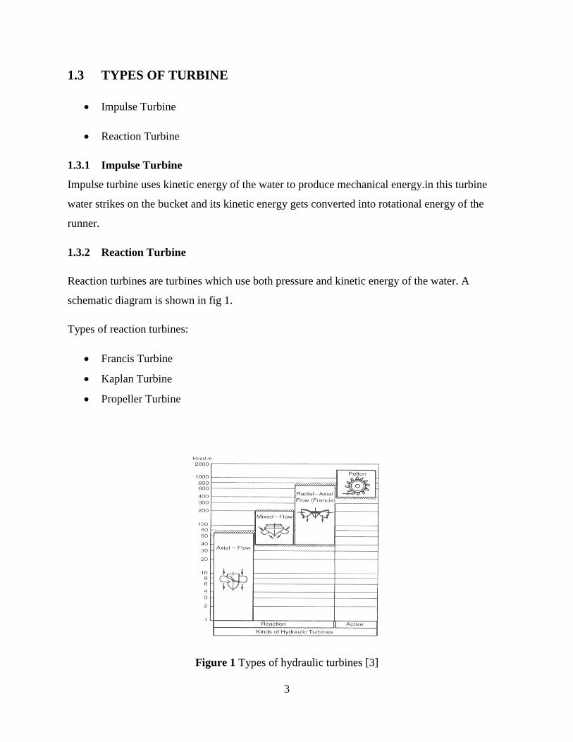
1.3.2 Reaction Turbine

Reaction turbines are turbines which use both pressure and kinetic energy of the water. A

schematic diagram is shown in fig 1.

Types of reaction turbines:

Francis Turbine

Kaplan Turbine

Propeller Turbine

Figure 1 Types of hydraulic turbines [3]

4

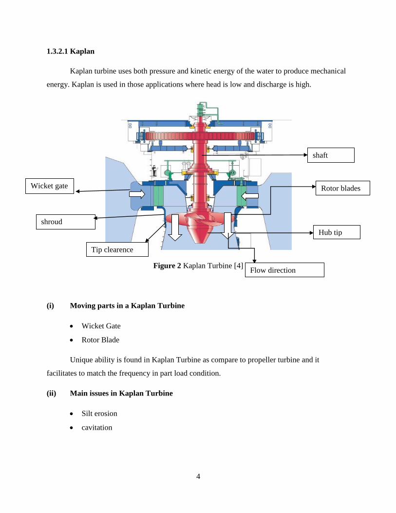
1.3.2.1 Kaplan

Kaplan turbine uses both pressure and kinetic energy of the water to produce mechanical

energy. Kaplan is used in those applications where head is low and discharge is high.

Figure 2 Kaplan Turbine [4]

(i) Moving parts in a Kaplan Turbine

Wicket Gate

Rotor Blade

Unique ability is found in Kaplan Turbine as compare to propeller turbine and it

facilitates to match the frequency in part load condition.

(ii) Main issues in Kaplan Turbine

Silt erosion

cavitation

shroud

Wicket gate

Hub tip

Rotor blades

shaft

Tip clearence

Flow direction

5

(iii) Selected turbine specification

In present study 7MW Kaplan turbine with 15m net head and 125rpm is used.

1.4 STRUCTURE OF THE REPORT

Chapter 2: In this chapter review of literature is done on both experimental and numerical

studies for design of turbine and cavitation.

Chapter 3: In this chapter, brief introduction is given, about cavitation in hydro turbines.

Chapter 4: This chapter describes CFD modelling and various turbulence models used in

present work.

Chapter 5: This chapter contains design of Kaplan turbine of 7MW used in present study.

Chapter 6: It contains results observed from present thesis and analysis.

6

CHAPTER 2

TERMINOLOGY

Turbine

First turbine was made in 18th century in the form of watermill. From then till

now various types of turbines have been developed for various applications.Main types of

turbines are reaction and impulse turbines. Hydro-Turbine is a machine which converts the water

potential energy into mechanical energy of a rotating shaft which drives an electric generator to

produce electricity.

Kaplan Turbine

Kaplan turbine uses both pressure and kinetic energy of the water to produce

mechanical energy. Kaplan is used for low head applications where discharge is high.

Cavitation

Cavitation occurs in turbines only only if local pressure of the turbine goes below the

vapor pressure at operating temperature. If fluid flow is steady then pressure will decrease if

velocity is increasing.

Computational fluid dynamics

Science of predicting fluid flow, heat and mass transfer, and other related phenomenon

by solving mathematical equations which govern these processes using numerical methods is

known as Computational Fluid Dynamics

7

CHAPTER 3

SCOPE OF STUDY

Various numerical studies have been done on Hydro turbines. Turbines show different

flow characteristics on different turbulence models and boundary conditions. Their Flow

behavior also varies with different geometric parameters. So it becomes necessary to investigate

the suitable combination of turbulence models and boundary conditions for turbine according to

their requirements. It is suitable to investigate this using Computational Fluid Dynamics. CFD is

a cost effective approach and gives reliable results in very less time. CFD is the science of

predicting fluid flow, heat transfer, mass transfer, chemical reactions and related phenomenon by

solving mathematical equations which govern these processes using numerical methods.

Present research deals with cavitation in Kaplan turbine with combination of different

boundary conditions and 2-eq turbulence models. Modeling of turbine is done in ANSYS Design

Modeler and MESH is generated in ANSYS 14.0 mesh module. Further analysis is done in

FLUENT solver. Model is validated with previous studies and theoretically both.

8

CHAPTER 4

LITERATURE REVIEW

Turbines are regarded as the most significant component of any hydro power plant. They

cover about 15 – 35 percent of the total project cost. Feasibility of the project depends on the

cost of its components. Many laboratory experiments were carried using physical model to know

the hydrodynamic behavior of the machine. Physical modelling has been one of the methods in

knowing the behavior of the turbine but has been a costly and time consuming technique Since

past two decades computational fluid dynamics has become a powerful tool in analyzing the flow

field of complex turbo machines and has been used extensively during the study for design of the

turbine in order to optimize the design as well as to save time. In this chapter literature review

for design optimization of Kaplan turbine and Cavitation in turbine is described.

Categories of topics

Experimental investigation

Numerical studies

4.2 EXPERIMENTAL INVESTIGATION

Punit Singh and Franz Nestmann [5] detailed experiment investigated on the effects of

exit blade geometry on the part-load performance of low-head axial flow propeller turbines. The

relationship between exit tip angle, discharge, shaft power, and efficiency has presented.

Punit Singh and Franz Nestmann [6] investigated the influence of design parameters in

low head axial flow turbines like height of blade, blade profiles and blade number.by

experimental result developed physical relationship between the two design parameters (blade

height and blade number) and the performance parameters.

4.3 NUMERICAL STUDIES

9

Harsh vats and R.P. Saini [7] investigated the Combined Effect of Cavitation & Silt

Erosion on Francis turbine and concluded that combined effect of sand erosion and cavitation is

more pronounced than their individual effects

Jain et al., 2010 et al [8] studied Two types of methodology are generally used for the

simulation of the turbine depending upon the required objectives. Steady state simulation has

been used to determine the efficiency of the turbine . The nature of flow in turbine is unsteady in

nature due to rotating of the runner. Therefore unsteady state simulations are conducted to know

the transient behavior of the flow and for the investigation of the pressure fluctuation in different

component of the turbine and also the interaction between rotor and stator.

.Taun singh tanwar et al [9] studied. CFD based performance analysis and stress analysis

done on runner blade and guide vane respectively of a Francis turbine. Flow behavior and fatigue

analysis is done respectively and found the life, damage, factor of safety for that particular

model.

Nilsson and Davidson et al [10] studied dissimilar turbulent modelling were found being

used in simulating flow in hydro turbine. In this low Reynolds’s number turbulent models are

being used to resolve the viscous sub layer it also resolve the transition phenomena occurring in

turbine and very useful if there is hub and tip clearance is present in that turbine.

Jain et al[11] studied among the turbulence model in a Francis turbine, k-w shear stress

transport model has been found to give better convergence and turbine performance compared

with standard k-e, Renormalization group (RNG) k-ϵ. SST model has been successful in giving

accurate results for cases where there are adverse pressure gradient flows and where separation

of flow occurs.

Hsing-nan Wu et al [12] investigated the design parameters that affect the performance of

horizontal-axis water turbines by using computational fluid dynamics and Simulation result

validated with experimental result. The result found that the power is directly proportional to

square of radius of runner blade and cubic of velocity.

Dr. Vishnu Prasad [13] CFD analysis done on axial flow turbine at different operating

condition and validated with existing experimental setup result. The variation of computed

10

parameters justifies with the characteristics of axial flow turbine. The computed efficiencies at

some regimes of operation are critically compared with experimentally tested model results and

found to bear close comparison.

Kiran Patel et al [14] investigated CFD analysis of Francis turbine and validated of CFD

result with experimental result. CFD analysis of complete system is conducted at best efficiency

point as well as at part load and performance along with losses of various components predicted.

Predicted CFD analysis results are compared with experimental results and they show good

agreement. This case becomes guidelines for our future new development project.

Alok Mishra and R.P Saini [15] studied, CFD-based performance analysis of Kaplan

turbine for micro hydro range. The operating parameters of the Kaplan turbine have been

optimized using commercial CFD package ANSYS-14. The turbine having rated capacity of 100

kW at rated head and discharge of 1.5 m and 7.03m3/s respectively. Based on CFD analysis it

has been found the total pressure variation is high in the runner and near the wall of the casing.

In the casing maximum value of total pressure has been observed while minimum value of The

efficiency of the Kaplan tubular turbine has been found to be maximum as 91% for design

condition i.e. at rated discharge 7.03m3/s and at rated head 1.5 m at 85% wicket gate opening.

Jacek Swiderski et al [16] investigated practical applications of Computational Fluid

Dynamics (CFD) based on CFX-TASC flow software. Tried to solve reverse problem should

there be a strict mathematical to the N-S equations, the solution to a problem of finding a shape

of flow channel to achieve certain effect would be possible.

Dinesh Kumar et al [17] carried out flow analysis of Kaplan turbine using commercial

CFD package ANSYS 14 at different wicket gate openings. This analysis can be useful to

determine the basic flow physics in various domains. A turbine having rated capacity of 7 MW at

rated head and discharge of 15 m and 47.54 m3/s respectively has been considered for this

analysis. Based on CFD results obtained, it is observed that best efficiency point of turbine is at

80% WGO. The analysis ascertained the trend of losses and flow pattern in various domains. The

numerical simulation results are found in order to be consistent with the real situation. It shows

that ANSYS-14 is able to generate good computational results in an efficient way.

11

PENG YU-cheng et al [18] studied three Gorges hydropower units found Large-area

erosions such as rust and obvious cavitation on the surface of the guide vane. The flow passages

from the inlet of the spiral case to the outlet of the draft tube are included in the computational

domain. The results found that the static pressure on the guide vane surface is much higher than

the critical pressure of cavitation. Cavitation phenomena studied at different depth by using large

eddy simulation technique

Bernd Nennemann and Thi c.vu [19] predicted the Kaplan turbine blade and discharge

ring cavitation, cavitation found at a number of different locations, notably at the blade leading

edge, on the blade suction side, in both tip and hub gaps and on the discharge ring. Cavitation

can result in frosting or pitting in the above-mentioned locations.

BraneSirok et al [20] reviewed new method of the cavitation monitoring was tested on

the model Kaplan turbine, where beside the computer-aided visualization various integral

parameters were simultaneously observed. The procedure tested and performed in different

integral operational regimes. Results of the study indicated that visualization method is the most

appropriate for the cavitation monitoring.

C Deschenes et al [21] studied. CFD based analysis is done on Kaplan turbine numerical

model and prototype and validate their results with experimental data. Flow was reproduced at

best efficiency point after so many results came from flow analysis at different combination of

boundary condition and turbulence models.

Huixuan Shi et al [22] investigated on cavitation in Kaplan turbines are to achieved

Characteristics of sound waves emitted by cavitation, The laws of cavitation intensity varying

with operating states donated by water head and power output, The relationship of cavitation

intensity to cavitation erosion level.

Pardeep Kumar and R.P. Saini [23] reviewed cavitation on hydro turbine. Based on

literature survey various aspects related to cavitation in hydro turbines, different causes for the

dropped performance and efficiency of the hydro turbines and appropriate remedial measures

suggested by various investigators have been discussed.

12

A Rivettiet al [24] studied. CFD based analysis is done on Kaplan turbine numerical

model and prototype measurements were used to validate the transient simulations. In this study

RNG k-𝜀 model is used in ANSYS CFX and in pressure pulsation signals at low frequency, good

argument found both in shape and amplitude.

Santiago et al [25] employed steady and unsteady simulation for the numerical analysis

of the Francis turbine. Boundary conditions were mass flow inlet and opening with pressure

outlet with solid surfaces as walls for both types of simulation. He stated that this type of

boundary condition represents real flow in the turbine. He developed the hill chart of the Francis

turbine to determine its efficiency by 25 simulations with five different openings of guide vanes

4.4 GAPS IDENTIFIED

As reviewed from the literature it was found that

a. For the studies that have been referred in the preceding literature survey, flow analysis

has been done only through steady state simulation of flow with different boundary

conditions, though an unsteady or transient simulation can reveal the flow characteristics

upon varying wicket gate openings. With the limited computational capability, the same

can be achieved by steady state simulation of different wicket gate opening for the same

rotational speed of the runner.

b. Study of cavitation effect on Francis turbine of small hydro power has been

investigated by authors as noted in the literature survey, though such investigations

remain at hand to be carried out for Kaplan turbine in the small hydro range.

c. Study of cavitation on large scale hydropower turbines have revealed that k-ω SST

viscous turbulence model has proven, with great accuracy, helpful in predicting the

generation of vapor and the appropriate vapor fraction values could be estimated in

comparison to the other two equation turbulence models.Investigation of cavitation effect

has been successful for Kaplan turbines but with k-ϵ model, however more accurate

results can be obtained with k-ω SST model, thus such investigation must be carried out.

13

CHAPTER 5

OBJECTIVE OF THE STUDY

The number of hydro plant face sever cavitation problem in turbine which over a period

of time drastically reduce the overall efficiency of power generation system. Investigation of

Kaplan turbine efficiency under effect of cavitation at different boundary condition (i) pressure

inlet and pressure outlet. (ii) mass flow inlet and pressure outlet has not been carried out

extensively and not available in literature. Further, CFD based analysis of hydro turbine

performance is considered as cost effective method and time saving approach.

Keeping this in view, the present study is proposed with the following objectives.

i. To study and work out the design of a Kaplan turbine.

ii. To identify the system and operating parameters.

iii. To carry out the CFD analysis for the performance of Kaplan turbine under different

flow condition.

a. Performance of Kaplan turbine at different wicket gateopening

b. Performance of turbine under cavitation at different boundary conditions.

c. Performance of turbine under cavitation at different turbulence models.

14

CHAPTER 6

CAVITATION

6.1 GENERAL

Cavitation occurs in turbines only when the local pressure of the turbine falls below the

vapor pressure at operating temperature. If fluid flow is steady then pressure will decrease if

velocity is increasing.

6.2 THOMA’S COEFFICIENT

It is usually necessary to specify the operating condition of the hydraulic turbines to

minimize or avoid the cavitation. It is achieved by specifying the geometric parameters of the

turbine to meet the acceptable range bound by a coefficient accepted and named ‘thoma

coefficient’.

𝜎 =𝐻𝑆𝑉

𝐻 (3.1)

𝜎 =

𝑃𝑎−𝑃𝑣𝑔𝜌

−𝑍

𝐻 (3.2)

𝐻𝑠𝑣 = 𝐻𝑎 − 𝐻𝑣 − 𝐻𝑠 +𝑉𝑒

2

2𝑔+ 𝐻𝑓 (3.3)

Where,

𝐻𝑠𝑣 is the net positive suction head (NPSH) which is total absolute head less vapor pressure

head,

𝑍 is the difference in elevation,

𝑃𝑎is the atmospheric pressure,

𝑃𝑣 is the vapor pressure of the water,

15

𝜌 is the density of water ,

H is the net head available,

𝐻𝑎 is barometric or atmospheric pressure head,

𝐻𝑣 is the vapor pressure head,

𝐻𝑠 is the suction head,

Ve is the draft tube exit average velocity and

Hf is the draft tube friction loss.

If the draft tube friction loss and exit velocity head are ignored, then

𝜎 =𝐻𝑎−𝐻𝑣−𝐻𝑠

𝐻 (3.4)

Thoma cavitation factor (σ) for a particular type of turbine is calculated from the Eqn. (3.4) and

is compared with critical cavitation factor (σc) for different types of turbine. Critical cavitation

factor is defined as the minimum value ofσ at which cavitation occurs [26]. If the value of σ is

greater than σc cavitation will not occur in that particular turbine.

The following empirical relationships in terms of specific speed are used for obtaining the value

of σc for different turbines [26]:

For Francis turbine, σc=0.625(Ns /380.78)2 (3.5)

For Propeller turbine, σc=0.28+ {(1/7.5)*(Ns /380.78)}3 (3.6)

For Kaplan turbine, value of σc can be obtained by increasing the σc of Propeller turbine by 10%.

Where,

Ns is the specific speed of turbine.

Limit of Thoma cavitation factor of hydraulic turbines for safe operation can be detected from

the Fig3. The inclined lines in this figure shows for each specific speed, the minimum Thoma

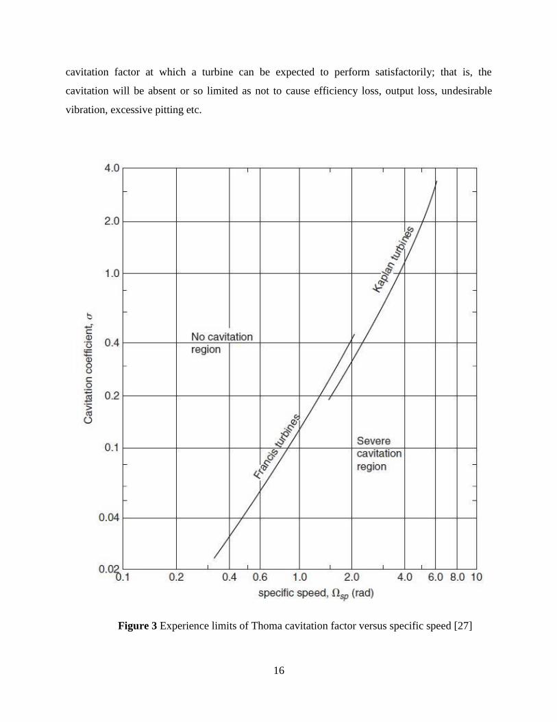
16

cavitation factor at which a turbine can be expected to perform satisfactorily; that is, the

cavitation will be absent or so limited as not to cause efficiency loss, output loss, undesirable

vibration, excessive pitting etc.

Figure 3 Experience limits of Thoma cavitation factor versus specific speed [27]

17

6.3 ELEMENTS INFLUENCING CAVITATION IN HYDROTURBINES

a. Specific speed of the turbine (Ns)

b. Absolute exit velocity

c. Pressure of water (vapor)

d. Total Pressure (absolute)

e. Suction head

f. Fluid’s flow pattern

6.4 EFFECT OF CAVITATION IN HYDROTURBINES

a. Changes in flow pattern

b. Increase in energy damage

c. Huge sound and vibration

d. Corrosion

e. Increase in inefficiency

Different locations in Kaplan turbine at which cavitation occurs

Tip Clearance Cavitation Chamber

Tip Vortex Cavitation

Leading Edge Cavitation

Hub Cavitation

18

6.5 METHODS TO AVOID CAVITATIONS

Cavitation cannot be removed completely but for reduce its occurrence the design of the

turbine should be like this which would avoid the development of low pressure. Parameters like

several point of flow, static pressure should not fall below the vapor pressure.

Material should be cavitation resistant. (Stainless steel, carbon steel).

Temperature of the fluid should be low.

Pressure (static) should be high.

19

CHAPTER 7

CFD MODEL

7.1 INTRODUCTION

Computational fluid dynamics is widely being used to analyze the flow field since last 20

years. It’s capability to solve complex flow phenomena with enhanced software have made it

popular in several fields. X-Y-Z momentum of Navier Stokes equation and continuity equation is

solved numerically. These are differential equations of complex fluid dynamics which requires

discretization of the flow in order to solve them. There are several methods of discretization that

have been used. Finite volume, finite element and finite difference are the three methods that are

currently being used as discretization method for CFD analysis. Among these, finite volume

method is used in CFX in which volume is developed by generating mesh to solve the partial

differential equations of mass, momentum and energy [28].

7.2 HYDRODYNAMICS

The fundamental conservation laws governing the fluid flow in the turbine are:

Conservation of mass: For any period of time mass of a system will remain conserved. The net

mass flow out of the system must be equal to rate of decrease of mass inside the system.

Following equation is the partial differential equation form of the continuity equation.

𝜕𝜌

𝜕𝑡+ ∇. (𝜌𝑉) = 0 (4.1)

Conservation of momentum: Net force applied on the moving fluid is equal to the mass

of an element times its acceleration. Forces acting on the fluid element are body forces which

includes gravitational, electric and magnetic forces and surface forces which are due to the

pressure distribution acting on the surface and the shear stress and normal stress distribution due

to outside fluid. Following is the equation for the conservation of momentum.

𝜌 [𝜕𝑉

𝜕𝑡+ 𝑉. ∇𝑉] = 𝐹𝑏 − ∇𝑝 + 𝜇∇2𝑉 +

𝜇

3∇(∇. 𝑉) (4.2)

These equations are solved for the finite volume element as developed with the meshing

tool and analytical solutions are obtained as required for the study. With proper boundary

20

condition and quality mesh, CFD is able to solve both laminar and turbulent flows. Laminar

flows are easier to solve compared with the turbulent flows as turbulent flows are unsteady in

nature which are developed at high Reynolds’s number. Small scale and large scale eddies are

developed which are three dimensional and random in space and time. There are flow models

developed to solve turbulent flows. Depending upon the requirement of the results, flow models

are selected and computational power required for the simulations depends on these selected

models. Turbulence modelling is solved by Reynolds’s Averaged Navier Stokes (RANS)

equation, large eddy simulation (LES) model and direct numerical modelling (DNS).

Direct numerical simulation gives very accurate result by solving all time and space

scales. However, the grids needs to be very small to resolve spatial and temporal scales and

consumes large computational time. Reynolds’s Averaged Navier Stokes model solves by time

and space averaging. This model provides pretty good result but fails to give accurate results for

transient simulation where variables vary with time.

7.3 TURBULENCE MODELLING

Large scale and small scale eddies are generated due to turbulence in the flow. Various

turbulence models have been developed to capture the effect of these unsteady turbulent eddies.

These models are based on Reynolds’s Averaged Navier Stokes equation which is the sum of

statistically averaged component and fluctuation component.

7.4 SHEAR STRESS TRANSPORT MODEL

Shear stress transport model is the combination of k-e and k- ω model. These two models

are two equation turbulence models whose transport equations are solved along with mass and

momentum equations. The k denotes turbulent kinetic energy, e denotes rate of turbulent

dissipation and ω denotes specific dissipation. The limitations of these two models are

incorporated in SST model. k-e model over predicts the shear stress in adverse pressure gradient

flows and it requires near wall modification as well but still it cannot capture proper flow

separation in the turbulent flow. For proper flow prediction in the near wall layers k- ω model

provides better accuracy then k-e model. However it also fails to predict for separation induced

by high pressure. Shear stress transport model was developed to overcome the limitations of

these two models. With the introduction of blending factors, k- ω and k-e zones are selected

automatically without user interaction at near wall region and away from the surface

21

respectively. This model gives accurate results for the flows with adverse pressure gradient like

in airfoils and flows with separation. Hence, Shear stress transport model is reliable to be used

for turbines [29]

7.5 APPLICATIONS OF CFD

Computational fluid dynamics is a very effective tool and is being used for research in

industries. Applications of CFD are in heat transfer analysis and fluid flow analysis in hydrology

and aerospace.

7.6 NUMERICAL SIMULATION PROCEDURE

To numerical simulation of a physical problem involves approximation of the problem

geometry, choice of appropriate mathematical model and numerical solution techniques,

computer implementation of the numerical algorithm and analysis of the data generated by the

simulation. Thus, this process involves the following steps [30]

I. geometry modeling of the domain associated with the problem.

II. Selection of he best fit mathematical model for physical problem.

III. Selection on appropriate method of discreitization.

IV. grid generation based on the geometry and the discretization method.

V. Selection of technique to solve these equations..

VI. Set appropriate convergence criteria for iterative solution methods.

VII. Prepare the numerical solution for further analysis

7.6.1 Geometry modelling

The numerical simulation needs a computer representation of the problem domain. For

most of the engineering problems, it may not be possible or even desirable to include all the

geometric details of the system in its geometric model. The analyst has to make a careful choice

regarding the level of intricate details to be chosen.

22

7.6.2 Mathematical modelling

Keeping in view the physics of the flow problem and simulation’s objective an

appropriate mathematical model has to be selected. Available computing resources and level of

accuracy desired also have a important role in selecting a mathematical modeling.

7.6.3 Classification of navier-stokes equations

Navier-Stokes equations are coupled nonlinear partial differential equations in four

variables. For mathematical classification, we can look at their linearized form. The formal

classification for incompressible flows is as follows:

I. Steady viscous flows: elliptic.

II. Unsteady viscous flows: parabolic.

Energy equation has the same behavior, i.e. it is elliptic for steady flows, and parabolic, for Time

dependent problems. Unsteady Navier-Stokes and energy equations are in fact parabolic in time

and elliptic in space. Hence, solution of these equations requires (a) one set of initial conditions,

and (b) boundary conditions at all the boundary points for all values to time t > 0. Compressible

Navier-Stokes equations may be considered as mixed hyperbolic, parabolic and elliptic (or

incompletely parabolic) equations. The elliptic equations are more difficult to solve than

parabolic equations, which lend themselves to marching type solution procedure. Thus, in

practice, steady viscous flows are usually converted to unsteady problems, and solved using a

time marching scheme. The solution obtained for large values of time t provides the desired

solution of the steady viscous flow problem.

Navier-stoke’s equation

𝜕𝑦

𝜕𝑥= ∇. (𝜌𝑉𝑉) = 𝜌𝑏 − ∇𝑝 + 2∇[𝜇(𝑠 −

1

3(∇. 𝑉)𝐼] (4.3)

23

7.6.4 Classification of Euler equation

Classification of inviscid flow equations governed by Euler equation is different from

that of Navier-Stokes or energy equations due to complete absence of the second order terms.

The classification of these equations depends on the extent of compressibility. Further, for

compressible flows, flow speed (Mach number, Ma) has a significant role in determining the

behavior of the problem. The formal classification of the inviscid flows is as follow:

I. Inviscid incompressible flows

a. Steady flows: elliptic.

b. Unsteady flows: parabolic.

II. Inviscid compressible flows

a. Steady subsonic flows (Ma < 1): elliptic.

b. Steady supersonic flows (Ma > 1): hyperbolic.

c. Unsteady flows: hyperbolic.

Dependence of the flow behavior on local Mach number makes the solution of steady

inviscid compressible flows pretty complicated. For example, let us consider high speed flow

around a bluff body. Even if the upstream Mach number Ma > 1, in the vicinity of the solid

surface, there exists a subsonic zone as the flow velocity goes to zero at the stagnation point.

Therefore, separate algorithms would be required for numerical simulation of the problem in

subsonic and supersonic zones (whose extent and boundaries are themselves unknown). This

situation has baffled aerodynamicist for a while in early 1960s. A way out was provided by the

time dependent approach to solve a steady problem, since the unsteady Euler equation for

compressible flows is hyperbolic everywhere (irrespective of the local Mach number). In fact

this time dependent approach to steady state is also widely used now for solution of steady state

viscous flows.

24

Euler’s equation

𝜕(𝜌𝑉)

𝜕𝑡+ ∇. (𝜌𝑉𝑉) = 𝜌𝑏 − ∇𝑝 (4.4)

7.6.5 Discretization method

There are many dicretization approaches to convert continuum mathematical model into a

discrete system of algebraic equation. The most popular are the following [31].

I. Finite difference method (FDM)

II. Finite volume method (FVM)

III. Finite element method (FEM)

7.6.6 Grid generation

The problem domain is discretized into a mesh/grid appropriate to the chosen

discretization method. The type of the grid also depends on the geometry of the problem domain.

Structured grid is required for the finite difference method, whereas FEM and FVM can work

with either structured or unstructured grids. In case of unstructured grids, care must be taken to

ensure proper grading and quality of the mesh.

Types of grids

There are three types of grids.

I. Structured grids

II. Block-structure grids.

III. Un-structured grids

Grid generation process

The process of grid generation for complicated geometries normally involves following

steps:

25

I. Decompose the problem domain into a set of sub-domains (blocks)

II. In each block, generate the grid. Typical sequence of operations would be

a. Generate edge-grid (i.e. divide the edges of a surface in desired number of one

dimensional elements).

b. Using the edge grids, generate the grid on the block-surfaces.

c. Use surface grids as input to generate volume mesh.

III. Check mesh quality, and modify the mesh as required.

7.6.7 Numerical solution

The discretization method applied to the mathematical model of the problem leads to a

system of discrete equations: (a) a system of ordinary differential equations in time for unsteady

problems, and (b) a system of algebraic equations for steady state model. For unsteady problems,

time integration methods for initial value problems are employed, some of which transform the

differential system to a system of algebraic equations at each time step. algebraic equations are

solved by iterative method.choice of methods being dependent on the type of the grid and size of

the system..

Solution of discrete algebraic system

Application of FDM, FVM, OR FEM lead to a system of algebraic equation which may

be linear or non-linear depending on the problem

I. Iterative method for linear system:

a. Direct solver (LU decomposition, Gauss elimination etc.)

b. Iterative solver (SOR, Gauss-seidel, PCG etc.)

c. Accelerated iterative method(conjugate gradient, GMRES)

II. Iterative method for nonlinear system:

a. Newton-Raphson method

26

b. Global method (Picard iteration)

c. Mix of global and Newton-Raphson method

III. Time dependent problem:

a. Two level method for first order initial value problem

b. Multi-point method (Adams-Bashforth method)

c. Multi-level predictor-corrector methods

d. Runge-Kuttamethods(these method are two level multi point method)

7.6.6 Post processing

Numerical simulation provides values of field variables at discrete set of computational

nodes. Post processing which involves report generation and understanding flow with different

plots and contours. Numerical simulation provides values of field variables at discrete set of

computational nodes. For analysis of the problem, the analyst would like to know the variation of

different variables in space-time. Further, for design analysis, secondary variables such a stresses

and fluxes must be computed. Most of the commercial CFD codes provide their own

postprocessor which compute the secondary variables and provide variety of plots (contour as

well as line diagrams) based on the nodal data obtained from simulation. These computations

involve use of further approximations for interpolation of nodal data required in integration and

differentiation to obtain secondary variables or spatial distributions

7.6.7 Validation

In present studyKaplan turbine’s 7 MW model is used. It has a rotation speed of 125 and

specific speed of 413 with 15 meter of head and mass flow rate of 47.57 m3/sec. Kaplan Turbine

model is validated with previous studies [17] results and also validated theoretically.

7.6.8 Models available in ANSYS fluent

There are two types of flow problem steady and turbulent. Different models for steady

flow as well as turbulent are present. Laminar flow are characterized by smoothly varying

velocity fields in space and time in which individual laminar move past one another without

generating traverse currents. These flows arise when the fluid viscosity is sufficiently large to

27

damp out any perturbations to the flow that may occur due to boundary imperfections or other

irregularities. These flows occur at low to reasonable values of the Reynolds’s number. The

turbulent model flows are characterized by large nearly random fluctuations in velocity and

pressure in both space and time. These fluctuations occur from instabilities that grow until

nonlinear interactions cause them to break down into finer and finer whirls that eventually are

dissipated (into heat) by the action of viscosity. There are different turbulence models available

in fluent.

i) Spalart-Allmaras model

ii) k-ε models

- Standard k- ε model

- Renormalization-group (RNG) k- ε model

- Realizable k- ε model

iii) k-ω models

- Standard k-ω model

- Shear-stress transport (SST) k- ω model

iv) v2-f model

v) Reynolds stress model (RSM)

vi) Detached eddy simulation (DES) model

vii) Large eddy simulation (LES) model

Mutiphase model available in ANSYS fluent

i) Mixture

ii) Eulerian

iii) Volume of fluid

28

As mentioned above, among these models, k-ω SST model is very popular in industry for

turbulence modelling. This model gives fairly good results. Here in this work k- ω SST model is

used for flow analysis of Kaplan turbine and for cavitation multiphase mixture model is used for

the further analysis.

29

CHAPTER 8

RESEARCH METHODOLOGY

In order to meet the objective of the work, first step will be to size the Kaplan turbine for

the available data of site like discharge and head, which includes obtaining the dimensions of the

turbine and associated components. The dimensions obtain/calculated during sizing of the

turbine to generate the 3-D model of the Kaplan turbine and its assembly components. 3-D

model of the turbine was generated in Design Modeler in ANSYS Workbench 14.0.After

assembling the Kaplan turbine successfully; it has been exported to ‘Mesh’ module of ANSYS.

The generated mesh was transferred to the ‘FLUENT’ module where simulation has been carried

out with the help of suitable turbulence model and the results were obtained.

A flow chart for the methodology to be adopted for the proposed dissertation work is shown in

Fig. 4.

Figure 4: Flow chart showing the methodology for CFD simulation

Select size Parameters

Design and Sizing of Kaplan Turbine

3-D model of Kaplan Turbine in

Design modeler

Assembly of Kaplan Turbine

components

Meshing of 3-d model

Flow simulation of Turbine

Analysis of Kaplan Turbine

30

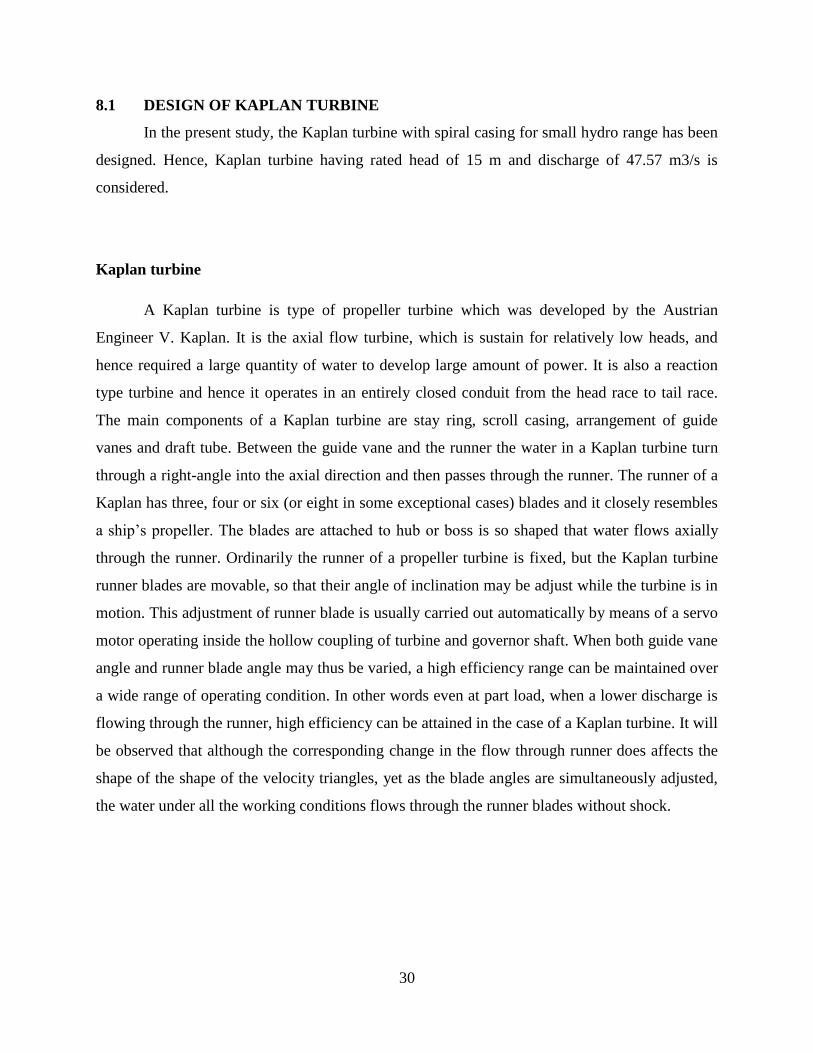
8.1 DESIGN OF KAPLAN TURBINE

In the present study, the Kaplan turbine with spiral casing for small hydro range has been

designed. Hence, Kaplan turbine having rated head of 15 m and discharge of 47.57 m3/s is

considered.

Kaplan turbine

A Kaplan turbine is type of propeller turbine which was developed by the Austrian

Engineer V. Kaplan. It is the axial flow turbine, which is sustain for relatively low heads, and

hence required a large quantity of water to develop large amount of power. It is also a reaction

type turbine and hence it operates in an entirely closed conduit from the head race to tail race.

The main components of a Kaplan turbine are stay ring, scroll casing, arrangement of guide

vanes and draft tube. Between the guide vane and the runner the water in a Kaplan turbine turn

through a right-angle into the axial direction and then passes through the runner. The runner of a

Kaplan has three, four or six (or eight in some exceptional cases) blades and it closely resembles

a ship’s propeller. The blades are attached to hub or boss is so shaped that water flows axially

through the runner. Ordinarily the runner of a propeller turbine is fixed, but the Kaplan turbine

runner blades are movable, so that their angle of inclination may be adjust while the turbine is in

motion. This adjustment of runner blade is usually carried out automatically by means of a servo

motor operating inside the hollow coupling of turbine and governor shaft. When both guide vane

angle and runner blade angle may thus be varied, a high efficiency range can be maintained over

a wide range of operating condition. In other words even at part load, when a lower discharge is

flowing through the runner, high efficiency can be attained in the case of a Kaplan turbine. It will

be observed that although the corresponding change in the flow through runner does affects the

shape of the shape of the velocity triangles, yet as the blade angles are simultaneously adjusted,

the water under all the working conditions flows through the runner blades without shock.

31

Components of Kaplan Turbine

Wicket gate

Wicket gate in Kaplan is same as the guide vanes in Francis turbine. The only difference

is that the guide vane in Francis usually used for guiding the water but in the case of Kaplan

wicket gate used for controlling the work. The wicket gates or guide vane are fixed between two

rings in the form of a wheel known as guide wheel. The wicket gate have a hydrofoil section

which allow water to pass over them without forming eddies and with minimum friction losses.

Each guide vane can be rotated about its pivot center which is connected to the regulating ring by

means of a link and a lever and hence the required quantity of water can be supplied to the

runner by opening or closing the guide vanes. The guide vanes are generally made of cast steel.

Stay Vanes

In case of big units, the stay vanes are provided at the inside circumference of the casing.

The stay vanes provide strength to the casing and also direct the water towards guide vanes.

Runner

The flow in the runner of a Kaplan turbine is purely axial. There is axial entry and exit of

water. The width of the runner depends on the specific speed. The high specific speed runner is

wider than the one which has a low specific speed because the high specific speed runner has to

work with a large amount of water. The runners are made of cast iron for small output, cast steel

for large output and stainless steel or a non-ferrous metal like bronze, when the water is

chemically impure and there is a danger of corrosion.

Shaft and Bearing

The runner is keyed to the shaft which may be vertical or horizontal. The shaft is

generally made of steel. It is provided with a collar bearing for transmitting the axial thrust to the

bearing. The turbine is generally provided with one bearing. In vertical shaft turbine, bearing

carries full runner load and acts as thrust cum supporting bearing. Right selection of bearing is

therefore extremely important.

32

Draft Tube

The water after passing through the runner flows to the tail race through draft tube. A

draft tube is a pipe or passage of gradually increasing cross section area which connects the

runner exit to tail race. It may be made of cast or plate steel or concrete. It must be alright and

under all conditions of operation its lower and must be submerged below the level of water in the

tail race.

Casing

Spiral casing is taken for this study to avoid loss of efficiency, the flow of water from the

penstock to the runner should be such that it will not form eddies. In order to distribute the water

around the guide ring evenly, the scroll casing is designed with cross sectional area reducing

uniformly around the circumference, maximum at the entrance and nearly zero at the tip. This

gives a spiral shape and hence the casing is named as spiral casing.

8.2 SIZING OF KAPLAN TURBINE

Potential of plant [32]

P=9.81*Q*H kW (5.1)

=7000kW

Where Q=rated discharge in (m3/s)

H=net head in (m)

For the present study, the rated potential of the plan has been taken 7000 kW as the convenience

for the design calculation of Kaplan turbine

Specific speed

Ns =N√(P∗1.358)

Hn5/4 (5.2)

N=125 r.p.m

33

Ns= 125√(1000∗1.358)

155/4

Ns=413

N=speed of turbine

Ns=specific speed of turbine

Runner

Outer Diameter of runner has been calculated by the equation which is given below;

D = 84.6×0.0233×NS

2/3⁄×Hn

1/2

𝑁 (5.3)

D = 3.4 m

Hub to tip ratio d/D=0.35

Diameter of hub d=1.2 m

Wicket gate

Diameter (Dg)

Diameter of wicket gates has been calculated by formula which is given below

Dg = 60∗Kug∗√2gH

πN (5.4)

Dg = 3.6 m

Where, Kugis speed ratio, varies from 1.3 to 2.25, increase with the specific speed.

For the present study, the value of the speed ratio (Kug) has been taken 1.38.

34

Height (Bg)

In the case of Kaplan turbine the value of the ratio of Height of the wicket gates and diameter of

runner vary 0.10 to 0.3 according to the specific speed. For the present study, the value of the

ratio has been taken 0.23.

I.e. Bg/D = 0.23

SoBg = 0.8 m

Length (Lg)

Empirical relation between the length and diameter of the wicket gate is given below;

Lg=0.3∗Dg = 1.1 m

No. of wicket gates

Number of wicket gates varies 8 to 24, as increasing diameter of guide wheel.

Let the no. of wicket gate 15 which is suitable for the runner diameter of Kaplan turbine

Scroll casing

Since the diameter of the casing decrease along its path, it takes the shape of a Spiral,

also known as Archimedean Spiral. So, it becomes necessary to know or figure out the

dimensions and coordinate at various angles taken from the centre.

Quantity of water flowing per second, Qo = Vi*π

4*di

2 (5.5)

Where, di is casing inlet diameter and, Vi is the velocity at the inlet to casing (m/s)

Also, Vi= Kv ∙ √2𝑔𝐻 (5.6)

Where, Kv is velocity coefficient.

The maximum value of Vi can be 10 m/s.

Starting with inlet diameter di of the spiral casing, it should be less than or equal to the penstock

diameter. Now Vi is known di, Qo is calculated.

35

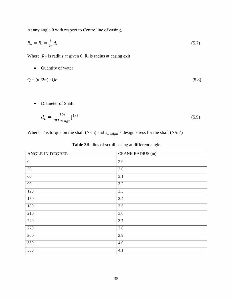
At any angle θ with respect to Centre line of casing,

𝑅𝜃 = 𝑅𝑖 =𝜃

2𝜋𝑑𝑖 (5.7)

Where, 𝑅𝜃 is radius at given θ, Ri is radius at casing exit

Quantity of water

Q = (𝜃 /2𝜋) ∙ Qo (5.8)

Diameter of Shaft

𝑑𝑠 = [16𝑇

𝜋𝜏𝐷𝑒𝑠𝑖𝑔𝑛]1/3 (5.9)

Where, T is torque on the shaft (N-m) and 𝜏𝐷𝑒𝑠𝑖𝑔𝑛is design stress for the shaft (N/m2)

Table 3Radius of scroll casing at different angle

ANGLE IN DEGREE CRANK RADIUS (m)

0 2.9

30 3.0

60 3.1

90 3.2

120 3.3

150 3.4

180 3.5

210 3.6

240 3.7

270 3.8

300 3.9

330 4.0

360 4.1

36

Draft tube

Dimensions of straight divergent type draft tube were carried out using following.

i. Diameter of draft tube at inlet

Di = D2

Where, D2 is diameter of turbine at outlet

Suction head Hs=Ha-Hv-σHnet

Critical thoma coefficient σc = 0.28 + ( 1

7.5(

𝑁𝑠

380.78)3)

σc=0.45

For Kaplan turbine σc=1.1*0.45=0.495

Hs=3.2 m

ii. Semi cone angle

α = 4-8 degree

Semi angle will be taken 5 degree

Table 4 lists the all parameters of the Kaplan turbine which have been computed by using design

in this chapter

Table 4 Parameters of the Kaplan turbine

Rated Head 15m

Rated Dischage 15m3/sec

Rated Turbine output 7MW

Rated Speed 125rpm

No. of Runner Blade 3.4m

Runner diameter 1.2m

Height of Draft tube 3.2m

37

8.3 FLOW ANALYSIS OF KAPLAN TURBINE

Flow analysis of the hydro turbine is a way to predict the flow behavior inside the turbine

under known conditions. It is done to know the inside flow conditions i.e. pressure and velocity

variations to acquire the flow physics. So the flow analysis of the considered turbine is necessary

to validate the designed model with pure water, so that this model can be used for further

research in design, if solution is not converged and other possibility like in interest of improving

performance of turbine, substantial improvement in variables i.e. design optimization is done. A

7 MW Kaplan turbine with spiral casing under rated head of 15 m and 47.57 m3/sec discharge is

considered in this study .The all parameters of the Kaplan turbine have been computed which are

given in table 4. In order to carry out the flow analysis, 3-D modelling is done of each

component of the turbine by using all parameters which are given in table 4. 3-D model of all

components are developed separately. Flow analysis of Kaplan turbine with pure water and with

mixture is discussed below in detail.

8.4 3-D MODELLING OF TURBINE COMPONENTS

3D modelling of turbine components in DESIGN MODELER cad software is the first

step of Flow analysis. DESIGN MODELER is most user friendly software though which

complicated geometry easily can be created.

Runner blade:

By using ANSYS module BLADEGEN blades of turbine has generated, runner is shown in Fig 5

Figure 5 Runner of Kaplan turbine

38

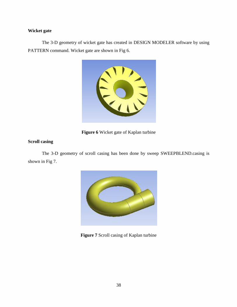
Wicket gate

The 3-D geometry of wicket gate has created in DESIGN MODELER software by using

PATTERN command. Wicket gate are shown in Fig 6.

Figure 6 Wicket gate of Kaplan turbine

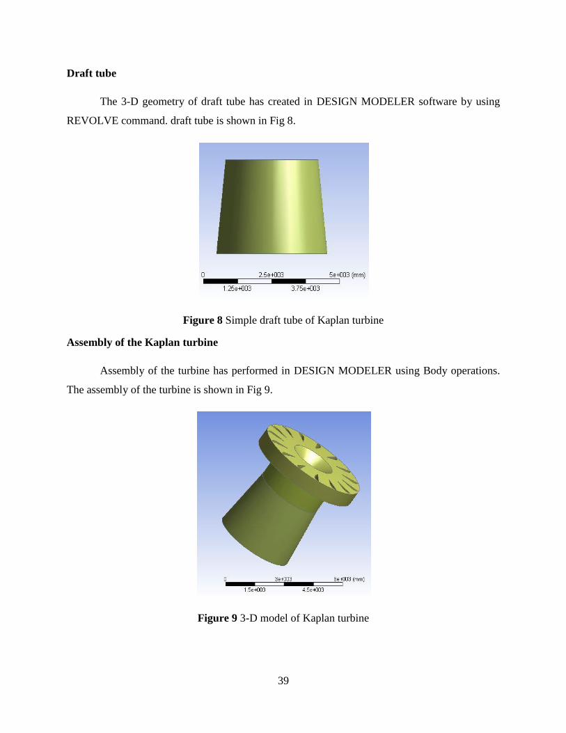
Scroll casing

The 3-D geometry of scroll casing has been done by sweep SWEEPBLEND.casing is

shown in Fig 7.

Figure 7 Scroll casing of Kaplan turbine

39

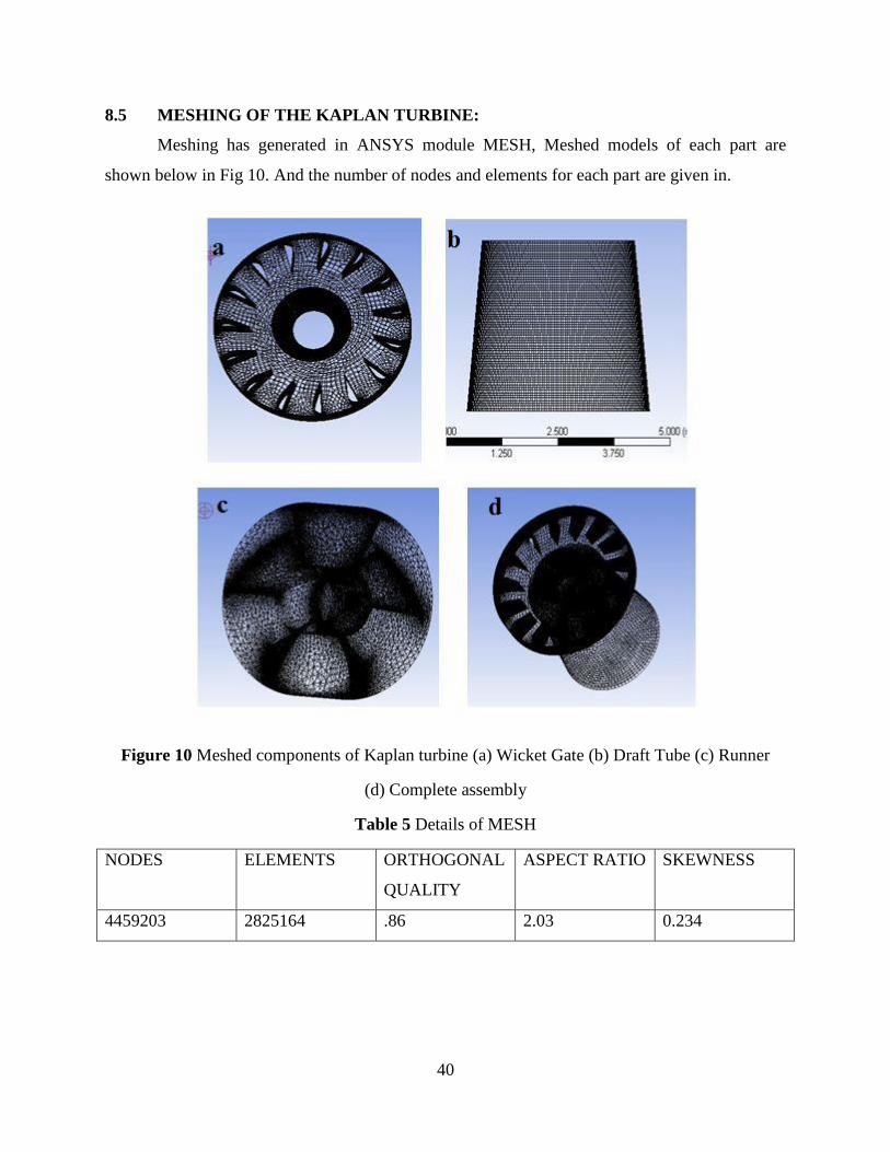
Draft tube

The 3-D geometry of draft tube has created in DESIGN MODELER software by using

REVOLVE command. draft tube is shown in Fig 8.

Figure 8 Simple draft tube of Kaplan turbine

Assembly of the Kaplan turbine

Assembly of the turbine has performed in DESIGN MODELER using Body operations.

The assembly of the turbine is shown in Fig 9.

Figure 9 3-D model of Kaplan turbine

40

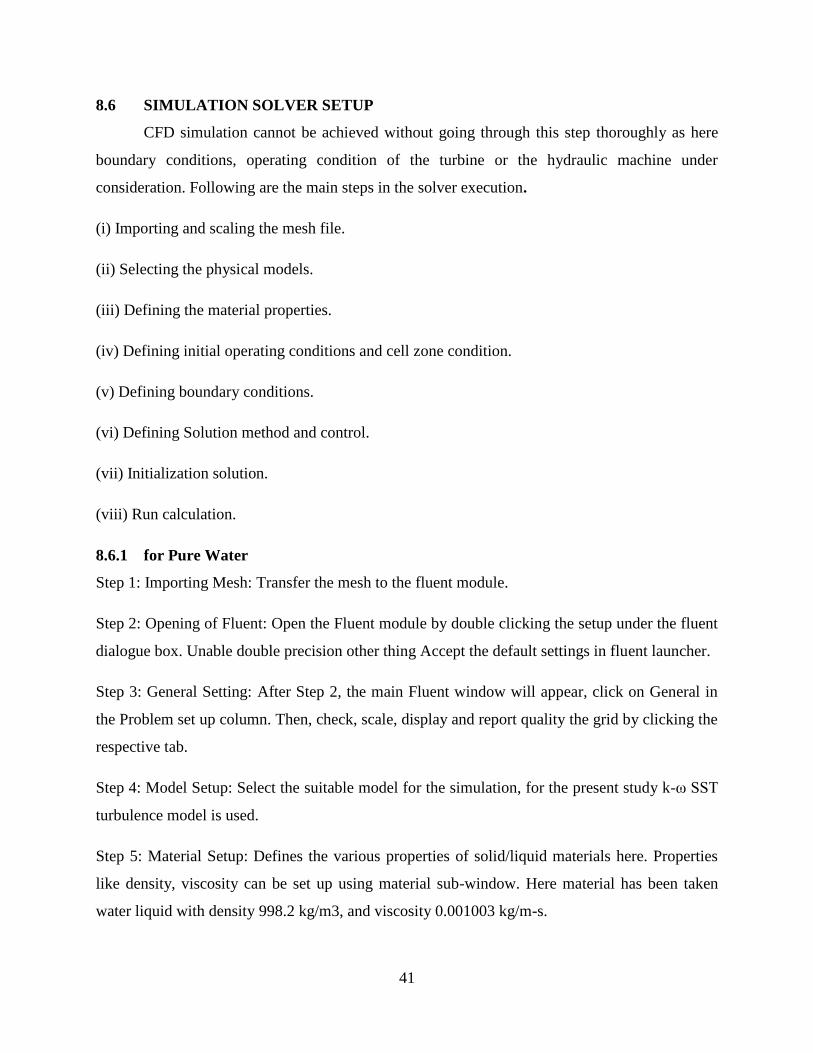
8.5 MESHING OF THE KAPLAN TURBINE:

Meshing has generated in ANSYS module MESH, Meshed models of each part are

shown below in Fig 10. And the number of nodes and elements for each part are given in.

Figure 10 Meshed components of Kaplan turbine (a) Wicket Gate (b) Draft Tube (c) Runner

(d) Complete assembly

Table 5 Details of MESH

NODES ELEMENTS ORTHOGONAL

QUALITY

ASPECT RATIO SKEWNESS

4459203 2825164 .86 2.03 0.234

41

8.6 SIMULATION SOLVER SETUP

CFD simulation cannot be achieved without going through this step thoroughly as here

boundary conditions, operating condition of the turbine or the hydraulic machine under

consideration. Following are the main steps in the solver execution.

(i) Importing and scaling the mesh file.

(ii) Selecting the physical models.

(iii) Defining the material properties.

(iv) Defining initial operating conditions and cell zone condition.

(v) Defining boundary conditions.

(vi) Defining Solution method and control.

(vii) Initialization solution.

(viii) Run calculation.

8.6.1 for Pure Water

Step 1: Importing Mesh: Transfer the mesh to the fluent module.

Step 2: Opening of Fluent: Open the Fluent module by double clicking the setup under the fluent

dialogue box. Unable double precision other thing Accept the default settings in fluent launcher.

Step 3: General Setting: After Step 2, the main Fluent window will appear, click on General in

the Problem set up column. Then, check, scale, display and report quality the grid by clicking the

respective tab.

Step 4: Model Setup: Select the suitable model for the simulation, for the present study k-ω SST

turbulence model is used.

Step 5: Material Setup: Defines the various properties of solid/liquid materials here. Properties

like density, viscosity can be set up using material sub-window. Here material has been taken

water liquid with density 998.2 kg/m3, and viscosity 0.001003 kg/m-s.

42

Step 6: Cell Zone & Operating Conditions Set Up: cell zone condition is defined to set up the

moving frame and stationary frame. In the present study, runner is the only moving frame and

rotating speed is 125 r.p.m, rest is stationary. Operating conditions defines the conditions in

which machinery will be operating like the pressure and direction of Gravitational force. Here

operating condition has been taken as operating pressure 101325 Pascal, gravitational

acceleration 9.81 m/s2 along negative z-direction and Operating temperature 300 K.

Step 7: Boundary conditions: For the present study only two boundary conditions are specified

i.e., at inlet mass flow rate is defined and at outlet i.e., pressure is defined and also provide

moving condition for runner. Mass flow rate is 47570 kg/s and static pressure is 19620 pa.

Intensity has taken 5 % and hydraulic diameter has taken at inlet 3.2 m and outlet 4.2 m.

Step 8: Solution Method: For the present study, SIMPLE method is used with PRESTO and

Second upwind method has been used for solving the turbulence as well as moment.

Step 9: Solution Initialization: standard initialization is used with compute from inlet and

absolute reference has taken.

8.6.2 For Cavitation model

Setting for cavitation model includes following changes in pure water simulation.

Changes are mentioned below:

Step 1: Model: Select k-ω SST turbulence model and mixture multiphase model. Also check the

slip velocity.

Step 2: Phase: Define water-liquid as primary and water-vapor as secondary phase.

Step 3: Define interaction between the phases. Select cavitation mechanism and vapor pressure

taken 3540 Pa and other value take by default.

43

CHAPTER 9

RESULTS & DISCUSSION

9.1 GENERAL

In order to estimate or predict the amount of loss that occurs due to the effect of

cavitation, using CFD performance of Kaplan turbine have been done. In the present analysis,

mass flow rate is taken as 47570 kg/s at full gate opening and wicket gate opening is modeled at

60%, 80%, 100% and 110%. At a 80 % W.G.O analysis is made for single phase pure water

flow.2-phase water with vapor flow is used for cavitation calculation. The static pressure 19620

pa is specified at outlet boundary condition. The reference pressure is taken as 1 atmospheric.

The rotational speed of runner is specified as 125 rpm. The wicket gate and draft tube domains

are taken as stationary. The SST K-ɷ turbulence model has been used and the wall of all

domains is assumed to be smooth with no slip. Coupled arithmetic is applied for coupling

between velocity and pressure.

9.2 ANALYSIS OF RESULT AT DIFFERENT WICKETGATE OPENING

The rotational speed of turbine is taken as the rated speed i.e. 125 rpm, specific speed.The

wicket gate and draft tube domains are taken as stationary. The SST K-ɷ turbulence model has been

used and the wall of all domains is assumed to be smooth with no slip.

9.2.1 Stream line flow pattern for different component

The CFD analysis is carried out by considering steady state single phase at best efficiency

point as well as at part load conditions. The numerical flow analysis is accomplished at four

Wicket gate openings corresponding to four different loading on turbine from best efficiency

point to overload.

(i)For pure Water analysis

The 3-D streamlines and pressure contours at 60% WGO in draft tube are shown in Fig

10 and 11.

44

Figure 11 Pressure distribution at 60%

Figure 12 Velocity distribution at 60%

45

The 3-D streamlines at 80% WGO in Wicket Gate are shown in Fig 13.

Figure 13 Velocity distribution at 80%

The 3-D streamlines and pressure contours at 110% WGO in draft tube are shown in Fig

14.It shows gradual reduction in pressure from casing inlet to exit of runner. It is seen that static

pressure variation in hub region is more at larger wicket gate opening. Velocity profile from

Fig14 inside the turbine assembly indicates that wicket gate and runner domain has smooth

velocity profile whereas as soon as water enters draft domain velocity starts decreasing and

profile becomes non-uniform.

Figure 14 Velocity distribution at 80%

46

The velocity is more and pressure is less on suction side and velocity is less and pressure

is more on pressure side of runner blades..indicate that low velocity zone is formed at diverging

side of passage. The velocity decreases and pressure increases from the runner domain to exit of

draft tube.

Velocity and Pressure distribution on rotor blade shown in Fig 15

(a) (b) (c)

Figure 15 Velocity and Pressure distribution on runner blade at 80% wicket gate opening

(a)Velocity distribution (b) Pressure contour at Pressure side (c) Pressure contour at suction side

pressure contour pattern within draft tube shown in Fig 15

Figure 16 Pressure distribution on drafttube at 100% wicket gate opening

47

For Cavitation flow analysis

Vapor volume fraction distribution on the runner blade shown in Fig 16

Figure 17 Cavitation flow at 80% Wicket gate opening (a) Pressure side (b) Suction side

Velocity distribution on the runner blade shown in Fig 17

Figure 18Cavitation flow at 80% wicket gate opening (a) Phase 1 Velocity distribution at rotor

blade(b) Phase2 Velocity distribution at rotor blade

From the results it has been seen that velocity is increasing towards the tip and because of

that vapor bubble generates at that point.

1.Tip Cavitation

2. Leading edge cavitation

48

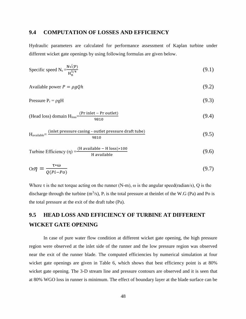
9.4 COMPUTATION OF LOSSES AND EFFICIENCY

Hydraulic parameters are calculated for performance assessment of Kaplan turbine under

different wicket gate openings by using following formulas are given below.

Specific speed Ns =N√(P)

Hn5/4 (9.1)

Available power 𝑃 = 𝜌𝑔𝑄ℎ (9.2)

Pressure Pr = ρgH (9.3)

(Head loss) domain Hloss=(Pr inlet − Pr outlet)

9810 (9.4)

Havailable= (inlet pressure casing – outlet pressure draft tube)

9810 (9.5)

Turbine Efficiency (η) = (H available − H loss)∗100

H available (9.6)

Or𝜂 =τ∗ω

𝑄(𝑃𝑖−𝑃𝑜) (9.7)

Where τ is the net torque acting on the runner (N-m), ω is the angular speed(radian/s), Q is the

discharge through the turbine (m3/s), Pi is the total pressure at theinlet of the W.G (Pa) and Po is

the total pressure at the exit of the draft tube (Pa).

9.5 HEAD LOSS AND EFFICIENCY OF TURBINE AT DIFFERENT

WICKET GATE OPENING

In case of pure water flow condition at different wicket gate opening, the high pressure

region were observed at the inlet side of the runner and the low pressure region was observed

near the exit of the runner blade. The computed efficiencies by numerical simulation at four

wicket gate openings are given in Table 6, which shows that best efficiency point is at 80%

wicket gate opening. The 3-D stream line and pressure contours are observed and it is seen that

at 80% WGO loss in runner is minimum. The effect of boundary layer at the blade surface can be

49

seen at 80% WGO. Similarly the pressure and velocity contour variation on suction and pressure

side of the runner is smoother at 80% WGO as compared to other operating regimes.

Table 6 Computational Head Losses in Various Domains at Different WGO

WGO

Wicket gate

loss (m)

Runner

Loss(m)

Draft tube

Loss(m)

Total losses

(m)

Turbine

Efficiency

(%)

60% .86 1.1 .42 2.38 84.09

80% .83 .93 .32 1.89 87.39

100% .6 .98 .53 2.11 85.92

110% .55 1.3 .61 2.46 83.55

Figure 18 comparison of efficiency at different Wicket gate opening condition

50

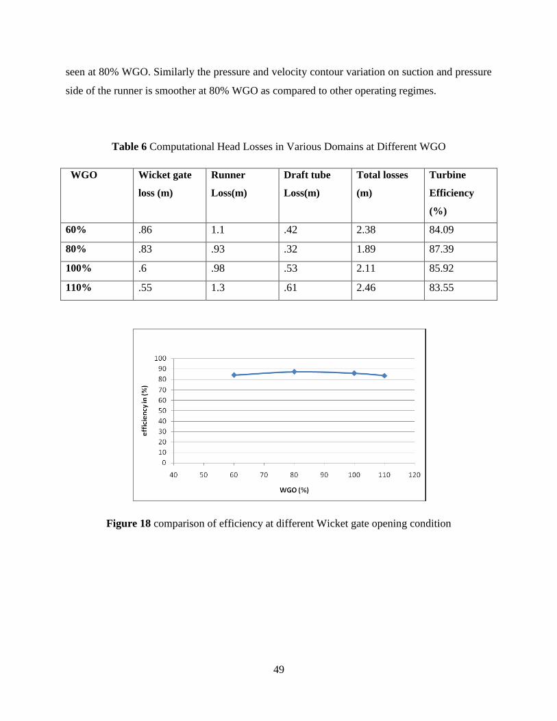
9.6 COMPARISON OF EFFICIENCY AT DIFFERENT FLOW

CONDITION

The efficiency of Kaplan turbine has been calculated at different flow condition. Maximum

efficiency is 85.90 % has been found at 100 % W.G.O for pure water flow, in two phase

cavitation flow efficiency has been reduced by 0.96 %.

Table 7Output parameter of turbine at different flow condition

Flow condition Pressure (pa)

inlet

Pressure (pa)

outlet

Torque(N-m)

Mass flow rate

(m3/s)

Pure 164053 19602 451125 47.67

Cavity 164053 19602 446070 47.57

Figure 19 comparison of efficiency at different Wicket gate opening condition

(1) Pure water flow (2) Cavitation flow

51

CHAPTER 10

CONCLUSIONS AND FUTURE SCOPE

Under the present study of CFD based analysis of small hydro Kaplan turbine of 7 MW

capacity, the effect of cavitation has been studied and analyzed. The turbine analyzed hereby

works under the reaction principle to generate mechanical energy from the hydro energy with

available head of 15 m. The flow analysis was carried out using Computational Fluid Dynamics

using the FLUENT v 14 module available in University computational facility.

The following analysis were carried out during this study:

i. Study of single phase water based flow analysis to predict and validate the performance

of the computational model.

ii. Study of two phase flow, including liquid water and water vapor, where water vapors are

generated due to pressure reducing below the vapor pressure of water at 25o C to simulate

the effect of cavitation.

iii. Study of effect of cavitation on the performance of the Kaplan turbine, provided other

conditions remain same.

The following conclusions drawn from CFD simulation of the Kaplan turbine for four flow

conditions:

i. Based on CFD results obtained for single phase flow of water under the boundary

conditions mentioned in the preceding chapters, it is observed that best efficiency point

(BEP) of turbine is at 80% WGO and head losses are also found minimum at this gate

opening.

ii. For the single phase water flow at different part load conditions, the different values of

efficiency have been obtained as 84.09 %, 87.39%, 85.92% and 83.55% at different

WGO, i.e.60%, 80%, 100% and 110% respectively.

iii. Under the two phase flow, vapor with water, the cavitation is found at suction side of the

blade, blade rim and at outlet of the blade. The efficiency of turbine has been reduced by

0.96 % due to cavitation erosion.

In Computational Fluid Dynamics, the results of the flow analysis are highly dependent on

the geometry of elements composing the flow domain. Although the mesh has been developed to

accommodate greater detail to flow behavior at critical passages of water over blades and inlet

52

passage, there still lies vast opportunity in organizing the mesh structure to further improve the

accuracy of the results to match with the field study or a prototype analysis.

The mesh, as is employed is tetrahedron based control volumes, provide good results for

complicated geometry of rotating fluid machinery. Though, the upcoming hexahedral mesh may

be employed in a possible future work to observe the comparison of effectiveness.

The flow analysis involving cavitation has revealed the locations in the flow domain,

where the bubbles of vapor are generated and displayed in the results in the form of vapor

fraction concentration. These results are valid against the experimental investigation by

Deschenes C et al [21]. A more elaborated experimental study can be done in a follow up work

by studying the effect of this cavitation on the metallic surfaces by using a towing tank for the

flow and rheological analysis of one hydrofoil based turbine blade.

53

REFERENCES

[1] http://www.mnre.gov.in/Ministry of New and Renewable Energy,Govt. Of India. Accessed

on 31/1/2015

[2] http://www.mnre.gov.in/Ministry of New and Renewable Energy,Govt. Of India. Accessed

on 31/1/2015

[3]http://www.mcnallyinstitute.com. Accesed on 31/1/2015

[4] http://www.voith.com. Accesed on 31/1/2015

[5] Punit Singh, Franz Nestmann, “Exit blade geometry and part-load performance of small

axial flow propeller turbines: An experimental investigation”, Experimental Thermal and

FluidScience 34 (2010) 798–811.

[6]Punit Singh, Franz Nestmann, “Experimental investigation of the influence of blade height

and blade number on the performance of low head axial flow turbines”, Renewable Energy

36(2011) 272-281.

[7] Harsh Vats & R.P. Saini. “Investigation on combined effect of cavitation and silt erosion on

Francis turbine”. International Journal of Mechanical and Production Engineering (IJMPE)

ISSN 2315-4489, Vol-1, Iss-1, 2012.

[8] Jain, S., R. P. Saini, and A. Kumar. 2010.”Cfd Approach for Prediction of Efficiency of

Francis Turbine”.

[9] Tarun Singh Tanwar, DharmendraHariyani and Manish Dadhich, “Flow simulation & static

structural analysis of a radial turbine”, IJMET Volume 3, Issue 3, September - December

(2012), pp. 252-269.

[10]Nilsson, H., and L. Davidson. 2003.“Validations of CFD Against Detailed Velocity

andPressure Measurements in Water Turbine Runner Flow”. International Journal for

NumericalMethods in Fluids: 863–879.

[11] Jain and Kokubu 2011. “CFD study of different turbulence models in kaplan turbine”.

54

[12] Hsing-nan Wu, Long-jengChen , Ming-hueiYu , Wen-yiLi , Bang-fuhChen. “On Design

and performance prediction of the horizontal-axis water turbine”, Ocean Engineering 50 (2012)

23–30.

[13] Dr. Vishnu Prasad, “Numerical simulation for flow characteristics of axial flow hydraulic

turbine runner”, Energy Procedia 14 (2012) 2060 – 2065.

[14]Kiran Patel, Jaymin Desai, Vishal Chauhan and ShahilCharnia. “Development of Francis

Turbine usingComputational Fluid Dynamics”. The 11th Asian International Conference

onFluid Machinery and The 3rd Fluid Power Technology Exhibition, Paper ID

AICFM_TM_016November 21-23, 2011, IIT Madras, Chennai, India.

[15] Alokmishra, R.P. Saini and M.K. Singhal. “CFD Based Performance Analysis of

KaplanTurbine for Micro Hydro Power”. International Conference on Mechanical and

IndustrialEngineering, 2012 .

[16] JacekSwiderski. “Recent approach to refurbishments of small hydro projects based on

numerical flow analysis”. Small Hydro Workshop. Montreal 2004.

[17] Dinesh kumar,Saurabhsangal and R.P. Saini. “flow analysis of Kaplan hydraulic turbine by

computational fluid dynamcs”. IJAER, ISSN 0973-4562,Vol-8, Iss-6,pp-61-64, 2013.

[18] Peng Yu-cheng, Chen Xi-yang, CAO Yan, HOU Guo-xiang. “Numerical study of cavitation

on the surface of the guide vane in three gorges hydropower unit”.journal of

hydrodynamic2010,22(5):703 -708 DOI: 10.1016/S1001-6058(09)60106-2.

[19] Bernd Nennemann, Thi C. vu. “Kaplan turbine blade and discharge ring cavitation

prediction using unsteady CFD”.2nd IAHR International Meeting of the Workgroup

onCavitation and Dynamic Problems in Hydraulic Machinery and Systems

Timisoara,RomaniaOctober 24 - 26, 2007.

[20] BraneSirok, MakoHoEevar, Igor Kern, Matej Novak. “Monitoring of the Cavitation in the

Kaplan Turbine”, ISIE‘99 - Bled, Slovenia.

[21] C Deschenes, G D Ciocan, V De Henau, F Flemming, J Huang, M Koller, F A Naime, M

Page,RQian and T Vu“General overview of axial turbine project- a partnership for low head

55

turbine development”. Members of the Scientific Committee of the Consortium on Hydraulic

Machines from:

[22] Huixuan Shi, Xuezheng Chu, Zhaohui Li, Qingfu Sun. “Experimental Investigations on

Cavitation in Large Kaplan Turbines”, 2011 Third International Conference on

MeasuringTechnology and Mechatronics Automation.

[23] Pardeep Kumar, R.P. Saini. “Study of cavitation in hydro turbines—A

review”,Renewableand Sustainable Energy Reviews 14 (2010) 374–383.

[24] A Rivetti, CLucino, S Liscia, D Muguerza and F Avallan. “Pressure pulsation in Kaplan

Turbine”.

[25] Laín, S., M. García, B. Quintero, and S. Orrego. 2010.“CFD Numerical Simulations of

Francis Turbines”. RevistaFacultad De Ingeniería Universidad De Antioquia (51): 24–33.

[26] Dr. R.K. BANSAL “Fluid Mechanics and Hydraulic Machine”.

[27]Pande V K, “Effect of hydraulic design of Pelton turbines on damage due to silt erosion and

its reduction”. PowerPoint presentation, BHEL.

[28]Chung, T. J. “Computational Fluid Dynamics. 2nd Ed., Cambridge University Press,

Cambridge, UK”.

[29] Date, A. W. “Introduction to Computational Fluid Dynamics. Cambridge University Press,

Cambridge”.

[30] http://www.cfd-online.com/Accessed on 31/1/15.

[31] Versteeg, H. K. and Malalasekera, W. M. G. (2007). “Introduction to Computational Fluid

Dynamics”: The Finite Volume Method. Second Edition (Indian Reprint) Pearson Education.

[32] NHPC guidelines for selection of turbines, preliminary dimensioning and layout of surface

hydroelectric power houses.(1993-07)

56

LIST OF PUBLICATION

Munendra Kumar and Alok Nikhade. “Cavitation in Kaplan Turbines – A Review” Journal of

Material Science and Mechanical Engineering, ISSN: 2393-9095 Vol. 2, Number 5, April-

june2015, pp 425-429.