Proceedings of the 7 th International Symposium on Cavitation CAV2009 – Paper No. 91

August 17-22, 2009, Ann Arbor, Michigan, USA

1

Cavitation in a bulb turbine

Jörg Necker Voith Hydro Holding GmbH&Co.Kg.

Heidenheim, Germany

Thomas Aschenbrenner Voith Hydro Holding GmbH&Co.Kg.

Heidenheim, Germany

Winfried Moser Voith Hydro Holding GmbH&Co.Kg.

Heidenheim, Germany

ABSTRACT

The flow in a horizontal shaft bulb turbine is calculated as a two-phase flow with a commercial Computational Fluid Dynamics (CFD-)-code including cavitation model. The results are compared with experimental results achieved at a closed loop test rig for model turbines.

On the model test rig, for a certain operating point (i.e. volume flow, net head, blade angle, guide vane opening) the pressure behind the turbine is lowered (i.e. the Thoma-coefficient σ is lowered) and the efficiency of the turbine is recorded. The measured values can be depicted in a so-called σ−break curve or η-σ−diagram. Usually, the efficiency is independent of the Thoma-coefficient up to a certain value. When lowering the Thoma-coefficient below this value the efficiency will drop rapidly. Visual observations of the different cavitation conditions complete the experiment.

In analogy, several calculations are done for different Thoma-coefficients σ and the corresponding hydraulic losses of the runner are evaluated quantitatively. Besides, the fraction of water vapour as an indication of the size of the cavitation cavity is analyzed qualitatively.

The experimentally and the numerically obtained results are compared and show a good agreement. Especially the drop in efficiency can be calculated with satisfying accuracy. This drop in efficiency is of high practical importance since it is one criterion to determine the admissible cavitation in a bulb-turbine. The visual impression of the cavitation in the CFD-analysis is well in accordance with the observed cavitation bubbles recorded on sketches and/or photographs.

INTRODUCTION

A bulb-turbine is a double regulated turbine in which the Kaplan runner and the generator are mounted on a horizontal shaft. The shaft bearings and the generator are located in a bulb-housing which is supported by piers and which is completely surrounded by water. A common design of a bulb-

turbine is completed by an intake, the guide vanes and the drafttube and is shown in figure 1.

figure 1: sketch of a bulb turbine

A bulb-turbine is most adequate to be used for large flow rates and low head conditions. These conditions can be found for example in run-of-rivers power plants.

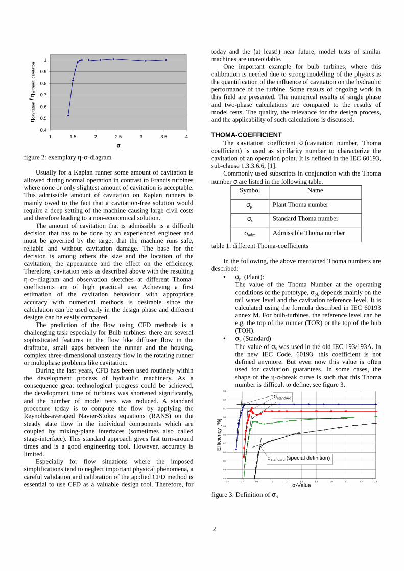
In general, cavitation has different aspects for a water turbine: depending on the intensity and location, the blades can get damaged, vibration can be induced, the performance can deteriorate, and the discharge through the turbine can change significantly. Especially the drop in performance as a function of the Thoma-number σ is of high importance and can be seen exemplary in figure 2. Since the phenomenon cavitation - to be explicitly distinguished from cavitation damage - may occur in horizontal bulb-turbines even in normal operation, there is a strong necessity to predict the cavitation - and, as a consequence, implicitly the drop in performance - as accurate as possible.

2

0.4

0.5

0.6

0.7

0.8

0.9

1

1 1.5 2 2.5 3 3.5 4

σσσσ

ηη ηη cav

itatio

n /

ηη ηη with

out_

cavi

tato

n

figure 2: exemplary η-σ-diagram

Usually for a Kaplan runner some amount of cavitation is

allowed during normal operation in contrast to Francis turbines where none or only slightest amount of cavitation is acceptable. This admissible amount of cavitation on Kaplan runners is mainly owed to the fact that a cavitation-free solution would require a deep setting of the machine causing large civil costs and therefore leading to a non-economical solution.

The amount of cavitation that is admissible is a difficult decision that has to be done by an experienced engineer and must be governed by the target that the machine runs safe, reliable and without cavitation damage. The base for the decision is among others the size and the location of the cavitation, the appearance and the effect on the efficiency. Therefore, cavitation tests as described above with the resulting η-σ−diagram and observation sketches at different Thoma-coefficients are of high practical use. Achieving a first estimation of the cavitation behaviour with appropriate accuracy with numerical methods is desirable since the calculation can be used early in the design phase and different designs can be easily compared.

The prediction of the flow using CFD methods is a challenging task especially for Bulb turbines: there are several sophisticated features in the flow like diffuser flow in the drafttube, small gaps between the runner and the housing, complex three-dimensional unsteady flow in the rotating runner or multiphase problems like cavitation.

During the last years, CFD has been used routinely within the development process of hydraulic machinery. As a consequence great technological progress could be achieved, the development time of turbines was shortened significantly, and the number of model tests was reduced. A standard procedure today is to compute the flow by applying the Reynolds-averaged Navier-Stokes equations (RANS) on the steady state flow in the individual components which are coupled by mixing-plane interfaces (sometimes also called stage-interface). This standard approach gives fast turn-around times and is a good engineering tool. However, accuracy is limited.

Especially for flow situations where the imposed simplifications tend to neglect important physical phenomena, a careful validation and calibration of the applied CFD method is essential to use CFD as a valuable design tool. Therefore, for

today and the (at least!) near future, model tests of similar machines are unavoidable.

One important example for bulb turbines, where this calibration is needed due to strong modelling of the physics is the quantification of the influence of cavitation on the hydraulic performance of the turbine. Some results of ongoing work in this field are presented. The numerical results of single phase and two-phase calculations are compared to the results of model tests. The quality, the relevance for the design process, and the applicability of such calculations is discussed.

THOMA-COEFFICIENT

The cavitation coefficient σ (cavitation number, Thoma coefficient) is used as similarity number to characterize the cavitation of an operation point. It is defined in the IEC 60193, sub-clause 1.3.3.6.6, [1].

Commonly used subscripts in conjunction with the Thoma number σ are listed in the following table:

Symbol Name

σpl Plant Thoma number

σs Standard Thoma number

σadm Admissible Thoma number

table 1: different Thoma-coefficients

In the following, the above mentioned Thoma numbers are described:

• σpl (Plant): The value of the Thoma Number at the operating conditions of the prototype, σpl, depends mainly on the tail water level and the cavitation reference level. It is calculated using the formula described in IEC 60193 annex M. For bulb-turbines, the reference level can be e.g. the top of the runner (TOR) or the top of the hub (TOH).

• σS (Standard) The value of σs was used in the old IEC 193/193A. In the new IEC Code, 60193, this coefficient is not defined anymore. But even now this value is often used for cavitation guarantees. In some cases, the shape of the η-σ-break curve is such that this Thoma number is difficult to define, see figure 3.

83

84

85

86

87

88

89

90

91

92

93

0.5 0.7 0.9 1.1 1.3 1.5 1.7 1.9 2.1 2.3 2.5

σ-Value

Effi

cien

cy [%

]

σstandard (special definition)

σstandard

figure 3: Definition of σS

3

• σadm (admissible)

As described above, some amount of cavitation is allowed in Bulb-turbines due to economical reasons. The admissible amount of cavitation must be defined by the supplier to guarantee a safe and reliable operation of the machine. Below this σadm the continous operation will lead to severe damage of the machine (e.g. heavy erosion of the blade) or even destruction.

EXPERIMENTAL SET UP The model tests were conducted on the low pressure test

rig in the Voith Hydro laboratory in Germany, [2]. The test rig is especially designed for low head machines like bulb- or vertical Kaplan-turbines. The main components are the circuit pump, the head and tail water tanks, and the model turbine driving a motor-generator. They are depicted in figure 4 except of the circuit pump through which the tail and the head water tank are connected.

figure 4: sketch of test rig

For the quantitative analysis of the machine, basic physical quantities are measured: pressure, forces, speed, temperature, [3]. The static pressures at the high pressure side is measured in the intake, upstream of the runner while the pressure at the low pressure side pS is measured at the end of the drafttube. The net head is obtained using the pressure difference and the averaged velocities at the two measuring planes. Measuring the torque via force and well known lever arm, the speed of the runner, the volume flow with an electro-magnetic flow meter and using the evaluated net head, the efficiency of the runner can be evaluated.

The pressure level of the test rig can be changed by changing the absolute pressure in the tail water tank. By evacuating or filling air into the dome of the tail water tank, different suction heads i.e. different Thoma coefficients can be adjusted. The speed of the turbine is usually kept constant.

The sigma value can be calculated with the measured pressures according to

( )

H

hgpp

Svaamb −⋅

−= ρσ

The density and the vapour pressure are concluded from the measured temperature of the water. The ambient pressure is measured. The suction head hS is obtained from the measured low pressure pS and the correction head between the reference

level of the pressure manometer and the pressure tabs in the model. NUMERICAL MODEL

The CFD-code used for the calculations is the commercial software CFX 11.0 of Ansys, [4]. In CFX, the three-dimensional Reynolds-Averaged Navier-Stokes (RANS) equations are solved in conservative form on structured multi-block grids. A finite volume based discretisation scheme is used which is up to second order accurate for the convective fluxes and truly second order accurate for the diffusive fluxes. Time dependent computations can be performed with a second order accurate time stepping scheme. A turbulence model is needed to close the equation system which results from the Reynolds-averaging. A variety of different turbulence models can be applied depending on the application. Here, the SST - model was used which takes advantage of the strength of the k-ε− (free-flow) and the k-ω−model (close to wall). The turbulence model is still one of the largest error sources in modern CFD. However, methods with less or even no modeling are even nowadays not applicable on technical problems, so that the shortly described RANS is the state-of-the-art for the simulation of complex, three dimensional flows.

The calculations are done in stationary mode. The calculation domain consists of the two components guide-vane and runner. It begins upstream of the guide-vanes and ends below the runner, see figure 5. Periodicity in the runner and the guide-vane domains are used. The two components are coupled with a general grid interface with circumferential averaging (stage interface). In the runner domain, the gaps between runner tip and the housing and between the runner and the hub are included in the model. The number of cells used in the guide-vane domain is 260000 nodes and in the runner domain 610000 nodes.

figure 5: considered domain for the CFD

The cavitation is modelled with a homogenous multi-phase model that is based on the Rayleigh-Plesset equation for bubble-growth. The equations for the mass-transfer are

4

( )

−⋅⋅⋅−

−⋅−⋅

=

>

∞

<

∞

∞

∞

va

va

ppl

vavvcond

ppl

vavvnucvap

vpp

R

rF

pp

R

rrF

S

ρρ

ρρ

323

3213

with rv as the volume fraction vapour, rnuc as the volume fraction of the nuclei, R as the initial radius of the nuclei, and Fvap and Fcond as empirical constants. The derivation and the parameters in this model are extensively discussed in Stoltz [5]. For the presented calculations, the standard parameters are taken as proposed by Ansys.

Initialized by a single-phase calculation, the two-phase calculations are started with different static pressures pS at the outlet of the domain. For a given static pressure at the outlet, the corresponding σ can be calculated according to

( )H

gppp Svaamb

⋅+−

= ρσ

*

For a better comparison with the experiment, the static pressure at the outlet of the runner domain has to be transferred to the static pressure at the measuring plane of the experimental configuration. This was done with an additional CFD-calculation extending the so far described domain by the drafttube. The static pressure increase between the outlet of the runner and the measuring plane in the drafttube resulted to be approximately 35.4 kPa. A simple check with Bernoulli verified the order of magnitude of the result (34.8 kPa).

An operating point close to the rated point (in this case maximum power and maximum discharge at the rated head) was chosen for the calculation. As physical boundary condition the same massflow as in the experiment was described for all operation conditions. The σpl,TOH for this head and this machine setting is 2.25 and the σpl,TOR is 2.11. The different pressures at the outlet resulted in the following 11 sigma-values:

2.272 2.113 1.954 1.875 1.835 1.795 1.716 1.636 1.478 1.319 1.160

table 2: in CFD-calculation considered σ-values RESULTS

For each CFD-calculation the relative hydraulic loss of the runner is evaluated. The absolute loss is calculated as the total pressure difference on a plane upstream and downstream of the runner and referred to the rated head (figure 6).

( )rated

tottotabs Hg

pp

⋅⋅−

=ρ

ζ 2,1,

with 2/1,totp as the mass flow averaged total pressure at plane

1 and 2.

figure 6: evaluation planes (green) in the runner domain

The relative loss for the CFD-calculation is defined as the difference of the absolute loss with the highest σ and the absolute loss of the corresponding σ:

σσζζζ abshighabsrel −=

−

As mentioned above, the experiment delivers the hydraulic efficiency of the model turbine including the losses of the intake, wicket gates, runner and drafttube. A direct comparison between CFD and experiment is therefore not possible. The efficiency obtained from the experiment was transferred in a relative loss. The relative loss for the experiment is defined as the difference of the efficiency with the highest σ and the efficiency of the corresponding σ:

σσηηζ −=

−highrel

In figure 7, σ versus the relative loss for both, the experiment and the CFD-calculation, is shown. The orange and red markers indicate σpl,TOH and σpl,TOR.

σpl,TOH

σpl,TOR

-4

-3

-2

-1

0

1

1.0 1.5 2.0 2.5 3.0 3.5 4.0

Thoma coefficient σ

rela

tive

loss

in %

cfd-calculationmeasurements

figure 7: relative loss-σ-curve of the CFD-calculation and the experiment

From figure 7, the σS-values are obtained to be σS, CFD ≈ 1.79 and σS, Exp. ≈ 1.70.

Additionally, visual observations are available from the experiment. Detailed sketches are made for the important sigma-values σpl,TOH and σpl,TOR. These sketches can be compared with isosurfaces of the volume fraction of water vapour coming from the CFD-calculation. As threshold value

5

for the visibility of the vapour, a vapour fraction of 0.5 is assumed. For some operation conditions with a slightly smaller blade opening (=slightly smaller flow rate) photographs exist of the cavitation bubbles.

• σpl,TOH = 2.25

• σpl,TOH = 2.11

• σpl ≈ 1.9

• σpl ≈ 1.8

DISCUSSION In general, a good prediction of the experimental results -

quantitatively and qualitatively - is achieved with the CFD-calculation. The trend of the relative losses is the same and the σ-value of the efficiency drop is less than 5 % off the measured value (σS = 1.79 vs. σS = 1.70) Minor differences exist and can be explained by the restrictions of the used cavitation model, the domain and the boundary conditions:

1. The small increase of the measured efficiency comes from a hydraulic profile optimization in a small region caused by the cavitation bubbles. Obviously in these operating conditions, the gas phase and the liquid phase have different velocities. The used cavitation model in the CFD calculation is homogenous, meaning that the gas and the liquid phase have inheritedly the same velocity. This makes the model inapplicable to

6

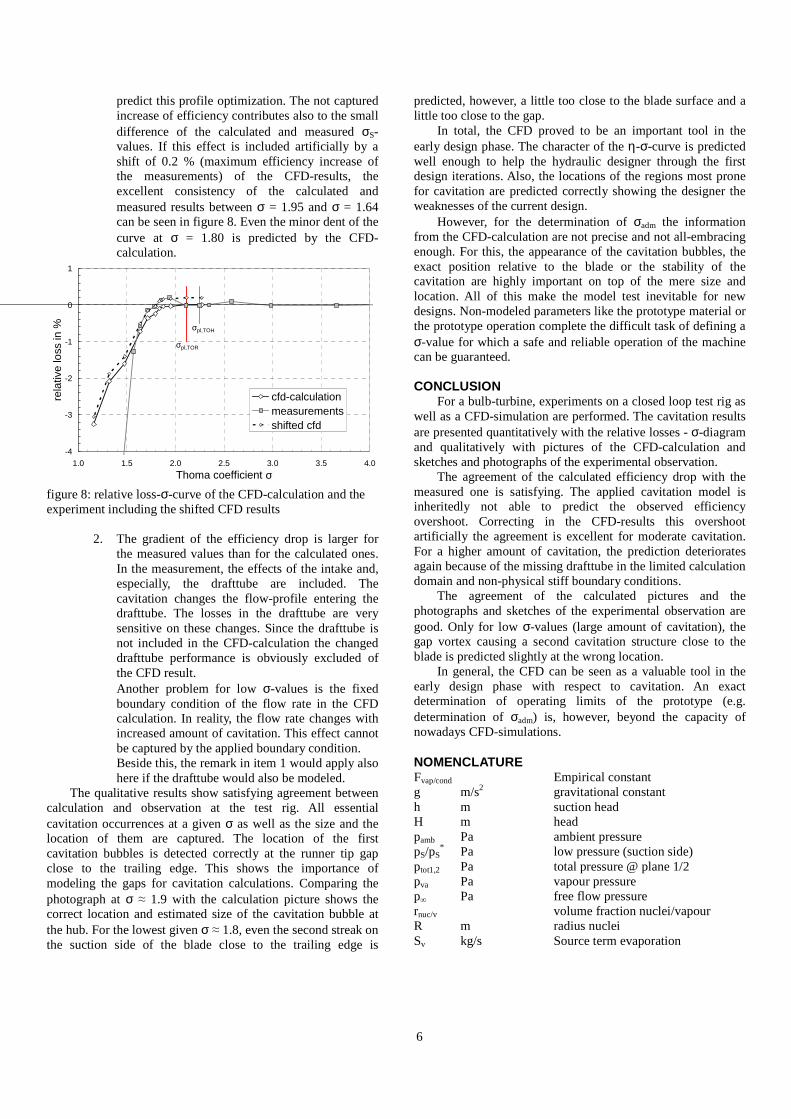
predict this profile optimization. The not captured increase of efficiency contributes also to the small difference of the calculated and measured σS-values. If this effect is included artificially by a shift of 0.2 % (maximum efficiency increase of the measurements) of the CFD-results, the excellent consistency of the calculated and measured results between σ = 1.95 and σ = 1.64 can be seen in figure 8. Even the minor dent of the curve at σ = 1.80 is predicted by the CFD-calculation.

σpl,TOH

σpl,TOR

-4

-3

-2

-1

0

1

1.0 1.5 2.0 2.5 3.0 3.5 4.0

Thoma coefficient σ

rela

tive

loss

in %

cfd-calculationmeasurementsshifted cfd

figure 8: relative loss-σ-curve of the CFD-calculation and the experiment including the shifted CFD results

2. The gradient of the efficiency drop is larger for the measured values than for the calculated ones. In the measurement, the effects of the intake and, especially, the drafttube are included. The cavitation changes the flow-profile entering the drafttube. The losses in the drafttube are very sensitive on these changes. Since the drafttube is not included in the CFD-calculation the changed drafttube performance is obviously excluded of the CFD result. Another problem for low σ-values is the fixed boundary condition of the flow rate in the CFD calculation. In reality, the flow rate changes with increased amount of cavitation. This effect cannot be captured by the applied boundary condition. Beside this, the remark in item 1 would apply also here if the drafttube would also be modeled.

The qualitative results show satisfying agreement between calculation and observation at the test rig. All essential cavitation occurrences at a given σ as well as the size and the location of them are captured. The location of the first cavitation bubbles is detected correctly at the runner tip gap close to the trailing edge. This shows the importance of modeling the gaps for cavitation calculations. Comparing the photograph at σ ≈ 1.9 with the calculation picture shows the correct location and estimated size of the cavitation bubble at the hub. For the lowest given σ ≈ 1.8, even the second streak on the suction side of the blade close to the trailing edge is

predicted, however, a little too close to the blade surface and a little too close to the gap.

In total, the CFD proved to be an important tool in the early design phase. The character of the η-σ-curve is predicted well enough to help the hydraulic designer through the first design iterations. Also, the locations of the regions most prone for cavitation are predicted correctly showing the designer the weaknesses of the current design.

However, for the determination of σadm the information from the CFD-calculation are not precise and not all-embracing enough. For this, the appearance of the cavitation bubbles, the exact position relative to the blade or the stability of the cavitation are highly important on top of the mere size and location. All of this make the model test inevitable for new designs. Non-modeled parameters like the prototype material or the prototype operation complete the difficult task of defining a σ-value for which a safe and reliable operation of the machine can be guaranteed.

CONCLUSION

For a bulb-turbine, experiments on a closed loop test rig as well as a CFD-simulation are performed. The cavitation results are presented quantitatively with the relative losses - σ-diagram and qualitatively with pictures of the CFD-calculation and sketches and photographs of the experimental observation.

The agreement of the calculated efficiency drop with the measured one is satisfying. The applied cavitation model is inheritedly not able to predict the observed efficiency overshoot. Correcting in the CFD-results this overshoot artificially the agreement is excellent for moderate cavitation. For a higher amount of cavitation, the prediction deteriorates again because of the missing drafttube in the limited calculation domain and non-physical stiff boundary conditions.

The agreement of the calculated pictures and the photographs and sketches of the experimental observation are good. Only for low σ-values (large amount of cavitation), the gap vortex causing a second cavitation structure close to the blade is predicted slightly at the wrong location.

In general, the CFD can be seen as a valuable tool in the early design phase with respect to cavitation. An exact determination of operating limits of the prototype (e.g. determination of σadm) is, however, beyond the capacity of nowadays CFD-simulations.

NOMENCLATURE Fvap/cond Empirical constant g m/s2 gravitational constant h m suction head H m head pamb Pa ambient pressure pS/pS

* Pa low pressure (suction side)

ptot1,2 Pa total pressure @ plane 1/2 pva Pa vapour pressure p∞ Pa free flow pressure rnuc/v volume fraction nuclei/vapour R m radius nuclei Sv kg/s Source term evaporation

7

η % efficiency ρ kg/m3 density σ Thoma-coefficient σadm Admissible Thoma-coefficient σpl,TOH Plant Thoma-coefficient, referred to top of hub σpl,TOR Plant Thoma-coefficient, referred to top of runner σS Standard Thoma-coefficient ζabs absolute loss ζrel relative loss

REFERENCES [1] International Electrotechnial Commission, IEC 60193,

Second edition, 1999 [2] Sieber, G; Eichler, O., 1984, Low-pressure circuit test

rig (ND) of the „Brunnenmühle“ Hydraulic Research Laboratory, Voith research and construction, Vol 30

[3] Brand, F., 1984, The measuring equipment of the Hydraulic Research Laboratory “Brunnenmühle“, Voith research and construction, Vol 30

[4] ANSYS INC, Ansys CFX, www.ansys.com/products/fluid-dynamics/cfx/

[5] Stoltz, U., 2007, Berechnung kavitierender Strämungen in Wasserturbinen, Diploma thesis, University of Stuttgart