Torque converter turbine noise and cavitation noise over varying ...

Michigan Technological UniversityDigital Commons @ Michigan

TechDissertations, Master's Theses and Master's Reports- Open Dissertations, Master's Theses and Master's Reports

2012

Torque converter turbine noise and cavitation noiseover varying speed ratioChad Michael WalberMichigan Technological University

Copyright 2012 Chad Michael Walber

Follow this and additional works at: http://digitalcommons.mtu.edu/etds

Part of the Mechanical Engineering Commons

Recommended CitationWalber, Chad Michael, "Torque converter turbine noise and cavitation noise over varying speed ratio", Dissertation, MichiganTechnological University, 2012.http://digitalcommons.mtu.edu/etds/420

http://www.mtu.edu/?utm_source=digitalcommons.mtu.edu%2Fetds%2F420&utm_medium=PDF&utm_campaign=PDFCoverPages

http://www.mtu.edu/?utm_source=digitalcommons.mtu.edu%2Fetds%2F420&utm_medium=PDF&utm_campaign=PDFCoverPages

http://digitalcommons.mtu.edu?utm_source=digitalcommons.mtu.edu%2Fetds%2F420&utm_medium=PDF&utm_campaign=PDFCoverPages

http://digitalcommons.mtu.edu?utm_source=digitalcommons.mtu.edu%2Fetds%2F420&utm_medium=PDF&utm_campaign=PDFCoverPages

http://digitalcommons.mtu.edu/etds?utm_source=digitalcommons.mtu.edu%2Fetds%2F420&utm_medium=PDF&utm_campaign=PDFCoverPages


http://digitalcommons.mtu.edu/etd?utm_source=digitalcommons.mtu.edu%2Fetds%2F420&utm_medium=PDF&utm_campaign=PDFCoverPages


http://network.bepress.com/hgg/discipline/293?utm_source=digitalcommons.mtu.edu%2Fetds%2F420&utm_medium=PDF&utm_campaign=PDFCoverPages

i

TORQUE CONVERTER TURBINE NOISE AND CAVITATION NOISE OVER VARYING SPEED RATIO

By

Chad Michael Walber

A DISSERATION

Submitted in partial fulfillment of the requirements for the degree of

DOCTOR OF PHILOSOPHY

(Mechanical Engineering-Engineering Mechanics)

MICHIGAN TECHNOLOGICAL UNIVERSITY

2012

© 2012 Chad Michael Walber

iii

This dissertation, “Torque Converter Turbine Noise and Cavitation Noise over Varying Speed Ratio,” is hereby approved in partial fulfillment of the requirements for the degree of DOCTOR OF PHILOSOPHY IN MECHANICAL ENGINEERING-ENGINEERING MECHANICS.

Department of Mechanical Engineering-Engineering Mechanics

Signatures:

Dissertation Advisor __________________________________________

Jason R. Blough

Department Chair __________________________________________

William W. Predebon

Date __________________________________________

v

Table of Contents List of Figures .................................................................................................................. vii List of Tables .................................................................................................................. xiii Preface ...............................................................................................................................xv Acknowledgements ....................................................................................................... xvii Abstract ........................................................................................................................... xix Chapter 1 – Literature Review .........................................................................................1 1.1 The Automotive Torque Converter ..............................................................................1 1.2 Cavitation Detection .....................................................................................................5 1.3 Self Excited Vibration ................................................................................................18 1.4 Torque Converter Turbine Noise and Cavitation Noise over Varying Speed Ratio ..26 1.5 References ...................................................................................................................27 Chapter 2 – Predicting Cavitation Desinence in Automotive Torque Converters ....31 2.1 Abstract .......................................................................................................................31 2.2 Introduction .................................................................................................................32 2.3 General Considerations ...............................................................................................35 2.4 Experiment ..................................................................................................................36 2.5 Analysis ......................................................................................................................39 2.6 Results.........................................................................................................................45 2.7 Conclusions.................................................................................................................52 2.8 References ...................................................................................................................53 Chapter 3 – Measuring and Comparing Frequency Response Functions of Torque Converter Turbines Submerged in Transmission Fluid ..............................................55 3.1 Abstract .......................................................................................................................55 3.2 Introduction .................................................................................................................56 3.3 Impact Jigs ..................................................................................................................56 3.4 Ball Bearing Impact ....................................................................................................57 3.5 Impact Rod ..................................................................................................................59 3.6 Comparison of Input Methods ....................................................................................60 3.7 Submerged Modal Testing ..........................................................................................62 3.8 Conclusions.................................................................................................................67 3.9 References ...................................................................................................................68 Chapter 4 – Characterizing Torque Converter Turbine Noise ...................................69 4.1 Abstract .......................................................................................................................69 4.2 Introduction .................................................................................................................70 4.3 Turbine Noise .............................................................................................................71 4.4 Vortex Shedding and Vortex–induced Vibration .......................................................74 4.5 Experimentation ..........................................................................................................78 4.6 Analysis ......................................................................................................................89 4.7 Conclusions.................................................................................................................98

vi

4.8 References .................................................................................................................100 Chapter 5 - Conclusions ................................................................................................101 5.1 Experimental Desinent Cavitation Conclusions .......................................................101 5.2 Turbine Noise Study Conclusions ............................................................................102 5.3 General Automotive Torque Converter Recommendations .....................................102 References .......................................................................................................................105 Appendices ......................................................................................................................111

vii

List of Figures Chapter 1 – Literature Review

Figure 1.1: Cross section of an automotive torque converter; toroidal flow is indicated by the direction of the arrows with no tail. Arrows with tails indicate the normal cooling flow. (1)........................................................................................................................ 2

Figure 1.2: Flow incidence angle across the blades of the stator. (1) ............................... 3

Figure 1.3: Left: Pressure - Volume phase diagram depicting difference between boiling (constant arrow) and cavitation (dashed arrow). Right: Pressure - Temperature phase diagram depicting difference between boiling (constant arrow) and cavitation (dashed arrow). .......................................................................................................................... 6

Figure 1.4: Submarine noise showing transition to noisy operation (cavitation) to depend on depth. (1) ............................................................................................................... 10

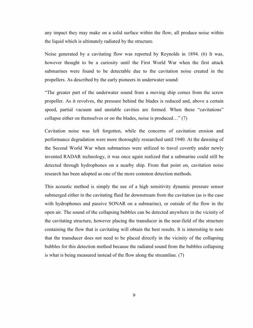
Figure 1.5: Effect of charge pressure on the onset of cavitation for a sample torque converter. (1) .............................................................................................................. 11

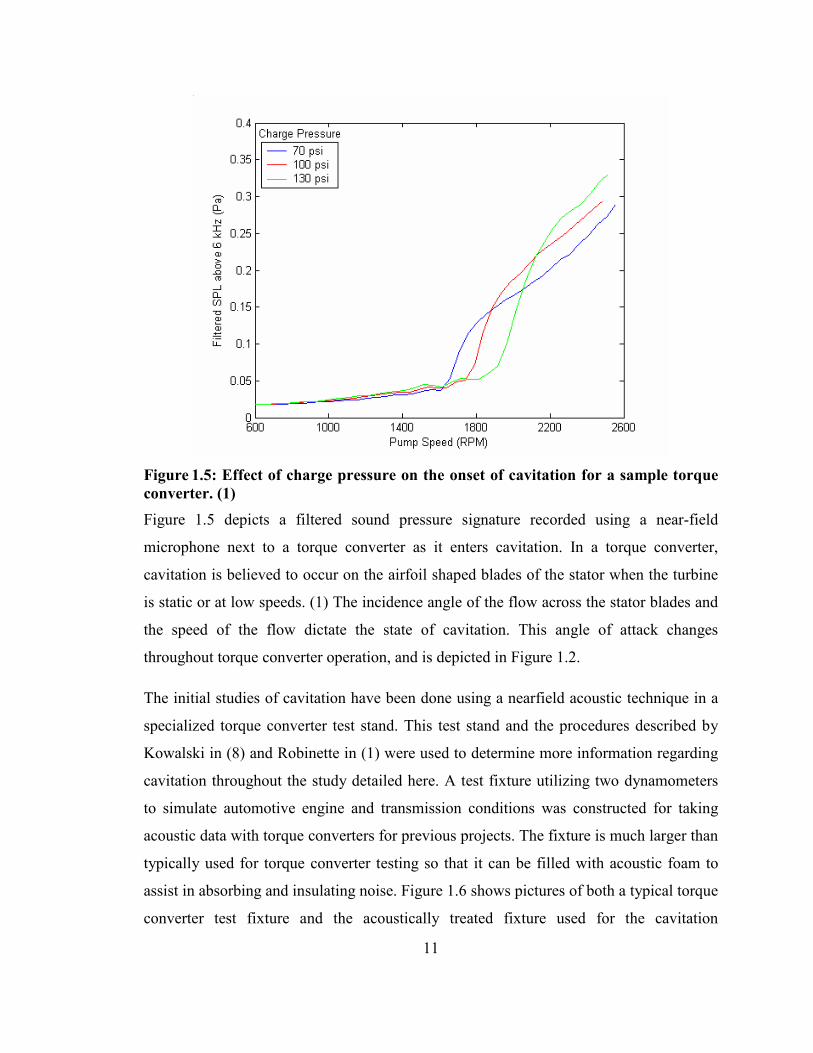
Figure 1.6: Left: Comparison of original torque converter dynamometer test fixture (Red) and acoustic test fixture (Gray). Right: Close up of opened acoustic test stand with acoustic foam. (1)....................................................................................................... 12

Figure 1.7: Microphone placement for torque converter near-field noise measurements.(9) ....................................................................................................... 13

Figure 1.8: Torque converter pump with attached microwave telemetry.(11) ................ 14

Figure 1.9: Signal evolution of the transmitter ring used for microwave telemetry testing.(11) ................................................................................................................. 15

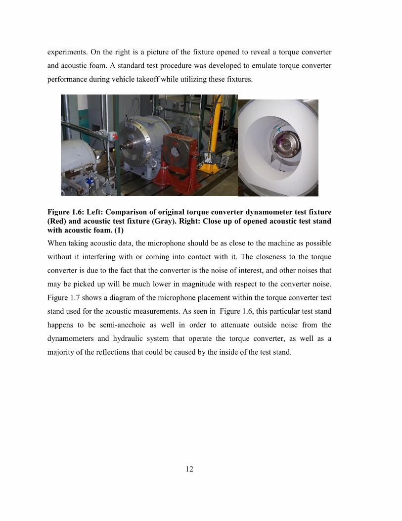
Figure 1.10: Signal evolution for the receiver modules. (11) ......................................... 16

Figure 1.11: Diagram of the mass on a conveyor belt vibration system. ........................ 19

Figure 1.12: Side view of an airfoil in a transverse flow causing a Von Karman Vortex Street. (14).................................................................................................................. 20

Figure 1.13: Strouhal Number for various geometries over Reynolds Number.(15) ...... 22

Figure 1.14: Vortex–induced vibration of a spring–supported, damped circular cylinder. ζ is the damping ratio of the structure. As seen in the two data sets, the lower the damping of the structure, the more motion caused by vortex lock-in, and the longer the vortices remain locked into the motion of the cylinder. (15) ............................... 23

viii

Figure 1.15: Vortex suppression devices attached to cylinders; (a) helical strakes, (b) shroud, (c) axial slats, (d) streamlined fairing, (e) splitter, (f) ribboned cable, (g) pivoted guiding vane, (h) spoiler plates.(15) ............................................................. 24

Figure 1.16: Diagram of flow over a standard fan blade trailing edge, and the trailing edge of a fan made by Noctua with their Vortex–Control Notches. (16) .................. 25

Figure 1.17: Front and side views of a Noctua Fan with Vortex-Control Notches. (16) 25

Chapter 2 – Predicting Cavitation Desinence in Automotive Torque Converters

Figure 2.1: Cross section of an automotive torque converter; toroidal flow is indicated by the direction of the arrows with no tail. Arrows with tails indicate the normal cooling flow (1)....................................................................................................................... 33

Figure 2.2: Flow incidence angle across the blades of the stator (1) .............................. 34

Figure 2.3: Left: Comparison of original torque converter dynamometer test fixture (red) and acoustic test fixture (gray). Right: Close up of opened acoustic test stand with acoustic foam (1)........................................................................................................ 37

Figure 2.4: Example of torque converter speed ratio data plot ....................................... 38

Figure 2.5: Visualization of the algorithm used to determine desinent cavitation in a torque converter ......................................................................................................... 39

Figure 2.6: Left: Schematic of torque converter showing diameter (D) and torus length (Lt) Right: Profile of stator blade depicting maximum thickness (tmax) and chord length (lc) (1) ............................................................................................................. 42

Figure 2.7: Reduction of %RMSE and R2a during stepwise regression for round torus model.......................................................................................................................... 45

Figure 2.8: RS model of desinent cavitation in constant unit input speed family ........... 46

Figure 2.9: RS model of desinent cavitation in torque converters with a round torus shape 47

Figure 2.10: RS model of desinent cavitation in machined from solid torque converters48

Figure 2.11: RS model of desinent cavitation in entire torque converter population ..... 49

Chapter 3 – Measuring and Comparing Frequency Response Functions of Torque Converter Turbines Submerged in Transmission Fluid

Figure 3.1: Close up image of turbine used for testing. .................................................. 56

ix

Figure 3.2: Image of the ball bearing drop jig. The red dot is the laser vibrometer reflecting off of the trailing edge blade of the turbine. The guide tube comes down from the upper right portion of the picture to guide the ball bearing to impact near the laser dot. ..................................................................................................................... 58

Figure 3.3: Photo of impact rod assembly depicting the various parts used. .................. 59

Figure 3.4: Plot comparing FRFs taken using a ball bearing as the excitation and the impact rod. ................................................................................................................. 61

Figure 3.5: Plot comparing the autopower spectra of the "Ideal" impact with the ball bearings with the measured impact with the impact rod............................................ 61

Figure 3.6: FRF plot of driving point on a trailing edge blade. ...................................... 63

Figure 3.7: FRF plot of driving point on edge of shell. .................................................. 64

Figure 3.8: Plot of FRFs of the dry turbine and the wet turbine. The wet turbine has had its frequency scaled in an attempt to remove the additional mass coupling caused by the fluid. ..................................................................................................................... 65

Chapter 4 – Characterizing Torque Converter Turbine Noise

Figure 4.1: Cross section of an automotive torque converter; toroidal flow is indicated by the direction of the arrows with no tail. Arrows with tails indicate the normal cooling flow (1)....................................................................................................................... 70

Figure 4.2: Nearfield acoustic measurement of automotive torque converter equipped with an un-notched trailing edge turbine (Top) and a notched trailing edge turbine (Bottom) during simulated vehicle launch on dynamometer with an input torque of 350Nm. The area circled in white denotes the Turbine noise. ................................... 73

Figure 4.3: Comparison of noise from an un-notched “Noisy” turbine and a notched quiet turbine during simulated vehicle launch with an input torque of 350Nm. ................ 74

Figure 4.4: Side view of an airfoil in a transverse flow causing a Von Karman Vortex Street.(3)..................................................................................................................... 75

Figure 4.5: Strouhal Number for various geometries over Reynolds Number. (4) ......... 76

Figure 4.6: Vortex–induced vibration of a spring–supported, damped circular cylinder. ζ is the damping ratio of the structure. As seen in the two data sets, the lower the damping of the structure, the more motion caused by vortex lock-in, and the longer the vortices remain locked into the motion of the cylinder. (4) ................................. 77

Figure 4.7: Diagram of flow over a standard fan blade trailing edge, and the trailing edge of a fan made by Noctua with their Vortex–Control Notches. (5)............................. 78

x

Figure 4.8: Photographs of an un-notched turbine that exhibits the “Turbine Noise” (Left) and a notched turbine (Right). ................................................................................... 79

Figure 4.9: Comparison of autopower response of turbines known to be noisy during operation (Both un-notched turbines) to those that were known to be quiet during operation (MFS and both notched turbines) in air. .................................................... 80

Figure 4.10: Comparison of frequency response functions of a reference point on the hub of the un-notched turbine of a noisy turbine with four trailing edge blades tested in air. 81

Figure 4.11: Comparison of frequency response functions of a reference point on the hub of the un-notched turbine of a noisy turbine with four trailing edge blades zoomed in to the natural frequencies thought to be associated with the trailing edge blades tested in air. .......................................................................................................................... 81

Figure 4.12: Comparison of frequency response functions of a reference point on the hub of the un-notched turbine of a noisy turbine with four trailing edge blades tested in ATF. ........................................................................................................................... 83

Figure 4.13: Left: Comparison of original torque converter dynamometer test fixture (Red) and acoustic test fixture (Gray). Right: Close up of opened acoustic test stand with acoustic foam. (1) .............................................................................................. 84

Figure 4.14: Comparison of Torque Converter turbine noise at various input torque steps. 85

Figure 4.15: Photographs of un-notched turbine trailing edge with dummy transducers (Left) and wires combined with dummy transducers (Right). ................................... 86

Figure 4.16: SPL plot comparing test alterations to turbine trailing edge. ..................... 87

Figure 4.17: Polycarbonate Extension Ring used to facilitate microwave telemetry measurements. ............................................................................................................ 88

Figure 4.18: Cross–section of assembled telemetry torque converter. The polycarbonate extension ring and the microwave transmitter are annotated. .................................... 88

Figure 4.19: Spectrogram of trailing edge accelerometer measurement on automotive torque converters equipped with an un-notched (Top) and notched (Bottom) trailing edge turbine during simulated vehicle launch with an input torque of 350Nm. ........ 90

Figure 4.20: Spectrogram of trailing edge pressure measurement on automotive torque converter equipped with an un-notched (Top) and notched (Bottom) trailing edge turbine during simulated vehicle launch with an input torque of 350Nm. ................ 92

Figure 4.21: Spectrogram of trailing edge strain gage measurement on automotive torque converter equipped with an un-notched (Top) and notched (Bottom) trailing edge turbine during simulated vehicle launch with an input torque of 350Nm. ................ 93

xi

Figure 4.22: Estimated turbine exit mean velocity at each tested input torque over speed ratio. ........................................................................................................................... 94

Figure 4.23: Plots of estimated vortex frequency (Top) and filtered sound pressure level (Bottom) over speed ratio. The noise data was taken during simulated vehicle launch testing on dynamometer with an input torque of 350Nm. The vortex frequency was calculated using the turbine exit velocity curve for 350Nm, a trailing edge thickness of .6mm, and a Strouhal Number of .28 over the entire test. ..................................... 95

Figure 4.24: SPL plot comparing noise level in converters with different stator and pump combinations. Each of the tests shown was run at 300 Nm input torque. ................. 97

Figure 4.25: Color maps comparing a stock turbine noise (Top) with the same turbine after machining the trailing edge thinner (Bottom), both tests at 350 Nm input torque 98

Appendix B – Submerged Turbine Modal Analysis

Figure B.1: Comparison of autopower response of turbines known to be noisy during operation (Both unnotched turbines) to those that were known to be quiet during operation (MFS and both notched turbines) in air. .................................................. 126

Figure B.2: Comparison of frequency response functions of a reference point on the hub of the unnotched turbine of a noisy turbine with four trailing edge blades tested in air. 127

Figure B.3: Comparison of frequency response functions of a reference point on the hub of the unnotched turbine of a noisy turbine with four trailing edge blades zoomed in to the natural frequencies thought to be associated with the trailing edge blades tested in air. ........................................................................................................................ 127

Figure B.4: Comparison of frequency response functions of a reference point on the hub of the unnotched turbine of a noisy turbine with four trailing edge blades tested in ATF. ......................................................................................................................... 129

Figure B.5: Shell breathing mode shape of turbine in air (Left column) and in ATF (Right column) shown at the opposite motion extremes (Top and bottom). MAC=72% ............................................................................................................... 130

Figure B.6: Three lobed mode shape of turbine in air (Left column) and in ATF (Right column) shown at the opposite motion extremes (Top and bottom). MAC=69% ... 130

xiii

List of Tables Chapter 2 - Predicting Cavitation Desinence in Automotive Torque Converters

Table 2.1: Dimensionless Parameters used in Speed Ratio Correlation ............................40

Table 2.2: RS Models by Torque Converter Population minus Regression Coefficients .50

Chapter 3 – Measuring and Comparing Frequency Response Functions of Torque Converter Turbines Submerged in Transmission Fluid

Table 3.1: This table is a comparison of the first six natural frequencies that appear in the FRFs of the driving point on the shell of the turbine. ..................................................63

xv

Preface The content of this dissertation includes several full-text journal articles. A description of

the contribution by the author of this dissertation to each article follows.

In all three of the papers included in this dissertation:

• Predicting Cavitation Desinence in Automotive Torque Converters

• Measuring and Comparing Frequency Response Functions of Torque

Converter Turbines Submerged in Transmission Fluid

• Characterizing Torque Converter Turbine Noise

All of the experimentation, data analysis, dimensionless correlations, and background

research was performed by the author of this dissertation. The coauthors of these papers

supplied valued insight and experience into the phenomena discussed.

xvii

Acknowledgements Very few things in the world can be accomplished without the assistance of at least one other person. I have been blessed in my life to have many people there for me as an emotional support system, a helping hand in the work shop, a sounding board for my new ideas, or just a dear friend to help me relax. There is no way I can thank everyone for what they have done for me, but I hope that this is a good start…

First, I need to thank my parents, without whom I would not be here, both in a sense that I would not exist, and in that I would not have achieved so much at this point in my life without them. They let me be my own person throughout my life, with a couple pushes here and there to keep me going down the road I’m on. I love both of you guys very much.

I was not blessed with siblings, but I was given something I consider to be better, my best friends. Most count themselves lucky to have one best friend; I have five: Tyler Schwochert, Josh Fogarty, Cory Basler, Scott Gross, and Chris Rice. You guys have always been there for me. You were always honest, wise, and yet caring. I take a little piece of each of you with me wherever I go, and because of each of you I am a better man.

I thank my entire committee, but especially Jason Blough and Chuck VanKarsen, both of whom I would not be fulfilling this task without. You guys dared me to do better, and because of that I have achieved this great task. I thank Ashok Ambardar for teaching me that knowing something is not enough, that understanding is the key. I thank Chris Passerello for teaching me that although it can be arduous and time consuming, dynamics truly is the most fun you can have with a piece of chalk. All those who have been in the lab working with me also need thanks, for your support, as well as for the comic relief. Final thanks go out to VK, Keske, and Brandon, who have all been both coworkers and dear friends.

I thank all of the folks at General Motors, most especially Jean Schweitzer, for the fiscal assistance and guidance throughout this project. I know times were tough there for a while, but you stood by through it all and help make this all of the needs of this project come to fruition.

Lastly I would like to thank the many others who have contributed to this task and helped to make my journey fantastic. This includes all of the MEEM Staff, the people at IR Telemetrics, and the many other friends, family, and coworkers that I couldn’t list here. Thank you all.

xix

Abstract These investigations will discuss the operational noise caused by automotive torque

converters during speed ratio operation. Two specific cases of torque converter noise will

be studied; cavitation, and a monotonic turbine induced noise. Cavitation occurs at or

near stall, or zero turbine speed. The bubbles produced due to the extreme torques at low

speed ratio operation, upon collapse, may cause a broadband noise that is unwanted by

those who are occupying the vehicle as other portions of the vehicle drive train improve

acoustically. Turbine induced noise, which occurs at high engine torque at around 0.5

speed ratio, is a narrow-band phenomenon that is audible to vehicle occupants currently.

The solution to the turbine induced noise is known, however this study is to gain a better

understanding of the mechanics behind this occurrence.

The automated torque converter dynamometer test cell was utilized in these experiments

to determine the effect of torque converter design parameters on the offset of cavitation

and to employ the use a microwave telemetry system to directly measure pressures and

structural motion on the turbine. Nearfield acoustics were used as a detection method for

all phenomena while using a standardized speed ratio sweep test. Changes in filtered

sound pressure levels enabled the ability to detect cavitation desinence. This, in turn, was

utilized to determine the effects of various torque converter design parameters, including

diameter, torus dimensions, and pump and stator blade designs on cavitation. The on

turbine pressures and motion measured with the microwave telemetry were used to

understand better the effects of a notched trailing edge turbine blade on the turbine

induced noise.

1

Chapter 1 – Literature Review

This chapter is the review of the important literature with regards to automotive torque

converters, experimental cavitation detection, and Von Karman vortex shedding.

1.1 The Automotive Torque Converter Several definitions need to be made to further discuss the automotive torque converter

which is a member of a much larger family of machines called turbomachines.

Turbomachines are a class of devices that utilize continuously flowing fluids to transfer

energy to or from one or more rows of rotating blades. A subset of turbomachines is the

pump in which energy is imparted to a working fluid; this subset includes propellers,

impellors, fans, and compressors. Turbines are turbomachines that receive and utilize the

energy of a fluid in motion. Common turbines are found in hydroelectric power

generators, flow meters, torque converters, and windmills. Flow through these machines

can be axial, which is parallel to the axis of rotation, radial, which is perpendicular to the

axis of rotation, or a combination of these. Lastly, turbomachines can be classified by the

extent which the fluid affects the machine. Open machines have a control volume that is

theoretically infinite, such as wind turbines and propellers. Closed machines are those

such as pumps, water turbines, and torque converters which have a finite control volume.

In general, open machines are more difficult to test and analyze without making a large

number of assumptions, therefore they will not be further discussed in this paper.

The automotive torque converter is the powertrain component that multiplies engine

torque, acts to augment a much smaller flywheel than what is found in manual

transmission applications, and allows the engine to idle. Modern automotive torque

converters are made up of three elements, a mixed flow pump and turbine, and an axial

flow stator. Figure 1.1 is a basic schematic of a torque converter, including arrows

showing the direction of the toroidal flow induced during operation. Maximum efficiency

is achieved during high speed ratio operation while maximum torque multiplication is

attained at stall, or turbine speed equal to zero. Speed ratio (SR) is defined as the ratio of

the turbine speed over the pump speed.

2

Figure 1.1: Cross section of an automotive torque converter; toroidal flow is indicated by the direction of the arrows with no tail. Arrows with tails indicate the normal cooling flow. (1) In the basic operation of a torque converter, the pump is driven by the engine through

connection of the engine crankshaft and flexplate to the cover of the torque converter.

Rotation of the pump imparts angular momentum onto the automatic transmission fluid

(ATF). The fluid flows from the inner radius of the pump flow path to the outer radius,

and is directed into the turbine. The turbine turns the flow and directs it radially inward to

the stator which guides the flow back into the pump. Fluid is redirected as it flows

through each of the bladed elements shown in Figure 1.1. The change in the angular

momentum of the fluid across a particular element results in a torque being applied to the

shaft attached to that element. Therefore, angular momentum change of the fluid across

the turbine imparts a torque on the turbine shaft which is the input shaft to the automatic

transmission. The stator, which is designed to redirect the flow from the turbine into a

favorable angle with regards to pump operation, creates another change in the fluid’s

angular momentum, creating another torque across the stator. Since the stator is fixed via

a one-way clutch to a static shaft attached to the transmission housing, this torque is

absorbed. It is the torque being absorbed by the stator that creates torque multiplication.

Equation 1 shows the equation created via free body analysis of the three elements of the

torque converter. The torque multiplication factor calculated by the torque ratio (TR) of

3

the turbine over the pump is the performance characteristic that helps the vehicle

accelerate from a stop.

StatorPumpturbine TTT += (1)

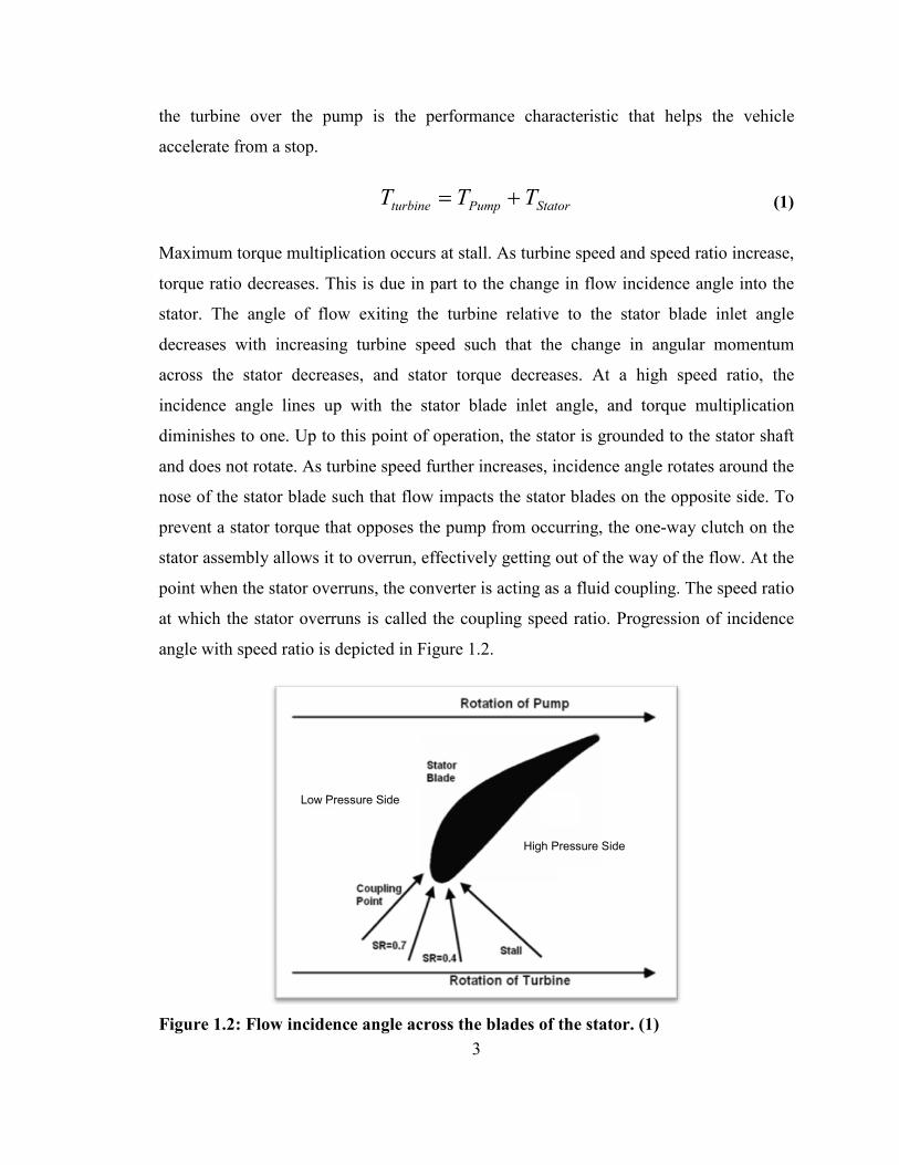
Maximum torque multiplication occurs at stall. As turbine speed and speed ratio increase,

torque ratio decreases. This is due in part to the change in flow incidence angle into the

stator. The angle of flow exiting the turbine relative to the stator blade inlet angle

decreases with increasing turbine speed such that the change in angular momentum

across the stator decreases, and stator torque decreases. At a high speed ratio, the

incidence angle lines up with the stator blade inlet angle, and torque multiplication

diminishes to one. Up to this point of operation, the stator is grounded to the stator shaft

and does not rotate. As turbine speed further increases, incidence angle rotates around the

nose of the stator blade such that flow impacts the stator blades on the opposite side. To

prevent a stator torque that opposes the pump from occurring, the one-way clutch on the

stator assembly allows it to overrun, effectively getting out of the way of the flow. At the

point when the stator overruns, the converter is acting as a fluid coupling. The speed ratio

at which the stator overruns is called the coupling speed ratio. Progression of incidence

angle with speed ratio is depicted in Figure 1.2.

Figure 1.2: Flow incidence angle across the blades of the stator. (1)

Low Pressure Side

High Pressure Side

4

Torque converters need temperature control to prevent overheating of the ATF. Under

practical operation, a converter functions at less than unit efficiency, and all power loss is

converted to heat within the working fluid. The automatic transmission pump forces a

continuous flow of cooling fluid through the torque converter. ATF flows into the

converter between the cover and the clutch, and then into the outer torus region between

the pump and the turbine where it is integrated into the toroidal flow. The direction of

this flow is indicated in Figure 1.1 by the arrows with tails. The hotter fluid is evacuated

from the converter to the vehicle cooling system. A second function of the transmission

pump is to control the level of pressure in the torque converter to suppress cavitation. The

flow into the converter is called charge pressure, and the flow out is called back pressure.

When the torque converter is operating at high speed ratios, a clutch can be engaged to

create a direct shaft connection between the engine and transmission to bypass the

hydrodynamic inefficiency of the torque converter. The clutch is engaged by reversing

the cooling flow to raise the pressure behind the clutch assembly and lower the pressure

between the cover and clutch. This pushes the pressure plate of the clutch toward the

cover of the converter, and friction material on the clutch plate engages with the surface

of the cover. Apply pressure is regulated to create either a full lock between the cover and

clutch, or a controlled speed slip.

In torque converter mode, individual element torques are created from the change in

angular momentum flux across an element from inlet to outlet. The torque is a function of

the local static pressure times the radius integrated over the entire surface of each blade.

A greater pressure differential across a blade proportionally increases the individual

element torque. Consequently, at some large element torque, the pressure on the low

pressure side of a blade can drop to below the vapor pressure of the fluid, and the

nucleation of cavitation bubbles may occur.

The effect of cavitation on performance is dependent on whether sustained cavitation is

reached. Incipient cavitation can occur at stall and dissipate before it is of any

consequence. But if a high level of element torque is sustained for a long duration, the

heavy cavitation will result in large vapor regions that displace the working fluid, affect

5

performance, and possibly cause damage when cavitation bubbles collapse. Furthermore,

collapsing bubbles cause a broadband noise that may affect the overall sound quality of

the vehicle. (1) Advanced cavitation causes a decrease in individual element torques,

which alters the relationship between speed and torque for the converter.

1.2 Cavitation Detection Cavitation is the formation and collapse of voids within a pure liquid due to rapid high

magnitude pressure fluctuation. These voids are the gaseous phase of the operating fluid.

The difference between cavitating and boiling lies in the method by which the phase

change occurs. Boiling is caused by changing the temperature of the liquid to the boiling

temperature while the pressure is kept fairly constant, while cavitation is caused by

keeping the temperature fairly constant while lowering the pressure below the vapor

pressure of the fluid and thereby causing bubbles of gas to form. These are outlined better

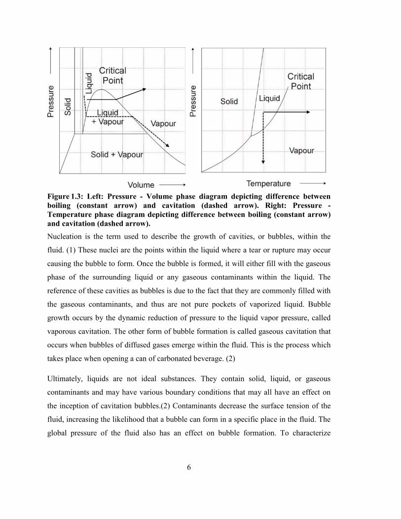
in Figure 1.3. In ideal liquids these phase diagrams accurately represent the pressure at

which vapor cavities form. In the P-V diagram, following an isotherm across the

liquid+vapor region is a cavitation process. The difference between boiling and cavitation

is even more evident in the P-T diagram, where crossing the saturated vapor line

horizontally, that is maintaining constant pressure and increasing temperature, is boiling

and crossing it vertically, or dynamically decreasing pressure while somehow

maintaining temperature, is cavitation.

6

Figure 1.3: Left: Pressure - Volume phase diagram depicting difference between boiling (constant arrow) and cavitation (dashed arrow). Right: Pressure - Temperature phase diagram depicting difference between boiling (constant arrow) and cavitation (dashed arrow). Nucleation is the term used to describe the growth of cavities, or bubbles, within the

fluid. (1) These nuclei are the points within the liquid where a tear or rupture may occur

causing the bubble to form. Once the bubble is formed, it will either fill with the gaseous

phase of the surrounding liquid or any gaseous contaminants within the liquid. The

reference of these cavities as bubbles is due to the fact that they are commonly filled with

the gaseous contaminants, and thus are not pure pockets of vaporized liquid. Bubble

growth occurs by the dynamic reduction of pressure to the liquid vapor pressure, called

vaporous cavitation. The other form of bubble formation is called gaseous cavitation that

occurs when bubbles of diffused gases emerge within the fluid. This is the process which

takes place when opening a can of carbonated beverage. (2)

Ultimately, liquids are not ideal substances. They contain solid, liquid, or gaseous

contaminants and may have various boundary conditions that may all have an effect on

the inception of cavitation bubbles.(2) Contaminants decrease the surface tension of the

fluid, increasing the likelihood that a bubble can form in a specific place in the fluid. The

global pressure of the fluid also has an effect on bubble formation. To characterize

7

cavitation, the cavitation number, shown in Equation 2, classifies whether cavitation is

occurring.

2

2

1 V

pp vaporlocallocal

ρσ

−= (2)

In this equation plocal is the local pressure of the liquid, pvapor is the vapor pressure of the

bulk liquid including contaminants, ρ is the density of the fluid, and V is the freestream

velocity of the fluid. When a fluid is forced to move around solid boundaries pressure

drops are caused. The nuclei that come close to those pressure drops, if they are sufficient

to break the tensile strength of said liquid, will grow into a bubble and continue on to

flow with the liquid portion of the fluid. These bubbles will keep growing and eventually

collapsing as either the local liquid pressure increases, or the temperature drops thus

increasing the tensile strength of the liquid again. Ideally, once bubbles are forming and

the liquid pressure reaches the vapor pressure, Equation 2 should equal zero.

Experimental results have show with pressure taps at the point of cavitation inception that

liquid pressure does indeed follow this phenomenon.(2)

Experimental Cavitation Detection – Cavitation was first discovered in turbomachines

as a drop in element torque which caused inefficiency in the system.(4) Since that

discovery, it has been found that cavitation also causes wideband noise, material damage,

and unwanted vibration. Several applications within chemical engineering have

determined that the phase change induced by a cavitated flow can have ill effects on

certain chemical reactions.(5)

For all of these reasons, it is vital that whenever advanced cavitation occurs that it is

brought under control. Many of the previously mentioned experiments in cavitation

occurred in water tunnels to simply determine the parameters that cause cavitation to

occur. These were all designed to make the phenomenon easily measureable. Real life

applications can be much more difficult, especially when the flow under study has

already been established within a machine. Furthermore, as turbomachines can be

8

difficult to model in their own right, it can be even more difficult to get measurement

devices in a location to accurately measure if cavitation is occurring. Rotating blades,

solid housings, high pressures, and hot fluids can all prevent an experimentalist from

getting the measurements needed in order to determine the cavitation behavior of a fluid.

Fortunately, there are many specific phenomena that can easily be measured from the

inception of cavitation within a flow. The collapsing of these bubbles along with the

impact they make upon solid boundaries causes a broadband noise to be emitted from the

liquid. Furthermore, the bubbles can be visually seen forming and collapsing within the

liquid. Most invasively, pressure transducers within the flow can also be used at and

along the path over which cavitation is thought to be occurring. In this last case,

cavitation is detected by a wideband fluctuation of the pressure within the flow.

However, placing actual transducers near or on the machine can cause a change in the

cavitating flow. The rougher a surface is, the more likely the lower the liquid tensile

strength and therefore any aberration on a surface can act as a nucleation point, causing

an otherwise smooth surface to begin cavitation in the liquid before it normally would.

Image acquisition may require a sight glass or a Plexiglas pipe be installed near the

machine. This would be to great cost, and would ultimately have an effect on the flow

being studied. Near-field acoustic acquisition is a completely noninvasive technique

utilizing microphones near the cavitation source to detect broadband noise. Acoustic

detection is the most cost efficient means of determining the presence of cavitation, and

therefore will be discussed next.

Acoustic Detection – One of the signatures of a cavitating flow is the noise produced. As

the local pressures within a flow vary, bubbles grow, shrink, and ultimately collapse once

they have reached a location in the flow where the local pressure is greater than the

tensile strength of the liquid. Furthermore, the collapse of bubbles creates more

nucleation sites within the liquid. These additional nuclei are the reason why liquid

history is important when attempting to analytically determine the point of cavitation. If a

liquid has been previously cavitated the collapsed bubbles of a previously cavitated liquid

make it more prone to cavitation additional times. The collapse of the bubbles, along with

9

any impact they may make on a solid surface within the flow, all produce noise within

the liquid which is ultimately radiated by the structure.

Noise generated by a cavitating flow was reported by Reynolds in 1894. (6) It was,

however thought to be a curiosity until the First World War when the first attack

submarines were found to be detectable due to the cavitation noise created in the

propellers. As described by the early pioneers in underwater sound:

“The greater part of the underwater sound from a moving ship comes from the screw

propeller. As it revolves, the pressure behind the blades is reduced and, above a certain

speed, partial vacuum and unstable cavities are formed. When these “cavitations”

collapse either on themselves or on the blades, noise is produced…” (7)

Cavitation noise was left forgotten, while the concerns of cavitation erosion and

performance degradation were more thoroughly researched until 1940. At the dawning of

the Second World War when submarines were utilized to travel covertly under newly

invented RADAR technology, it was once again realized that a submarine could still be

detected through hydrophones on a nearby ship. From that point on, cavitation noise

research has been adopted as one of the more common detection methods.

This acoustic method is simply the use of a high sensitivity dynamic pressure sensor

submerged either in the cavitating fluid far downstream from the cavitation (as is the case

with hydrophones and passive SONAR on a submarine), or outside of the flow in the

open air. The sound of the collapsing bubbles can be detected anywhere in the vicinity of

the cavitating structure, however placing the transducer in the near-field of the structure

containing the flow that is cavitating will obtain the best results. It is interesting to note

that the transducer does not need to be placed directly in the vicinity of the collapsing

bubbles for this detection method because the radiated sound from the bubbles collapsing

is what is being measured instead of the flow along the streamline. (7)

10

Figure 1.4: Submarine noise showing transition to noisy operation (cavitation) to depend on depth. (1) The results of acoustic cavitation detection have a well established correlation. Figure 1.4

shows the time averaged noise level over time of a submarine in the water. As the depth

of the boat increases (analogous to the controlled pressure of the fluid of operation), the

speed required to increase the noise level also increases. As this noise level is a direct

correlation of the number of bubbles collapsing in the flow, it also correlates with

Equation 2, which is that it will take more work to create a bubble if the liquid’s

controlled pressure is increased. The sudden increase in the slope of the noise level

dictates the inception of cavitation. At deeper depths, the rapid and sudden slope change

does not occur, which indicates that either cavitation may not be occurring, the noise

detected is from another point in the machine, or that the amount of cavitation occurring

is very insignificant. (7)

11

Figure 1.5: Effect of charge pressure on the onset of cavitation for a sample torque converter. (1) Figure 1.5 depicts a filtered sound pressure signature recorded using a near-field

microphone next to a torque converter as it enters cavitation. In a torque converter,

cavitation is believed to occur on the airfoil shaped blades of the stator when the turbine

is static or at low speeds. (1) The incidence angle of the flow across the stator blades and

the speed of the flow dictate the state of cavitation. This angle of attack changes

throughout torque converter operation, and is depicted in Figure 1.2.

The initial studies of cavitation have been done using a nearfield acoustic technique in a

specialized torque converter test stand. This test stand and the procedures described by

Kowalski in (8) and Robinette in (1) were used to determine more information regarding

cavitation throughout the study detailed here. A test fixture utilizing two dynamometers

to simulate automotive engine and transmission conditions was constructed for taking

acoustic data with torque converters for previous projects. The fixture is much larger than

typically used for torque converter testing so that it can be filled with acoustic foam to

assist in absorbing and insulating noise. Figure 1.6 shows pictures of both a typical torque

converter test fixture and the acoustically treated fixture used for the cavitation

12

experiments. On the right is a picture of the fixture opened to reveal a torque converter

and acoustic foam. A standard test procedure was developed to emulate torque converter

performance during vehicle takeoff while utilizing these fixtures.

Figure 1.6: Left: Comparison of original torque converter dynamometer test fixture (Red) and acoustic test fixture (Gray). Right: Close up of opened acoustic test stand with acoustic foam. (1) When taking acoustic data, the microphone should be as close to the machine as possible

without it interfering with or coming into contact with it. The closeness to the torque

converter is due to the fact that the converter is the noise of interest, and other noises that

may be picked up will be much lower in magnitude with respect to the converter noise.

Figure 1.7 shows a diagram of the microphone placement within the torque converter test

stand used for the acoustic measurements. As seen in Figure 1.6, this particular test stand

happens to be semi-anechoic as well in order to attenuate outside noise from the

dynamometers and hydraulic system that operate the torque converter, as well as a

majority of the reflections that could be caused by the inside of the test stand.

13

Figure 1.7: Microphone placement for torque converter near-field noise measurements.(9) Using the noise level as an indicator function is a common means of determining the

onset of cavitation; however it is not without its shortcomings. Cavitation is a broadband

noise, so care needs to be taken to be sure that what is being measured is indeed

cavitation and not some other broadband noise source. When making in-situ

measurements or those where there are other noise sources close a high pass filter can

remove a great deal of surrounding machine noise so that the high frequencies of the

cavitation noise can be detected.(10)

Pressure Telemetry Measurements – As technology evolves, it becomes easier to apply

transducers to complex systems and even systems that are rotating within static surfaces

such as turbomachines. This wireless telemetry allows for pressure, strain, and

acceleration measurements to be taken right at the tip of a rotating airfoil. A picture of a

torque converter pump with attached microwave telemetry is shown in Figure 1.8. This

particular pump was outfitted with pressure taps that measured the pressure fluctuations

of a torque converter stator while it was cavitating.(4)

Torque Converter

Microphone

14

Figure 1.8: Torque converter pump with attached microwave telemetry.(11) The principle by which the telemetry works is called a double frequency modulation

(FM) technique. This is identical to radio transmission, with the exception that the

electromagnetic frequencies for transmission are in the microwave realm which is the 1

to 300 GHz range. Any transducer type may be used provided they can be adapted to

interface with the telemetry system.

First the conditioned signal is converted to a one-volt amplitude square wave with a

fundamental frequency in the range of frequencies of 10 and 60 kHz corresponding to 0

and 10 volts respectively. This signal is modulated with a final 2.4 GHz band carrier

wave. Two frequencies in this band are used as signal references for high and low

voltages respectively from the previous step. This final 2.4 GHz signal is what is then

transmitted. The signal evolution diagram of these steps is shown in Figure 1.9.

15

Figure 1.9: Signal evolution of the transmitter ring used for microwave telemetry testing.(11) A microwave antenna can be set up for machines that rotate external to the flow, and the

wiring can simply be machined into the part. If the part is spinning within a metal

housing, a special cover made of Lexan or some other dielectric material may need to be

constructed in order to allow the microwaves to pass to the receiver outside of the flow

being measured.

In the case of the Zeng project (4), antennas placed inside the test stand gather the signals

being transmitted and send them down a wire to an amplifier. At this point all signals

from all transmitters, as well as all outside noise sources which can include car radio,

wifi, and cell phone signals, are included in the signal. Once the amplifier sends the

signal on to the receiver, all data from everything except the specific channel of interest

are filtered out, leaving an amplitude-varied version of the signal transmitted by the

corresponding transmitter.

This signal is demodulated into the square wave, which should theoretically be identical

to the square wave created in the transmitter. The square wave goes through a frequency

to voltage conversion (another demodulation process) and is low-pass filtered. This final

signal should be nearly identical to the original conditioned signal, and is fed into the

high speed data acquisition system. The signal evolution of this portion of the telemetry

scheme is shown in Figure 1.10.

16

Figure 1.10: Signal evolution for the receiver modules. (11) Another scheme that is currently being tested is an inductive transmission scheme.(11) In

this method, two sets of coils are set rotating very close to each other. The primary coil

attached to the telemetry is then energized with an electric current that is operating at a

set carrier frequency and contains the data encoded by the telemetry inside the machine.

Similar to an electric power transformer, the varying electric field creates a magnetic

field which excites the second coil causing it to pick up the signal being transmitted. To

enhance transmission, iron cores are used to refocus the magnetic field from around the

primary coil to around the secondary.

Using telemetry coupled with fluctuating pressure measurements is, experimentally, one

of the best methods that can be used to determine if cavitation is occurring at a specific

place within a flow. A pressure measurement can be taken at a very specific place on the

blades of a turbomachine. The pressure measurement can then be entered into Equation 2

to give an experimentally determined cavitation number. If dynamic transducers are used,

the violent pressure fluctuations associated with bubble collapse can even be measured

and used as an indicator of the onset of cavitation.

However, telemetry has its disadvantages. Due to the expense associated with the

modifications required to be made on the rotating device, including all of the electronic

17

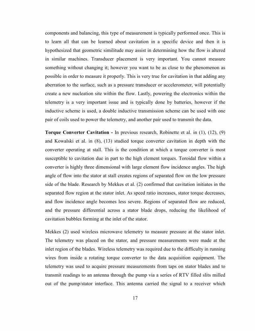
components and balancing, this type of measurement is typically performed once. This is

to learn all that can be learned about cavitation in a specific device and then it is

hypothesized that geometric similitude may assist in determining how the flow is altered

in similar machines. Transducer placement is very important. You cannot measure

something without changing it; however you want to be as close to the phenomenon as

possible in order to measure it properly. This is very true for cavitation in that adding any

aberration to the surface, such as a pressure transducer or accelerometer, will potentially

create a new nucleation site within the flow. Lastly, powering the electronics within the

telemetry is a very important issue and is typically done by batteries, however if the

inductive scheme is used, a double inductive transmission scheme can be used with one

pair of coils used to power the telemetry, and another pair used to transmit the data.

Torque Converter Cavitation - In previous research, Robinette et al. in (1), (12), (9)

and Kowalski et al. in (8), (13) studied torque converter cavitation in depth with the

converter operating at stall. This is the condition at which a torque converter is most

susceptible to cavitation due in part to the high element torques. Toroidal flow within a

converter is highly three dimensional with large element flow incidence angles. The high

angle of flow into the stator at stall creates regions of separated flow on the low pressure

side of the blade. Research by Mekkes et al. (2) confirmed that cavitation initiates in the

separated flow region at the stator inlet. As speed ratio increases, stator torque decreases,

and flow incidence angle becomes less severe. Regions of separated flow are reduced,

and the pressure differential across a stator blade drops, reducing the likelihood of

cavitation bubbles forming at the inlet of the stator.

Mekkes (2) used wireless microwave telemetry to measure pressure at the stator inlet.

The telemetry was placed on the stator, and pressure measurements were made at the

inlet region of the blades. Wireless telemetry was required due to the difficulty in running

wires from inside a rotating torque converter to the data acquisition equipment. The

telemetry was used to acquire pressure measurements from taps on stator blades and to

transmit readings to an antenna through the pump via a series of RTV filled slits milled

out of the pump/stator interface. This antenna carried the signal to a receiver which

18

converted it back to the raw data for a data acquisition system. A method was developed

by Kowalski (8) that uses nearfield acoustic measurements to accurately detect cavitation

without requiring wireless telemetry. In this way, a large population of torque converters

can be tested for cavitation without the time and expense needed to create microwave

instrumented torque converters for each blade design of interest. Robinette et al. (1) and

(9) used the acoustic method to determine incipient cavitation at stall for a population of

torque converters with a wide range of sizes and blade geometries. A correlation was

formulated based on operating conditions and converter geometry to estimate the point of

incipient cavitation during stall.

1.3 Self Excited Vibration The study of vibratory motion has three major sub topics. Free vibration is when a system

is taken out of rest for a short time, usually through some sort of impulse, and then

released freely. The structure may oscillate back and forth about an equilibrium position

for a short time before coming to rest. A forced vibration occurs when the input to the

system happens to be some periodic function over an extended period. In most systems

undergoing some form of forced vibration, the force acting on the structure is an external

force, such as a motor, gears meshing, or even acoustic excitation. Self excited vibrations

occur in systems where the input force on the system is a function of the motion variables

of the system, that is, the displacement, velocity, or acceleration. The motion of the

system couples with the system itself, in some cases causing the motion of the system to

increase unbounded.

One of the basic examples of self excited vibration is the mass (m) attached to ground via

a spring (with a stiffness of k) that is being carried on a moving belt with a velocity of v0

by friction. The coefficient of friction (μ) of the surface between the mass and belt is

usually a function of the relative velocity between them. Figure 1.11 is a diagram of this

system.

19

Figure 1.11: Diagram of the mass on a conveyor belt vibration system. The equation of motion of the mass-belt system is in Equation 3. The solution to this

system is far more complex than the simple spring mass system. As the spring extends

due to the belt moving the mass away from ground, the force of the spring will increase

until the point where it is greater than static friction. The spring force will cause the mass

to slip in the opposite direction of the belt motion until the relative velocity between the

belt and mass is again zero. Because kinetic friction decreases with an increase in the

relative velocity of the mass and the belt, the mass slips past the original equilibrium

point before “sticking” the belt due to friction taking over again. As with Figure 1.11, m

is the mass, k is the stiffness of the spring, μ is the coefficient of friction, and g is the

acceleration due to gravity. Additionally, x and x are the position and the acceleration of

the mass.

mgkxxm µ=+ (3)

Equation 4 describes the entire frictional characteristic of the system. Static friction is

denoted by μ, and α is the slope parameter describing how friction changes over relative

speed of the bodies. v0 is the velocity of the belt and x is the velocity of the mass.

)](1[ 00 vx −−= αµµ (4)

If the velocity of the belt increases, so too does the amplitude of the motion of the mass

on the belt. This result means that mathematically a negative damping term occurs when

Equations 3 and 4 are combined in the final equation of motion; Equation 5. The solution

to Equation 5 in the case of a negative velocity term is an exponentially growing

sinusoidal response. Since the velocity of the belt and the frictional characteristic

20

between the belt and the mass are sustaining the motion, and are not periodic in nature,

this vibration is classified as self exciting.

mgvkxxmgcxm )1()( 000 αµαµ +−=+−+ (5)

The system shown in Figure 1.11 does not show a damper. However if damping (c)

existed within the system naturally, as it does in most real dynamic systems, the

magnitude of the static friction, slope parameter, and the mass could be partially offset.

Therefore lightly damped systems might show a marginal instability if the mass is large

enough. This concept of a negative damping term shown in Equation 5 can be used to

explain phenomena such as brake squeal and clutch chatter. When frictional forces are

replaced by cutting forces as in machine tools, tool chatter can be described. Lastly, when

aerodynamic forces are substituted for the frictional forces in this model, aerodynamic

flutter and vortex shedding can be described.

Vortex Shedding and Vortex Induced Vibration – VonKarman Vortex shedding is the

unsteady flow that occurs around bluff bodies with specific fluid velocities. The flow past

the object creates alternating high and low pressure vortices that form downstream of the

object. Common structures on which vortices can form include power cables, bridges,

offshore pipelines, heat exchangers, and towers. Figure 1.12 shows a side view of an

airfoil in a transverse flow, with the alternating vortices of light and dark gray.

Figure 1.12: Side view of an airfoil in a transverse flow causing a Von Karman Vortex Street. (14) Vortex shedding can occur in flows with Reynolds Numbers (Re) ranging from 47 to as

high as 107 (15) Reynolds Number, a nondimensional description of velocity, is the

21

product of free stream velocity (U in meters per second) and characteristic length (D in

meters), divided by kinematic viscosity (ν in meters squared divided by seconds), shown

in Equation 6.

υ

UD=Re (6)

Often various geometries will use different characteristic lengths when calculating

Reynolds Number. When used to assist in describing oscillating flows, Reynolds Number

uses the characteristic lengths depicted in Figure 1.13.

The oscillating flow itself is often described using the dimensionless Strouhal Number

(St). The Strouhal Number can be experimentally determined for a given geometry

over a range of Reynolds Numbers. It is often observed to be relatively constant over a

wide range of Reynolds Numbers for a particular geometry, and typically lies in the range

of .1 to .3 for oscillating flow. The equation for Strouhal Number is shown in Equation 7.

VfDSt = (7)

The parameters for Strouhal Number are the vortex frequency (f in Hz), the

characteristic length of the structure (D, in the case of a cylinder, the diameter in meters),

and the free stream velocity of the flow around the structure (U in meters per second, the

same as U for the Reynolds Number). The range of Strouhal Number over Reynolds

Number for various geometries is shown in Figure 1.13.

22

Figure 1.13: Strouhal Number for various geometries over Reynolds Number.(15) Ultimately, the Strouhal Number is a means of determining frequency of vortex release.

As each vortex sheds from the structure, the body will tend to move toward the low

pressure zone left in the wake of the vortex. Therefore, if the vortex frequency matches

close to a natural frequency of the structure, the structure can resonate and a self–excited

vibration can occur. This is called lock–in, and while the structure resonates at its natural

frequency the vortices shed at the natural frequency of the structure. The top portion of

Figure 1.14 shows a plot that tracks vortex frequency as it approaches the natural

frequency of the cylinder. Lock-in is the region in Figure 1.14 where the data points

indicating the vortex frequency begin to follow a horizontal line at a natural frequency of

the cylinder.

23

Figure 1.14: Vortex–induced vibration of a spring–supported, damped circular cylinder. ζ is the damping ratio of the structure. As seen in the two data sets, the lower the damping of the structure, the more motion caused by vortex lock-in, and the longer the vortices remain locked into the motion of the cylinder. (15) Once the vortex frequency is theoretically far enough away from the structure’s natural

frequency, the vortex frequency will part from the natural frequency as the interaction

between the structure and fluid becomes too weak to continue to support the feedback

required for the self-excited vibration. If no natural frequency is present, the vortex

frequency will remain near the “Stationary Cylinder Shedding Frequency” line indicated

in Figure 1.14. The motion of the cylinder (shown in the bottom portion of Figure 1.14) is

driving the vortex frequency (shown in the top portion of the figure) and vice versa. The

top vertical axis of Figure 1.14 is the dimensionless vortex frequency, with f, the natural

frequency of the system, normalizing fs, the vortex frequency. The lower plot shows the

amplitude of the motion of the cylinder, Ay, as it is normalized by the diameter of the

24

cylinder, D. The horizontal axis in both cases is the free stream velocity of the flow, U, as

it increases. U is normalized by the product of the natural frequency and the diameter of

the structure.

The most common means to reduce the occurrence of vortex–induced vibration is to add

some vortex suppression device, such as helical strakes, axial slats, streamlined fairings,

or spoiler plates. These vortex suppression devices are shown in Figure 1.15. These

devices are used to suppress vortices on many structures, including high tension cables

and oil rigs.

Figure 1.15: Vortex suppression devices attached to cylinders; (a) helical strakes, (b) shroud, (c) axial slats, (d) streamlined fairing, (e) splitter, (f) ribboned cable, (g) pivoted guiding vane, (h) spoiler plates.(15) Additionally, Blevins (15) states that vortex–induced vibrations of a plate were

suppressed by streamlining the trailing edge. Noctua, a fan manufacturer, advertises the

use of vortex control notches which are said to reduce the noise of their fans. Figure 1.16

shows a diagram of the flow over a conventional fan trailing edge, and a trailing edge

with “vortex–control” notches. (16) Noctua states that these notches create a disturbance

upstream of where the vortices form, thereby breaking up the vortex street before it fully

forms or preventing the vortices from coupling with the structure to produce a self–

excited vibration.

25

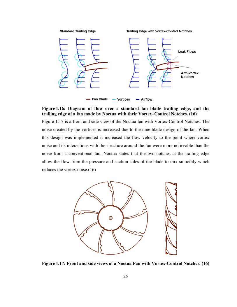
Figure 1.16: Diagram of flow over a standard fan blade trailing edge, and the trailing edge of a fan made by Noctua with their Vortex–Control Notches. (16) Figure 1.17 is a front and side view of the Noctua fan with Vortex-Control Notches. The

noise created by the vortices is increased due to the nine blade design of the fan. When

this design was implemented it increased the flow velocity to the point where vortex

noise and its interactions with the structure around the fan were more noticeable than the

noise from a conventional fan. Noctua states that the two notches at the trailing edge

allow the flow from the pressure and suction sides of the blade to mix smoothly which

reduces the vortex noise.(16)

Figure 1.17: Front and side views of a Noctua Fan with Vortex-Control Notches. (16)

26

1.4 Torque Converter Turbine Noise and Cavitation Noise over Varying Speed Ratio The remainder of this dissertation discusses experimentation done with torque converters

with respect to operation over simulated vehicle take-off. Chapter 2 is a paper discussing

torque converter cavitation desinence during operation. Previous works by Robinette in

(1), (12), and (9) detail torque converter cavitation during stall operation. However, a

torque converter remains in stall only so long as there is not sufficient torque to create

vehicle motion. If cavitation is present at stall, it will cease at some higher speed ratio as

stator torque and turbine torque decrease. If cavitation at stall is at a low level, and

cavitation desinence occurs shortly into the vehicle launch, then noise from cavitation

will not be noticed, and its effect on performance will be of very little consequence. If,

however, torque levels are high enough to sustain cavitation to a high vehicle speed, then

cavitation noise could be objectionable to the vehicle operator and torque converter

performance might be impacted

Chapter 3 describes the methodology used to compare the turbine dynamics in air to the

dynamics in its working fluid, automatic transmission fluid. Since the structure of the

turbine is more highly damped and has more virtual mass when submerged in ATF than

air, the dynamic parameters of the structure might also be different. It was hypothesized

that this might in some way make it possible to determine if a turbine exhibited the

“Turbine Noise” phenomenon discussed in Chapter 4.

The project outlined in the Chapter 4 utilized the previously discussed wireless telemetry

and acoustic methods applied to speed ratio testing to identify and detect a noisy turbine

phenomenon. A 4-6 kHz narrow band noise occurred at mid to high speed ratios in some

converters tested. This noise was eliminated by the addition of trailing edge notches to

the turbine, similar to those described in the Figure 1.17. The “Turbine Noise”

phenomenon was thought to be a result of VonKarman Vortex Shedding coupled with a

natural frequency of the torque converter turbine. The experimentation discussed was

performed to determine if the vortex shedding hypothesis was valid.

27

1.5 References (1) Robinette DL. Detecting and Predicting the onset of Cavitation in Automotive

Torque Converters. PhD Dissertation, Michigan Technological University. Ann Arbor: ProQuest/UMI. 2007.

(2) Arakeri V. Cavitation Inception. Proc. Indian Acad. Sci. 1979; Vol. C2, Pt. 2: pp. 149-177.

(3) Mekkes J, Anderson CL, Narain A. Static Pressure Measurements on the Nose of a Torque Converter Stator during Cavitation. ISROMAC. 2004.

(4) Zeng L, Anderson CL, Sweger PO, Narain A. Experimental Investigation of Cavitation Signatures in an Automotive Torque Converter Using a Microwave Telemetry Technique. ISORMAC. 2002.

(5) Blander M, Katz JL. Bubble Nucleation in Liquids. American Institute of Chemical Engineers. 1975; Vol. 21, No. 5: pp. 833-847.

(6) Reynolds O. On The Dynamical Theory of Incompressible Viscous Fluids and the Determination of the Criterion. Proceedings of the Royal Society of London. 1895.

(7) Strasberg M, Taylor D. Propeller Cavitation Noise after 35 Years of Study. Noise and Fluids Engineering. 1977.

(8) Kowalski D, Anderson CL, Blough JR. Cavitation Detection in Automotive Torque Converters Using Nearfield Acoustical Measurements. SAE-NVH. 5/16/2005; 2005-01-2516.

(9) Robinette DL, Anderson CL, Blough JR, Johnson MA, Maddock DG, Schweitzer JM. Characterizing the Effect of Automotive Torque Converter Design Parameters on the Onset of Cavitation at Stall. SAE-NVH. 5/15/2007; 2007-01-2231.

(10) Alfayez L, Mba D, Dyson G. The Application of Acoustic Emission for Detecting Incipient Cavitation and Best Efficiency Point of a 60 Kw Centrifugal Pump: Case Study. NDT & E International. 2005; Vol. 38, Issue 5: pp. 354-358.

(11) Barna G. IR Telemetrics. 2010.

(12) Robinette DL, Schweitzer JM, Maddock DG, Anderson CL, Blough JR, Johnson MA. Predicting the Onset of Cavitation in Automotive Torque Converters—Part II: A Generalized Model. ISORMAC. 2008; Article ID 312753.

(13) Kowalski D, Anderson CL, Blough JR. Cavitation Prediction in Automotive Torque Converters. SAE-NVH. 2005; 2005-01-2557.

(14) La Rosa Siqueira C. Wikipedia. File:Vortext-street-animation.gif. 2005. http://en.wikipedia.org/wiki/File:Vortex-street-animation.gif.

(15) Blevins R. Flow Induced Vibration. Krieger Publishing Company. 2001

28

(16) Noctua Fan Company. Nine Blade Design with Vortex-Control Notches. 2012; http://www.noctua.at/main.php?show=nine_blade_design&lng=en.

(17) Raabe J. Cavitation Effects in Turbomachinery – European Experiences: Cavitation State of Knowledge. ASME Fluid Engineering Div. 6/1969.

(18) Sweger P, Anderson CL, Blough JR. Measurements of Strain on 310 Mm Converter Turbine Blade. International Journal of Rotating Machinery. 2004; Volume 10, No 1: pp. 55-63.

(19) Wen Y, Henry M. Time Frequency Characteristics of the Vibroacoustic Signal of Hydrodynamic Cavitation. ASME Journal of Vibration and Acoustics. 2002; Vol 124: pp. 469-476.

(20) Arakeri VH, Acosta AJ. Viscous Effects in the Inception of Cavitation on Axisymmetric Bodies. ASME Journal of Fluids Engineering. 12/1973; pp. 519-527.

(21) Baldassarre A, DeLucia M, Nesi P. Real-Time Detection of Cavitation for Hydraulic Turbomachines. Real-Time Imaging. 1998; pp. 403-416.

(22) Blake WK, Wolpert MJ, Geib FE. Cavitation Noise As Influenced By Boundary Layer Development on a Hydrofoil. Journal of Fluid Mechanics. 1977; Vol. 80: pp. 617-640.

(23) Brennen CE. Cavitation and Bubble Dynamics. Oxford University Press. 1995; .

(24) Caron JF, Farhat M, Avellan F. Physical Investigation of the Cavitation Phenomenon. 4th International Symposium on Cavitation. 6/2001.

(25) Chahine GL. Nuclei Effects on Cavitation Inception and Noise. 25th Symposium on Naval Hydrodynamics. 8/2004.

(26) Chen Y, Heister SD. Two-Phase Modeling of Cavitated Flows. Computers and Fluids. 1995; Vol. 24, No. 7: pp. 799-809.

(27) Gu W, He Y, Hu T. Transcritical Patterns of Cavitating Flow and Trends of Acoustic Level. ASME. 2001; Vol. 123: pp. 850-857.

(28) Guennoun F, Farhat M, Bouziad YA, Avellan F. Experimental Investigation of a Particular Traveling Bubble Cavitation. 5th International Symposium on Cavitation. 2003.

(29) Knapp RT, Hammitt JW, Daily FG. Cavitation. Engineering Societies Monographs. 1970.

(30) Kunz R, Boger D, Stinebring D, Checzewski T. A Preconditioned Navier-Stokes Method for Two-Phase Flows with Application to Cavitation Prediction. Computers and Fluids. 2000; Vol. 29: pp. 849-875.

29

(31) Martin CS, Medlarz H, Wiggert DC, Brennen C. Cavitation Inception in Spool Valves. Transaction of ASME. 1981; Vol. 103: pp. 564-576.

(32) McNulty PJ, Pearsall IS. Cavitation Inception in Pumps. ASME Journal of Fluids Engineering. 1982; Vol. 104: pp. 99-104.

(33) Robinette DL, Schweitzer JM, Maddock DG, Anderson CL, Blough JR, Johnson MA. Predicting the Onset of Cavitation in Automotive Torque Converters – Part II: A Generalized Model. International Journal of Rotating Machinery. 2008; Article ID 312753.

31

Chapter 2 – Predicting Cavitation Desinence in Automotive Torque Converters1

C. Walber1, J. Blough2, C. Anderson2, M. Johnson2, J, Schweitzer3

1PCB Piezotronics 3425 Walden Ave Depew, New York, USA email: [email protected] 2 Michigan Technological University, Department of Mechanical Engineering 1400 Townsend Dr. Houghton, Michigan, USA 3 General Motors Powertrain Pontiac, Michigan, USA

2.1 Abstract Cavitation is a concern in automotive torque converters because it can cause operation to

be altered from design intent, generate unaccepTable 2.noise in the passenger

compartment of a vehicle, and damage torque converter components in extreme

situations. Previous cavitation experiments have determined the onset of cavitation in

stall mode. During actual operating conditions, however, torque converter stall occurs for

a short duration. Thus characterization of cavitation in speed ratio operation is needed.

Torque converter speed, torque, and hydraulic parameters at cavitation desinence were

determined experimentally using a dynamometer test cell in concert with nearfield

acoustic measurements. These experimentally determined operating conditions along

with design parameters were used to create a set of dimensionless parameters, which

were used to develop non-dimensional predictive models of the cessation of cavitation

during simulated vehicle takeoff. Models were developed for several groups of torque

converters with varying degrees of similitude.

1 The material contained in this chapter has been submitted to the International Journal of Rotating Machinery.

mailto:[email protected]

32

2.2 Introduction The automotive torque converter is the powertrain component that multiplies engine

torque to overcome the poor low speed torque characteristics of an internal combustion

engine. It regulates engine speed to evenly increase during vehicle acceleration. Modern

automotive torque converters are made up of three elements, a mixed flow pump and

turbine, and an axial flow stator. Figure 2.1 is a basic schematic of a torque converter,

including arrows showing the direction of the toroidal flow induced during operation.

Maximum efficiency is achieved during high speed ratio operation while maximum

torque multiplication is attained at stall, or turbine speed equal to zero. Speed ratio (SR)

is defined as the ratio of the turbine speed over the pump speed.

In the basic operation of a torque converter, the pump is driven by the engine through


Rotation of the pump imparts angular momentum onto the automatic transmission fluid

(ATF). The fluid flows from the inner radius of the pump flow path to the outer radius,

and is directed into the turbine. The angular momentum of the fluid acts on the turbine,

imparting a torque to the turbine shaft which is the input shaft to the automatic

transmission. The fluid exits the turbine and is redirected by the stator toward the pump at

a favorable angle with regards to pump operation. The change in angular momentum by

the stator is what creates torque multiplication. The torque multiplication factor, called

torque ratio (TR), is the performance characteristic that helps the vehicle accelerate from

a stop.

33

Figure 2.1: Cross section of an automotive torque converter; toroidal flow is indicated by the direction of the arrows with no tail. Arrows with tails indicate the normal cooling flow (1) Maximum torque multiplication occurs at stall. As turbine speed and speed ratio increase,

torque ratio decreases. This is due in part to the change in flow incidence angle into the

stator. The angle of flow exiting the turbine relative to the stator blade inlet angle

decreases with increasing turbine speed such that the change in angular momentum

across the stator decreases, and stator torque decreases. At a high speed ratio, the

incidence angle lines up with the stator blade inlet angle, and torque multiplication

becomes one. Up to this point of operation, the stator is grounded to the stator shaft and

does not rotate. As turbine speed further increases, incidence angle rotates around the

nose of the stator blade such that flow impacts the stator blades on the opposite side. To

prevent torque ratio from becoming less than one, the stator assembly has a one-way

clutch that allows it to overrun, effectively getting out of the way of the flow. At the point

when the stator overruns, the converter is acting as a fluid coupling. The speed ratio at

which the stator overruns is called the coupling speed ratio. Progression of incidence

angle with speed ratio is depicted in Figure 2.2.

34

Torque converters need temperature control to prevent overheating of the ATF. Under

practical operation, a converter functions at less than unit efficiency, and all power loss is

converted to heat within the working fluid. The automatic transmission pump forces a

continuous flow of cooling fluid through the torque converter. ATF flows into the

converter between the cover and the clutch, and then into the outer torus region between

the pump and the turbine where it is integrated into the toroidal flow. The direction of

this flow is indicated in Figure 2.1 by the maroon arrows. The hotter fluid is evacuated

from the converter to the vehicle cooling system. A second function of the transmission

pump is to control the level of pressure in the torque converter to suppress cavitation. The

flow into the converter is called charge pressure, and the flow out is called back pressure.

Figure 2.2: Flow incidence angle across the blades of the stator (1) When the torque converter is operating at high speed ratios, a clutch can be engaged to


hydrodynamic inefficiency of the torque converter. The clutch is engaged by reversing

this cooling flow, pushing the pressure plate of the clutch toward the cover of the

converter. Apply pressure is regulated to create a full lock between the cover and clutch,

or a controlled speed slip.

In torque converter mode, individual element torques are created from the change in

angular momentum flux across an element from inlet to outlet. The torque is a function of

the local static pressure times the radius integrated over the entire surface of each blade.

Low Pressure Side

High Pressure Side

35

A greater pressure differential across a blade proportionally increases the individual

element torque. Consequently, at some large element torque, the pressure on the low

pressure side of a blade can drop to below the vapor pressure of the fluid, and the

nucleation of cavitation bubbles may occur.

The effect of cavitation on performance is dependent on whether sustained cavitation is

reached. Incipient cavitation can occur at stall and dissipate before it is of any

consequence. But if a high level of element torque is sustained for a long duration, the

heavy cavitation will result in large vapor regions that displace the working fluid, affect

performance, and possibly cause damage when cavitation bubbles collapse. Furthermore,

collapsing bubbles cause a broadband noise that may affect the overall sound quality of

the vehicle. Advanced cavitation causes a decrease in individual element torques, which

alters the relationship between speed and torque for the converter.

2.3 General Considerations Torque Converter Cavitation at Stall - In previous research, Robinette et al. (1) and

Kowalski et al. (2) studied torque converter cavitation in depth with the converter

operating at stall. This is the condition at which a torque converter is most susceptible to

cavitation due in part to the high element torques. Toroidal flow within a converter is

highly three dimensional with large element flow incidence angles. The high angle of

flow into the stator at stall creates regions of separated flow on the low pressure side of

the blade. Research by Mekkes et al. (3) confirmed that cavitation initiates in the

separated flow region at the stator inlet. As speed ratio increases, stator torque decreases,

and flow incidence angle becomes less severe. Regions of separated flow are reduced,

and the pressure differential across a stator blade drops, reducing the likelihood of

cavitation bubbles forming at the inlet of the stator.

Mekkes (3) used wireless microwave telemetry to measure pressure at the stator inlet.

The telemetry was placed on the stator, and pressure measurements were made at the

inlet region of the blades. Wireless telemetry was required due to the difficulty in running

wires from inside a rotating torque converter to the data acquisition equipment. The

telemetry was used to acquire pressure measurements from taps on stator blades and to

36

transmit readings to an antenna through the pump via a series of RTV filled slits milled

out of the pump/stator interface. This antenna carried the signal to a receiver which

converted it back to the raw data for a data acquisition system. A method was developed

by Kowalski (2) that uses nearfield acoustic measurements to accurately detect cavitation

without requiring wireless telemetry. In this way, a large population of torque converters

can be tested for cavitation without the time and expense needed to create microwave

instrumented torque converters for each blade design of interest. Robinette et al. (4) used

the acoustic method to determine incipient cavitation at stall for a population of torque

converters with a wide range of sizes and blade geometries. A correlation was formulated

based on operating conditions and converter geometry to estimate the point of incipient

cavitation during stall.

Speed Ratio Operation - A torque converter remains in stall only so long as there is not

sufficient torque to create vehicle motion. If cavitation is present at stall, it will cease at

some higher speed ratio as stator torque and turbine torque decrease. If cavitation at stall

is at a low level, and cavitation desinence occurs shortly into the vehicle launch, then

noise from cavitation will not be noticed, and its effect on performance will be of no

consequence. If, however, torque levels are high enough to sustain cavitation to a high

vehicle speed, then cavitation noise could be objectionable to the vehicle operator.

Therefore, it is important to characterize the duration of cavitation versus speed ratio with

respect to torque converter design parameters and operating conditions. This project

utilized the previously developed acoustic method that was used to identify incipient

cavitation, but applied it to speed ratio testing to identify cavitation desinence.

2.4 Experiment A dynamometer test fixture was constructed for taking acoustic data with torque

converters during the previous stall cavitation project. The fixture is much larger than

typically used for torque converter testing so that it can be filled with acoustic foam to

assist in absorbing and insulating noise. Figure 2.3 shows pictures of both a typical torque

converter test fixture and the acoustically treated fixture used for the cavitation

37

experiments. On the right is a picture of the fixture opened to reveal a torque converter

and acoustic foam.

Figure 2.3: Left: Comparison of original torque converter dynamometer test fixture (red) and acoustic test fixture (gray). Right: Close up of opened acoustic test stand with acoustic foam (1) The SR test procedure was developed to emulate torque converter performance during

vehicle takeoff with the engine running at constant torque. During a test, the turbine

speed is accelerated at a steady rate while the pump is held at a fixed torque. The first

step in the test procedure is to bring the pump up to the torque it will sustain throughout

the experiment. A short settling period is needed to allow speed transients due to the

control system to settle out. The turbine is then ramped at 50 rpm/s from low speed (100

rpm) to high speed (2500 rpm). An upper speed of 2500 rpm was selected to achieve high

enough speed ratio to ensure that cavitation desinence would occur for any of the torque

converters planned to be tested. After the test is completed, a torque correction factor

which includes dynamic torque losses due to the entire dynamometer system is applied to

the measured torques. As with all torque converter testing, speeds, torques, pressures,

temperatures, and flow rates are collected via the control system at a 10 Hz sample rate.

Nearfield acoustic measurements are taken at a 51.2 kHz sample rate. Pump and turbine

speeds then are also measured at 51.2 kHz so that some reference may be made between

the acoustic data and other test parameters.

Speed ratio sweeps were conducted for each torque converter at various input torques and

charge pressures. Charge pressures tested were 480, 690, 900, 1030, and 1240 kPa with a

38

pressure delta of -210 kPa for the back pressure. Cooling flow temperature was held

constant throughout all of the tests at 70°C. Input torque for each test was selected based

on the torque required to initiate cavitation stall in the previous stall testing plus 70 Nm.

The extra torque was added to make sure that cavitation occurred during the speed ratio

test. The minimum input torque used was 150 Nm and the maximum was 310 Nm for the

torque converters in this study.

Figure 2.4: Example of torque converter speed ratio data plot

The goal of the speed ratio testing was to determine the desinence of cavitation, or the

point at which the bubbles can no longer be detected within the working fluid. In the stall

testing by Robinette (1), incipient cavitation was characterized by a sudden increase in

the amplitude of the high pass filtered sound pressure level (SPL) of the noise

measurements. This SPL was further processed into a slope2 curve, which was then used

as an indicator function to determine the onset of cavitation. A similar approach is taken

to determine cavitation desinence. Figure 2.4 is a colormap from a SR test showing the

nearfield noise versus SR and frequency. Overlaid on the plot are the filtered SPL curve

and the slope2 curve of SPL normalized to the sound pressure level so that both curves

can be plotted on the same graph. The slope2 curve is used to facilitate identifying the

key changes in the SPL curve. The region of high broadband noise on the left half side of

the colormap corresponds to cavitation. The high magnitude peak in the slope2 curve

near 0.4 SR corresponds to the desinence of cavitation.

39

2.5 Analysis Preliminary Data - After data for a torque converter SR test is acquired, the speed ratio

at desinence of cavitation, labeled SRd, needs to be identified. During speed ratio

operation, however, the noise from the turbine and pump increases as turbine speed

increases, and the overall noise content of the converter is complex. This is evidenced by

the numerous local peaks and valleys in the SPL curve in Figure 2.4. SPL drops to a

fairly constant level after cavitation stops, but the roughness of the curve and the lack of a

sharp transition from the cavitation region to non cavitation necessitated the development

of a repeaTable 2.and objective procedure for identifying SRd. Figure 2.5 demonstrates

the method that was used.

Figure 2.5: Visualization of the algorithm used to determine desinent cavitation in a torque converter The top portion of Figure 2.5 shows the filtered SPL curve. A high pass filter with a

cutoff of 10 kHz is used to filter out the background noise, rotational orders, and blade

pass frequencies that occur below 10 kHz. The resulting filtered SPL curve displays the

wideband noise from cavitation. As expected, cavitation noise is highest near stall, and

gradually decreases to a relatively constant level when cavitation bubbles cease to form.

A lower high pass filter of 6 kHz was used in the analysis by Robinette (1) due to less

40

background noise being present in stall testing. Due to the jagged nature of the SPL

curve, it is smoothed using a three point running average filter. This curve is then used to

generate a slope2 curve plotted as a percentage as shown in the bottom portion of Figure

2.5. The resulting curve is examined to find the maximum speed ratio less than 0.65

where the slope2 curve is greater than 22.5 percent of its maximum. The 0.65 SR limit

was determined after examining data from all the tests and finding that cavitation always

ends at a lower speed ratio. The 22.5 percent slope2 threshold was selected after

studying the data from all the tested converters and selecting a level that correlated with

the perceived change in the SPL over the entire population. These criteria were entered

into an algorithm to search for the points of cavitation desinence from all the test runs.

Figure 2.5 shows the resulting slope2 curve from the colormap in Figure 2.4 with the

excluded areas shaded out in the lower plot, and the determined point of desinent on both

plots. The fluid parameters required for further analysis are taken at the speed ratio of

cavitation desinence.

Dimensional Analysis - Dimensional analysis was used to develop models for predicting

torque converter cavitation desinence using torque converter design parameters and

operating parameters measured or controlled in the speed ratio tests. In the stall cavitation

research done by Robinette (4), a set of dimensionless parameters that incorporates

torque converter design variables, performance parameters and operating conditions was

derived and used to develop dimensionless models to predict the emergence of cavitation

at stall. Similar parameters were used in this study to develop models for cavitation

desinence, but were modified somewhat to accommodate speed ratio operation. These are

listed in Table 2.1.

41

Table 2.1: Dimensionless Parameters used in Speed Ratio Correlation

Unit Input

Speed

Based on overall torque

converter design

Stall Torque

Ratio

Based on overall torque

converter design

Torus Aspect

Ratio

Based on torque converter

geometry

Stator Blade

Thickness

Ratio


geometry

Number of

Stator Blades


geometry

Dimensionless

Pressure Ratio Operating Point Parameter

Prandtl

Number Operating Point Parameter

Dimensionless

Rotational

Power

Combination of Operating

Point Parameter and Measured

Response

Unit input speed at stall, U, shown in Equation 1, is a parameter that describes torque

converter performance and is used to select the best torque converter for a given engine

and vehicle application. It contains the relationship between the working fluid (density),

the size of the converter (diameter), the input speed, and the input torque.

(1)

The value of U is a function of the blade designs for the pump, turbine, and stator. It is

used in the dimensional analysis instead of using a longer list of blade design parameters.

42

Torque Ratio was described earlier as the ratio of output torque over input torque. Note

that since both U and TR have a dependence on speed ratio, the values of these variables

at stall were used for this correlation to improve equation conditioning.

Torus aspect ratio is a definition of the roundness of a torque converter. The

measurements used for this along with stator blade thickness ratio are shown in Figure

2.6. The number of stator blades is a design variable that is a function of stator blade

angles and the axial length of the stator.

Figure 2.6: Left: Schematic of torque converter showing diameter (D) and torus length (Lt) Right: Profile of stator blade depicting maximum thickness (tmax) and chord length (lc) (1) The dimensionless pressure ratio and the Prandtl number are calculated from the values

of the measured charge and back pressures, flows, and temperature taken due to the

cooling flow mentioned in the introduction. The formulations of these parameters are

shown in Equations 2 and 3. In Equation 2, pcharge and pback are the charge and back

pressures applied to the test stand during operation respectively. The term, cp, in

Equation 3, is the specific heat of the working fluid, k is the thermal conductivity, and µ

is the dynamic viscosity. All of these values are measured or calculated based on the

temperature at the point of cavitation desinence.

(2)

(3)

43

The last dimensionless group, Dimensionless Rotational Power, is the product of the

speed ratio at desinent cavitation, SRd, (selected by the algorithm detailed in Section 3)

and the dimensionless input torque. This combination of dimensionless parameters was

selected as the dimensionless response in the correlation development because it is

defined by quantities that can be used to assess the potential for cavitation in a new

torque converter design or a new application of an existing design.

The dimensionless groups are applied to a Response Surface Model (RS) using a

stepwise regression procedure to predict the dimensionless rotational power. The general

form of the response surface model is outlined in the research of Madsen et al. (6), and is

given here by Equation 4.

(4)

The response, ŷ, is dimensionless rotational power, while the linear, quadratic, and

interaction terms are generated from the other dimensionless regressors listed in Table

2.1. These are used to solve for the β0, βii, and βij terms using a least squares method.

The residual error, symbolized in Equation 4 as ε, is the difference between the

experimentally measured quantity of the dimensionless rotational power and the

predicted value.

A forward selection path of stepwise regression is used to minimize the error in the

models. This method starts with a basic equation comprised of only the intercept term,

β0. From there, regressors are added until the error of the model is minimized. At each

step the response is calculated using all of the remaining regressors in addition to those

that had previously been added, after which the new regressor is selected by determining

which one minimizes the error to the greatest degree.

The quality of fit for any RS model is verified by the root mean square error (RMSE) and

by determining the linear association between the dimensionless response and the

regressors. RMSE estimates the model’s standard deviation and for these correlations are

computed as a percentage. Equation 5 shows the calculation for %RMSE. The term yi is

44

the dimensionless rotational power, ŷi is the calculated response from the model, n is the

number of data points, and p is the number of dimensionless regressors in the model.

(5)

The proportionate amount of variation in the response explained by a particular set of

regressors in the model is measured using the adjusted coefficient of multiple

determination, R2a, in Equation 6. This metric calculates to between 0 and 1. Generally,

results above .85 signify an accurate model of the data in question. The coefficient of

multiple determination, R2, was also calculated. However, it is not preferred as the value

of R2 always increases with the addition of regressors. R2a may increase or decrease

depending on whether or not the additional terms actually reduce variation in the

response.

(6)

Figure 2.7 shows results from the stepwise regression procedure for the analysis of a

population of round torus torque converters to determine the regressors to be added to the

model. Each step of the procedure optimizes the %RMSE, the R2a, or both. Only those

regressors that have a significant impact on model error or linear association between the

response and the regressors are included in the model. This makes the final model for the

example population a function of 16 terms, including the intercept term, instead of the 36

possible terms. The value for R2a was brought to above .85 within the first three

iterations. Each subsequent iteration was done to improve model error.

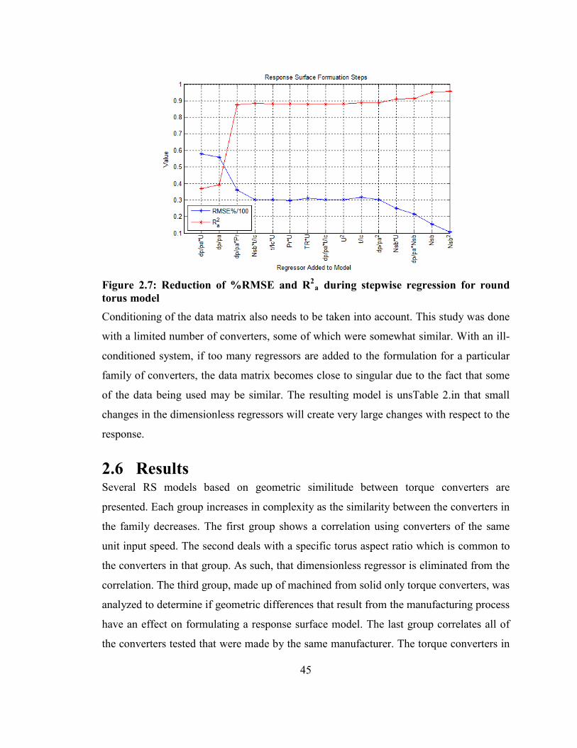
45

Figure 2.7: Reduction of %RMSE and R2

a during stepwise regression for round torus model Conditioning of the data matrix also needs to be taken into account. This study was done

with a limited number of converters, some of which were somewhat similar. With an ill-

conditioned system, if too many regressors are added to the formulation for a particular

family of converters, the data matrix becomes close to singular due to the fact that some

of the data being used may be similar. The resulting model is unsTable 2.in that small

changes in the dimensionless regressors will create very large changes with respect to the

response.

2.6 Results Several RS models based on geometric similitude between torque converters are

presented. Each group increases in complexity as the similarity between the converters in

the family decreases. The first group shows a correlation using converters of the same

unit input speed. The second deals with a specific torus aspect ratio which is common to

the converters in that group. As such, that dimensionless regressor is eliminated from the

correlation. The third group, made up of machined from solid only torque converters, was

analyzed to determine if geometric differences that result from the manufacturing process

have an effect on formulating a response surface model. The last group correlates all of

the converters tested that were made by the same manufacturer. The torque converters in

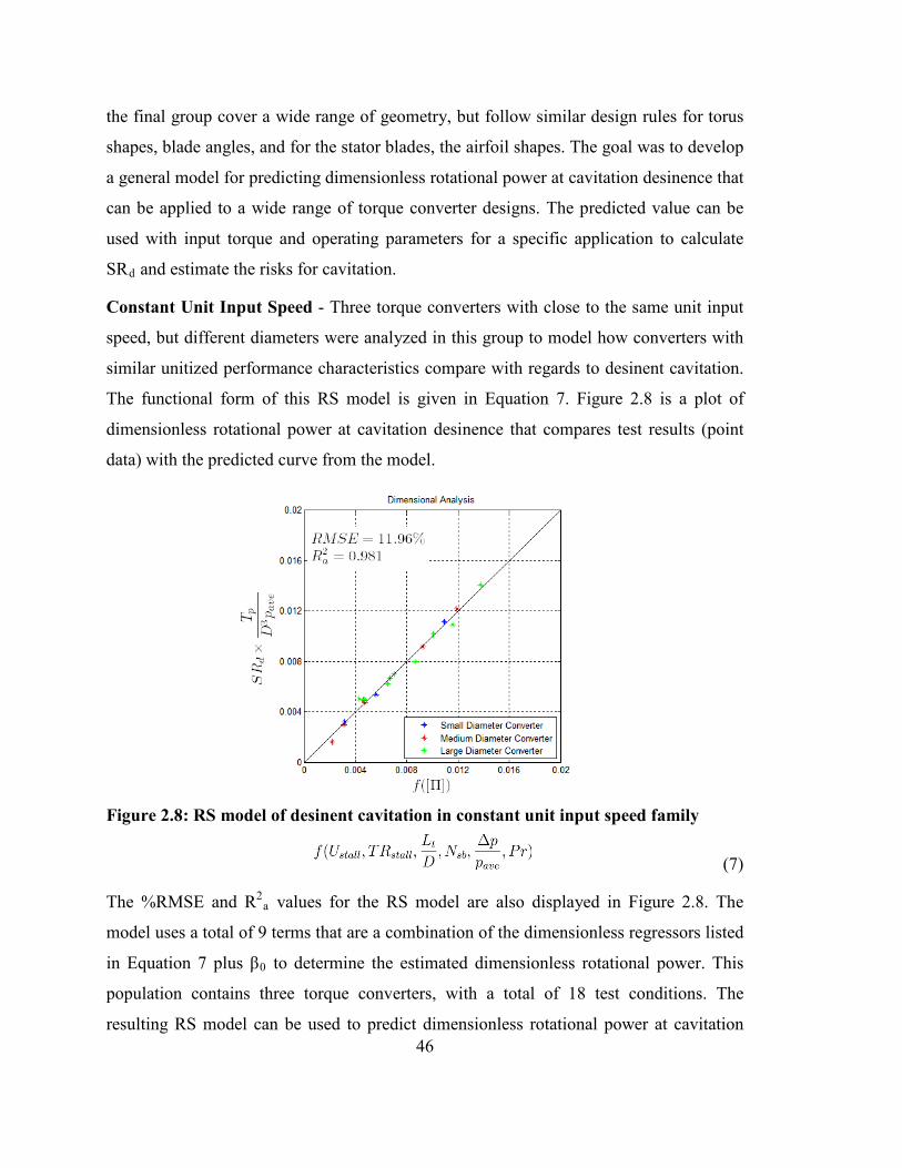
46

the final group cover a wide range of geometry, but follow similar design rules for torus

shapes, blade angles, and for the stator blades, the airfoil shapes. The goal was to develop

a general model for predicting dimensionless rotational power at cavitation desinence that

can be applied to a wide range of torque converter designs. The predicted value can be

used with input torque and operating parameters for a specific application to calculate

SRd and estimate the risks for cavitation.

Constant Unit Input Speed - Three torque converters with close to the same unit input

speed, but different diameters were analyzed in this group to model how converters with

similar unitized performance characteristics compare with regards to desinent cavitation.

The functional form of this RS model is given in Equation 7. Figure 2.8 is a plot of

dimensionless rotational power at cavitation desinence that compares test results (point

data) with the predicted curve from the model.

Figure 2.8: RS model of desinent cavitation in constant unit input speed family

(7)

The %RMSE and R2a values for the RS model are also displayed in Figure 2.8. The

model uses a total of 9 terms that are a combination of the dimensionless regressors listed

in Equation 7 plus β0 to determine the estimated dimensionless rotational power. This

population contains three torque converters, with a total of 18 test conditions. The

resulting RS model can be used to predict dimensionless rotational power at cavitation

47

desinence with less than 12 %RMSE for torque converter designs with this unit input

speed. It should be noted that although the values for unit input speed for the three

converters in this population are very close, they are not identical.

Round Torus - The next family contains torque converters with a large torus aspect

ratio, considered to be round in shape. As similarity of torus ratio exists between all of

these converters, that regressor was ignored in computing the correlation. This population

contains six torque converters with a total of 49 test conditions. The converters are

comprised of a range of component blade designs. Due to greater design diversity as

compared to the constant unit input speed population, more terms, a total of 16, are

required to minimize the model error. Figure 2.9 shows the model diagnostics, as well as

the plot of measured response versus response calculated from regressors. Equation 8 is

the functional form of the RS model. The model from this group can be used to predict

dimensionless rotational power for torque converters with similar torus aspect ratio as

this population with less than 11 percent error.

Figure 2.9: RS model of desinent cavitation in torque converters with a round torus shape

(8)

Similar to the case with the unit input speed population, there was some small variation in

the torus aspect ratio with this group. However, because that regressor did not appear

48

dominant when making this formulation, it was omitted from the final response

calculation.

Machined From Solid Torque Converters - The population of the RS model shown in

Figure 2.10 is made up of torque converters with machined from solid (MFS) pump,

turbine, and stator assemblies. The MFS components are one off prototypes with tight

size tolerances and sealed flow passages. Production pumps and turbines are made from

stamped sheet metal blades and housings, and can have small leak paths between blades.

MFS stator blades surfaces have a smoother surface finish than blades from a typical

production cast stator.

The population for this model contained six torque converters and 46 test conditions. A

total of 17 terms, comprised of all the possible dimensionless regressors and β0, were

used to calculate the response in this model. The torque converters in this group were

made up of a range of diameters, torus aspect ratios, and blade designs such that all of the

dimensionless regressors are significant to the model. Equation 9 shows the functional

from of the response surface model.

Figure 2.10: RS model of desinent cavitation in machined from solid torque converters

(9)

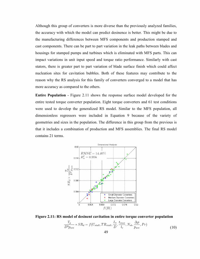
49

Although this group of converters is more diverse than the previously analyzed families,

the accuracy with which the model can predict desinence is better. This might be due to

the manufacturing differences between MFS components and production stamped and

cast components. There can be part to part variation in the leak paths between blades and

housings for stamped pumps and turbines which is eliminated with MFS parts. This can

impact variations in unit input speed and torque ratio performance. Similarly with cast

stators, there is greater part to part variation of blade surface finish which could affect

nucleation sites for cavitation bubbles. Both of these features may contribute to the

reason why the RS analysis for this family of converters converged to a model that has

more accuracy as compared to the others.

Entire Population - Figure 2.11 shows the response surface model developed for the

entire tested torque converter population. Eight torque converters and 61 test conditions

were used to develop the generalized RS model. Similar to the MFS population, all

dimensionless regressors were included in Equation 9 because of the variety of

geometries and sizes in the population. The difference in this group from the previous is

that it includes a combination of production and MFS assemblies. The final RS model

contains 21 terms.

Figure 2.11: RS model of desinent cavitation in entire torque converter population

(10)

50

The RS model for this group essentially creates a generalized model to calculate the point

of desinent cavitation of a converter during speed ratio operation. Equation 10 shows the

functional form of the correlation for the entire converter population tested. The RS

model can be used to predict dimensionless rotational power at desinent cavitation with

14.4 %RMSE for torque converters that follow similar design rules for torus shapes and

blade designs as those that were tested.

Model Discussion - A summary of the RS model equations for all four groups minus

regression coefficients is listed in Table 2.2. The number of regression terms required to

achieve desired accuracy increases with wider ranges of geometric design and

performance parameters due to more interaction between parameters. All of the RS

model equations include contributions from operating parameter and design parameter

regressors.

51

Table 2.2: RS Models by Torque Converter Population minus Regression Coefficients

Population Response surface model

Constant Unit Input

Speed

Round Torus

Machined from Solid

Entire Population

In contrast to the models developed by Robinette (4) to predict incipient cavitation at

stall, the models for cavitation desinence have larger values for %RMSE. One contributor

could be that the torque converters in the stall cavitation study were all comprised of

MFS components. The RS model for the MFS population in this study has the highest

accuracy of any of the groups. Greater model accuracy could be from less variation in

SRd for a family of MFS converters due to reduction in part to part variation in blade

52

surface finish for MFS stators as compared to die cast and to the elimination of small

blade to housing flow paths in MFS pumps and turbines.

The turbine speed sweep rate might also be a factor in model accuracy. While the turbine

acceleration that was used in dynamometer testing is not as fast as in a typical vehicle at

wide open throttle, a slower sweep rate might reduce errors from the transient response of

the torque converter dynamometer. Additional speed ratio testing at different rates could

be done to measure potential influence.

2.7 Conclusions A method was developed to determine the speed ratio of cavitation desinence in

automotive torque converters by testing on a dynamometer and using acoustic

measurements. Desinent cavitation for torque converters of various geometries was

determined, and corresponding data was used to formulate RS models by which it can be

predicted. The torque converter geometries and operating parameters of the working fluid

were used as dimensionless regressors, while dimensionless rotational power was used as

the dimensionless response. A stepwise regression analysis was used to simplify each

model so that only the regressors that significantly reduced the error in the model while

enhancing the model’s predictive capability were included.

Test results from several populations of torque converters were analyzed to create RS

models. As populations increase in diversity, the models are more complex. The RS

models that were created based on the converters having similar geometric properties

(Torus aspect ratio) or similar operating capacities (Unit input speed) are capable of

predicting the dimensionless rotational power of the converter at the point of desinent

cavitation within a %RMSE of 10.8 and 11.6 percent respectively. The general model

developed from test results for all the converters tested is capable of predicting

dimensionless rotational power at desinent cavitation with 14.4 %RMSE. The R2a of all

models presented is greater than .85, making each of them useful as an accurate model to

estimate the dimensionless rotational power.

53

2.8 References (1) Robinette DL. Detecting and Predicting the onset of Cavitation in Automotive Torque

Converters. PhD Dissertation, Michigan Technological University. Ann Arbor: ProQuest/UMI. 2007.

(2) Kowalski D, Anderson CL, Blough JR. Cavitation Detection in Automotive Torque Converters Using Nearfield Acoustical Measurements. SAE-NVH. 5/16/2005; 2005-01-2516.

(3) Mekkes J, Anderson CL, Narain A. Static Pressure Measurements on the Nose of a Torque Converter Stator during Cavitation. ISROMAC. 2004.


(5) Dong Y, Lakshminarayana B. Rotating Probe Measurements of the Pump Passage Flow Field in an Automotive Torque Converter. ASME J. of Fluids Eng.. 2001; Volume 123: pp. 81-91.

(6) Madsen JI, Shyy W, Haftka RT. Response Surface Techniques for Diffuser Shape Optimization. AIAA Journal. 2000; Volume 38, No 9: pp. 1512-1518.

(7) Strasberg M, Taylor D. Propeller Cavitation Noise after 35 Years of Study. Noise and Fluids Engineering. 1977.


55

Chapter 3 – Measuring and Comparing Frequency Response Functions of Torque Converter Turbines Submerged in Transmission Fluid1

C. Walber, J. Blough, C. Anderson, M. Johnson

Michigan Technological University, Department of Mechanical Engineering

1400 Townsend Dr. Houghton, Michigan, USA Copyright © 2011 SAE International

3.1 Abstract When testing dynamic structures, it is important to note that the dynamic system in

question may be submerged into a fluid during operation and to properly test the structure

under the same condition in order to understand the true dynamic parameters of the

system. In this way, the mass and stiffness coupling to the particular fluid, for the case of

this study, automatic transmission fluid, may be taken into account. This is especially

important in light structures where the coupling between the fluid mass and the structural

mass may be great. A structure was tested with a laser vibrometer using several impact

methods in open air to determine which impact method would be most suiTable 3.for

submerged testing. The structure was then submerged in transmission fluid with an

accelerometer attached and subsequently tested and compared to the previous results. In

addition, two novel means of excitation, by use of a ball bearing impact and by use of a

weighted impact rod, will also be discussed and compared.

1 The material contained in this chapter has been published in the Journal of SAE Noise and Vibration

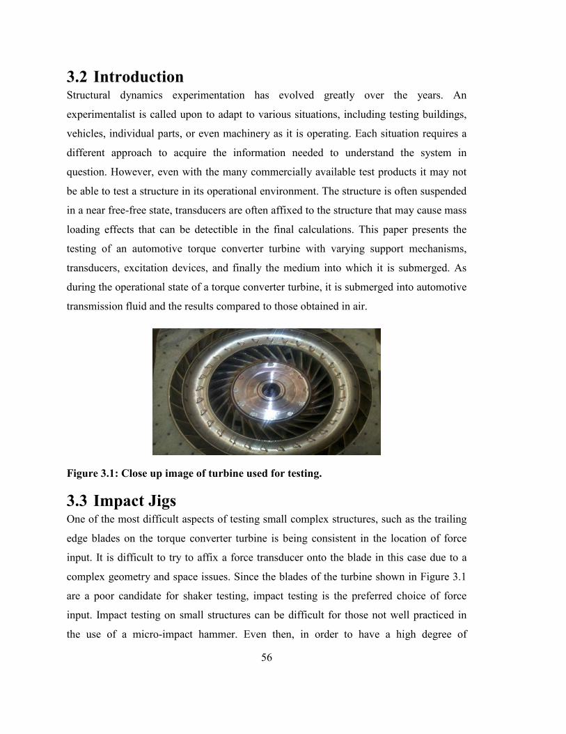
56

3.2 Introduction Structural dynamics experimentation has evolved greatly over the years. An

experimentalist is called upon to adapt to various situations, including testing buildings,

vehicles, individual parts, or even machinery as it is operating. Each situation requires a

different approach to acquire the information needed to understand the system in

question. However, even with the many commercially available test products it may not

be able to test a structure in its operational environment. The structure is often suspended

in a near free-free state, transducers are often affixed to the structure that may cause mass

loading effects that can be detectible in the final calculations. This paper presents the

testing of an automotive torque converter turbine with varying support mechanisms,

transducers, excitation devices, and finally the medium into which it is submerged. As

during the operational state of a torque converter turbine, it is submerged into automotive

transmission fluid and the results compared to those obtained in air.

Figure 3.1: Close up image of turbine used for testing.

3.3 Impact Jigs One of the most difficult aspects of testing small complex structures, such as the trailing

edge blades on the torque converter turbine is being consistent in the location of force

input. It is difficult to try to affix a force transducer onto the blade in this case due to a

complex geometry and space issues. Since the blades of the turbine shown in Figure 3.1

are a poor candidate for shaker testing, impact testing is the preferred choice of force

input. Impact testing on small structures can be difficult for those not well practiced in

the use of a micro-impact hammer. Even then, in order to have a high degree of

57

repeatability while performing impact testing, it is wise to create a jig to assist in both

automating the impacts and making their amplitudes and position more repeatable.

The first jig discussed here is a very simple concept whereby a known, yet unmeasured,

force created by a ball bearing impacting the structure is used as the excitation. This is a

very precise method of maintaining consistency in the amplitude of the input force as

well as the location of the impact. The second jig is an evolution of the first, replacing the

ball bearing with a weighted rod, onto which a force transducer is affixed, thereby

collecting an actual measurement of the input.

3.4 Ball Bearing Impact The first jig takes advantage of Newton’s Second Law to calculate the force input into the

structure in lieu of a force transducer. The excitation is applied by means of using ball

bearings of a known mass, and dropping them down a guide tube onto the blade so that

they impact the same point on the structure with each drop. This method has shown to

have a high degree of repeatability. The amount of energy to be put into the structure can

be adjusted via the mass of the ball bearings or the height from which they are dropped.

Equation 1 is Newton’s Law modified for dropping the ball bearings onto any structure.

The mass of the ball bearing is mbb, g is the acceleration due to gravity, and θvert is the

angle the surface of the structure makes with vertical.

Fimpact=mbb*g*sin(θvert) (1)

This equation gives a force which is used to create an artificial impact time history using

a unit impulse function. The impulse is multiplied by the magnitude of the force and the

autopower calculated. This autopower spectrum, seen in Figure 3.5 below, is then used to

normalize each average of the autopower of the response, which in this case was

measured by a laser vibrometer.

The ball bearing jig itself, shown in Figure 3.2, is simply a fixed tube aimed at the

structure through which a ball bearing is dropped. Rough aiming is done by sighting the

point of impact on the structure through the guide tube, small changes can be made

58

afterward by several test drops to check positioning. It is very important that this jig is

very sturdy so that the point of impact does not vary. Also the tube to be used should be

very smooth on the inside, as a rough surface will make the ball bearing path more

erratic. It is also required that the path of the ball bearing allows for it to impact the

structure only once as with this method it is more difficult to determine whether a double

hit occurred with the lack of a measured time history or autopower of the excitation.

When using this jig in concert with a laser vibrometer, it must also be set up to make sure

that the ball bearing does not cross the beam and interrupt the measurement. Alternately,

when using this jig with accelerometers, it is inadvisable to impact the accelerometer

directly, as this is not a true means of exciting the structure, and may cause the transducer

to overload due to the direct impact.

Figure 3.2: Image of the ball bearing drop jig. The red dot is the laser vibrometer reflecting off of the trailing edge blade of the turbine. The guide tube comes down from the upper right portion of the picture to guide the ball bearing to impact near the laser dot.

The ball bearing method isn’t a perfect means by which to excite a structure, but it is a

very good means by which to have a high degree of repeatability with your excitation on

very small structures. The greatest drawback to this method is that the excitation point on

the structure must allow for the ball bearing to drop away from the structure so that it

does not create a double hit. As a result, it is almost impossible to use an input point that

is on the top of a structure. Also, when using this method, it is impossible to collect true

phase data. The exact moment at which the ball impacts the structure is unknown, and

59

cannot be used as a phase reference. This also gives somewhat of an uncertain result with

regards to the magnitude of the input as it is based on an idealized model. This effect is

seen in Figure 3.4 when compared with the next method of excitation, in which the input

force is measured instead of estimated.

3.5 Impact Rod A second excitation method that was developed for this structure is an impact rod. This

jig evolved from the previous in the use of a guide tube to accurately direct the input

force. Not quite as compact or simple as the ball bearing method described above, this

method has the advantage of being able to use an actual force transducer to measure the

force imparted on the structure. This assembly also allows for very good repeatability in

reference to the point of impact. Any discrepancy with regards to the energy input to the

structure is alleviated because the input force is directly measured by the force

transducer.

A stinger with a weight threaded on one end was slid first through a spring from a

retracTable 3.ball point pen and then a steel tube. The end opposite the spring on the

stinger is outfitted with a two part chuck assembly. An impact cap is threaded into the

base of the chuck to create a smooth surface for the head from a micro-impact hammer to

be glued securely. The entire striker assembly is shown in Figure 3.3. The guide tube of

this assembly is clamped into a fixture similar to the tube into which the ball bearing

assembly was clamped.

Figure 3.3: Photo of impact rod assembly depicting the various parts used.

60

After an impact, the spring draws the rod assembly back to prevent it from impacting

again. Double-hits are avoided easily by adjusting the initial distance of the tip from the

impact point on the structure. As with the ball bearing method, the support structure

should be very sturdy to prevent a loss of alignment over the various impacts. One of the

main advantages of this method over the ball bearing method is that the rebound is

controlled by the spring, not gravity. This means that the impact rod can be used on the

structure at various angles and even on the top of the structure without worry of a second

impact. The greatest disadvantage of this jig is the required clearance required to set it up.

The length of the rod can be shortened, however it still will not allow it to be used in very

cramped spaces.

3.6 Comparison of Input Methods Figure 3.4 shows how the response of the structure is slightly different depending on the

excitation method used. The FRFs from both methods in general agree quite well. The

frequencies all line up, and even the amplitude at higher frequencies is very close. The

difference in amplitude at the lower frequencies could be attributed to the fact that the

impulse used to characterize the impact of the ball bearing was an ideal impulse, which is

the amplitude of the force of the ball bearing on a perfectly rigid structure at one sample

point in a time history. This would translate in the FFT as a perfectly flat response across

all frequencies. An actual impact on the structure varies from this ideal model.

Figure 3.5 shows the comparison of the normalized autopower spectra between the

impact methods. The time histories of both input methods were normalized by their

maximum values as the amount of force in each impact were different. The larger

amplitude in the measured autopower at lower frequencies explains how the FRF

response for that input method might be smaller at those frequencies.

From these plots it can be stated that both methods are successful at exciting the structure

to measure an FRF. In the event that a transducer to properly measure the input is

unavailable, or that the structure in question is very difficult to impact with a high degree

of repeatability due to small size, it is possible to collect FRF measurements using the

61

ball bearing method. As stated earlier, this method sacrifices the phase data, and must be

setup properly in order to maintain accuracy of input location.

Figure 3.4: Plot comparing FRFs taken using a ball bearing as the excitation and the impact rod.

Figure 3.5: Plot comparing the autopower spectra of the "Ideal" impact with the ball bearings with the measured impact with the impact rod.

3.7 Submerged Modal Testing Several difficulties occur when trying to measure the dynamics of a structure when it is in

a fluid other than air. The laser vibrometer used in the early studies is an impractical tool

62

with which to measure the response as any change in medium will bend the beam of the

laser. Furthermore, it is very difficult to excite the structure without exciting the fluid as

well, thereby changing the air fluid boundary resulting in a change in the position of the

beam. Ultimately, trying to use a laser vibrometer to measure the response of a structure

in something other than air results in measuring the response of the surface of the fluid

the structure is submerged in.

For this reason accelerometers should be used when comparing a measurement in air with

those in a liquid. Several precautions need to be taken. First, be sure that the

accelerometer used is not creating a large amount of mass loading on the structure. For

these studies the accelerometer used is 0.3 grams, which much is less than 0.1% of the

mass of the turbine. Also, the accelerometer, along with any other transducer you want to

submerge, should be hermetically sealed and have an integral cable so as to not damage

the sensing elements. This is especially important in liquids that have a high electrical

conductivity, such as city water, salt water, and alcohols. Oils, such as the ATF being

used for these experiments, tend to have a very low electrical conductivity, and are fairly

safe to submerge transducers in for short periods. For these experiments the impact rod

was used and therefore the micro-impact head cable connection was wrapped in heat

shrink tubing to help prevent any fluid leakage during the testing.

Another important thing to note is how the structure is coupling with the fluid. In a

complex part, like this turbine, it is important to make sure that no air bubbles are trapped

under/in the structure. Any pockets of air are points which are not properly coupling with

the fluid, and therefore may create errors in the measurements. To be sure that the

structure is in complete contact with the fluid, make sure to submerge it completely and

then flip it several times within the fluid, making sure that all air passages are free from

air pockets. As some structures had hollow passages that may not allow the trapped air to

leak out quickly, it is advisable to let the structure “soak” in the fluid so that any air

pockets have time to escape completely.

A full modal test was performed in air, with points all over the structure using a roving

impact method. The same turbine was tested completely submerged in ATF. When the

63

structure was submerged, it was difficult to measure at all of the points measured during

the air experiment. However, all of the driving point measurements, along with several

other points of interest were collected. Two points of interest on the structure were a

driving point on the shell and one on a trailing edge blade. The comparison of these

driving points in air and submerged is shown in Figure 3.6 and Figure 3.7.

Figure 3.6: FRF plot of driving point on a trailing edge blade.

Looking at the turbine in air (dry) in Figure 3.6, it can be assumed that the main peak at

around 8 kHz is the natural frequency of the blade used for the driving point. This

frequency has the largest response due to the fact that all of the blades are almost

identical in shape, size, and how they are attached to the turbine as a whole, and therefore

each blade exhibits around the same natural frequency. It is interesting to note that the

turbine submerged in the ATF (wet) does not show this predominant peak. This might be

explained by the fact that each turbine blade couples with the fluid a little bit differently,

in effect smearing the natural frequencies when comparing the dry turbine to the wet

turbine.

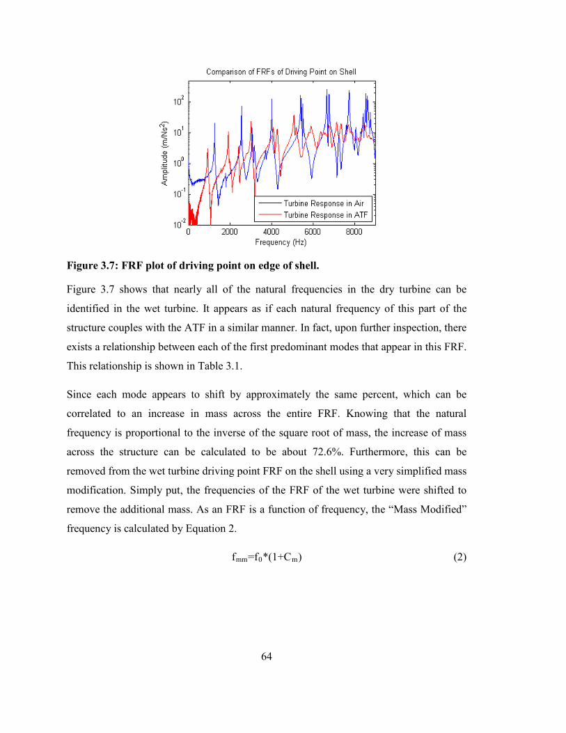
64

Figure 3.7: FRF plot of driving point on edge of shell.

Figure 3.7 shows that nearly all of the natural frequencies in the dry turbine can be

identified in the wet turbine. It appears as if each natural frequency of this part of the

structure couples with the ATF in a similar manner. In fact, upon further inspection, there

exists a relationship between each of the first predominant modes that appear in this FRF.

This relationship is shown in Table 3.1.

Since each mode appears to shift by approximately the same percent, which can be

correlated to an increase in mass across the entire FRF. Knowing that the natural

frequency is proportional to the inverse of the square root of mass, the increase of mass

across the structure can be calculated to be about 72.6%. Furthermore, this can be

removed from the wet turbine driving point FRF on the shell using a very simplified mass

modification. Simply put, the frequencies of the FRF of the wet turbine were shifted to

remove the additional mass. As an FRF is a function of frequency, the “Mass Modified”

frequency is calculated by Equation 2.

fmm=f0*(1+Cm) (2)

65

Table 3.1: This Table 3.is a comparison of the first six natural frequencies that appear in the FRFs of the driving point on the shell of the turbine.

Dry Fn (Hz)

Wet Fn (Hz) Change

2560 1921 -25.0% 4010 3020 -24.7% 5410 4095 -24.3% 5510 4286 -22.2% 6670 5081 -23.8% 6770 5195 -23.%

Mean -23.9% St Dev. 1.0%

In this equation, fmm is the modified frequency vector to be used by the FRF function, fo

is the original frequency vector, and Cm is the mean value of the change from Table 3.1.

The “Mass Modified” wet turbine FRF is shown with the dry turbine FRF in Figure 3.8.

Figure 3.8: Plot of FRFs of the dry turbine and the wet turbine. The wet turbine has had its frequency scaled in an attempt to remove the additional mass coupling caused by the fluid.

The FRFs of the dry turbine and the wet turbine at this driving point match up very well

after the modification. The amplitude of the peaks is not quite the same in both FRFs, and

66

some of the modes have disappeared, but it is hypothesized that this can be accounted for

by the additional damping caused by the coupling of the fluid with the structure, or that

those modes are coupling with the fluid differently than the primary modes shown here.

One of the causes for the difference in the amount of mass coupling in this structure

depending on the measurement location may have to do with the amount of surface area

that is in contact with the fluid with relation to the motion of the structure. Since the shell

is a large free surface area, the coupling of mass with that part of the structure is very

uniform and easy to predict. The blades, however, have a much smaller surface area,

along with more constrained boundary conditions which make the amount of surface area

in motion on that part of the structure more difficult to predict. It could be assumed that

the effective mass modification is then some function of the density of the liquid into

which the structure is submerged and some surface integral of the deformation of the

body

3.8 Conclusions Two methods of force input were presented. The ball bearing jig is very good for high

repeatability in quick tests on small structures. The major drawback of this test method

lies in the loss of phase data, and the limitation on the input points possible for testing

structures with this method. The ball bearing jig evolved into the impact rod jig, which

also has very good repeatability as well as accuracy of measurement. The impact rod also

has the advantage that it can be used on any part of a structure without worry of the

clearance needed for a ball bearing to avoid a double hit. The main disadvantage of the

impact rod is that it requires a lot of room for setup, and may not be feasible in tight

spaces.

Taking data on a structure that is fully submerged in a fluid has several challenges.

Precautions must be taken to ensure that the transducers used to make measurements are

working properly. The structure must be completely submerged in the fluid and free of

any air pockets that may cause errors in the measurements due to incorrect coupling of

the structure with the fluid.

67

After reviewing the data comparing the dry turbine to the wet turbine, several important

points can be made. Some parts of the turbine, like the shell, behave in a manner that

could easily be predicted when submerged in ATF due to a large surface area that is

allowed to move freely. The behavior of the blades seems to be a little more erratic when

comparing the wet turbine to the dry turbine FRF with regards to a more fixed point on

the structure, such as the turbine blades. As the blades are smaller and far more

constrained than the shell of the turbine, there is less effective mass added to that portion

of the structure. As a result, the effective mass coupling added by submersion into a fluid

is dependent on the amount of surface area of the structure that is both in motion and in

contact with the fluid.

3.9 References (1) Cakar O, Sanliturk KY. Elimination of Transducer Mass Loading Effects from

Frequency Response Functions. Science Direct Mechanical Systems and Signal Processing. 2005; Volume 19: pp. 87-104.

(2) Heylen W, Lammens S, Sas P. Excitation Considerations. Modal Analysis Theory and Testing, Katholieke Universiteit Leuven. 1997.

(3) Homm, Ehrlich J, Peine H, Wiesner H. Experimental and Numerical Investigation of a Complex Submerged Structure, Part I: Modal Analysis. Acta Acustica united with Acustica. 2003; Volume 89: pp. 61-70.

69

Chapter 4 – Characterizing Torque Converter Turbine Noise1

C. Walber1, J. Blough2, C. Anderson2, M. Johnson2, J, Schweitzer3

1PCB Piezotronics 3425 Walden Ave Depew, New York, USA 2 Michigan Technological University, Department of Mechanical Engineering 1400 Townsend Dr. Houghton, Michigan, USA 3 General Motors Powertrain Pontiac, Michigan, USA

4.1 Abstract As noise generated by other automotive components decreases, the noise generated by a

more compact torque converter has the potential to become more evident. It is therefore

important to characterize and understand any noise phenomena generated by the torque

converter. The research discussed in this paper concerns a specific noise event within the

torque converter that will be referred to as “turbine noise”. In some torque converters

operating at a high input torque, a high amplitude narrowband noise between 4 and 6 kHz

has been observed. The turbine noise appears to go away with the addition of notches to

the trailing edges of the turbine blades. It has been hypothesized that the turbine noise is

caused by Von Karman Vortex Shedding. The goal of this research was to determine the

source of the noise, to characterize the flow that set up the noise condition, and to

determine why trailing edge notches eliminate or reduce the noise. Several modifications

to the torque converter turbine were made to assess their effects on turbine noise.

Acoustic measurements were taken along with internal measurements of blade surface

acceleration, pressure and strain acquired through use of microwave telemetry. Analysis

1 The material contained in this chapter has been submitted to the Society for Experimental

Mechanics Journal: Experimental Techniques

70

of the test results confirmed that the characteristics of turbine noise follow the conditions

for Von Karman Vortex Shedding.

4.2 Introduction Torque Converter Operation - The automotive torque converter is the powertrain

component that multiplies engine torque to help launch the vehicle from a stop. It is a

hydrodynamic device which connects the engine to the transmission gears. As such it

absorbs torsional torque disturbances from the engine and allows the engine to idle

without requiring a separate mechanical clutch. Modern automotive torque converters are

made up of three elements, a mixed flow pump and turbine, and an axial flow stator.

Figure 4.1 is a basic schematic of a torque converter, including arrows showing the

direction of the toroidal flow induced during operation. Maximum efficiency is achieved

during high speed ratio operation while maximum torque multiplication is attained at

turbine speed equal to zero, commonly referred to as stall. Speed ratio (SR) is defined as

the ratio of the turbine speed to pump speed.

Figure 4.1: Cross section of an automotive torque converter; toroidal flow is indicated by the direction of the arrows with no tail. Arrows with tails indicate the normal cooling flow (1)

71

In the basic operation of a torque converter, the pump is driven by the engine through


Rotation of the pump imparts a centrifugal force on the automatic transmission fluid

(ATF). As depicted in Figure 4.1, this causes the fluid to flow from the inner radius of the

pump flow path to the outer radius where it is directed into the turbine. The turbine turns

the flow and directs it radially inward to the stator which guides the flow back into the

pump in a favorable angle with regards to pump operation. The flow through a bladed

element causes a change in the angular momentum of the fluid across the element which

results in a torque being applied to the shaft attached to that element. The turbine is

attached to the turbine shaft which is the input to the transmission gears. The stator shaft

is grounded through a one-way clutch to the transmission case, and stator torque is added

to pump torque. Summing the element torques through a free body analysis results in the

torque balance shown in Equation 1. Thus, the turbine torque, which is the output, is

greater than the pump torque, which is the input, and torque multiplication occurs.

(1)

When the torque converter is operating at high speed ratios, a clutch can be engaged to


hydrodynamic inefficiency of the torque converter.

4.3 Turbine Noise Torque Converter operational and performance parameters are generally viewed relative

to the speed ratio. For the particular torque converter geometry studied, a high amplitude

narrowband noise between 4 and 6 kHz occurs at operation with input torque above 300

Nm and speed ratio near 0.5. Other converters displayed a similar phenomenon at higher

torques and different frequencies. This turbine noise was detectable in the interior of

some early non-production development vehicles. After some research it was determined

that notching the trailing edge of the turbine blades reduced the noise to a level that could

not be detected. The noise is thought to be a result of a self–excited vibration

phenomenon known as Von Karman Vortex Shedding.

72

Some turbines are more susceptible to the noise phenomenon than others, possibly due to

variability in structural damping and acoustic transmissibility of the torque converter on

the whole. The sensitivity could be due to a combination of variability in turbine braze

quality, hub attachment, and blade trailing edge geometry. In addition, prior testing had

demonstrated that machined from solid turbines, and unbrazed turbines do not exhibit this

noise behavior. It was hypothesized that the turbine variations listed, along with adding

notches to blade trailing edges, alter either the structure of the turbine or the flow exiting

the turbine sufficiently to reduce or eliminate the noise phenomenon. As stated

previously, the root cause of the turbine noise phenomenon was thought to be Von

Karmen Vortex shedding. In this type of flow, the vortices couple with a natural

frequency of the turbine near the vortex frequency and cause a self–excited vibration,

resulting in the turbine shell being a sounding board for the turbine noise. Sound

measurements were taken of torque converters tested on a dynamometer that has a special

test fixture which contains acoustic treatments. Figure 4.2 shows the results depicted in a

frequency over speed ratio spectrogram for converters with turbines that contained blades

without and with notches on the trailing edges.

The turbine noise, circled in white, could be heard as a rather high pitched whistle over

the rest of the sound normally generated by the torque converter. The spectrograms in

Figure 4.2 clearly show that the addition of a notch to the trailing edge of the turbine

blades greatly diminishes the turbine noise.

73

Figure 4.2: Nearfield acoustic measurement of automotive torque converter equipped with an un-notched trailing edge turbine (Top) and a notched trailing edge turbine (Bottom) during simulated vehicle launch on dynamometer with an input torque of 350Nm. The area circled in white denotes the Turbine noise. Since the noise phenomenon is very narrow in the frequency domain, an indicator

function can be created using a bandpass filter. A sound pressure level (SPL) curve can

then be calculated and used to determine the presence of turbine noise as well as any

change in the noise over the course of various turbine alterations. The filter utilized is a

finite impulse response (FIR) type bandpass filter with a pass band from 3.5 kHz to 4.5

74

kHz. The resulting SPL curves in Figure 4.3 were created from the data shown in Figure

4.2.

Figure 4.3: Comparison of noise from an un-notched “Noisy” turbine and a notched quiet turbine during simulated vehicle launch with an input torque of 350Nm. The peak SPL of the un-notched turbine is over three times the peak SPL of the notched

turbine in Figure 4.3. The “noisy” range of this torque converter starts at around 0.5 SR

and continues up to 0.8 SR. It should be noted that these two tests are a comparison of

two different turbines. For the remaining tests, measurements were made on the same

turbine for a specific test before and after modifications to eliminate effects of part to part

variability. Because of this, several different turbines were used for the various tests.

Thus, a baseline unaltered turbine, is included with each experimental battery as a control

for that particular group.

4.4 Vortex Shedding and Vortex–induced Vibration The flow phenomenon suspected of being the source of turbine noise is Von Karman

vortex shedding. In Vortex shedding incidents, an unsteady flow occurs around bluff

bodies with specific fluid velocities. The flow past the object creates low pressure

75

vortices that alternate downstream of the object. Common structures on which vortices

can form include power cables, bridges, offshore pipelines, heat exchangers, and towers.

Figure 4.4 shows a side view of an airfoil in a transverse flow, with the alternating

vortices of light and dark gray.

Figure 4.4: Side view of an airfoil in a transverse flow causing a Von Karman Vortex Street.(3) Vortex shedding can occur in flows with Reynolds Numbers (Re) ranging from 47 to as

high as 107 (4). Re, a nondimensional description of velocity, is the product of free

stream velocity (U in mps) and characteristic length (D in meters), divided by kinematic

viscosity (ν in m2/s), shown in Equation 2.

(2)

Various geometries use different characteristic lengths for calculating Re. Characteristic

lengths for a sample of geometries are depicted in Figure 4.5. In this case Re is used in

conjunction with the dimensionless Strouhal (St) number to characterize oscillating

flows. Strouhal Number is an experimentally determined quantity for a given geometry

over a range of Re. It is generally constant over Re for a particular geometry, and

typically lies in the range of .1 to .3 for oscillating flow. The equation for Strouhal

Number is shown in Equation 3.

(3)

The parameters for Strouhal Number are the vortex frequency (f in Hz), the characteristic

length of the structure (D, in the case of a cylinder, the diameter in meters), and the free

stream velocity of the flow around the structure (U in mps, the same as U for the

76

Reynolds Number). The range of Strouhal Number over Reynolds Number for various

geometries is shown in Figure 4.5.

Figure 4.5: Strouhal Number for various geometries over Reynolds Number. (4) Ultimately, the Strouhal Number is a means of determining frequency of vortex release.

As each vortex sheds from the structure, the body will tend to move toward the low

pressure zone left in the wake of the vortex. Therefore, if the vortex frequency matches

close to a natural frequency of the structure, the structure can resonate and a self–excited

vibration can occur. This is called lock–in, and while the structure resonates at its natural

frequency the vortices shed at the natural frequency of the structure. The top portion of

Figure 4.6 shows a plot that tracks vortex frequency as it approaches the natural

frequency of the cylinder. Lock-in is the region in Figure 4.6 where the data points

indicating the vortex frequency begin to follow a horizontal line at a natural frequency of

the cylinder.

Once the vortex frequency is theoretically far enough away from the structure’s natural

frequency, the vortex frequency will part from the natural frequency as the interaction

between the structure and fluid becomes too weak to continue to support the feedback

required for the self-excited vibration. If no natural frequency is present, the vortex

frequency will remain near the “Stationary Cylinder Shedding Frequency” line indicated

in Figure 4.6. The motion of the cylinder (shown in the bottom portion of Figure 4.6) is

77

driving the vortex frequency (shown in the top portion of the figure) and vice versa. The

top vertical axis of Figure 4.6 is the dimensionless vortex frequency, with f, the natural

frequency of the system, normalizing fs, the vortex frequency. The lower plot shows the

amplitude of the motion of the cylinder, Ay, as it is normalized by the diameter of the

cylinder, D. The horizontal axis in both cases is the free stream velocity of the flow, U, as

it increases. U is normalized by the product of the natural frequency and the diameter of

the structure.

Figure 4.6: Vortex–induced vibration of a spring–supported, damped circular cylinder. ζ is the damping ratio of the structure. As seen in the two data sets, the lower the damping of the structure, the more motion caused by vortex lock-in, and the longer the vortices remain locked into the motion of the cylinder. (4) In the case of vortex lock-in for turbine noise, the free stream velocity is the toroidal flow

as it comes off of the trailing edge of the turbine blades. The characteristic length for use

in the Strouhal Number is a geometric feature normal to the direction of flow, possibly

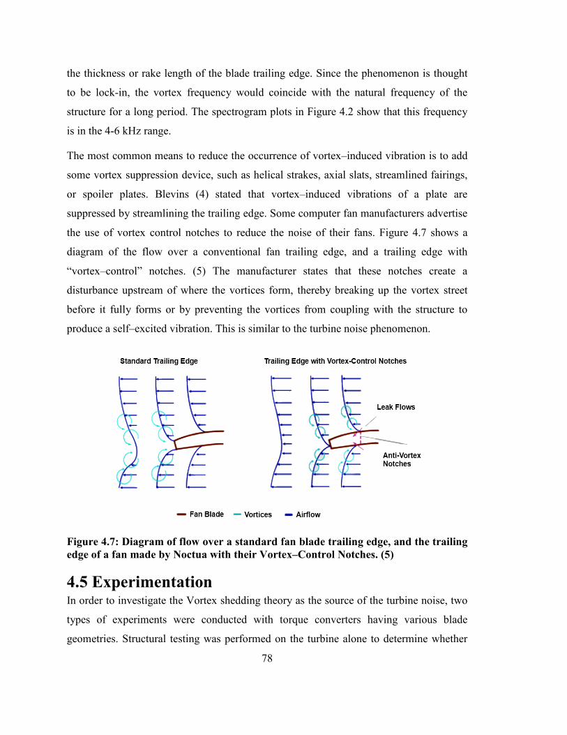
78

the thickness or rake length of the blade trailing edge. Since the phenomenon is thought

to be lock-in, the vortex frequency would coincide with the natural frequency of the

structure for a long period. The spectrogram plots in Figure 4.2 show that this frequency

is in the 4-6 kHz range.

The most common means to reduce the occurrence of vortex–induced vibration is to add

some vortex suppression device, such as helical strakes, axial slats, streamlined fairings,

or spoiler plates. Blevins (4) stated that vortex–induced vibrations of a plate are

suppressed by streamlining the trailing edge. Some computer fan manufacturers advertise

the use of vortex control notches to reduce the noise of their fans. Figure 4.7 shows a

diagram of the flow over a conventional fan trailing edge, and a trailing edge with

“vortex–control” notches. (5) The manufacturer states that these notches create a

disturbance upstream of where the vortices form, thereby breaking up the vortex street

before it fully forms or by preventing the vortices from coupling with the structure to

produce a self–excited vibration. This is similar to the turbine noise phenomenon.

Figure 4.7: Diagram of flow over a standard fan blade trailing edge, and the trailing edge of a fan made by Noctua with their Vortex–Control Notches. (5)

4.5 Experimentation In order to investigate the Vortex shedding theory as the source of the turbine noise, two

types of experiments were conducted with torque converters having various blade

geometries. Structural testing was performed on the turbine alone to determine whether

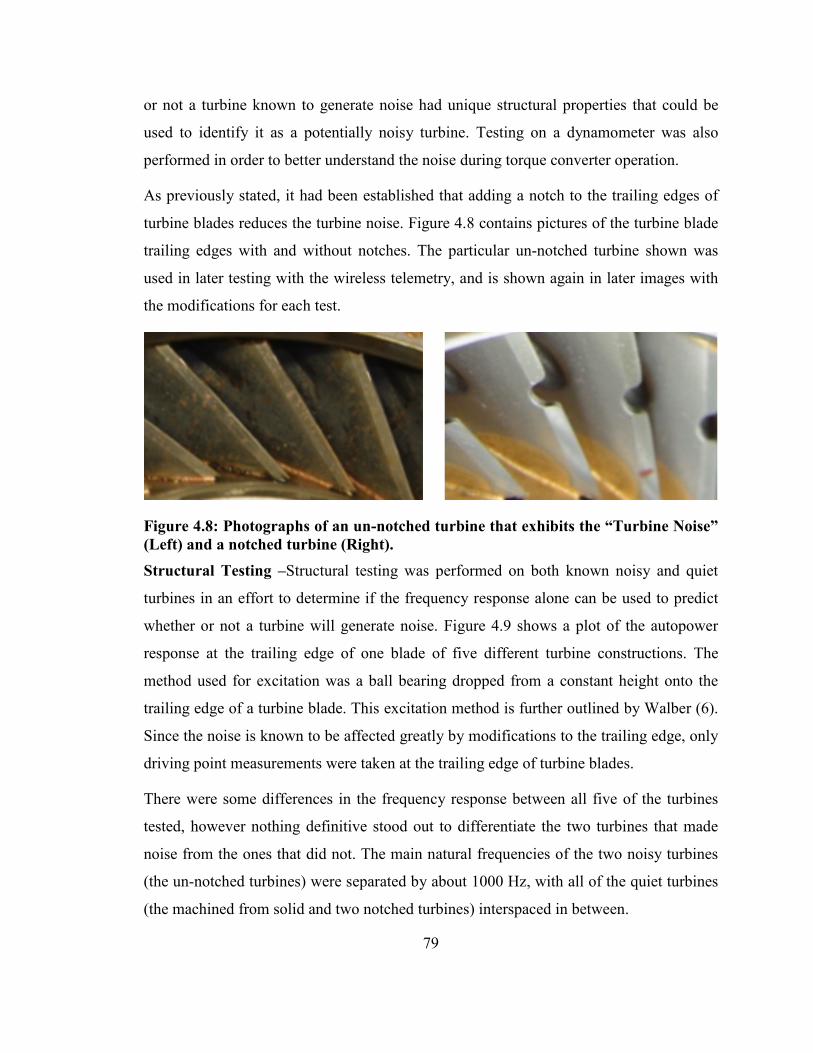
79

or not a turbine known to generate noise had unique structural properties that could be

used to identify it as a potentially noisy turbine. Testing on a dynamometer was also

performed in order to better understand the noise during torque converter operation.

As previously stated, it had been established that adding a notch to the trailing edges of

turbine blades reduces the turbine noise. Figure 4.8 contains pictures of the turbine blade

trailing edges with and without notches. The particular un-notched turbine shown was

used in later testing with the wireless telemetry, and is shown again in later images with

the modifications for each test.

Figure 4.8: Photographs of an un-notched turbine that exhibits the “Turbine Noise” (Left) and a notched turbine (Right). Structural Testing –Structural testing was performed on both known noisy and quiet

turbines in an effort to determine if the frequency response alone can be used to predict

whether or not a turbine will generate noise. Figure 4.9 shows a plot of the autopower

response at the trailing edge of one blade of five different turbine constructions. The

method used for excitation was a ball bearing dropped from a constant height onto the

trailing edge of a turbine blade. This excitation method is further outlined by Walber (6).

Since the noise is known to be affected greatly by modifications to the trailing edge, only

driving point measurements were taken at the trailing edge of turbine blades.

There were some differences in the frequency response between all five of the turbines

tested, however nothing definitive stood out to differentiate the two turbines that made

noise from the ones that did not. The main natural frequencies of the two noisy turbines

(the un-notched turbines) were separated by about 1000 Hz, with all of the quiet turbines

(the machined from solid and two notched turbines) interspaced in between.

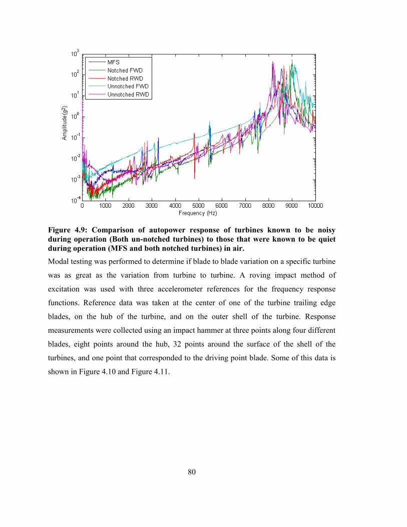
80

Figure 4.9: Comparison of autopower response of turbines known to be noisy during operation (Both un-notched turbines) to those that were known to be quiet during operation (MFS and both notched turbines) in air. Modal testing was performed to determine if blade to blade variation on a specific turbine

was as great as the variation from turbine to turbine. A roving impact method of

excitation was used with three accelerometer references for the frequency response

functions. Reference data was taken at the center of one of the turbine trailing edge

blades, on the hub of the turbine, and on the outer shell of the turbine. Response

measurements were collected using an impact hammer at three points along four different

blades, eight points around the hub, 32 points around the surface of the shell of the

turbines, and one point that corresponded to the driving point blade. Some of this data is

shown in Figure 4.10 and Figure 4.11.

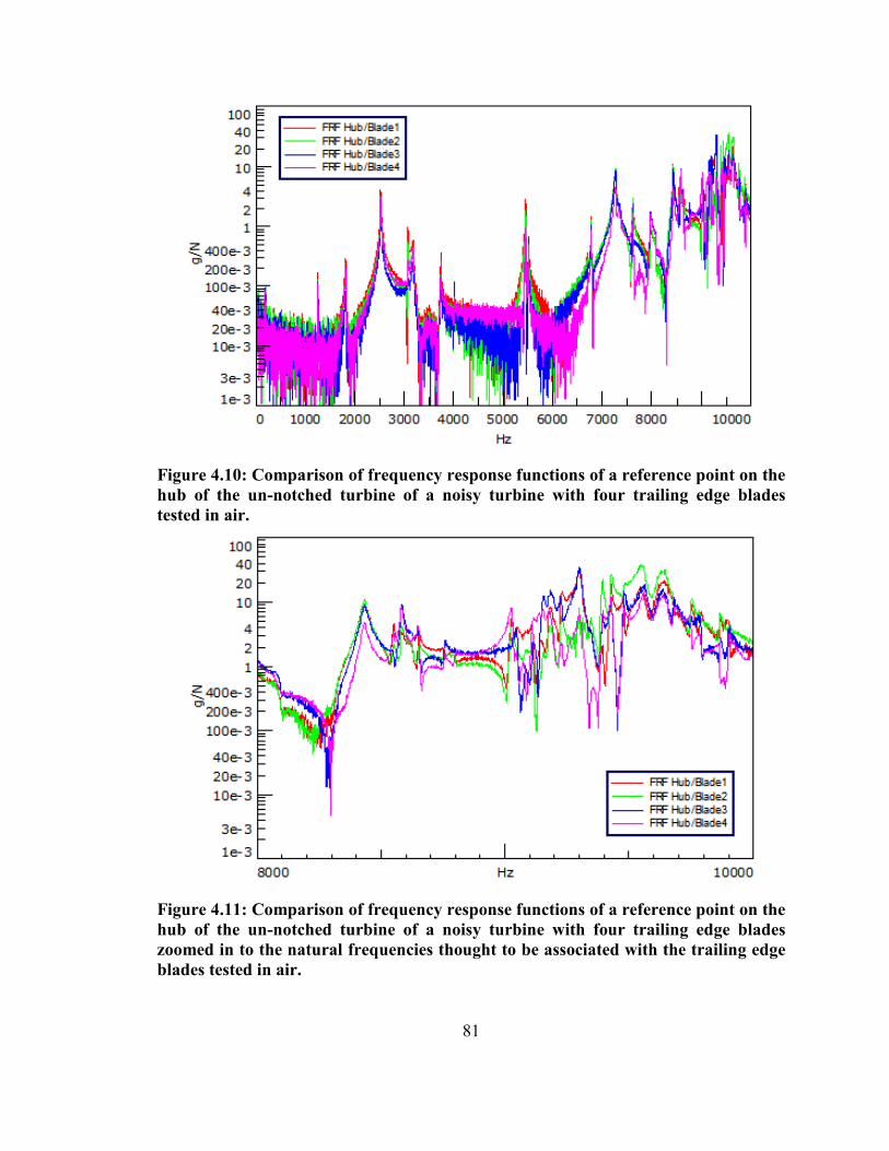
81

Figure 4.10: Comparison of frequency response functions of a reference point on the hub of the un-notched turbine of a noisy turbine with four trailing edge blades tested in air.

Figure 4.11: Comparison of frequency response functions of a reference point on the hub of the un-notched turbine of a noisy turbine with four trailing edge blades zoomed in to the natural frequencies thought to be associated with the trailing edge blades tested in air.

82

Figure 4.10 shows that each blade has a very small variation with respect to the others

when the hub is used as a frequency response reference point and looking at the entire

frequency range. However, Figure 4.11 shows what is believed to be the individual

natural frequencies associated with each turbine blade. It is apparent from review of the

Figure 4.that it would be difficult to use variation of individual blade frequencies to

determine whether or not a turbine is noisy. In addition, there does not appear to be a

natural frequency at 4 kHz, the frequency at which the turbine noise occurs. However,

this data was taken in air, which is not the normal operating medium for the torque

converter.

The vibration mode of the turbine at the frequency of the noise in the operating medium,

ATF, was investigated next. Only one turbine, an un-notched turbine, was tested both in

and out of ATF since it was already determined that it could not easily be differentiated

dynamically from a notched turbine or other quiet turbines. The same physical points on

the structure were measured when the turbine was placed in ATF as when it was in air.

The data from the submerged testing is shown in Figure 4.12. The physical points

referenced on the turbine where the data was measured are identical to those measured in

Figure 4.10. The comparison between test results in air and in ATF shows that the natural

frequencies of the turbine in ATF shift almost uniformly to lower frequencies, while the

overall amplitude of the data remains about the same. This indicates that the addition of

ATF to the turbine acts as mass loading with regards to vibration, while very little

damping can be detected here. As can be seen in the peaks shown in Figure 4.12, the shift

in the natural frequencies placed one resonance right at 4 kHz and a second resonance at

around 4.3 kHz.

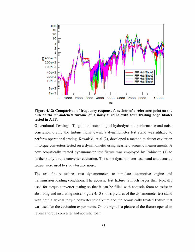
83

Figure 4.12: Comparison of frequency response functions of a reference point on the hub of the un-notched turbine of a noisy turbine with four trailing edge blades tested in ATF. Operational Testing – To gain understanding of hydrodynamic performance and noise

generation during the turbine noise event, a dynamometer test stand was utilized to

perform operational testing. Kowalski, et al (2), developed a method to detect cavitation

in torque converters tested on a dynamometer using nearfield acoustic measurements. A

new acoustically treated dynamometer test fixture was employed by Robinette (1) to

further study torque converter cavitation. The same dynamometer test stand and acoustic

fixture were used to study turbine noise.

The test fixture utilizes two dynamometers to simulate automotive engine and

transmission loading conditions. The acoustic test fixture is much larger than typically

used for torque converter testing so that it can be filled with acoustic foam to assist in

absorbing and insulating noise. Figure 4.13 shows pictures of the dynamometer test stand

with both a typical torque converter test fixture and the acoustically treated fixture that

was used for the cavitation experiments. On the right is a picture of the fixture opened to

reveal a torque converter and acoustic foam.

84

Figure 4.13: Left: Comparison of original torque converter dynamometer test fixture (Red) and acoustic test fixture (Gray). Right: Close up of opened acoustic test stand with acoustic foam. (1) Test Procedure - For turbine noise testing, a standard dynamometer test procedure was

developed to emulate torque converter performance during vehicle takeoff. The

dynamometer test starts with a warm up and stabilization cycle. Then, the individual

experiments begin with the torque converter pump being spun up to a specified constant

torque. The turbine is rotated at a constant 500 RPM during this spin–up phase of the

pump. Once the pump torque has settled out, the turbine is accelerated at a rate of 50

RPM/s to a speed of 3000 RPM. During the test, all speeds, torques, pressures,

temperatures, and flow rates are collected via the control system at a 10 Hz sample rate.

Nearfield acoustic measurements are taken at a 51.2 kHz sample rate. Pump and turbine

speeds are also measured at 51.2 kHz so that some reference may be made between the

acoustic data and other test parameters. After a test is completed, a torque correction

factor which includes dynamic torque losses due to the inertia of the entire dynamometer

system is applied to the measured torques.

For most of the tests outlined in this paper, a suite of turbine data was acquired in

addition to nearfield acoustic data. This included trailing edge blade acceleration, strain,

and surface pressure data.

Dynamometer Tests - The turbine noise was known to be a high input torque

phenomenon. To better understand the torque influence, an investigation was conducted

to identify the effect of the input torque on the generated noise. Figure 4.14 is a waterfall

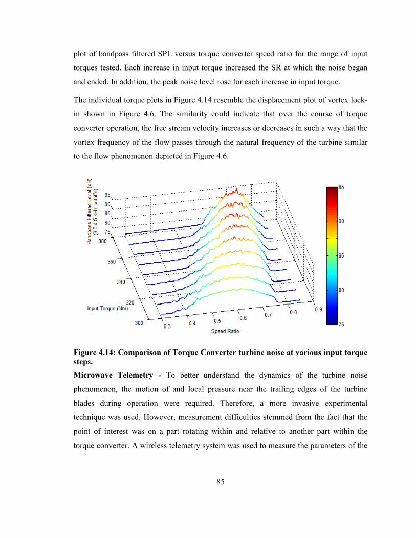
85

plot of bandpass filtered SPL versus torque converter speed ratio for the range of input

torques tested. Each increase in input torque increased the SR at which the noise began

and ended. In addition, the peak noise level rose for each increase in input torque.

The individual torque plots in Figure 4.14 resemble the displacement plot of vortex lock-

in shown in Figure 4.6. The similarity could indicate that over the course of torque

converter operation, the free stream velocity increases or decreases in such a way that the

vortex frequency of the flow passes through the natural frequency of the turbine similar

to the flow phenomenon depicted in Figure 4.6.

Figure 4.14: Comparison of Torque Converter turbine noise at various input torque steps. Microwave Telemetry - To better understand the dynamics of the turbine noise

phenomenon, the motion of and local pressure near the trailing edges of the turbine

blades during operation were required. Therefore, a more invasive experimental

technique was used. However, measurement difficulties stemmed from the fact that the

point of interest was on a part rotating within and relative to another part within the

torque converter. A wireless telemetry system was used to measure the parameters of the

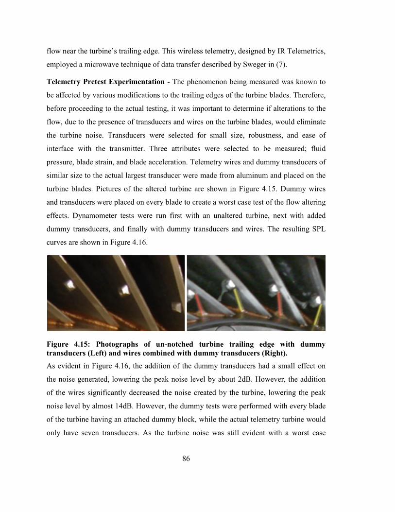
86

flow near the turbine’s trailing edge. This wireless telemetry, designed by IR Telemetrics,

employed a microwave technique of data transfer described by Sweger in (7).

Telemetry Pretest Experimentation - The phenomenon being measured was known to

be affected by various modifications to the trailing edges of the turbine blades. Therefore,

before proceeding to the actual testing, it was important to determine if alterations to the

flow, due to the presence of transducers and wires on the turbine blades, would eliminate

the turbine noise. Transducers were selected for small size, robustness, and ease of

interface with the transmitter. Three attributes were selected to be measured; fluid

pressure, blade strain, and blade acceleration. Telemetry wires and dummy transducers of

similar size to the actual largest transducer were made from aluminum and placed on the

turbine blades. Pictures of the altered turbine are shown in Figure 4.15. Dummy wires

and transducers were placed on every blade to create a worst case test of the flow altering

effects. Dynamometer tests were run first with an unaltered turbine, next with added

dummy transducers, and finally with dummy transducers and wires. The resulting SPL

curves are shown in Figure 4.16.

Figure 4.15: Photographs of un-notched turbine trailing edge with dummy transducers (Left) and wires combined with dummy transducers (Right). As evident in Figure 4.16, the addition of the dummy transducers had a small effect on

the noise generated, lowering the peak noise level by about 2dB. However, the addition

of the wires significantly decreased the noise created by the turbine, lowering the peak

noise level by almost 14dB. However, the dummy tests were performed with every blade

of the turbine having an attached dummy block, while the actual telemetry turbine would

only have seven transducers. As the turbine noise was still evident with a worst case

87

dummy transducer/wire combination, it was determined that the telemetry testing could

proceed.

Figure 4.16: SPL plot comparing test alterations to turbine trailing edge. The fact that the turbine noise diminished with the presence of dummy transducers and

wires is in line with the vortex shedding hypothesis. According to Blevins (5), creating

some disturbance in the flow field near the point where vortices form prevents them from

coupling with the structure. This could be why the noise is reduced but not completely

eliminated by the transducer wires. The resulting alteration to flow is not large enough to

either eliminate the vortices or completely decouple them from the structure.

Microwave Telemetry Preparation – Several modifications to the existing torque

converter assembly were required for installation and operation of the telemetry system.

Since a torque converter is completely housed inside of a metal shell, creating a

Faraday’s Cage, an opening in the metal is required to allow the transmission of the

microwaves to the receivers. A polycarbonate extension ring for a bolt together torque

converter was designed to provide an outlet path for microwave transmission. The ring,

shown in Figure 4.17, permits the microwaves to travel from the transmitter inside the

torque converter to the external receiver. A second function of the polycarbonate

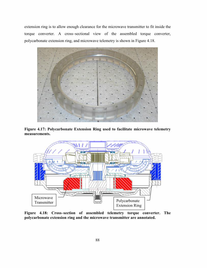
88

extension ring is to allow enough clearance for the microwave transmitter to fit inside the

torque converter. A cross–sectional view of the assembled torque converter,

polycarbonate extension ring, and microwave telemetry is shown in Figure 4.18.

Figure 4.17: Polycarbonate Extension Ring used to facilitate microwave telemetry measurements.

Figure 4.18: Cross–section of assembled telemetry torque converter. The polycarbonate extension ring and the microwave transmitter are annotated.

Microwave Transmitter Polycarbonate

Extension Ring

89

4.6 Analysis Telemetry Data Analysis – Figure 4.19 shows accelerometer data measured at the

trailing edge of a turbine blade from a SR test with 350 Nm input torque. The top plot

contains measurements from the un-notched turbine and the bottom plot from the notched

turbine. A clear band of motion at 4 kHz is shown for both sets of data. However, the

amount of motion is much greater on the un-notched turbine (ten times greater). This

indicates that at the frequency of interest, the trailing edge of the turbine is indeed

moving, and could be the source of the noise. With respect to Vortex shedding, recall that

the impact data demonstrated that a natural frequency of the turbine blades exists at 4

kHz for both the notched and un-notched turbines in ATF. This means that the notch

affects the flow in some way other than modifying the structural parameters of the

turbine’s trailing edge, and that blade motion occurs at a natural frequency for both

turbines. The fact that the disturbance occurs at a natural frequency is a characteristic of

vortex shedding with lock-in. With the notched turbine, the excitation is just not great

enough to be detected.

For Figure 4.19 through 21, the responses are plotted in Decibels (dB) to allow the data to

better stand out and facilitate data comparisons. The decibel values are simply the log of

the value measured divided by some reference value. In the cases of acceleration, fluid

pressure, and strain, the reference values used were 20 µm/s2, 2e-5 psi, and 2e-5 µstrain

respectively.

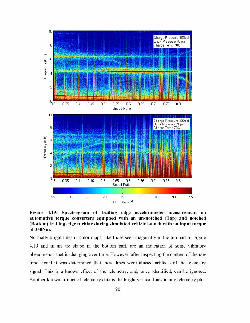
90

Figure 4.19: Spectrogram of trailing edge accelerometer measurement on automotive torque converters equipped with an un-notched (Top) and notched (Bottom) trailing edge turbine during simulated vehicle launch with an input torque of 350Nm. Normally bright lines in color maps, like those seen diagonally in the top part of Figure

4.19 and in an arc shape in the bottom part, are an indication of some vibratory

phenomenon that is changing over time. However, after inspecting the content of the raw

time signal it was determined that these lines were aliased artifacts of the telemetry

signal. This is a known effect of the telemetry, and, once identified, can be ignored.

Another known artifact of telemetry data is the bright vertical lines in any telemetry plot.

91

These lines are a result of signal dropouts that occur from a poor signal path or excess

noise at the telemetry carrier frequency, and can also be ignored.

Figure 4.20 and Figure 4.21 show the trailing edge fluid pressure response and blade

strain at 350 Nm input torque of the un-notched and notched turbines, respectively top

and bottom. As with the accelerometer measurements, the pressure fluctuation and strain

around 4 kHz are evident in the un-notched turbine. In the notched turbine no pressure

fluctuation is detectable above the background noise, while only minimal strain is

observed. These results also follow the vortex induced vibration hypothesis. The minimal

strain and absence of pressure fluctuations could mean that the addition of notches

prevents the flow from forming vortices about the trailing edge of the turbine.

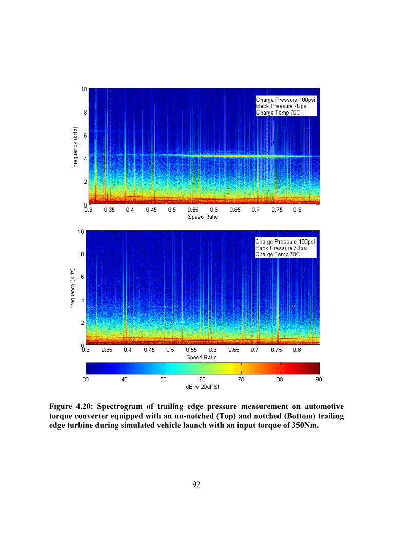
92

Figure 4.20: Spectrogram of trailing edge pressure measurement on automotive torque converter equipped with an un-notched (Top) and notched (Bottom) trailing edge turbine during simulated vehicle launch with an input torque of 350Nm.

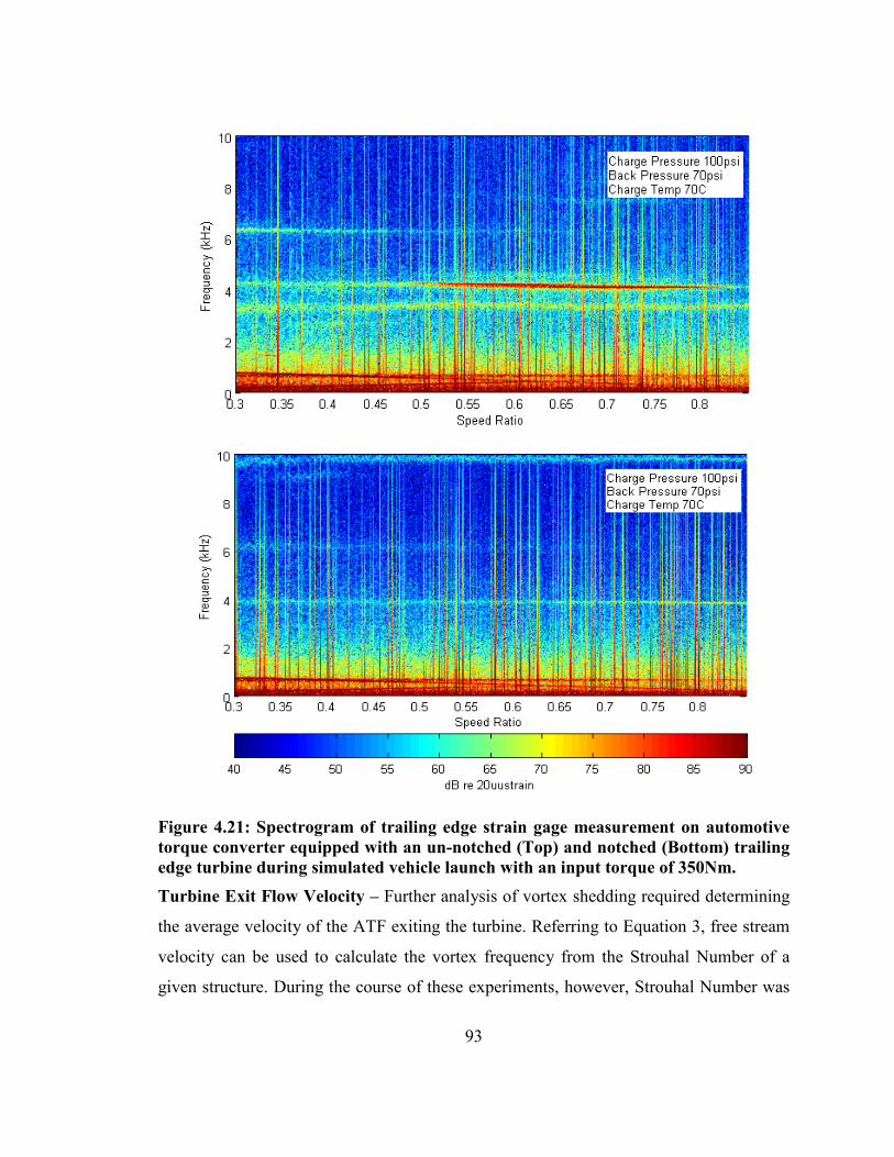
93

Figure 4.21: Spectrogram of trailing edge strain gage measurement on automotive torque converter equipped with an un-notched (Top) and notched (Bottom) trailing edge turbine during simulated vehicle launch with an input torque of 350Nm. Turbine Exit Flow Velocity – Further analysis of vortex shedding required determining

the average velocity of the ATF exiting the turbine. Referring to Equation 3, free stream

velocity can be used to calculate the vortex frequency from the Strouhal Number of a

given structure. During the course of these experiments, however, Strouhal Number was

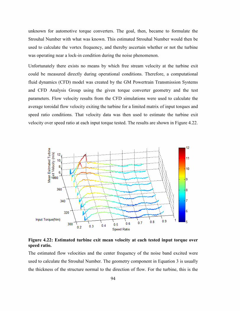
94

unknown for automotive torque converters. The goal, then, became to formulate the

Strouhal Number with what was known. This estimated Strouhal Number would then be

used to calculate the vortex frequency, and thereby ascertain whether or not the turbine

was operating near a lock-in condition during the noise phenomenon.

Unfortunately there exists no means by which free stream velocity at the turbine exit

could be measured directly during operational conditions. Therefore, a computational

fluid dynamics (CFD) model was created by the GM Powertrain Transmission Systems

and CFD Analysis Group using the given torque converter geometry and the test

parameters. Flow velocity results from the CFD simulations were used to calculate the

average toroidal flow velocity exiting the turbine for a limited matrix of input torques and

speed ratio conditions. That velocity data was then used to estimate the turbine exit

velocity over speed ratio at each input torque tested. The results are shown in Figure 4.22.

Figure 4.22: Estimated turbine exit mean velocity at each tested input torque over speed ratio. The estimated flow velocities and the center frequency of the noise band excited were

used to calculate the Strouhal Number. The geometry component in Equation 3 is usually

the thickness of the structure normal to the direction of flow. For the turbine, this is the

95

blade trailing edge thickness. A Strouhal Number of 0.28 was calculated and was

assumed to be constant across all of the tested conditions. This fits very well in the range

of known Strouhal Numbers for existing geometries. The top curve in Figure 4.23 shows

a plot of the resulting vortex frequency curve versus SR calculated from the estimated

turbine exit velocities using 0.28 as the Strouhal Number, and using 0.6mm as the

characteristic length. The lower curve in Figure 4.23 is the filtered sound pressure level

curve from the 350 Nm input torque test. As speed ratio increases and the vortex

frequency nears 4 kHz, the noise begins to develop (this occurs at about 0.5 SR). The

vortex frequency continues down to just below 3.5 kHz and stays constant through the

rest of the experiment. A frequency of 3.5 kHz might be just far enough away from the

natural frequency of the structure that the vortices begin to decouple and allow the noise

to dissipate, similar to the lock-in flow phenomenon depicted in Figure 4.6.

Figure 4.23: Plots of estimated vortex frequency (Top) and filtered sound pressure level (Bottom) over speed ratio. The noise data was taken during simulated vehicle launch testing on dynamometer with an input torque of 350Nm. The vortex frequency was calculated using the turbine exit velocity curve for 350Nm, a trailing edge thickness of .6mm, and a Strouhal Number of .28 over the entire test. It is interesting to note that the exit flow velocity, and therefore the vortex frequency, of

the turbine do not vary much once the onset of the noise occurs. This could explain why

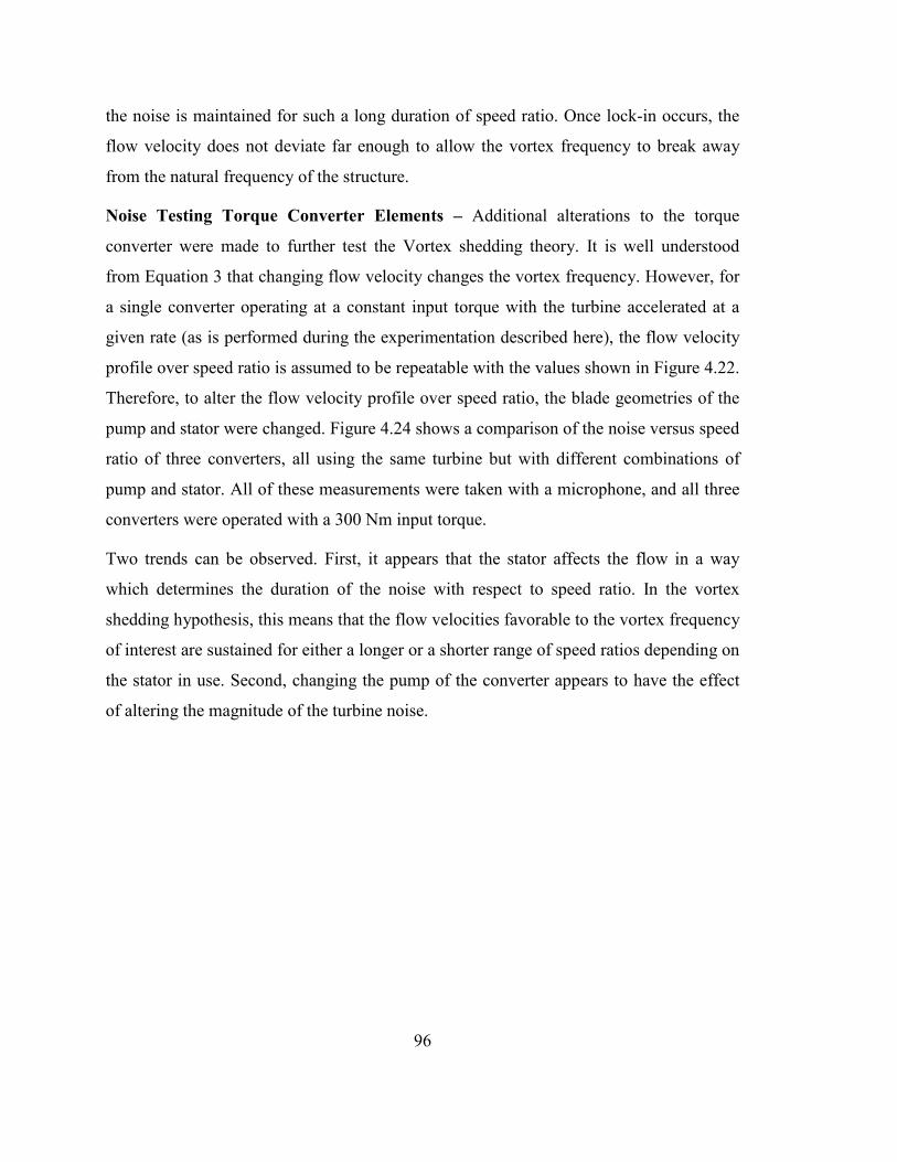
96

the noise is maintained for such a long duration of speed ratio. Once lock-in occurs, the

flow velocity does not deviate far enough to allow the vortex frequency to break away

from the natural frequency of the structure.

Noise Testing Torque Converter Elements – Additional alterations to the torque

converter were made to further test the Vortex shedding theory. It is well understood

from Equation 3 that changing flow velocity changes the vortex frequency. However, for

a single converter operating at a constant input torque with the turbine accelerated at a

given rate (as is performed during the experimentation described here), the flow velocity

profile over speed ratio is assumed to be repeatable with the values shown in Figure 4.22.

Therefore, to alter the flow velocity profile over speed ratio, the blade geometries of the

pump and stator were changed. Figure 4.24 shows a comparison of the noise versus speed

ratio of three converters, all using the same turbine but with different combinations of

pump and stator. All of these measurements were taken with a microphone, and all three

converters were operated with a 300 Nm input torque.

Two trends can be observed. First, it appears that the stator affects the flow in a way

which determines the duration of the noise with respect to speed ratio. In the vortex

shedding hypothesis, this means that the flow velocities favorable to the vortex frequency

of interest are sustained for either a longer or a shorter range of speed ratios depending on

the stator in use. Second, changing the pump of the converter appears to have the effect

of altering the magnitude of the turbine noise.

97

Figure 4.24: SPL plot comparing noise level in converters with different stator and pump combinations. Each of the tests shown was run at 300 Nm input torque. Turbine Blade Trailing Edge Thickness - Following Equation 3 once again, altering

the characteristic length of the geometry hypothesized to be creating the vortices should

also alter the vortex frequency. For this experiment, another turbine was selected and

tested for turbine noise. The blade trailing edges of this turbine were then ground thinner

to a thickness where the vortex frequency was expected to interact with a higher turbine

natural frequency and create a similar noise at the new frequency.

Figure 4.25, shows the sound pressure level color maps from testing the un-notched

turbine and testing the same turbine after the trailing edge modification. It is evident that

making the trailing edge thinner did indeed alter the noise, but by eliminating it instead of

changing its frequency. One possibility for the noise disappearance could be that even if

the vortices are still occurring at the higher vortex frequency, they might not couple with

a vibration mode of the turbine to excite it acoustically. The disturbance therefore would

be undetectable with the microphone.

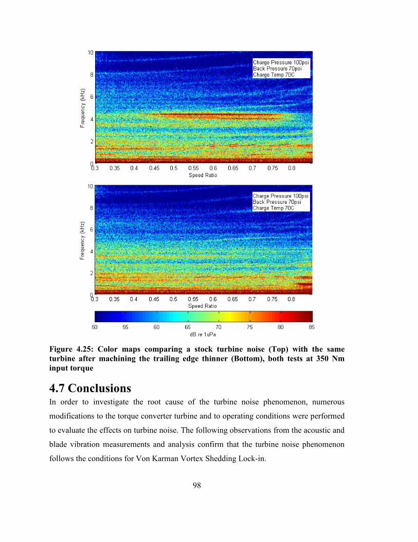
98

Figure 4.25: Color maps comparing a stock turbine noise (Top) with the same turbine after machining the trailing edge thinner (Bottom), both tests at 350 Nm input torque

4.7 Conclusions In order to investigate the root cause of the turbine noise phenomenon, numerous

modifications to the torque converter turbine and to operating conditions were performed

to evaluate the effects on turbine noise. The following observations from the acoustic and

blade vibration measurements and analysis confirm that the turbine noise phenomenon

follows the conditions for Von Karman Vortex Shedding Lock-in.

99

• Acoustic and vibration measurements show that turbine noise was generated at a

frequency between 3.5 and 4.5 kHz. Impact testing of the turbine in ATF showed a

natural frequency near 4 kHz. The close match of frequencies supports a Vortex

Shedding Lock-in condition.

• Increasing input torque results in an upward shift of the turbine noise relative to speed

ratio and in higher noise levels. The change in free stream velocity exiting the turbine

that results from the change in input torque alters the Strouhal Number and the

proximity of vortex frequency to turbine natural frequency. The resulting noise versus

input torque and speed ratio pattern resembles the lock-in and release pattern of

Vortex Shedding.

• Acoustic measurements and turbine blade measurements for acceleration, strain, and

pressure confirmed that altering the trailing edge of a noisy turbine either reduces or

completely eliminates the noise. The blade geometry modifications from the notch

and telemetry transducers alter the flow enough to reduce or eliminate the vortices or

decouple them from the structure. The effect is similar to claims made for vortex

suppression features added to other types of turbomachinery such as computer fans.

• Free stream velocities (and thus Strouhal number and vortex frequency) were

modified by testing several combinations of pumps and stators. Similar to changing

input torque, the alterations to pump and stator blade geometries either shifted the

noise duration with respect to torque converter speed ratio, or changed the level of

noise.

• The structure characteristic length for Strouhal number was changed by reducing the

turbine trailing edge thickness. The modified Strouhal number was expected to shift

the vortex frequency and turbine noise to a higher turbine natural frequency. The fact

that the noise was eliminated instead could mean that the vortices could not couple

with a turbine mode to excite it acoustically.

• The value of Strouhal number for the turbine noise phenomenon was estimated from

CFD simulations of free stream velocity exiting the turbine for a range of operating

conditions. The resulting estimate was a constant of 0.28 which fits well with known

Strouhal Numbers of other similar geometries. The estimated Strouhal Number was

100

subsequently used to calculate turbine vortex frequency versus speed ratio. The

results in Figure 4.23 show that the onset of the noise coincided with vortex

frequency passing near 4 kHz. Therefore, the simulated characteristics of flow exiting

the turbine during the turbine noise phenomenon follow requirements for vortex lock-

in.

Acknowledgement The writers would like to thank Ibraheem Shaik from the GM Powertrain Systems and

CFD Analysis Group for his contribution of CFD simulations used to estimate torque

converter flow velocities at the turbine exit.

4.8 References (1) Robinette DL. Detecting and Predicting the onset of Cavitation in Automotive Torque

Converters. PhD Dissertation, Michigan Technological University. Ann Arbor: ProQuest/UMI. 2007.

(2) Kowalski D, Anderson CL, Blough JR. Cavitation Detection in Automotive Torque Converters Using Nearfield Acoustical Measurements. SAE-NVH. 5/16/2005; 2005–01– 2516.


(4) Blevins R. Flow Induced Vibration. Krieger Publishing Company. 2001.

(5) Noctua Fan Company. Nine Blade Design with Vortex-Control Notches. 2012; http://www.noctua.at/main.php?show=nine_blade_design&lng=en.

(6) Walber C, Blough JR, Anderson CL, Johnson MA. Measuring and Comparing Frequency Response Functions of Torque Converter Turbines Submerged In Transmission Fluid. SAE-NVH. 5/17/2011; 2011-01-1662.

(7) Sweger P, Anderson CL, Blough JR. Measurements of Strain on 310 Mm Converter Turbine Blade. International Journal of Rotating Machinery. 2004; Volume 10, No 1: pp. 55-63.

(8) Mekkes J, Anderson CL, Narain A. Static Pressure Measurements and Cavitation Signatures on the Nose of a Torque Convertor’s Stator Blade. ISROMAC. 2004.

(9) Robinette DL, Schweitzer JM, Maddock DG, Anderson CL, Blough JR, Johnson MA. Predicting the Onset of Cavitation in Automotive Torque Converters—Part I: Designs with Geometric Similitude. International Journal of Rotating Machinery. 2008; Article ID 803940.

101

Chapter 5 – Conclusions

This chapter will discuss the findings of the two primary projects, desinent cavitation

detection during vehicle launch and the turbine noise phenomenon. Several

recommendations will be made with regards to torque converter research in general.

5.1 Experimental Desinent Cavitation Conclusions The observations made with relation to desinent cavitation are based on nearfield acoustic

measurements and analysis collected during constant input torque turbine speed sweeps.

The findings of this study are summarized here:

1) A dimensionless group created from the product of dimensionless input torque and

speed ratio was selected as the dimensionless response in an effort to be able to relate

both quantities to the torque converter design parameters as well as the varying

operating conditions during vehicle launch. This quantity was named dimensionless

rotational power.

2) Increasing charge pressure and decreasing the temperature of the cooling flow

reduces the duration of cavitation occurring in the torque converter; that is by ending

cavitation at a lower speed ratio. This is in accordance with the stall cavitation

relation.

3) Increasing torque input to the torque converter increases the duration of cavitation.

4) The response surface models that were created based on the converters having similar

geometric properties (Torus aspect ratio) or similar operating capacities (Unit input

speed) are capable of predicting the dimensionless rotational power of the converter

at the point of desinent cavitation within a %RMSE of 10.8 and 11.6 percent

respectively.

5) The general model developed from test results for all the converters tested is capable

of predicting dimensionless rotational power at desinent cavitation with a 14.4

%RMSE.

102

5.2 Turbine Noise Study Conclusions A summary of the discoveries made during the turbine noise study are listed below.

1) Some turbines are more susceptible to the noise phenomenon than others. It is

believed that the sensitivity is due to a combination of braze quality, hub attachment,

and trailing edge finish and thickness.

2) The turbine noise shifts to higher speed ratios when a higher input torque is applied.

3) Altering the trailing edge of a turbine which is noisy either reduces the noise or

eliminates it completely. This includes the addition of trip wires, notches, dummy

blocks, as well as altering the taper at the trailing edge of the turbine.

4) Some turbines generate the noise when paired with some stator and pump

combinations, but not in others.

5) The frequency at which the noise occurs does not shift with any of the alterations

discussed in the previous conclusions.

6) Based on previous conclusions, it is believed that vortex shedding is the most likely

cause of the noise phenomenon. The frequency at which the vortices form relates very

closely to both a natural frequency of the turbine trailing edge blades as well as the

estimated vortex frequency during that point of torque converter operation.

7) Thus far it has been impossible to determine by measuring frequency response or any

other static non-operating tests whether or not a turbine will be noisy or quiet.

5.3 General Automotive Torque Converter Recommendations The study discussed here has raised some additional questions that require additional

research to fully understand. The following list contains work that is recommended to be

done in the future to better understand automotive torque converters in general, as well as

the two primary investigations discussed here.

1) Create a bench-top test to perform flow measurements on portions of torque converter

elements to understand the flow interactions inside the individual passages of each

specific element (pump, stator, and turbine). These experiments should take into

103

account not only flow speed, but also angle of attack of the flow on the leading edge

of the blades of that particular element.

2) As a part of a bench-top turbine test, determine if Von-Karman Vortices can be seen

shedding off of the trailing edges of the turbine blades.

3) Select one torque converter where the operational parameters are very well known,

and perform a full vehicle launch simulation, including transmission shifts and

throttle adjustments, using the dynamometer test stand and correlate the findings to

actual vehicle launch data. Include nearfield acoustic measurements in both

experiments.

4) Develop a full computational fluid dynamics (CFD) model of the flow inside the

torque converter. This model should be correlated to not only steady state torque

converter testing, but also speed sweep data and the testing performed in the bench-

top experiment mentioned previously. If possible, a multiphase flow simulation

should be included in this model in order to further increase understanding of

cavitation and its effect on the operation of the torque converter.

5) Develop and perform a flow visualization experiment on an entire automotive torque

converter assembly. The CFD model should also be correlated to the bench-top

experimentation to be sure that all information garnered from the model is as accurate

as possible.

6) Perform a full transfer path analysis on the torque converter-flex shaft-crank shaft

vibration path during simulated operation. Use both axial force transducers and in line

torque cells at each interface to measure the forces actually being imparted on the

engine by the torque converter.

7) Perform more clutch engagement experimentation. Include clutch engagement in the

transfer path analysis already discussed, but also include acoustic measurements

during the experiment to determine if locking the clutch creates additional noise. This

may be more important with the advent of launch converters as clutch chatter may

become more prevalent.

105

References

(1) Robinette DL. Detecting and Predicting the onset of Cavitation in Automotive Torque Converters. PhD Dissertation, Michigan Technological University. Ann Arbor: ProQuest/UMI. 2007.

(2) Arakeri V. Cavitation Inception. Proc. Indian Acad. Sci. 1979; Vol. C2, Pt. 2: pp.

149-177. (3) Mekkes J, Anderson CL, Narain A. Static Pressure Measurements on the Nose of a

Torque Converter Stator during Cavitation. ISROMAC. 2004. (4) Zeng L, Anderson CL, Sweger PO, Narain A. Experimental Investigation of

Cavitation Signatures in an Automotive Torque Converter Using a Microwave Telemetry Technique. ISORMAC. 2002.

(5) Blander M, Katz JL. Bubble Nucleation in Liquids. American Institute of

Chemical Engineers. 1975; Vol. 21, No. 5: pp. 833-847. (6) Reynolds O. On The Dynamical Theory of Incompressible Viscous Fluids and the

Determination of the Criterion. Proceedings of the Royal Society of London. 1895. (7) Strasberg M, Taylor D. Propeller Cavitation Noise after 35 Years of Study. Noise

and Fluids Engineering. 1977. (8) Kowalski D, Anderson CL, Blough JR. Cavitation Detection in Automotive

Torque Converters Using Nearfield Acoustical Measurements. SAE-NVH. 5/16/2005; 2005-01-2516.

(9) Robinette DL, Anderson CL, Blough JR, Johnson MA, Maddock DG, Schweitzer

JM. Characterizing the Effect of Automotive Torque Converter Design Parameters on the Onset of Cavitation at Stall. SAE-NVH. 5/15/2007; 2007-01-2231.

(10) Alfayez L, Mba D, Dyson G. The Application of Acoustic Emission for Detecting

Incipient Cavitation and Best Efficiency Point of a 60 Kw Centrifugal Pump: Case Study. NDT & E International. 2005; Vol. 38, Issue 5: pp. 354-358.

(11) Barna G. IR Telemetrics. 2010. (12) Robinette DL, Schweitzer JM, Maddock DG, Anderson CL, Blough JR, Johnson

MA. Predicting the Onset of Cavitation in Automotive Torque Converters—Part II: A Generalized Model. ISORMAC. 2008; Article ID 312753.

106

(13) Kowalski D, Anderson CL, Blough JR. Cavitation Prediction in Automotive Torque Converters. SAE-NVH. 2005; 2005-01-2557.

(14) La Rosa Siqueira C. Wikipedia. File:Vortext-street-animation.gif. 2005.

http://en.wikipedia.org/wiki/File:Vortex-street-animation.gif. (15) Blevins R. Flow Induced Vibration. Krieger Publishing Company. 2001 (16) Noctua Fan Company. Nine Blade Design with Vortex-Control Notches. 2012;

http://www.noctua.at/main.php?show=nine_blade_design&lng=en. (17) Raabe J. Cavitation Effects in Turbomachinery – European Experiences:

Cavitation State of Knowledge. ASME Fluid Engineering Div. 6/1969. (18) Sweger P, Anderson CL, Blough JR. Measurements of Strain on 310 Mm

Converter Turbine Blade. International Journal of Rotating Machinery. 2004; Volume 10, No 1: pp. 55-63.

(19) Wen Y, Henry M. Time Frequency Characteristics of the Vibroacoustic Signal of

Hydrodynamic Cavitation. ASME Journal of Vibration and Acoustics. 2002; Vol 124: pp. 469-476.

(20) Arakeri VH, Acosta AJ. Viscous Effects in the Inception of Cavitation on

Axisymmetric Bodies. ASME Journal of Fluids Engineering. 12/1973; pp. 519-527.

(21) Baldassarre A, DeLucia M, Nesi P. Real-Time Detection of Cavitation for

Hydraulic Turbomachines. Real-Time Imaging. 1998; pp. 403-416. (22) Blake WK, Wolpert MJ, Geib FE. Cavitation Noise As Influenced By Boundary

Layer Development on a Hydrofoil. Journal of Fluid Mechanics. 1977; Vol. 80: pp. 617-640.

(23) Brennen CE. Cavitation and Bubble Dynamics. Oxford University Press. 1995; . (24) Caron JF, Farhat M, Avellan F. Physical Investigation of the Cavitation

Phenomenon. 4th International Symposium on Cavitation. 6/2001. (25) Chahine GL. Nuclei Effects on Cavitation Inception and Noise. 25th Symposium

on Naval Hydrodynamics. 8/2004. (26) Chen Y, Heister SD. Two-Phase Modeling of Cavitated Flows. Computers and

Fluids. 1995; Vol. 24, No. 7: pp. 799-809.

107

(27) Gu W, He Y, Hu T. Transcritical Patterns of Cavitating Flow and Trends of Acoustic Level. ASME. 2001; Vol. 123: pp. 850-857.

(28) Guennoun F, Farhat M, Bouziad YA, Avellan F. Experimental Investigation of a

Particular Traveling Bubble Cavitation. 5th International Symposium on Cavitation. 2003.

(29) Knapp RT, Hammitt JW, Daily FG. Cavitation. Engineering Societies

Monographs. 1970. (30) Kunz R, Boger D, Stinebring D, Checzewski T. A Preconditioned Navier-Stokes

Method for Two-Phase Flows with Application to Cavitation Prediction. Computers and Fluids. 2000; Vol. 29: pp. 849-875.

(31) Martin CS, Medlarz H, Wiggert DC, Brennen C. Cavitation Inception in Spool

Valves. Transaction of ASME. 1981; Vol. 103: pp. 564-576. (32) McNulty PJ, Pearsall IS. Cavitation Inception in Pumps. ASME Journal of Fluids

Engineering. 1982; Vol. 104: pp. 99-104.


(34) Robinette DL. Detecting and Predicting the onset of Cavitation in Automotive


(35) Kowalski D, Anderson CL, Blough JR. Cavitation Detection in Automotive

Torque Converters Using Nearfield Acoustical Measurements. SAE-NVH. 5/16/2005; 2005-01-2516.

(36) Mekkes J, Anderson CL, Narain A. Static Pressure Measurements on the Nose of a

Torque Converter Stator during Cavitation. ISROMAC. 2004. (37) Robinette DL, Schweitzer JM, Maddock DG, Anderson CL, Blough JR, Johnson

MA. Predicting the Onset of Cavitation in Automotive Torque Converters – Part II: A Generalized Model. International Journal of Rotating Machinery. 2008; Article ID 312753.

(38) Dong Y, Lakshminarayana B. Rotating Probe Measurements of the Pump Passage

Flow Field in an Automotive Torque Converter. ASME J. of Fluids Eng.. 2001; Volume 123: pp. 81-91.

108

(39) Madsen JI, Shyy W, Haftka RT. Response Surface Techniques for Diffuser Shape Optimization. AIAA Journal. 2000; Volume 38, No 9: pp. 1512-1518.

(40) Strasberg M, Taylor D. Propeller Cavitation Noise after 35 Years of Study. Noise

and Fluids Engineering. 1977.


(42) Cakar O, Sanliturk KY. Elimination of Transducer Mass Loading Effects from

Frequency Response Functions. Science Direct Mechanical Systems and Signal Processing. 2005; Volume 19: pp. 87-104.

(43) Heylen W, Lammens S, Sas P. Excitation Considerations. Modal Analysis Theory

and Testing, Katholieke Universiteit Leuven. 1997. (44) Homm, Ehrlich J, Peine H, Wiesner H. Experimental and Numerical Investigation

of a Complex Submerged Structure, Part I: Modal Analysis. Acta Acustica united with Acustica. 2003; Volume 89: pp. 61-70.

(45) Robinette DL. Detecting and Predicting the onset of Cavitation in Automotive


(46) Kowalski D, Anderson CL, Blough JR. Cavitation Detection in Automotive

Torque Converters Using Nearfield Acoustical Measurements. SAE-NVH. 5/16/2005; 2005–01– 2516.


(48) Blevins R. Flow Induced Vibration. Krieger Publishing Company. 2001. (49) Noctua Fan Company. Nine Blade Design with Vortex-Control Notches. 2012;

http://www.noctua.at/main.php?show=nine_blade_design&lng=en. (50) Walber C, Blough JR, Anderson CL, Johnson MA. Measuring and Comparing

Frequency Response Functions of Torque Converter Turbines Submerged In Transmission Fluid. SAE-NVH. 5/17/2011; 2011-01-1662.

(51) Sweger P, Anderson CL, Blough JR. Measurements of Strain on 310 Mm

Converter Turbine Blade. International Journal of Rotating Machinery. 2004; Volume 10, No 1: pp. 55-63.

109

(52) Mekkes J, Anderson CL, Narain A. Static Pressure Measurements and Cavitation

Signatures on the Nose of a Torque Convertor’s Stator Blade. ISROMAC. 2004.

(53) Robinette DL, Schweitzer JM, Maddock DG, Anderson CL, Blough JR, Johnson MA. Predicting the Onset of Cavitation in Automotive Torque Converters—Part I: Designs with Geometric Similitude. International Journal of Rotating Machinery. 2008; Article ID 803940.

111

Appendix A: Matlab Code

This script steps through every test run over the course of an experiment for each converter and selected the point of desinent cavitation based on a Slope2 threshold of 22.5% of maximum Slope2. clear zz mSPLt close all clc load matlab.mat load settings.mat zz=length(mSPLt{1}); typ{1}='b-'; typ{2}='g-'; typ{3}='r-'; typ{4}='k-'; typ{5}='b--'; typ{6}='g--'; typ{7}='r--'; typ{8}='k--'; typ{9}='b:'; thres=.225; srthres=.65; figure for iii=1:length(tedata) subplot(2,1,1) cla plot(mSR{iii}(1:end-2),mSRSPL{iii},typ{iii}) hold on subplot(2,1,2) cla plot(mSR{iii}(1:end-3),mSlopeSR{iii}./min(mSlopeSR{iii}),typ{iii}) hold on superSPL(iii)=mean(mSRSPL{iii}); subplot(2,1,1) title('SPL over entire Speed Ratio') xlabel('Speed Ratio') ylabel('SPL (Pa)') subplot(2,1,2) plot(linspace(0,1,1000),ones(1,1000)*thres,'k:','linewidth',2); plot([srthres srthres],[0 1],'b:','linewidth',2); title('Percent Slope^2 over entire Speed Ratio') xlabel('Speed Ratio') ylabel('Percent Slope^2') subplot(2,1,1) asav=axis; subplot(2,1,2) asav2=axis; subplot(2,1,1) set(1,'Position',[10 57 560*1.25 500]); zz=find(mSlopeSR{iii}./min(mSlopeSR{iii})>thres); zzz=find(mSR{iii}(zz)<srthres,1,'last'); if isempty(zz(zzz))

112

good(iii)=0; else plot([mSR{iii}(zz(zzz)),mSR{iii}(zz(zzz))],[0,10],'r-')%typ{iii}) axis([0 1 min(mSRSPL{iii}) max(mSRSPL{iii})]) % subplot(2,1,2) % plot([mSR{iii}(zz(zzz)),mSR{iii}(zz(zzz))],[0,10],typ{iii}) cavSR(iii)=mSR{iii}(zz(zzz)); subplot(2,1,2) plot([mSR{iii}(zz(zzz)),mSR{iii}(zz(zzz))],[0,1],'r-')%typ{iii}) good(iii)=input([tedata{iii},' data ohk? (1=y 0=n)']); end pause end importfile(filename); opdata=data; % step=opdata(:,1); pc=opdata(:,1); pb=opdata(:,2); flowin=opdata(:,4).*0.0630902; flowout=opdata(:,5).*0.0630902; tempin=(opdata(:,6)-32).*5./9; tempout=(opdata(:,7)-32).*5./9; speedin=opdata(:,11); rpms=conv(diff(speedin)/.1,[.2 .2 .2 .2 .2]); SLID=0.3515*rpms(1:end-3) + 1.7309; torquein=opdata(:,12)-SLID-2; speedout=opdata(:,13); SLOD=17; torqueout=opdata(:,14)+SLOD+2; %Subtract 18 Nm for dyno acceleration and friction spin loss SR=speedout./speedin; tr=torqueout./torquein; K=speedin./sqrt(torquein); nn=sum(good); opdata_matrix=zeros(nn,14); jj=2:2:length(tp); ll=1; %For loop for extracting and averaging data around inception point for kk=1:length(tedata); if good(kk)==1 zz=tp(jj(kk)):tp(jj(kk)+1)-1; index=find(SR(zz) >= cavSR(kk) & SR(zz) <= cavSR(kk)+.1, 1 );

113

index=index+tp(jj(kk)); Npi=ceil((speedin(index-1)+speedin(index)+speedin(index+1))/3); Nti=ceil((speedout(index-1)+speedout(index)+speedout(index+1))/3); SRi=((SR(index-1)+SR(index)+SR(index+1))/3); pi=(pc(index-1)+pc(index)+pc(index+1))/3; po=(pb(index-1)+pb(index)+pb(index+1))/3; Ti=(torquein(index-1)+torquein(index)+torquein(index+1))/3; To=(torqueout(index-1)+torqueout(index)+torqueout(index+1))/3; Ts=To-Ti; ti=(tempin(index-1)+tempin(index)+tempin(index+1))/3; to=(tempout(index-1)+tempout(index)+tempout(index+1))/3; fi=(flowin(index-1)+flowin(index)+flowin(index+1))/3; fo=(flowout(index-1)+flowout(index)+flowout(index+1))/3; TR=To/Ti; Kfactor=Npi/sqrt(Ti); opdata_matrix(ll,:)=[SRi Npi Nti Ti To Ts pi po ti to fi fo TR Kfactor]; ssSPL(ll)=superSPL(kk); ll=ll+1; end end FinalDS.Name=TCname; FinalDS.datamatrix=opdata_matrix; FinalDS.Params=[Dia Lt nsb tmaxlc torat sKf sTR]; FinalDS.SPL=ssSPL; save process.mat FinalDS

114

This script solves for each response surface model, the error, and the reliability of the model. The script then is adapted so that the data from the model can be used to create plots comparing the actual dimensionless response to the predicted.

function stuffage=WalberCorelSR(varargin) %% clear all close all clc load bigdataset.mat BigName=BigName'; %% %Build Dimensionsless Groups % [SRi Npi Nti Ti To Ts pi po ti to fi fo TR Kfactor Dia Lt nsb tmaxlc torat sKf sTR]; SRi=BigDM(:,1); Npi=BigDM(:,2); Nti=BigDM(:,3); Ti=BigDM(:,4); To=BigDM(:,5); Ts=BigDM(:,6); pi=BigDM(:,7); po=BigDM(:,8); ti=BigDM(:,9); to=BigDM(:,10); fi=BigDM(:,11); fo=BigDM(:,12); TR=BigDM(:,13); K=BigDM(:,14); D=BigDM(:,15); Lt=BigDM(:,16); nsb=BigDM(:,17); tmaxlc=BigDM(:,18); torat=BigDM(:,19); sKf=BigDM(:,20); sTR=BigDM(:,21); tav=(to+ti)./2; dt=to-ti; u=0.0000056112.*(tav).^2 - 0.00428176.*(tav) + 0.818196; rho=0.0002.*(tav).^2 - 0.7632.*(ti) + 1069.37; Cp=2284.5.*exp(0.0002416.*(ti)); k=-0.000000762963.*(tav).^2 + 0.000086911.*(tav) + 0.190153; p_v=2e-30.*(tav).^12.49; pav=mean([pi,po],2)*6894.7+101326.9; dp=(pi-po)*6894.7+101326.9; Pr=Cp.*u./(k*1000); U=K.*sqrt(rho.*D.^5)/100;

115

sU=sKf.*sqrt(rho.*D.^5)/100; uTp=Ti./(D.^3.*pav); TRd=Ti./To; PI{1}(:,1)=sU; PI{1}(:,2)=sTR; PI{1}(:,3)=Lt./D; PI{1}(:,4)=tmaxlc; PI{1}(:,5)=nsb; PI{1}(:,6)=Pr; PI{1}(:,7)=dp./pav; PI{1}(:,8)=SRi.*uTp; iii=0; iii=iii+1;Varsm{iii}='U';%1 iii=iii+1;Varsm{iii}='TR';%2 iii=iii+1;Varsm{iii}='L/D';%3 iii=iii+1;Varsm{iii}='t/lc';%4 iii=iii+1;Varsm{iii}='Nsb';%5 iii=iii+1;Varsm{iii}='Pr';%6 iii=iii+1;Varsm{iii}='dp/pa';%7 iii=iii+1;Varsm{iii}='SR_{d} \times \frac{T_{p}}{D^{3}p_{ave}}';% numvars=8; numresp=8; lll=setdiff(1:numvars,numresp); PIv=PI{1}(:,lll); jjj=length(lll); Vars=Varsm(lll)'; for kk=lll Pholder=(PI{1}(:,kk)*ones(1,numvars-1)).*PI{1}(:,lll); for xx=1:numvars Vholder{xx}=[Varsm{xx},'*',Vars{kk}]; if xx==kk Vholder{xx}=[Varsm{xx},'^{2}']; end end PI{1+kk}=Pholder(:,setdiff(kk:numvars,numresp)); ll=setdiff(kk:numvars,numresp); Vars=[Vars;Vholder(ll)']; PIv=[PIv PI{1+kk}]; end PIr=PI{1}(:,numresp); VarRes=Varsm{numresp}; [r,c]=size(PIv); close all %Range Picking

116

Dranges=8; %Data Ranges (Which Converters) Vranges=8; %Variable Ranges (Which Variables to use in Correlation) send2present=false; %Preset Data Ranges Dr{1}=1:90;%All Converters Dr{2}=[1:3,10:18,28:33,43:85];%Normal Flow/No Valeo Dr{3}=[1:3,28:33,77:85];%Constant U Dr{4}=[28:33,43:85];%258mm Population/Round Torus Dr{5}=[1:3,10:18];%236mm population/thin torus Dr{6}=[4:9,19:27];%Simulated Three Path Flow Dr{7}=86:90;%Valeo Dr{8}=[1:3,10:18,43:76];%MFS % Normal Path Flownn % Thin vs Round Torus % Valeo Converters % %Preset Variable Ranges Vr{1}=[10,35,24,16,32,3,21,33,11,28,6,25,29,34,7,23,14,19,2,26,27,4]; Vr{2}=[7,34,14,21,3,32,24,16,27,8,35,1,9,20,15,12,23,31,11,18;];%[14,32,34,7,11,17,35,5,13,30,27,1,20,6,8,33,4,16];%[14,32,34,7,11,17,35,5,13,30,27,1,20,6,8,33,4,16]; Vr{3}=[20,8,34,7,35,31,22,23];%[34,7,35,26,6,24,4,25,33];%[25 33 29 31 14 1 28 27 26];[4,6,7,26,33,35,24,25,34] Vr{4}=[14,7,34,27,11,13,9,29,8,4,35,12,32,5,30;];%[14,34,25,11,28,35,30,20,29,31,33,27,22,23]; Vr{5}=[1,34,35,12,31,15,8,20;];%[7,34,35,12,31,15,8,13]; Vr{6}=[14,34,29,8]; Vr{7}=[25,34,14]; Vr{8}=[25,8,13,15,33,10,14,29,34,20,6,24,9,2,1,23;];%[27,2,8,25,13,14,34,1,23,32,35,29,20,7;];%[14,34,7,29,20,32,8];% Vr{20}=1:c;%Use this for determining correlations DR=Dr{Dranges}; GV=Vr{Vranges}; PIvm=PIv; PIv=PIv(DR,GV); PIr=PIr(DR,:); DL=length(DR); mResp=.020; %% if Vranges==20 % warning('off','all') iterate=30; vv=[]; for lll=1:iterate ziz=1:c; zz=setdiff(ziz,vv);

117

for zzz=zz BI=zeros(length(vv)+1,1); bet1=nlinfit(PIv(:,[vv,zzz]),PIr,@SRCavSint,BI); PIg=SRCavSint(bet1,PIv(:,[vv,zzz])); Y=PIr; X=PIv(:,[vv,zzz]); b=inv(X'*X)*X'*Y; Y_hat=X*b; e=(Y-Y_hat); SSE=e'*e; n=length(Y); p=length(b); SSTO=Y'*(eye(n:n)-(1/n)*ones(n:n))*Y; MSE=SSE/(n-p); RMSE=sqrt(MSE); e_percent=((Y-Y_hat)./Y).*100; RMSE_percent(zzz)=sqrt((e_percent'*e_percent)/(n-p)); R2(zzz)=1-(SSE/SSTO) ; R2a(zzz)=1-(SSE/(n-p))/(SSTO/(n-1)) ; keep PIv PIr PIg vv zzz zz RMSE_percent R2 R2a DL Vars Vranges Dranges c send2present mResp VarRes end clc close all length(vv) g=figure; set(g,'Position',[10 60 1100 800]); plot(RMSE_percent,'b*','linewidth',3) hold on plot(100*R2,'r*','linewidth',3) plot(100*R2a,'g*','linewidth',3) grid on axis([1 35 0 100]) set(gca,'XTick',1:1:35,'XTickLabel',Vars) rotateticklabel(gca,90); set(gca,'XAxisLocation','top','XTickLabel',1:35) legend('RMSE (Minimize)','R2 (Maximize)','R2a (Maximize)','location','NorthOutside') jje=find(min(RMSE_percent(zz))==RMSE_percent(zz)); [jje;RMSE_percent(jje);R2a(jje)] Vars{jje} jjr=find(max(R2a(zz))==R2a(zz)); [jjr;RMSE_percent(jjr);R2a(jjr)] Vars{jjr} % plot([jje,jje],[0 100],[jjr jjr],[0 100]) zz=input('zz'); vv=[vv,zz] newplots plot(PIg,PIr,'b*',[0 1],[0,1],'k-')

118

text(0.0005,.017,{['$$RMSE=',num2str(RMSE_percent(zz)),'\%$$'],['$$R^2_a=',num2str(R2a(zz)),'$$']},'FontSize',16,'Interpreter','latex','HorizontalAlignment','left','BackgroundColor',[1 1 1]); plots2present(send2present,mResp,VarRes) keepgoing=input('1 for continue, 0 for good enough'); if keepgoing==0 stuffage{1}=vv; stuffage{2}=Vars(vv); break end clc clear RMSE_percent end end %% if Vranges~=20 [r,c]=size(PIv); BI=zeros(c+1,1); bet1=nlinfit(PIv,PIr,@SRCavSint,BI) PIg=SRCavSint(bet1,PIv); testDM=(ones(DL,1)*bet1(1:end-1)').*PIv; IVBet=mean(testDM,1); mResp=.020; Y=PIr; X=PIv; b=inv(X'*X)*X'*Y; Y_hat=X*b; e=(Y-Y_hat); SSE=e'*e; n=length(Y); p=length(b); SSTO=Y'*(eye(n:n)-(1/n)*ones(n:n))*Y; MSE=SSE/(n-p); RMSE=sqrt(MSE); e_percent=((Y-Y_hat)./Y).*100; RMSE_percent=sqrt((e_percent'*e_percent)/(n-p)) R2=1-(SSE/SSTO) R2a=1-(SSE/(n-p))/(SSTO/(n-1)) x=[0 mResp]; z=sqrt((((.005*RMSE_percent).*x).^2)./2);%x.*(RMSE_percent*.005); if Dranges==1 newplots plot(PIg(1:23),PIr(1:23),'b*',PIg(24:33),PIr(24:33),'r*',PIg(34:68),PIr(34:68),'g*',PIg(69:73),PIr(69:73),'k*'); % legend('GM 236mm Converters','GM 245mm Converters','GM 258mm Converters','Valeo 236mm Converters','location','SouthEast');

119

legend('236mm Diameter Converters','245mm Diameter Converters','258mm Diameter Converters','Valeo 236mm Converters','location','SouthEast'); text(0.0005,.017,{['$$RMSE=',sprintf('%5.2f',RMSE_percent),'\%$$'],['$$R^2_a=',sprintf('%5.3f',R2a),'$$']},'FontSize',16,'Interpreter','latex','HorizontalAlignment','left','BackgroundColor',[1 1 1]); plots2present(send2present,mResp,VarRes) end if Dranges==2 newplots plot(PIg(1:12),PIr(1:12),'b*',PIg(13:18),PIr(13:18),'r*',PIg(19:61),PIr(19:61),'g*'); legend('236mm Diameter Converters','245mm Diameter Converters','258mm Diameter Converters','location','SouthEast'); text(0.0005,.017,{['$$RMSE=',sprintf('%5.2f',RMSE_percent),'\%$$'],['$$R^2_a=',sprintf('%5.3f',R2a),'$$']},'FontSize',16,'Interpreter','latex','HorizontalAlignment','left','BackgroundColor',[1 1 1]); plots2present(send2present,mResp,VarRes) newplots plot(PIg(1:3),PIr(1:3),'b*',PIg([4:18,52:61]),PIr([4:18,52:61]),'r*',PIg(19:35),PIr(19:35),'g*',PIg(36:51),PIr(36:51),'k*'); legend('29 Stator Blades','21 Stator Blades','17 Stator Blades','15 Stator Blades','location','SouthEast'); text(0.0005,.017,{['$$RMSE=',sprintf('%5.2f',RMSE_percent),'\%$$'],['$$R^2_a=',sprintf('%5.3f',R2a),'$$']},'FontSize',16,'Interpreter','latex','HorizontalAlignment','left','BackgroundColor',[1 1 1]); plots2present(send2present,mResp,VarRes) for pp=1:length(Vr{Dranges}) PIv=PIvm(DR,GV(1:pp)); cond(PIv) [r,c]=size(PIv); BI=zeros(c+1,1); bet1=nlinfit(PIv,PIr,@SRCavSint,BI); PIg=SRCavSint(bet1,PIv); testDM=(ones(DL,1)*bet1(1:end-1)').*PIv; IVBet=mean(testDM,1); mResp=.020; Y=PIr; X=PIv; b=inv(X'*X)*X'*Y; Y_hat=X*b; e=(Y-Y_hat); SSE=e'*e; n=length(Y); p=length(b);

120

SSTO=Y'*(eye(n:n)-(1/n)*ones(n:n))*Y; MSE=SSE/(n-p); RMSE=sqrt(MSE); e_percent=((Y-Y_hat)./Y).*100; RMSE_percent(pp)=sqrt((e_percent'*e_percent)/(n-p)); R2=1-(SSE/SSTO); R2a(pp)=1-(SSE/(n-p))/(SSTO/(n-1)); end newplots plot(RMSE_percent/100,'b-*') hold on plot(R2a,'r-*') set(gca,'XTick',1:length(Vr{Dranges}),'XTickLabel',Vars(Vr{Dranges})); rotateticklabel(gca,90); grid on legend('RMSE%/100','R^2_a','location','NorthWest') % xlabel('Regressor Added to Model') ylabel('Value') end if Dranges==3 newplots plot(PIg(1:3),PIr(1:3),'b*',PIg(4:9),PIr(4:9),'r*',PIg(10:18),PIr(10:18),'g*')%Constant U legend('236mm 181K AA29C','245mm 163K AG21','258mm 146K AG21Y','location','SouthEast'); text(0.0005,.017,{['$$RMSE=',sprintf('%5.2f',RMSE_percent),'\%$$'],['$$R^2_a=',sprintf('%5.3f',R2a),'$$']},'FontSize',16,'Interpreter','latex','HorizontalAlignment','left','BackgroundColor',[1 1 1]); plots2present(send2present,mResp,VarRes) for pp=1:length(Vr{Dranges}) PIv=PIvm(DR,GV(1:pp)); cond(PIv) [r,c]=size(PIv); BI=zeros(c+1,1); bet1=nlinfit(PIv,PIr,@SRCavSint,BI); PIg=SRCavSint(bet1,PIv); testDM=(ones(DL,1)*bet1(1:end-1)').*PIv; IVBet=mean(testDM,1); mResp=.020; Y=PIr; X=PIv; b=inv(X'*X)*X'*Y; Y_hat=X*b; e=(Y-Y_hat); SSE=e'*e; n=length(Y); p=length(b);

121

SSTO=Y'*(eye(n:n)-(1/n)*ones(n:n))*Y; MSE=SSE/(n-p); RMSE=sqrt(MSE); e_percent=((Y-Y_hat)./Y).*100; RMSE_percent(pp)=sqrt((e_percent'*e_percent)/(n-p)); R2=1-(SSE/SSTO); R2a(pp)=1-(SSE/(n-p))/(SSTO/(n-1)); end newplots plot(RMSE_percent/100,'b-*') hold on plot(R2a,'r-*') set(gca,'XTick',1:length(Vr{Dranges})); set(gca,'XTickLabel',Vars(Vr{Dranges})); rotateticklabel(gca,90); grid on legend('RMSE%/100','R^2_a','location','SouthWest') xlabel('Regressor Added to Model') ylabel('Value') title('Response Surface Formuation Steps') end if Dranges==4 newplots plot(PIg(1:6),PIr(1:6),'r*',PIg(7:end),PIr(7:end),'g*')%Constant U text(0.0005,.017,{['$$RMSE=',sprintf('%5.2f',RMSE_percent),'\%$$'],['$$R^2_a=',sprintf('%5.3f',R2a),'$$']},'FontSize',16,'Interpreter','latex','HorizontalAlignment','left','BackgroundColor',[1 1 1]); legend('245mm Diameter Converters','258mm Diameter Converters','location','SouthEast'); plots2present(send2present,mResp,VarRes) for pp=1:length(Vr{Dranges}) PIv=PIvm(DR,GV(1:pp)); cond(PIv) [r,c]=size(PIv); BI=zeros(c+1,1); bet1=nlinfit(PIv,PIr,@SRCavSint,BI); PIg=SRCavSint(bet1,PIv); testDM=(ones(DL,1)*bet1(1:end-1)').*PIv; IVBet=mean(testDM,1); mResp=.020; Y=PIr; X=PIv; b=inv(X'*X)*X'*Y; Y_hat=X*b; e=(Y-Y_hat); SSE=e'*e; n=length(Y); p=length(b); SSTO=Y'*(eye(n:n)-(1/n)*ones(n:n))*Y;

122

MSE=SSE/(n-p); RMSE=sqrt(MSE); e_percent=((Y-Y_hat)./Y).*100; RMSE_percent(pp)=sqrt((e_percent'*e_percent)/(n-p)); R2=1-(SSE/SSTO); R2a(pp)=1-(SSE/(n-p))/(SSTO/(n-1)); end newplots plot(RMSE_percent/100,'b-*') hold on plot(R2a,'r-*') set(gca,'XTick',1:length(Vr{Dranges})); set(gca,'XTickLabel',Vars(Vr{Dranges})); rotateticklabel(gca,90); grid on legend('RMSE%/100','R^2_a','location','SouthWest') xlabel('Regressor Added to Model') ylabel('Value') title('Response Surface Formuation Steps') end if Dranges==8 newplots plot(PIg(1:12),PIr(1:12),'b*',PIg(13:end),PIr(13:end),'g*')%Constant U text(0.0005,.017,{['$$RMSE=',sprintf('%5.2f',RMSE_percent),'\%$$'],['$$R^2_a=',sprintf('%5.3f',R2a),'$$']},'FontSize',16,'Interpreter','latex','HorizontalAlignment','left','BackgroundColor',[1 1 1]); legend('Small Diameter Converters','Large Diameter Converters','location','SouthEast'); plots2present(send2present,mResp,VarRes) end s2b=MSE*(X'*X)^-1; %t-stat for coefficients t_star=abs(b./(sqrt(diag(s2b)))); %t-critical for testing to see if factor is significant %if |t_star|>t_crit then B is significant t_crit=tinv(.975,n-p); %Confidence interval for coefficients b_conf=[b-tinv(.975,n-p)*(sqrt(diag(s2b))/sqrt(n-p)) b+tinv(.975,n-p)*(sqrt(diag(s2b))/sqrt(n-p))]; %For loop for finding outliers in Y and M t_DSR=zeros(n,1); hii=zeros(n,1); for jj=1:n; XX=X(jj,:)'; t_DSR=abs(e.*((n-p-1)./(SSE.*(1-diag(XX'*(X'*X)^-1*XX)-e.^2))).^0.5); %Outlying Y hii(jj)=XX'*(X'*X)^-1*XX; %Outlying X DFFITS=abs(t_DSR.*(hii./(1-hii).^0.5)); %Influence on fitted value Yi end %Bonferonni t_critical value for Deleted Studentized Residual t_crit_DSR=tinv(1-.05./(2.*n),n-p-1);

123

%Critical value for X outliers h_crit=2*p/n; %Critcal value for influential cases DFFITS_crit=2.*sqrt(p/n); stuffage{1}=bet1; stuffage{2}=Vars; stuffage{3}=Vr{Dranges}; end function randomness=plots2present(ll,varargin) hold on plot([0 1],[0 1],'k') axis([0,.020,0,.020]) axis square ylbl=['$$',varargin{2},'$$']; ylabel(ylbl,'Interpreter','latex','FontSize',16); xlabel('$$f([\Pi])$$','Interpreter','latex','FontSize',16);%'$\f([\Pi])$'); set(gca,'XTick',0:.004:.02) set(gca,'YTick',0:.004:.02) title('Dimensional Analysis') grid on if ll saveppt('Corellate.ppt',['Corellation family']); end function randomage=newplots g=figure; set(g,'Position',[10 60 600 450]);

124

These scripts are the acquisition software for the VXI data acquisition hardware. The computer running this needs Agilent IO drivers and the DAQ Toolbox for Matlab installed.

%Prepare Experiment Run PrepDAQ zzz=input('Number of Test Runs? '); rudelay=input('Cooldown between Tests (s)? '); %Prepare DAQ clc close all clear all warning('off', 'daq:analoginput:adaptorobsolete') delay=input('delay (s)? '); Fs=51200; Ti=input('acq time (s)? '); time=0:1/Fs:Ti; SPT=Fs*Ti; updatems=100; tu=0:1/Fs:updatems/1000; chan=[1,2,5,6,7]; AI=analoginput('hpe1432',8); addchannel(AI,chan); AI.Channel(3:5).InputMode='ICP'; AI.Channel(3:5).Coupling='AC'; AI.Channel(3:5).InputRange=[-0.100000001490116,0.100000001490116]; AI.Channel(1:2).Coupling='DC'; AI.Channel(1:2).InputRange=[-5,5]; set(AI,'LoggingMode','Disk&Memory'); set(AI,'LogToDiskMode','Index'); set(AI,'LogFileName','Data00.daq'); set(AI,'SamplesPerTrigger',SPT); set(AI,'TriggerDelay',delay); %Run Experiment for zz=1:zzz runDAQ message=zz if zz==zzz return end tic; tt=toc; h=barh(1,tt,'r','YDataSource','tt');axis([0,rudelay,.7,1.3]); title('Spin Down Time');ylabel('Time Expended'); while toc<rudelay

125

tt=toc; refreshdata(h,'caller'); drawnow; pause(.1); end end

%Run DAQ close all start(AI); scale=(ones(updatems/1000*Fs,1)*[1,1,100,100,100]); run=1; if delay>0 tic; tt=toc; h=barh(1,tt,'YDataSource','tt');axis([0,delay,.7,1.3]); title('Delay Time');ylabel('Time Expended'); while toc<delay tt=toc; refreshdata(h,'caller'); drawnow; pause(.1); end clf end ud=getdata(AI,updatems/1000*Fs).*scale; rt=get(AI,'SamplesAcquired'); [r,c]=size(rt); pt=(tu(1:length(tu)-1)+rt/Fs)'*ones(1,5); hs=plot(pt,ud,'YDataSource','ud','XDataSource','pt'); xlabel('Time (s)');ylabel('Voltage (V)'); legend('1','2','3','4','5'); while run==1 ru=get(AI,'Running'); if ru(2)=='f' break end ud=getdata(AI,updatems/1000*Fs).*scale; rt=get(AI,'SamplesAcquired'); pt=(tu(1:length(tu)-1)+rt/Fs)'*ones(1,6); axis([pt(1),pt(end),-1,3.5]); refreshdata(hs,'caller'); drawnow; pause(.01); if ru(2)=='f' run=0; end end

126

wait(AI,Ti+30); message='Done' %Script to generate spectrograms collected from data acquisition system. clear all trques{1}='300'; trques{2}='310'; trques{3}='320'; trques{4}='330'; trques{5}='340'; trques{6}='350'; trques{7}='360'; trques{8}='370'; trques{9}='380'; tiname{1}='Suction Side Pressure Mid-Blade 1'; tiname{2}='Pressure Side Pressure Mid-Blade 1'; tiname{3}='Accelerometer Blade 2'; tiname{4}='Suction Side Pressure Blade 3'; tiname{5}='Suction Side Pressure Blade 4'; tiname{6}='Strain Blade 5'; tiname{7}='Strain Blade 6'; tiname{8}='Microphone'; tname{1}='Microphone'; tname{2}='SuctionSidePressureMid-Blade1'; tname{3}='PressureSidePressureMid-Blade1'; tname{4}='AccelerometerBlade2'; tname{5}='SuctionSidePressureBlade4'; tname{6}='SuctionSidePressureBlade3'; tname{7}='StrainBlade6'; tname{8}='StrainBlade5'; xlname{1}='PSI'; xlname{2}='PSI'; xlname{3}='m/s^2'; xlname{4}='PSI'; xlname{5}='PSI'; xlname{6}='ustrain'; xlname{7}='ustrain'; Pra=[60,90]; Ara=[75,120]; Sra=[75,105]; tcrange=[Pra;Pra;Ara;Pra;Pra;Sra;Sra]; tslop=[38,38,378,36,53,218,218]; tinter=[-113,-95,-1779,-104,-138,-1230,-1230]; % for jj=1:9; jj=3; if exist('SPL')

127

clear SPL points SR sr* zz end % jj=1; clc close all dataset=jj plotdata=1; th=num2str(jj-1); mic=3; tele=3; cali=.0015; nfft=1024*2; %load Data data=daqread(['Data0',th,'.daq'], 'Channels', [1:4]); % teledata=daqread(['Data0',th,'.daq'], 'Channels', [6:12]); step='data read complete' %setup data decode speedin=1;speedout=2; [r,c]=size(data); Fs=51200;tc=1;time=1:r;time=(time-1)/Fs; SR=data(:,speedout)./data(:,speedin); PS1=data(:,speedin);TS1=data(:,speedout); TS2=TS1*2000*pi/60;PS2=PS1*2000*pi/60; % PA=cumsum(PS2)/Fs; % TA=cumsum(TS2)/Fs; % PAW=wrapTo2Pi(PA); % TAW=wrapTo2Pi(TA); % find actual start of SR ramp up srru=find(min(SR(1:end-100000))==SR,1,'last'); %find the points at which to take SPL srmax=max(SR(srru:end)); srmin=min(SR(srru:end)); srcheck=ceil((srmin+.01)*500)/500:1/500:floor((srmax-.01)*500)/500; zz=zeros(length(srcheck)-1,1); for i=1:length(srcheck)-1 zz(i)=find(SR(srru:length(SR))>srcheck(i),1,'first'); end points=srru+zz; pspoints=floor(linspace(1,points(1),50)); %calibrate

128

mdata=data(:,mic)./cali; % mdata=teledata(:,tele)-mean(teledata(:,tele)); load Num45 no=5; sdata=filter(Num45,1,mdata); %% % TSNTrsmpl step='calibration complete' %% % calculate SPL % points=[]; % SPL=[]; if max(points)+(Fs*tc)>r while max(points)+(Fs*tc)>r points=points(1:length(points)-1); end end for jjj=1:length(points) SPL(jjj)=sqrt(mean(sdata(points(jjj):(points(jjj)+(Fs*tc)-1)).^2)); end for jjj=1:length(pspoints) SPL1(jjj)=sqrt(mean(sdata(pspoints(jjj):(pspoints(jjj)+(Fs*tc)-1)).^2)); end HSPL=hankel(SPL); SPL=mean(HSPL(1:3,:),1); SPL=SPL(1:end-2); for jjj=1:max(time)-1 start=Fs*(jjj-1)+1; stp=start+Fs; SPLt(jjj)=sqrt(mean(sdata(start:stp).^2)); end [s1,f,t]= spectrogram(mdata,nfft,0,nfft,Fs); s=s1.*2*1.855/nfft; SSR=SR(round(t*Fs)); id2=find(SSR==min(SSR)); id3=find(SSR(id2:end)>=.85,1,'first'); SpecSR=SSR(id2:id2+id3); % NTdata.Nm.SPL{jj}=SPL;NTdata.Nm.SR{jj}=SR(points(2:end-1));

129

[p,stuff]=polyfit(time(points(1):points(end)),SR(points(1):points(end))',2); SRf=polyval(p,time(points(1):points(end))); SpecDS=data(round(t*Fs),speedin); SpecAS=data(round(t*Fs),speedout); SpecSt=SpecDS(find(SpecAS<.12)); a=diff(SPL);b=diff(SR(points(2:end-1)))'; slope=a./b;slopesr=slope.^2.*sign(slope); slopesr(end-2:end)=zeros(1,3); gg=find(slopesr>0); slopesr(gg)=0; a=diff(SPL1);b=diff(PS1(pspoints).*1000)'; slope=a./b;slopest=slope.^2.*sign(slope); slopest(end-2:end)=zeros(1,3); mSRSPL{jj}=SPL;mSR{jj}=SR(points)';mSlopeSR{jj}=slopesr;mSPLt{jj}=SPLt; mStSPL{jj}=SPL1;mPS{jj}=PS1(pspoints)';mSlopeSt{jj}=slopest; %% if plotdata==1 step='Plotting' %% %Make Data xxx=SpecSR; yyy=f'/1000; zzz=10*log10(abs(s(:,id2:id2+id3)).^2./(2e-5)^2); xxx1=SR(points(2:end-1)); yyy1=.9*SPL; %% figure(1) set(1,'Position',[10 57 560*1.25 420]); %Make Cmap hAxes(1) = axes; hLine(1) = pcolor(xxx,yyy,zzz); %Make Cmap Pretty shading('interp');axis([.3,.85,0,10]); colormap(jet);caxis([55,70]); c=colorbar('SouthOutside');xlabel(c,'dB re 20 uPa') text(.7,8.5,{'Charge Pressure 100psi','Back Pressure 70psi','Charge Temp 70C'},'HorizontalAlignment','left','BackgroundColor',[1 1 1]); title(['SPL Over Speed Ratio (SR)']);ylabel('Frequency (kHz)');xlabel('Speed Ratio'); set(hAxes(1),'YColor','k','Box','on'); %Make Line

130

hAxes(2:3) = axes('Position',get(hAxes(1),'Position'),'YColor','r'); hLine(2) = plot(xxx1,yyy1,'Color',[.9 .9 .9],'Linewidth',2); %Make Line Pretty axis([.3,.85,0,.6]); ylabel('SPL (Pa)'); %Line Everything Up set(hAxes(2:3),'Xlim',get(hAxes(1),'Xlim'),'YAxisLocation','right','Color','none','XTickLabel',[],'Layer','top'); savepptogl('TelemetryExp.ppt',['258mm Stator',char(13),trques{jj},'Nm Input Torque']); for tele=1:7 tdata=tslop(tele).*teledata(:,tele)+tinter(tele); [s1,f,t]= spectrogram(tdata,nfft,0,nfft,Fs); s=s1.*2*1.855/nfft; teldata{jj}(:,tele)=tdata(points(1):points(end)); fftdata{jj}(:,:,tele)=abs(s(:,id2:id2+id3)); TeleSR{jj}=SpecSR; % %% fnum=(tele+1); figure(fnum) set(fnum,'Position',[10 57 560*1.25 420]); pcolor(SpecSR,f'/1000,10*log10(abs(s(:,id2:id2+id3)).^2./(1e-12))); shading('interp'); caxis(tcrange(tele,:));% caxis([55,70]);%55-70:for mics;0-50:for pressure axis([.3,.85,0,10]); colormap(jet); c=colorbar('SouthOutside');xlabel(c,['dB re 1u',xlname{tele}]) text(.7,8.5,{'Charge Pressure 100psi','Back Pressure 70psi','Charge Temp 70C'},'HorizontalAlignment','left','BackgroundColor',[1 1 1]); title(tiname{tele});%,num2str(20*log10(max(SPL)/2e-5))]) ylabel('Frequency (kHz)'); xlabel('Speed Ratio'); savepptogl('TelemetryExp.ppt',['258mm Stator',char(13),trques{jj},'Nm Input Torque']); end pause end end save TeleFFT.mat fftdata TeleSR; save TeleTH.mat teldata SRf

131

Appendix B: Submerged Turbine Modal Analysis Chapter 3 discussed the procedure for measuring frequency response functions of a

torque converter turbine in dry air and in automatic transmission fluid (ATF). The results

were discussed in Chapter 3 and again in Chapter 4. This appendix gives a more complete

description of the testing and the analysis performed after.

Both known noisy and quiet turbines were tested in an effort to determine if by

dynamically testing alone, that is, measuring the frequency response can be used to

predict whether or not a turbine would be noisy. Figure B.1 shows a plot of the

autopower response at the trailing edge of one blade of five different turbine

constructions. The excitation for each of these was a ball bearing dropped from a constant

height onto the trailing edge of a turbine blade. This excitation method is further outlined

by Walber [6]. Since the noise is known to be affected greatly by modifications to the

trailing edge, only driving point measurements were taken at the trailing edge of turbine

blades.

There were some differences between all five of the turbines tested, however nothing

definitive further stood out to differentiate the two turbines that made noise from the ones

that did not. The main natural frequencies of the two noisy turbines, the unnotched

turbines, were separated by about 1000 Hz, with all of the quiet turbines, the machined

from solid and two notched turbines, interspaced in between.

132

Figure B.1: Comparison of autopower response of turbines known to be noisy during operation (Both unnotched turbines) to those that were known to be quiet during operation (MFS and both notched turbines) in air.

Modal testing was performed to determine if blade to blade variation on a specific turbine

was as great as the variation from turbine to turbine. A roving impact method of

excitation was used with three accelerometer references for the frequency response

functions. Reference data was taken at the center of one of the turbine trailing edge

blades, on the hub of the turbine, and on the outer shell of the turbine. Response

measurements were collected using an impact hammer at three points along four different

blades, eight points around the hub, 32 points around the surface of the shell of the

turbines, and one point that corresponded to the driving point blade. Some of this data is

shown in Figure B.2 and Figure B.3.

133

Figure B.2: Comparison of frequency response functions of a reference point on the hub of the unnotched turbine of a noisy turbine with four trailing edge blades tested in air.

Figure B.3: Comparison of frequency response functions of a reference point on the hub of the unnotched turbine of a noisy turbine with four trailing edge blades zoomed in to the natural frequencies thought to be associated with the trailing edge blades tested in air.

134

Figure B.2 shows that each blade has a very small variation with respect to the others

when the hub is used as a frequency response reference point and looking at the entire

frequency range. However, Figure B.3 shows what was believed to be the individual

natural frequencies associated with each turbine blade. Here it was much more evident

that individual blade variation would make it difficult to determine whether or not a

turbine was noisy based on an impact test. Another thing to note here is that there does

not appear to be a natural frequency at 4 kHz, the frequency at which the turbine noise

occurs. However, this data was taken in air, which is not the normal operating medium

for the torque converter.

The vibration mode of the turbine at the frequency of the noise in the operating medium,

ATF, became the next point of investigation. This was to learn not only if there was an

actual mode of vibration at the frequency of interest, but also to learn the shape of the

motion. The challenge in this is that the frequency response of a structure is different

when it is in air from what it is in a more dense fluid, such as ATF. For this reason the

turbine was tested for mode shapes both in and out of the transmission fluid. Only one

turbine, an unnotched turbine, was tested both in and out of ATF since it was already

determined that it could not easily be differentiated dynamically from a notched turbine

or other quiet turbine. The same physical points on the structure were measured when the

turbine was placed in ATF as when it was in air.

The data from the submerged testing is shown in Figure B.4. The physical points

referenced on the turbine where the data was measured for Figure B.4 are identical to

those measured in Figure B.2. The comparison between test results in air and in ATF

shows that the natural frequencies of the turbine in ATF shift almost uniformly to lower

frequencies, while the overall amplitude of the data remains about the same. This means

that the addition of ATF to the turbine acts as mass loading with regards to vibration,

while very little damping can be detected here. This shift in the natural frequencies

placed a resonance right at 4 kHz and a second resonance at around 4.3 kHz. Both of

these can be seen in the peaks shown in Figure B.4.

135

Figure B.4: Comparison of frequency response functions of a reference point on the hub of the unnotched turbine of a noisy turbine with four trailing edge blades tested in ATF.

All of the frequency response functions for each set of measurements were curve-fit, and

solved for mode shapes and natural frequencies. Two sets of mode shapes were found to

be of interest in the turbine submerged in ATF near 4 kHz. These modes are shown in

Figure B.5 and Figure B.6. The modal assurance criteria (MAC) of each mode in air were

calculated with reference to its corresponding mode in ATF. MAC is a measure of

similarity between the two mode shapes, equivalent to the dot product of the vectors

containing the amplitudes of the mode shapes. The goal was to show that each of these

pairs of modes were very similar.

136

Figure B.5: Shell breathing mode shape of turbine in air (Left column) and in ATF (Right column) shown at the opposite motion extremes (Top and bottom). MAC=72%

Figure B.6: Three lobed mode shape of turbine in air (Left column) and in ATF (Right column) shown at the opposite motion extremes (Top and bottom). MAC=69%

137

Typically a MAC of greater than 95% is needed to indicate that two modes are in fact

identical. However, the structure was modified greatly through being submerged into

ATF, which will alter the mass loading of the blades and shell, but only slightly change

the motion of the hub. The ATF will also change the overall damping characteristic of the

structure. Because of this, a MAC of 69% for the 4091Hz to 5414Hz mode and 72% for

the 4245Hz to 5509Hz mode were acceptable to determine that the mode shapes are

identical. This means that the motion of the turbine while submerged in ATF at 4kHz is

not purely due to a natural frequency of the individual turbine blades (which were shown

in air to be about 8kHz in Figure B.1), but instead is a vibration mode that encompasses

the entire turbine. This case would be much better at producing an excitation that could

be detected acoustically. Both of these sets of natural frequencies can be seen in Figure

B.4 and Figure B.2.

Both sets of these mode shapes move a great deal of fluid, and are therefore ideal for

radiating acoustic energy. Also, although difficult to tell from the static figures, both sets

of these modes show a good deal of motion on the trailing edge of the turbine blade. This

means that an excitation in the frequency range of 4 to 4.5 kHz on the trailing edge of the

turbine blades should be able to make the shell of the turbine move as shown in Figure

B.5 and Figure B.6. This means that natural frequencies of the turbine that are excited by

the trailing edge of the blades while submerged in the ATF line up with the noise being

excited by the turbine during operational testing. Therefore, vortex shedding is a definite

possibility as a root cause.

139

Appendix C: Copyright Information This appendix contains permission letters from Noctua Fan Company, Krieger Publishing, IR Telemetrics, and Darrell Robinette for use of images used in this dissertation.

This letter is permission to use Figures 1.16, 1.17, and 4.7. Jakob Dellinger - Noctua.at [email protected] 8/2/11 to [email protected] Dear Chad, We hereby grant you permission to use the linked images for your Dissertation. Just out of curiosity, may I ask what you're writing about? -- Best Regards, Jakob Dellinger [email protected] http://www.noctua.at RASCOM Computerdistribution Ges.m.b.H Huttengasse 71-75 A-1160 Wien Austria http://www.rascom.at FN 198653n | Handelsgericht Wien This letter is permission to use Figures 1.13, 1.15, and 4.5. KRIEGER PUBLISHING [email protected] 8/4/11 to [email protected] Dear Mr. Walber: Book: Flow-Induced Vibration Author: Blevins ISBN: 1-57524-183-8 Figures: 3.6, 3.14, 3.23, 3.25 Copies: for dissertation only

140

Permission to duplicate the above material as stated in your email of August 1 is granted with a minimum royalty/permissions fee of $25.00. The material is not to be used commercially in any way. Any further permissions must be granted by the publisher only. Be sure to give proper credit citing author, title, and publisher. When sending payment include a copy of this email which grants you permission. This will ensure that your account is properly credited. If the material is not used we ask that notification be given so that we may update our records. Sincerely, Shannon L. Ryder Permissions Department Krieger Publishing Company 1725 Krieger Drive Malabar, FL 32950 USA Tel: (321) 724-9542 Fax: (321) 951-3671 Toll Free Within U.S. (800) 724-0025 E-Mail: [email protected] WEB: www.krieger-publishing.com This letter is permission to use Figures 1.8, 1.9, and 1.10. Glen Barna [email protected] 6/22/11 to [email protected] Chad, I would say that it IS basic radio frequency transmission ....... in the microwave range...... "Any resistive, piezoresistive, or voltage producing ( thermocouples) transducer......" We use a "Double FM" technique. You can use the signal evolution diagram to show this. If you want to come over I can give you more detail for inclusion in your thesis. You may also use the other torque converter image from our website, as discussed. Glen Barna

http://www.krieger-publishing.com/

141

IR Telemetrics 906 482 0583 This letter is permission to use Figures 1.1, 1.2, 1.4, 1.6, 1.7, 2.1, 2.2, 2.3, 2.6, 4.1, and 4.13. Darrell Robinette [email protected] 8/26/12 to [email protected] Chad, I have no issues with your request to use the images listed below. Good luck with finishing up the dissertation. Let me know if you need further input, Darrell GM Powertrain 248 830 9927 Figure 1.4 is a data plot that originated from Strasberg, et. al., "Propeller Cavitation Noise After 35 Years of Study," Noise and Fluids Engineering, 1977. and was used in Darrell Robinette’s Dissertation. Figures 1.12 and 4.4 (Same) are an animation from Wikipedia. As per the following webpage, the copyright holder allows this image to be used for any purpose. http://en.wikipedia.org/wiki/File:Vortex-street-animation.gif Publishing agreement for Chapter 2 according to International Journal of Rotating Machinery:

http://www.hindawi.com/journals/ijrm/guidelines/

Papers must be submitted on the understanding that they have not been published elsewhere (except in the form of an abstract or as part of a published lecture, review, or thesis) and are not currently under consideration by another journal published by Hindawi or any other publisher. The submitting author is responsible for ensuring that the article's publication has been approved by all the other coauthors. It is also the authors' responsibility to ensure that the articles emanating from a particular institution are submitted with the approval of the necessary institution. Only an acknowledgment from the editorial office officially establishes the date of receipt. Further correspondence and proofs will be sent to the author(s) before publication unless otherwise indicated. It is a condition of submission of a paper that the authors permit editing of the paper for

http://www.hindawi.com/journals/ijrm/guidelines/

142

readability. All enquiries concerning the publication of accepted papers should be addressed to [email protected].

Publishing agreement for Chapter 4 according to Society of Experimental Mechanics: Experimental Techniques:

http://mc.manuscriptcentral.com/societyimages/ext/CTA_ET_NEW_Mar-2011.PDF

2. Reproduction, posting, transmission or other distribution or use of the final Contribution in whole or in part in any medium by the Contributor as permitted by this Agreement requires a citation to the Journal and an appropriate credit to the Society and Wiley-Blackwell as Publisher, suitable in form and content as follows: (Title of Article, Contributor, Journal Title and Volume/Issue, Copyright © [year], [copyright owner as specified in the Journal] [Publisher]. Links to the final article on Wiley-Blackwell’s website are encouraged where appropriate.

Publishing agreement for Chapter 3 according to SAE NVH

http://volunteers.sae.org/authors/copyright.pdf

SAE hereby grants Assignor a nonexclusive license to reproduce and publicly distribute the Work for five (5) years following the sixth (6th) month after the date of first publication of the Work by SAE. Any such reproduction or distribution of the Work shall include the SAE copyright notice thereon and shall be offered free of charge and without implying endorsement by SAE of any service or product.

mailto:[email protected]

http://mc.manuscriptcentral.com/societyimages/ext/CTA_ET_NEW_Mar-2011.PDF

http://volunteers.sae.org/authors/copyright.pdf

Torque converter turbine noise and cavitation noise over varying ...

Documents

Transcript of Torque converter turbine noise and cavitation noise over varying ...