Search Personalization

Hema Yoganarasimhan ∗

University of Washington

October 22, 2014

Abstract

Online search or information retrieval is one of the most common activities onthe web. Over 18 billion searches are made each month, and search generates over$4 billion dollars in quarterly revenues. Nevertheless, a signicant portion of searchsessions are not only long (consisting of repeated queries from the user), but are alsounsuccessful, i.e., do not provide answers that the user was looking for. This presentschallenges to search engine marketers, whose competitive edge depends on the qualityof their search engine results. In this paper, we present a machine learning algorithmthat improves search results through automated personalization using gradient-basedranking. We personalize results based on both short-term or “within-session” behavior,as well as long-term or “across-session” behavior of the user. We implement ouralgorithm on data from the premier search engine, Yandex, and show that it improvessearch results signicantly compared to non-personalized results.

Keywords: online search, personalization, big data, machine learning, ranking algorithms

∗The author is grateful to Yandex for providing the data used in this paper. She also thanks the participants ofthe 2014 UT Dallas FORMS and Marketing Science conferences for feedback. Please address all correspondence to:hemay@uw.edu.

1 IntroductionPersonalization refers to the tailoring of a firm’s products or marketing-mix to each individualcustomer. Personalization remains the holy grail of marketing, especially in digital settings, whereit is feasible for firms to collect data on, and respond to the needs of each of its consumersin a scalable fashion. Arora et al. (2008) distinguish personalization from the related conceptof customization; the former refers to automatic modification of a firm’s offerings based on datacollected by it, whereas the latter refers to customization based on proactive input from the consumer.Amazon’s product recommendations based on past browsing and purchase behavior is an exampleof personalization, whereas Google’s ad settings that allow consumers to customize the ads shownto them based on gender, age, and interests is an example of customization. Customization hasthe potential advantage of being more satisfying for the consumer. However, it is impractical formany settings, since consumers find it costly to provide feedback on preferences, especially whenthe options are numerous and complex (Huffman and Kahn, 1998; Dellaert and Stremersch, 2005).Moreover, customization is not possible in the case of information goods, where consumption ofthe good is a pre-requisite for preference elicitation. For example, in the context of online search, aconsumer has to see and process all the results for a query before she can rank them according toher preferences. Thus customization can only happen after consumption, making it pointless.1

We study personalization in the context of online search. As the Internet matures, the amount ofinformation and products available in individual websites has grown exponentially. Today, Googleindexes over 30 trillion webpages (Google, 2014), Amazon sells 232 million products (Grey, 2013),Netflix streams more than 10,000 titles (InstantWatcher, 2014), and over 100 hours of video areuploaded to YouTube every minute (YouTube, 2014). While large product assortments can be great,they make it hard for consumers to locate the exact product or information they are looking for. Toaddress this issue, most businesses today use a query-based search model to help consumers locatethe product/information that best fits their needs. Consumers enter queries (or keywords) in a searchbox, and are presented a set of products/information that is deemed most relevant to their querybased on machine-learning search algorithms. We examine the returns to personalization of suchsearch results in the context of search engines or ‘information retrieval’.

Web search engines like Baidu, Bing, Google, Yandex, and Yahoo are an integral part of today’sdigital economy. In the U.S alone, over 18 billion search queries were made in December 2013

1Note that personalization is distinct from collaborative filtering, where the firm matches a user’s purchase and browsingpatterns with that of similar users, and makes recommendations for future consumption. The underlying idea is that ifuser A has the same preference as user B on a given issue, then A is more likely to have B’s preference on a differentissue as well, compared to a random user. In contrast, personalization refers to strategies that employ informationon a user’s own past history to improve her recommendations. Please see Breese et al. (1998) for a basic descriptionof collaborative filtering. Some well-known examples of firms using collaborative filtering based recommendationsystems are Amazon, Digg, Netflix, Reddit, and YouTube.

2

and search advertising generates over $4 billion US dollars in quarterly revenues (Silverman, 2013;comScore, 2014). Consumers use search engines for a variety of reasons; e.g., to gather informationon a topic from authoritative sources, to remain up-to-date with breaking news, to aid purchasedecisions. Search results and their relative ranking can therefore have significant implications forconsumers, businesses, governments, and for the search engines themselves. Indeed, accordingsome statistics, even a 1% reduction in search time on Google can lead to a savings of 187,000person-hours or 21 years per month (Nielsen, 2003).

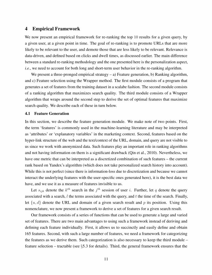
Early search engines provided generic results – for a given query at a given point in time,everyone saw the same results. About a decade back, most major search engines started personalizingresults based on geographic location and language. These strategies can be interpreted as segment-based personalization, since they assume that consumers sharing similar geographies or languagesalso share similar tastes. More recently, search engines have started personalizing based onindividual-level data on past browsing behavior. In December 2009, Google launched personalizedsearch, which customizes results based on a user’s IP address and cookie, using up to 180 days ofhistory, even when a user is not signed into Google (Google Official Blog, 2009). Since then, othersearch engines such as Bing and Yandex have also started personalizing their results (Sullivan, 2011;Yandex, 2013). See Figure 1 for an example of how personalization can influence search results.

Since its adoption, the extent and effectiveness of search personalization has been a source ofintense debate, partly fueled by the secrecy of search engines on how they implement personaliza-tion.2 Google itself argues that information from a user’s previous queries is used in less than 0.3%

of its searches (Schwartz, 2012). However, in a field study with 200 users, Hannak et al. (2013)find that 11.7% of results show differences due to personalization. Interestingly, they attributethese differences to searching with a logged in account and the IP user’s address rather than searchhistory. Thus, the role of search and click history within and across sessions on the extent andeffectiveness of personalization remains unclear. Indeed, some researchers have even questionedthe value of personalizing search results, not only in the context of search engines, but also inthat of hotel industry (Feuz et al., 2011; Ghose et al., 2014). In fact, this debate on the returns tosearch personalization is part of a larger one on the returns to personalization of any marketing mixvariable. (See §2 for details.)

Broadly speaking, there are four main questions of both research and managerial interest thatwe have no clear answers for. First, how effective is search personalization in the field? In principle,

2In Google’s case, the only source of information on its personalization strategy is a post in Google’s official blog,which suggests that whether a user previously clicked a page and the temporal order of a user’s queries influence herpersonalized rankings (Singhal, 2011). In the case of Yandex, all that we know comes from the following quote byone of its executive, Mr.Bakunov – “Our testing and research shows that our users appreciate an appropriate level ofpersonalization and increase their use of Yandex as a result, so it would be fair to say it can only have a positive impacton our users – though we should stress that search quality is a more important metric for us,” (Atkins-Kruger, 2012).

3

if consumers’ tastes show persistence over time, personalization using historic information onusers’ browsing behavior should improve search results. However, we do not know the degree ofpersistence in tastes and extent to which it can improve search experience. Thus, the effectivenessof search personalization is an open question. Second, which features lead to better results frompersonalization? For example, which of these metrics is more effective in improving results – auser’s propensity to click on the first result or her propensity to click on previously clicked results?Feature engineering is an important aspect of any ranking problem, and is therefore treated as asource of competitive advantage and kept under wraps by most search engines (Liu, 2011). However,all firms that use search would benefit from understanding the relative usefulness of different typesof features; e.g., online retail stores (Amazon, Macy’s), entertainment sites (Netflix, Hulu), andonline app stores (Apple, Google). Third, what is the relative value of within and across sessionpersonalization? On the one hand, we might expect within session personalization to be moreinformative of consumer’s current quest. On the other hand, across session data can help inferpersistence in consumers’ tastes. For example, some consumers may tend click only on the firstresult, while others may be more click-happy. Note that within session personalization has tohappen in real time; so understanding the relative value of within and across session personalizationcan help us decide the computational load the system can/should handle. Fourth, which rankingalgorithm is the most appropriate for this task, and what speed improvements does it provide?

We address these questions using data from Yandex. Yandex is the fourth largest search enginein the world, with over 60% marketshare in Russia (Clayton, 2013; Pavliva, 2013). It generatedover $320 billion US dollars in quarterly revenues in 2013, with 40% growth compared to 2012

(Yandex, 2013). It also has a significant presence is other eastern European countries such asUkraine and Kazakhstan. Nevertheless, Yandex faces serious competition from Google, and islooking to improve its search quality in order to retain/improve its marketshare. Therefore, it notonly invests in internal R&D, but also engages with the research community to improve its searchalgorithm by sponsoring research competitions (called Yandex Cups) and making anonymizedsearch data available to researchers. In October 2013, Yandex released a large-scale anonymizeddataset for a ‘Yandex Personalized Web Search Challenge’, hosted by Kaggle (Kaggle, 2013). Thedata consists of information on anonymized user identifiers, queries, query terms, URLs, URLdomains and clicks. We use this data to train our empirical framework and answer the questionsoutlined earlier.

We present a machine-learning framework that re-ranks search results based on a user’ssearch/click history so that more relevant results are ranked higher. Our framework employsa three-pronged approach – a) Feature generation, b) NDCG-based LambdaMart algorithm, and c)Feature selection using the Wrapper method. The first module consists of a program that generatesa set of features from the training dataset in a scalabe fashion. The second module consists of

4

the LambdaMart ranking algorithm that maximizes search quality, as measured by NormalizedDiscounted Cumulative Gain (NDCG). The third module consists of a Wrapper algorithm that wrapsaround the LambdaMart step to derive the set of optimal features that maximize search quality.

Our framework offers two key advantages. First, it is scalable to ‘big-data’. This is importantsince search datasets tend to be very large. The Yandex data, which spans one month, consistsof 5.7 million users, 21 million unique queries, 34 million search sessions, and over 64 millionclicks. We show that our feature generation module is easily scalable and is critical for the quality ofsearch results. Since some parts of the feature generation algorithm have to be run in real time (e.g.,within-session features), its speed and scalability are key to the overall performance of the method.We also show that the returns to scaling the LambdaMart routine and the Wrapper algorithm arelow after a certain point , which is reassuring since we also find that these are not easily scalable.Thus, in our framework the feature generation module is executed on the entire dataset, whereas theLamdaMart and Wrapper algorithms are run on a subset of the data. We find that this offers thebest results in terms of both speed and performance. Second, our framework can work with fullyanonymized data. In general, anonymization results in the loss of the context of query terms, URLs,and domains, loss of text data in webpages and the hyperlink-structure between them – factorswhich have been shown to play a big role in improving search quality (Qin et al., 2010). Thus,the challenge lies in coming up with a re-ranking algorithm that does not rely on contextual, text,or hyperlink data. Our framework only requires an existing ranking based on such anonymizedvariables and the personal search history for a user. As concerns about user privacy increase, this isan important advantage.

We apply our framework to the Yandex dataset, and present two key results. First, we showthat personalization leads to a 4% increase in search quality (as measured by NDCG), a significantimprovement in this context. This is in contrast to the standard logit-style models. Second, we findthat both types of personalization are valuable – short-term or “within-session” personalization, aswell as long-term or “across-session” personalization.

Our paper makes three main contributions to marketing literature on personalization. First, itpresents an empirical framework that marketers can use to rank recommendations using personalizeddata. Second, it presents empirical evidence in support of the returns to personalization in theonline search context. Third, it demonstrates how large datasets or big-data can be leveraged toimprove marketing outcomes without compromising the speed or real-time performance of digitalapplications.

2 Related LiteratureOur paper relates to many streams of literature in marketing, computer science, and economics.

First, it relates to the theoretical literature on price personalization in marketing and economics.

5

Early research in this area found that price discrimination in static symmetric duopolies can dampenprofits (Shaffer and Zhang, 1995; Bester and Petrakis, 1996; Fudenberg and Tirole, 2000), especiallyif firms cannot perfectly predict consumers’ preferences (Chen et al., 2001). More recently however,Shaffer and Zhang (2000, 2002); Villas-Boas (2006); Chen and Zhang (2009) find that personalizedprices can improve profits if we allow for strategic consumers and inter-temporal substitution.Another dimension in personalized pricing is haggling. Desai and Purohit (2004) show that firmsmay find it profitable to allow consumers to haggle if they face heterogenous haggling costs.Analytical results are mixed in the context of product personalization too. Dewan et al. (1999) findthat firms are more likely to personalize if it is cheap to so and if they can second-degree pricediscriminate. On the other hand, Chen and Iyer (2002) show that firms’ incentives to personalizeis high if consumers’ tastes are heterogenous and cost of personalization is high. While theseanalytical models give valuable insights into the trade-offs involved in personalization, their bare-bones framework cannot inform the empirical effectiveness and costs of personalization, especiallyin search settings, where marketing-mix variables like price don’t play any role.

Second, our paper relates to the empirical literature on personalization in marketing.3 In aninfluential paper, Rossi et al. (1996) quantify the benefits of one-to-one pricing using data onpurchase history and find that personalization improves profits by 7.6%. Similarly, Ansari andMela (2003) find that content-targeted emails can potentially increase the click-throughs up to62%, and Arora and Henderson (2007) find that customized promotions in the form of ‘embeddedpremiums’ or social causes associated with the product can improve profits. On the other hand, aseries of recent papers question the returns to personalization in a variety of contexts ranging fromadvertising to ranking of hotels in travel sites (Zhang and Wedel, 2009; Goldfarb and Tucker, 2011;Lambrecht and Tucker, 2013; Ghose et al., 2014). Substantively, our paper speaks to this ongoingdebate by providing empirical support to the idea that there are indeed returns to personalization,especially in rankings of online search engines. However, it differs from the aforementioned paperson two dimensions. First, they focus on the personalization of marketing mix variables such asprice and advertising, while we focus on product personalization (search engine results). Evenpapers that consider ranking outcomes, e.g., Ghose et al. (2014), use marketing mix variables suchas advertising and pricing to make ranking recommendations. However, in the information retrievalcontext, there are no such marketing-mix variables. Moreover with our anonymized data, wedon’t even have access to the topic/context of search. Second, from a methodological perspective,previous papers use computationally intensive Bayesian methods that employ Markov Chain MonteCarlo (MCMC) procedures, or randomized experiments, or discrete choice models – all of whichare not only difficult to scale, but also lack predictive power (Ansari et al., 2000; Rossi and Allenby,

3This is distinct from the literature on recommendation systems. See Ansari and Jedidi (2000), Chung et al. (2009) inmarketing and Pazzani and Billsus (2007), Jannach et al. (2010) in computer science for discussions on such systems.

6

2003; Friedman et al., 2000). In contrast, we use machine learning methods that can handle big dataand offer high predictive performance.

In a similar vein, our paper also relates to the computer science literature on personalizationof search engine rankings. Qiu and Cho (2006) infer user interests from browsing history usingexperimental data on ten subjects. Teevan et al. (2008) and Eickhoff et al. (2013) show that therecould be returns to personalization for some specific types of searches involving ambiguous queriesand atypical search sessions. Bennett et al. (2012) find that long-term history is useful early in thesession whereas short-term history later in the session. There are two main differences betweenthese papers and ours. First, in all these papers, the researchers had access to the data with ‘context’– information on the URLs and domains of the webpages, the hyperlink structure between them,and the queries used in the search process. In contrast, we work with anonymized data – we don’thave data on the URL identifiers, texts, or links to/from webpages; nor do we know the queries.We simply work with anonymized numerical values for queries, which makes the task significantlymore challenging. We show that personalization is not only feasible, but also beneficial in suchcases. Second, the pervious papers work with much smaller datasets, which helps them avoid thescalability issues that we face.

More broadly, our paper contributes to the growing literature on machine learning methodologiesfor Learning-to-Rank (LETOR) methods. Many information retrieval problems in business contextsoften boil down to ranking. Hence ranking methods have been studies in many different contextssuch as collaborative filtering (Harrington, 2003), question answering (Surdeanu et al., 2008;Banerjee et al., 2009), text mining (Metzler and Kanungo, 2008), and digital advertising (Ciaramitaet al., 2008). We refer interested readers to Liu (2011) for details.

3 Data

3.1 Data Description

We use the publicly available anonymized dataset released by Yandex for its personalizationchallenge (Kaggle, 2013). The dataset is from 2011 (exact dates are not disclosed) and represents27 days of search activity. The queries and users are sampled from a large city in eastern Europe.The data is processed such that two types of sessions are removed – those containing queries withcommercial intent (as detected by Yandex’s proprietary classifier) and those containing one or moreof the top-K most popular queries (where K is not disclosed). This minimizes risks of reverseengineering of users’ identities and business interests.

The data contains information on the following anonymized variables:

• User: A user, indexed by i, is an agent who uses the search engine for information retrieval.Users are tracked over time through a combination of cookies, IP addresses, and logged inaccounts. There are 5, 736, 333 unique users in the data.

7

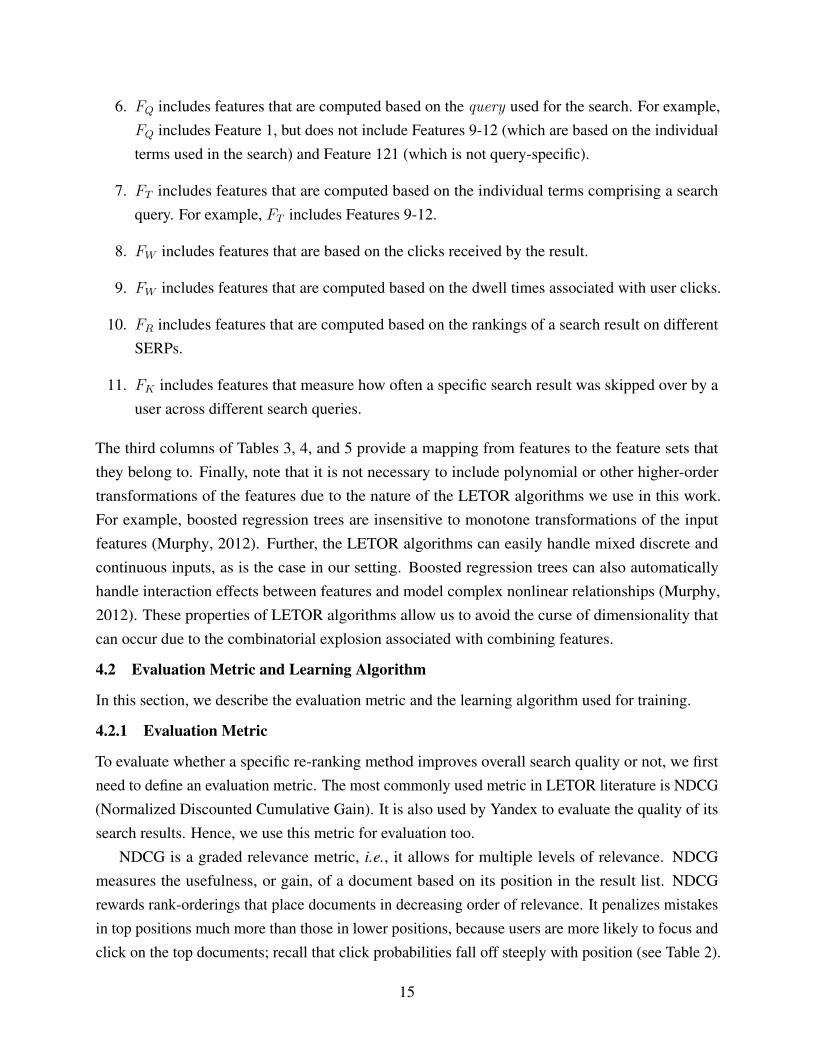
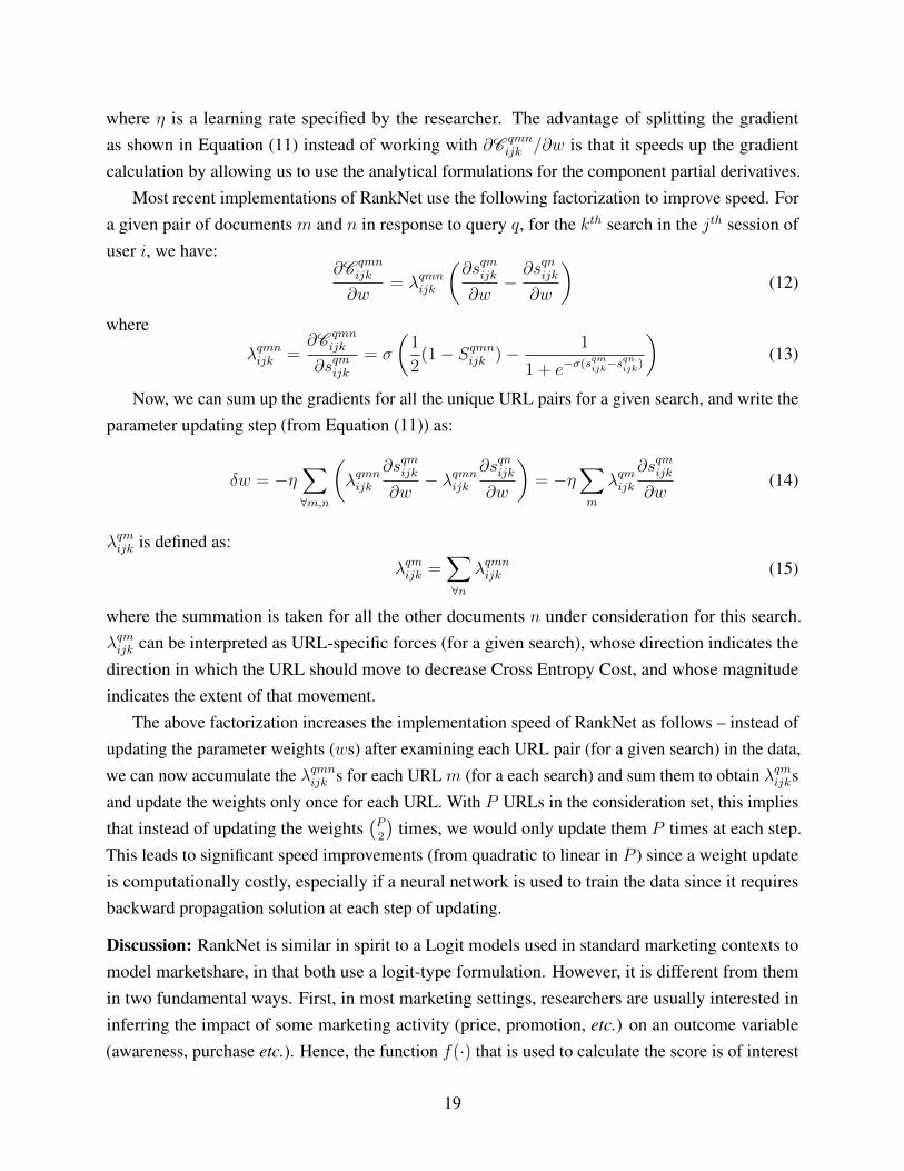
• Query: A query is composed of one or more words, in response to which the search enginereturns a page of results. There are a total of 21, 073, 569 queries in the data.4 Figure 2shows the distribution of queries in the data, which follows a long-tail pattern – 1% of queriesaccount for 47% of the searches, and 5% for 60%.

• Term: Each query consists of one or more terms, and terms are indexed by l. For example,the query ‘pictures of richard armitage’ has three terms – ‘pictures’, ‘richard’, and ‘armitage’.There are 197, 729, 360 unique terms in the data, and we present the distribution of the numberof terms in all the queries seen in the data in Table 1.5

• Session: A search session, indexed by j, is a continuous block of time during which a user isrepeatedly issuing queries, browsing and clicking on results to obtain information on a topic.Search engines use proprietary algorithms to detect session boundaries (Goker and He, 2000);and the exact method used by Yandex is not publicly revealed. According to Yandex, there are34, 573, 630 sessions in the data, and the distribution of sessions per user is shown in Figure 3.Most users, ≈ 40%, participate in only one search session. This does not necessarily indicatehigh user churn because a user may delete cookies, or return from a different device or IPaddress. Nevertheless, a significant number of users can be tracked over time, and the medianuser participates in two sessions, with the mean being 6.1 sessions per users.

• URL: After a user issues a query, the search engine returns a set of ten results in the first page.These results are essentially URLs of webpages relevant to the query. There are 703, 484, 26

unique URLs in the data URLs, and URLs are indexed by u. Yandex only provides data forthe first Search Engine Results Page (SERP) for a given query because a majority of usersnever go beyond the first page, and click data for subsequent pages is very sparse. So from animplementation perspective, it is difficult to personalize later SERPs; and from a managerialperspective, the returns to personalizing them is low since most users never see them.

• URL domain: Is the domain to which a given URL belongs. For example, www.imdb.comis a domain, while http://www.imdb.com/name/nm0035514/ and http://www.imdb.com/name/nm0185819/ are URLs or webpages hosted at this domain.

• Click: After issuing a query, users can click on one or all the results on the SERP. Clickinga URL is an indication of user interest. We observe 64, 693, 054 clicks in the data. So, onaverage, a user clicks on 3.257 results following a query. Table 2 shows the probability of

4Queries are not the same as keywords, which is another term used frequently in connection with search engines. Pleasesee Gabbert (2011) for a simple explanation of the difference between the two phrases.

5Search engines typically ignore common keywords and prepositions used in searches such as ‘of’, ‘a’, ‘in’, becausethey tend to be uninformative. Such words are called ‘Stop Words’.

8

click by position or rank of the result. Note the steep drop off in click probability with position– the first document is gets clicked 44.51% of times, whereas the the fifth one is clicked amere 5.56% of times.

• Time: Yandex gives information on the timeline of each session. However, to preserveanonymity, it does not disclose how many milliseconds are in one unit of time. Each actionin a session comes with a time stamp that tells us how long into the session the action tookplace. Using these time stamps, Yandex calculates ‘dwell time’ for each click, which is thetime between a click and the next click or the next query. Dwell time is informative of howmuch time a user spent with a document.

• Relevance: A result is relevant to a user if she finds it useful, and irrelevant otherwise. Searchengines attribute relevance scores to search results based on user behavior – clicks and dwelltime. It is well known that dwell time is correlated with the probability that the user to satisfiedher information needs with the clicked document. The labeling is done automatically, hence,different for each query issued by the user. Yandex uses three grades of relevance:

• Irrelevant, r = 0.A result gets a irrelevant grade if it doesn’t get a click or if it receives a click with dwelltime strictly less than 50 units of time.

• Relevant, r = 1.Results with dwell times between 50 and 399 time units receive a relevant grade.

• Highly relevant, r = 2.Is given to two types of documents – a) those that received clicks with a dwell time of 400

units or more, and b) if the document was clicked, and the click was the last action of thesession (irrespective of dwell time). The last click of a session is considered to be highlyrelevant because a user is unlikely to have terminated her search if she is not satisfied.

In cases where a document is clicked multiple times after a query, the maximum dwell time isused to calculate the document’s relevance.

In sum, we have a total of 167, 413, 039 lines of data.

3.2 Model-Free Analysis

We now present some model-free evidence that supports the presence of persistence in users’ tastes,and positive returns to personalization. For personalization to be effective, we need to observe twotypes of patterns in the data. First, there has to significant heterogeneity in users’ tastes. Second,users’ tastes have to exhibit persistence over time. Below, we examine the extent to which searchand click patterns support these two hypotheses.

9

First, we need data on user history to model personalization. So we start by examining userhistory metrics. Figure 4 presents the Cumulative Distribution Function (CDF) of the number ofqueries issued by a user. 20% of users issue only one query, making any personalization impossiblefor them. However, 50% of users issue 4 or more queries, with the median queries per user being 4.Further, if we examine the number of queries per session (see Figure 5), we find that 60% of thesessions have only one query. This implies that within session personalization is not possible forsuch sessions. However, 20% of sessions have two or more queries, making them amenable to withinsession personalization. Next, consider the feasibility of across-session personalization. Close to40% of users participate in only one session (Figure 3). While across-session personalization isnot possible for these users, we do observe a significant number of repeat-session users – 40% ofusers participate in 4 or more sessions and 20% in 8 or more. Together, these patterns suggest that areasonable degree of both short and long-term personalization is feasible in this context.

Figure 6 presents the distribution of the average number of clicks per query for the users in thedata. As we can see, there is considerable heterogeneity in users’ propensity to click. For example,more 15% of users don’t click at all, whereas 20% of them click on 1.5 results or more for eachquery they issue. To ensure that these patterns are not driven by one-time or infrequent users, wepresent the same analysis for users who have issued at least 10 queries in Figure 7, which showssimilar click patterns. Together, these two figures establish the presence of significant user-specificheterogeneity in taste for clicking.

Next, we examine whether there is variation or entropy in the URLs that are clicked for a givenquery. Figure 8 presents the cumulative distribution of the number of unique URLs clicked fora given query through the time period of the data. 37% of queries receive no clicks at all, andclose to another 37% receive a click to only one unique URL. These are likely to be navigationalqueries; e.g., almost everyone who searches for ‘cnn’ will click on www.cnn.com. However,close to 30% of queries receive clicks on two or more URLs. This suggests that users are clickingon multiple results. This could be either due to heterogeneity in users’ preferences for differentresults or because there is significant churn in the results for the query (a possibility for news relatedqueries, such as ‘earthquake’). To examine if the last explanation drives all the variation in Figure 8,we plot how many unique URLs and domains we see for a given query through the course of thedata in Figure 9. We find that more than 90% of queries have no churn in the URLs shown in resultspage. Hence, it is unlikely that the entropy in clicked URLs is driven by churn in search engineresults. Rather, it is more likely to be driven in heterogeneity in users’ tastes.

In sum, the basic patterns in the data point to significant heterogeneity users’ preferences andpersistence of those preferences.

10

4 Empirical FrameworkWe now present an empirical framework for re-ranking the top 10 results for a given query, bya given user, at a given point in time. The goal of re-ranking is to promote URLs that are morelikely to be relevant to the user, and demote those that are less likely to be relevant. Relevance isdata-driven, and defined based on clicks and dwell times, as discussed earlier. The main differencebetween a standard re-ranking methodology and the one presented here is the personalization aspect,i.e., we need to account for both long and short-term user behavior in the re-ranking algorithm.

We present a three-pronged empirical strategy – a) Feature generation, b) Ranking algorithm,and c) Feature selection using the Wrapper method. The first module consists of a program thatgenerates a set of features from the training dataset in a scalabe fashion. The second module consistsof a ranking algorithm that maximizes search quality. The third module consists of a Wrapperalgorithm that wraps around the second step to derive the set of optimal features that maximizesearch quality. We describe each of these in turn below.

4.1 Feature Generation

In this section, we describe the feature generation module. We make note of two points. First,the term ‘features’ is commonly used in the machine-learning literature and may be interpretedas ‘attributes’ or ‘explanatory variables’ in the marketing context. Second, features based on thehyper-link structure of the web and the text/context of the URL, domain, and query are not visible tous since we work with anonymized data. Such features play an important role in ranking algorithmsand not having information on them is a significant drawback (Qin et al., 2010). Nevertheless, wehave one metric that can be interpreted as a discretized combination of such features – the currentrank based on Yandex’s algorithm (which does not take personalized search history into account).While this is not perfect (since there is information-loss due to discretization and because we cannotinteract the underlying features with the user-specific ones generated here), it is the best data wehave, and we use it as a measure of features invisible to us.

Let sijk denote the kth search in the jth session of user i. Further, let q denote the queryassociated with a search, l the terms associated with the query, and t the time of the search. Finally,let {u, d} denote the URL and domain of a given search result and p its position. Using thisnomenclature, we now present a framework to derive a set of features for a given search result.

Our framework consists of a series of functions that can be used to generate a large and variedset of features. There are two main advantages to using such a framework instead of deriving anddefining each feature individually. First, it allows us to succinctly and easily define and obtain165 features. Second, with such a large number of features, we need a framework for categorizingthe features as we derive them. Such categorization is also necessary to keep the third module –feature selection – tractable (see §5.3 for details). Third, the general framework ensures that the

11

methods presented in this paper can be extrapolated to other personalized ranking contexts, e.g.,online retailers or entertainment sites.

4.1.1 Functions for Feature Generation

We start with the following support functions that are used to compute four sets of features thatcapture attributes associated with the past history of both the search result and the user.

1. Listings(query , url , usr i, sessionj, time): This function calculates the number of times a urlappeared in a SERP for searches issued by usr i for a given query in the a given session skand before time time.

This function can also be invoked with certain input values left unspecified, in which caseit is computed over all possible values of the unspecified input values. For example, if theuser and session inputs are not provided, then this function is computed over all users acrossall sessions and queries. That is, Listings(query , url ,−,−, time) computes the number ofoccurrences of the url in any SERP associated with the query issued before time t. Further,if t is left unspecified, then the function is computed over the entire dataset excluding thespecific query for which we are computing the features. Another example of a generalizationof the function is obtained by not providing an input value for the query term (as in List-

ings(−, url ,−,−, time)), in which case the count is performed over all SERPs associatedwith all queries; that is, we count the number of times a given url appears in all SERPs seenin the data before a given point in time irrespective of the query.

We also define the following two variants of this function.

• If we supply a search term (term l) as an input instead of a query, then the invocationListings(term l, url , usr i, sessionj, time) takes into account all queries that includeterm l as one of the search terms.

• If we supply a URL domain as an input instead of a URL, then the invocation List-

ings(query , domain, usr i, sessionj, time) will count the number of times that a resultfrom domain appeared in the SERP in the searches associated with a given query .

2. Clicks(query , url , usr i, sessionj, time): This function calculates the number of times thatusr i clicked on a given url after seeing it on a SERP provided in response to searches forquery within sessionj and before time. Clicks(·) can then be used to compute the click-through rates (CTRs) as follows:

CTR(query , url , usr i, sessionj, time) =Clicks(query , url , usr i, sessionj, time)

Listings(query , url , usr i, sessionj, time)(1)

12

3. Dwells(query , url , usr i, sessionj, time): This function calculates the total amount of timethat usr j dwells on a url after clicking on it in response to a query within a given sessionj

and before time. Dwells can be used to compute the average dwell time (ADT), which is amore informative metric of relevance of a url over and above the click-through rate.

ADT(query , url , usr i, sessionj, time) =Dwells(query , url , usr j, sessionj, time)

Clicks(query , url , usr i, sessionj, time)(2)

4. AvgListRank(query , url , usr i, sessionj, time): This function calculates the average rank of aurl within SERPs that list it in response to searches using a given query within sessionj andbefore time. This function provides information over and above the Listings function as itcharacterizes the average ranking of the result as opposed to simply noting its presence in theSERP. We abbreviate AvgListRank to ALR for the remainder of this paper.

As in the case of Listings, all the above functions can be invoked in their generalized forms withouta specifying a query, user, or session, Similarly, they can also be invoked for terms and domains.The first two columns of Tables 3 and 4 list the features that can be computed using the supportfunctions described above. Note that we use only the first four terms for features computed usingsearch terms (e.g., those numbered 9 through 12). Given that 80% of the queries have four or fewersearch terms (see Table 1), the information loss from doing so is minimal while keeping the numberof features reasonable.

In addition to the above, we also use the following functions to generate additional features.

• ClickProb(usr i, posnp, time). This is the probability that usr i clicks on a search result thatappears at position m within a SERP at time. This function captures the heterogeneity inusers’ preferences for clicking on results appearing at different positions.

• NumSearchResults(query) is the total number of search results appearing on any SERPassociated with query . It is an entropy metric on the extent to which search results associatedwith a query vary over time. This number is likely to be high for news-related queries.

• NumClickedURLs(query) is the total number of unique URLs clicked on any SERP associatedwith that query . It is a measure of the heterogeneity in users’ tastes for information/resultswithin a query. For instance, for navigational queries this number is likely to be very low,whereas for other queries like ‘Egypt’, it is likely to be high since some users may be seekinginformation on the recent political conflict in Egypt, others on tourism to Egypt, while yetothers on the history/culture of Egypt.

• Skips(url , usr i, sessionj, time) is the number of times that user i is presented with a SERPcontaining a specific url in sessionj but chooses to skip over the result and click on a search

13

result that appears below that url in the SERP. This function captures the user’s indifferencefor the search result, and it is more informative than just counting the number of times theresult wasn’t clicked.

• SERPRank(url , usr i, sessionj, searchk). Finally, as mentioned earlier, we include the posi-tion/rank of a result for a given instance of search (kth search in session j for user i) withinthe SERP as a feature. This is informative of many aspects of the query, page, and contextwhich are not visible to us. By using SERPRank(·) as one of the features, we are able to foldin this information into a personalized ranking algorithm.

As before, some of these functions can be be invoked more generally, and the list of featuresgenerated through them are listed in Table 5).

4.1.2 Categorization of Feature Set

The total number of features that can we can generate from the functions described in the previoustwo sub-sections is very large (165 to be specific). To aid exposition and experiment with the impactof including or excluding certain sets of features in the learning algorithm, we group the above setof features into the following (partially overlapping) categories. This grouping is also provides amore general framework that can be used in other contexts.

1. FP includes all user- or person-specific features except ones that are at session-level granular-ity. For example, FP includes Feature 41, which counts the number of times a specific url

appeared in a SERP for searches issued by usr i for a specific query .

2. FS includes all user-specific features at a session-level granularity. For example, FS includesFeature 81, which measures the number of times a url appeared in a SERP for searches issuedby usr i for a given query in a sessionj .

3. FG includes features that provide global or system-wide statistics regarding searches (i.e.,features which are not user-specific). For example, FG includes Feature 1, which measuresthe number of times url appeared in a SERP for searches involving query irrespective of theuser issuing the search.

4. FU includes features associated with a URL url . For example, FU includes Features 1, 41,81, but not Feature 5, which is a function of the domain name associated with a search result,but not URL.

5. FD includes features that are attributes associate with a domain name dom i that is associatedwith a search result. This set includes features such as Feature 5, which measures the numberof times dom i is the domain name of a result in a SERP provided for query .

14

6. FQ includes features that are computed based on the query used for the search. For example,FQ includes Feature 1, but does not include Features 9-12 (which are based on the individualterms used in the search) and Feature 121 (which is not query-specific).

7. FT includes features that are computed based on the individual terms comprising a searchquery. For example, FT includes Features 9-12.

8. FW includes features that are based on the clicks received by the result.

9. FW includes features that are computed based on the dwell times associated with user clicks.

10. FR includes features that are computed based on the rankings of a search result on differentSERPs.

11. FK includes features that measure how often a specific search result was skipped over by auser across different search queries.

The third columns of Tables 3, 4, and 5 provide a mapping from features to the feature sets thatthey belong to. Finally, note that it is not necessary to include polynomial or other higher-ordertransformations of the features due to the nature of the LETOR algorithms we use in this work.For example, boosted regression trees are insensitive to monotone transformations of the inputfeatures (Murphy, 2012). Further, the LETOR algorithms can easily handle mixed discrete andcontinuous inputs, as is the case in our setting. Boosted regression trees can also automaticallyhandle interaction effects between features and model complex nonlinear relationships (Murphy,2012). These properties of LETOR algorithms allow us to avoid the curse of dimensionality thatcan occur due to the combinatorial explosion associated with combining features.

4.2 Evaluation Metric and Learning Algorithm

In this section, we describe the evaluation metric and the learning algorithm used for training.

4.2.1 Evaluation Metric

To evaluate whether a specific re-ranking method improves overall search quality or not, we firstneed to define an evaluation metric. The most commonly used metric in LETOR literature is NDCG(Normalized Discounted Cumulative Gain). It is also used by Yandex to evaluate the quality of itssearch results. Hence, we use this metric for evaluation too.

NDCG is a graded relevance metric, i.e., it allows for multiple levels of relevance. NDCGmeasures the usefulness, or gain, of a document based on its position in the result list. NDCGrewards rank-orderings that place documents in decreasing order of relevance. It penalizes mistakesin top positions much more than those in lower positions, because users are more likely to focus andclick on the top documents; recall that click probabilities fall off steeply with position (see Table 2).

15

We start by defining the simpler metric, Discounted Cumulative Gain, DCG (Jarvelin andKekalainen, 2000; Jarvelin and Kekalainen, 2002). For a search k, the DCG at position P is definedas:

DCGkP =P∑p=1

2rp − 1

log2(p+ 1)(3)

where rp is the relevance rating of the document (or URL) in position p. DCG is a search-levelmetric defined for the truncation position P . For example, if we are only concerned about the top10 documents for the kth, then we would work with DCGk10.

A problem with DCG is that the contribution of each query to the overall DCG score of thedata varies. For example, a search that retrieves four ordered documents with relevance scores2, 2, 1, 1, will have higher DCG scores compared to a search that retrieves four ordered documentswith relevance scores 1, 1, 0, 0. This is problematic, especially for re-ranking algorithms, where weonly care about the relative ordering of documents. To address this issue, a normalized version ofDCG is used:

NDCGkP =DCGkP

IDCGkP

(4)

where IDCGkP is the ideal DCG at truncation position P for search k. NDCG always takes valuesfrom between 0 and 1. Since NDCG is computed for each search in the training data and thenaveraged over all queries in the training set, no matter how poorly the documents associated with aparticular query are ranked, it will not dominate the evaluation process since each query contributessimilarly to the average measure.

There are two main advantages of NDCG. First, it allows a researcher to specify the number ofpositions that she is interested in. For example, if we only care about the first page of search results,then we can work with NDCGk10; instead if we are interested in the first two pages, we can workwith NDCGk20. Second, NDCG is a list-level metric; it allows us to evaluate the quality of resultsfor the entire list of results with built-in penalties for mistakes at each position.

Nevertheless, NDCG suffers from a tricky disadvantage. It is based on discrete positions, whichmakes its optimization very difficult. For instance, if we were to use a optimizer that uses continuousscores, then we would find that the relative positions of two documents (based on NDCG) willnot change unless there are significant changes in their rank scores. So we could obtain the samerank orderings for multiple parameter values of the model. This is an important consideration thatconstrains the types of optimization methods that can be used to maximize NDCG.

We now describe three Learning to Rank (LETOR) algorithms, in increasing order of sophis-tication and correctness, that can be used to solve re-ranking problem to improve search quality –RankNet, LambdaRank, and LambdaMART.

16

4.2.2 RankNet – Pairwise learning with gradient descent

In an influential paper, Burges et al. (2005) proposed one of the earliest ranking algorithms –RankNet. Versions of RankNet are used by commercial search engines such as Bing (Liu, 2011).

RankNet is a pairwise learning algorithm, i.e., it employs a loss function defined over a pair ofdocuments. Let xquijk ∈ RF denote a set of F features for document/URL u in response to a query qfor the kth search in the jth session of user i. The function f(·) maps the feature vector to a scoresquijk such that squijk = f(xquijk;w), where w is a set of parameters that define the function f(·). squijkcan be interpreted as the gain or value associated with document u for query q for user i in the kth

search in her jth session. Let U qmijk /U qn

ijk denote the event that URL m should be ranked higherthan n for query q for user i in the kth search of her jth session. For example, if m has been labeledhighly relevant (rm = 2) and n has been labeled irrelevant (rn = 0), then U qm

ijk /U qnijk . Note that

the labels for the same URLs can vary with queries, users, and across and within the session; hencethe super-scripting by q and sub-scripting by i, j, and k.

Given two documents m and n associated with a search, RankNet maps the input feature vectorsof the two documents, {xqmijk, x

qnijk}, to the probability that document m is more relevant than n using

a sigmoid function:

P qmnijk = P (U qm

ijk /U qnijk ) =

1

1 + e−σ(sqmijk−s

qnijk)

(5)

where the choice of the parameter σ determines the shape of the sigmoid. Sigmoid functions arecommonly used in the machine learning literature for classification problems, and are known toperform well (Baum and Wilczek, 1988).

Using these probabilities, we can define the log-Likelihood of observing the data. In the machinelearning literature, this is referred to as Cross Entropy Cost function, which is interpreted as thepenalty imposed for deviations of model predicted probabilities from the desired probabilities.

C qmnijk = −P qmn

ijk log(P qmnijk )− (1− P qmn

ijk ) log(1− P qmnijk ) (6)

C =∑i

∑j

∑k

∑∀m,n

C qmnijk (7)

where P qmnijk is the observed probability (in data) that m is more relevant than n. The summation in

Equation (7) is taken in this order – first, over all pairs of URLs ({m,n}) in the consideration setfor the kth search in session j for user i, next over all the searches within session j, then over all thesessions for the user i. Let Sqijk ∈ {0, 1,−1}, where Sqmnijk = 1 if m is more relevant than n, −1 if nis more relevant than m, and 0 if they are equally relevant. Thus, we have P qmn

ijk = 12(1 + Sqmnijk ),

17

and we can rewrite C qmnijk as:

C qmnijk =

1

2(1− Sqmnijk )σ(sqmijk − s

qnijk) + log(1 + e−σ(s

qmijk−s

qnijk)) (8)

Note that Cross Entropy function is symmetric; it is invariant to swapping m and n and flipping thesign of Sqmnijk .6 Further, we have:

C qmnijk = log(1 + e−σ(s

qmijk−s

qnijk) if Sqmnijk = 1

C qmnijk = log(1 + e−σ(s

qnijk−s

qmijk) if Sqmnijk = −1

C qmnijk =

1

2σ(sqmijk − s

qnijk) + log(1 + e−σ(s

qmijk−s

qnijk)) if Sqmnijk = 0 (9)

If the function f(·) is known or specified by the researcher, minimizing the cost is equivalent to astandard Likelihood maximization, which can be estimated using commonly available optimizationmethods such as Newton-Raphson or BFGS. However, in most most predictive modeling scenarios,the functional form f(·) is not known. Moreover, if maximizing the predictive ability of the modelis the goal (as it is here), manual experimentation to arrive at an optimal functional form is timeconsuming and inefficient, especially one that is sufficiently flexible (non-linear) to capture themyriad interaction patterns in the data. As the number of features available expands, this problembecomes exponentially difficult. In our case, we have 165 features; deriving the optimal non-linearcombination of these features that maximizes the predictive ability of the model by experimentationis not feasible. To address these challenges, researchers and managers have turned to solutions fromthe machine learning literature – neural networks and multiple additive regression trees (MART).These machine learning algorithms not only learn the optimal parameters w, but also learn thefunctional form of f(·). The original implementation of RankNet employed a neural network tolearn the function f(·) and optimize w. However, others have experimented with MART, whichworks well too. Both algorithms require a cost function, and a gradient specification.

The gradient of the Cross Entropy Cost function is:

∂C qmnijk

∂sqmijk= −

∂C qnmijk

∂sqnijk= σ

(1

2(1− Sqmnijk )− 1

1 + e−σ(sqmijk−s

qnijk)

)(10)

We can now employ a stochastic gradient descent algorithm to update the parameters, w, of themodel, as follows:

w → w − η∂C qmn

ijk

∂w= w − η

(∂C qmn

ijk

∂sqmijk

∂sqmijk∂w

+∂C qnm

ijk

∂sqnijk

∂sqnijk∂w

)(11)

6Asymptotically, Cqmnijk becomes linear if the scores give the wrong ranking and zero if they give the correct ranking.

18

where η is a learning rate specified by the researcher. The advantage of splitting the gradientas shown in Equation (11) instead of working with ∂C qmn

ijk /∂w is that it speeds up the gradientcalculation by allowing us to use the analytical formulations for the component partial derivatives.

Most recent implementations of RankNet use the following factorization to improve speed. Fora given pair of documents m and n in response to query q, for the kth search in the jth session ofuser i, we have:

∂C qmnijk

∂w= λqmnijk

(∂sqmijk∂w−∂sqnijk∂w

)(12)

where

λqmnijk =∂C qmn

ijk

∂sqmijk= σ

(1

2(1− Sqmnijk )− 1

1 + e−σ(sqmijk−s

qnijk)

)(13)

Now, we can sum up the gradients for all the unique URL pairs for a given search, and write theparameter updating step (from Equation (11)) as:

δw = −η∑∀m,n

(λqmnijk

∂sqmijk∂w− λqmnijk

∂sqnijk∂w

)= −η

∑m

λqmijk∂sqmijk∂w

(14)

λqmijk is defined as:λqmijk =

∑∀n

λqmnijk (15)

where the summation is taken for all the other documents n under consideration for this search.λqmijk can be interpreted as URL-specific forces (for a given search), whose direction indicates thedirection in which the URL should move to decrease Cross Entropy Cost, and whose magnitudeindicates the extent of that movement.

The above factorization increases the implementation speed of RankNet as follows – instead ofupdating the parameter weights (ws) after examining each URL pair (for a given search) in the data,we can now accumulate the λqmnijk s for each URL m (for a each search) and sum them to obtain λqmijksand update the weights only once for each URL. With P URLs in the consideration set, this impliesthat instead of updating the weights

(P2

)times, we would only update them P times at each step.

This leads to significant speed improvements (from quadratic to linear in P ) since a weight updateis computationally costly, especially if a neural network is used to train the data since it requiresbackward propagation solution at each step of updating.

Discussion: RankNet is similar in spirit to a Logit models used in standard marketing contexts tomodel marketshare, in that both use a logit-type formulation. However, it is different from themin two fundamental ways. First, in most marketing settings, researchers are usually interested ininferring the impact of some marketing activity (price, promotion, etc.) on an outcome variable(awareness, purchase etc.). Hence, the function f(·) that is used to calculate the score is of interest

19

to the researcher, and is usually specified a priori. In contrast, in LETOR settings, the goal is topredict the best rank-ordering that maximizes consumers’ click probability and dwell-time. In suchcases, assuming the functional form f(·) is detrimental to the predictive ability of the model. Hence,both f(·) and w are inferred simultaneously here. Second, in standard marketing models, ws areusually treated as structural parameters that define the utility associated with an option. So theirdirectionality and magnitude are of interest to researchers and managers. However, in this casethere is no structural interpretation of parameters; in fact, with complex trainers such as neural netsand MART, the number of parameters is very large and are not at all interpretable.

RankNet has a number of advantages. It can be used with any underlying model that isdifferentiable in model parameters. It has been shown to be successful in a number of settings.However, it suffers from three significant disadvantages. First, because it is a pairwise metric,in cases where there are multiple levels of relevance, it doesn’t use all the information available.For example, consider two sets of documents {m1, n1} and {m2, n2} with the following relevancevalues – {1, 0} and {2, 0}. In both cases, RankNet only utilizes the information that m should beranked higher than n and not the actual relevance scores, which makes it inefficient. Second, itoptimizes a pairwise loss function, which does not differentiate between mistakes at the top of thelist from those at the bottom. This is problematic if the goal is to optimize the rank-ordering for theentire list, rather than the relative ranking of pairs of URLs. Third, it optimizes the Cross EntropyCost function, and not our true objective function, NDCG. RankNet utilizes gradient descent whichworks well with the Cross Entropy Cost function that is twice differentiable in the parameter vectorw, while NDCG is not. This mismatch between the true objective function and the optimized

objective function implies that RankNet is not the best algorithm to optimize NDCG (or other listlevel position-based evaluation metrics).

4.2.3 LambdaRank and LambdaMART: Optimizing for NDCG

Note that RankNet’s speed and versatility comes from its gradient descent formulation, whichrequires the loss or cost function to be twice differentiable in model parameters. Ideally, we wouldlike to preserve the gradient descent formulation because of its attractive convergence properties.However, we need to find a way to optimize for NDCG within this framework, even though itis a discontinuous optimization metric that does not lend itself easily to gradient descent easily.LambdaRank, proposed by Burges et al. (2006), addresses this challenge.

The key insight of LambdaRank is that we can directly train a model without explicitly specifyinga cost function, as long as we have gradients of the cost and these gradients are consistent with costfunction that we wish to minimize. Recall that the gradient functions, λqmnijk s, in RankNet can beinterpreted as directional forces that pull documents in the direction of increasing relevance. If adocument m is more relevant than n, then m get an upward pull of magnitude |λqmnijk | and n gets a

20

downward pull of the same magnitude.LambdaRank expands this idea of gradients functioning as directional forces by weighing them

with the change in NDCG caused by swapping the positions of m and n, as follows:

λqmnijk =−σ

1 + e−σ(sqmijk−s

qnijk)|∆NDCGqmn

ijk | (16)

Note that NDCGqmnijk = NDCGqmn

ijk = 0 when the m and n have the same relevance; so λqmnijk = 0 inthose cases. (This is the reason why the term σ

2(1− Sqmnijk ) drops out.) Thus, the algorithm does not

spend effort swapping two documents of the same relevance.Given that we want to maximize NDCG, suppose that there exists a utility or gain function

C qmnijk that satisfies the above gradient equation. (We refer to C qmn

ijk as gain function in this contextsince we are looking to maximize NDCG.) Then, we can continue to use gradient descent to updateour parameter vector w as follows:

w → w + η∂C qmn

ijk

∂w(17)

Using Poincare’s Lemma and a series of empirical results, Yue and Burges (2007) and Donmez et al.(2009), have shown that for the gradient functions defined in Equation (16) correspond to a gainfunction that maximizes NDCG. Thus, we can use these gradient formulations, and follow the sameset of steps as we did for RankNet to maximize NDCG.

The original version of LamdaRank was trained using neural networks. To improve its speed andperformance, Wu et al. (2010) proposed a boosted tree version of LambdaRank – LambdaMART,which is faster and more accurate. LambdaMART has been successfully used in many LETORcompetitions, and an entry using LambdaMART won the 2010 Yahoo! Learning To Rank Challenge(Chapelle and Chang, 2011). We refer interested readers to Burges (2010) for a detailed discussionon the implementation and relative merits of these algorithms. We use the RankLib implementationof LambdaMART.

4.3 Feature Selection

Feature selection is the final step in our empirical approach. Here, we select the optimal subsetof features that maximize the predictive accuracy of the learning algorithm. Feature selection is astandard and necessary step in all machine learning settings that involve supervised learning (suchas ours) because of three reasons (Guyon and Elisseeff, 2003). First, it improves the predictionaccuracy by eliminating irrelevant features whose inclusion could result in overfitting. An overfittedmodel is inferior since it is distorted to explain random error or noise in the data as opposed tocapturing just the underlying relationships in the data. Many machine learning algorithms, includingneural networks, decision trees, CART, and even Naive Bayes learners have been shown to have

21

significantly worse accuracy when trained on data with superflous features (Duda and Hart, 1973;Aha et al., 1991; Breiman et al., 1984; Quinlan, 1993). Second, it provides a faster and morecost-effective predictor by eliminating irrelevant features. This is particularly relevant for traininglarge datasets such as ours. Third, it provides more comprehensible models which offer a betterunderstanding of the underlying data generating process.

In principle, feature selection is straightforward since finding the optimal set of features simplyinvolves an exhaustive search of the feature space. However, with a moderately large number offeatures, this is practically impossible. With F features, an exhaustive search requires 2F runs ofthe algorithm on the training dataset, which is exponentially increasing in F . In fact, this problem isknown to be NP-hard (Amaldi and Kann, 1998).

Wrapper Approach: The Wrapper approach to feature selection addresses this problem byusing a greedy algorithm. We describe it briefly here and refer interested readers to Kohavi andJohn (1997) for a detailed review. Wrappers can be categorized into two types – forward selection

and backward elimination. In forward selection, features are progressively added till the predictionaccuracy does not improve any longer. In contrast, backward elimination Wrappers start with all thefeatures and sequentially eliminates the least valuable features. Both these Wrappers are greedy inthe sense that they do not revisit former decisions to include (in forward selection) or exclude (inbackward elimination) features. In our implementation, we employ a forward-selection Wrapper.

To enable a Wrapper algorithm, we also need to specify a selection as well as a stopping rule.We use the robust Best-first selection rule (Ginsberg, 1993), wherein the most promising node isselected at every decision point. For example, in a forward-selection algorithm with 10 features,at the first node, this algorithm considers 10 versions of the model (each with one of the featuresadded) and then picks the feature whose addition offers the highest prediction accuracy. Further, weuse a conservative stopping rule – we stop when none of the remaining features, added sequentially,increase predictive accuracy.7

Wrappers are greedy algorithms, which offers computational advantages. It reduces the numberof runs of the training algorithm from 2F to F (F+1)

2. While this is significantly less than 2F , it is

still prohibitively expensive for large feature sets. For instance, in our case, this would amount to13613 runs of the training algorithm, which is not feasible. Hence, it is common to use a coarse

Wrapper – that is, run it on ‘sets’ of features as opposed to individual features. In our case, weuse domain-specific knowledge to identify related features and perform the search process byadding/removing groups of related features as opposed to individual ones. This allows us to limitthe number of iterations required for the search process and constrains the search space to a much

7This is equivalent to a ‘stale-search of order k’, where k is the number of remaining features at the decision point(instead of a constant) and the margin for improvement is ε = 0, i.e., we only stop if predictive power does not increaseat all or if it decreases.

22

smaller set of feature subsets. We use the feature categories presented in §4.1.2 as the subsets usedfor feature-selection algorithm. In our implementation, we further constrain the Wrapper algorithmbased on additional domain-specific information, which speeds it up further. Please see §5.2 fordetails.

Wrappers offer many advantages. First, they are agnostic to the underlying learning algorithmand the accuracy metric used for evaluating the predictor. This allows us to compare the performanceof different learning algorithms easily. For instance, we can use different learning algorithms (suchas LambdaMART, RankNet) within the same Wrapper. Second, coarse and greedy Wrappers (likethe ones that we use) have been shown to be particularly computationally advantageous and robustagainst overfitting (Reunanen, 2003).

5 ResultsIn this section, we discuss the results from our estimation. We start with a description of the datasetsused in training, validation, and testing. We then outline our feature selection process and derivethe optimal subset of features that optimizes ranking accuracy without overfitting. Then, we derivethe gains from personalization from training on different subsets of test data. Next, we performexperiments that shed light on the relative importance of the various features used in the model. Weconclude the section with an analysis of the scalability of our framework.

5.1 Datasets – Training, Validation, and Testing

Supervised machine-learning algorithms (such as ours) typically require three datasets – training,validation, and testing. Training data is the set of pre-classifed data used for learning or estimatingthe model, and inferring the model parameters. If only one model is used, the the parameterestimates from this model can be tested on a hold-out sample directly. However, in most MLsettings, including ours, multiple versions of the model are considered. To pick the best modelamong these, the validation data is used. Note that this is a more robust and cleaner approach thanpicking the best model based on the training/estimation data (as is common in economics/marketing).This ensures that the model that performs best ‘out-of-sample’ is picked; as with feature selection,this avoids overfitting issues. Finally, the chosen model’s performance is tested on a separatehold-out sample, which is labeled as the test data. The results from the chosen model on the testdata is considered the final predictive accuracy achieved by our framework.

Note that the features described in §4.1.1 can be broadly categorized into two sets – a) globalfeatures, which are common to all the users in the data, and b) user-specific features that are specificto a given user (could either be within or across session features). In real business settings, managerstypically have data on both global and user-level features at any given point in time. If a firm storesdata for 60 days, then the global data at time t is based on a snapshot of all the users observed fromday t to day t − 60. On the other hand, user-level data for a user i at time t is based on her past

23

behavior, going up to day t − 60. Even if i has been in the system for the last 70 days, the firmwould only have access to the past 60 days of data for her. Similarly, is i was first observed on dayt− 30, then only the past 30 days of her history is available at t. Thus, the user-level data goes fromthe point of observation till the first point in time at which the user is observed or the starting pointof the data, whichever is the later.

In our setting, we have a snapshot of 27 days of data from Yandex. We set aside the first 24 daysfor generating global data. For example, we cannot use the first search we observe on day one ofthe data in our analysis because we have no global or user-level characteristics for that user/session.To generate the training data, we use the sessions from the rest of three days (days 25− 27) of thedata. The global features for these sessions are based on ‘all’ the sessions from the previous 24 days.The user-level features for the kth search in the jth session for a user i at time t is based on all theavailable history of that user up till that specific search. To construct the training and validationdatasets, we use 100,000 users each.

In the last three days of data, we see XXX users (state what percent is used for training,validation, and testing).

The test data is constructed similar to the training and validation data. However, this data ismodified a bit more to accommodate the test objectives. Note that testing whether personalization iseffective or not is only possible if there has to be at least one click. So following Yandex, we filterthe test data in two ways. First, for each user in the test period, we only include all her queries fromthe test period with at least one click with a dwell time of 50 units or more (so, that there is at leastone relevant or highly relevant document). Second, if a test query does not have any short-termcontext (it is the first one in the session) and the user is new (has no search sessions in the trainingperiod), then we remove it from the test data, since it has neither short nor long-term context usefulfor personalization.

5.2 Results: Feature Selection

We use a search process that starts with a minimal singleton feature set that comprises of just theSERPRank(·) feature. We refer to this singleton set and its predictive capacity as the Baseline model,whose accuracy we seek to improve using personalized features. We perform a greedy search bywhich we monotonically grow the feature set by iteratively considering different candidate featuresubsets, evaluating the accuracy of the model enhanced with each of the candidate subsets, and thenadding the most promising candidate subset to derive the next version of the feature set.

Figure 10 depicts this exploration process. For example, in the first iteration, we consideradding the most basic features to the model corresponding to the singleton feature model. Weconsider adding user click data at the URL level (FP ∩ FU ∩ FC) and compare the resulting modelimprovement to that obtained by adding global (or non-user-specific) click data at the URL level

24

(FG ∩ FU ∩ FC). We find that the user-specific features improve the accuracy of the model from0.8019 to 0.8119 (according to the NDCG metric), while adding the global features reduces theaccuracy of the model from 0.8019 to 0.8016. We therefore add the user-specific click features toour feature set and consider expanding it with an additional feature subset in the next step of theprocess. The process terminates when we are not able to find any feature subsets that can be addedwithout reducing the accuracy of the model.

We now describe the notation used in the figure and how it relates to the feature categoriespresented earlier. Sessions represents a set of session-level features, but its interpretation could varybased on what is already part of the feature set that we are trying to grow. For example, in step 2 ofthe process where we are trying to add to a feature set comprising of both the baseline and user-specific click data at the URL level, Sessions represents features corresponding to session-specificclick data at the URL level (i.e., FS ∩ FU ∩ FC) and does not include any session-specific click dataat the domain level. However, in step 3 of the process where the feature set now contains featurescorresponding to click data at the domain level (as it was deemed to be the most effective additionin step 2 of the growing process), Sessions represents features corresponding to session-specificclick data at both the URL and domain levels (i.e., FS ∩ FU ∩ FC ∪ FS ∩ FD ∩ FC). The semanticsof each of these feature subsets is thus a function of what is already in the feature set that we aretrying to grow.

The remainder of the notation used in the figure is as follows: Dwells represents features relatedto dwell times, Posns represents features related to ranks of search results, Doms represents featuresrelated to the domain names associated with the search results, Terms represents features relatedto the terms appearing in the search query, and Skips represents features that measure how often asearch result is skipped.

We now draw attention to certain interesting aspects of the feature selection process depictedin the figure. First, the value of a proposed feature set addition changes with different stages ofthe algorithm. Adding the Skips features at level 3 of the growing process (after adding Doms

reduces the accuracy metric from 0.8281 to 0.8276, while adding it at the end of the feature selectionprocess improves the overall accuracy from 0.8326 to 0.8330. This is likely because Skips providesimproved prediction accuracy only when used in conjunction with other features that have alreadybeen added by the tail end of the process (e.g., Sessions, Posns, and Dwells). This illustrates thenon-linear aspect of the LETOR algorithms and its ability to automatically integrate interactioneffects. Second, certain features are never added to the feature set (e.g., Globals and Terms), andthese features are eliminated from the optimal feature set used in training and testing.8 In our setting,this is likely because the features associated with Globals are already reflected in the SERPRank(·)of the result. Search engines are known to track click statistics globally across all users, and

8Tables 3, 4, and 5 indicate which features are included in the final model.

25

they rank the results based on these click statistics in addition to page relevance and importancemetrics. This also implies that all of the gains that we achieve from our LETOR models are dueto personalization and not due to using better features to capture global click metrics. Third, itis possible that a more fine-grained approach might provide improved modeling performance byincluding some of the discarded features individually. Such a step could be used at the end of thecoarse-grained growing process in order to improve the model fit. We leave this enhancement tofuture work.

5.3 Gains from Personalization

We now derive a model using the selected features and test it on the following different datasets, allof which contain sampled search records from the last three days of the search log.

• Test Set 1: This set comprises of uniformly sampled search queries

• Test Set 2: This set comprises of uniformly sampled search queries with at least one relevantclick for the search. This test set thus eliminates searches that resulted in no clicks, whichimplies that the researcher cannot further improve the ranking accuracy of the results containedin the SERP.

• Test Set 3: This set comprises of uniformly sampled search queries with at least one relevantclick for the search and at least one prior click from the user for a previously issued search.This test set thus includes only those searches with some prior history for the user.

• Test Set 4: This set comprises of uniformly sampled search queries with at least one relevantclick for the search and at least five prior clicks from the user for previously issued searches.

Table 6 shows the accuracy achieved by different models on the different datasets. We use Lamb-daMART as the LETOR algorithm for these tests. We compare the Optimal model comprising ofthe features derived from feature selection with the Baseline model comprising of just SERPRank(·)and a model that includes all of the features presented in Tables 3, 4, and 5. The table also providesthe increase in accuracy gain for the Optimal and full models over Baseline.

We observe that the LETOR models improve ranking accuracy over and above the native rankingcomputed by the search engine provider. Recall that the native ranking captures a large range offactors such as relevance of page content and page rank, which are factors that are not available tothe researcher. Further, note that many of the search queries have only zero or one clicked resultsacross all occurrences of the search query, and for these search queries, search personalization isnot going to provide any additional improvements. It is therefore notable that we are able to furtherimprove on the ranking accuracy of the baseline ranking by about 4% using the Optimal model. As

26

pointed out earlier, since the Optimal model does not include global system-wide features, the gainsin accuracy are primarily due to user personalization.

It is also worth noting that the Optimal model improves on the full model by about 0.5%. Thisindicates the presence of significant overfitting in the full model due to the use of redundant orirrelevant features. This improvement in accuracy underscores the importance of performing featureselection in complex models that employ many features.

We now comment on some issues related to training LETOR models. The operation of Lamb-daMART is dependent on a set of parameters that can be tuned. For instance, the researcher hascontrol over the number of regression trees used in the estimation, the number of leaves in a giventree, the type of normalization employed on the features, etc. In order to be robust to the parametersettings, we use two techniques. First, we normalize the features using their zscores so as to makethe feature scales comparable. Second, we use validation datasets in order to avoid overfitting thetraining data especially when we experiment with large and complex models (i.e., increase thenumber of trees or leaves associated with the regression trees). We observed that these techniquessignificantly improve the robustness of the derived models.

5.4 Comparison of Features

We now perform a comparative analysis of the different types of features included in our Optimal

model. In order to perform this analysis, we take the Optimal model and remove features fromdifferent categories and evaluate the loss in NDCG prediction accuracy as a consequence of theremoval. Table 7 provides the results of testing the pruned models on the different test datasets.

We observe that eliminating user-level features while retaining session-level features results ina loss of 2.17%. In contrast, eliminating session-level features while retaining user-level featuresresults in a loss of only 0.31%. This implies that across session features are more valuable thanwithin-session features and that user behavior is stable over longer time periods. We also observethat eliminating domain name based features also results in a significant loss in prediction accuracy.This shows that domain-level click data information on a per-user basis could be a valuable sourceof information to the search engine. This is likely because users might prefer search results fromdomain names that they trust. Search engines can thus track user preferences with respect todomains sourcing search results and use this information to optimize search ranking.

6 ConclusionIn this paper, we study the personalization of ‘online search’ or ‘information retrieval’. Web searchengines are ubiquitous and used by a large number of consumers for a variety of reasons; e.g.,to gather information on a topic from authoritative sources, to remain up-to-date with breakingnews, to aid purchase decisions. Personalization of search results can therefore have significantimplications for consumers, businesses, governments, and for the search engines themselves.

27

We use publicly available anonymized data from the premier eastern European search engine,Yandex, to model and measure the returns to personalization in the search context. We presenta machine learning algorithm that improves search results through automated personalizationusing gradient-based ranking. We personalize results based on both short-term or “within-session”behavior, as well as long-term or “across-session” behavior of the user. We implement our algorithmon data and show that it improves search results signicantly compared to non-personalized results.

28

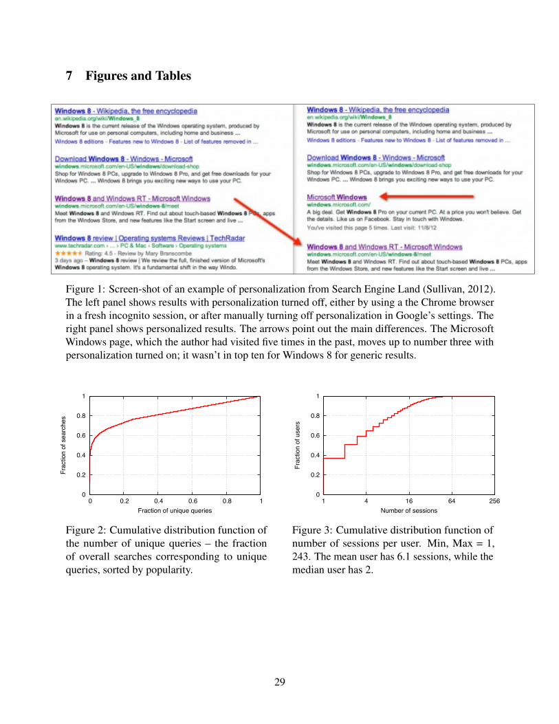
7 Figures and Tables

Figure 1: Screen-shot of an example of personalization from Search Engine Land (Sullivan, 2012).The left panel shows results with personalization turned off, either by using a the Chrome browserin a fresh incognito session, or after manually turning off personalization in Google’s settings. Theright panel shows personalized results. The arrows point out the main differences. The MicrosoftWindows page, which the author had visited five times in the past, moves up to number three withpersonalization turned on; it wasn’t in top ten for Windows 8 for generic results.

0

0.2

0.4

0.6

0.8

1

0 0.2 0.4 0.6 0.8 1

Frac

tion

of s

earc

hes

Fraction of unique queries

Figure 2: Cumulative distribution function ofthe number of unique queries – the fractionof overall searches corresponding to uniquequeries, sorted by popularity.

0

0.2

0.4

0.6

0.8

1

1 4 16 64 256

Frac

tion

of u

sers

Number of sessions

Figure 3: Cumulative distribution function ofnumber of sessions per user. Min, Max = 1,243. The mean user has 6.1 sessions, while themedian user has 2.

29

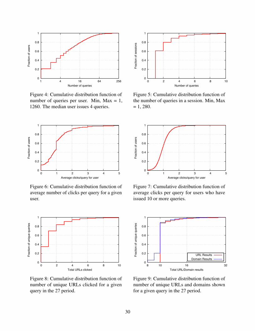
0

0.2

0.4

0.6

0.8

1

1 4 16 64 256

Frac

tion

of u

sers

Number of queries

Figure 4: Cumulative distribution function ofnumber of queries per user. Min, Max = 1,1260. The median user issues 4 queries.

0

0.2

0.4

0.6

0.8

1

0 2 4 6 8 10

Frac

tion

of s

essi

ons

Number of queries

Figure 5: Cumulative distribution function ofthe number of queries in a session. Min, Max= 1, 280.

0

0.2

0.4

0.6

0.8

1

0 1 2 3 4 5

Frac

tion

of u

sers

Average clicks/query for user

Figure 6: Cumulative distribution function ofaverage number of clicks per query for a givenuser.

0

0.2

0.4

0.6

0.8

1

0 1 2 3 4 5

Frac

tion

of u

sers

Average clicks/query for user

Figure 7: Cumulative distribution function ofaverage clicks per query for users who haveissued 10 or more queries.

0

0.2

0.4

0.6

0.8

1

0 2 4 6 8 10

Frac

tion

of u

niqu

e qu

erie

s

Total URLs clicked

Figure 8: Cumulative distribution function ofnumber of unique URLs clicked for a givenquery in the 27 period.

0

0.2

0.4

0.6

0.8

1

8 10 16 32

Frac

tion

of u

niqu

e qu

erie

s

Total URL/Domain results

URL ResultsDomain Results

Figure 9: Cumulative distribution function ofnumber of unique URLs and domains shownfor a given query in the 27 period.

30

Baseline0.8019

+ Users0.8119

+ Globals0.8016

+ Sessions0.8126

+ Dwells0.8119

+ Posns0.8121

+ Doms0.8281

+ Terms0.8129

+ Globals0.8126

+ Skips0.8126

+ Dwells0.8289

+ Posns0.8291

+ Sessions0.8292

+ Terms0.8283

+ Globals0.8259

+ Skips0.8276

+ Dwells0.8294

+ Terms0.8291

+ Posns0.8296

+ Globals0.8278

+ Skips0.8279

+ Terms0.8297

+ Dwells0.8326

+ Globals0.8267

+ Skips0.8295

+ Globals0.8311

+ Skips0.8330

+ Terms0.8279

+ Globals0.8285

+ Terms0.8319

Figure 10: Feature selection process.

31

Number of Terms Percentage ofPer Query Queries

1 22.322 24.853 20.634 14.125 8.186 4.677 2.388 1.279 0.64

10 or more 1.27

Table 1: Distribution of number of terms in a query. The minimum and maximum number of termsin a query are 1 and 82, respectively.

Position Probability of click1 0.44512 0.16593 0.10674 0.07485 0.05566 0.04197 0.03208 0.02589 0.0221

10 0.0206

Table 2: Click probability based on position.

32

Feature No. Feature Name Feature Classes Selected1 Listings(query , url ,−,−,−) FG, FQ, FU , FC

2 CTR(query , url ,−,−,−) FG, FQ, FU , FC

3 ADT(query , url ,−,−,−) FG, FQ, FU , FW

4 ALR(query , url ,−,−,−) FG, FQ, FU , FR

5 Listings(query , domain,−,−,−) FG, FQ, FD, FC

6 CTR(query , domain,−,−,−) FG, FQ, FD, FC

7 ADT(query , domain,−,−,−) FG, FQ, FD, FW

8 ALR(query , domain,−,−,−) FG, FQ, FD, FR

9-12 Listings(term1..4, url ,−,−,−) FG, FT , FU , FC

13-16 CTR(term1..4, url ,−,−,−) FG, FT , FU , FC

17-20 ADT(term1..4, url ,−,−,−) FG, FT , FU , FW

21-24 ALR(term1..4, url ,−,−,−) FG, FT , FU , FR

25-28 Listings(term1..4, domain,−,−,−) FG, FT , FD, FC

29-32 CTR(term1..4, domain,−,−,−) FG, FT , FD, FC

33-36 ADT(term1..4, domain,−,−,−) FG, FT , FD, FW

37-40 ALR(term1..4, domain,−,−,−) FG, FT , FD, FR

41 Listings(query , url , usr i,−, time) FP , FQ, FU , FC X42 CTR(query , url , usr i,−, time) FP , FQ, FU , FC X43 ADT(query , url , usr i,−, time) FP , FQ, FU , FW X44 ALR(query , url , usr i,−, time) FP , FQ, FU , FR X45 Listings(query , domain, usr i,−, time) FP , FQ, FD, FC X46 CTR(query , domain, usr i,−, time) FP , FQ, FD, FC X47 ADT(query , domain, usr i,−, time) FP , FQ, FD, FW X48 ALR(query , domain, usr i,−, time) FP , FQ, FD, FR X

49-52 Listings(term1..4, url , usr i,−, time) FP , FT , FU , FC

53-56 CTR(term1..4, url , usr i,−, time) FP , FT , FU , FC

57-60 ADT(term1..4, url , usr i,−, time) FP , FT , FU , FW

61-64 ALR(term1..4, url , usr i,−, time) FP , FT , FU , FR

65-68 Listings(term1..4, domain, usr i,−, time) FP , FT , FD, FC

69-72 CTR(term1..4, domain, usr i,−, time) FP , FT , FD, FC

73-76 ADT(term1..4, domain, usr i,−, time) FP , FT , FD, FW

77-80 ALR(term1..4, domain, usr i,−, time) FP , FT , FD, FR

81 Listings(query , url , usr i, sessionj , time) FS , FQ, FU , FC X82 CTR(query , url , usr i, sessionj , time) FS , FQ, FU , FC X83 ADT(query , url , usr i, sessionj , time) FS , FQ, FU , FW X84 ALR(query , url , usr i, sessionj , time) FS , FQ, FU , FR X85 Listings(query , domain, usr i, sessionj , time) FS , FQ, FD, FC X86 CTR(query , domain, usr i, sessionj , time) FS , FQ, FD, FC X87 ADT(query , domain, usr i, sessionj , time) FS , FQ, FD, FW X88 ALR(query , domain, usr i, sessionj , time) FS , FQ, FD, FR X

89-92 Listings(term1..4, url , usr i, sessionj , time) FS , FT , FU , FC

93-96 CTR(term1..4, url , usr i, sessionj , time) FS , FT , FU , FC

97-100 ADT(term1..4, url , usr i, sessionj , time) FS , FT , FU , FW

101-104 ALR(term1..4, url , usr i, sessionj , time) FS , FT , FU , FR

105-108 Listings(term1..4, domain, usr i, sessionj , time) FS , FT , FD, FC

109-112 CTR(term1..4, domain, usr i, sessionj , time) FS , FT , FD, FC

113-116 ADT(term1..4, domain, usr i, sessionj , time) FS , FT , FD, FW

117-120 ALR(term1..4, domain, usr i, sessionj , time) FS , FT , FD, FR

Table 3: List of features based on SERPs associated with a given query or terml .

33

Feature No. Feature Name Feature Classes Selected121 Listings(−, url ,−,−,−) FG, FU , FC

122 CTR(−, url ,−,−,−) FG, FU , FC

123 ADT(−, url ,−,−,−) FG, FU , FW

124 ALR(−, url ,−,−,−) FG, FU , FR

125 Listings(−, domain,−,−,−) FG, FD, FC

126 CTR(−, domain,−,−,−) FG, FD, FC

127 ADT(−, domain,−,−,−) FG, FD, FW

128 ALR(−, domain,−,−,−) FG, FD, FR

129 Listings(−, url , usr i,−, time) FP , FU , FC X130 CTR(−, url , usr i,−, time) FP , FU , FC X131 ADT(−, url , usr i,−, time) FP , FU , FW X132 ALR(−, url , usr i,−, time) FP , FU , FR X133 Listings(−, domain, usr i,−, time) FP , FD, FC X134 CTR(−, domain, usr i,−, time) FP , FD, FC X135 ADT(−, domain, usr i,−, time) FP , FD, FW X136 ALR(−, domain, usr i,−, time) FP , FD, FR X137 Listings(−, url , usr i, sessionj , time) FS , FU , FC X138 CTR(−, url , usr i, sessionj , time) FS , FU , FC X139 ADT(−, url , usr i, sessionj , time) FS , FU , FW X140 ALR(−, url , usr i, sessionj , time) FS , FU , FR X141 Listings(−, domain, usr i, sessionj , time) FS , FD, FC X142 CTR(−, domain, usr i, sessionj , time) FS , FD, FC X143 ADT(−, domain, usr i, sessionj , time) FS , FD, FW X144 ALR(−, domain, usr i, sessionj , time) FS , FD, FR X145 Listings(−,−, usr i,−, time) FP , FC X146 CTR(−,−, usr i,−, time) FP , FC X147 ADT(−,−, usr i,−, time) FP , FW X148 Listings(−,−, usr i, sessionj , time) FS , FC X149 CTR(−,−, usr i, sessionj , time) FS , FC X150 ADT(−,−, usr i, sessionj , time) FS , FW X

Table 4: List of features based on all SERPs.

34

Feature No. Feature Name Feature Classes Selected151-160 ClickProb(usr i, posnp, time) FP , FC X

161 NumSearchResults(query) FG, FQ, FC X162 NumClickedURLs(query) FG, FQ, FC X163 Skips(url , usr i,−, time) FP , FU , FK X164 Skips(url , usr i, sessionj , time) FS , FU , FK X165 SERPRank(url , usr i, sessionj , searchk) X

Table 5: Additional Features.

Test Set 1 Test Set 2 Test Set 3 Test Set 4NDCG % Gain NDCG % Gain NDCG % Gain NDCG % Gain

Baseline 0.4655 0.8019 0.8010 0.8013All Features 0.4815 3.32 0.8294 3.32 0.8300 3.49 0.8317 3.65

Optimal 0.4836 3.88 0.8330 3.87 0.8334 4.04 0.8337 4.04

Table 6: Improvements in the NDCG10 metric. We compare the performance of LambdaMARTafter search personalization with: (a) the baseline ranking that is based on the SERP rank providedby the search engine provider, and (b) a ranking model that uses all of the features without employingfeature selection.

Test Set 1 Test Set 2 Test Set 3 Test Set 4NDCG % Loss NDCG % Loss NDCG % Loss NDCG % Loss

Optimal 0.4836 0.8330 0.8334 0.8337− User features 0.4731 2.17 0.8149 2.17 0.8143 2.29 0.8147 2.27− Session features 0.4821 0.31 0.8304 0.31 0.8308 0.31 0.8311 0.31− Dom features 0.4719 2.41 0.8129 2.41 0.8130 2.44 0.8138 2.38− Dwell features 0.4817 0.39 0.8298 0.38 0.8303 0.37 0.8308 0.34− Posn features 0.4824 0.24 0.8309 0.25 0.8313 0.25 0.8317 0.23− Skip features 0.4827 0.18 0.8314 0.19 0.8318 0.19 0.8321 0.19

Table 7: Loss in prediction accuracy when different feature sets are removed from the Optimalmodel.

35

ReferencesD. W. Aha, D. Kibler, and M. K. Albert. Instance-based Learning Algorithms. Machine learning, 6(1):37–66,

1991.E. Amaldi and V. Kann. On the Approximability of Minimizing Nonzero Variables or Unsatisfied Relations

in Linear Systems. Theoretical Computer Science, 209(1):237–260, 1998.A. Ansari and K. Jedidi. Bayesian Factor Analysis for Multilevel Binary Observations. Psychometrika, 65

(4):475–496, 2000.A. Ansari and C. F. Mela. E-customization. Journal of Marketing Research, pages 131–145, 2003.A. Ansari, S. Essegaier, and R. Kohli. Internet Recommendation Systems. Journal of Marketing research, 37

(3):363–375, 2000.N. Arora and T. Henderson. Embedded Premium Promotion: Why it Works and How to Make it More

Effective. Marketing Science, 26(4):514–531, 2007.N. Arora, X. Dreze, A. Ghose, J. D. Hess, R. Iyengar, B. Jing, Y. Joshi, V. Kumar, N. Lurie, S. Neslin, et al.

Putting One-to-One Marketing to Work: Personalization, Customization, and Choice. Marketing Letters,19(3-4):305–321, 2008.

A. Atkins-Kruger. Yandex Launches Personalized Search Results For East-ern Europe, December 2012. URL http://searchengineland.com/yandex-launches-personalized-search-results-for-eastern-europe-142186.

S. Banerjee, S. Chakrabarti, and G. Ramakrishnan. Learning to Rank for Quantity Consensus Queries.In Proceedings of the 32nd international ACM SIGIR Conference on Research and Development inInformation Retrieval, pages 243–250. ACM, 2009.

E. B. Baum and F. Wilczek. Supervised Learning of Probability Distributions by Neural Networks. In NeuralInformation Processing Systems, pages 52–61. New York: AIP, 1988.

P. N. Bennett, R. W. White, W. Chu, S. T. Dumais, P. Bailey, F. Borisyuk, and X. Cui. Modeling the Impactof Short- and Long-term Behavior on Search Personalization. In Proceedings of the 35th InternationalACM SIGIR Conference on Research and Development in Information Retrieval, pages 185–194, 2012.

H. Bester and E. Petrakis. Coupons and Oligopolistic Price Discrimination. International Journal of IndustrialOrganization, 14(2):227–242, 1996.

J. S. Breese, D. Heckerman, and C. Kadie. Empirical Analysis of Predictive Algorithms for CollaborativeFiltering. In Proceedings of the Fourteenth Conference on Uncertainty in Artificial Intelligence, pages43–52. Morgan Kaufmann Publishers Inc., 1998.

L. Breiman, J. Friedman, C. Stone, and R. Olshen. Classification and Regression Trees. The Wadsworth andBrooks-Cole statistics-probability series. Taylor & Francis, 1984.

C. Burges. From RankNet to LambdaRank to LambdaMART: An Overview. Technical report, MicrosoftResearch Technical Report MSR-TR-2010-82, 2010.

C. Burges, T. Shaked, E. Renshaw, A. Lazier, M. Deeds, N. Hamilton, and G. Hullender. Learning to RankUsing Gradient Descent. In Proceedings of the 22nd International Conference on Machine Learning,pages 89–96. ACM, 2005.

C. J. Burges, R. Ragno, and Q. V. Le. Learning to Rank with Nonsmooth Cost Functions. In Advances inNeural Information Processing Systems, pages 193–200, 2006.

O. Chapelle and Y. Chang. Yahoo! Learning to Rank Challenge Overview. Journal of Machine LearningResearch-Proceedings Track, 14:1–24, 2011.

Y. Chen and G. Iyer. Research Note Consumer Addressability and Customized Pricing. Marketing Science,21(2):197–208, 2002.

Y. Chen and Z. J. Zhang. Dynamic Targeted Pricing with Strategic Consumers. International Journal ofIndustrial Organization, 27(1):43–50, 2009.

Y. Chen, C. Narasimhan, and Z. J. Zhang. Individual Marketing with Imperfect Targetability. Marketing

36

Science, 20(1):23–41, 2001.T. S. Chung, R. T. Rust, and M. Wedel. My Mobile Music: An Adaptive Personalization System for Digital

Audio Players. Marketing Science, 28(1):52–68, 2009.M. Ciaramita, V. Murdock, and V. Plachouras. Online Learning from Click Data for Sponsored Search. In

Proceedings of the 17th International Conference on World Wide Web, pages 227–236. ACM, 2008.N. Clayton. Yandex Overtakes Bing as Worlds Fourth Search Engine,

2013. URL http://blogs.wsj.com/tech-europe/2013/02/11/yandex-overtakes-bing-as-worlds-fourth-search-engine/.

comScore. December 2013 U.S. Search Engine Rankings, 2014. URL http://investor.google.com/financial/tables.html.

B. G. Dellaert and S. Stremersch. Marketing Mass-Customized Products: Striking a Balance Between Utilityand Complexity. Journal of Marketing Research, pages 219–227, 2005.

P. S. Desai and D. Purohit. Let me Talk to My Manager: The Costs and Benefits of Haggling. MarketingScience, 23(2):219–233, 2004.

R. Dewan, B. Jing, and A. Seidmann. One-to-One Marketing on the Internet. In Proceedings of the 20thInternational Conference on Information Systems, pages 93–102. Association for Information Systems,1999.

P. Donmez, K. M. Svore, and C. J. Burges. On the Local Optimality of LambdaRank. In Proceedings of the32nd international ACM SIGIR Conference on Research and Development in Information Retrieval, pages460–467. ACM, 2009.

R. O. Duda and P. E. Hart. Pattern Recognition and Scene Analysis, 1973.C. Eickhoff, K. Collins-Thompson, P. N. Bennett, and S. Dumais. Personalizing Atypical Web Search

Sessions. In Proceedings of the Sixth ACM International Conference on Web Search and Data Mining,pages 285–294, 2013.

M. Feuz, M. Fuller, and F. Stalder. Personal Web Searching in the Age of Semantic Capitalism: Diagnosingthe Mechanisms of Personalisation. First Monday, 16(2), 2011.

J. Friedman, T. Hastie, R. Tibshirani, et al. Additive Logistic Regression: A Statistical View of Boosting(with Discussion and a Rejoinder by the Authors). The Annals of Statistics, 28(2):337–407, 2000.

D. Fudenberg and J. Tirole. Customer Poaching and Brand Switching. RAND Journal of Economics, pages634–657, 2000.

E. Gabbert. Keywords vs. Search Queries: What’s the Difference?, 2011. URL http://www.wordstream.com/blog/ws/2011/05/25/keywords-vs-search-queries.

A. Ghose, P. G. Ipeirotis, and B. Li. Examining the Impact of Ranking on Consumer Behavior and SearchEngine Revenue. Management Science, 2014.

M. Ginsberg. Essentials of Artificial Intelligence. Newnes, 1993.A. Goker and D. He. Analysing Web Search Logs to Determine Session Boundaries for User-oriented

Learning. In Adaptive Hypermedia and Adaptive Web-Based Systems, pages 319–322, 2000.A. Goldfarb and C. Tucker. Online display advertising: Targeting and obtrusiveness. Marketing Science, 30

(3):389–404, 2011.Google. How Search Works, 2014. URL http://www.google.com/intl/en_us/insidesearch/howsearchworks/thestory/.

Google Official Blog. Personalized Search for Everyone, 2009. URL http://googleblog.blogspot.com/2009/12/personalized-search-for-everyone.html.

P. Grey. How Many Products Does Amazon Sell?, 2013. URL http://export-x.com/2013/12/15/many-products-amazon-sell/.

I. Guyon and A. Elisseeff. An Introduction to Variable and Feature Selection. The Journal of MachineLearning Research, 3:1157–1182, 2003.

37

A. Hannak, P. Sapiezynski, A. Molavi Kakhki, B. Krishnamurthy, D. Lazer, A. Mislove, and C. Wilson.Measuring Personalization of Web Search. In Proceedings of the 22nd International Conference on WorldWide Web, pages 527–538. International World Wide Web Conferences Steering Committee, 2013.

E. F. Harrington. Online Ranking/Collaborative Filtering using the Perceptron Algorithm. In ICML,volume 20, pages 250–257, 2003.

C. Huffman and B. E. Kahn. Variety for Sale: Mass Customization or Mass Confusion? Journal of Retailing,74(4):491–513, 1998.

InstantWatcher. InstantWatcher.com, 2014. URL http://instantwatcher.com/titles/all.D. Jannach, M. Zanker, A. Felfernig, and G. Friedrich. Recommender Systems: An Introduction. Cambridge

University Press, 2010.K. Jarvelin and J. Kekalainen. IR Evaluation Methods for Retrieving Highly Relevant Documents. In

Proceedings of the 23rd Annual International ACM SIGIR Conference on Research and Development inInformation Retrieval, SIGIR ’00, pages 41–48. ACM, 2000.

K. Jarvelin and J. Kekalainen. Cumulated Gain-based Evaluation of IR Techniques. ACM Transactions onInformation Systems (TOIS), 20(4):422–446, 2002.

Kaggle. Personalized Web Search Challenge, 2013. URL http://www.kaggle.com/c/yandex-personalized-web-search-challenge.

R. Kohavi and G. H. John. Wrappers for Feature Subset Selection. Artificial intelligence, 97(1):273–324,1997.

A. Lambrecht and C. Tucker. When Does Retargeting Work? Information Specificity in Online Advertising.Journal of Marketing Research, 50(5):561–576, 2013.

T. Y. Liu. Learning to Rank for Information Retrieval. Springer, 2011.D. Metzler and T. Kanungo. Machine Learned Sentence Selection Strategies for Query-biased Summarization.

In SIGIR Learning to Rank Workshop, 2008.K. P. Murphy. Machine Learning: A Probabilistic Perspective. The MIT Press, 2012. ISBN 0262018020,

9780262018029.Nielsen. Nielsen Netratings Search Engine Ratings Report, 2003. URL http://searchenginewatch.com/reports/article.php/2156461.

H. Pavliva. Google-Beater Yandex Winning Over Wall Street on AdView, 2013. URL http://www.bloomberg.com/news/2013-04-25/google-tamer-yandex-amasses-buy-ratings-russia-overnight.html.

M. J. Pazzani and D. Billsus. Content-based Recommendation Systems. In The Adaptive Web: Methods andStrategies of Web Personalization. Volume 4321 of Lecture Notes in Computer Science. 2007.

T. Qin, T.-Y. Liu, J. Xu, and H. Li. LETOR: A Benchmark Collection for Research on Learning to Rank forInformation Retrieval. Information Retrieval, 13(4):346–374, 2010.

F. Qiu and J. Cho. Automatic Identification of User Interest for Personalized Search. In Proceedings of the15th International Conference on World Wide Web, pages 727–736, 2006.

J. R. Quinlan. C4. 5: Programs for Machine Learning, volume 1. Morgan kaufmann, 1993.J. Reunanen. Overfitting in Making Comparisons Between Variable Selection Methods. The Journal of

Machine Learning Research, 3:1371–1382, 2003.P. E. Rossi and G. M. Allenby. Bayesian Statistics and Marketing. Marketing Science, 22(3):304–328, 2003.P. E. Rossi, R. E. McCulloch, and G. M. Allenby. The Value of Purchase History Data in Target Marketing.

Marketing Science, 15(4):321–340, 1996.B. Schwartz. Google: Previous Query Used On 0.3% Of Searches, 2012. URL http://www.seroundtable.com/google-previous-search-15924.html.

G. Shaffer and Z. J. Zhang. Competitive Coupon Targeting. Marketing Science, 14(4):395–416, 1995.G. Shaffer and Z. J. Zhang. Pay to Switch or Pay to Stay: Preference-Based Price Discrimination in Markets

38

with Switching Costs. Journal of Economics & Management Strategy, 9(3):397–424, 2000.G. Shaffer and Z. J. Zhang. Competitive One-to-One Promotions. Management Science, 48(9):1143–1160,

2002.D. Silverman. IAB Internet Advertising Revenue Report, October 2013. URL http://www.iab.net/media/file/IABInternetAdvertisingRevenueReportHY2013FINALdoc.pdf.

A. Singhal. Some Thoughts on Personalization, 2011. URL http://insidesearch.blogspot.com/2011/11/some-thoughts-on-personalization.html.

D. Sullivan. Bing Results Get Localized & Personalized, 2011. URL http://searchengineland.com/bing-results-get-localized-personalized-64284.

M. Surdeanu, M. Ciaramita, and H. Zaragoza. Learning to Rank Answers on Large Online QA Collections.In ACL, pages 719–727, 2008.

J. Teevan, S. T. Dumais, and D. J. Liebling. To Personalize or Not to Personalize: Modeling Queries withVariation in User Intent. In Proceedings of the 31st Annual International ACM SIGIR Conference onResearch and Development in Information Retrieval, pages 163–170, 2008.

J. M. Villas-Boas. Dynamic Competition with Experience Goods. Journal of Economics & ManagementStrategy, 15(1):37–66, 2006.

Q. Wu, C. J. Burges, K. M. Svore, and J. Gao. Adapting Boosting for Information Retrieval Measures.Information Retrieval, 13(3):254–270, 2010.

Yandex. It May Get Really Personal We have Rolled Out Our Second–Generation Personalised SearchProgram, 2013. URL http://company.yandex.com/press_center/blog/entry.xml?pid=20.

Yandex. Yandex Announces Third Quarter 2013 Financial Results, 2013. URL http://company.yandex.com/press_center/blog/entry.xml?pid=20.

YouTube. YouTube Statistics, 2014. URL https://www.youtube.com/yt/press/statistics.html.

Y. Yue and C. Burges. On Using Simultaneous Perturbation Stochastic Approximation for IR measures, andthe Empirical Optimality of LambdaRank. In NIPS Machine Learning for Web Search Workshop, 2007.

J. Zhang and M. Wedel. The Effectiveness of Customized Promotions in Online and Offline Stores. Journalof Marketing Research, 46(2):190–206, 2009.

39