on June 19, 2018 Guidedwaves’dispersion rspa...

rspa.royalsocietypublishing.org

ResearchCite this article: Hernando Quintanilla F, FanZ, Lowe MJS, Craster RV. 2015 Guided waves’dispersion curves in anisotropic viscoelasticsingle- and multi-layered media. Proc. R.Soc. A 471: 20150268.http://dx.doi.org/10.1098/rspa.2015.0268

Received: 22 April 2015Accepted: 22 September 2015

Subject Areas:mechanical engineering,computational mathematics, wave motion

Keywords:guided waves, viscoelasticity, generalanisotropy, spectral collocation methods,dispersion curves, non-destructive evaluation

Author for correspondence:F. Hernando Quintanillae-mail: [email protected]

Guided waves’ dispersioncurves in anisotropicviscoelastic single- andmulti-layered mediaF. Hernando Quintanilla1, Z. Fan3, M. J. S. Lowe1

and R. V. Craster2

1Department of Mechanical Engineering, and 2Department ofMathematics, Imperial College London , London SW7 2AZ, UK3School of Mechanical and Aerospace Engineering, NanyangTechnological University, 50 Nanyang Avenue, Singapore 639798,Republic of Singapore

Guided waves propagating in lossy media areencountered in many problems across different areasof physics such as electromagnetism, elasticity andsolid-state physics. They also constitute essential toolsin several branches of engineering, aerospace andaircraft engineering, and structural health monitoringfor instance. Waveguides also play a central rolein many non-destructive evaluation applications. Itis of paramount importance to accurately representthe material of the waveguide to obtain reliableand robust information about the guided wavesthat might be excited in the structure. A reasonableapproximation to real solids is the perfectly elasticapproach where the frictional losses within the solidare ignored. However, a more realistic approachis to represent the solid as a viscoelastic mediumwith attenuation for which the dispersion curvesof the modes are, in general, different from theirelastic counterparts. Existing methods are capable ofcalculating dispersion curves for attenuated modesbut they can be troublesome to find and the solutionsare not as reliable as in the perfectly elastic case. Inthis paper, in order to achieve robust and accurateresults for viscoelasticity a spectral collocation methodis developed to compute the dispersion curves ingenerally anisotropic viscoelastic media in flat andcylindrical geometry. Two of the most popular modelsto account for material damping, Kelvin–Voigt andHysteretic, are used in various cases of interest.

2015 The Author(s) Published by the Royal Society. All rights reserved.

on July 15, 2018http://rspa.royalsocietypublishing.org/Downloaded from

http://crossmark.crossref.org/dialog/?doi=10.1098/rspa.2015.0268&domain=pdf&date_stamp=2015-10-28

mailto:francisco.hernando-quintanilla11@\penalty -\@M imperial.ac.uk

http://rspa.royalsocietypublishing.org/

2

rspa.royalsocietypublishing.orgProc.R.Soc.A471:20150268

...................................................

These include orthorhombic and triclinic materials in single- or multi-layered arrays. Also,and due to its importance in industry, a section is devoted to pipes filled with viscousfluids. The results are validated by comparison with those from semi-analytical finite-elementsimulations.

1. IntroductionRobust and reliable computation of dispersion curves is key for the successful development ofnon-destructive evaluation (NDE) techniques using guided waves. Dispersion curves providethe information required to correctly select propagating modes for the study of the NDE of aparticular type of defect, or some property of the materials, in a structure. The usage of dispersioncurves for NDE is well established as the copious literature and studies on the subject show:analytical solutions using potentials or the partial wave decomposition for the isotropic plate andcylinder were found by Mindlin [1], Pao [2,3], Gazis [4] and Zemanek [5]. Studies and solutions foranisotropic media in flat, and in cylindrical, geometry are in Solie & Auld [6], Nayfeh & Chimenti[7] and, more recently, Li & Thompson [8] or Towfighi et al. [9]. Also, attention has been given tomulti-layer systems where fluid layers could also be present, such as fluid-filled pipes or platessurrounded by infinite fluid (or solid). Solutions based on the transfer or global matrix methodare in [10,11] or [12] and references therein. For more recent accounts covering these topics andrelated advances in the field one can look in [13–16]. Finally, some classical texts on the subjectof guided waves are [17–19] or [20]. These texts treat a variety of the problems above and theirdifferent applications in engineering and NDE.

Most of the calculations cited above assume materials to be perfectly elastic. However, a moregeneral and realistic approach to guided wave problems is to allow the materials to possess somekind of material damping, such as viscoelasticity. By doing so, we allow for dissipation and loss ofenergy by various microscopic mechanisms within the material. As a consequence of this, wavespropagating within the structure generally present attenuation and decay of their amplitude asthey propagate. The development of efficient and reliable NDE techniques to inspect these kindsof media, commonly encountered in industry, is based on a thorough understanding of theirphysical behaviour, as well as on robust and accurate tools to model and plot the dispersioncurves of the modes they support. In a recent paper [21], a spectral collocation method (SCM) [22]was generalized as an alternative to the classical partial wave root finding (PWRF) routines forsolving elastic (lossless)-guided wave problems. This method presented a number of advantagesover the PWRF which made it more robust and reliable. Moreover, due to its generality, theSCM solved cases that were very difficult or not possible to solve with the PWRF. A range ofillustrative examples, ranging from single- to multi-layer systems in flat and cylindrical geometrywas presented and the different ways of validating the SCM were discussed.

Our focus is on lossy media in the NDE context, but the methodology we develop is relevantin broader settings and it is worth highlighting that attenuated guided waves appear not onlyin the context of elasticity and NDE but also in other branches of physics and engineering. Forthis reason, the SCM deployed in this paper is perfectly transferable across a wide range ofdisciplines. As pointed out in [22], spectral methods were introduced in the 1970s in the fieldof fluid dynamics by Kreiss & Oliger [23], Orszag [24] and Fornberg [25] and have remained astandard computational tool in the field ever since. Recently, the SCM has been successfully usedin the fields of seismology and geophysics to study wave propagation, see for instance [26–28].Guided wave problems in other contexts such as electromagnetic waveguides can also be tackledby means of the SCM, see for instance [29], where metal–insulator–metal electromagnetic losslessand lossy waveguides are studied. A last example of the wide applicability of the methodologypresented in this paper is provided by [30] where the eigenstates of the Schrödinger wave functionin quantum rings are studied with the aid of a SCM. In general, the SCM can be applied to solveproblems which are posed in the form of an eigenvalue problem.



3


...................................................

In addition, laminates consisting of multiple layers of viscoelastic anisotropic materials, suchas carbon fibre composites, as studied in this paper, are being widely introduced in manyengineering structures particularly in aerospace applications. These materials exhibit dampingthat varies hugely across the different modes, frequencies and directions of propagation. Also,the popular subject of structural health monitoring (SHM) has strong interest in using guidedwaves to monitor large areas of composite plate structure by means of permanently attachedtransducers. The ability to calculate the dispersion curves with damping is essential for thatpurpose. Therefore, it is intended that the results and methodology presented in this paper willbe helpful to applications across a breadth of disciplines.

Regarding the possible mechanisms for attenuation, it must be remembered that decay ofelastic-guided waves can be caused by material damping, fluid viscosity or by energy leakage intoan infinite medium surrounding the waveguide. The reader must bear in mind that in this paperstructures are surrounded by a vacuum so the only mechanisms causing attenuation are materialdamping and fluid viscosity when fluids are present. Note that attenuation due to leakage ofenergy happens regardless of the nature of the material, that is, it affects perfectly elastic as wellas viscoelastic materials. In the latter case, both mechanisms contribute to the wave’s attenuation,which is higher than in the former. In this paper only free viscoelastic structures will be studied,hence no attenuation due to leakage of energy is considered. Being intrinsic properties of themedium, damping and viscosity will cause attenuation of any perturbation within the medium.For propagating modes, attenuation will describe the decay of the amplitude of the fields asthe wave travels through the structure. For non-propagating (local) elastic waves, attenuationdescribes the spatial decay of the fields in the waveguide; the former is the object of study of thispaper. However, solutions for attenuated local non-propagating elastic waves can also be foundby the same procedure described in the following sections.

One of the methods usually used to approach guided wave problems in viscoelastic materialsis the PWRF approach mentioned above, which, for a given value of the frequency, searches forthe values of the wavenumber k satisfying the dispersion relation. It is important to note howthis is in clear contrast with perfectly elastic cases, in which the search for roots is performed inR, a one-dimensional space; when damping is present, k is generally complex, and the searchmust be carried out in C which is two dimensional. This is the new challenge that dampingbrings to modelling in viscoelastic media, apart from those already cited and discussed in [21]and references therein.

The PWRF has been successfully used by various authors to model guided waves inviscoelastic materials. Nagy & Nayfeh [31] studied the effect of viscosity of the loading fluidon the longitudinal waves propagating in a multi-layer system of cylinders. The model usedfor the fluid was a hypothetical isotropic solid and the attenuation was described usingthe Kelvin–Voigt model described in the next section. More recently, members of the NDEgroup at Imperial College have successfully investigated the propagation of guided waves inviscoelastic composites [32] using DISPERSE [33,34], a partial wave-based software packagedeveloped by them. Similar studies in cylindrical geometries can be found in [35,36]. In [32], theauthors preferred to use the Hysteretic model although PWRF, and DISPERSE in particular, canaccommodate both Hysteretic and Kelvin–Voigt approaches. The solution of the equations for agiven value of the frequency, as the PWRF and SCM approaches do, is not limited to those twomodels but allows for a very wide variety of damping models. More information about them is in[33,34]. Finally, Bernard et al. [37] studied how energy velocity was affected by absorbing layersusing PWRF.

Another alternative recently and successfully used to solve viscoelastic-guided wave problems[38,39] is the semi-analytical finite-element (SAFE) method. In this approach, it is also possible toimplement the Kelvin–Voigt and Hysteretic models as described in [38]. The SAFE methodologyis a valuable tool for the study of guided waves, particularly because of its powerful treatmentof waveguides of arbitrary cross-section; however, it does present some difficulties such as theoverestimation of frequencies due to the higher stiffness of discretized structures which can bedealt with by simply increasing the number of elements as described in [39] or the need to filter



4


...................................................

spurious modes produced in the simulation used in this paper due to the periodic boundaryconditions (BCs) of the SAFE scheme. Although some automation has been used, more usuallythe filtering has to be done manually. More details about the SAFE scheme used in this papercan be found in §3 and references therein. Besides, the implementation of a SAFE model requiressound knowledge of the finite-element (FE) procedure and use of specialist FE codes.

In this paper, propagating modes in viscoelastic media are studied. The main contribution isthe successful extension of the previously implemented SCM approach [21,22] to finding guidedwaves in generally anisotropic viscoelastic media in flat and cylindrical geometry by means of acompanion matrix technique as described in the following paragraphs and in §2.

As mentioned above, the greatest difficulty that arises in the modelling of viscoelastic materialsis the search for complex roots. Generally, if the PWRF algorithm is capable of performing searchesin both variables, it looks for pairs (ω, k) that satisfy the dispersion relation, that is it searchesin R × C, a three-dimensional space. If the frequency is fixed, the search is reduced to C. Ineither case, the solution space is one dimension higher than the solution space in the perfectlyelastic case, two dimensions and one dimension, respectively, as (ω, k) are both real for non-attenuating propagating modes. This extra dimension of the solution space makes the search forroots in the viscoelastic case even harder than in the perfectly elastic case and the probability ofmissing a root is, therefore, increased. The roots of attenuated modes are also very important forNDE practitioners, engineers or researchers in the field, but they are relatively difficult to find,especially for demanding cases such as those involving multiple layers, anisotropy or cylindricalgeometry. Therefore, robust and reliable new methods to compute all roots of the dispersionrelation are extremely valuable. In the method presented here, a real frequency ω is fixed and thealgorithm finds the eigenvalues that are precisely the complex k. Again, it must be emphasizedthat, this approach differs fundamentally from the one used for perfectly elastic materials in aprevious paper by Hernando et al. [21] in which k is fixed and solutions for real ω are sought.

The SCM overcomes these difficulties as it solves the equations algebraically by finding theeigenvalues of an analogous matrix problem [21,22]. The SCM is equally applicable to problemswith complex or real eigenvalues at no extra cost or effort on the part of the modeller and it hasthe noteworthy advantage of not missing any modes. As the SCM computes all the eigenvaluesrather than looking for zeroes of a function, as the PWRF does, one can be sure to obtain acomplete solution. A more detailed description of the SCM’s features shall not be pursued here,the interested reader will find an exhaustive discussion of the SCM and its applications to elastic-guided wave problems in [22] or [21]. These references provide detailed explanations about howthe number of grid points affects the accuracy of the results. Additionally, the books by Gottlieb &Orszag [40], Boyd [41], Trefethen [42] and Fornberg [43] are established references in the field ofSpectral Methods and contain rigorous derivations of several features of the SCM.

The dispersion curves of a viscoelastic material are often very different from those of itsperfectly elastic counterparts depending on the value of the damping. Viscoelastic media, nolonger makes sense to speak about cut-off frequencies as the solutions are complex. When onesets a limit to the attenuation of the mode for it to be considered a propagating one, the dispersioncurves might look incomplete or two different modes appear to merge or cross at a point whereno crossing was seen in the perfectly elastic counterpart. These difficulties, added to the onesexplained above, sometimes render the PWRF approach misleading or not very robust whenmodelling viscoelastic media. This highlights the need for a robust and reliable algorithm to finddispersion curves in viscoelastic materials. In addition, a robust and reliable algorithm based onthe SCM serves as a solid foundation for the development of more complicated models for theleaky and trapped modes that occur in embedded structures.

The paper is structured as follows. In the second section, the viscoelastic models presentedin the paper, as well as the necessary modifications for the SCM scheme to handle them aredescribed, and references are given for descriptions of more basic SCM schemes. The third sectionsummarizes the SAFE models used to validate our results. The fourth section is devoted tosystems in flat geometry, single- and multi-layer examples of the most relevant or general casesare shown and compared with the results given by the SAFE simulation. Section five deals with



5


...................................................

single- and multi-layer systems in cylindrical geometry, the results and how they were validatedare presented. In many cases, the validation of the cylindrical cases has followed the same stepsas their perfectly elastic counterparts, therefore, when appropriate, references are given to therelevant literature. Owing to its paramount importance in NDE, section six focuses on viscoelasticor perfectly elastic pipes filled with perfect or viscous fluids. The challenges posed to the SCM bythis family of problems are described as well as the theoretical framework chosen to model thefluid layers. The paper ends with a summary and a discussion of the results and possible lines forfuture work.

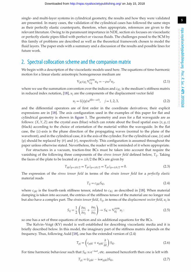
2. Spectral collocation scheme and the companion matrixWe begin with a description of the viscoelastic models used here. The equations of time-harmonicmotion for a linear elastic anisotropic homogeneous medium are

∇jKcKL∇symLq uq = −ρω2uj, (2.1)

where we use the summation convention over the indices and cKL is the medium’s stiffness matrixin reduced index notation, [18], uj are the components of the displacement vector field

uj = Uj(y) ei(kz−ωt), j = 1, 2, 3, (2.2)

and the differential operators are of first order in the coordinate derivatives; their explicitexpressions are in [18]. The axis configuration used in the examples of this paper for flat andcylindrical geometry is shown in figure 1. The geometry and axes for a flat waveguide are asfollows: {X, Y, Z} are the crystal axes (blue) which can rotate about the fixed spatial axes {x, y, z}(black) according to the choice of orientation of the material within the waveguide. In the flatcase, the {z}-axis is the phase direction of the propagating waves (normal to the plane of thewavefront), and in the cylindrical case, it is the axis of the cylinder. For the cylindrical case, {x} and{y} should be replaced by {θ} and {r}, respectively. This configuration is assumed throughout thepaper unless otherwise stated. Nevertheless, the reader will be reminded of it where appropriate.

For structures in a vacuum, traction-free BCs must be taken into account that require thevanishing of the following three components of the stress tensor field defined below, Tij. Takingthe faces of the plate to be located at y = ±h/2 the BCs are given by

Tyy|y=±h/2 = Tyx|y=±h/2 = Tyz|y=±h/2 = 0. (2.3)

The expression of the stress tensor field in terms of the strain tensor field for a perfectly elasticmaterial reads

Tij = cijklSkl, (2.4)

where cijkl is the fourth-rank stiffness tensor, related to cKL as described in [18]. When materialdamping is taken into account, the entries of the stiffness tensor of the material are no longer realbut also have a complex part. The strain tensor field, Sij, in terms of the displacement vector field, uj is

Sij = 12

(∂ui

∂xj+ ∂uj

∂xi

)→ SK = ∇sym

Kj uj : (2.5)

so one has a set of three equations of motion and six additional equations for the BCs.The Kelvin–Voigt (KV) model is well established for describing viscoelastic media and it is

briefly described below. In this model, the imaginary part of the stiffness matrix depends on thefrequency. Thus, following Auld [18], one has the extended version of (2.4)

Tpj =(

cpjkl + κpjkl∂

∂t

)Skl. (2.6)

For time harmonic behaviour such that Skl ∝ e−iωt, etc. assumed henceforth then one is left with

Tpj = (cpjkl − iωκpjkl)Skl, (2.7)



6


...................................................

propagationdirection

hx(r)

x(r)z

y(q)

y(q) z

Figure 1. Geometry and axes for flat plate: {X , Y , Z} are the crystal axes which can rotate about the fixed plate axes {x, y, z}according to the choice of orientation of the material within the plate. In the flat case, the {z}-axis is the phase directionof the propagating waves (normal to the plane of the wavefront), and in the cylindrical case it is the axis of the cylinder.For the cylinder, the figure would represent a longitudinal cross-section in which {x} and {y} should be replaced by {θ} and{r}, respectively. (Online version in colour.)

the viscoelastic stiffness matrix is defined as

cKVpjkl ≡ cpjkl − iωκpjkl. (2.8)

Note that κpjkl has units of sPa, not Pa as cpjkl; to have the same units in both entries and avoidpossible confusion the following tensor is defined:

κpjkl ≡ ηpjkl

ω, (2.9)

where ω is the normalization frequency at which the damping constants of the material weremeasured. This yields the familiar expression for the stiffness matrix with homogeneous units:

cKVpjkl = cpjkl − i

ω

ωηpjkl, (2.10)

where cpjkl and ηpjkl have the same units and the prefactor ω/ω is non-dimensional.The second model considered is the Hysteretic (H) model that is a simplification of

the previous one. In this model, one takes the viscoelastic stiffness matrix to be frequencyindependent:

cHpjkl = cpjkl − iηpjkl. (2.11)

Further discussion of these models is in [13,18,38] and references therein.The SCM scheme for viscoelastic materials is similar to that used for their perfectly elastic

counterparts, see for instance [21,22]. The novelty in the present case, with respect to the studyfor elastic materials presented in [21], is that the SCM will be deployed to search for complexvalues of the wavenumber k rather than real ones as in the perfectly elastic case and this hasconsequences in how the SCM is implemented as described in the next paragraphs. In fact, as hasalready been emphasized, in the perfectly elastic case, the real value of k is fixed and one solvesthe eigenvalue problem for the real values of frequency. This was more convenient in perfectlyelastic cases because the frequency only enters the equations in one term of the PDE so they canbe directly recast into a general eigenvalue problem.

In the case of viscoelastic materials, it is better to fix a real frequency (one-dimensional space)and solve for the complex values of k (two-dimensional space) that satisfy the dispersion equation.The issue now is that k does not enter linearly into the equations of motion. This appears to makeit impossible to recast them into a general eigenvalue problem but an algebraic manipulationknown as the Linear Companion Matrix method allows for this to be rearranged into the moreconvenient form of a general eigenvalue problem. This is achieved at the cost of doubling thedimension of the matrices involved, see Bridges & Morris [44] and references therein for furthermathematical details about this method and their impact on the eigenvalues computation. Morerecently, other authors have successfully used this approach in guided wave problems, see



7


...................................................

Pagneux & Maurel [45] or Postnova [46] for instance. This success has motivated the choice ofthis linearization scheme and as the results have been satisfactory an extension to other schemeshas not been pursued. A brief outline of the manipulations is given in the following paragraph.It must be noted that this manipulation has only been performed in the SCM scheme.

For the viscoelastic case, the equations of motion (2.1) and BCs (2.3) are recast into a generaleigenvalue problem by the standard SCM procedure: we discretize and substitute the derivativesby differentiation matrices (DMs) computed owing to the Matlab suite provided by [47].For a single layer in a vacuum, as we have a bounded interval, the appropriate choice is to useChebyshev DMs, based on a non-uniform Chebyshev grid of N points, these are N × N matrices;the generation of DMs is covered in [42,47]. The mth derivative with respect to y is approximatedby the corresponding mth order Chebyshev N × N DMs:

∂ (m)

∂y(m)�⇒ D(m) := [DMCheb](m)

N×N . (2.12)

The above substitution is made in the equations of motion (2.1), and BCs (2.3), yielding theirmatrix analogue that is succinctly written as

L(k)U = ω2MU (2.13)

and

S(k) :=

⎛⎜⎝TA TB TC

TD TE TF

TG TH TI

⎞⎟⎠⎛⎜⎝U1

U2U3

⎞⎟⎠=

⎛⎜⎝0

00

⎞⎟⎠ , (2.14)

respectively, where U is the vector of vectors: U = [U1, U2, U3]T, these vectors Ui are the componentsof the displacement vector field. The matrix L(k) contains the differential operators of the PDEsand the matrix M is the identity multiplied by −ρ. The BCs in equation (2.3) are taken into accountby appropriately substituting the corresponding rows of (2.13) by those of (2.14) in the followingfashion: the 1, N, (N + 1), 2N, (2N + 1) and 3N rows of the L matrix have been replaced with thoseof the matrix equation S for the BCs of (2.14). Similarly, we replace the same rows of the matrix M

on the right-hand side with rows filled with zeroes. The resultant system has both the governingequation and BCs incorporated in a consistent manner and furthermore has the structure of astandard generalized eigenvalue problem ideally suited for coding. This scheme can be extendedto multi-layer systems but a description of the procedure will not be pursued in this paper becauseit follows exactly the procedure set out in [21] with no need for modifications specific to thedamped cases.

The L(k) matrix contains terms proportional to k0, k1 and k2. Let us rearrange the terms in thematrix equation (2.13) and decompose the L(k) matrix in such a way that the k dependence of thedifferent terms becomes more apparent. One can write(

Q2k2 + Q1k + Q0(ω2))

U = 0. (2.15)

It should be clear now that, once we fix the value of ω, this does not have the structure of ageneral eigenvalue problem in k. To achieve this the following definitions are required. Let U bethe companion displacement vector field:

U ≡ kU. (2.16)

The companion matrices to (2.15) are

M1 ≡(

−Q1 −Q0I Z

)and M2 ≡

(Q2 ZZ I

), (2.17)

where I is the identity matrix and Z is a matrix of zeroes. With the above definitions,equation (2.15) is more conveniently expressed as

M1

(UU

)= k M2

(UU

). (2.18)



8


...................................................

Equation (2.18) is easily solved using an eigensolver routine that yields the complex eigenvaluesk. Regarding the computational resources, we use the routine eig of Matlab (v. R2012b) on an HPdesktop computer. Detailed numerical comparisons and studies of the SCM have been alreadycarried out in [21,22], the reader is referred to these papers for more details on convergenceand accuracy.

To better process the results obtained and retain only the propagating modes which are theobject of study in the present paper, a ratio between the real and imaginary parts of k = α + iβis defined

R ≡ β

α. (2.19)

After the eigenvalues k have been found, R is used to select only those with a low value ofattenuation within the range of wavenumbers under study, these are the propagating modes.Here, the propagation direction of the harmonic perturbation is taken in the positive direction ofthe {z}-axis, the displacement vector field was taken to be proportional to U ∼ eikz in equation (2.2),therefore, β ≥ 0 to ensure the decay of U with distance.

3. The semi-analytical finite-element models for validation of resultsThe SAFE method is popular for studying properties of guided waves along waveguides witharbitrary cross-section, such as railway lines [48], beams [49,50], welded [51] or stiffened plates[52], etc. It uses FEs to represent the cross-section of the waveguide, plus a harmonic descriptionalong the propagation direction, thus limiting the FE model to two dimensions. SAFE analysiscan be deployed using specific programming [38], or advanced use of a flexible commercial codesuch as COMSOL (2014). In this paper, a method described by Predoi et al. [53] is implemented tovalidate results from the SCM method.

The SAFE method assumes that there is no geometric variation of the cross-section along theaxis of the waveguide, so the behaviour in the wave propagation direction can be written inanalytical form. Thus, the displacement vector in the waveguide is written as

uj(x, y, z, t) = Uj(x, y) ei(kz−ωt), (3.1)

in which k is the wavenumber, ω = 2π f is the angular frequency, f is the frequency, t is the timevariable and the subscript j = 1, 2, 3. The function Uj represents the behaviour in the cross-sectionof the waveguide, for which the geometry is irregular, such that it is incorporated in the modelby a two-dimensional FE discretization. For general anisotropic media, the equation of dynamicequilibrium is written in the following form of an eigenvalue problem:

ciqjl∂2Uj

∂xq∂xl+ I(ci3jq + ciqj3)

∂(kUj)

∂xq− kci3j3(kUj) + ρω2δijUj = 0 (3.2)

with summation over the indices j = 1, 2, 3 and q, l = 1, 2. The coefficients cijkl are the stiffnessmoduli and δij is the Kronecker symbol. The equation is reconstructed and solved in the format ofa standard eigenvalue problem in the commercial FE code COMSOL (2014), and the full detailsare provided in [53].

The geometry is meshed by square elements of second order, with side length of 0.05 mm.Periodic BCs [53] were imposed at the lateral boundaries of the domain in the plate models. Thenumber of degree of freedom in our models is less than 11 000, and the typical calculation timefor each SAFE model on a standard PC (Intel Core i7, 8 GB memory) was less than 15 s. Theconvergence has been checked in the models used in our paper, and the results are satisfactory. Infact, this implementation of the SAFE model has already been validated in multi-layer structures[54] as well as solid–fluid structures [55] in which there is a strong impedance contrast. For chosenvalues of angular frequency ω, eigenvalues of complex wavenumber k are found, in which the realpart describes the harmonic wave propagation while its imaginary part presents the attenuation.Each solution at a chosen frequency reveals the wavenumbers of all possible modes at thatfrequency; then the full dispersion curve spectrum is constructed by repeating the eigenvalue



9


...................................................

Kelvin–Voigt orthorhombic 1 mm plateLamb and SH modes

(a) (b)

10 75

50

25

5

00

00

1

SCMSAFE

2 3 4 5 1 2 3 4 5frequency thickness (MHz mm)

phas

e ve

loci

ty (

m m

s–1)

atte

nuat

ion

(Np

m–1

)

frequency thickness (MHz mm)

Kelvin–Voigt orthorhombic 1 mm plateattenuation Lamb and SH modes

Figure 2. Lamb and SH modes phase velocity (a) and attenuation (b) for a 1 mm thick free viscoelastic orthorhombic platewith Kelvin–Voigt-type damping: SCM (circles) versus SAFE (asterisks). Geometry and spatial axes configuration as in figure 1:propagation is along the {Z}-axis, and the {Y}-axis is perpendicular to the plane of the plate. (Online version in colour.)

solutions over the desired range of frequencies. In the following sections, SAFE models will beapplied to both flat and cylindrical structures, and the results are used for validation of thoseobtained by the SCM.

4. Flat geometryIn this section, some illustrative examples in flat geometry are presented. Orthorhombic materialsare treated firstly as a preparatory example because they have already been studied in theliterature (see references). Then, a few novel cases of the most general choice of anisotropicmaterial, triclinic, are presented and the section finishes with a multi-layer example.

Orthorhombic materials are commonly encountered in industry and have already been studiedin two references given in the introduction, namely [32,38]. In the SCM context, a code for anorthorhombic medium can also be used for all those materials whose stiffness matrix has asimilar block structure, such as hexagonal or isotropic; we begin by presenting an example ofa viscoelastic orthorhombic plate in vacuum. The thickness of the plate is 1 mm, the propagationtakes place along the {Z} crystal axis and the {Y} crystal axis is perpendicular to the plane of theplate. More details about the physical properties of this plate are given in the appendix at the end.This example has been done using the Kelvin–Voigt model described in the previous section andthe parameter R = 0.5 for both Lamb and SH modes.

The aforementioned first case is presented in figure 2a,b that show the phase velocity curvesand the attenuation of the Lamb and SH modes, respectively. The comparison between the resultsgiven by the SCM (blue circles) and those given by the corresponding SAFE simulation (redasterisks) is excellent. In figure 3, a detail of figure 2a is shown, and some spurious solutions foundby the SAFE simulation are clearly seen, which are pleasingly not given by the SCM approach.

The next case presented is a 1 mm thick viscoelastic triclinic plate using the Kelvin–Voigtmodel. The propagation takes place along the {Z} crystal axis and the {Y} crystal axis isperpendicular to the plane of the plate. Figure 4a features the dispersion curves and figure 4b,the attenuation for this case. The solution given by the SCM (blue circles) is compared with thatgiven by SAFE (red circles) and the agreement between both solutions is very good. This caseis of particular importance because triclinic materials are the most general type of anisotropicmaterial; with 21 independent constants and only one centre of symmetry which imposes norestriction over the stiffness constants this case poses a great challenge for PWRF routines becauseof its complicated dispersion relation. In [56], the reader can find a brief discussion about these



10


...................................................

phas

e ve

loci

ty (

mm

s–1)

frequency thickness (MHz mm)

6

5

SCMSAFE

4

32 3 4 5

detail of figure 2Lamb and SH modes

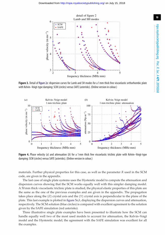
Figure 3. Detail of figure 2a: dispersion curves for Lamb and SH modes for a 1 mm thick free viscoelastic orthorhombic platewith Kelvin–Voigt-type damping: SCM (circles) versus SAFE (asterisks). (Online version in colour.)

Kelvin–Voigt model1 mm triclinic plate

(a) (b)

10SCMSAFE

100

75

50

25

5

1 2 3 4 5 1 2 3 4 5

Kelvin–Voigt model1 mm triclinic plate: attenuation

phas

e ve

loci

ty (

m m

s–1)

atte

nuat

ion

(Np

m–1

)

frequency thickness (MHz mm) frequency thickness (MHz mm)0

00

0

Figure 4. Phase velocity (a) and attenuation (b) for a 1 mm thick free viscoelastic triclinic plate with Kelvin–Voigt-typedamping: SCM (circles) versus SAFE (asterisks). (Online version in colour.)

materials. Further physical properties for this case, as well as the parameter R used in the SCMcode, are given in the appendix.

The last case of single plate systems uses the Hysteretic model to compute the attenuation anddispersion curves showing that the SCM works equally well with this simpler damping model.A 50 mm thick viscoelastic triclinic plate is studied, the physical elastic properties of this plate arethe same as the one of the previous examples and are given in the appendix. The propagationtakes place along the {Z} crystal axis and the {Y} crystal axis is perpendicular to the plane of theplate. This last example is plotted in figure 5a,b, displaying the dispersion curves and attenuation,respectively. The SCM solution (blue circles) is compared with excellent agreement to the solutiongiven by the SAFE simulation (red asterisks).

Three illustrative single plate examples have been presented to illustrate how the SCM canhandle equally well two of the most used models to account for attenuation, the Kelvin–Voigtmodel and the Hysteretic model; the agreement with the SAFE simulation was excellent for allthe examples.



11


...................................................

hysteretic model50 mm triclinic plate

(a) (b)

10 1.0

0.8

0.6

0.4

0.2

9SCMSAFE

87654321

1 2 3 4 5 1 2 3 4 5

phas

e ve

loci

ty (

mm

s–1)

atte

nuat

ion

(Np

m–1

)

hysteretic model50 mm triclinic plate: attenuation

frequency thickness (MHz mm) frequency thickness (MHz mm)0

00

0

Figure 5. Phase velocity (a) and attenuation (b) for a 50-mm thick free viscoelastic triclinic platewith hysteretic-type damping:SCM (blue circles) versus SAFE (red asterisks). Geometry and spatial axes configuration as in figure 1: propagation is along the{Z}-axis, and the {Y}-axis is perpendicular to the plane of the plate.

hysteretic modelmulti-layer plate system

(a) (b)

5

4

SCMSAFE

3

2

1

00

00

5

4

3

2

1

1 2 3 4 5 1 2 3 4 5

phas

e ve

loci

ty (

m m

s–1)

atte

nuat

ion

(Np

m–1

)

hysteretic modelmulti-layer plate system: attenuation

frequency thickness (MHz mm) frequency thickness (MHz mm)

Figure 6. Phase velocity (a) and attenuation (b) for a three-layered system with hysteretic-type damping: viscoelastic 8 mmthick triclinic layer (top), viscoelastic 5 mm thick orthorhombic layer (middle) and elastic 3 mm thick triclinic layer (bottom).Note that the total thickness has been used for the x-axis in the figure. The solutions are plotted as follows: SCM (circles) versusSAFE (asterisks). (Online version in colour.)

This section is closed with a multi-layer example shown in figure 6a,b. The system is composedof three plates: the top plate is 8 mm thick and it is made of a viscoelastic triclinic material, themiddle plate is 5 mm thick and it is made of a viscoelastic orthorhombic material and the bottomplate is a 3 mm thick perfectly elastic triclinic layer. Note that the total thickness has been used forthe x-axis in both figures. The materials of all three layers are different and the physical parametersof the system are retrieved from the appendix. In all the layers, the propagation takes place alongthe {Z} crystal axis and the {Y} crystal axis is perpendicular to the plane of the plate, crystal andspatial axes are aligned and the Hysteretic model was chosen to account for the damping in thematerials. Figure 6a displays the dispersion curves and figure 6b the attenuation. The solutionsgiven by the SCM (blue circles) are once more validated with those given by the SAFE simulation(red asterisks) showing good agreement.

It should be noted that the first case of the section studying orthorhombic materials involvedpropagation along a principal axis and nothing explicit has been said about propagation at anarbitrary angle with respect to the principal axis which can also be seen as a case of monoclinic



12


...................................................

material with propagation within its plane of symmetry, see for instance [7]. This case as well asthe even more general one of a monoclinic material with propagation direction at an arbitraryangle with respect to the plane of symmetry, which after rotation yields a triclinic stiffnessmatrix, can be solved by employing the codes for triclinic materials which have been studiedand validated here. Therefore, for the sake of brevity, these ‘particular’ cases have not beenstudied explicitly and attention has been given only to the general triclinic case containing themas limiting cases.

5. Cylindrical geometryFor the cylindrical geometry, with guided waves propagating along the {Z} crystal axis, thesolutions are classified according to their circumferential harmonic order: n. In general, the solutionshave the following form:

uj = Uj(r) ei(kz+nθ−ωt); j = r, θ , z. (5.1)

In materials such as isotropic or orthorhombic, the solutions with n = 0 yield two decoupledindependent modes, we refer the reader to [21] for the procedure to find out whether there isdecoupling of modes or not in the different materials. These modes are known in the literatureas Torsional and Longitudinal modes, see [17] or [18] for instance. The former are the cylindricalanalogues of the plate SH modes, the latter are the analogues of the plate Lamb waves. In theliterature (see previous references), the solutions with n = 0 are called Flexural modes. Thedifferent families are labelled by the circumferential harmonic order, n. Note that in materials suchas monoclinic or triclinic the splitting of the n = 0 family into Torsional and Longitudinal modesdoes not take place because of their lower degree of symmetry so we simply call them Flexuralmodes of order n = 0. Unless otherwise stated, in the following examples the propagation is alongthe {Z} crystal axis. The crystal axes are also aligned with those of the cylinder as described in §2and shown in figure 1.

The SCM codes for viscoelastic materials in cylindrical geometries are validated in exactly thesame way as their perfectly elastic analogues: by taking the thin plate limit making the internalradius of the cylinder very large compared with its thickness, and comparing the results withthose of a plate of equal properties. This procedure was explained in detail and illustrated withexamples for all types of cylindrical solutions, including circumferential propagation, in [21]. Forthe cases presented in this paper, the same testing procedure was followed and the reference caseswere those presented in the previous section which comprise all types of anisotropic materials andhave been successfully validated with the SAFE method.

It is also interesting to see the agreement between the results given by the SCM and SAFEwhen the thin plate limit is not taken. In figure 7a,b, a comparison between the results givenby the SCM and SAFE is presented. It is a viscoelastic hexagonal cylinder with inner radiusri = 50 mm, thickness h = 15 mm and axial propagation. The Kelvin–Voigt model has been chosenfor modelling the material damping of this case. The figure only displays a short range offrequencies because the number of modes present for higher frequencies increases enormouslyand this renders the comparison of both solutions unclear. The modes computed by the SCMhave been plotted with squares of different colours according to the family to which they belong:n = 0 in black squares, n = 1 in blue squares, n = 2 in red squares and n = 3 in green squares. Thesolution computed by SAFE is plotted in asterisks with the same colour scheme as above. Notethat the SCM gives the results for each family separately, once we have fixed the value of n thecode computes only the modes belonging to that family.

Because of the central role played by fibre reinforced composites in the industry, this sectionis closed with an example of a hexagonal (transversely isotropic) viscoelastic material, suchas is found in fibre-reinforced composites. An interesting and challenging problem for moreconventional approaches such as PWRF routines, though not for the SCM, is the case of acomposite where the fibres along the {Z}-axis of the crystal were chosen to form an angle of 35◦with the axis of the cylinder, this angle does not correspond to any symmetry of the hexagonal



13


...................................................

viscoelastic Kelvin–Voigt hexagonal cylinder flexural modes:SCM (squares) versus SAFE (circles)

(a) (b)

12 0.03

0.02

0.01

11109876543210

00

00.1 0.2 0.3 0.1 0.2 0.3

frequency thickness (MHz mm) frequency thickness (MHz mm)

phas

e ve

loci

ty (

mm

s–1)

atte

nuat

ion

(Np

m–1

)

viscoelastic Kelvin–Voigt hexagonal cylinder attenuation:SCM (squares) versus SAFE (circles)

Figure 7. Phase velocity of flexural modes (a) and attenuation (b). Comparison between SCM and SAFE for a free Kelvin–Voigt-type viscoelastic hexagonal 15 mmthick cylinder of inner radius 50 mm.SCM:n= 0 (black squares),n= 1 (blue squares),n= 2 (red squares) and n= 3 (green squares). SAFE: asterisks with the same colour scheme as for the SCM. Fibres andpropagation along the {z}-axis of the cylinder.

8

transversely isotropic cylinder, fibre at 35°longitudinal n = 0 modes

transversely isotropic cylinder, fibre at 35°longitudinal n = 0 attenuation

7

6

5

4

3

2

1

00

00

1 3 4 52frequency thickness (MHz mm)

1 3 4 52frequency thickness (MHz mm)

phas

e ve

loci

ty (

m m

s–1)

0.2

0.4

0.6

0.8

1.0

1.2

1.4

1.6

atte

nuat

ion

(Np

m–1

)

(a) (b)

Figure 8. SCM solution for the phase velocity of flexural (n= 0) modes phase velocity (a) and attenuation (b) in hexagonal(transversely isotropic) viscoelastic 7 mm thick cylinder of 20 mm inner radius. Kelvin–Voigt-type material damping and fibresat 35◦ with respect to the propagation direction along the {z}-axis of the cylinder.

system. Thus, the fibres follow a helical path around the axis of the cylinder. The cylinder hasinner radius ri = 20 mm, thickness h = 7 mm and the propagation is along the axis of the cylinder.The dispersion curves and attenuation for the family n = 0 using the SCM are shown in figure 8a,b,respectively. This example was done with the Kelvin–Voigt model for damping and the physicalparameters for this example are given in the appendix at the end.

6. Pipes containing fluidsOwing to the importance of pipes filled with fluids in various sectors of industry, NDE engineersneed to have robust tools to perform studies on them and obtain the necessary information aboutmodes that propagate and of their peculiarities. The examples shown in this section deal withviscous fluids as well as with ideal fluids in viscoelastic or elastic pipes, the different modelssuitable to describe the fluid are also discussed. They are validated by comparison to relevantexamples from the literature and to results obtained by using the PWRF approach. Because of the



14


...................................................

way the implementation of the SCM is done to handle cases with material damping, the pipes canbe chosen to be elastic or viscoelastic; therefore, throughout this section, the reader should bearin mind that whenever we encounter an example of elastic pipe, it is equally possible to study itsviscoelastic counterpart using exactly the same code and vice versa. To better study the effects offluid viscosity and material damping, these two mechanisms are isolated from each other in thestudy cases. The section closes with a more general and illustrative example of an orthorhombicpipe with viscous fluid inside.

Before presenting the results, a brief discussion about the different approaches to fluidviscosity and their effects on the results is given. In the context of guided wave NDE, the mostestablished model for viscous fluids regards them as hypothetical solids. For constructing thishypothetical solid two main alternatives have been proposed. The first alternative consists ofsimply regarding the fluid as a true solid with the appropriate stiffness constants: the real part ofshear elastic modulus μ must be taken to be zero, because in the absence of viscosity one mustrecover the case of ideal fluids that do not support shear waves; also the imaginary part of thelongitudinal elastic modulus λ is set to zero because viscosity is assumed to arise solely fromshear motion. The stiffness matrix entries are exactly the same as those of an isotropic solid. In thesecond alternative, λ and μ are taken as in the previous one, but the contribution of the viscosity(non-zero imaginary part of μ) is split among the stiffness matrix entries differently than usuallydone in solid mechanics. Viscosity also enters in those entries with only longitudinal contribution,this model is often referred to as the Stokes model. A more detailed discussion is in [57] andthe equations for these models can be retrieved in [33]. A final comment about the two modelsdescribed above: as explained in [57] the numerical results given by each of the models will differin general. As there is no solid conceptual reason for choosing a priori one or the other model,which of them is more suitable in a particular case is determined by the results from experimentsor other measurements obtained in similar cases.

The first cases studied in this section are pipes with viscous fluid inside. Without loss ofgenerality, the pipes will be elastic so that the attenuation is solely caused by the viscosity ofthe fluid. The dynamical viscosity η for most fluids of interest ranges from orders of 10−1 (verylow viscosity fluids) to 10+1 (high viscous fluids), and in all cases the coefficients representingthis viscosity are several orders of magnitude smaller than those of the elastic solids. When theproblem, pipe and fluid, is described by displacement fields, spurious modes are present becauseof the numerical ill conditioning caused by the big differences among terms in the equationsproduced in turn by the difference in orders of magnitude of the constants entering the problem.One avoids this by turning to a mixed description of the problem using potentials in the fluidlayer and displacements in the solid layer. This enables a homogenization of the terms in theequations of motion of the fluid without any loss of generality regarding the solid layer: recallthat a potential description of anisotropic solids is not possible so the displacement descriptionis necessary lest generality is lost. A similar issue was also found in elastic pipes with idealfluids, see [21].

As the potential description can also be used for isotropic solid materials, the first examplecomputes the longitudinal modes of a hypothetical viscoelastic brass solid rod of radiusri = 23 mm coated with a layer of elastic steel of thickness h = 5 mm; the hysteretic model hasbeen chosen to account for material damping within the solid rod and the propagation takesplace along the axis of the pipe. This case serves as a testbed for the SCM code that is validatedby comparison with results given by the PWRF approach. This case is chosen for its numericalsimplicity, as all the elastic constants involved are of similar orders of magnitude and it is notquite as challenging as that of viscous fluids.

The dispersion curves and the attenuation of the modes is shown in figure 9a,b, respectively.The results given by the SCM are shown in red circles and the solution given by the PWRFapproach is shown in black solid lines. The agreement between both approaches is excellent.

The next two examples show the agreement of the results given by the SCM code just validatedwhen used for modelling viscous fluids with those given in [58]. In the following two cases, theStokes model is assumed throughout to model the viscous fluid. The first example in figure 10



15


...................................................

phas

e ve

loci

ty (

m m

s–1)

(a) (b)

0

0.5

1.5

1.0

0.05 0.10

brass lossy rod coated with steel: dispersion curvesSCM (diamonds) versus PWRF (solid lines)

brass lossy rod coated with steel: attenuationSCM (diamonds) versus PWRF (solid lines)

015frequency (MHz)

0.250.20 0.05 0.10 015frequency (MHz)

0.250.20

2

00

0

4

6

8

10

atte

nuat

ion

(Np

m–1

)

Figure 9. Phase velocity (a) and attenuation (b) of longitudinal modes of a viscoelastic brass rod (ri = 23 mm) coated with anelastic 5 mm thick layer of steel: SCM (circles) versus PWRF (solid lines). (Online version in colour.)

0.8

0.9

1.0

1.1

1.2

0.35 0.40 0.45 0.50frequency (MHz)

steel pipe filled with glycerol with the SCMattenuation

0.55 0.60

h = 1.1 Pa sh = 0.94 Pa sh = 0.8 Pa s

0.65 0.70

atte

nuat

ion

(Np

m–1

)

Figure 10. Attenuation of longitudinal modes in a 0.5 mm thick elastic steel pipe with 4.5 mm inner radius for three differentvalues of the viscosity of glycerol filling the pipe. For the SCM solution: η = 0.8 Pa s (black squares), η = 0.94 Pa s (reddiamonds) and η = 1.1 Pa s (blue circles). In the background, fig. 11 of [58] is displayed. The predictions given by DISPERSEare given in solid lines and the black solid squares are the results from the experiment carried out and described in the paper.

shows a more detailed comparison of the attenuation curves of longitudinal modes propagatingalong the axis of the pipe obtained with the SCM solution to the PWRF solution given in fig. 11of [58]. The pipe is made of steel with inner radius ri = 4.5 mm and thickness h = 0.5 mm. Thefluid is glycerol, the solutions given by the SCM for the viscosities η = 0.8 Pas, η = 0.94 Pas andη = 1.1 Pas are shown in black hollow squares, red diamonds and blue circles, respectively. Thecorresponding PWRF solutions in solid black lines are indicated by the arrows in the backgroundfigure taken from the reference [58], the black solid squares are the experimental results obtainedin the experiment described therein. The SCM solution shows excellent agreement not only withthe PWRF solution but also with the experimental data shown in solid black squares.

The second example in figure 11 computed by the SCM displays the attenuation curve forone longitudinal mode propagating along the axis of a steel pipe with the same properties asbefore filled with a Cannon VP8400 fluid of viscosity η = 18.8 Pa s. The solid black squares in thebackground corresponding to fig. 14 of [58] display experimental results and the solid black line(lying between the two dashed lines) corresponds to the solution for the same value of viscosity



16


...................................................

steel pipe filled with Cannon VP8400 with the SCMattenuation

atte

nuat

ion

(Np

m–1

)

frequency (MHz)

10

9

8

7

6

5

4

3

20.45 0.50 0.55 0.60 0.65 0.70 0.75

h = 18.8 Pas

Figure 11. Attenuation of a longitudinal mode in a 0.5 mm thick elastic steel pipe with 4.5 mm inner radius filled with a fluid:Cannon VP8400. For the SCM solution: η = 18.8 Pa s (circles). In the background, fig. 14 of [58] is displayed. The predictionsgiven by DISPERSE are given in solid lines (between the dashed lines) for the same viscosity value ofη = 18.8 Pa s. The dashedlines correspond to close but different values of viscosity, see [58] for more details. The black solid squares are the results fromthe experiment carried out and described in the paper. (Online version in colour.)

η = 18.8 Pa s obtained with DISPERSE. The dashed lines correspond to close but different valuesof viscosity, more details of this figure are in the original reference [58]. Once again, the solutiongiven by the SCM shows excellent agreement with both experiment and PWRF prediction.

The above examples were also run using the true solid model described at the beginning, forbrevity not shown here. As a consequence of the different splitting of the viscosity among theentries of the stiffness matrix, it was seen that the peaks appearing in the attenuation curves werelower than those yielded by the Stokes model. In the regions of the spectrum where experimentalresults were available, the solution given by the true solid model agrees very well with them,though it was not as good a match as with the Stokes model.

All the cases studied in this section involved a perfectly elastic pipe with either a viscoelasticsolid or a viscous fluid filling the inside. Figure 12a,b show, respectively, the dispersion curves andattenuation of longitudinal modes propagating along the axis of a viscoelastic steel pipe of innerradius ri = 30 mm and thickness h = 8 mm filled with water (modelled as an ideal fluid withoutviscosity). The solution given by the SCM is given in red circles and that computed by the PWRFmethod in solid black lines. Both solutions show very good agreement and can be comparedwith the perfectly elastic analogue in [21], thus showing that low material damping has littleeffect on the dispersion curves. The hysteretic model is used in this case and the values of theviscoelastic constants of the pipe are in the appendix. Note that the solution given by the PWRFis not complete, some of the curves had to be traced manually and even after some work it wasvery difficult to find the incomplete intervals. This highlights one of the advantages of the SCM,namely completeness of solutions, over conventional PWRF routines.

This section concludes with a brief comment on the ill-conditioning of the SCM whenstudying problems involving fluids of very low viscosity. It has been found in the courseof this investigation that for viscosity values of the order of ∼0.1 Pa s or less, some piecesof the dispersion curves and the corresponding mode shapes obtained in the region close tozero frequency are not as smooth as one normally observes in more simple problems. Thisphenomenon has been observed in a variety of different combination of materials and geometricparameters which suggests it is an inherent feature of the SCM when used to model fluids whichlie at the frontier between ideal and viscous fluids. However, a useful trend has been observed:



17


...................................................

0.05

0.10

0.15

0.20

0.25

0.30

0.35

0.40

0.45

0.50

0 0.05 0.150.10frequency (MHz)

lossy steel pipe filled with water: dispersion curvesSCM (diamonds) versus PWRF (solid lines)

lossy steel pipe filled with water: attenuationSCM (diamonds) versus PWRF (solid lines)

0 0.05 0.150.10frequency (MHz)

1

2

3

4

5

6

7

8

9

10ph

ase

velo

city

(m

ms–1

)

atte

nuat

ion

(Np

m–1

)

(a) (b)

Figure 12. Phase velocity (a) and attenuation (b) of longitudinal modes of an 8 mm thick viscoelastic steel pipe (ri = 30 mm)filledwithwater (ideal fluid): SCM (circles) versus PWRF (solid lines). Hystereticmodel formaterial damping. Propagation alongthe {z}-axis of the pipe. (Online version in colour.)

the higher the viscosity is, the closer one can go towards zero frequency keeping smooth profilesin dispersion curves and mode shapes.

7. Discussion and conclusionIn this paper, an extension of the SCM to guided wave problems in viscoelastic media with thepossibility of containing viscous fluids has been presented. Cases in flat, as well as in cylindrical,geometry have been studied and validated with numerous examples from the literature, solutionsobtained with the conventional PWRF approach and when this approach was not possible, inthe case of triclinic media for instance, a SAFE simulation was used to confirm the results. Asthe wavenumber k entered the equations nonlinearly the Linear Companion Matrix Method wasintroduced to rearrange the problem into a generalized eigenvalue problem.

The SCM shows excellent performance solving guided wave problems in viscoelastic mediaand some of its advantages with respect to the SAFE method or PWRF routines have becomeapparent in the course of the paper and are summarized below. Even though the aforementionedLinear Companion Matrix Method is required to recast the problem into the desired form, the SCMremains conceptually simpler than the SAFE method and the amount of previous knowledgerequired for its implementation is significantly less. As the examples and comments in the §§3and 4 have highlighted, the SAFE simulation used here is known to give solutions which donot correspond to plate modes and need to be carefully filtered, mostly by manual intervention.It must be emphasized that other SAFE schemes, using one-dimensional grids for instance [39],can be used for these type of problems in which no non-plate modes in the final results have beenreported so far. This phenomenon has not been observed to occur with the SCM even thoughsome very simple post processing is useful to retain the desired propagating mode solutions. Thishas been done by introducing at the end of §2 the ratio R between the real and imaginary parts ofthe wavenumber. For the cases studied here, the implementation of the method and processingof physical results of the SCM has been found to be invariably easier and more straightforwardthan that with SAFE.

When complex roots must be found the SCM is easier to code than the conventional PWRFroutines because it transforms the set of partial differential equations for the acoustic waves intoa purely algebraic problem, see [21,22] for more details on this important point. In addition, theSCM is generally faster than the PWRF method as it does not require any intervention on thepart of the practitioner who sometimes has to manually complete or find solutions when using



18


...................................................

the PWRF approach. This is because the SCM does not miss any eigenvalues and therefore onecan be certain that the solution is complete and no modes have been missed. Mode missing isa recurrent problem encountered in PWRF routines specially when solving complicated casesinvolving complex roots or anisotropic materials. Finally, the SCM is capable of solving casesthat are not currently solved by PWRF routines such as propagation in anisotropic media in anarbitrary direction as was pointed out at the end of §4 or as the last case in §4 shows.

In conclusion, the SCM presents itself as a powerful and robust complement to the alreadyestablished SAFE and PWRF approaches. The SCM scheme, and the study of guided waves inviscoelastic generally anisotropic media, as presented in this paper is expected to be of interestin very different branches of physics dealing with guided wave phenomena and engineeringapplications working with composite materials and guided waves. Finally, as mentioned in theintroduction, the implementation of the SCM described in this paper can also be used to calculatethe non-propagating solutions, without any further development of the computational method.For brevity, such examples have not been included here.

Data accessibility. The datasets supporting this article have been uploaded as part of the electronic supplementarymaterial. And can also be found in the appendix to be published at the end of the paper.Authors’ contributions. F.H.Q. carried out the simulations and coding of the Spectral Collocation Method (SCM)as well as drafting the paper. Z.F. designed and carried out the SAFE model and simulations with which theSCM was validated and wrote the section of the SAFE method. M.J.S.L. and R.V.C. supervised the project aswell as helped drafting the manuscript and revising.Competing interests. We have no competing interests.Funding. F.H.Q. is supported by a PhD studentship from the NDT group at Imperial College London. Z.F.is an Assistant Professor at Nanyang Technological University (Singapore) and is supported by his owninstitution. Both M.J.S.L. and R.V.C. are Professors at Imperial College London (UK) and are supported bytheir institution.

Appendix A. Numerical dataThe physical and geometrical information used for the figures presented in the main text are givenhere. The number of grid points N varies from one example to another, but it is always at leastdouble the number of modes plotted in the figure. On a practical level N is chosen to achievethe shortest computation time, that is, if one is interested in the first 10 modes, running a codewith N = 100 is unnecessary; a value of N between 25 and 30 has consistently been shown to besufficient.

The parameters for the plate of figure 2a,b are as follows (with the usual axes orientation shownin figure 1):

ρ = 1500 kg m−3; h = 1 mm, (A 1)

h stands for the thickness of the plate. The elastic stiffness matrix is given in GPa

c =

⎛⎜⎜⎜⎜⎜⎜⎜⎝

132 6.9 5.912.3 5.5

12.13.32

6.216.15

⎞⎟⎟⎟⎟⎟⎟⎟⎠

. (A 2)

The viscosity matrix in GPa is

η =

⎛⎜⎜⎜⎜⎜⎜⎜⎝

0.4 0.001 0.0160.037 0.021

0.0430.009

0.0150.02

⎞⎟⎟⎟⎟⎟⎟⎟⎠

. (A 3)



19


...................................................

The parameters for the plate of figure 4a,b are as follows (with the usual axes orientation shownin figure 1):

ρ = 1500 kg m−3; h = 1 mm; f = 2 MHz, (A 4)

h stands for the thickness of the plate and f is the normalization frequency in equation (2.10).The elastic stiffness matrix is given in GPa

c =

⎛⎜⎜⎜⎜⎜⎜⎜⎝

74.29 28.94 5.86 0.20 −0.11 37.1925.69 5.65 0.0928 −0.0801 17.52

12.11 0.0133 −0.0086 0.224.18 1.31 0.0949

5.35 −0.070528.29

⎞⎟⎟⎟⎟⎟⎟⎟⎠

. (A 5)

The viscosity matrix in MPa is

η =

⎛⎜⎜⎜⎜⎜⎜⎜⎝

218 76.5 16.4 −3.60 0.688 11671.1 19.2 −0.771 2.15 50

42.2 −0.9644 0.627 −3.0711.1 2.89 −1.15

13.6 1.4893.5

⎞⎟⎟⎟⎟⎟⎟⎟⎠

. (A 6)

The parameters for the plate of figure 5a,b are the same as above, equations (A 4)–(A 6) exceptfor the thickness which now is h = 50 mm.

The multi-layer system of figure 6a,b is composed of three layers. The top layer has a thicknessof h = 8 mm and the rest of the properties are given in (A 4)–(A 6). The middle layer has a thicknessof h = 5 mm and the other properties are given in (A 1)–(A 3). The bottom layer parameters are asfollows:

ρ = 8938.4 kg m−3; h = 3 mm, (A 7)

h stands for the thickness of the plate. The elastic stiffness matrix is given in GPa

c =

⎛⎜⎜⎜⎜⎜⎜⎜⎝

2.0787 1.0906 0.9341 0.16574 −0.1615 −0.231881.677 1.3624 −0.24719 0.1128 0.086831

1.8591 0.081453 0.082076 0.145051.0023 0.14505 0.058388

0.35110 0.165740.59472

⎞⎟⎟⎟⎟⎟⎟⎟⎠

. (A 8)

The parameters for the cylinder of figure 7a,b are as follows (with the usual axes orientationshown in 1):

ρ = 1605 kg m−3; h = 15 mm; ri = 50 mm; f = 2.242 MHz, (A 9)

h stands for the thickness of the plate and f is the normalization frequency in equation (2.10). Theelastic stiffness matrix is given in GPa

c =

⎛⎜⎜⎜⎜⎜⎜⎜⎜⎝

11.6911464939 5.85222031944 5.6162971550111.6911464939 5.61629715501

130.1959795033.7

3.7c11 − c12

2

⎞⎟⎟⎟⎟⎟⎟⎟⎟⎠

. (A 10)

The viscosity matrix in GPa is given by

ηij = 0.025 cij. (A 11)



20


...................................................

The parameters for the cylinder of figure 8a,b are as follows (with the usual axes orientationshown in 1):

ρ = 2350 kg m−3; h = 7 mm; ri = 20 mm; f = 2.242 MHz, (A 12)

h stands for the thickness of the plate and f is the normalization frequency in equation (2.10).The elastic stiffness matrix is given in GPa

c =

⎛⎜⎜⎜⎜⎜⎜⎜⎜⎝

132 6.9 5.9132 5.9

12.13.32

3.32c11 − c12

2

⎞⎟⎟⎟⎟⎟⎟⎟⎟⎠

. (A 13)

The viscosity matrix in GPa is

η =

⎛⎜⎜⎜⎜⎜⎜⎜⎜⎝

0.4 0.001 0.0160.4 0.016

0.0430.009

0.009η11 − η12

2

⎞⎟⎟⎟⎟⎟⎟⎟⎟⎠

. (A 14)

A rotation of 35◦ about the {r}-axis must performed on these matrices so that the fibres follow anhelicoidal path around the cylinder.

The parameters for the cylindrical system of figure 9a,b are as follows. For the outer elasticsteel cylinder

ρ = 7932 kg m−3; h = 5 mm; ri = 23 mm; cL = 5960 m s−1; cS = 3260 m s−1. (A 15)

The viscoelastic isotropic material in the inner core filling the outer layer of the cylinder has thefollowing physical properties similar to those of brass:

ρ = 4000 kg m−3. (A 16)

The elastic stiffness matrix is given in GPa

c =

⎛⎜⎜⎜⎜⎜⎜⎜⎝

100 50 50100 50

10025

2525

⎞⎟⎟⎟⎟⎟⎟⎟⎠

. (A 17)

The viscosity matrix in GPa is given by

ηij = 0.0025 cij. (A 18)

For the system in figure 10, the parameters for the steel pipe are

ρ = 7932 kg m−3; h = 0.5 mm; ri = 4.5 mm; cL = 5959 m s−1; cS = 3260 m s−1. (A 19)

The fluid inside is glycerol and has the following properties:

ρ = 1258 kg m−3; cL = 1918 m s−1; cS = 0 m s−1. (A 20)

The values for the dynamic viscosity of glycerol for the different curves (see figure 10) are

η1 = 0.8 Pa s; η2 = 0.94 Pa s; η3 = 1.1 Pa s. (A 21)



21


...................................................

For the system in figure 11, the parameters for the steel pipe are the same as for figure 10.The fluid inside is Cannon VP8400 and has the following properties

ρ = 885 kg m−3; cL = 1525 m s−1; cS = 0 m s−1; η = 18.8 Pa s. (A 22)

For the system in figure 12a,b the parameters for the steel pipe are

ρ = 7932 kg m−3; h = 8 mm; ri = 30 mm; cL = 5960 m s−1; cS = 3260 m s−1 (A 23)

and the viscosity matrix is obtained from the stiffness matrix

ηij = 0.0025 cij. (A 24)

The fluid inside is water (treated as an ideal fluid) and has the following properties:

ρ = 1500 kg m−3; cL = 1000 m s−1; cS = 0 m s−1. (A 25)

References1. Mindlin RD. 1960 Waves and vibrations in isotropic, elastic plates. In Structural mechanics (eds

JN Goodier, N Hoff), pp. 199–323. Oxford, UK: Pergamon Press.2. Mindlin RD, Pao YH. 1960 Dispersion of flexural waves in elastic circular cylinder. J. Appl.

Mech. 27, 513–520. (doi:10.1115/1.3644033)3. Pao YH. 1962 The dispersion of flexural waves in an elastic circular cylinder, Part II. J. Appl.

Mech. 29, 61–64. (doi:10.1115/1.3636498)4. Gazis DC. 1958 Exact analysis of the plane-strain vibrations of thick walled hollow cylinders.

J. Acoust. Soc. Am. 30, 786–794. (doi:10.1121/1.1909761)5. Zemanek J. 1972 An experimental and theoretical investigation of elastic wave propagation in

a cylinder. J. Acoust. Soc. Am. 51, 265–283. (doi:10.1121/1.1912838)6. Solie LP, Auld BA. 1973 Elastic waves in free anisotropic plates. J. Acoust. Soc. Am. 54, 50–65.

(doi:10.1121/1.1913575)7. Nayfeh AH, Chimenti DE. 1989 Free wave propagation in plates of general anisotropic

media. In Review of progress in quantitative non-destructive evaluation (eds DO Thompson, DEChimenti), p. 181. New York, NY: Plenum Press.

8. Li Y, Thompson RB. 1990 Influence of anisotropy on the dispersion characteristics of guidedultrasonic plate modes. J. Acoust. Soc. Am. 87, 1911–1931. (doi:10.1121/1.399318)

9. Towfighi S, Kundu T, Ehsani M. 2002 Elastic wave propagation in circumferential direction inanisotropic cylindrical curved plates. J. Appl. Mech. 69, 283–291. (doi:10.1115/1.1464872)

10. Lowe MJS. 1995 Matrix Techniques for modeling ultrasonic waves in multilayered media.IEEE Trans. Ultrason. Ferroelectr. Freq. Control 42, 525–542. (doi:10.1109/58.393096)

11. Nayfeh AH. 1989 The propagation of horizontally polarized shear waves in multilayeredanisotropic media. J. Acoust. Soc. Am. 86, 2007–2012. (doi:10.1121/1.398580)

12. Nayfeh AH. 1991 The general problem of elastic wave propagation in multilayeredanisotropic media. J. Acoust. Soc. Am. 89, 1521–1531. (doi:10.1121/1.400988)

13. Rose JL. 1999 Ultrasonic waves in solid media, pp. 1–476. Cambridge, UK: Cambridge UniversityPress.

14. Kaplunov JD, Kossovich LY, Lee KH. 2000 Dynamics of thin walled elastic bodies, pp. 1–240.New York, NY: Elsevier.

15. Wang CM, Reddy JN, Lee KH. 2000 Shear deformable beams and plates. Relationships with classicalsolutions, pp. 1–312. New York, NY: Elsevier.

16. Rokhlin SI, Chimenti DE, Nagy PB. 2011 Physical ultrasonics of compoistes, pp. 1–378. Oxford,UK: Oxford University Press.

17. Graff KF. 1991 Rayleigh and lamb waves, pp. 1–649. New York, NY: Dover.18. Auld BA. 1990 Acoustic fields and waves in solids, 2nd edn., pp. 1–878. Malabar, FL: Krieger

Publishing Company.19. Achenbach JD. 1973 Wave propagation in elastic solids, pp. 1–440. Amsterdam, The Netherlands:

North-Holland.20. Viktorov IA. 1967 Rayleigh and lamb waves, pp. 1–168. New York, NY: Plenum Press.21. Hernando Quintanilla F, Lowe MJS, Craster RV. 2015 Modelling guided elastic waves in

generally anisotropic media using a spectral collocation method. J. Acoust. Soc. Am. 137,1180–1194. (doi:10.1121/1.4913777)


http://dx.doi.org/doi:10.1115/1.3644033












22


...................................................

22. Adamou ATI, Craster RV. 2004 Spectral methods for modelling guided waves in elastic media.J. Acoust. Soc. Am. 116, 1524–1535. (doi:10.1121/1.1777871)

23. Kreiss HO, Oliger J. 1972 Comparison of accurate methods for the integration of hyperbolicequations. Tellus 24, 199–215. (doi:10.1111/j.2153-3490.1972.tb01547.x)

24. Orszag SA. 1972 Comparison of pseudospectral and spectral approximation. Stud. Appl. Math.51, 253–259. (doi:10.1002/sapm1972513253)

25. Fornberg B. 1975 On a Fourier method for the integration of hyperbolic equations. SIAM J.Numer. Anal. 12, 509. (doi:10.1137/0712040)

26. Karpfinger F, Gurevich B, Bakulin A. 2008 Modeling of wave dispersion along cylindricalstructures using the spectral method. J. Acoust. Soc. Am. 124, 859–865. (doi:10.1121/1.2940577)

27. Karpfinger F, Gurevich B, Bakulin A. 2008 Modeling of axisymmetric wave modes ina poroelastic cylinder using the spectral method. J. Acoust. Soc. Am. 124, EL230–EL235.(doi:10.1121/1.2968303)

28. Karpfinger F, Valero HP, Gurevich B, Bakulin A, Sinha B. 2010 Spectral-method algorithmfor modeling dispersion of acoustic modes in elastic cylindrical structures. Geophysics 75,H19–H27. (doi:10.1190/1.3380590)

29. Kocabas SE, Veronis G, Miller DAB, Fan S. 2009 Modal analysis and coupling in metal-insulator-metal waveguides. Phys. Rev. B 79, 035120. (doi:10.1103/PhysRevB.79.035120)

30. Gridin D, Adamou ATI, Craster RV. 2004 Electronic eigenstates in quantum rings: asymptoticsand numerics. Phys. Rev. B 69, 155317. (doi:10.1103/PhysRevB.69.155317)

31. Nagy PB, Nayfeh AH. 1996 Viscosity Induced attenuation of longitudinal guided waves influid-loaded rods. J. Acoust. Soc. Am. 100, 1501–1508. (doi:10.1121/1.415996)

32. Cawley P, Lowe MJS, Neau G. 2001 Understanding attenuative lamb wave propagation incomposites. London, UK: DERA.

33. Pavlakovic B, Lowe M. 2013 DISPERSE user’s manual, version 2.0.20B, pp. 1–209. London, UK:Imperial College.

34. Pavlakovic B, Lowe M, Alleyne D, Cawley P. 1987 DISPERSE: a general purpose program forcreating dispersion curves. Rev. Progr. Quant. Non-destructive Eval. 16, 185.

35. Simonetti F, Cawley P. 2004 On the nature of shear horizontal wave propagation in elasticplates coated with viscoelastic media. Proc. R. Soc. Lond. A 460, 2197–2221. (doi:10.1098/rspa.2004.1284)

36. Simonetti F. 2004 Lamb wave propagation in elastic plates coated with viscoelestic materials.J. Acoust. Soc. Am. 115, 2041–2053. (doi:10.1121/1.1695011)

37. Bernard A, Lowe MJS, Deschamps M. 2001 Guided waves energy velocity in absorbing andnon-absorbing plates. J. Acoust. Soc. Am. 110, 186–196. (doi:10.1121/1.1375845)

38. Bartoli I, Marzani A, Lanza di Scalea F, Viola E. 2006 Modeling wave propagation indamped waveguides of arbitrary cross-section. J. Sound Vib. 295, 685–707. (doi:10.1016/j.jsv.2006.01.021)

39. Marzani A, Viola E, Bartoli I, Lanza di Scalea F, Rizzo P. 2008 A semi-analytical finite elementformulation for modeling stress wave propagation in axisymmetric damped waveguides.J. Sound Vib. 318, 488–505. (doi:10.1016/j.jsv.2008.04.028)

40. Gottlieb D, Orszag SA. 1977 Numerical analysis of spectral methods: theory and applications,pp. 1–179. Philadelphia, PA: SIAM.

41. Boyd JP. 2001 Chebyshev and fourier spectral methods, pp. 1–688. New York, NY: Dover.42. Trefethen L. 2000 Spectral methods in MATLAB, pp. 1–181. Philadelphia, PA: SIAM.43. Fornberg B. 1996 A practical guide to pseudoespectral methods, pp. 1–231. Cambridge, UK:

Cambridge University Press.44. Bridges TJ, Morris PJ. 1984 Differential eigenvalue problems in which the parameter appears

nonlinearly. J. Comput. Phys. 55, 437–460. (doi:10.1016/0021-9991(84)90032-9)45. Pagneux V, Maurel A. 2001 Determination of Lamb mode eigenvalues. J. Acoust. Soc. Am. 110,

1307–1314. (doi:10.1121/1.1391248)46. Postvova JA. 2008 Trapped modes in non-uniform elastic waveguides: asymptotic and numerical

methods. London, UK: Imperial College London.47. Weideman JAC, Reddy SC. 2000 A MATLAB differentiation matrix suite. ACM Trans. Math.

Softw. 26, 465–519. (doi:10.1145/365723.365727)48. Gavric L. 1995 Computation of propagative waves in free rail using a finite element technique.

J. Sound Vib. 185, 531–543. (doi:10.1006/jsvi.1995.0398)49. Hayashi T, Song WJ, Rose JL. 2003 Guided wave dispersion curves for a bar with an

arbitrary cross-section, a rod and rail example. Ultrasonics 41, 175–183. (doi:10.1016/S0041-624X(03)00097-0)



http://dx.doi.org/doi:10.1111/j.2153-3490.1972.tb01547.x

http://dx.doi.org/doi:10.1002/sapm1972513253

http://dx.doi.org/doi:10.1137/0712040




http://dx.doi.org/doi:10.1103/PhysRevB.79.035120

http://dx.doi.org/doi:10.1103/PhysRevB.69.155317


http://dx.doi.org/doi:10.1098/rspa.2004.1284




http://dx.doi.org/doi:10.1016/j.jsv.2006.01.021



http://dx.doi.org/doi:10.1016/0021-9991(84)90032-9



http://dx.doi.org/doi:10.1006/jsvi.1995.0398

http://dx.doi.org/doi:10.1016/S0041-624X(03)00097-0

http://dx.doi.org/doi:10.1016/S0041-624X(03)00097-0


23


...................................................

50. Wilcox P, Evans M, Lowe MJS, Cawley P. 2002 Dispersion and excitability of guided acousticwaves in isotropic beams with arbitrary cross-section. In Review of progress in quantitative non-destructive evaluation, vol. 21, pp. 203–210 (eds DO Thompson, DE Chimenti). New York, NY:Plenum Press.

51. Fan Z, Lowe MJS. 2009 Elastic waves guided by a welded joint in a plate. Proc. R. Soc. A 465,2053–2068. (doi:10.1098/rspa.2009.0010)

52. Fan Z, Castaings M, Lowe MJS, Biateau C, Fromme P. 2013 Feature-guided waves formonitoring adhesive shear modulus in bonded stiffeners. NDT & E Int. 54, 96–102.(doi:10.1016/j.ndteint.2012.12.006)

53. Predoi MV, Castaings M, Hosten B, Bacon C. 2007 Wave propagation along transverselyperiodic structures. J. Acoust. Soc. Am. 121, 1935–1944. (doi:10.1121/1.2534256)

54. Castaings M, Lowe MJS. 2008 Finite element model for waves guided along solid systems ofarbitrary section coupled to infinite solid media. J. Acoust. Soc. Am. 123, 696–708. (doi:10.1121/1.2821973)

55. Castaings M, Bacon C, Lowe MJS, Fan Z. 2008 Torsional waves propagation along awaveguide of arbitrary cross section immersed in a perfect fluid. J. Acoust. Soc. Am. 124,2002–2010. (doi:10.1121/1.2968677)

56. Nayfeh AH, Chimenti DE. 1989 free wave propagation in plates of general anisotropic media.J. Appl. Mech. 56, 881–886. (doi:10.1115/1.3176186)

57. Nagy PB, Nayfeh AH. 1997 Excess attenuation of leaky Lamb waves due to viscous fluidloading. J. Acoust. Soc. Am. 101, 2649–2658. (doi:10.1121/1.418506)

58. Ma J, Lowe MJS, Simonetti F. 2007 Measurement of the properties of fluids inside pipesusing guided longitudinal waves. IEEE Trans. Ultrason. Ferroelectr. Freq. Control 54, 647–658.(doi:10.1109/TUFFC.2007.288)



http://dx.doi.org/doi:10.1016/j.ndteint.2012.12.006







http://dx.doi.org/doi:10.1109/TUFFC.2007.288


on June 19, 2018 Guidedwaves’dispersion rspa...

Documents

Transcript of on June 19, 2018 Guidedwaves’dispersion rspa...