Electrosmosis between plane parallel walls...

Electrosmosis between Plane Parallel W alls produced by Pligh-Frequency A lternating Currents

B y L. R o sen h ea d , P h .D., D.Sc. and J . C. P. Mil l e r , M.A., P h .D.

(W it h N ote by J. J . B ik e r m a n )

( Communicated by W . C. M. Lewis, — Received 29 June 1937)

1— I ntro du ctio n

The problem of the motion, under the influence of high-frequency alternating currents, of fluid between plane parallel walls whose distance apart is very small, appears to be of interest in certain branches of Physical Chemistry. The following paper contains a mathematical treatm ent of this type of motion under certain specified conditions. We are greatly indebted to Mr. J . J . Bikerman of the Chemistry Departm ent of the University of Manchester for having brought the problem to our notice, and for having given us a great deal of information concerning the physics of the phenomena involved.

In general, when two different substances, or phases, have a common surface, there is an electrokinetic potential difference between them. This is produced by an electric double layer of ions in contact with the common surface. Consider the boundary between a solid and an electrolyte, and let us assume the solid to take a negative charge, as is almost invariably the case when the electrolyte is water or a very dilute aqueous solution. The negative layer consists, probably, of ions adsorbed rigidly to the surface. Near the surface, in the fluid, there will be a preponderance of positively charged ions held more or less firmly in position by electrostatic forces. Very close to the “ rigid” layer of negative ions the electrostatic forces will be sufficiently great to keep the positive ions rigidly in place. As we leave the solid surface the forces diminish and ultimately a position is reached where diffusion and thermal forces overcome the electrostatic forces. Beyond this surface in the fluid there will still be a preponderance of positive ions, since the electrostatic forces will still be operative, but these ions will be mobile. At points remote from the solid surface there are approximately equal concentrations of positive and negative ions, and the liquid as a whole is electrically neutral. The equilibrium attained when electrostatic and diffusion forces are operating was first calculated by Gouy; the expression given by Gouy for the charge density is used in this paper. On applying

• [ 298 ]

on May 28, 2018http://rspa.royalsocietypublishing.org/Downloaded from

http://rspa.royalsocietypublishing.org/

Electrosmosis between Plane Parallel Walls 299

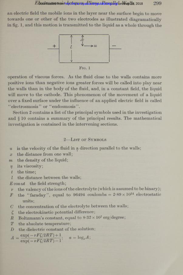
an electric field the mobile ions in the layer near the surface begin to move towards one or other of the two electrodes as illustrated diagramatically in fig. 1, and this m otion is transm itted to the liquid as a whole through the

F ig . 1

operation of viscous forces. As the fluid close to the walls contains more positive ions than negative ions greater forces will be called into play near the walls th an in the body of the fluid, and, in a constant field, the liquid will move to the cathode. This phenomenon of the movement of a liquid over a fixed surface under the influence of an applied electric field is called “ electrosmosis” or “ endosmosis” .

Section 2 contains a list of the principal symbols used in the investigation and § 10 contains a sum m ary of the principal results. The m athem atical investigation is contained in the intervening sections.

2— L ist o f Sym bols

u is the velocity of the fluid in a direction parallel to the walls; x the distance from one wall; m the density of the liquid;7] its viscosity; t the tim e;l the distance between the walls;

E coso)t the field strength;v the valency of the ions of the electrolyte (which is assumed to be b inary);

F the “ fa raday” , equal to 96494 coulombs = 2-89 x 1014 electrostatic u n its ;

C the concentration of the electrolyte between the walls;£ the electrokinetic potential difference;

R Boltzm ann’s constant, equal to 8*32 x 10' erg/degree;T the absolute tem perature;D the dielectric constant of the solution;

exp( — vI^ I2 R T) + 1exp( — vF£/2RT) — 1 ’

logeA;



300 L. Rosenhead and J. C. P. Miller

c x = 2vF(2nC/DRT)i ; n 2 = mco/oc2!};

8vFC g 2gx— — ~is, according to Gouy (1910) and Bikerman (1933),

the volume density of the electric charge in the liquid a t a distance x from a plane wall;

G = EAvFG; H = G/oc2y = EAvFC/oc2y;£ = a(x — P); A = a + \od;

y, P and Q are functions, the last two real functions, of £ (or of x), which are defined in such a way th a t u is the real part of

Heio)ty{E, ) a n d

so th a t u = H(Pcos cot—Q sin ;

yr and f rare functions connected with the expansion of as a series in powers of n2, they are defined in § 5 for r = 0, 1, 2 , . . etc., and their expansions are given in equations (6*2), (6-3), (6-5). They are connected by the relation

Vr — fr(^ + £) + / r(A — £);

Yr is the value of yr when £ = ± \cd ;F(x) and e are defined by means of the relation

u = HF(x) cos

F(x) = (P2 + Q2) is the greatest value of ujH attained at a given value of x\ e = tan_1( — Q/P) is the phase-lag.

The orders of magnitude of some of the above constants, in the range of experiments considered, are given by the following set of approximate values:

rj — 10-2 g./cm.sec.; m = 1 g./cm.3; E = 10~2 gd/cmdsec.; A = T01 to 2 (dimensionless); 8 vFCabout 109gA/cm.fsec.; a — 106 cm.-1; I = 10-4 cm.; co lies between 102 and 105 sec.-1; ccl is greater than 20; lies between 10-5 and 10-8; nod is less than 1 (the last three quantities are dimensionless).

In an electric field of constant strength the highest velocity ( usually observed is less than 5 x 10-3 cm./sec. When l = 10-4, electrical measurements of “ surface conductivity” can be made with an error of ± 3 %, but when l = 10-3 the error is roughly + 20 %.

3— T he E quation and th e Com plem entary Solution

We consider the motion of fluid, between two plane parallel walls whose distance apart is l, under the influence of an applied electric field whose




strength is Ecosa>t. Accepting the formula suggested by Gouy (1910) for the volume density of the electric charge in liquid a t a distance from a plane wall, the equation to be satisfied by u, the velocity of the fluid in a direction perpendicular to x, is

du d2u _ . r 2 A e ax{A2e2ccx+ l} 2Aea(l-^ {A 2e2cc( x> + 1}"] m m ~ Vdx2 ~ {A2e2a* —1 }2 + {A%2a(/-x)_ip _]>

where G = E A v F C . (3-2)

The equation (3*1) is derived from the ordinary equations of motion of a viscous fluid on the assumption (i) th a t the velocities are so small th a t squares and higher powers can be neglected, and (ii) th a t the direction of the motion is parallel to the direction of the applied electric force. (In the experiments under investigation u is never greater than 5 x 10-3 cm./sec.) In the equation the electric force has been w ritten as Eei(ot, and this must be in terpreted as meaning th a t the velocity u is the real part of the solution obtained from (3-1). Further, the boundary conditions to be satisfied by u are

u — 0 a t x = 0 and x — l. (3*3)

Since the equation is linear in u, the solution may be split up into (i) a complem entary solution and (ii) a particular integral. The complementary solution satisfies the equation

mdu d2u d t ~ V dx2 = 0, (3-4)

and it can be shown very easily th a t the only solution of (3-4) which satisfies (3-3) is

u = ZK rex])( — 7jr27T2t/l2m) sm.(rn(3-5)

where the summation is over all integral values of r from 1 to 00, and where each Kr is a constant.

The solution (3*5) represents the free oscillations. I f we substitute 7j = 10-2, l = 10~4, m = 1 c.g.s. units as typical values of the constants, we see th a t these oscillations die away very rapidly. The coefficients of t in the exponentials are always negative, and th a t coefficient which corresponds to r = 1 is the one th a t is numerically least. The coefficient in this case is approximately ( — 107), so th a t the first term in (3-5) diminishes in the ratio 1/e in 10~7 sec.; other terms diminish even more rapidly. We shall therefore neglect the free oscillations in the following paragraphs.

Vol. CLXIII—A. X




4— Change of I n d e pe n d e n t Va riable and th e P articular I ntegral in th e G e n er a l Case

The equation (3-1) can be simplified by a change of variable. We write

g = a .(x -\l) , A = a + \od,where = loged . (4-1)

The equation now becomes

r cosh(A+g) c o s h ( A - |n |_sinh2(A + £) sinh2(A — £) J ’ (4-2)

and the boundary conditions (3-3) become

u = 0, when £ = ± \od. (4-3)

We seek a solution of the form

u = (OI<x2ti)eiwty(£) = Heib*y(£), (4-4)

by which we mean th a t u is the real part of the expression on the right-hand side of (4-4). If

y(g) = P + %Q, (4-5)

where P and Q are real functions, then

u = H (P cos ojt—Q sin

= HF{\1 + £/a) cos — e), (4-6)

where e, the phase difference, and F(x) are given by

e = tan ’ H-Q/P),F(x) = P(|Z + £/a) = (4-7)

Substituting (4-4) in (4*2), we find

TYbCi)d ^ ~ i ah jy = ~ + £) cosech(A + £) + coth(A-£ ) cosech(A-£ )], (4-8)

or y" — in2y = — [coth(A + £) cosech(A + £) + coth(A — £) cosech(A — £)], (4-9)

where n2 = nu (4-10)

The equation (4*9) is a particular case of the more general equation

y" — in2y 8, ( 4 - 11)




where 8 is an even function of £. The solution to this, which satisfies end conditions y — 0 when £ = + h , i s

y = ^ e * 3*/4|Vicosh(?i£ei7r/4) + exp j exp( — nE)einli) S

— exp( — exp S , (4-12)

where T = — sec h (^ e 1,r/4)|^exp(^etV/4)J' exp( — n£,einli) 8 dE,

— exp( — exp(-/i£e^/4) S . (4T3)

This form of y is symmetrical about £ = 0. A solution which is not symmetrical about £ = 0, bu t which satisfies the same end conditions, can be obtained in a similar form when S is not even.

5— Su c c essiv e A ppr o x im a t io n s to t h e P a rtic u la r I n teg ra l

In the present case n 2 is a small non-dimensional quantity not exceeding 10-5, so th a t we can approxim ate to the solution of (4-9) or (4*11) by means of an expansion in powers of n2. We can write (4T1) in the form

whence

(D2 — in 2) =

y — L cosh {nE)einlJL) — M sinh

= (D2 — in 2)-1 S

1 / .n 2 nx. nGDz\

.n 2 n4 l + l J p ~ D l ~ l Dh +

= y0 + in 2y 2 - nxy± - in6y6 + ...,

where L and M are constants and where

rx rx rxVo = 1 I ^ dx, yr I yr—i dx .

(5-1)

(5-2)

(5-3)

We shall see later, from the inequality (6*7), th a t (5-2) is always valid if n 2 1. Putting

y, = i'M +i)+fM-S) = fAax+«} +/,•{“(* -*)+«}. (5-4)



and using the value of S given in (4*9), we have


/o(z) = l°ge(tanh (5-5)

and/* 00

f r (z ) = - J s * (5-6)

(The limits of integration are chosen in this way because, as will be seen later in § 6, they m ak e/r(oo) = 0 for all values of r.) Applying the boundary conditions, y = 0 when £ = ± \oil, we find 0 and

y = Lcosh (w£e^/4) + y0 + in2y2 — n^y^ — in6y6 + ..., (5-7)

where L = — sech(%nodei7Tl*) (T0 + in2Y2 — w4F4 — in*Y6 + ...), (5-8)

in which Yr is the value of yr when £ = ± \od. Since y0 is an even function of £, y2, y4, etc. are also even functions of £; and as cosh(w£e^4) is another even function of the argument, we see th a t y is symmetrical about £ = 0. Applying this to (4*4) we see th a t the velocity profile of the forced oscillations is symmetrical with respect to the walls. Though the free oscillations are not in general symmetrical in this way they are damped out very rapidly, and in practice the observed velocity profile is always a symmetrical one.

Now, if \ 6 \ < \ tt,

sech0 = l - | i 0 2 + | p 4- A 0 6+ .. . , (5-9)

where Er is the rth Euler number (in particular = 1, E2 = 5, = 61,E4 = 1385, etc.), so th a t

sech (inode™!*) = 1 - ^ ( ^ a Z ) 2- ^ ( ^ a Z ) 4 + ( i m Z ) 6+ .... (5-10)

If we write L = L x + iL 2, where L x and L 2 are real, we have, from (5-8) and (5T0),

l , = - r ,+ » * { r 4- ^ ( i< r i ) * r ,+ ^ ( i< d ) 4 r 0}

- «8{f8 - y \ ^ 7«+ § j {ial)i 7*" § (iai)6 + § j (ial)S r »}+ ' ' ' ’(511)

(5 1 2 )




Finally, if y = P + iQ, where P and Q are real functions, we have

p = (Vo ~nXy\ + - . . . ) + L 1 cosh(n^/y/2)

— (5*13)

Q = (n2y 2 ~ n%y& + 102/io - • • • ) + L \sink sm(n£/j2)

4- cosh ) cos (5-14)

6— T h e F u n c t io n s f r(z)

From (5*5) we have

/o (z) = eosechz =

= 2(e-z + e~3z +e~5z+ ...) , 0,whence

fo(z ) = loge fanh \ z = - 2l — + — + — + . . \ z > 0,

/ p — Z p — 32? p — 52? \

and / r-i(z) = 2( - 1)^-p- + -3 r + - ^ r + . . . j ,

( 6 - 1)

( 6 -2 )

(6-3)

for integral values of r greater than 1. All these functions vanish as oo, in accordance with their definitions in (5-5) and (5-6). These series are most useful when z is large.

For smaller values of z, we can write, if 0 ^ z

1 1)fo iz) = cosechz = ~ ~ kz + n h z3- --- + (-!)*■ —— j ^ j \ -- (6-4)

where Bs is the sth Bernoulli number. Hence

fo (z ) ~ l°g efa n fi \ z ~ l°ge Jz ~ T2 z~ + ~~ 9^T2 0^6 +•••>’

f l (Z) = Z l°ge \ Z + -^2 ~ Z~ Y6 zS + 1 ^ 0 0 Z'} 6 3"t^4 O 7 + • • • J

f 2(z) = ~2 \2,2 l°gc — 2^3 + 2T2 z — §z2 — X J 4Z4 + ialoo^:6 — • • •,

M z) = ^ ] z* loge lz + 2Ti - 2 T 3z + T2z2- f*-z3 - y ^ 5 + ...,

f l ( z) = 4 !z4l°ge \ Z ~2^5 + 2T42 — T3 - g-gZ* • • • 5

(6-5)

and so on.



In the above series the constants T2, Ts, are given by


00 ^t = y ______

r P=o(2p+( 6 -6 )

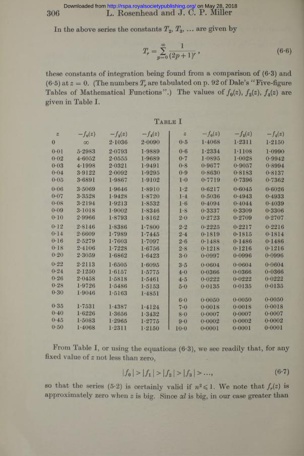
these constants of integration being found from a comparison of (6-3) and (6*5) a t 2 = 0. (The numbers Tr are tabulated on p. 92 of Dale’s “ Five-figure Tables of Mathematical Functions” .) The values of / 0(z), / 2(z), / 4(z) are given in Table I.

T a b l e Iz -/.<*> ~ fz (z ) - U z )

0 00 2-1036 2-00900-01 5-2983 2-0793 1-98890-02 4-6052 2-0555 1-96890-03 4-1998 2-0321 1-94910-04 3-9122 2-0092 1-92950-05 3-6891 1-9867 1-91020-06 3-5069 1-9646 1-89100-07 3-3528 1-9428 1-87200-08 3-2194 1-9213 1-85320-09 3-1018 1-9002 1-8346010 2-9966 1-8793 1-81620-12 2-8146 1-8386 1-78000-14 2-6609 1-7989 1-74450-16 2-5279 1-7603 1-70970-18 2-4106 1-7228 1-67560-20 2-3059 1-6862 1-64230-22 2-2113 1-6505 1-60950-24 2-1250 1-6157 1-57750-26 2-0458 1-5818 1-54610-28 1-9726 1-5486 1-51530-30 1-9046 1-5163 1-4851

0-35 1-7531 1-4387 1-41240-40 1-6226 1-3656 1-34320-45 1-5083 1-2965 1-27750-50 1-4068 1-2311 1-2150

z —-/©(*) - U z ) ~ h0-5 1-4068 1-2311 1-21500-6 1-2334 1-1108 1-09900-7 1-0895 1-0028 0-99420-8 0-9677 0-9057 0-89940-9 0-8630 0-8183 0-81371-0 0-7719 0-7396 0-73621-2 0-6217 0-6045 0-60261-4 0-5036 0-4943 0-49331-6 0-4094 0-4044 0-40391-8 0-3337 0-3309 0-33062-0 0-2723 0-2709 0-27072-2 0-2225 0-2217 0-22162-4 0-1819 0-1815 0-18142-6 0-1488 0-1486 0-14862-8 0-1218 0-1216 0-12163-0 0-0997 0-0996 0-09963-5 0-0604 0-0604 0-06044-0 0-0366 0-0366 0-03664-5 0-0222 0-0222 0-02225-0 0-0135 0-0135 0-0135

6-0 0-0050 0-0050 0-00507-0 0-0018 0-0018 0-00188-0 0-0007 0-0007 0-00079-0 0-0002 0-0002 0-0002

10-0 0-0001 0-0001 0-0001

From Table I, or using the equations (6-3), we see readily that, for any fixed value of z not less than zero,

l/o I > l/i I > |A I > I/s i > <6'7>so tha t the series (5-2) is certainly valid i f 1. We note tha t f r(z) is approximately zero when z is big. Since is big, in our case greater than




20, we see th a t near x — 0, th a t is £ = - \ccl, A - £) = fr(od + a) which isapproxim ately zero. Hence here

Vr + £) + «)•Similarly, near x = l,

( 6-8)

(6-9)

7— F o rm ulae fo r A ppr o x im a t io n

Before going on to consider a particular case, with particular numerical values of the constants, we expand P and Q in term s of powers of the small quantities n 2 and (nod)2. We substitute in (5*13) and (5-14) the series

. n£ n£00ShV2C0S^

M L M ! 84! 8!

(n£)2 (n£)6 2 ! 6 !

(7-1)

and also the values of L x and L 2 given in (5*11) and (5*12). We find, to an accuracy involving term s in n4, th a t

P = P0-n * P 2+Q = n 2Q1- . . . , (7*2)

where P0 = y0 - Y 0,

$ i = 2/2 ~ ^2 + (\cc2l2 — £ 2) Y0/ 2 !, (7 .3)

p* = y*- rt+ - >{5 - (i - g2) 5}.We note th a t Q'[ = P0, P"2 — Q1, where dashes indicate differentiation with respect to £.

Other quantities of interest are the greatest velocity and the phase- lag e, a t different values of x .We find, as far as the term in n4,

F(x) = F W + £/a) = ( P2+ W = (7*4)

e = ta n _1( —Q/P) = n2Q1/P0+ — (7-5)

If we compare (7-3) with (5-4) we see th a t

Po = fo(<xx + a) + f0{oc(l - x) + } - f 0(a) - / 0(aZ + a).

Thus, if n2is small and ad large, we have, when x < \l, the approximate relation

P = P0==f0(ocx+ a )—f 0(a), (7*6)

which is independent of od.




We may also find an approximation to Qx for the range 0 ^ < For, onconsulting Table I and equations (7'3), we see th a t — can be neglected, with an error of not more than 1 %, in comparison with the term (la 2l2-E,2)YJ2, so that, approximately,

Q = n2Qx = n \\c d — +

= n2a2x(l — x)Y0/(7-7)

The relations (7-6) and (7-7) lead to the results

F(x ) = Pq, e = \n 2 (7-8)

and, when x = 0, we find

e = — %n2alY0sinh a = — 1 (7-9)

The above considerations apply most strongly to the regions near the walls. In the central region of the fluid motion between the parallel walls, i.e. where 5<<xx<otl — 5,say, we may approximate to the various functionsby noting tha t | f 0(ax + a)\ does not exceed f % of | |. In this region| y01 is less than 2 | f 0(ocx + a)|, and T0 = almost exactly, so tha t | y0 | cannot exceed 1^ % of | Y0|. When a — 0-7 (an extreme value) and ax = 5, we find

Vo —0-007T0, (7-10)

which is the biggest ratio of y0/Y0 in our range. We still have (y2 — Y2) negligible in comparison with {\a2l2 — E>2)YJ2,so th a t in this region

P = ~ Y 0, Q = n2{\a2 (7-11)

whence F(x)= - Y 0, e = n 2(la 2l2-E,2)l2. (7*12)

The maximum value of e is thus seen to occur when 0 and is equal to

n2a2l2/8. (7-13)

Combining (7-4) and (7-11) we see th a t \ y \ , and therefore hasapproximately the constant value ( — Y0)in the central range 5 < 5,and this constant depends only on A if al is large. The value of the constant is approximately

— 0 ~fo(a)

=? loge coth \a = loge{(d + l ) / ( d - l ) } = (7-14)

Hence, using the various definitions given in § 2, we see tha t in this central




Drange the velocity is approxim ately -— which compares with4:717]

Helm holtz’s formula for the electrosmotic velocity in a field of con

stan t strength E (Helmholtz 1879; Perrin 1904).Further, the maximum phase difference, which is 8, depends only

on the non-dimensional num ber nod, and occurs a t the centre of the range.

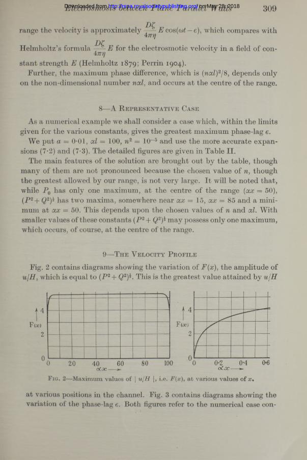
8— A R e p r e s e n t a t iv e C a s e

As a numerical example we shall consider a case which, within the limits given for the various constants, gives the greatest maximum phase-lag e.

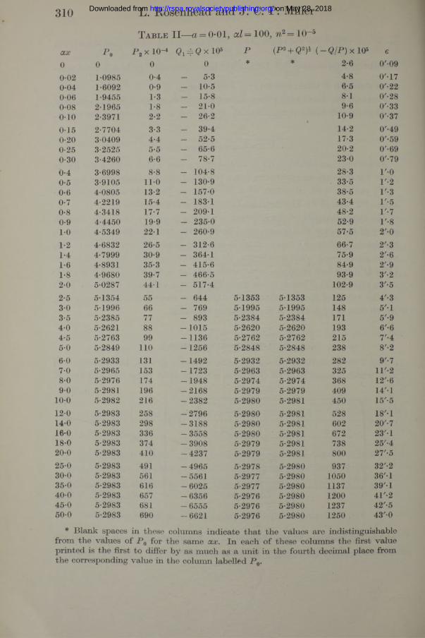
We p u t a = 0 01, od = 100, n 2 = 10-5 and use the more accurate expansions (7-2) and (7-3). The detailed figures are given in Table II .

The main features of the solution are brought out by the table, though m any of them are not pronounced because the chosen value of n, though the greatest allowed by our range, is not very large. I t will be noted tha t, while P0 has only one maximum, a t the centre of the range = 50),

(P 2 + Q2) has two maxima, somewhere near = 15, 85 and a minimum a t ax — 50. This depends upon the chosen values of n and at. W ith smaller values of these constants (P 2 + 2)* m ay possess only one maximum,which occurs, of course, a t the centre of the range.

9— T h e V e lo c ity P r o fil e

Fig. 2 contains diagrams showing the variation of F(x), the amplitude of u/H, which is equal to (P 2 + Q2)K This is the greatest value attained by u/H

» 4

F(x)2

F ig . 2—M axim um values of | u jH |, i.e. F(x), a t various values of *

a t various positions in the channel. Fig. 3 contains diagrams showing the variation of the phase-lag e. Both figures refer to the numerical case con-




T a b l e I I—a = 0 01, 100,

a x Po P 2 x 10-4 Ql == QX 105 P (P* + Q2)l ( — Q/P) x 105 e

0 0 0 0 * * 2-6 0'-09

0-02 1-0985 0-4 5-3 4-8 0'-170 0 4 1-6092 0-9 - 10-5 6-5 0'-220-06 1-9455 1-3 - 15-8 8-1 0'-280-08 2-1965 1-8 - 21-0 9-6 0'-330-10 2-3971 2-2 - 26-2

t10-9 0'-37

0 1 5 2-7704 3-3 - 39-4 14-2 0'-490-20 3-0409 4.4 - 52-5 17-3 0'-590-25 3-2525 5-5 — 65-6 20-2 0'-690-30 3-4260 6-6 - 78-7 23-0 0'-790-4 3-6998 8-8 - 104-8 28-3 l'-O0-5 3-9105 11-0 - 130-9 33-5 T -20-6 4-0805 13-2 - 157-0 38-5 T-30-7 4-2219 15-4 - 183-1 43-4 l'-50-8 4-3418 17-7 - 209-1 48-2 T-70-9 4-4450 19-9 - 235-0 52-9 l '-810 4-5349 22-1 - 260-9 57-5 2'-01-2 4-6832 26-5 - 312-6 66-7 2'-31-4 4-7999 30-9 - 364-1 75-9 2'-61-6 4-8931 35-3 - 415-6 84-9 2'-91-8 4-9680 39-7 - 466-5 93-9 3'-22 0 5-0287 44-1 - 517-4 102-9 3'-52-5 5-1354 55 - 644 5-1353 5-1353 125 4'-33 0 5-1996 66 - 769 5-1995 5-1995 148 5 '-l3-5 5-2385 77 - 893 5-2384 5-2384 171 5'-94-0 5-2621 88 -1 0 1 5 5-2620 5-2620 193 6'-64-5 5-2763 99 - 1136 5-2762 5-2762 215 7'-45-0 5-2849 110 - 1256 5-2848 5-2848 238 8'-26-0 5-2933 131 - 1492 5-2932 5-2932 282 9'-77-0 5-2965 153 -1 7 2 3 5-2963 5-2963 325 IT-28-0 5-2976 174 -1 9 4 8 5-2974 5-2974 368 12'-69-0 5-2981 196 -2 1 6 8 5-2979 5-2979 409 14 '1

10-0 5-2982 216 -2 3 8 2 5-2980 5-2981 450 15'-5120 5-2983 258 -2 7 9 6 5-2980 5-2981 528 18'-1140 5-2983 298 -3 1 8 8 5-2980 5-2981 602 20'-716-0 5-2983 336 -3 5 5 8 5-2980 5-2981 672 23'-l18-0 5-2983 374 -3 9 0 8 5-2979 5-2981 738 25'-420-0 5-2983 410 -4 2 3 7 5-2979 5-2981 800 2T-525-0 5-2983 491 -4 9 6 5 5-2978 5-2980 937 32'-230-0 5-2983 561 -5 5 6 1 5-2977 5-2980 1050 36'-135-0 5-2983 616 -6 0 2 5 5-2977 5-2980 1137 39'-l40-0 5-2983 657 -6 3 5 6 5-2976 5-2980 1200 4T-24 5 0 5-2983 681 -6 5 5 5 5-2976 5-2980 1237 42'-550-0 5-2983 690 -6 6 2 1 5-2976 5-2980 1250 43'-0

* B lank spaces in these columns ind icate th a t the values are indistinguishable from th e values of P 0 for th e sam e ax. In each of these columns th e first value p rin ted is the first to differ by as m uch as a u n it in the fourth decimal place from th e corresponding value in the colum n labelled P 0.



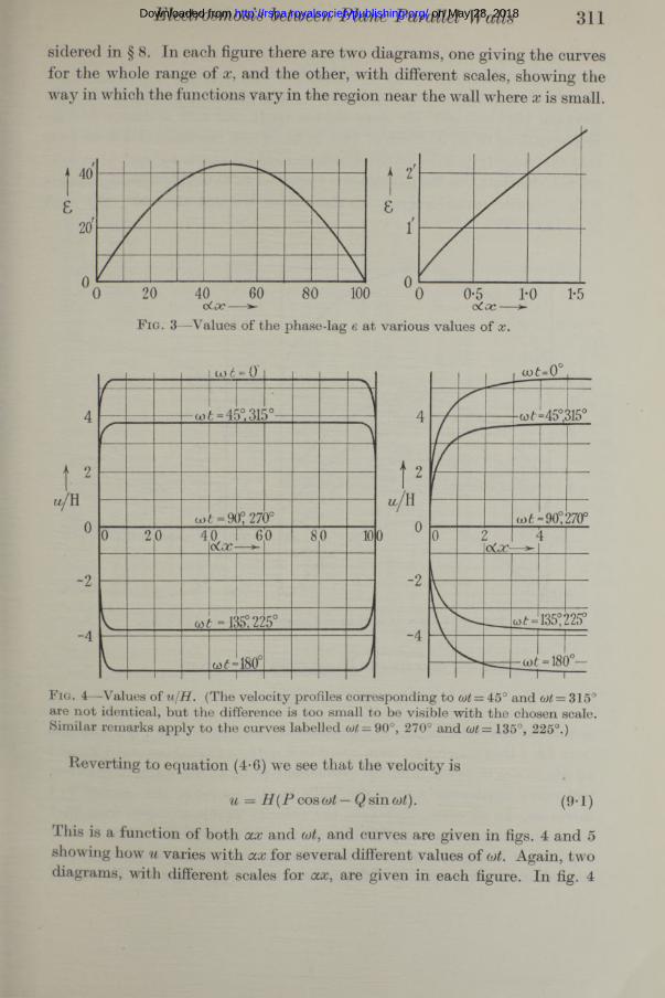
sidered in § 8. In each figure there are two diagrams, one giving the curves for the whole range of x, and the other, w ith different scales, showing the way in which the functions vary in the region near the wall where x is small.


F ig . 3— V alues of th e phase-lag e a t various values o f x .

4

-4

F ig . 4— Values of ujH . (The velocity profiles corresponding to cot — 45° an d 315° are n o t identical, b u t th e difference is too sm all to be visible w ith th e chosen scale. S im ilar rem arks app ly to th e curves labelled cot = 90°, 270° an d 135°, 225°.)

Reverting to equation (4-6) we see th a t the velocity is

u = H (P coscot—Q sin cot). (9-1)

This is a function of both ax and cot, and curves are given in figs. 4 and 5 showing how u varies with ax for several different values of cot. Again, two diagrams, with different scales for ax, are given in each figure. In fig. 4




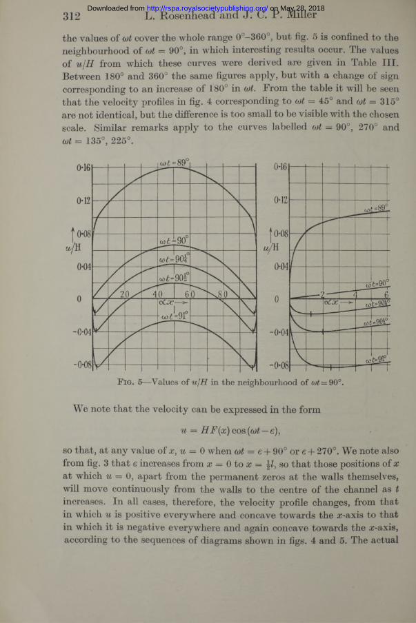
the values of cot cover the whole range 0°—360°, but fig. 5 is confined to the neighbourhood of cot = 90°, in which interesting results occur. The values of ulH from which these curves were derived are given in Table III. Between 180° and 360° the same figures apply, but with a change of sign corresponding to an increase of 180° in cot. From the table it will be seen th a t the velocity profiles in fig. 4 corresponding to o)t = 45° and 315° are not identical, but the difference is too small to be visible with the chosen scale. Similar remarks apply to the curves labelled cot = 90°, 270° and cot = 135°, 225°.

F ig . 5—Values of u jH in th e neighbourhood of 0)t = 90°.

We note tha t the velocity can be expressed in the form

u = HF(x) cos (cot —e),

so that, at any value of x, u = 0 when cot = e + 90° or e + 270°. We note also from fig. 3 th a t e increases from x = 0 to x so th a t those positions of x a t which u = 0, apart from the permanent zeros a t the walls themselves, will move continuously from the walls to the centre of the channel as t increases. In all cases, therefore, the velocity profile changes, from that in which u is positive everywhere and concave towards the ir-axis to tha t in which it is negative everywhere and again concave towards the x-axis, according to the sequences of diagrams shown in figs. 4 and 5. The actual



changes during the beginning of th a t period of transition during which cot passes through the value 90° are shown in fig. 5. There is a similar set of figures corresponding to cot = 270°, bu t these are not shown.


T a b l e I I I — V a l u e s o f u/H a t v a r io u s T im e s d u r in g a H a l f -c y c l e

a = 0-01, al= 100,ax cot = 0° 45° 89° 90°

Oo05 90Jo 91° 135°0 0 0 0 0 0 0 0 001 2-40 1-70 0-042 0-000 - 0-010 - 0-021 -0 -0 4 1 - 1 -7 00-2 3 0 4 2-15 0-054 0-001 -0 -0 1 3 -0 -0 2 6 -0 -0 5 3 -2 -1 50-3 3-43 2-42 0-061 0-001 -0 -0 1 4 -0 -0 2 9 -0 -0 5 9 -2 -4 20-4 3-70 2-62 0-066 0-001 -0 -0 1 5 - 0-031 - 0-064 -2 -6 20-6 4-08 2-89 0-073 0-002 -0 -0 1 6 - 0-034 -0 -0 7 0 - 2-880-8 4-34 3-07 0-078 0-002 - 0-017 -0 -0 3 6 -0 -0 7 4 -3 -0 710 4-53 3-21 0-082 0-003 -0 -0 1 7 -0 -0 3 7 -0 -0 7 7 - 3 -2 01-5 4-85 3-43 0-089 0-004 -0 -0 1 7 -0 -0 3 8 -0 -0 8 1 -3 -4 32 0 5 0 3 3-56 0-093 0-005 - 0 0 1 7 -0 -0 3 9 -0 -0 8 3 -3 -5 53 0 5-200 3-682 0-099 0-008 -0 -0 1 5 -0 -0 3 8 -0 -0 8 3 -3 -6 7 14-0 5-262 3-728 0-102 0-010 -0 -0 1 3 -0 -0 3 6 -0 -0 8 2 -3 -7 1 45-0 5-285 3-746 0-105 0-013 - 0-010 - 0-034 -0 -0 8 0 -3 -7 2 86 0 5-293 3-753 0-107 0-015 -0 -0 0 8 - 0-031 -0 -0 7 8 -3 -7 3 27-0 5-296 3-757 0-110 0-017 -0 -0 0 6 -0 -0 2 9 -0 -0 7 5 -3 -7 3 38-0 5-2974 3-760 0-112 0-019 -0 -0 0 4 -0 -0 2 7 -0 -0 7 3 -3 -7 3 29 0 5-2979 3-761 0-114 0-022 - 0-001 -0 -0 2 4 -0 -0 7 1 -3 -7 3 1

10-0 5-2980 3-763 0-116 0-024 + 0-001 - 0-022 -0 -0 6 9 -3 -7 2 915 0 5-2980 3-770 0-126 0-034 + 0-011 - 0-012 -0 -0 5 9 -3 -7 2 220-0 5-2979 3-776 0-135 0-042 + 0-019 -0 -0 0 4 -0 -0 5 0 -3 -7 1 630-0 5-2977 3-785 0-148 0-056 + 0-032 + 0-009 - 0-037 -3 -7 0 74 0 0 5-2976 3-791 0-156 0-064 + 0-040 + 0-017 -0 -0 2 9 -3 -7 0 150-0 5-2976 3-793 0-159 0-066 + 0-043 + 0-020 -0 -0 2 6 -3 -6 9 9

W ith our choice of the constants, the velocity profile with three stationary values, of the type shown in fig. 5 , cot = 91°, persists for about a quarter of the complete cycle, but w ith smaller values of n and ocl this period can be considerably reduced, even to a fraction of a degree. The magnitude of the dip in the velocity profile in the centre of the channel is never greater than 1 % of the maximum velocity attained there, and may be much less. This is below the limits of experimental error a t present available and therefore may not have been observed.

10— S u m m a r y o f t h e P r in c ip a l R e s u l t s

1—The equation satisfied by the fluid flow is

dudi

dhidx2

QeiojiF2Aea c{A2e2ocx + 1} 2 A ea(l~x){A 2e2a(l~x) + 1}“|{A2e2ax - Ip H 2g2a(Z—x) — lj2




The velocity, which is restricted to be zero a t the walls, is the real part of u obtained from this equation.

2—When the field strength is E cos cot, the velocity of the fluid is

HF(x ) cos( — e) ,

where F(x) — P0 — ni (P0P2 — ^Ql)/Po+

and e = vPQJPq + ...,

which is also a function of x. In these expressions

Po = V o -Y0’Qi = y z - Y* + { W P -I? )Y J 2 \ ,

P2 = y i - Y i + (1 - f 2) { 5 - (f - £2) .

The values of y0, y2, yi and T0, Y2, T4 are obtained from Table I. The curveshowing the variation of velocity along a line perpendicular to the walls is always symmetrical with respect to the walls.

3—The highest value of u obtaining a t any point is given by the equation u = HF(x), (cf. fig. 2 and Table II). I f is small, u = H(y0 — 1^), and in the central region 5 <ax<od — 5,

u= - H Y 0 = H loge{(A + 1 )/(A - 1)} =

DCIn the central region the velocity is approximately E cos which

DCshould be compared with Helmholtz’s formula - — E for the velocity in

a field of constant strength E.

4— The phase difference e increases continuously from the value/f 2_ 1 A i 1

— \n 2odY0sinh a = \n 2cd — -— loge — -jOL — 1

at the walls to the value n2<x2l2/8 a t points half-way between the walls. Except near the walls, we have e= \n 2<x2x(l — x), (cf. fig. 3 and Table II).

5— The curves showing the form of the velocity profile a t various times during one cycle of the alternating current are shown in figs. 4 and 5. Although these curves refer to one set of values of the physical constants, they are characteristic of the whole range considered. I t therefore appears




th a t if the distance between the walls is of the order of m agnitude which allows of a m easurement of the surface conductivity (or of the electrosmotic velocity in the alternating field), th a t is if the Gouy theory can be applied, then the normal phenomena of electrosmosis exist, even with frequencies of the alternating current as high as 105/sec. For two periods during a complete cycle, the velocity profile shows a dip in the middle portion. This dip may persist for a quarter-cycle a t a time or for a very much shorter period, depending on the chosen values of the constants. The magnitude of the dip is never greater than 1 % of the greatest velocity attained in the centre of the channel, and may be much less. This is below the limits of error associated w ith the present experimental technique, and this phenomenon therefore may not have been observed.

N o t e b y J . J . B ik e r m a n

Electrokinetic phenomena represent the best, indeed almost the only, source of information concerning the potential difference between the surface and the body of a liquid.

Unfortunately, in the first approximation used by Helmholtz, the electrokinetic potential £ can only be calculated with an uncertain multiplier. Thus Helmholtz believed £ to be of the order of 5 V, whilst modern workers (Perrin 1904) accept values of £less than OT V. I t is even possible (in the first approximation) to account for the simplest electrokinetic phenomena without using a definite value of £ a t all. On the other hand, the formulae of Helmholtz are independent of the structure of the surface charge.

The situation changes when the second approximation of the theory is considered or effects of the second order are examined: (a) the value of £ becomes unambiguous, and (6) the equations depend on the assumed structure of the surface charge. Dealing with the second order phenomena it is possible and convenient to use the surface conductivity as the fundamental property. This is the reason for its importance (Bikerman 1935). Electrosmosis is an effect of the first order, and only the second approximation of its theory depends on the assumed structure of the double layer; on the other hand, the surface conductivity is an effect of the second order and cannot be accounted for Avithout an assumption concerning the structure of the double layer.

The surface conductivity has a twofold origin: (a) the surface layer of the liquid contains a different number of ions per cubic centimetre from the liquid in bulk, and (6) the surface layer of the liquid contains different numbers




of positive and negative ions; it is charged so th a t its electrosmotic movement produces an electric current. In agreement with this the mathematical expression for the surface conductivity contains two terms. I t was suggested (Bikerman 1933) tha t both terms depend upon the frequency of the alternating current used for measuring the surface conductivity, but in different ways. The first one is a simple concentration term and should show a “ dispersion” a t the same frequencies as the ordinary conductivity, tha t is, a t about 107 cycles/sec. (By the “ dispersion” of a quantity we mean the variation of the quantity considered with the frequency of the alternating current.) The second term presupposes the existence of a regular movement of the whole liquid and would, therefore, disappear a t some lower frequencies. A consequence of this theory is th a t the magnitudes of both these terms are of the same order under the usual conditions, and, as a result, the values of the surface conductivity should fall, with rising frequency, to about one-half of their values for direct current. The exact knowledge of the dispersion of surface conductivity, th a t is, the extent of the fall and the frequency interval where it occurs, would be, for the science of electrokinetics, as useful as the discovery and investigation of the dispersion of ordinary conductivity was for the science of electrolytes (Debye and Falkenhagen 1928).

As far as experimental evidence is concerned (Urban, Feldman and White 1935) no difference has been noticed between the surface conductivity for direct current and 1000 cycles alternating current, and more extensive measurements have been planned both in England and in the U.S.A. In order to compare experimental evidence with theory it is necessary to calculate the critical interval of frequencies. Professor Rosenhead and Dr. Miller were kind enough to carry out investigations along these lines. They came to the unexpected conclusion th a t the dispersion of electrosmosis is not in evidence even a t frequencies as high as 105 cycles/sec. This suggests th a t the dispersion of electrosmosis, if it occurs a t all, occurs a t frequencies a t least as high as those which produce the Debye-Falkenhagen effect (107 cycles/sec.). Hence many im portant consequences follow, of which three may be mentioned here:

(1) The suggested checking of the theory of surface conductivity by measuring its dispersion is impracticable.

(2) The comparison (Abramson 1934) of the experimental results observed a t various frequencies, with the formula for surface conductivity, taking both terms in the formula into consideration, is justified.

(3) The discrepancy between the surface conductivity values found by different observers cannot be attributed to the difference of the frequencies used.




R e f e r e n c e s

Abram son 1934 “ Electrokinetic Phenom ena.” New York, U.S.A. B ikerm an 1933 phys. Chem. A, 163 , 378.

— 1935 Kolloidzschr. 72, 100.Debye and Falkenhagen 1928 Phys. 29, 401.Gouy 1910 J . Phys. Radium , (4), 9, 457.Helm holtz 1879 A nn . Phys., Lpz., 7, 337.Perrin 1904 J . Chim. phys. 2, 601.U rban, Feldm an and W hite 1935 J • Phys. Chem. 39, 605.



Electrosmosis between plane parallel walls...

Documents

Transcript of Electrosmosis between plane parallel walls...