Theevolutionofairresonance...
26
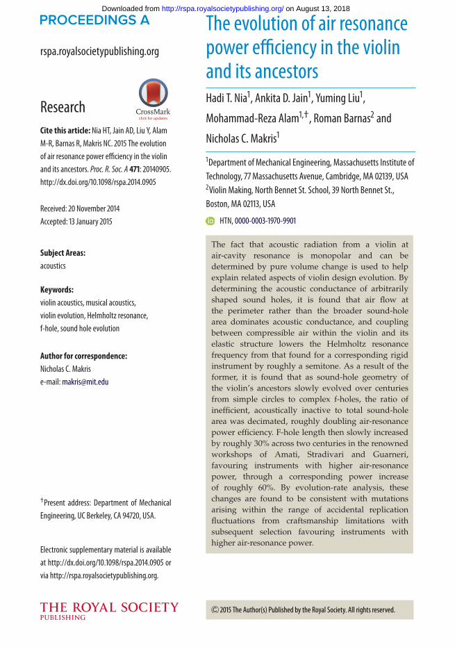
rspa.royalsocietypublishing.org Research Cite this article: Nia HT, Jain AD, Liu Y, Alam M-R, Barnas R, Makris NC. 2015 The evolution of air resonance power efficiency in the violin and its ancestors. Proc. R. Soc. A 471: 20140905. http://dx.doi.org/10.1098/rspa.2014.0905 Received: 20 November 2014 Accepted: 13 January 2015 Subject Areas: acoustics Keywords: violin acoustics, musical acoustics, violin evolution, Helmholtz resonance, f-hole, sound hole evolution Author for correspondence: Nicholas C. Makris e-mail: [email protected] † Present address: Department of Mechanical Engineering, UC Berkeley, CA 94720, USA. Electronic supplementary material is available at http://dx.doi.org/10.1098/rspa.2014.0905 or via http://rspa.royalsocietypublishing.org. The evolution of air resonance power efficiency in the violin and its ancestors Hadi T. Nia 1 , Ankita D. Jain 1 , Yuming Liu 1 , Mohammad-Reza Alam 1,† , Roman Barnas 2 and Nicholas C. Makris 1 1 Department of Mechanical Engineering, Massachusetts Institute of Technology, 77 Massachusetts Avenue, Cambridge, MA 02139, USA 2 Violin Making, North Bennet St. School, 39 North Bennet St., Boston, MA 02113, USA HTN, 0000-0003-1970-9901 The fact that acoustic radiation from a violin at air-cavity resonance is monopolar and can be determined by pure volume change is used to help explain related aspects of violin design evolution. By determining the acoustic conductance of arbitrarily shaped sound holes, it is found that air flow at the perimeter rather than the broader sound-hole area dominates acoustic conductance, and coupling between compressible air within the violin and its elastic structure lowers the Helmholtz resonance frequency from that found for a corresponding rigid instrument by roughly a semitone. As a result of the former, it is found that as sound-hole geometry of the violin’s ancestors slowly evolved over centuries from simple circles to complex f-holes, the ratio of inefficient, acoustically inactive to total sound-hole area was decimated, roughly doubling air-resonance power efficiency. F-hole length then slowly increased by roughly 30% across two centuries in the renowned workshops of Amati, Stradivari and Guarneri, favouring instruments with higher air-resonance power, through a corresponding power increase of roughly 60%. By evolution-rate analysis, these changes are found to be consistent with mutations arising within the range of accidental replication fluctuations from craftsmanship limitations with subsequent selection favouring instruments with higher air-resonance power. 2015 The Author(s) Published by the Royal Society. All rights reserved. on August 13, 2018 http://rspa.royalsocietypublishing.org/ Downloaded from
Transcript of Theevolutionofairresonance...
rspa.royalsocietypublishing.org
ResearchCite this article: Nia HT, Jain AD, Liu Y, AlamM-R, Barnas R, Makris NC. 2015 The evolutionof air resonance power efficiency in the violinand its ancestors. Proc. R. Soc. A 471: 20140905.http://dx.doi.org/10.1098/rspa.2014.0905
Received: 20 November 2014Accepted: 13 January 2015
Subject Areas:acoustics
Keywords:violin acoustics, musical acoustics,violin evolution, Helmholtz resonance,f-hole, sound hole evolution
Author for correspondence:Nicholas C. Makrise-mail: [email protected]
†Present address: Department of MechanicalEngineering, UC Berkeley, CA 94720, USA.
Electronic supplementary material is availableat http://dx.doi.org/10.1098/rspa.2014.0905 orvia http://rspa.royalsocietypublishing.org.
The evolution of air resonancepower efficiency in the violinand its ancestorsHadi T. Nia1, Ankita D. Jain1, Yuming Liu1,
Mohammad-Reza Alam1,†, Roman Barnas2 and
Nicholas C. Makris1
1Department of Mechanical Engineering, Massachusetts Institute ofTechnology, 77 Massachusetts Avenue, Cambridge, MA 02139, USA2Violin Making, North Bennet St. School, 39 North Bennet St.,Boston, MA 02113, USA
HTN, 0000-0003-1970-9901
The fact that acoustic radiation from a violin atair-cavity resonance is monopolar and can bedetermined by pure volume change is used to helpexplain related aspects of violin design evolution. Bydetermining the acoustic conductance of arbitrarilyshaped sound holes, it is found that air flow atthe perimeter rather than the broader sound-holearea dominates acoustic conductance, and couplingbetween compressible air within the violin and itselastic structure lowers the Helmholtz resonancefrequency from that found for a corresponding rigidinstrument by roughly a semitone. As a result of theformer, it is found that as sound-hole geometry ofthe violin’s ancestors slowly evolved over centuriesfrom simple circles to complex f-holes, the ratio ofinefficient, acoustically inactive to total sound-holearea was decimated, roughly doubling air-resonancepower efficiency. F-hole length then slowly increasedby roughly 30% across two centuries in the renownedworkshops of Amati, Stradivari and Guarneri,favouring instruments with higher air-resonancepower, through a corresponding power increaseof roughly 60%. By evolution-rate analysis, thesechanges are found to be consistent with mutationsarising within the range of accidental replicationfluctuations from craftsmanship limitations withsubsequent selection favouring instruments withhigher air-resonance power.
2015 The Author(s) Published by the Royal Society. All rights reserved.
on August 13, 2018http://rspa.royalsocietypublishing.org/Downloaded from
2
rspa.royalsocietypublishing.orgProc.R.Soc.A471:20140905
...................................................
1. IntroductionAcoustic radiation from a violin at its lowest frequency resonance is monopolar [1] and can bedetermined by pure volume change [2–4]. We use this to help explain certain aspects of violindesign evolution that are important to acoustic radiation at its lowest frequency resonance. Thislowest frequency resonance is also known as air cavity resonance and Helmholtz resonance [3–5]. Air cavity resonance has been empirically identified as an important quality discriminatorbetween violins [6–8] and is functionally important because it amplifies the lower frequency rangeof a violin’s register [7–9]. It corresponds to the violin’s lowest dominant mode of vibration. Sincemost of the violin’s volume is devoted to housing the air cavity, the air cavity has an importanteffect on a violin’s acoustic performance at low frequencies by coupling interior compressible airwith the violin’s elastic structure and air flow to the exterior via sound holes.
Owing to its long-standing prominence in world culture, we find enough archaeologicaldata exist for the violin and its ancestors to quantitatively trace design traits affecting radiatedacoustic power at air cavity resonance across many centuries of previously unexplained change.By combining archaeological data with physical analysis, it is found that as sound hole geometryof the violin’s ancestors slowly evolved over a period of centuries from simple circular openingsof tenth century medieval fitheles to complex f-holes that characterize classical seventeenth–eighteenth century Cremonese violins of the Baroque period, the ratio of inefficient, acousticallyinactive to total sound hole area was decimated, making air resonance power efficiency roughlydouble. Our findings are also consistent with an increasing trend in radiated air resonance powerhaving occurred over the classical Cremonese period from roughly 1550 (the Late Renaissance) to1750 (the Late Baroque Period), primarily due to corresponding increases in f-hole length. This isbased upon time series of f-hole length and other parameters that have an at least or nearly first-order effect on temporal changes in radiated acoustic power at air cavity resonance. The timeseries are constructed from measurements of 470 classical Cremonese violins made by the masterviolin-making families of Amati, Stradivari and Guarneri. By evolution rate analysis, we findthese changes to be consistent with mutations arising within the range of accidental replicationfluctuations from craftsmanship limitations and selection favouring instruments with higherair-resonance power, rather than drastic preconceived design changes. Unsuccessful nineteenthcentury mutations after the Cremonese period known to be due to radical design preconceptionsare correctly identified by evolution rate analysis as being inconsistent with accidental replicationfluctuations from craftsmanship limitations and are quantitatively found to be less fit in terms ofair resonance power efficiency.
Measurements have shown that acoustic radiation from the violin is omni-directional at the aircavity resonance frequency [1]. These findings are consistent with the fact that the violin radiatessound as an acoustically compact, monopolar source [2–4], where dimensions are much smallerthan the acoustic wavelength, at air resonance. The total acoustic field radiated from a monopolesource can be completely determined from temporal changes in air volume flow from the source[2–4,10,11]. For the violin, the total volume flux is the sum of the air volume flux through thesound hole and the volume flux of the violin structure. Accurate estimation of monopole radiationat air resonance then only requires accurate estimation of volume flow changes [2,3,11,12] ratherthan more complicated shape changes of the violin [8,9,13] that do not significantly affect thetotal volume flux. By modal principles, such other shape changes may impact higher frequencyacoustic radiation from the violin. Structural modes describing shape changes at and near airresonance have been empirically related to measured radiation, where modes not leading tosignificant net volume flux, such as torsional modes, have been found to lead to insignificantradiation [8,13]. Since acoustic radiation from the violin at air resonance is monopolar [1], andso can be determined from changes in total volume flow over time, a relatively simple and clearmathematical formulation for this radiation is possible by physically estimating the total volumeflux resulting from the corresponding violin motions that have been empirically shown [13] tolead to the dominant radiation at air resonance.
Here we isolate the effect of sound hole geometry on acoustic radiation at air resonance bydeveloping a theory for the acoustic conductance of arbitrarily shaped sound holes. We use this
on August 13, 2018http://rspa.royalsocietypublishing.org/Downloaded from
3
rspa.royalsocietypublishing.orgProc.R.Soc.A471:20140905
...................................................
to determine limiting case changes in radiated acoustic power over time for the violin and itsancestors due to sound-hole change alone. These limiting cases are extremely useful because theyhave exact solutions that are only dependent on the simple geometric parameters of sound holeshape and size, as they varied over time, and are not dependent on complex elastic parameters ofthe violin. We then estimate monopole radiation from the violin and its ancestors at air resonancefrom elastic volume flux analysis. This elastic volume flux analysis leads to expected radiatedpower changes at air resonance that fall between and follow a similar temporal trend as thoseof the geometric limiting cases. The exact solution from rigid instrument analysis leads to asimilar air resonance frequency temporal trend as elastic analysis but with an offset in frequencyfrom measured values by roughly a semitone. Elastic volume flux estimation, on the other hand,matches measured air resonance frequencies of extant classical Cremonese instruments to roughlywithin a quarter of a semitone or a Pythagorean comma [14]. This indicates that rigid analysis maynot be sufficient for some fine-tuned musical applications.
While Helmholtz resonance theory for rigid vessels [3–5] has been experimentally verifiedfor simple cavity shapes and elliptical or simple circular sound holes (e.g. [15–18]) as in theguitar, it has not been previously verified for the violin due to lack of a model for the acousticconductance of the f-hole. Parameter fit and network analogy approaches to violin modelling[19], rather than fundamental physical formulations that have been developed for the violin andrelated instruments [5,9,20,21], have led to results inconsistent with classical Helmholtz resonancetheory [3–5] even for rigid vessels. Here it is found both experimentally and theoretically thatwhen violin plates are rigidly clamped, the air-cavity resonance frequency still follows the classicrigid body dependence on cavity volume and sound hole conductance of Helmholtz resonatortheory [3–5]. It is also found that when the plate clamps are removed, air-cavity resonancefrequency is reduced by a percentage predicted by elastic volume flux analysis, roughly asemitone. Discussions on the dependence of air resonance frequency, and consequently acousticconductance, on sound hole geometry have typically focused on variations in sound hole area(e.g. [22–25]). The fluid-dynamic theory developed here shows that the conductance of arbitrarilyshaped sound holes is in fact proportional to the sound hole perimeter length and not the area.This is verified by theoretical proof, experimental measurement and numerical computation. Thisperimeter dependence is found to be of critical importance in explaining the physics of air-flowthrough f-holes and sound radiation from a violin at air resonance. It is also found to havesignificantly impacted violin evolution.
2. Determining the acoustic conductance of arbitrarily shaped sound holesSound hole conductance C [3,4] is related to air volume flow through the sound hole by
mair(t) = C�P(t), (2.1)
where �P(t) is the pressure difference across the hole-bearing wall, for monopolar sound sources[2–4] like the violin at the air resonance frequency, and mair(t) is mass flow rate through thesound hole [2], which is the product of air volume flow rate and air density, at time t. Theacoustic pressure field radiated from a sound hole of dimensions much smaller than the acousticwavelength is proportional to the mass flow rate’s temporal derivative [2–4], and consequentlythe temporal derivative of the air volume flow rate and conductance via equation (2.1). Analyticsolutions for conductance exist for the special cases of circular and elliptical sound holes [3,4],where conductance equals diameter in the former, but are not available for general soundhole shapes.
A theoretical method for determining the acoustic conductance of an arbitrarily shapedsound hole is described here. Acoustic conductance is determined by solving a mixed boundaryvalue problem [2–4,26] for approximately incompressible fluid flow through a sound hole.This approach is used to theoretically prove that conductance is approximately the product ofsound hole perimeter length L and a dimensionless shape factor α in §3. It is then numerically
on August 13, 2018http://rspa.royalsocietypublishing.org/Downloaded from
4
rspa.royalsocietypublishing.orgProc.R.Soc.A471:20140905
...................................................
implemented in §§4 and 5 to quantitatively analyse the evolution of violin power efficiency at airresonance. It is experimentally verified for various sound hole shapes, including the violin f-hole,in §§4, 5 and 7. The approach described here is for sound hole dimensions small compared withthe acoustic wavelength, as is typical at the air resonance frequency of many musical instruments,including those in the violin, lute, guitar, harp and harpsichord families.
Assuming irrotational fluid flow with velocity potential φ(x, y, z), the boundary value problem[2–4,26] is to solve Laplace’s equation in the upper half plane above a horizontal wall with theboundary conditions that (i) φ = 1 over the sound hole aperture in the wall, (ii) ∂φ/∂n = 0 on thewall, corresponding to zero normal velocity, and (iii) φ vanishes as the distance from the openingapproaches infinity. The normal fluid flow velocity through the sound hole is
un = ∂φ
∂n(2.2)
and the conductance C is
C = 12
∫∫S
un dS, (2.3)
where S is the sound hole area. From the boundary integral formulation [27], we develop arobust boundary element method to solve the stated boundary value problem for φ and obtainthe exact solution for the normal velocity un(x, y, z) on the opening from which conductance isthen determined [3,4]. This method is found to be effective for arbitrary sound hole shapes andmultiple sound holes. In the limit as the separation between multiple sound holes approachesinfinity, the total conductance equals the sum of the conductances of the individual sound holes.When the separation between sound holes is small, the total conductance is smaller than the sumof the conductances of individual sound holes. For typical Cremonese violins, the conductancetheory developed here shows that the interaction of two f-holes reduces the total conductance byroughly 7% from the sum of conductances of individual f-holes. This leads to a roughly 4% changein air resonance frequency, which is a significant fraction of a semitone, and a roughly 15% changein radiated acoustic power at air resonance. The conductance formulation of equation (2.3) is forwall thickness, hsh, asymptotically small near the sound hole, hsh � L, which is generally the casefor the violin and its ancestors as well as guitars, lutes and many other instruments. The effect offinite wall thickness on C can be included by use of Rayleigh’s formulation [3], which becomesnegligible for sufficiently thin wall thickness at the sound hole.
For the special case of an ellipse, both perimeter length [28] and Rayleigh’s analytic solutionfor the conductance of an ellipse [3] are directly proportional to the ellipse’s major radius, andso are proportional to each other for a fixed eccentricity. In the elliptical case, for example,the eccentricity determines the constant of proportionality, i.e. the shape factor α, between theconductance and the perimeter length. With only the ellipse solution available, Rayleigh observedthat sound hole conductance ‘C varies as the linear dimension’ [3] of the sound hole, but he didnot supply a general proof or describe the physical mechanisms leading to this dimensionality.
3. Theoretical proof of the linear proportionality of conductance on sound holeperimeter length
Here the conductance of a sound hole is proved to be linearly proportional to sound holeperimeter length for L � hsh. Total sound hole area S in equation (2.3) can be subdivided intoN elemental areas sj, which share a common vertex inside S, such that the total sound holeconductance from equation (2.3) is
C = 12
N∑j=1
∫∫sj
un(x, y) dS, (3.1)
on August 13, 2018http://rspa.royalsocietypublishing.org/Downloaded from
5
rspa.royalsocietypublishing.orgProc.R.Soc.A471:20140905
...................................................
where S = ∑Nj=1 sj, with sj containing a piece-wise smooth boundary element lj of the sound hole
perimeter. Using Stokes theorem, the integral in equation (3.1) can be written as∫∫
sj
un(x, y) dS =∮
Lj
A dx + B dy, (3.2)
where Lj is the total boundary contour of the elemental area sj and ∂B/∂x − ∂A/∂y = un(x, y).The boundary value problem for φ(x, y, z) has a special feature that un(x, y, z) has a weak,
integrable singularity at the perimeter of the sound hole. A local coordinate system (x′, y′) with x′along lj and y′ = 0 can be defined on lj so that equation (3.2) reduces to
∫∫sj
un(x, y) dS =∫
ljA′ dx′ +
∫�lj
A′ dx′ + B′ dy′, (3.3)
where Lj = lj + �lj, ∂B′/∂x′ − ∂A′/∂y′ = un(y′) and un(y′) = a(y′)β from the three-dimensionalcorner flow solution [29] with −0.5 < β < 0. Then A′ = b + (a/(β + 1))(y′)β+1 with B′ = 0 or anarbitrary constant is a solution to ∂B′/∂x′ − ∂A′/∂y′ = un(y′), and so
∫lj A′ dx′ = blj where a and
b are constants.Then, from equations (3.1) and (3.3)
C = 12
N∑j=1
blj + 12
N∑j=1
∫�lj
A′ dx′ + B′ dy′
︸ ︷︷ ︸=0
, (3.4)
where the second term vanishes since the total contribution from the edges of sj other than ljcancel out from Stokes theorem. Then, the conductance C of the sound hole
C = 12 bL = αL (3.5)
is proportional to the sound hole perimeter length L, b depends on the shape of the sound holeand α = b/2 is the shape factor.
4. Evolution of sound hole shape from the tenth to the eighteenth centuriesand its effect on radiated air resonance power of the violin and its europeanancestors
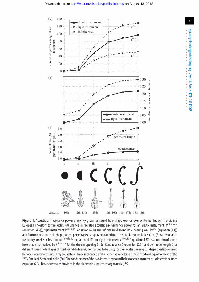
Upper and lower limiting cases are determined by exact solutions for the changes in radiatedacoustic power over time due solely to changes in the purely geometric parameter of sound holeshape for the violin and its ancestors (figure 1a, electronic supplementary material, §§1 and 2).These are compared with the radiated power changes over time at air resonance from elasticvolume flux analysis (§9 and electronic supplementary material, §§3 and 4) (figure 1a). To isolatethe effect of sound hole geometry in figure 1a–c, all cases have constant forcing amplitude overtime, are normalized to the circular sound hole case, and have all other parameters includingsound-hole area and air cavity volume fixed over time. So, the basic question is, for the samearea of material cut from an instrument to make a sound hole, what is the isolated effect of theshape of this sound hole on the air resonance frequency and the acoustic power radiated at thisresonance frequency?
The upper limiting case corresponds to the radiated power change of an infinite rigid soundhole bearing wall, where the exact analytical solution for total power in a frequency band �f isgiven by
Wwall = 1T
∫�f
|�P( f )|2πρaircair
df C2 (4.1)
on August 13, 2018http://rspa.royalsocietypublishing.org/Downloaded from
6
rspa.royalsocietypublishing.orgProc.R.Soc.A471:20140905
...................................................
140elastic instrument
rigid instrument
infinite wall
C1
C1.7
C2120
100
80
60
40
% r
adia
ted
pow
er c
hang
e at
air
re
sona
nce
20
1.30
1.25
1.20
1.15
1.10
1.05
1.00 norm
aliz
ed a
ir r
eson
ance
fre
quen
cy
0
(a)
(b)
(c)
elastic instrument
rigid instrument
perimeter length
3.0
2.6
2.2
1.8
cond
ucta
nce
(C)
peri
met
er le
ngth
(L
)
1.4
1.0
i ii
century: 10th 12th–13th 15th–16th 16th–17th 16th–18th
iii iv v vi
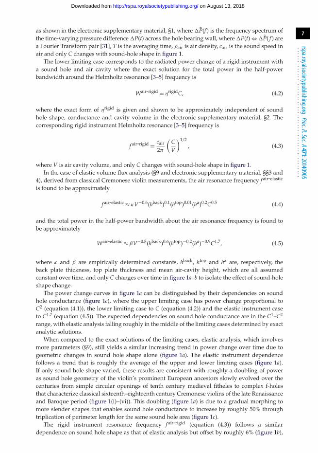
conductance
13th
Figure 1. Acoustic air-resonance power efficiency grows as sound hole shape evolves over centuries through the violin’sEuropean ancestors to the violin. (a) Change in radiated acoustic air-resonance power for an elastic instrument Wair-elastic
(equation (4.5)), rigid instrument Wair-rigid (equation (4.2)) and infinite rigid sound hole bearing wall Wwall (equation (4.1))as a function of sound hole shape, where percentage change is measured from the circular sound hole shape. (b) Air-resonancefrequency for elastic instrument f air-elastic (equation (4.4)) and rigid instrument f air-rigid (equation (4.3)) as a function of soundhole shape, normalized by f air-elastic for the circular opening (i). (c) Conductance C (equation (2.3)) and perimeter length L fordifferent sound hole shapes of fixed sound-hole area, normalized to be unity for the circular opening (i). Shape overlap occurredbetween nearby centuries. Only sound hole shape is changed and all other parameters are held fixed and equal to those of the1703 ‘Emiliani’ Stradivari violin [30]. The conductance of the two interacting sound holes for each instrument is determined fromequation (2.3). Data sources are provided in the electronic supplementary material, §5.
on August 13, 2018http://rspa.royalsocietypublishing.org/Downloaded from
7
rspa.royalsocietypublishing.orgProc.R.Soc.A471:20140905
...................................................
as shown in the electronic supplementary material, §1, where �P(f ) is the frequency spectrum ofthe time-varying pressure difference �P(t) across the hole bearing wall, where �P(t) ⇔ �P( f ) area Fourier Transform pair [31], T is the averaging time, ρair is air density, cair is the sound speed inair and only C changes with sound-hole shape in figure 1.
The lower limiting case corresponds to the radiated power change of a rigid instrument witha sound hole and air cavity where the exact solution for the total power in the half-powerbandwidth around the Helmholtz resonance [3–5] frequency is
Wair-rigid = ηrigidC, (4.2)
where the exact form of ηrigid is given and shown to be approximately independent of soundhole shape, conductance and cavity volume in the electronic supplementary material, §2. Thecorresponding rigid instrument Helmholtz resonance [3–5] frequency is
f air-rigid = cair
2π
(CV
)1/2, (4.3)
where V is air cavity volume, and only C changes with sound-hole shape in figure 1.In the case of elastic volume flux analysis (§9 and electronic supplementary material, §§3 and
4), derived from classical Cremonese violin measurements, the air resonance frequency f air-elastic
is found to be approximately
f air-elastic ≈ κV−0.6(hback)0.1(htop)0.01(ha)0.2C0.5 (4.4)
and the total power in the half-power bandwidth about the air resonance frequency is found tobe approximately
Wair-elastic ≈ βV−0.8(hback)0.6(htop)−0.2(ha)−0.9C1.7, (4.5)
where κ and β are empirically determined constants, hback, htop and ha are, respectively, theback plate thickness, top plate thickness and mean air-cavity height, which are all assumedconstant over time, and only C changes over time in figure 1a–b to isolate the effect of sound-holeshape change.
The power change curves in figure 1a can be distinguished by their dependencies on soundhole conductance (figure 1c), where the upper limiting case has power change proportional toC2 (equation (4.1)), the lower limiting case to C (equation (4.2)) and the elastic instrument caseto C1.7 (equation (4.5)). The expected dependencies on sound hole conductance are in the C1–C2
range, with elastic analysis falling roughly in the middle of the limiting cases determined by exactanalytic solutions.
When compared to the exact solutions of the limiting cases, elastic analysis, which involvesmore parameters (§9), still yields a similar increasing trend in power change over time due togeometric changes in sound hole shape alone (figure 1a). The elastic instrument dependencefollows a trend that is roughly the average of the upper and lower limiting cases (figure 1a).If only sound hole shape varied, these results are consistent with roughly a doubling of poweras sound hole geometry of the violin’s prominent European ancestors slowly evolved over thecenturies from simple circular openings of tenth century medieval fitheles to complex f-holesthat characterize classical sixteenth–eighteenth century Cremonese violins of the late Renaissanceand Baroque period (figure 1(i)–(vi)). This doubling (figure 1a) is due to a gradual morphing tomore slender shapes that enables sound hole conductance to increase by roughly 50% throughtriplication of perimeter length for the same sound hole area (figure 1c).
The rigid instrument resonance frequency f air-rigid (equation (4.3)) follows a similardependence on sound hole shape as that of elastic analysis but offset by roughly 6% (figure 1b),
on August 13, 2018http://rspa.royalsocietypublishing.org/Downloaded from
8
rspa.royalsocietypublishing.orgProc.R.Soc.A471:20140905
...................................................
which will be experimentally confirmed in §§5 and 7. While this may seem to be a smallinconsistency, 6% corresponds to roughly a semitone [14], which suggests that idealized rigidinstrument analysis may lack the accuracy needed for some fine-tuned musical pitch estimates.
The resulting air resonance power and frequency dependencies shown in figure 1a–b indicatethat linear scaling of a violin, or related instrument, by pure dilation will not lead to an instrumentwith linear proportional scaling in resonance frequency or power at air cavity resonance. Thissuggests that historic violin family design may have developed via a relatively sophisticatednonlinear optimization process.
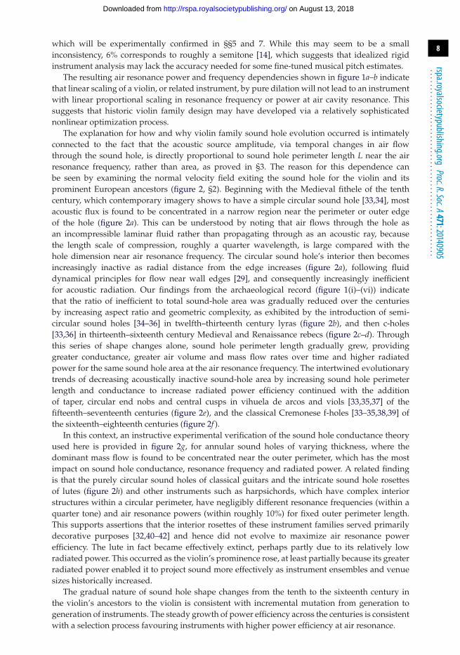
The explanation for how and why violin family sound hole evolution occurred is intimatelyconnected to the fact that the acoustic source amplitude, via temporal changes in air flowthrough the sound hole, is directly proportional to sound hole perimeter length L near the airresonance frequency, rather than area, as proved in §3. The reason for this dependence canbe seen by examining the normal velocity field exiting the sound hole for the violin and itsprominent European ancestors (figure 2, §2). Beginning with the Medieval fithele of the tenthcentury, which contemporary imagery shows to have a simple circular sound hole [33,34], mostacoustic flux is found to be concentrated in a narrow region near the perimeter or outer edgeof the hole (figure 2a). This can be understood by noting that air flows through the hole asan incompressible laminar fluid rather than propagating through as an acoustic ray, becausethe length scale of compression, roughly a quarter wavelength, is large compared with thehole dimension near air resonance frequency. The circular sound hole’s interior then becomesincreasingly inactive as radial distance from the edge increases (figure 2a), following fluiddynamical principles for flow near wall edges [29], and consequently increasingly inefficientfor acoustic radiation. Our findings from the archaeological record (figure 1(i)–(vi)) indicatethat the ratio of inefficient to total sound-hole area was gradually reduced over the centuriesby increasing aspect ratio and geometric complexity, as exhibited by the introduction of semi-circular sound holes [34–36] in twelfth–thirteenth century lyras (figure 2b), and then c-holes[33,36] in thirteenth–sixteenth century Medieval and Renaissance rebecs (figure 2c–d). Throughthis series of shape changes alone, sound hole perimeter length gradually grew, providinggreater conductance, greater air volume and mass flow rates over time and higher radiatedpower for the same sound hole area at the air resonance frequency. The intertwined evolutionarytrends of decreasing acoustically inactive sound-hole area by increasing sound hole perimeterlength and conductance to increase radiated power efficiency continued with the additionof taper, circular end nobs and central cusps in vihuela de arcos and viols [33,35,37] of thefifteenth–seventeenth centuries (figure 2e), and the classical Cremonese f-holes [33–35,38,39] ofthe sixteenth–eighteenth centuries (figure 2f ).
In this context, an instructive experimental verification of the sound hole conductance theoryused here is provided in figure 2g, for annular sound holes of varying thickness, where thedominant mass flow is found to be concentrated near the outer perimeter, which has the mostimpact on sound hole conductance, resonance frequency and radiated power. A related findingis that the purely circular sound holes of classical guitars and the intricate sound hole rosettesof lutes (figure 2h) and other instruments such as harpsichords, which have complex interiorstructures within a circular perimeter, have negligibly different resonance frequencies (within aquarter tone) and air resonance powers (within roughly 10%) for fixed outer perimeter length.This supports assertions that the interior rosettes of these instrument families served primarilydecorative purposes [32,40–42] and hence did not evolve to maximize air resonance powerefficiency. The lute in fact became effectively extinct, perhaps partly due to its relatively lowradiated power. This occurred as the violin’s prominence rose, at least partially because its greaterradiated power enabled it to project sound more effectively as instrument ensembles and venuesizes historically increased.
The gradual nature of sound hole shape changes from the tenth to the sixteenth century inthe violin’s ancestors to the violin is consistent with incremental mutation from generation togeneration of instruments. The steady growth of power efficiency across the centuries is consistentwith a selection process favouring instruments with higher power efficiency at air resonance.
on August 13, 2018http://rspa.royalsocietypublishing.org/Downloaded from
9
rspa.royalsocietypublishing.orgProc.R.Soc.A471:20140905
...................................................
(a) (b) (c)
(d)
(g) (h)
(e) ( f )
1.0
norm
aliz
ed f
requ
ency
f/f 0
cond
ucta
nce
C/C
0ra
diat
ed p
ower
P/P
0 0.9 f experimentf simulationC simulationP simulation0.8
0.7
0.6
0.5
0 0.2 0.4
d
D
0.6diameter ratio d/D
0.8 1.0
20/12
2–2/12
2–4/12
2–6/12
2–8/12
2–10/12
2–12/12
15
2.0
1.6
norm
aliz
ed f
low
vel
ocity
1.2
0.8
0.4
0
Figure 2. Sound hole shape evolution driven by maximization of efficient flow near outer perimeter, minimization of inactivesound-hole area and consequent maximization of acoustic conductance. Normal air velocity field un(x, y, z) (equation (2.2))through (a)–(f ) sound holes (i)–(vi) of figure 1 and (h) a lute rosette known as the ‘Warwick Frei’ [32] estimated for an infiniterigid soundhole bearingwall at air-resonance frequencies by boundary elementmethod in §2. (g) Experimental verification andillustration of the sound hole conductance theory for annular sound holes. Dashed horizontal lines indicate equal temperamentsemitone factors. The resonance frequency, conductance and radiated power of a circular sound hole are represented by f0, C0and P0, respectively. Velocities in (a)–(f ) and (h) are normalized by the average air-flow velocity through the circular soundhole (a).
on August 13, 2018http://rspa.royalsocietypublishing.org/Downloaded from
10
rspa.royalsocietypublishing.orgProc.R.Soc.A471:20140905
...................................................
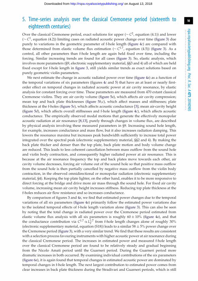
5. Time-series analysis over the classical Cremonese period (sixteenth toeighteenth centuries)
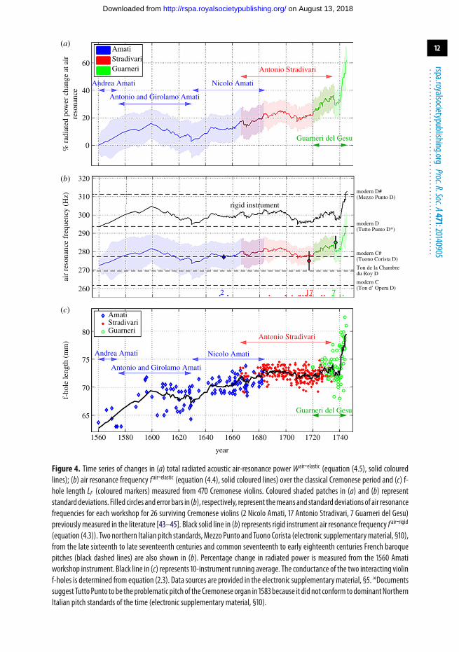
Over the classical Cremonese period, exact solutions for upper (∼ C2, equation (4.1)) and lower(∼ C1, equation (4.2)) limiting cases on radiated acoustic power change over time (figure 3) duepurely to variations in the geometric parameter of f-hole length (figure 4c) are compared withthose determined from elastic volume flux estimation (∼ C1.7, equation (4.5)) (figure 3). As acontrol, all other parameters than f-hole length are again held fixed over time, including theforcing. Similar increasing trends are found for all cases (figure 3). So, elastic analysis, whichinvolves more parameters (§9, electronic supplementary material, §§3 and 4) all of which are heldfixed except for f-hole length in figure 3, still yields similar trends as exact solutions based onpurely geometric violin parameters.
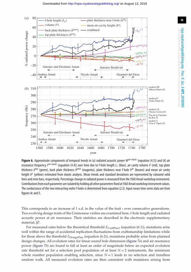
We next estimate the change in acoustic radiated power over time (figure 4a) as a function ofthe temporal variations of six parameters (figures 4c and 5) that have an at least or nearly first-order effect on temporal changes in radiated acoustic power at air cavity resonance, by elasticanalysis for constant forcing over time. These parameters are measured from 470 extant classicalCremonese violins. They are air cavity volume (figure 5a), which affects air cavity compression;mean top and back plate thicknesses (figure 5b,c), which affect masses and stiffnesses; platethickness at the f-holes (figure 5e), which affects acoustic conductance [3]; mean air-cavity height(figure 5d), which affects overall stiffnesses and f-hole length (figure 4c), which affects acousticconductance. The empirically observed modal motions that generate the effectively monopolaracoustic radiation at air resonance [8,13], purely through changes in volume flux, are describedby physical analysis involving these measured parameters in §9. Increasing sound hole length,for example, increases conductance and mass flow, but it also increases radiation damping. Thislowers the resonance maxima but increases peak bandwidth sufficiently to increase total powerintegrated over the spectral peak (electronic supplementary material, §§2 and 4). By making theback plate thicker and denser than the top plate, back plate motion and body volume changeare reduced. This leads to less coherent cancellation between mass outflow from the sound holeand violin body contraction, and consequently higher radiated power at air resonance. This isbecause at the air resonance frequency the top and back plates move towards each other, aircavity volume decreases, forcing air volume out of the sound hole so that positive mass outflowfrom the sound hole is then partially cancelled by negative mass outflow from the violin bodycontraction, in the observed omnidirectional or monopolar radiation (electronic supplementarymaterial, §4). Keeping the top plate lighter, on the other hand, enables it to be more responsive todirect forcing at the bridge and drive more air mass through the sound hole. For fixed air cavityvolume, increasing mean air cavity height increases stiffness. Reducing top plate thickness at thef-holes reduces air flow resistance and so increases conductance.
By comparison of figures 3 and 4a, we find that estimated power changes due to the temporalvariations of all six parameters (figure 4a) primarily follow the estimated power variations dueto the isolated temporal effects of f-hole length variation alone (figure 3). This can also be seenby noting that the total change in radiated power over the Cremonese period estimated fromelastic volume flux analysis with all six parameters is roughly 60 ± 10% (figure 4a), and thatthe conductance contribution via C1.7 ∝ L1.7
F from f-hole length changes alone of roughly 30%(electronic supplementary material, equation (S18)) leads to a similar 58 ± 5% power change overthe Cremonese period (figure 3), with a very similar trend. We find that these results are consistentwith a selection process favouring instruments with higher acoustic power at air resonance duringthe classical Cremonese period. The increases in estimated power and measured f-hole lengthover the classical Cremonese period are found to be relatively steady and gradual beginningfrom the Nicolo Amati period until the Guarneri period. During the Guarneri period moredramatic increases in both occurred. By examining individual contributions of the six parameters(figure 6a), it is again found that temporal changes in estimated acoustic power are dominated bytemporal changes in f-hole length. The next largest contribution to estimated power comes fromclear increases in back plate thickness during the Stradivari and Guarneri periods, which is still
on August 13, 2018http://rspa.royalsocietypublishing.org/Downloaded from

11
rspa.royalsocietypublishing.orgProc.R.Soc.A471:20140905
...................................................
80
60
40
20
0
1560 1580 1600 1620
infinite wall
C2
C1.7
C1
AmatiStradivari
Guarneri
rigid instrumentelastic instrument
1640 1660
year
variation in f-hole length only
% r
adia
ted
pow
er c
hang
e at
air
reso
nanc
e
1680 1700 1720 1740 1760
Figure 3. Time series of change in total radiated acoustic power as a function of temporal changes of the purely geometricparameter of f-hole length during the Cremonese period. The estimated dependence via elastic volume flux analysis(Wair-elastic ∼ C1.7, equation (4.5), solid coloured lines) is roughly the average of the upper (Wwall ∼ C2, equation (4.1), dashedblack line) and lower (Wair-rigid ∼ C, equation (4.2), solid black line) limiting cases. Coloured lines and shaded patches,respectively, represent mean trends and standard deviations of Wair-elastic for different workshops: Amati (blue), Stradivari(red), Guarneri (green), Amati–Stradivari overlap (blue-red) and Stradivari–Guarneri overlap (red-green). Percentage changeis measured from the 1560 Amati workshop instrument. The conductance of the two interacting violin f-holes is determinedfrom equation (2.3).
roughly a factor of two less than the contribution from f-hole length increases (figure 6a). Theseobservations and trends have clear design implications.
Mean air resonance frequencies estimated from elastic analysis match well, to within aneighth of a semitone corresponding to a roughly 1% RMSE, with mean measured air resonancefrequencies of classical Cremonese violins for each family workshop (figure 4b). Rigid instrumentanalysis leads to an air resonance frequency temporal trend similar to elastic analysis (figure 4b),suggesting that the elastic resonance frequency trend is dominated by variations in sound holelength and instrument volume. This is consistent with the finding that the effects of all otherparameters are small on the overall resonance frequency temporal trend (figure 6b), even thoughthey play an important role in fine tuning the absolute resonance frequency. Rigid instrumentanalysis, however, results in offsets of roughly a semitone between estimated and measuredCremonese air resonance frequencies (figure 4b), and so may not be sufficient for some fine-tuned musical applications. These observations and trends also have clear design implications.Increases in f-hole length (figure 4c) were apparently tempered by a gradual increasing trend incavity volume (figure 5a) that effectively constrained the air resonance frequency (equation (4.4))to vary within a semitone of traditional pitch conventions (figures 4b and 6b), and within a rangenot exceeding the resonance peak’s half power bandwidth, roughly its resolvable range.
6. Sound hole shape and air resonance power evolution rates and mechanismsA theoretical approach for determining whether design development is consistent with evolutionvia accidental replication fluctuations from craftsmanship limitations and subsequent selectionis developed and applied. Concepts and equations similar to those developed in biology forthe generational change in gene frequency solely due to random replication noise and naturalselection [46,47] are used. The formulation, however, includes thresholds for detecting changesin an evolving trait that are inconsistent with those expected solely from replication noise due torandom craftsmanship fluctuations, and so differs from biological formulations.
A key assumption is that the instrument makers select instruments for replication from acurrent pool within their workshop, which would typically be less or much less than the numberof surviving instruments in use at the time. This is consistent with historic evidence [38,39,48] andthe smooth nature of the time series in figure 4c.
on August 13, 2018http://rspa.royalsocietypublishing.org/Downloaded from
12
rspa.royalsocietypublishing.orgProc.R.Soc.A471:20140905
...................................................
60
40
20
0
320
310
300
290
280
air
reso
nanc
e fr
eque
ncy
(Hz)
270
260
% r
adia
ted
pow
er c
hang
e at
air
reso
nanc
e
AmatiStradivariGuarneri
rigid instrument
modern D#(Mezzo Punto D)
modern D(Tutto Punto D*)
modern C#(Tuono Corista D)
modern C(Ton d’ Opera D)
Ton de la Chambredu Roy D
Guarneri
80
75
70
f-ho
le le
ngth
(m
m)
65
1560 1580 1600 1620 1640
year
1660 1680 1700 1720 1740
AmatiStradivari
Antonio and Girolamo Amati
Andrea Amati Nicolo Amati
Antonio Stradivari
Guarneri del Gesu
7172
Antonio and Girolamo Amati
Andrea Amati Nicolo Amati
Antonio Stradivari
Guarneri del Gesu
(a)
(b)
(c)
Figure 4. Time series of changes in (a) total radiated acoustic air-resonance power Wair-elastic (equation (4.5), solid colouredlines); (b) air resonance frequency f air-elastic (equation (4.4), solid coloured lines) over the classical Cremonese period and (c) f-hole length LF (coloured markers) measured from 470 Cremonese violins. Coloured shaded patches in (a) and (b) representstandarddeviations. Filled circles anderror bars in (b), respectively, represent themeans and standarddeviations of air resonancefrequencies for each workshop for 26 surviving Cremonese violins (2 Nicolo Amati, 17 Antonio Stradivari, 7 Guarneri del Gesu)previouslymeasured in the literature [43–45]. Black solid line in (b) represents rigid instrument air resonance frequency f air-rigid
(equation (4.3)). Two northern Italian pitch standards,Mezzo Punto and Tuono Corista (electronic supplementarymaterial, §10),from the late sixteenth to late seventeenth centuries and common seventeenth to early eighteenth centuries French baroquepitches (black dashed lines) are also shown in (b). Percentage change in radiated power is measured from the 1560 Amatiworkshop instrument. Black line in (c) represents 10-instrument running average. The conductance of the two interacting violinf-holes is determined from equation (2.3). Data sources are provided in the electronic supplementary material, §5. *Documentssuggest Tutto Punto tobe theproblematic pitch of the Cremonese organ in 1583because it did not conform todominantNorthernItalian pitch standards of the time (electronic supplementary material, §10).
on August 13, 2018http://rspa.royalsocietypublishing.org/Downloaded from

13
rspa.royalsocietypublishing.orgProc.R.Soc.A471:20140905
...................................................
2000
1900
air
cavi
ty v
olum
e (c
m3 )
aver
age
thic
knes
s (m
m)
aver
age
thic
knes
s (m
m)
1800
1700
1600
4.0
3.5
3.0
2.5
2.0
4.0top plate
1560 1580 1600 1620 1640 1660
year
1680 1700 1720 1740
1560 1580 1600 1620 1640 1660
year
1680 1700 1720 1740
3.5
3.0
2.5
2.0
avra
ge th
ickn
ess
(mm
) 4.0
42back plate
near f-holes
40
38
36
mea
n ai
r-ca
vity
hei
ght (
mm
)
34
3.5
3.0
2.5
2.0
Antonio and Girolamo Amati
Antonio and Girolamo Amati
Antonio and Girolamo Amati
Antonio and Girolamo Amati
Antonio and Girolamo Amati
Andrea Amati
Andrea Amati
Andrea Amati
Andrea Amati
Andrea Amati
Nicolo Amati
Nicolo Amati
Nicolo Amati
Nicolo Amati
Nicolo Amati
Guarneri del GesuGuarneri del Gesu
Guarneri del GesuGuarneri del Gesu
Guarneri del Gesu
Antonio Stradivari
Antonio Stradivari
Antonio Stradivari
Antonio Stradivari
Antonio Stradivari
(a)
(b)
(d)
(e)
(c)
Figure 5. Temporal variations in (a) air-cavity volume V, (b) back plate thickness hback, (c) top plate thickness htop (d) platethickness near f-holes hsh and (e) mean air cavity height ha measured from 110 classical Cremonese violins. Black lines in (a,e)represent 20-instrument running averages, and in (b)–(d) represent quadratic regression fits of available thickness data. Datasources are provided in the electronic supplementary material, §5.
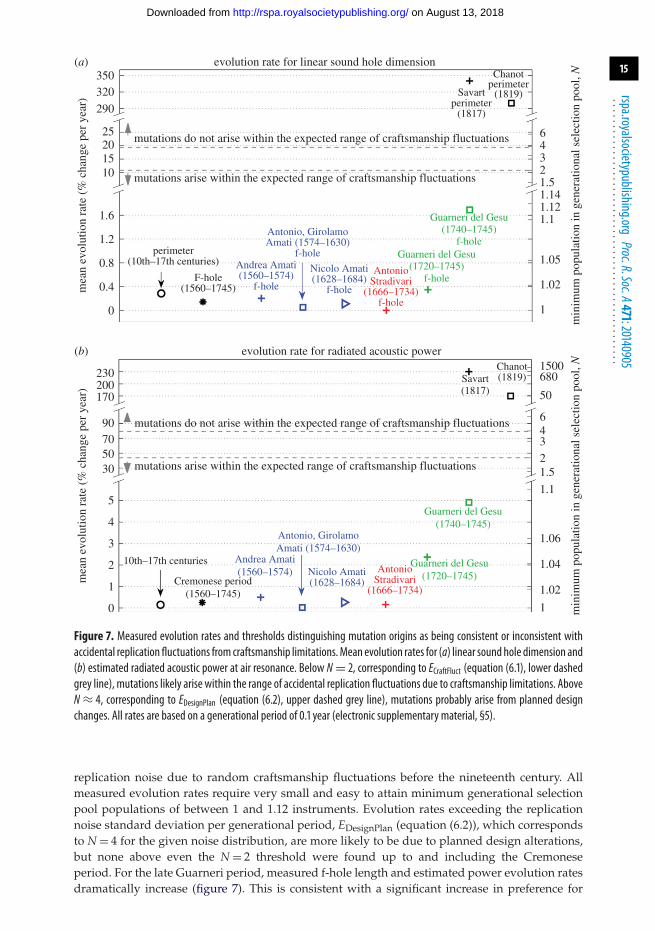
The expected evolution rate threshold ECraftFluct is defined as the difference from the meanof the expected maximum value of the evolving random trait variable, taken from the expectedselection pool of population N containing the most recent generations, divided by the mean timebetween each generation, assuming randomness and mutation solely due to random replicationnoise. So, the evolution rate threshold, ECraftFluct, for a given trait ι, such as f-hole length,below which trait evolution rates are consistent with accidental trait replication fluctuations fromcraftsmanship limitations is defined as
ECraftFluct = 〈maxN(ι)〉 − 〈ι〉Tg
. (6.1)
Here maxN(ι) represents the maximum value of the trait ι taken from a selection pool ofpopulation N containing the most recent generations, 〈ι〉 is the expected value of ι and Tg isthe mean generational period. Equation (6.1) reduces to that for expected generational changein gene frequency due to replication error and natural selection obtained by Price [46] whenonly the sample with the largest trait value is selected for replication. Another evolutionrate threshold, EDesignPlan, above which trait evolution rates are likely to be inconsistent withaccidental replication fluctuations from craftsmanship limitations is defined as
EDesignPlan =√
〈ι2〉 − 〈ι〉2
Tg. (6.2)
on August 13, 2018http://rspa.royalsocietypublishing.org/Downloaded from
14
rspa.royalsocietypublishing.orgProc.R.Soc.A471:20140905
...................................................
80f-hole length (LF) plate thickness near f-hole (hsh)
mean air-cavity height (ha)
combined
volume (V)
back plate thickness (hback)
top plate thickness (htop)
Antonio and Girolamo Amati
Antonio and Girolamo Amati
Andrea Amati
Andrea Amati
Nicolo Amati
Nicolo Amati
Antonio Stradivari
Antonio Stradivari
Guarneri del Gesu
Guarneri del Gesu
60
40
20
0
–20
–40
310
300
290
280
270
260
freq
uenc
y (H
z)%
rad
iate
d po
wer
cha
nge
250
240
2301560 1580 1600 1620 1640 1660 1680 1700
year1720 1740 1760
~LF1.7
~(hback)0.6
~(htop)–0.2
~(hsh)–0.5
~(ha)–0.9
~V–0.8
~LF0.5
~(hback)0.1
~(ha)0.2
~V–0.6
~(hsh)–0.1
~(htop)0.01
modern D#(Mezzo Punto D)
modern D(Tutto Punto D)
modern C#(Tuono Corista D)
modern C(Ton d’ Opera D)
Ton de la Chambredu Roy D
(a)
(b)
Figure 6. Approximate components of temporal trends in (a) radiated acoustic power Wair-elastic (equation (4.5)) and (b) airresonance frequency f air-elastic (equation (4.4)) over time due to f-hole length LF (blue), air cavity volume V (red), top platethickness htop (green), back plate thickness hback (magenta), plate thickness near f-hole hsh (brown) and mean air cavityheight ha (yellow) estimated from elastic analysis. Mean trends and standard deviations are represented by coloured solidlines and error bars, respectively. Percentage change in radiated power is measured from the 1560 Amati workshop instrument.Contributions fromeachparameter are isolatedbyholding all other parameters fixed at 1560Amatiworkshop instrument values.The conductance of the two interacting violin f-holes is determined from equation (2.3). Input mean time series data are fromfigures 4c and 5.
This corresponds to an increase of 1 s.d. in the value of the trait ι over consecutive generations.Two evolving design traits of the Cremonese violins are examined here, f-hole length and radiatedacoustic power at air resonance. Their statistics are described in the electronic supplementarymaterial, §7.
For measured rates below the theoretical threshold ECraftFluct (equation (6.1)), mutations arisewell within the range of accidental replication fluctuations from craftsmanship limitations whilefor those above the threshold EDesignPlan (equation (6.2)), mutations probably arise from planneddesign changes. All evolution rates for linear sound hole dimension (figure 7a) and air resonancepower (figure 7b) are found to fall at least an order of magnitude below an expected evolutionrate threshold set for a selection pool population of at least N = 2 instruments, the minimumwhole number population enabling selection, since N = 1 leads to no selection and trendlessrandom walk. All measured evolution rates are then consistent with mutations arising from
on August 13, 2018http://rspa.royalsocietypublishing.org/Downloaded from
15
rspa.royalsocietypublishing.orgProc.R.Soc.A471:20140905
...................................................
evolution rate for linear sound hole dimension350320
290
25201510
1.6
mutations arise within the expected range of craftsmanship fluctuations
mutations do not arise within the expected range of craftsmanship fluctuations
evolution rate for radiated acoustic power
mutations arise within the expected range of craftsmanship fluctuations
mutations do not arise within the expected range of craftsmanship fluctuations
1.2
mea
n ev
olut
ion
rate
(%
cha
nge
per
year
)
min
imum
pop
ulat
ion
in g
ener
atio
nal s
elec
tion
pool
, Nm
inim
um p
opul
atio
n in
gen
erat
iona
l sel
ectio
n po
ol, N
perimeter(10th–17th centuries)
F-hole(1560–1745)
Andrea Amati(1560–1574)
f-hole
Andrea Amati(1560–1574)
Antonio, GirolamoAmati (1574–1630)
f-hole
Guarneri del Gesu(1740–1745)
f-holeGuarneri del Gesu
(1720–1745)f-hole
Nicolo Amati(1628–1684)
f-hole
AntonioStradivari
(1666–1734)f-hole
0.8
0.4
0
230200170
90705030
5
4
3
mea
n ev
olut
ion
rate
(%
cha
nge
per
year
)
2
1
0
Savartperimeter
(1817)
Chanotperimeter
(1819)
64321.51.141.121.1
1.05
1.02
1
Savart(1817)
Chanot(1819)
1500680
50
64321.5
1.1
1.06
1.04
1.02
1
Antonio, GirolamoAmati (1574–1630)
Nicolo Amati(1628–1684)
AntonioStradivari
(1666–1734)
Guarneri del Gesu(1740–1745)
Guarneri del Gesu(1720–1745)
10th–17th centuries
Cremonese period(1560–1745)
(a)
(b)
Figure 7. Measured evolution rates and thresholds distinguishing mutation origins as being consistent or inconsistent withaccidental replication fluctuations from craftsmanship limitations.Mean evolution rates for (a) linear sound hole dimension and(b) estimated radiated acoustic power at air resonance. Below N = 2, corresponding to ECraftFluct (equation (6.1), lower dashedgrey line), mutations likely arise within the range of accidental replication fluctuations due to craftsmanship limitations. AboveN ≈ 4, corresponding to EDesignPlan (equation (6.2), upper dashed grey line), mutations probably arise from planned designchanges. All rates are based on a generational period of 0.1 year (electronic supplementary material, §5).
replication noise due to random craftsmanship fluctuations before the nineteenth century. Allmeasured evolution rates require very small and easy to attain minimum generational selectionpool populations of between 1 and 1.12 instruments. Evolution rates exceeding the replicationnoise standard deviation per generational period, EDesignPlan (equation (6.2)), which correspondsto N = 4 for the given noise distribution, are more likely to be due to planned design alterations,but none above even the N = 2 threshold were found up to and including the Cremoneseperiod. For the late Guarneri period, measured f-hole length and estimated power evolution ratesdramatically increase (figure 7). This is consistent with a significant increase in preference for
on August 13, 2018http://rspa.royalsocietypublishing.org/Downloaded from
16
rspa.royalsocietypublishing.orgProc.R.Soc.A471:20140905
...................................................
Savart Chanot
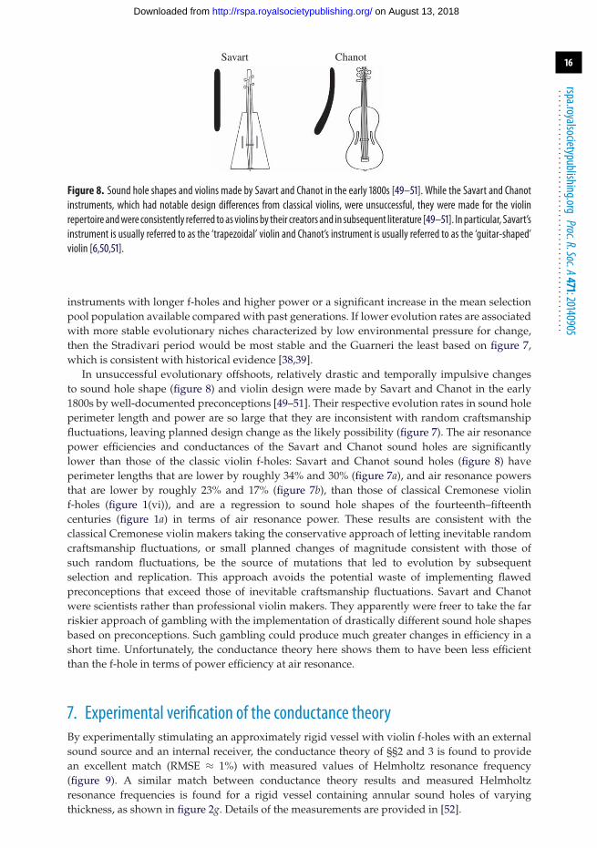
Figure 8. Sound hole shapes and violins made by Savart and Chanot in the early 1800s [49–51]. While the Savart and Chanotinstruments, which had notable design differences from classical violins, were unsuccessful, they were made for the violinrepertoire andwere consistently referred to as violins by their creators and in subsequent literature [49–51]. In particular, Savart’sinstrument is usually referred to as the ‘trapezoidal’ violin and Chanot’s instrument is usually referred to as the ‘guitar-shaped’violin [6,50,51].
instruments with longer f-holes and higher power or a significant increase in the mean selectionpool population available compared with past generations. If lower evolution rates are associatedwith more stable evolutionary niches characterized by low environmental pressure for change,then the Stradivari period would be most stable and the Guarneri the least based on figure 7,which is consistent with historical evidence [38,39].
In unsuccessful evolutionary offshoots, relatively drastic and temporally impulsive changesto sound hole shape (figure 8) and violin design were made by Savart and Chanot in the early1800s by well-documented preconceptions [49–51]. Their respective evolution rates in sound holeperimeter length and power are so large that they are inconsistent with random craftsmanshipfluctuations, leaving planned design change as the likely possibility (figure 7). The air resonancepower efficiencies and conductances of the Savart and Chanot sound holes are significantlylower than those of the classic violin f-holes: Savart and Chanot sound holes (figure 8) haveperimeter lengths that are lower by roughly 34% and 30% (figure 7a), and air resonance powersthat are lower by roughly 23% and 17% (figure 7b), than those of classical Cremonese violinf-holes (figure 1(vi)), and are a regression to sound hole shapes of the fourteenth–fifteenthcenturies (figure 1a) in terms of air resonance power. These results are consistent with theclassical Cremonese violin makers taking the conservative approach of letting inevitable randomcraftsmanship fluctuations, or small planned changes of magnitude consistent with those ofsuch random fluctuations, be the source of mutations that led to evolution by subsequentselection and replication. This approach avoids the potential waste of implementing flawedpreconceptions that exceed those of inevitable craftsmanship fluctuations. Savart and Chanotwere scientists rather than professional violin makers. They apparently were freer to take the farriskier approach of gambling with the implementation of drastically different sound hole shapesbased on preconceptions. Such gambling could produce much greater changes in efficiency in ashort time. Unfortunately, the conductance theory here shows them to have been less efficientthan the f-hole in terms of power efficiency at air resonance.
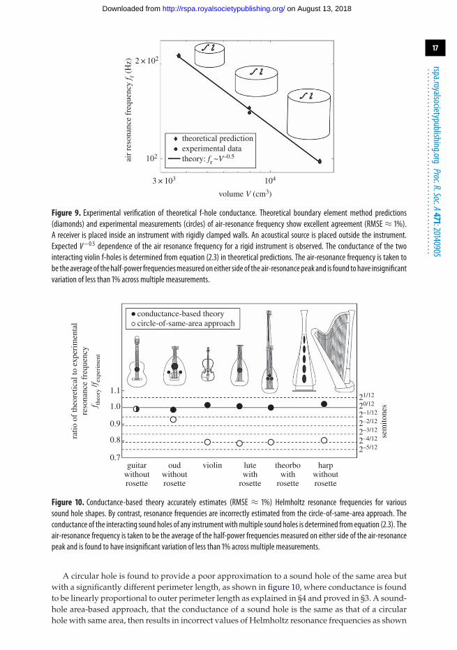
7. Experimental verification of the conductance theoryBy experimentally stimulating an approximately rigid vessel with violin f-holes with an externalsound source and an internal receiver, the conductance theory of §§2 and 3 is found to providean excellent match (RMSE ≈ 1%) with measured values of Helmholtz resonance frequency(figure 9). A similar match between conductance theory results and measured Helmholtzresonance frequencies is found for a rigid vessel containing annular sound holes of varyingthickness, as shown in figure 2g. Details of the measurements are provided in [52].
on August 13, 2018http://rspa.royalsocietypublishing.org/Downloaded from
17
rspa.royalsocietypublishing.orgProc.R.Soc.A471:20140905
...................................................
104
102
theoretical predictionexperimental datatheory: fr ~V–0.5
3 × 10³
2 × 10²
volume V (cm3)
air
reso
nanc
e fr
eque
ncy
f r (H
z)
Figure 9. Experimental verification of theoretical f-hole conductance. Theoretical boundary element method predictions(diamonds) and experimental measurements (circles) of air-resonance frequency show excellent agreement (RMSE ≈ 1%).A receiver is placed inside an instrument with rigidly clamped walls. An acoustical source is placed outside the instrument.Expected V−0.5 dependence of the air resonance frequency for a rigid instrument is observed. The conductance of the twointeracting violin f-holes is determined from equation (2.3) in theoretical predictions. The air-resonance frequency is taken tobe theaverageof thehalf-power frequenciesmeasuredoneither sideof the air-resonancepeakand is found tohave insignificantvariation of less than 1% across multiple measurements.
1.1
conductance-based theorycircle-of-same-area approach
ratio
of
theo
retic
al to
exp
erim
enta
lre
sona
nce
freq
uenc
yf th
eory
/fex
peri
men
t
1.0
0.9
0.8
0.7guitar
withoutrosette
oudwithoutrosette
lutewith
rosette
theorbowith
rosette
harpwithoutrosette
sem
itone
s
21/12
20/12
2–1/12
2–2/12
2–3/12
2–4/12
2–5/12
violin
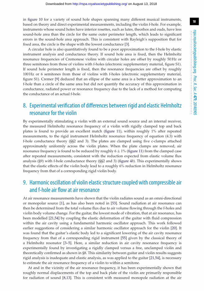
Figure 10. Conductance-based theory accurately estimates (RMSE ≈ 1%) Helmholtz resonance frequencies for varioussound hole shapes. By contrast, resonance frequencies are incorrectly estimated from the circle-of-same-area approach. Theconductance of the interacting sound holes of any instrument withmultiple sound holes is determined from equation (2.3). Theair-resonance frequency is taken to be the average of the half-power frequencies measured on either side of the air-resonancepeak and is found to have insignificant variation of less than 1% across multiple measurements.
A circular hole is found to provide a poor approximation to a sound hole of the same area butwith a significantly different perimeter length, as shown in figure 10, where conductance is foundto be linearly proportional to outer perimeter length as explained in §4 and proved in §3. A sound-hole area-based approach, that the conductance of a sound hole is the same as that of a circularhole with same area, then results in incorrect values of Helmholtz resonance frequencies as shown
on August 13, 2018http://rspa.royalsocietypublishing.org/Downloaded from
18
rspa.royalsocietypublishing.orgProc.R.Soc.A471:20140905
...................................................
in figure 10 for a variety of sound hole shapes spanning many different musical instruments,based on theory and direct experimental measurements, including the violin f-hole. For example,instruments whose sound holes have interior rosettes, such as lutes, theorbos and ouds, have lesssound-hole area than the circle for the same outer perimeter length, which leads to significanterrors in the sound-hole area approach. This is consistent with Rayleigh’s supposition that forfixed area, the circle is the shape with the lowest conductance [3].
A circular hole is also quantitatively found to be a poor approximation to the f-hole by elasticinstrument analysis and conductance theory. If sound hole area is fixed, then the Helmholtzresonance frequencies of Cremonese violins with circular holes are offset by roughly 50 Hz orthree semitones from those of violins with f-holes (electronic supplementary material, figure S1).If sound hole perimeter length is fixed, then the resonance frequencies are offset by roughly100 Hz or 6 semitones from those of violins with f-holes (electronic supplementary material,figure S1). Cremer [9] deduced that an ellipse of the same area is a better approximation to anf-hole than a circle of the same area but did not quantify the accuracy of this approximation inconductance, radiated power or resonance frequency due to the lack of a method for computingthe conductance of an actual f-hole.
8. Experimental verification of differences between rigid and elastic Helmholtzresonance for the violin
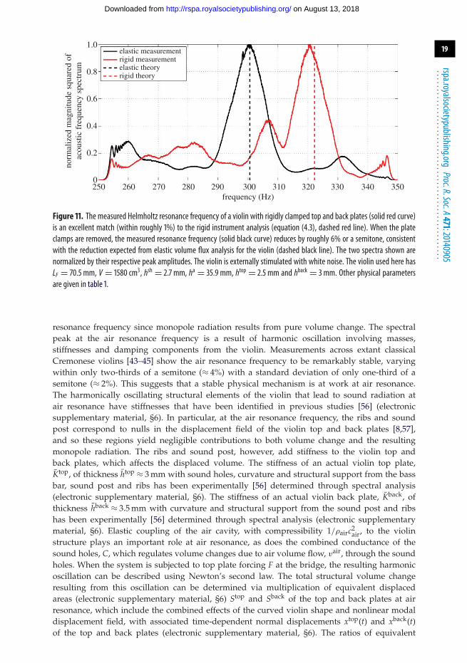
By experimentally stimulating a violin with an external sound source and an internal receiver,the measured Helmholtz resonance frequency of a violin with rigidly clamped top and backplates is found to provide an excellent match (figure 11), within roughly 1% after repeatedmeasurements, to the rigid instrument Helmholtz resonance frequency of equation (4.3) withf-hole conductance theory (§§2 and 3). The plates are clamped using five c-clamps attachedapproximately uniformly across the violin plates. When the plate clamps are removed, airresonance frequency is found to be reduced by roughly 6 ± 1% (figure 11) from the clamped caseafter repeated measurements, consistent with the reduction expected from elastic volume fluxanalysis (§9) with f-hole conductance theory (§§2 and 3) (figure 4b). This experimentally showsthat the elastic effects of the violin body lead to a roughly 6% reduction in Helmholtz resonancefrequency from that of a corresponding rigid violin body.
9. Harmonic oscillation of violin elastic structure coupled with compressible airand f-hole air flow at air resonance
At air resonance measurements have shown that the violin radiates sound as an omni-directionalor monopolar source [1], as has also been noted in [53]. Sound radiation at air resonance canthen be determined from the total volume flux due to air volume flowing through the f-holes andviolin body volume change. For the guitar, the lowest mode of vibration, that at air resonance, hasbeen modelled [21,54] by coupling the elastic deformation of the guitar with fluid compressionwithin the air cavity using a fundamental harmonic oscillator approach. This work followedearlier suggestions of considering a similar harmonic oscillator approach for the violin [20]. Itwas found that the guitar’s elastic body led to a significant lowering of the air cavity resonancefrequency from that of a corresponding rigid instrument [55] given by the classical theory ofa Helmholtz resonator [3–5]. Here, a similar reduction in air cavity resonance frequency isexperimentally found by investigating a rigidly clamped versus a free, unclamped violin andtheoretically confirmed as shown in §8. This similarity between guitar and violin results suggestsrigid analysis is inadequate and elastic analysis, as was applied to the guitar [21,54], is necessaryto estimate the air resonance frequency of a violin to within a semitone.
At and in the vicinity of the air resonance frequency, it has been experimentally shown thatroughly normal displacements of the top and back plate of the violin are primarily responsiblefor radiation of sound [8,13]. This is consistent with measured monopole radiation at the air
on August 13, 2018http://rspa.royalsocietypublishing.org/Downloaded from
19
rspa.royalsocietypublishing.orgProc.R.Soc.A471:20140905
...................................................
250 260 270
1.0
0.8
elastic measurementrigid measurementelastic theoryrigid theory
0.6
norm
aliz
ed m
agni
tude
squ
ared
of
acou
stic
fre
quen
cy s
pect
rum
0.4
0.2
0280 290 300 310
frequency (Hz)320 330 340 350
Figure 11. The measured Helmholtz resonance frequency of a violin with rigidly clamped top and back plates (solid red curve)is an excellent match (within roughly 1%) to the rigid instrument analysis (equation (4.3), dashed red line). When the plateclamps are removed, the measured resonance frequency (solid black curve) reduces by roughly 6% or a semitone, consistentwith the reduction expected from elastic volume flux analysis for the violin (dashed black line). The two spectra shown arenormalized by their respective peak amplitudes. The violin is externally stimulated with white noise. The violin used here hasLF = 70.5 mm, V = 1580 cm3, hsh = 2.7 mm, ha = 35.9 mm, htop = 2.5 mm and hback = 3 mm. Other physical parametersare given in table 1.
resonance frequency since monopole radiation results from pure volume change. The spectralpeak at the air resonance frequency is a result of harmonic oscillation involving masses,stiffnesses and damping components from the violin. Measurements across extant classicalCremonese violins [43–45] show the air resonance frequency to be remarkably stable, varyingwithin only two-thirds of a semitone (≈ 4%) with a standard deviation of only one-third of asemitone (≈ 2%). This suggests that a stable physical mechanism is at work at air resonance.The harmonically oscillating structural elements of the violin that lead to sound radiation atair resonance have stiffnesses that have been identified in previous studies [56] (electronicsupplementary material, §6). In particular, at the air resonance frequency, the ribs and soundpost correspond to nulls in the displacement field of the violin top and back plates [8,57],and so these regions yield negligible contributions to both volume change and the resultingmonopole radiation. The ribs and sound post, however, add stiffness to the violin top andback plates, which affects the displaced volume. The stiffness of an actual violin top plate,Ktop, of thickness htop ≈ 3 mm with sound holes, curvature and structural support from the bassbar, sound post and ribs has been experimentally [56] determined through spectral analysis(electronic supplementary material, §6). The stiffness of an actual violin back plate, Kback, ofthickness hback ≈ 3.5 mm with curvature and structural support from the sound post and ribshas been experimentally [56] determined through spectral analysis (electronic supplementarymaterial, §6). Elastic coupling of the air cavity, with compressibility 1/ρairc2
air, to the violinstructure plays an important role at air resonance, as does the combined conductance of thesound holes, C, which regulates volume changes due to air volume flow, vair, through the soundholes. When the system is subjected to top plate forcing F at the bridge, the resulting harmonicoscillation can be described using Newton’s second law. The total structural volume changeresulting from this oscillation can be determined via multiplication of equivalent displacedareas (electronic supplementary material, §6) Stop and Sback of the top and back plates at airresonance, which include the combined effects of the curved violin shape and nonlinear modaldisplacement field, with associated time-dependent normal displacements xtop(t) and xback(t)of the top and back plates (electronic supplementary material, §6). The ratios of equivalent
on August 13, 2018http://rspa.royalsocietypublishing.org/Downloaded from
20
rspa.royalsocietypublishing.orgProc.R.Soc.A471:20140905
...................................................
displaced area to total plate surface area for actual violin top and back plates at air resonancehave been experimentally determined (electronic supplementary material, §6) from holographicmeasurements [57].
The air-resonance dynamics of i = 1, 2, 3, . . . N Cremonese violins beginning from Amati1560 to Guarneri 1745, where N = 485 are analysed. Known design parameters Ci (electronicsupplementary material, §9), Vi, htop
i , hbacki and ha
i from direct measurements or interpolation
appear in figures 4c and 5. Small variations in top plate thickness htopi about htop for the ith violin
lead to top plate stiffness Ktopi = Ktop + εtop[htop
i − htop] near air resonance where εtop is the first-order Taylor series coefficient. Similarly, back plate stiffness Kback
i = Kback + εback[hbacki − hback]
near air resonance depends on plate thickness hbacki , where εback is the first-order Taylor series
coefficient for small variations near hback. The equivalent displaced top plate and back plateareas (electronic supplementary material, §6) that contribute to acoustic radiation via net volumechange near air resonance are given by Stop
i = ξ topAtopi and Sback
i = ξbackAbacki , where Atop
i = Vi/hai
and Abacki = Vi/ha
i are the total top and back plate areas. The displaced masses of the top and
back plates near air resonance are then Mtopi = ρtophtop
i Stopi and Mback
i = ρbackhbacki Sback
i . Dampingfactors at air resonance
Rairi ≈ ρair
4πcair(ωair
i )2, Rtopi ≈ ρair(Stop
i )2
4πcair(ωair
i )2,
Rbacki ≈ ρair(Sback
i )2
4πcair(ωair
i )2
and Rtop-backi ≈ ρair(Stop
i )2
4πcair(ωair
i )2, Rback-topi ≈ ρair(Sback
i )2
4πcair(ωair
i )2
⎫⎪⎪⎪⎪⎪⎪⎪⎪⎪⎪⎪⎪⎬⎪⎪⎪⎪⎪⎪⎪⎪⎪⎪⎪⎪⎭
(9.1)
are determined such that the energy dissipated by the damping forces acting on the plates andair piston is equal to that acoustically radiated from plate oscillations and air flow through thesound holes (electronic supplementary material, §3), where constants ρtop and ρback are top andback plate densities, respectively. Viscous air flow damping at the sound hole is at least oneorder of magnitude smaller than radiation damping [10] at air resonance and is negligible. In theguitar model [21,54], damping coefficients were empirically determined by matching modelledand measured sound spectra and/or plate mobility. The physical approach for determining thedamping coefficients used here follows Lamb [4], through a radiation damping mechanism. TheQ-factors obtained here for the air resonance peaks and the corresponding half power bandwidthare within roughly 20% of those measured for violins [13,58], indicating that radiation dampingis the dominant source of damping at the air resonance frequency.
Narrowband [31,59–61] forcing F(t) ≈ F0(t) e−jωairi t that is spectrally constant in the vicinity
of the air resonance peak ωairi is assumed, where F0(t) is a slowly varying temporal envelope
that is the same for each of the i = 1, 2, 3, . . . N violins. This allows narrowband approximations[31,59–61] for the displacements xtop
i (t) ≈ χtopi (t) e−jωair
i t , xbacki (t) ≈ χback
i (t) e−jωairi t and vair
i (t) ≈γ air
i (t) e−jωairi t, where χ
topi (t), χback
i (t) and γ airi (t) are slowly varying temporal envelopes that are
effectively constant at the center of the time window for the ith violin. The harmonic oscillatingsystem at air resonance for the ith violin can then be described by
⎛⎜⎜⎝
B11 B12 B13
B21 B22 B23
B31 B32 B33
⎞⎟⎟⎠
⎛⎜⎜⎜⎝
xtopi (t)
xbacki (t)
vairi (t)
⎞⎟⎟⎟⎠ =
⎛⎜⎝F(t)
00
⎞⎟⎠ , (9.2)
on August 13, 2018http://rspa.royalsocietypublishing.org/Downloaded from
21
rspa.royalsocietypublishing.orgProc.R.Soc.A471:20140905
...................................................
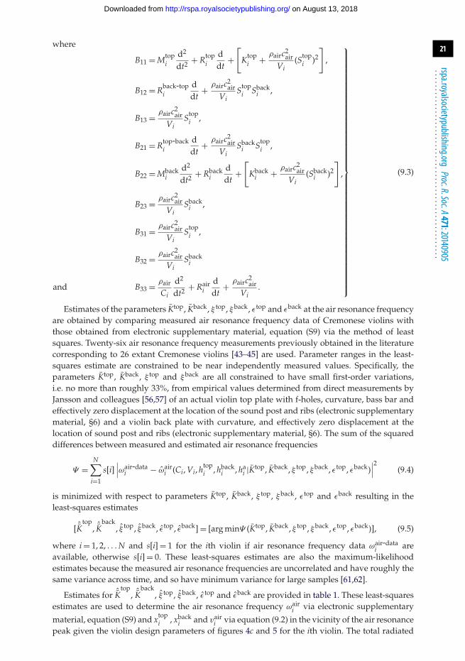
where
B11 = Mtopi
d2
dt2 + Rtopi
ddt
+[
Ktopi + ρairc2
airVi
(Stopi )2
],
B12 = Rback-topi
ddt
+ ρairc2air
ViStop
i Sbacki ,
B13 = ρairc2air
ViStop
i ,
B21 = Rtop-backi
ddt
+ ρairc2air
ViSback
i Stopi ,
B22 = Mbacki
d2
dt2 + Rbacki
ddt
+[
Kbacki + ρairc2
airVi
(Sbacki )2
],
B23 = ρairc2air
ViSback
i ,
B31 = ρairc2air
ViStop
i ,
B32 = ρairc2air
ViSback
i
and B33 = ρair
Ci
d2
dt2 + Rairi
ddt
+ ρairc2air
Vi.
⎫⎪⎪⎪⎪⎪⎪⎪⎪⎪⎪⎪⎪⎪⎪⎪⎪⎪⎪⎪⎪⎪⎪⎪⎪⎪⎪⎪⎪⎪⎪⎪⎪⎪⎪⎪⎪⎪⎪⎪⎪⎪⎪⎪⎬⎪⎪⎪⎪⎪⎪⎪⎪⎪⎪⎪⎪⎪⎪⎪⎪⎪⎪⎪⎪⎪⎪⎪⎪⎪⎪⎪⎪⎪⎪⎪⎪⎪⎪⎪⎪⎪⎪⎪⎪⎪⎪⎪⎭
(9.3)
Estimates of the parameters Ktop, Kback, ξ top, ξback, εtop and εback at the air resonance frequencyare obtained by comparing measured air resonance frequency data of Cremonese violins withthose obtained from electronic supplementary material, equation (S9) via the method of leastsquares. Twenty-six air resonance frequency measurements previously obtained in the literaturecorresponding to 26 extant Cremonese violins [43–45] are used. Parameter ranges in the least-squares estimate are constrained to be near independently measured values. Specifically, theparameters Ktop, Kback, ξ top and ξback are all constrained to have small first-order variations,i.e. no more than roughly 33%, from empirical values determined from direct measurements byJansson and colleagues [56,57] of an actual violin top plate with f-holes, curvature, bass bar andeffectively zero displacement at the location of the sound post and ribs (electronic supplementarymaterial, §6) and a violin back plate with curvature, and effectively zero displacement at thelocation of sound post and ribs (electronic supplementary material, §6). The sum of the squareddifferences between measured and estimated air resonance frequencies
Ψ =N∑
i=1
s[i]∣∣∣ωair-data
i − ωairi (Ci, Vi, htop
i , hbacki , ha
i |Ktop, Kback, ξ top, ξback, εtop, εback)∣∣∣2 (9.4)
is minimized with respect to parameters Ktop, Kback, ξ top, ξback, εtop and εback resulting in theleast-squares estimates
[ ˆKtop
, ˆKback
, ξ top, ξback, εtop, εback] = [arg minΨ (Ktop, Kback, ξ top, ξback, εtop, εback)], (9.5)
where i = 1, 2, . . . N and s[i] = 1 for the ith violin if air resonance frequency data ωair-datai are
available, otherwise s[i] = 0. These least-squares estimates are also the maximum-likelihoodestimates because the measured air resonance frequencies are uncorrelated and have roughly thesame variance across time, and so have minimum variance for large samples [61,62].
Estimates for ˆKtop
, ˆKback
, ξ top, ξback, εtop and εback are provided in table 1. These least-squaresestimates are used to determine the air resonance frequency ωair
i via electronic supplementary
material, equation (S9) and xtopi , xback
i and vairi via equation (9.2) in the vicinity of the air resonance
peak given the violin design parameters of figures 4c and 5 for the ith violin. The total radiated
on August 13, 2018http://rspa.royalsocietypublishing.org/Downloaded from

22
rspa.royalsocietypublishing.orgProc.R.Soc.A471:20140905
...................................................
Table 1. Parameters estimated in elastic volume flux analysis.
parameter value
ˆKtopfor htop = 3 mm 6.92 × 10⁴ N m−1
. . . . . . . . . . . . . . . . . . . . . . . . . . . . . . . . . . . . . . . . . . . . . . . . . . . . . . . . . . . . . . . . . . . . . . . . . . . . . . . . . . . . . . . . . . . . . . . . . . . . . . . . . . . . . . . . . . . . . . . . . . . . . . . . . . . . . . . . . . . . . . . . . . . . . . . . . . . . . . . . . . . . . . . . . . . . . . . . . . . . . . . . . . . . . . . . . . . . . . . . . .
ˆKback
for hback = 3.5 mm 2.75 × 10⁵ N m−1. . . . . . . . . . . . . . . . . . . . . . . . . . . . . . . . . . . . . . . . . . . . . . . . . . . . . . . . . . . . . . . . . . . . . . . . . . . . . . . . . . . . . . . . . . . . . . . . . . . . . . . . . . . . . . . . . . . . . . . . . . . . . . . . . . . . . . . . . . . . . . . . . . . . . . . . . . . . . . . . . . . . . . . . . . . . . . . . . . . . . . . . . . . . . . . . . . . . . . . . . .
ε top for top plate thickness variation near htop 1.10 × 10⁷ N m−2. . . . . . . . . . . . . . . . . . . . . . . . . . . . . . . . . . . . . . . . . . . . . . . . . . . . . . . . . . . . . . . . . . . . . . . . . . . . . . . . . . . . . . . . . . . . . . . . . . . . . . . . . . . . . . . . . . . . . . . . . . . . . . . . . . . . . . . . . . . . . . . . . . . . . . . . . . . . . . . . . . . . . . . . . . . . . . . . . . . . . . . . . . . . . . . . . . . . . . . . . .
εback for back plate thickness variation near hback 1.20 × 10⁸ N m−2. . . . . . . . . . . . . . . . . . . . . . . . . . . . . . . . . . . . . . . . . . . . . . . . . . . . . . . . . . . . . . . . . . . . . . . . . . . . . . . . . . . . . . . . . . . . . . . . . . . . . . . . . . . . . . . . . . . . . . . . . . . . . . . . . . . . . . . . . . . . . . . . . . . . . . . . . . . . . . . . . . . . . . . . . . . . . . . . . . . . . . . . . . . . . . . . . . . . . . . . . .
ξ top 0.15. . . . . . . . . . . . . . . . . . . . . . . . . . . . . . . . . . . . . . . . . . . . . . . . . . . . . . . . . . . . . . . . . . . . . . . . . . . . . . . . . . . . . . . . . . . . . . . . . . . . . . . . . . . . . . . . . . . . . . . . . . . . . . . . . . . . . . . . . . . . . . . . . . . . . . . . . . . . . . . . . . . . . . . . . . . . . . . . . . . . . . . . . . . . . . . . . . . . . . . . . .
ξ back 0.22. . . . . . . . . . . . . . . . . . . . . . . . . . . . . . . . . . . . . . . . . . . . . . . . . . . . . . . . . . . . . . . . . . . . . . . . . . . . . . . . . . . . . . . . . . . . . . . . . . . . . . . . . . . . . . . . . . . . . . . . . . . . . . . . . . . . . . . . . . . . . . . . . . . . . . . . . . . . . . . . . . . . . . . . . . . . . . . . . . . . . . . . . . . . . . . . . . . . . . . . . .
power at air-resonance is then determined from the resulting xtopi , xback
i and vairi via equation (9.8)
for the ith violin. This leads to the time series of air resonance frequency and power shown infigure 4a–b. Empirically obtained dependencies of the air resonance frequency and power onviolin design parameters over the entire Cremonese period are given in equations (4.4) and (4.5),respectively. Time series of estimated air-resonance frequency and half power bandwidth aboutthe resonant peak, determined from equation (9.7) (electronic supplementary material, figure S2),characterize the resonance peaks estimated for each violin in the time series [63]. Wood densitiesare taken to be ρtop = 400 kg m−3, ρback = 600 kg m−3 [8] and air densities and sound speeds aretaken to be cair = 340 m s−1 and ρair = 1 kg m−3 [64].
The second and third eigenvalues, where ωMode-1i < ωMode-2
i < ωMode-3i and ωMode-1
i = ωairi of
the equation (9.2) system are also estimated from electronic supplementary material, equationS9 for all i = 1, 2, 3 . . . N violins with the parameters of table 1. The RMSE between the meansof estimated first eigenvalues and those measured [43–45] from classical Cremonese violins foreach family workshop is roughly 1%. Over the entire Cremonese period, the second and thirdeigenvalue estimates are (i) within roughly 15% of those measured from a modern violin in[56,57], and (ii) consistent with the range found for extant Cremonese violins [7–9,13,20,43,56,57].Air resonance frequency is found to be relatively insensitive to typical changes in plate stiffnessand equivalent displaced areas. For variations in plate stiffnesses of roughly 33% and equivalentdisplaced areas of roughly 33%, the air resonance frequency varies only by roughly 2%. Mode 1,the air resonance frequency mode, is dominated by resonant air flow through the sound holes,where top and back plates move in opposite directions, and the back plate moves in the samedirection as air flow through the sound hole. Mode 2 is mainly influenced by the top plate [13,65].Mode 3 is mainly influenced by the back plate [13,65]. These basic coupled oscillator results areconsistent with the dominant ‘A0,’ ‘T1’ and ‘C3’ motions that Jansson [8] and Moral & Jansson [13]empirically found to contribute significantly to sound radiation near air cavity resonance (figs 2b,4 and 6 of [13]). Other modes in this frequency range are due to torsional motions that do notlead to significant volume flux nor consequent monopole radiation. Jansson et al. [13] empiricallyfound these torsional modes lead to only insignificant acoustic radiation. Fletcher & Rossing [66]provides a translation of nomenclatures used by various authors for violin modes.
The effect of the ‘island’ area between the sound holes is included in the least-squares stiffnessestimates and in those from the empirical measurements of Jansson and colleagues [56,57] asshown in the electronic supplementary material, §6. While dynamical effects associated with the‘island’ area [9,20,67] between the f-holes have been discussed in the context of violin performancein the 2–3 kHz frequency range, i.e. near the ‘bridge hill’ [68,69], empirical measurements [8]and numerical simulations [67] of violins with and without f-holes, and consequently with andwithout the ‘island,’ show that the effects of the ‘island’ at air resonance on radiated power andthe air resonance frequency are negligible, as shown in the electronic supplementary material,§6. All of these findings are consistent with the fact that at the air resonance frequency only totalvolume change needs to be accurately resolved. An investigation of the evolution of violin power
on August 13, 2018http://rspa.royalsocietypublishing.org/Downloaded from
23
rspa.royalsocietypublishing.orgProc.R.Soc.A471:20140905
...................................................
efficiency at frequencies much higher than the air resonance frequency is beyond the scope of theair resonance analysis presented.
It is theoretically confirmed that at air resonance the combination of elastic displacementsof the violin plates and air flow through the sound holes described in equation (9.2) leads topredominantly monopolar radiation in the electronic supplementary material, §4. The spectrumof the radiated acoustic pressure field from a monopole source [2–4] at frequency f is
P(r, f ) = (−j2π f )2m(f )4πr
ejkr, (9.6)
where m(t) ⇔ m(f ) are Fourier transform pairs and m(t) is mass flow rate. The correspondingradiated power spectral density [10] from the monopole at frequency f is
S( f ) = 1T
(2π f )4|m(f )|24πρaircair
= 1T
(2π f )4|v(f )|24πcair
, (9.7)
where T is the averaging time. The total power in the half power band �f about the air resonancespectral peak at resonance frequency f air is
Wair =∫ f air+�f/2
f air−�f/2S(f ) df . (9.8)
For the violin, which radiates as a monopole at air resonance (equation (9.6)), the total radiatedacoustic power in half-power bandwidth at air resonance is then given by equation (9.8), withv( f ) = vair( f ) + vstructure( f ) and vstructure( f ) = Stopxtop( f ) + Sbackxback( f ), where vair(t) ⇔ vair( f ),xtop(t) ⇔ xtop( f ), xback(t) ⇔ xback( f ), and P(r, t) ⇔ P(r, f ) are Fourier transform pairs [31], andvair(t), xtop(t) and xback(t) are estimated from equation (9.2), f air = f air-elastic from equation (4.4)and �f = �f air-elastic from equation (9.7). This is consistent with the experimental findingsof Meyer [1] and the monopole radiation assumption in a number of musical acousticsapplications [21,66,67,70,71]. Well below air resonance, it is theoretically confirmed in electronicsupplementary material, §4, that the volume change caused by violin plate displacementsis approximately balanced by air flow out of the sound holes leading to approximatelydipole radiation
P(r, f ) ≈ jρair(2π f )2(
kh0
2
)[vair( f ) − vstructure( f )] cos θ
ejkr
4πr, (9.9)
where h0 is the distance between the violin centre and top plate, corresponding to the dipolelength between volume change sources, and θ is the angle between the receiver and dipoleaxis along the surface normal pointing outward from the top plate. This is consistent with theexperimental findings and discussion of Weinreich [53].
10. ConclusionBy theoretical proof, experimental measurements and numerical computation, air flow at theperimeter rather than the broader sound-hole area is found to dominate the acoustic conductanceof sound holes of arbitrary shape, making conductance proportional to perimeter length. As aresult, it is found that the ratio of inefficient, acoustically inactive to total sound-hole area wasdecimated and radiated acoustic power efficiency from air-cavity resonance roughly doubledas sound-hole geometry of the violin’s ancestors slowly evolved over nearly a millenniumfrom simple circles of the tenth century to the complex f-hole of the sixteenth–eighteenthcenturies. It is also found that f-hole length then followed an increasing trend during theclassical Cremonese period (sixteenth–eighteenth centuries) in the renowned workshops ofAmati, Stradivari and Guarneri, apparently favouring instruments with correspondingly higherair-resonance power. Temporal power trends due solely to variations in sound hole geometry overroughly a millennium, determined from exact analytic solutions for equivalent rigid violins andinfinite rigid sound hole bearing plates, are found to be similar to those determined from elastic
on August 13, 2018http://rspa.royalsocietypublishing.org/Downloaded from

24
rspa.royalsocietypublishing.orgProc.R.Soc.A471:20140905
...................................................
volume flux analysis. Resonance frequency and power changes over the classical Cremoneseperiod were then also estimated by elastic volume flux analysis including the variations ofother violin parameters as well as f-hole length. This was done by constructing time series off-hole length, air cavity volume, top and back plate thickness, plate thickness near f-holes andmean air cavity height from measurements of 470 classical Cremonese violins. The resultingtemporal trend in radiated power is dominated by the effect of variations in f-hole lengthalone. This trend is similar to that obtained by exact analytic solutions for equivalent rigidviolins and infinite rigid f-hole bearing plates, where only f-hole length is varied. The resultingresonance frequency estimates from elastic analysis match measured resonance frequencies fromextant classical Cremonese violins to within a quarter of a semitone, roughly a Pythagoreancomma. Rigid analysis, which only depends on f-hole length and cavity volume, leads to thesame resonance frequency trend but with an offset of roughly a semitone. This indicates thatelastic analysis is necessary for fine-tuned musical pitch estimates. Evolution rate analysis wasperformed on the time series of measured f-hole length and estimated air resonance power.The corresponding evolution rates are found to be consistent with (a) instrument-to-instrumentmutations arising within the range of accidental replication fluctuations from craftsmanshiplimitations and subsequent selection favouring instruments with higher air-resonance power,rather than (b) drastic preconceived design changes from instrument-to-instrument that wentbeyond errors expected from craftsmanship limitations. This suggests evolutionary mechanismsby either (i) a conservative approach where planned mutations avoided changes of a magnitudethat exceeded those inevitable from normal craftsmanship error, or (ii) purely random mutationsfrom craftsmanship limitations and subsequent selection. The former is consistent with a practicaland economical innovation strategy to minimize waste.
Data accessibility. All data sources are provided in the electronic supplementary material.Acknowledgements. We thank Ryan Fini, Cory Swan and Garret Becker, who helped in Cremonese datareduction and Amit Zoran for help with laser cutting of sound holes. For many interesting and motivatingdiscussions, we thank early instrument and violin makers, professional musicians and museum curatorsStephen Barber, Stephen Gottlieb, Sandi Harris, Martin Haycock, Olav Chris Henriksen, Jacob Heringman,Darcy Kuronen, Michael Lowe, Ivo Magherini, Benjamin Narvey, Andrew Rutherford, Lynda Sayce andSamuel Zygmuntowicz.Author contributions. Work on evolution rates, evolution rate thresholds and mutation analysis was primarilydone by A.D.J. and N.C.M.; work on elastic and rigid vessel modeling was primarily done by Y.L., A.D.J.and N.C.M.; conductance analysis was primarily done by Y.L., H.T.N., A.D.J. and N.C.M.; acquisition andreduction of Cremonese violin data was primarily done by A.D.J. and R.B.; work on conductance experimentswas primarily done by H.T.N., M.R.A., Y.L. and N.C.M.; violin air cavity volume modeling was primarily doneby H.T.N., R.B. and N.C.M.; acoustic radiation theory was primarily derived by A.D.J., Y.L. and N.C.M.; Y.L.co-supervised the overall project; N.C.M. conceived and supervised the overall project and N.C.M., A.D.J.and Y.L. wrote the paper. All authors gave final approval for publication.Funding statement. This research was partially supported by Massachusetts Institute of Technology, NorthBennet Street School and the Office of Naval Research.Conflict of interests. We have no competing interests.
References1. Meyer J. 1972 Directivity of the bowed stringed instruments and its effect on orchestral sound
in concert halls. J. Acoust. Soc. Am. 51, 1994–2009. (doi:10.1121/1.1913060)2. Lighthill J. 1978 Waves in fluids. Cambridge, UK: Cambridge University Press.3. Rayleigh BJWS. 1896 The theory of sound, vol. 2. London, UK: Macmillan and Co.4. Lamb H. 1925 The dynamical theory of sound. New York, NY: Dover Publications Inc.5. Helmholtz H. 1877 On the sensations of tone. [Trans. AJ Ellis] New York, NY: Dover.6. Hutchins CM. 1983 A history of violin research. J. Acoust. Soc. Am. 73, 1421.
(doi:10.1121/1.389430)7. Dunnwald H. 1990 Ein erweitertes Verfahren zur objektiven Bestimmung der Klangqualitat
von Violinen. Acta Acust. United Ac. 71, 269–276.
on August 13, 2018http://rspa.royalsocietypublishing.org/Downloaded from
25
rspa.royalsocietypublishing.orgProc.R.Soc.A471:20140905
...................................................
8. Jansson EV. 2002 Acoustics for violin and guitar makers in the function of the violin. Stockholm,Sweden: Kungl Tekniska Hogskolan, Department of Speech, Music and Hearing.
9. Cremer L, Allen JS. 1984 The physics of the violin. Cambridge, UK: The MIT Press.10. Morse PM, Ingard K. 1968 Theoretical acoustics. New York, NY: McGraw-Hill Book Co., Inc.11. Cato DH. 1991 Sound generation in the vicinity of the sea surface: source mechanisms and the
coupling to the received sound field. J. Acoust. Soc. Am. 89, 1076–1095. (doi:10.1121/1.400527)12. Cremer L, Heckl M, Petersson BAT. 2005 Structure-borne sound: structure vibrations and sound
radiation at audio frequencies. Berlin, Germany: Springer.13. Moral JA, Jansson EV. 1982 Eigenmodes, input admittance and the function of the violin.
Acustica 50, 329–337.14. Randel DM. 2003 Harvard dictionary of music. Cambridge, MA: Harvard University Press.15. Panton RL, Miller JM. 1975 Resonant frequencies of cylindrical Helmholtz resonators.
J. Acoust. Soc. Am. 57, 1533–1535. (doi:10.1121/1.380596)16. Bigg GR. 1980 The three dimensional cavity resonator. J Sound Vib 85, 85–103. (doi:10.1016/
0022-460X(82)90472-2)17. Deskins WG, Winter DC, Sheng H, Garza C. 1985 Use of a resonating cavity to measure body
volume. J. Acoust. Soc. Am. 77, 756–758. (doi:10.1121/1.392346)18. Webster ES, Davies CE. 2010 The use of Helmholtz resonance for measuring the volume of
liquids and solids. Sensors 10, 10 663–10 672. (doi:10.3390/s101210663)19. Bissinger G. 1998 A0 and A1 coupling, arching, rib height, and f-hole geometry dependence
in the 2 degree-of-freedom network model of violin cavity modes. J. Acoust. Soc. Am. 104,3608–3615. (doi:10.1121/1.423943)
20. Beldie JP. 1975 Representation of the violin body as a vibration system with four degrees offreedom in the low frequency range. Technical University of Berlin, Berlin, Germany.
21. Christensen O. 1982 Quantitative models for low frequency guitar function. J. Guitar Acoust.6, 10–25.
22. Saunders FA. 1953 Recent work on violins. J. Acoust. Soc. Am. 25, 491–498. (doi:10.1121/1.1907069)
23. Vandegrift G, Wall E. 1997 The spatial inhomogeneity of pressure inside a violin at main airresonance. J. Acoust. Soc. Am. 102, 622–627. (doi:10.1121/1.419736)
24. Bissinger G. 2003 Wall compliance and violin cavity modes. J. Acoust. Soc. Am. 113, 1718–1723.(doi:10.1121/1.1538199)
25. Rossing TD. 2010 Science of string instruments. New York, NY: Springer.26. Collins MD. 1992 A self-starter for the parabolic equation method. J. Acoust. Soc. Am. 92,
2069–2074. (doi:10.1121/1.405258)27. Yan H, Liu Y. 2011 An efficient high-order boundary element method for nonlinear
wave–wave and wave–body interactions. J. Comput. Phys. 230, 402–424. (doi:10.1016/j.jcp.2010.09.029)
28. Bronshtein IN, Semendyayev KA, Musiol G, Muhlig H. 2007 Handbook of mathematics.Heidelberg, Germany: Springer.
29. Lamb H. 1895 Hydrodynamics. London, UK: Cambridge University Press.30. Comprehensive information about unique Italian stringed instruments. See
http://www.cozio.com (accessed 17 April 2013).31. Seibert WM. 1986 Circuits, signals and systems, vol. 2. Cambridge, MA: The MIT Press.32. Harwood I, Prynne M. 1975 A brief history of the lute. Richmond, UK: Lute Society.33. Sandys W, Forster SA. 1884 History of the violin. Mineola, NY: Dover Publications Inc.34. Engel C, Hipkins AJ. 1883 Researches into the early history of the violin family. London, UK:
Novello, Ewer & Co.35. Van der Straeten ESJ. 1933 The history of the violin: its ancestors and collateral instruments from
earliest times to the present day. Cassell and company Ltd.36. Baines A. 1992 The oxford companion to musical instruments. New York, NY: Oxford University
Press.37. Woodfield I. 1988 The early history of the viol. New York, NY: Cambridge University Press.38. Hill WH, Hill AF, Hill AE. 1980 Antonio Stradivari, his life and work: 1644–1737. London, UK:
W. E. Hill and Sons.39. Hill WH, Hill AF, Hill AE. 1980 The violin makers of the Guarneri family, 1626–1762. London,
UK: W. E. Hill and Sons.40. Prynne M. 1949 An Unrecorded Lute by Hans Frei. Galpin Soc. J. 2, 47–51. (doi:10.2307/841395)
on August 13, 2018http://rspa.royalsocietypublishing.org/Downloaded from
26
rspa.royalsocietypublishing.orgProc.R.Soc.A471:20140905
...................................................
41. Wells RH. 1981 Number symbolism in the renaissance lute rose. Early Music 9, 32–42.(doi:10.1093/earlyj/9.1.32)
42. Hubbard R, Schott H. 2002 The historical harpsichord: a monograph series in honor of FrankHubbard, vol. 4. Hillside, NY: Pendragon Press.
43. Bissinger G. 2008 Structural acoustics of good and bad violins. J. Acoust. Soc. Am. 124,1764–1773. (doi:10.1121/1.2956478)
44. Curtin J. 2009 Scent of a violin. The Strad, pp. 30–33.45. Curtin J. 2009 Good vibrations. The Strad, pp. 44–47.46. Price GR. 1970 Selection and covariance. Nature 227, 520–521. (doi:10.1038/227520a0)47. Fisher RA. 1999 The genetical theory of natural selection: a complete variorum edition. New York,
NY: Oxford University Press.48. Chiesa C, Rosengard D.1998 The stradivari legacy. London, UK: P. Biddulph.49. Savart F. 1819 Rapport sur un memoire de M. Felix Savart relatif a la construction des
instruments a cordes et a archet. Ann. Chim. Phys. 12, 225–255.50. Dubourg G. 1852 The violin: some account of that leading instrument, and its most eminent
professors, from its earliest date to the present time. London, UK: Robert Cocks and Co.51. Larson AP. 2003 Beethoven and Berlioz, Paris and Vienna: musical treasures from the age of revolution
& romance, 1789–1848 National Music Museum. ND: Vermillion Press.52. Nia HT. 2010 Acoustic function of sound hole design in musical instruments. Master’s Thesis,
Massachusetts Institute of Technology, Cambridge, MA, USA.53. Weinreich G. 1985 Sound hole sum rule and the dipole moment of the violin. J. Acoust. Soc.
Am. 77, 710–718. (doi:10.1121/1.392339)54. Christensen O, Vistisen BB. 1980 Simple model for low-frequency guitar function. J. Acoust.
Soc. Am. 68, 758–766. (doi:10.1121/1.384814)55. Meyer J. 1974 Die Abstimmung der Grundresonanzen von Gitarren. Das Musikinstrument 23,
179–186.56. Jansson E, Molin N-E, Sundin H. 1970 Resonances of a violin body studied by hologram
interferometry and acoustical methods. Physica Scripta 2, 243–256. (doi:10.1088/0031-8949/2/6/002)
57. Saldner HO, Molin N-E, Jansson EV. 1996 Vibration modes of the violin forced via the bridgeand action of the soundpost. J. Acoust. Soc. Am. 100, 1168–1177. (doi:10.1121/1.416301)
58. Woodhouse J, Langley RS. 2012 Interpreting the input admittance of violins and guitars. ActaAcust. United Ac. 98, 611–628. (doi:10.3813/AAA.918542)
59. DiFranco J, Rubin B. 2004 Radar detection. New York, NY: SciTech Publishing Inc.60. Levanon N. 1988 Radar principles. New York, NY: Wiley-Interscience.61. Kay S. 1998 Fundamentals of statistical signal processing, vol. I–II. MA: Pearson Education Inc.62. Rao CR. 1965 Linear statistical inference and its applications. MA: John Wiley & Sons.63. French AP. 1971 Vibration and waves. Boca Raton, FL: CRC Press.64. Everest FA, Pohlmann KC, Books T. 2001 The master handbook of acoustics. New York, NY:
McGraw-Hill.65. Jansson EV, Niewczyk BK, Fryden L. 1995 On the body resonance C3 and its relation to the
violin construction. STL-QPSR 36, 1–10.66. Fletcher NH, Rossing TD. 1998 The physics of musical instruments. New York, NY: Springer.67. Gough CE. 2013 Vibrational modes of the violin family. In Proc. SMAC2013, pp. 66–74,
Stockholm, Sweden.68. Durup E, Jansson EV. 2005 The quest of the violin Bridge-Hill. Acta Acust. United Ac. 91,
206–213.69. Woodhouse J. 2005 On the ‘bridge hill’ of the violin. Acta. Acust. United Ac. 91, 155–165.70. Weinreich G, Arnold EB. 1980 Method for measuring acoustic radiation fields. J. Acoust. Soc.
Am. 68, 404–411. (doi:10.1121/1.384751)71. Gough CE. 2013 Acoustic characterization of violin family signature modes by internal cavity
measurements. In Proc. SMAC2013, pp. 75–81, Stockholm, Sweden.
on August 13, 2018http://rspa.royalsocietypublishing.org/Downloaded from