The longitudinal static stability of an aerodynamically...

on June 20, 2018http://rspa.royalsocietypublishing.org/Downloaded from

Proc. R. Soc. A (2010) 466, 1055–1075doi:10.1098/rspa.2009.0459

Published online 2 December 2009

The longitudinal static stability of anaerodynamically alleviated marine vehicle,

a mathematical modelBY MAURIZIO COLLU*, MINOO H. PATEL AND FLORENT TRARIEUX

Department of Offshore and Process Engineering, School of Engineering,University of Cranfield, Cranfield MK43 0AL, UK

An assessment of the relative speeds and payload capacities of airborne and waterbornevehicles highlights a gap that can be usefully filled by a new vehicle concept, utilizingboth hydrodynamic and aerodynamic forces. A high-speed marine vehicle equippedwith aerodynamic surfaces is one such concept. In 1904, Bryan & Williams (Bryan &Williams 1904 Proc. R. Soc. Lond. 73, 100–116 (doi:10.1098/rspl.1904.0017)) publishedan article on the longitudinal dynamics of aerial gliders, and this approach remains thefoundation of all the mathematical models studying the dynamics of airborne vehicles.In 1932, Perring & Glauert (Perring & Glauert 1932 Reports and Memoranda no. 1493)presented a mathematical approach to study the dynamics of seaplanes experiencing theplaning effect. From this work, planing theory has developed. The authors propose aunified mathematical model to study the longitudinal stability of a high-speed planingmarine vehicle with aerodynamic surfaces. A kinematics framework is developed. Then,taking into account the aerodynamic, hydrostatic and hydrodynamic forces, the fullequations of motion, using a small perturbation assumption, are derived and solvedspecifically for this concept. This technique reveals a new static stability criterion thatcan be used to characterize the longitudinal stability of high-speed planing vehicles withaerodynamic surfaces.

Keywords: marine vehicle; dynamics; stability; aerodynamic alleviation;wing in ground; planing

1. Introduction

During the last five decades, interest in high-speed marine vehicles (HSMVs)has been increasing for both commercial and military use, leading to newconfigurations and further development of already existing configurations (Clarket al. 2004). To create vehicles capable of carrying more payload both farther andfaster, many concepts have been proposed, and they can be classified analysingthe force that can be employed to sustain the weight of an HSMV: hydrostaticlift (buoyancy), powered aerostatic lift, hydrodynamic lift.

Buoyancy is the lift force most commonly used by ships. Marine vehicles thatexploit only buoyancy to sustain their weight are usually called displacementvessels. For HSMVs it is not feasible to use only buoyancy, as in this case*Author for correspondence ([email protected]).

Received 4 September 2009Accepted 2 November 2009 This journal is © 2009 The Royal Society1055

http://dx.doi.org/doi:10.1098/rspl.1904.0017

mailto:[email protected]

http://rspa.royalsocietypublishing.org/

1056 M. Collu et al.


the buoyancy force is proportional to the displaced water volume, and at highspeed it is better to minimize this parameter, since as more vehicle volume(and the wetted surface) is immersed in the water, the higher the hydrodynamicdrag will be.

The air cushion vehicles class use a cushion of air at a pressure higher thanatmospheric to minimize contact with the water, thus minimizing hydrodynamicdrag. The air cushion is not closed, and an air flux keeps the pressure in thecushion high. This system is called ‘powered aerostatic lift’.

At high speeds, a marine vehicle experiences ‘hydrodynamic lift’, owing to thefact that the vehicle is planing over the water surface. This hydrodynamic liftsupports the weight otherwise sustained by buoyancy or, through increasing thespeed, can also replace in part or wholly the buoyancy force. Planing craft, high-speed catamarans and other similar configurations use this principle to attainhigh speeds. If, instead of a simple planing hull, a surface similar to an aerofoil isused underwater, a hydrofoil is obtained. Basically, while in the planing mode thehydrodynamic lift is generated by only one surface, the wetted surface of the hull,hydrofoils experience an effect similar to aerofoils, since the hydrodynamic lift isthe difference between the pressure acting on the lower surface and the pressureon the upper surface.

An HSMV can use two or all these three kinds of forces to sustain its weight.For example, a surface effect ship consists of a catamaran hull configuration plusa powered air cushion with a front and a rear skirt in the space between the hulls.Therefore, it experiences both hydrostatic and powered aerostatic lift.

There is another lift force that can be exploited to ‘alleviate’ the weight of thevehicle, leading to reduced buoyancy and therefore to decreased hydrodynamicdrag: this is the aerodynamic lift. There is an extreme case where the aerodynamicforces are sustaining 100 per cent of the weight of the vehicle: wing in groundeffect (WIG) vehicles.

A WIG vehicle is a vehicle designed to exploit the aerodynamic effect called‘wing in ground effect’. Extensive literature can be found on this effect andthe vehicles exploiting it (Rozhdestvensky 2006), and only a brief introductionis given here. Given a conventional aerodynamic surface of fixed geometry,aerodynamic forces (lift, drag and moment) acting on it depend on two variables:the speed of the surface relative to the air and the angle of attack, definedas the angle between the chord of the wing and the speed direction. Whenthis aerodynamic surface operates at a height above the surface, equal or lowerthan, roughly, one-third of its span length, the aerodynamic forces experiencedstart to be dependent not only on the aforementioned parameters, but also onthe height above the surface. The quality (plus or minus) and the quantityof these changes depend on the geometry of the wing, but in general it canbe said that, reducing the height above the surface, with other parametersfixed, increases lift and decreases drag, leading to enhanced aerodynamicefficiency.

(a) Aerodynamically alleviated marine vehicles

An aerodynamically alleviated marine vehicle (AAMV) is an HSMV designedto exploit, in its cruise phase, aerodynamic lift force, using one or moreaerodynamic surfaces.

Proc. R. Soc. A (2010)


Longitudinal static stability of an AAMV 1057


2. Problem statement

This work illustrates a mathematical method to study the dynamics of an AAMV:a vehicle designed to exploit hydrodynamic and aerodynamic forces of the sameorder of magnitude to sustain its weight. Methodologies for aircraft and marinecraft exist and are well documented, but air and marine vehicles have always beeninvestigated with a rather different approach. Marine vehicles have been studiedanalysing very accurately hydrostatic and hydrodynamic forces, approximatingvery roughly the aerodynamic forces acting on the vehicle. In contrast, thedynamics of WIG vehicles has been modelled focusing mainly on aerodynamicforces, paying much less attention to hydrostatic and hydrodynamic forces.

An AAMV experiences aerodynamic and hydrodynamic forces of the sameorder of magnitude, therefore neither the HSMVs nor the airborne vehiclemodels of dynamics can cover and fully explain the AAMV dynamics. The mainobjective of this work is to bridge this gap by developing a new model of dynamics,in the small-disturbance framework, consisting of a system of equations of motionthat take into account the equal importance of aerodynamic and hydrodynamicforces. This mathematical model is further developed to estimate the static anddynamic stability of an AAMV.

3. Literature review

The hybrid nature of the model developed, a hybrid between the model ofdynamics used for WIG vehicles and for planing craft, is mirrored by the literaturereview below. Furthermore, a section on literature review studying vehicles thatcan be classified as AAMV is presented.

(a) Wing in ground effect vehicles

Research on WIG vehicles has mainly been carried out in the former SovietUnion, where they were known as ‘Ekranoplans’. The Central Hydrofoil DesignBureau, under the guidance of R. E. Alekseev, developed several test craft andthe first production ekranoplans: Orlyonok and Lun types (Kolyzaev et al. 2000).

In the meantime, several research programmes were undertaken in the Westto better understand the peculiar dynamics of the vehicles flying in ground effect(IGE). Irodov (1970) and Rozhdestvensky (1996) made important contributionsto the development of WIG vehicles dynamic models.

In the 1960s and the 1970s, Kumar (1968a,b) started research in this area atCranfield University. He carried out several experiments with a small test craftand provided the equations of motion, the dimensionless stability derivatives andstudied the stability issues of a vehicle flying IGE.

Staufenbiel & Bao-Tzang (1977) in the 1970s carried out extensive workon the influence of aerodynamic surface characteristics on the longitudinalstability in WIG. Several considerations about the aerofoil shape, the wingplanform and other aerodynamic elements were presented in comparison withthe experimental data obtained with the experimental WIG vehicle X-114 builtby Rhein-Flugzeugbau in Germany in the 1970s. The equations of motion for avehicle flying IGE were defined, including nonlinear effects.





Hall (1994), extended the work of Kumar, modifying the equations of motionof the vehicle flying IGE, taking into account the influence of perturbations inpitch on the height above the surface.

More recently, Chun & Chang (2002) evaluated the stability derivatives for a20-passenger WIG vehicle, based on wind tunnel results together with a vortexlattice method code. Using the work of Kumar and Staufenbiel, the static anddynamic stability characteristics were investigated.

(b) Planing craft

Research on high-speed planing started in the early twentieth century forthe design of seaplanes (Perring & Glauert 1932). Later research focused onapplications to design planing boats and hydrofoil craft. During the periodbetween the 1960s and the 1990s, many experiments were carried out and newtheoretical formulations proposed.

Savitsky (1964) carried out an extensive experimental programme on prismaticplaning hulls and obtained some empirical equations to calculate forces andmoments acting on planing vessels. He also provided simple computationalprocedures to calculate the running attitude of the planing craft (trim angle,draught), power requirements and also the stability characteristics of the vehicle.

Martin (1978) derived a set of equations of motion for the surge, pitch andheave degrees of freedom and demonstrated that surge can be decoupled fromheave and pitch motion.

Troesch and Falzarano (Troesch 1992; Troesch & Falzarano 1993) studiedthe nonlinear integro-differential equations of motion and carried out severalexperiments to develop a set of coupled ordinary differential equations withconstant coefficients suitable for modern methods of dynamical systems analysis.

Hicks et al. (1995) later extended their previous work and expanded thenonlinear hydrodynamic force equations of Zarnick (1978) using Taylor seriesup to the third order, obtaining a form of equation of motion suitable forpath-following or continuation methods.

(c) Aerodynamically alleviated marine vehicles

In 1976, Shipps analysed a new kind of tunnel hull race boat. The advantagesof this new configuration come from the aerodynamic lift. In 1978, Ward et al.published an article on the design and performance of a ram wing planing craft:the KUDU II. This vehicle, which consists of two planing sponsons separatedby a wing section, was able to run at 78 kts (almost 145 km h−1), thanks to theaerodynamic lift alleviation. In 1978, Kallio performed comparative tests betweenthe KUDU II and the KAAMA. The KAAMA is a conventional monohull planingcraft. The data obtained during comparative trials showed that the KUDU IIpitch motion, in sea state 2, at about 40–60 knots, was about 30–60% lower thanthe conventional planing hull KAAMA.

In 1997, Doctors proposed a new configuration called ‘Ekranocat’ for which hementioned the ‘aerodynamic alleviation concept’. The weight of the catamaranwas alleviated by aerodynamic lift, thanks to a more streamlined superstructurethan in traditional catamarans. The theoretical analysis and computed resultsshowed that a reduction in the total drag of around 50 per cent can be obtainedat a very high speed, above 50 knots (93 km h−1).





OwaterlineO

z

x

x

z

η1

η3

η5

t0

η3(t)

η1(t)

t (t)

h(t)

h0

V0

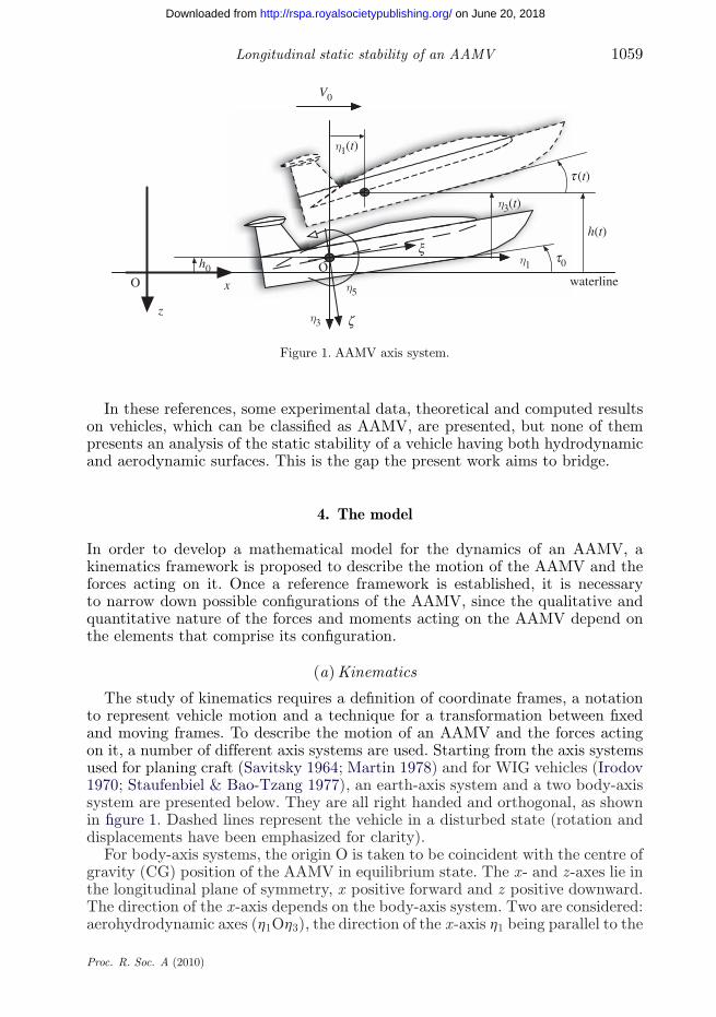
Figure 1. AAMV axis system.

In these references, some experimental data, theoretical and computed resultson vehicles, which can be classified as AAMV, are presented, but none of thempresents an analysis of the static stability of a vehicle having both hydrodynamicand aerodynamic surfaces. This is the gap the present work aims to bridge.

4. The model

In order to develop a mathematical model for the dynamics of an AAMV, akinematics framework is proposed to describe the motion of the AAMV and theforces acting on it. Once a reference framework is established, it is necessaryto narrow down possible configurations of the AAMV, since the qualitative andquantitative nature of the forces and moments acting on the AAMV depend onthe elements that comprise its configuration.

(a) Kinematics

The study of kinematics requires a definition of coordinate frames, a notationto represent vehicle motion and a technique for a transformation between fixedand moving frames. To describe the motion of an AAMV and the forces actingon it, a number of different axis systems are used. Starting from the axis systemsused for planing craft (Savitsky 1964; Martin 1978) and for WIG vehicles (Irodov1970; Staufenbiel & Bao-Tzang 1977), an earth-axis system and a two body-axissystem are presented below. They are all right handed and orthogonal, as shownin figure 1. Dashed lines represent the vehicle in a disturbed state (rotation anddisplacements have been emphasized for clarity).

For body-axis systems, the origin O is taken to be coincident with the centre ofgravity (CG) position of the AAMV in equilibrium state. The x- and z-axes lie inthe longitudinal plane of symmetry, x positive forward and z positive downward.The direction of the x-axis depends on the body-axis system. Two are considered:aerohydrodynamic axes (η1Oη3), the direction of the x-axis η1 being parallel to the





hydropropulsionsystem

main aerodynamicsurface

aeropropulsionsystem

secondary aerodynamicsurface

hydrodynamic surface

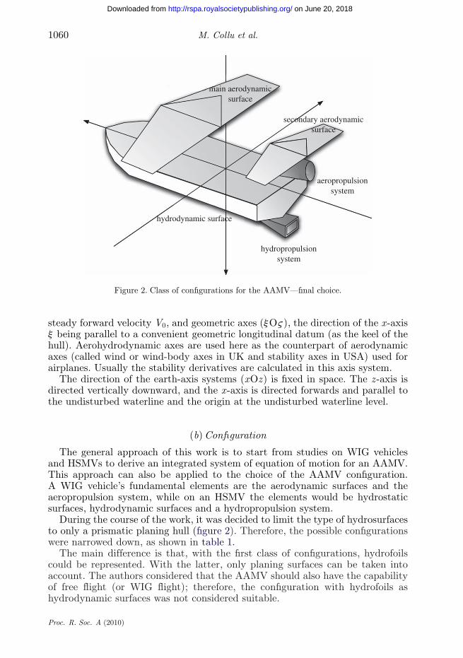
Figure 2. Class of configurations for the AAMV—final choice.

steady forward velocity V0, and geometric axes (ξOς), the direction of the x-axisξ being parallel to a convenient geometric longitudinal datum (as the keel of thehull). Aerohydrodynamic axes are used here as the counterpart of aerodynamicaxes (called wind or wind-body axes in UK and stability axes in USA) used forairplanes. Usually the stability derivatives are calculated in this axis system.

The direction of the earth-axis systems (xOz) is fixed in space. The z-axis isdirected vertically downward, and the x-axis is directed forwards and parallel tothe undisturbed waterline and the origin at the undisturbed waterline level.

(b) Configuration

The general approach of this work is to start from studies on WIG vehiclesand HSMVs to derive an integrated system of equation of motion for an AAMV.This approach can also be applied to the choice of the AAMV configuration.A WIG vehicle’s fundamental elements are the aerodynamic surfaces and theaeropropulsion system, while on an HSMV the elements would be hydrostaticsurfaces, hydrodynamic surfaces and a hydropropulsion system.

During the course of the work, it was decided to limit the type of hydrosurfacesto only a prismatic planing hull (figure 2). Therefore, the possible configurationswere narrowed down, as shown in table 1.

The main difference is that, with the first class of configurations, hydrofoilscould be represented. With the latter, only planing surfaces can be taken intoaccount. The authors considered that the AAMV should also have the capabilityof free flight (or WIG flight); therefore, the configuration with hydrofoils ashydrodynamic surfaces was not considered suitable.





Table 1. AAMV configuration elements.

element number note

aerodynamic surface 2 with/out control surfaceshydrodynamic surface 1 with/out control surfaces,

prismatic planing hullpropulsion system 1/more aero- and/or hydropropulsion system

Table 2. Forces and moments acting on an AAMV.

force symbol acting on

gravitational W centre of gravityhydrostatic and hydrodynamic N , Dws , DF hullaerodynamic Lai , Dai , aerodynamic surfaces

Mai , Dahaerodynamic and hydrodynamic aerodynamic surfacescontrol systems and hull (control fixed analysis,

are supposed constant, see §4d)aero- and/or hydropropulsion T thrust point

Among all the other possible hydrostatic/hydrodynamic surfaces, a prismaticplaning hull has been chosen, and the Savitsky planing hull model is used for thisconfiguration (Savitsky 1964). The available literature on planing craft dynamicsis extensive (Blake & Wilson 2001), and the approaches used are somewhat similarto the approach used for WIG vehicles: this aspect makes the coupling of theairborne and waterborne dynamics simpler. Also, if the majority of planing hullsused are non-prismatic, it has been demonstrated that the Savitsky approach issuitable also for non-prismatic hulls (Savitsky et al. 2007), and in particular inthe preliminary phase of design. To estimate the equilibrium state, the startingpoint of the static and dynamic stability analysis presented in this work, theSavitsky method is chosen, and along with it the prismatic planing monohullas the hydrostatic/hydrodynamic surface of the AAMV. The equilibrium stateestimation method has been previously developed by the authors (Collu 2008;Collu et al. 2008).

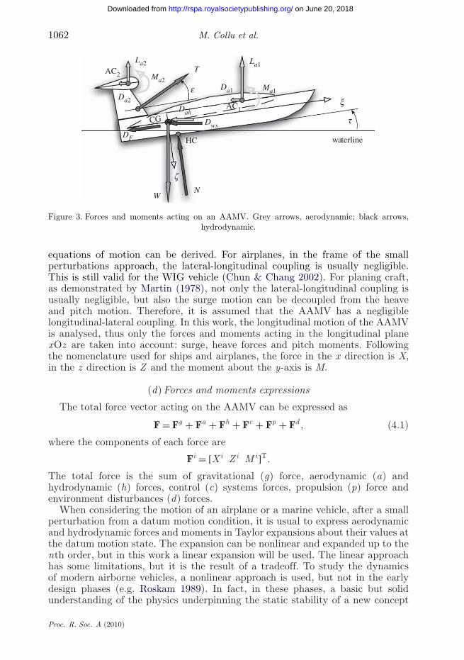
(c) Forces and moments acting on the aerodynamically alleviated marine vehicles

The forces and moments acting on the vehicle, after an external disturbance,are listed in table 2 and illustrated in figure 3.

(i) Decoupling of equations of motion

The AAMV, represented as a rigid body in space, and with control surfacesfixed, has six degrees of freedom. To describe its motion, a set of six simultaneousdifferential equations of motion is needed. However, a decoupled system of





waterline

x

z

CG t

HC

AC2

La1

Da1 Ma1

T

N

Da2

La2

e

W

DF

Dws

Ma2

AC1Dah

Figure 3. Forces and moments acting on an AAMV. Grey arrows, aerodynamic; black arrows,hydrodynamic.

equations of motion can be derived. For airplanes, in the frame of the smallperturbations approach, the lateral-longitudinal coupling is usually negligible.This is still valid for the WIG vehicle (Chun & Chang 2002). For planing craft,as demonstrated by Martin (1978), not only the lateral-longitudinal coupling isusually negligible, but also the surge motion can be decoupled from the heaveand pitch motion. Therefore, it is assumed that the AAMV has a negligiblelongitudinal-lateral coupling. In this work, the longitudinal motion of the AAMVis analysed, thus only the forces and moments acting in the longitudinal planexOz are taken into account: surge, heave forces and pitch moments. Followingthe nomenclature used for ships and airplanes, the force in the x direction is X,in the z direction is Z and the moment about the y-axis is M.

(d) Forces and moments expressions

The total force vector acting on the AAMV can be expressed as

F = Fg + Fa + Fh + Fc + Fp + Fd , (4.1)

where the components of each force are

Fi = [Xi Z i M i]T.

The total force is the sum of gravitational (g) force, aerodynamic (a) andhydrodynamic (h) forces, control (c) systems forces, propulsion (p) force andenvironment disturbances (d) forces.

When considering the motion of an airplane or a marine vehicle, after a smallperturbation from a datum motion condition, it is usual to express aerodynamicand hydrodynamic forces and moments in Taylor expansions about their values atthe datum motion state. The expansion can be nonlinear and expanded up to thenth order, but in this work a linear expansion will be used. The linear approachhas some limitations, but it is the result of a tradeoff. To study the dynamicsof modern airborne vehicles, a nonlinear approach is used, but not in the earlydesign phases (e.g. Roskam 1989). In fact, in these phases, a basic but solidunderstanding of the physics underpinning the static stability of a new concept





vehicle is needed, and the linear approach is perfect for this task. The nonlinearapproach would unnecessarily complicate the approach, hiding important aspectsand giving too detailed information at this stage. As regards hydrodynamicderivatives, linear methods are generally considered good enough to estimatethe static stability boundaries (Troesch & Falzarano 1993; Hicks et al. 1995).

As for airplanes and planing craft, forces and moments are assumed to dependon the values of the state variables and their derivatives with respect to time.Then, each force and moment is the sum of its value during the equilibrium stateplus its expansion to take into account the variation after a small disturbance,which is

F = F0 + F′,

F0 = [X0 Z0 M0]Tand F′ = [X ′ Z ′ M ′]T,

⎫⎪⎬⎪⎭ (4.2)

where the subscript (0) denotes starting equilibrium state and superscript (′)denotes perturbation from the datum. Initially, the AAMV is assumed tomaintain a rectilinear uniform level motion (RULM) with zero roll, pitch andyaw angles. In this particular motion, the steady forward velocity of the AAMVis V0 and its components in the aerohydrodynamic axis system are [η̇1,0, η̇3,0],with η̇1,0 = V0 and η̇3,0 = 0, since this is a level motion (constant height abovethe surface).

(i) Control, power and disturbances forces

In this analysis, it is assumed that the controls are fixed (similar to the ‘fixedstick analysis’ for airplanes). Then control forces and moment variations are equalto zero. The thrust is assumed not to vary during the small perturbation motion,and it is equal to the total drag of the vehicle. The effects of environmentaldisturbances, like waves, are beyond the scope of this work; so a stableundisturbed environment is assumed.

Fc = Fc0,

Fp = Fp0

and Fd = 0.

⎫⎪⎬⎪⎭ (4.3)

(ii) Gravitational force

The gravitational contribution to the total force can be obtained by resolvingthe AAMV weight into the body-axis system. Since the origin of the axis systemis coincident with the CG of the AAMV, there is no weight moment about they-axis. Remembering that the equilibrium state pitch angle is equal to zero andthe pitch angular perturbation θ ′ is small, the gravitational contribution is

Fg = Fg0 + Fg ′

,

Fg0 = [0 mg 0]T

and Fg ′ = [−mgθ ′ 0 0]T.

⎫⎪⎪⎬⎪⎪⎭ (4.4)





(iii) Aerodynamic forces

Usually, to evaluate aerodynamic forces and moments, the state variables takeninto account in their Taylor linear expansion are the velocity along the x andz-axes (η̇1 and η̇3) and the angular velocity about the y-axis (η̇5). Among theaccelerations, only the vertical acceleration (η̈3) is taken into account in the linearexpansion. Since the dynamics of a vehicle flying IGE depends also on the heightabove the surface, Kumar (1968a,b), Irodov (1970) and Staufenbiel & Bao-Tzang(1977) introduced for WIG vehicles the derivatives with respect to height (h).

These derivatives can be evaluated knowing the geometrical and aerodynamicscharacteristics of the aerodynamic surfaces of the AAMV (Hall 1994). As shownby Chun & Chang (2002), the Taylor expansion to first order (linear model) isa good approach to have a first evaluation of the static and dynamic stabilitycharacteristics of the WIG vehicle.

The expansion of the generic aerodynamic force (moment) in theaerohydrodynamic axis system (η1Oη3) for an AAMV with a longitudinal planeof symmetry is

Fa = Fa0 + Fa′

,

Fa0 = [Xa

0 Za0 Ma

0 ]T

and Fa′ =⎡⎢⎣

Xah

Zah

Mah

⎤⎥⎦ h ′ +

⎡⎢⎣

Xaη̇1

Xaη̇3

Xaη̇5

Zaη̇1

Zaη̇3

Zaη̇5

Maη̇1

Maη̇3

Maη̇5

⎤⎥⎦

⎡⎢⎣

η̇1

η̇3

η̇5

⎤⎥⎦

′

+⎡⎢⎣

0 Xaη̈3

0

0 Zaη̈3

0

0 Maη̈3

0

⎤⎥⎦

⎡⎢⎣

η̈1

η̈3

η̈5

⎤⎥⎦

′

.

⎫⎪⎪⎪⎪⎪⎪⎪⎬⎪⎪⎪⎪⎪⎪⎪⎭

(4.5)

The superscript a denotes aerodynamic forces. Fj denotes the derivative of theforce (or moment) F with respect to the state variable j ; it corresponds to thepartial differential ∂F/∂j .

(iv) Hydrodynamic forces

In Hicks et al. (1995), the nonlinear integro-differential expressions to calculatehydrodynamic forces and moments are expanded in a Taylor series, to third order.Therefore, equations of motion can be written as a set of ordinary differentialequations with constant coefficients. The planing craft dynamics are highlynonlinear, but the first step is to linearize the nonlinear system of equationsof motion and to calculate eigenvalues and eigenvectors, where variations aremonitored with quasi-static changes of physical parameters, such as the positionof the CG. This approach seems reasonable as a first step for the analysis of theAAMV dynamics too, for which a linear system of equations is developed.

The derivatives are usually divided into restoring coefficients (derivativeswith respect to heave displacement and pitch rotation), damping coefficients(derivatives with respect to linear and angular velocities) and addedmass coefficients (derivatives with respect to linear and angular accelerations).Martin (1978) and Troesch & Falzarano (1993) showed that the added massand damping coefficients are nonlinear functions of the motion, but also thattheir nonlinearities are small compared with the restoring forces nonlinearities:therefore, added mass and damping coefficients are assumed to be constant at agiven equilibrium motion. Their value can be extrapolated from experimental





results obtained by Troesch (1992). For the restoring coefficients, the linearapproximation presented in Troesch & Falzarano (1993) will be followed:

Fh,restoring − Fh,restoring0

∼= −[C ]η. (4.6)

The coefficients of [C ] can be determined using Savitsky’s method for a prismaticplaning hull (Savitsky 1964) or the approach presented by Faltinsen (2005).

An approach to estimate added mass, damping and restoring coefficients ispresented by Martin (1978). Furthermore, an alternative approach is to computethe added mass and damping coefficients as presented in Faltinsen (2005).

Then the expansion of the generic hydrodynamic force (moment) with respectto the aerohydrodynamic axis system η1Oη3 is

Fh = Fh0 + Fh ′

,

Fh0 = [

Xh0 Zh

0 Mh0

]T

and Fh ′ =⎡⎢⎣

0 Xhη3

Xhη5

0 Zhη3

Zhη5

0 Mhη3

Mhη5

⎤⎥⎦

⎡⎢⎣

η1

η3

η5

⎤⎥⎦

′

+⎡⎢⎣

Xhη̇1

Xhη̇3

Xhη̇5

Zhη̇1

Zhη̇3

Zhη̇5

Mhη̇1

Mhη̇3

Mhη̇5

⎤⎥⎦

⎡⎢⎣

η̇1

η̇3

η̇5

⎤⎥⎦

′

+⎡⎢⎣

Xhη̈1

Xhη̈3

Xhη̈5

Zhη̈1

Zhη̈3

Zhη̈5

Mhη̈1

Mhη̈3

Mhη̈5

⎤⎥⎦

⎡⎢⎣

η̈1

η̈3

η̈5

⎤⎥⎦

′

.

⎫⎪⎪⎪⎪⎪⎪⎪⎪⎪⎪⎪⎪⎪⎪⎪⎪⎬⎪⎪⎪⎪⎪⎪⎪⎪⎪⎪⎪⎪⎪⎪⎪⎪⎭

(4.7)

The superscript h denotes hydrodynamic forces. Xη1 , Zη1 and Mη1 are equalto zero since surge, heave and pitch moments are not dependent on the surgeposition of the AAMV.

(v) Equilibrium state

The equilibrium state has been already analysed (Collu 2008; Collu et al. 2008):here it is only briefly presented to make the necessary simplifications.

When an equilibrium state has been reached, by definition, all the accelerationsare zero as well as all the perturbation velocities and the perturbation forces andmoments. Then, using equations (4.3)–(4.5) and (4.7) in equation (4.2),

0 = Xa0 + Xh

0 + Xc0 + Xp

0 ,

0 = mg + Za0 + Zh

0 + Zc0 + Zp

0

and 0 = Ma0 + Mh

0 + Mc0 + Mp

0 .

⎫⎪⎪⎬⎪⎪⎭ (4.8)

(e) System of equations of motion

The generalized system of equations of motion (in six degrees of freedom) of arigid body with a left/right (port/starboard) symmetry is linearized in the frameof small-disturbance stability theory. The starting equilibrium state is an RULM,with a steady forward velocity equal to V0. The total velocity components of the





AAMV in the disturbed motion are (evaluated in the earth-axis system)⎡⎢⎢⎢⎢⎢⎢⎣

η̇1

η̇2

η̇3

η̇4

η̇5

η̇6

⎤⎥⎥⎥⎥⎥⎥⎦

=

⎡⎢⎢⎢⎢⎢⎢⎣

V0 + η̇′1

η̇′2

η̇′3

η̇′4

η̇′5

η̇′6

⎤⎥⎥⎥⎥⎥⎥⎦

. (4.9)

By definition for small disturbances, all the linear and the angular disturbancevelocities (denoted with a prime) are small quantities; therefore, substitutingequation (4.9) in the generalized six degrees of freedom equations of motion,and eliminating the negligible terms, the linearized equations of motion can beexpressed as

mη̈′1 = X ,

m(η̈′2 + η̇′

6V0) = Y ,

m(η̈′3 − η̇′

5V0) = Z ,

I44η̈′4 − I46η̈

′6 = L,

I55η̈′5 = M

and I66η̈′6 − I64η̈

′4 = N .

⎫⎪⎪⎪⎪⎪⎪⎪⎪⎪⎬⎪⎪⎪⎪⎪⎪⎪⎪⎪⎭

(4.10)

If the system of equations is decoupled, the longitudinal (symmetric) linearizedequations of motion are

mη̈′1 = X ,

m(η̈′3 − η̇′

5V0) = Z

and I55η̈′5 = M .

⎫⎪⎬⎪⎭ (4.11)

(f ) Longitudinal linearized system of equations of motion

Taking into account equation (4.8), the longitudinal linearized equations ofmotion (equation (4.11)) written in the aerohydrodynamic axis system can berearranged as

[A]η̈ + [B] η̇ + [C ] η + [D]h = 0, (4.12)

where

η =[η1η3η5

],

and h is the (perturbated) height above the waterline.The matrix [A] is the sum of the mass matrix, the hydrodynamic added mass

derivatives and the aerodynamic ‘added mass’ terms (usually in aerodynamicsthey are referred to as simply ‘acceleration derivatives’), whereas in the





hydrodynamic case these terms are much more significant.

[A] =⎡⎢⎣

m − Xhη̈1

−Xaη̈3

− Xhη̈3

−Xhη̈5

−Zhη̈1

m − Zaη̈3

− Zhη̈3

−Zhη̈5

−Mhη̈1

−Maη̈3

− Mhη̈3

I55 − Mhη̈5

⎤⎥⎦. (4.13)

[B] is the damping matrix and is defined as

[B] =⎡⎢⎣

−Xaη̇1

− Xhη̇1

−Xaη̇3

− Xhη̇3

−Xaη̇5

− Xhη̇5

−Zaη̇1

− Zhη̇1

−Zaη̇3

− Zhη̇3

−Zaη̇5

− Zhη̇5

−Maη̇1

− Mhη̇1

−Maη̇3

− Mhη̇3

−Maη̇5

− Mhη̇5

⎤⎥⎦. (4.14)

[C ] is the restoring matrix and is defined as

[C ] =⎡⎢⎣

0 −Xhη3

−mg − Xhη5

0 −Zhη3

−Zhη5

0 −Mhη3

−Mhη5

⎤⎥⎦. (4.15)

The matrix [D] represents the WIG, to take into account the influence of theheight above the surface on the aerodynamic forces:

[D] =⎡⎢⎣

−Xah

−Zah

−Mah

⎤⎥⎦. (4.16)

(g) Cauchy standard form of the equations of motion

By defining a state-space vector ν as

ν = [η̇1 η̇3 η̇5 η3 η5 η0]T (4.17)

the system of equations (equation (4.12)) can be transformed to the Cauchystandard form (or state-space form). The state-space vector has six variableswhile the system of equations (equation (4.12)) has only three equations. Theremaining three equations are

∂(η3)∂t

= η̇3,

∂(η5)∂t

= η̇5

and∂(h)∂t

= ∂(η0)∂t

= −η̇3 + V0η5.

⎫⎪⎪⎪⎪⎪⎪⎬⎪⎪⎪⎪⎪⎪⎭

(4.18)

Therefore, the system is

[ASS]ν̇ = [BSS]ν, (4.19)





where

[ASS] =

⎡⎢⎢⎣

[A] [0]3×3

[0]3×3

1 0 00 1 00 0 1

⎤⎥⎥⎦ (4.20)

and

[BSS] =

⎡⎢⎢⎢⎢⎢⎢⎣

−[B]0 −mg

−C33 −C35−C53 −C55

−[D]

0 1 0 0 0 00 0 1 0 0 00 −1 0 0 V0 0

⎤⎥⎥⎥⎥⎥⎥⎦

. (4.21)

The system of equations of motion in a state-space form is

ν̇ = [H ] ν, (4.22)

where[H ] = [ASS]−1 [BSS]. (4.23)

Now it is possible to analyse the static and dynamic stability of an AAMVconfiguration, and the influence of the configuration characteristics on the AAMVdynamics.

5. Static stability

Analysing the forces and moments under the small-disturbance hypothesis, thestatic stability of an AAMV is derived using the Routh–Hurwitz criterion.

In particular, Staufenbiel & Bao-Tzang (1977) showed how the last coefficientA0 of the characteristic polynomial of a WIG vehicle can be used to estimate itsstatic stability. In general, given the characteristic polynomial of a system

Ansn + An−1sn−1 + · · · + A1s1 + A0 = 0, (5.1)

if the conditionA0

An> 0 (5.2)

with An > 0, is fulfilled, the system is statically stable.

(a) Characteristic polynomial and static stability condition foraerodynamically alleviated marine vehicles

In §4, the mathematical model is developed to study the longitudinal dynamicsof an AAMV. A system of ordinary differential equations of motion is derived forthe longitudinal plane in the frame of small-disturbance stability theory. Startingfrom this model, the Routh–Hurwitz condition is used to derive a mathematicalexpression to estimate the AAMV static stability.





(i) Complete order system

By defining a state-space vector ν as

ν = [η̇1 η̇3 η̇5 η3 η5 η0]T (5.3)

the system of equations of motion can be rearranged in the Cauchy standard form(or state-space form), showed in equation (4.19). The characteristic polynomialof the complete order system can be derived:

A6s6 + A5s5 + A4s4 + A3s3 + A2s2 + A1s1 + A0 = 0. (5.4)

With A6 = 1, the static stability is assured when

A0 = num0

�> 0, (5.5)

where num0 is equal to

num0 = V0[D10(B31 C53 − B51 C33) − B11(C35 D50 − C53 D30)] (5.6)

and � is equal to

� = (I55 + A55)[m2 + m(A11 + A33) + A11A33 − A31A13]− (m + A11)A53A35 − (m + A33)A51A15 + A53A31A15 + A51A13A35. (5.7)

Aij , Bij , Cij and Dij stability derivatives are illustrated, respectively, inequations (4.13)–(4.16).

(ii) Reduced order system

This mathematical method has to be validated against experimental data.Unfortunately, no experimental data on the static stability of an AAMVconfiguration are available in the public domain.

To plan experiments to obtain these data, it is necessary to have a physicalinsight of the condition stated in equation (5.2). This condition, applied to thecomplete order system in equation (5.5), is relatively complex. Assuming thatthe surge degree of freedom (η1) can be decoupled from heave (η3) and (η5) pitchdegrees of freedom, a simplified version of the condition in equation (5.5) can beobtained, leading to a better physical insight.

The mathematical model of the dynamics developed here starts from thesystems of equations of motion for WIG vehicles and planing craft. As regards thedynamics of a planing craft, Martin (1978) demonstrated that the surge motioncan be decoupled from the heave and pitch motion. For the dynamics of WIGvehicles, Rozhdestvensky (1996) proposed a reduced order system where the surgemotion is decoupled from heave and pitch motion.

By defining the reduced order state-space vector ν as

ν = [η̇3 η̇5 η3 η5 η0]T , (5.8)

the Cauchy standard form (or state-space form) of the reduced order system isobtained. The characteristic polynomial can be derived:

A5s5 + A4s4 + A3s3 + A2s2 + A1s1 + A0 = 0. (5.9)




a


With A5 = 1, the static stability is assured when

A0 = V0(C33 D50 − C53D30)(A55 + I55)(A3 + m) − A53A35

> 0. (5.10)

(b) Reduced order static stability: physical insight

Each coefficient in equation (5.10) is the derivative with respect to accelerations(Aij), heave position (Cij) and height above the surface (Dij) of the sumof aerodynamic and hydrodynamic forces (and moments). Referring to §4f ,remembering that the superscript ‘a’ stands for aerodynamic and ‘h’ forhydrodynamic, and that Z is the heave force (positive downward) and M thepitch moment (positive bow-up), the coefficients are equal to

A33 = Aa33 + Ah

33 = −Zaη̈3 − Zh

η̈3,

A35 = Aa35 + Ah

35 = −Zaη̈5 − Zh

η̈5,

A53 = Aa53 + Ah

53 = −Maη̈3 − Mh

η̈3

and A55 = Aa55 + Ah

55 = −Maη̈5 − Mh

η̈5.

⎫⎪⎪⎪⎪⎪⎪⎬⎪⎪⎪⎪⎪⎪⎭

(5.11)

C33 = Ch33 = −Zh

η3, Ca33 = 0,

C53 = Ch53 = −Mh

η3, Ca53 = 0,

D30 = Da30 = −Za

η0, Dh30 = 0,

nd D50 = Da53 = −Ma

η0, Dh50 = 0.

⎫⎪⎪⎪⎪⎪⎬⎪⎪⎪⎪⎪⎭

(5.12)

The aerodynamic derivatives can be estimated with the approach presentedin Hall (1994) and the hydrodynamic derivatives with expressions presentedby Martin (1978) and by Faltinsen (2005). Using these expressions for theconfiguration presented in §4b, we have

(A55 + I55)(m + A33) − A53 A35 > 0; (5.13)

therefore, since the denominator of equation (5.10) is greater than zero, the staticstability condition of the reduced order becomes

D50

D30− C53

C33> 0. (5.14)

(i) Similarity with wing in ground effect vehicles

To better understand the condition expressed in equation (5.14), a parallel withWIG vehicles static stability criteria is illustrated. The static stability conditionderived by Staufenbiel & Bao-Tzang (1977) and Irodov (1970) is

Mw

Zw− Mh

Zh< 0, (5.15)

which, using the present nomenclature, corresponds to the conditionB53

B33− D50

D30< 0. (5.16)





Mw and Mh are the derivatives of pitch moment with respect to, respectively,the heave velocity and the height above the surface, Zw and Zh are the heaveforce same derivatives. Staufenbiel & Bao-Tzang (1977) and Irodov (1970) defineMw/Zw also as the aerodynamic centre of pitch and Mh/Zh as the aerodynamiccentre in height. Remembering that positive abscissa means ahead of the CG, thecondition in equations (5.15) and (5.16) can be expressed as:

the (aerodynamic) centre in height should be located upstream of the(aerodynamic) centre in pitch.

(Rozhdestvensky 2006, p. 243)

Dividing the lift owing to a variation of the pitch angle (�Lalpha) from the liftowing to a variation of the height above the surface (�Lheight), the condition inequation (5.15) states that the point of action of force �Lheight should be locatedupstream of the point of action of force �Lalpha.

(ii) Aerodynamically alleviated marine vehicle static stability criterion (reducedorder)

As regards the AAMV, using expressions (5.12), the static stability conditionin equation (5.14) can be expressed as

Maη0

Zaη0

− Mhη3

Zhη3

> 0. (5.17)

The first term Maη0/Z

aη0 is the analogue of the aerodynamic centre in height of

WIG vehicles. The authors propose for the second term the name ‘hydrodynamiccentre in heave’, so that equation (5.17) can also be expressed as:

the hydrodynamic centre in heave should be located downstream of theaerodynamic centre in height.

As before, dividing the hydrodynamic lift owing to a heave variation (�Lhyd)from the lift owing to a variation of the height above the surface (�Lheight), itneeds to be checked that the point of action of �Lhyd is located upstream of thepoint of action of �Lhyd.

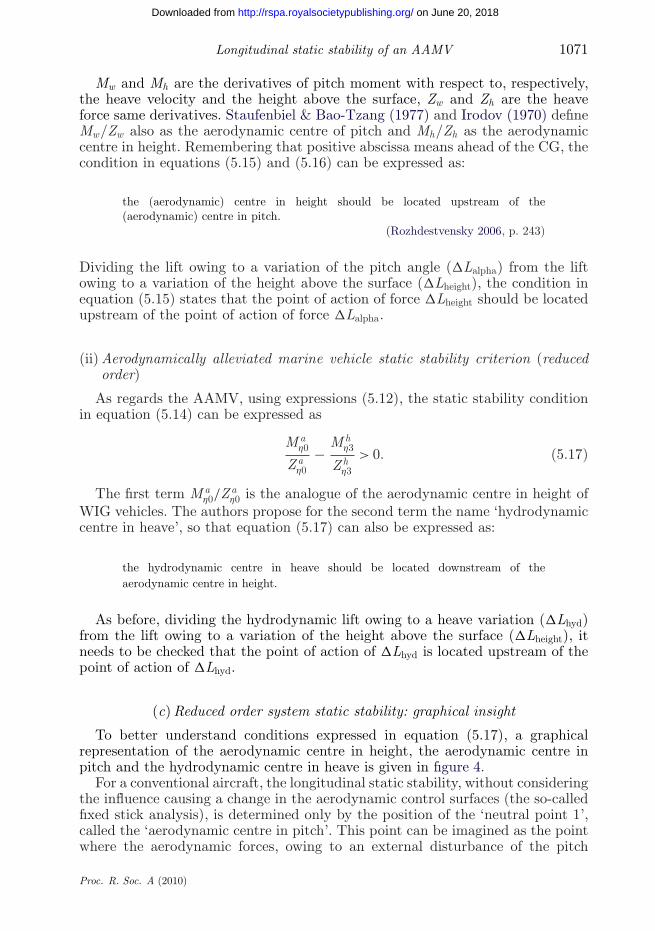
(c) Reduced order system static stability: graphical insight

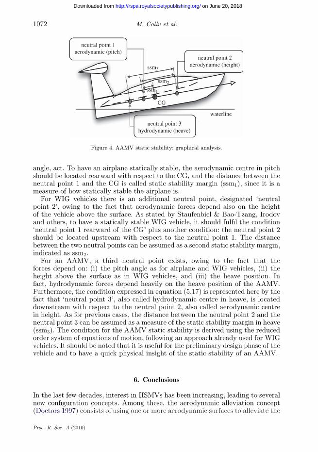
To better understand conditions expressed in equation (5.17), a graphicalrepresentation of the aerodynamic centre in height, the aerodynamic centre inpitch and the hydrodynamic centre in heave is given in figure 4.

For a conventional aircraft, the longitudinal static stability, without consideringthe influence causing a change in the aerodynamic control surfaces (the so-calledfixed stick analysis), is determined only by the position of the ‘neutral point 1’,called the ‘aerodynamic centre in pitch’. This point can be imagined as the pointwhere the aerodynamic forces, owing to an external disturbance of the pitch





neutral point 1aerodynamic (pitch)

neutral point 2aerodynamic (height)

neutral point 3hydrodynamic (heave)

ssm3

ssm2

ssm1

CG

waterline

Figure 4. AAMV static stability: graphical analysis.

angle, act. To have an airplane statically stable, the aerodynamic centre in pitchshould be located rearward with respect to the CG, and the distance between theneutral point 1 and the CG is called static stability margin (ssm1), since it is ameasure of how statically stable the airplane is.

For WIG vehicles there is an additional neutral point, designated ‘neutralpoint 2’, owing to the fact that aerodynamic forces depend also on the heightof the vehicle above the surface. As stated by Staufenbiel & Bao-Tzang, Irodovand others, to have a statically stable WIG vehicle, it should fulfil the condition‘neutral point 1 rearward of the CG’ plus another condition: the neutral point 2should be located upstream with respect to the neutral point 1. The distancebetween the two neutral points can be assumed as a second static stability margin,indicated as ssm2.

For an AAMV, a third neutral point exists, owing to the fact that theforces depend on: (i) the pitch angle as for airplane and WIG vehicles, (ii) theheight above the surface as in WIG vehicles, and (iii) the heave position. Infact, hydrodynamic forces depend heavily on the heave position of the AAMV.Furthermore, the condition expressed in equation (5.17) is represented here by thefact that ‘neutral point 3’, also called hydrodynamic centre in heave, is locateddownstream with respect to the neutral point 2, also called aerodynamic centrein height. As for previous cases, the distance between the neutral point 2 and theneutral point 3 can be assumed as a measure of the static stability margin in heave(ssm3). The condition for the AAMV static stability is derived using the reducedorder system of equations of motion, following an approach already used for WIGvehicles. It should be noted that it is useful for the preliminary design phase of thevehicle and to have a quick physical insight of the static stability of an AAMV.

6. Conclusions

In the last few decades, interest in HSMVs has been increasing, leading to severalnew configuration concepts. Among these, the aerodynamic alleviation concept(Doctors 1997) consists of using one or more aerodynamic surfaces to alleviate the





Table 3. Comparison between the dynamics characteristics of conventional configurations andthe AAMV dynamics. SPPO, short period pitch oscillation.

vehicle system ofconfiguration equations of motion roots

airplane four equations two oscillatory solutions:∂x/∂t, ∂z/∂t, ∂θ/∂t, θ phugoid, SPPO

planing craft four equations two oscillatory solutions:∂z/∂t, z , ∂θ/∂t, θ porposing (least stable root)

WIG vehicles five equations two oscillatory solutions, 1 real root:∂x/∂t, ∂z/∂t, ∂θ/∂t, θ , h phugoid, SPPO, subsidence mode

AAMV six equations for the reduced-order system,∂x/∂t, ∂z/∂t, z , without ∂x/∂t,∂θ/∂t, θ , h two oscillatory solutions, one real root

weight of the marine vehicle. Basically, the advantages are: (i) a total drag, at highspeed, up to 20–30% lower than the same marine vehicle without aerodynamicsurfaces (Collu 2008), (ii) vertical and angular pitch accelerations, at high speed,30–60% lower than conventional HSMV (Kallio 1978), and (iii) a vehicle bridgingthe speed gap and payload gap between conventional HSMV and airplanes.

To classify this configuration concept, the new abbreviation AAMV,aerodynamically alleviated marine vehicle, is used. Being a relatively recentconfiguration concept, it lacks a specifically developed mathematical frameworkto study its dynamics. The AAMV experiences aerodynamic and hydrodynamicforces of the same order of magnitude, therefore the mathematical frameworksdeveloped separately so far for HSMVs and airplanes are not suitable. Thispaper presents an integrated mathematical framework specifically for an AAMVconfiguration.

(i) Aerodynamically alleviated marine vehicle system of equations of motion

A mathematical model of the longitudinal dynamics of an AAMVconfiguration, developed in the small-disturbance framework, is presented.Coupling the systems of equations of motion, available in the literature, used forWIG vehicles and for high-speed planing craft, the authors derived a new systemof equations of motion. This mathematical model takes into account aerodynamic,hydrodynamic and hydrostatic stability derivatives, leading to a new dynamics.In fact, also if this AAMV mathematical model is obtained by combining the WIGvehicles and the planing craft dynamics, the resultant dynamics is not simply thesum of these dynamics. As shown in table 3, the system of equations of motiondeveloped by the authors proposes a new dynamic feature, with a potential newmode of oscillation and a more complex dynamics with respect to WIG vehicles,planing craft and conventional airplanes.

(ii) Static stability criterion of aerodynamically alleviated marine vehicles

The AAMV dynamics differ substantially from planing craft dynamics andfrom airplanes and WIG vehicles dynamics, and the static stability of an AAMVconfiguration is analysed, and a new static stability criterion is proposed.





Briefly, in the longitudinal plane, airplanes possess one neutral point, calledthe aerodynamic neutral point in pitch (or also neutral point): if this point isrearward with respect to the CG of the vehicle, the airplane is statically stable.By contrast, WIG vehicles have an additional neutral point, the aerodynamicneutral point in height, owing to the fact that aerodynamic forces depend alsoon the vehicle’s height above the surface. To have a WIG vehicle statically stablein height, this second neutral point should be upstream with respect to the firstneutral point, as investigated by Staufenbiel & Bao-Tzang (1977), Irodov (1970)and Rozhdestvensky (1996). For an AAMV, a third neutral point exists, owingto the fact that the forces depend on the pitch angle, as for an airplane and WIGvehicles, the height above the surface, as in WIG vehicles, and the heave position.In fact, the hydrodynamic forces depend heavily on the heave position of theAAMV. The condition expressed by equation (5.17) can be expressed saying thatthe third neutral point, also called the hydrodynamic centre in heave, should belocated downstream with respect to the neutral point 2 to have an AAMV that isstatically stable in heave. The relative position of each point is shown in figure 4.In airplane dynamics, the distance between the CG and the (aerodynamic) neutralpoint (in pitch) is called the static stability margin (ssm1). Following the sameapproach, the distance between the second neutral point and the first neutralpoint can be called the static stability margin in height (ssm2). As already said,for an AAMV configuration a third neutral point exists, and the distance betweenthe second and the third neutral point can be called the hydrodynamic staticstability margin in heave (ssm3).

References

Blake, J. I. R. & Wilson, P. A. 2001 A visual experimental technique for planing craft performance.Trans. R. Inst. Naval Architects 143, 393–404.

Bryan, G. H. & Williams, W. E. 1904 The longitudinal stability of aerial gliders. Proc. R. Soc.Lond. 73, 100–116. (doi:10.1098/rspl.1904.0017)

Chun, H. H. & Chang, C. H. 2002 Longitudinal stability and dynamic motion of a small passengerWIG craft. Ocean Eng. 29, 1145–1162.

Clark, D. J., Ellsworth, W. M. & Meyer, J. R. 2004 The quest for speed at sea. Technical Digest,Naval Surface Warfare Center, Carderock Division.

Collu, M. 2008 Marine vehicles with aerodynamic surfaces: dynamics mathematical modeldevelopment. PhD thesis, Cranfield University, Cranfield.

Collu, M., Patel, M. H. & Trarieux, F. 2008 A mathematical model to analyse the static stability ofhybrid (aero-hydrodynamically supported) vehicles. 8th Symp. on High Speed Marine Vehicles,Naples, Italy, 21 May 2008, pp. 148–161.

Doctors, L. J. 1997 Analysis of the efficiency of an ekranocat: a very high speed catamaran withaerodynamic alleviation. Int. Conf. on Wing in Ground Effect Craft, London, UK, 4 December1997.

Faltinsen, O. M. 2005 Hydrodynamics of high-speed vehicles, p. 454. Cambridge, UK: CambridgeUniversity Press.

Hall, I. A. 1994 An investigation into the flight dynamics of wing in ground effect aircraft operatingin aerodynamic flight. MSc thesis, Cranfield University, Cranfield.

Hicks, J. D., Troesch, A. W. & Jiang, C. 1995 Simulation and nonlinear dynamics analysis ofplaning hulls. J. Offshore Mech. Arch. Eng. 117, 38–45. (doi:10.1115/1.2826989)

Irodov, R. D. 1970 Kriterii prodol’noy ustoychivosti ekranoplana. TsAGI im. N. Ye. Zhukovskij 1,63–72. (Transl. WIG longitudinal stability criteria, Central Institute of Aerohydrodynamics).


http://dx.doi.org/doi:10.1098/rspl.1904.0017

http://dx.doi.org/doi:10.1115/1.2826989




Kallio, J. A. 1978 Results of full scale trials on two high speed planing craft (Kudu II and Kaama).Report no. DTNSRDC/SPD-0847-01, David W. Taylor Naval Ship Research and DevelopmentCenter, Carderock, MD.

Kolyzaev, B., Zhukov, V. & Maskalik, A. 2000 Ekranoplans, peculiarity of the theory and design.Saint Petersburg, Russia: Sudostroyeniye.

Kumar, P. 1968a Stability of ground effect vehicles. Report no. Aero 198, Cranfield College ofAeronautics.

Kumar, P. 1968b On the longitudinal dynamic stability of a ground effect wing. Report no. Aero202, Cranfield College of Aeronautics.

Martin, M. 1978 Theoretical determination of porpoising instability of high-speed planing boats.J. Ship Res. 22, 32–53.

Perring, W. G. A. & Glauert, H. 1932 Stability on the water of a seaplane in the planing condition.Reports and Memoranda no. 1493, Aeronautical Research Committee, London.

Roskam, J. 1989 Airplane design, part II: preliminary sizing of airplanes. Ottawa, Ontario: RoskamAviation and Engineering Corporation.

Rozhdestvensky, K. V. 1996 Ekranoplans—the GEM’s of fast water transport. Trans. Inst. Mar.Eng. 109, 47–74.

Rozhdestvensky, K. V. 2006 Wing-in-ground effect vehicles. Prog. Aerosp. Sci. 1, 211–283.(doi:10.1016/j.physletb.2003.10.071)

Savitsky, D. 1964 Hydrodynamic design of planing hulls. J. Mar. Technol. 1, 71–95.Savitsky, D., De Lorme, M. F. & Datla, R. 2007 Inclusion of whisker spray drag in performance

prediction method for high-speed planing hulls. Mar. Technol. 44, 35–56.Shipps, P. R. 1976 Hybrid ram-wing/planning craft—today’s raceboats, tomorrow’s outlook.

AIAA/SNAME Advanced Marine Vehicles Conf., Arlington, VA, 20 September 1976, pp. 1–8.Staufenbiel, R. W. & Bao-Tzang, Y. 1977 Stability and control of ground effect aircraft

in longitudinal motion. Report (translation), David W. Taylor Naval Ship Research andDevelopment Center.

Troesch, A. W. 1992 On the hydrodynamics of vertically oscillating planing hulls. J. Ship Res. 36,317–331.

Troesch, A. W. & Falzarano, J. W. 1993 Modern nonlinear dynamical analysis of vertical planemotion of planing hulls. J. Ship Res. 37, 189–199.

Ward, T. M., Goelzer, H. F. & Cook, P. M. 1978 Design and performance of the ram wing planingcraft—KUDU II. AIAA/SNAME Advanced Marine Vehicles Conf., San Diego, CA, 17 April1978, pp. 1–10.

Zarnick, E. E. 1978 A nonlinear mathematical model of motions of a planing boat in regular waves.Report no. DTNSRDC 78-032, David W. Taylor Naval Ship Research and Development Center,Carderock, MD.


http://dx.doi.org/doi:10.1016/j.physletb.2003.10.071


The longitudinal static stability of an aerodynamically...

Documents

Transcript of The longitudinal static stability of an aerodynamically...