.ro

rspa.royalsocietypublishing.org

ResearchCite this article: Jana P, Chatterjee A. 2013Modal damping in vibrating objects viadissipation from dispersed frictionalmicrocracks. Proc R Soc A 469: 20120685.http://dx.doi.org/10.1098/rspa.2012.0685

Received: 16 November 2012Accepted: 8 January 2013

Subject Areas:mechanical engineering

Keywords:vibration damping, internal dissipation,friction, microcrack, Monte Carlo,constitutive model

Author for correspondence:Prasun Janae-mail: prasunjana@gmail.com

†Present address: Mechanical Engineering,Indian Institute of Technology,Kanpur 208016, India.

Electronic supplementary material is availableat http://dx.doi.org/10.1098/rspa.2012.0685 orvia http://rspa.royalsocietypublishing.org.

http://rspaDownloaded from

Modal damping in vibratingobjects via dissipation fromdispersed frictionalmicrocracksPrasun Jana and Anindya Chatterjee†

Mechanical Engineering, Indian Institute of Technology,Kharagpur 721302, India

Many materials under multiaxial periodic loadingexhibit rate-independent internal dissipation percycle. Constitutive modelling for such dissipationunder spatially variable triaxial stresses is neededfor calculating modal damping of solid bodiesusing computational packages. Towards a micro-mechanically motivated model for such dissipation,this paper begins with a frictional microcrackin a linearly elastic solid under far-field time-periodic tractions. The material is assumed to containmany such non-interacting microcracks. Single-cracksimulations, in two and three dimensions, areconducted using ABAQUS. The net cyclic single-crack dissipation under arbitrary triaxial stresses isfound to match, up to one fitted constant, a formulabased on a pseudostatic spring-block model. Thatformula is used to average the energy dissipationfrom many randomly oriented microcracks usingMonte Carlo averaging. A multivariate polynomialis fitted to the Monte Carlo results. The polynomialis used in finite-element simulation of a solid object,wherein modal analysis is followed by computationof the net cyclic energy dissipation via elementwiseintegration. The net dissipation yields an equivalentmodal damping. In summary, starting from a knownformula for a single crack, this paper developsand implements a method for computationallymodelling the modal damping of arbitrarily shapedsolid bodies.

1. IntroductionThis work is motivated by an engineering designproblem. Consider two possible designs (shapes anddimensions) for some engineering component, to be

c© 2013 The Author(s) Published by the Royal Society. All rights reserved.

on September 21, 2018yalsocietypublishing.org/

2

rspa.royalsocietypublishing.orgProcRSocA469:20120685

..................................................

on September 21, 2018http://rspa.royalsocietypublishing.org/Downloaded from

1

XYZ

NOV 9 201213:48:44

ELEMENTS1

MN MX

XYZ

0.265E-050.007506

0.015010.022513

0.0300170.037521

0.0450240.052528

0.0600310.067535

NOV 9 201213:49:06

NODAL SOLUTIONSTEP = 1SUB =7FREQ = 121.587USUM (AVG)RSYS = SOLUDMX = 0.067535SMN = 0.265E-05SMX = 0.067535

(a) (b)

Figure 1. (a) FE model of an arbitrarily chosen object. (b) Its first vibration mode. (Online version in colour.)

made of some known, lightly dissipative material. Which design has better vibrationdamping?

A computational approach would begin with straightforward finite-element (FE)-based modalanalysis. It would also require a constitutive relation for material damping under time-periodictriaxial inhomogeneous stresses. As discussed below, such a relation is not presently available. Tofix ideas, consider the solid object of figure 1a, modelled using an FE package, with its first modeas shown in figure 1b. We seek a constitutive relation that can be used, along with modal analysis,to compute the damping ratios for the first several modes of such an object.

We begin by reviewing the relevant literature on internal damping. For many solids vibratingat low frequencies, it has been observed that internal energy dissipation (or material damping,or internal damping) per unit volume and per cycle of deformation is frequency independent andapproximately proportional to some power (n ≥ 2) of the stress amplitude. We write

Dm = Jσ neq, (1.1)

where Dm stands for specific material damping, σeq is a suitable stress amplitude, and J and nare fitted constants. Such frequency independence was reported by Lord Kelvin [1]. Rowett [2]studied torsion of steel tubes and observed frequency-independent power-law dissipation withn ≈ 3. Kimball & Lovell [3] found n ≈ 2 and frequency independence for 18 different materials,including metals, celluloid, glass, rubber and wood. Such frequency-independent power-lawbehaviour has been discussed by many others. Lazan [4] adopted a phenomenological approachand used power laws. Granato & Lücke [5] proposed an explanation based on dislocation pinningby impurity particles. Dawson [6] considered an unknown function of non-dimensionalizedstress, formally expanded in a Taylor series using even powers only, leading by assumption ton = 2 for small stresses.

However, as indicated above, we are interested in multiaxial stress states. No convincingmechanically based engineering model for the same is presently available. For example, theempirical laws in Lazan [4] do not identify the equivalent stress of equation (1.1) under anarbitrary triaxial load. Dislocation-based models as in Granato & Lücke [5] involve severalparameters related to the crystal structure, yet to be translated into measurable externalmacroscopic model parameters. The approach of Dawson [6] also does not identify the role ofmultiaxial stresses in the dissipation model. As a final example, Hooker [7] proposed that theequivalent stress amplitude should be computed as

σ 2eq = (1 − λ)(I2

1 − 3I2) + λI21; 0 < λ < 1, (1.2)

where I1 and I2 are the first and second stress invariants, respectively, and λ is a fitted parameter.The above is motivated by the fact that it is a linear combination of distorsional and dilatationalstrain energies.

3

rspa.royalsocietypublishing.orgProcRSocA469:20120685

..................................................

on September 21, 2018http://rspa.royalsocietypublishing.org/Downloaded from

In contrast to the above, there is in fact a micromechanical modelling approach that seemspromising for our purposes. This approach considers randomly distributed frictional microcrackswithin an elastic material, as opposed to the ad hoc prescription of equation (1.2).

The literature on frictional microcracks in elastic materials is rich. Kachanov [8] proposedan approximate analysis method based on a superposition principle for interactions of multiplecracks at moderate distances from each other. Aleshin & Abeele [9] presented a tensorial stress–strain hysteresis model due to friction in unconforming grain contacts. Their model pays closeattention to the variation of actual area of contact under normal stress, but has many parameters(seven for uniaxial compression alone). Deshpande & Evans [10] studied frictional microcracks inthe context of inelastic deformation and fracture of ceramics. Al-Rub & Palazotto [11] computedenergy dissipation in ceramic coatings and found that frictional dissipation in microcrackscontributes significantly to overall dissipation. More recently, Barber and co-workers havepresented several papers on mechanics with frictional microcracks. Jang & Barber [12] discussedthe dissipation in interacting microcracks using Kachanov’s [8] approach. Barber et al. [13] studieda single frictional elastic contact subjected to periodic loading. The contact has an extended area,part of which sticks while the remainder can slip; some basic results about energy dissipationunder periodic loading are obtained. Jang & Barber [14] examined the substantial effect of therelative phase of harmonically varying tangential and normal loads on the dissipation in anuncoupled frictional system. Barber [15] discussed discrete frictional systems under oscillatingloads, and examined the conditions under which the steady-state solution retains a memory ofthe initial state. Individual cracks with surface roughness models for the contacting faces havebeen studied by Putignano et al. [16], who observed that, with microslip in variable regions butno gross slip at the contact surfaces, energy dissipation varies as the cube of the stress amplitudefor small amplitudes.

None of the above studies have considered the net dissipation in a body, with spatiallyvariable stresses, from a multitude of randomly oriented frictional microcracks. Here, we seeka macroscopic constitutive relation for such dissipation.

To this end, for simplicity, we assume that the cracks are small and far apart (non-interacting);that initial super-small microslips on crack surface asperities can be neglected, and the crack facesmodelled as non-adhering yet geometrically flat; that all crack face frictions can be modelled usinga single coulomb friction coefficient μ; and that the material remains linearly elastic. We assumethat the normal and tangential loadings at each crack are in phase (as would occur for vibrationof a body in a single mode). Although our initial formulation allows both non-zero mean stressesand non-uniform distributions of crack face orientations, our final formula assumes zero meanstress and uniformly distributed crack face orientations.

Under these assumptions, we develop an empirical formula with two fitted parameters for thedissipation per unit volume and per cycle of time-periodic triaxial stress, and use the solid objectof figure 1a in a computational example.

The contribution of this paper may thus be viewed as the first assembly of the following tasksin one self-contained sequence: we use existing ideas about bodies with frictional microcracks,integrate their dissipation rate over all possible crack orientations, develop a constitutive modelfor the net specific dissipation per cycle, and demonstrate the use of the formula to compute themodal damping ratios of arbitrarily shaped objects.

2. Frictional dissipation in a single microcrackThe first step in our task is to compute the frictional dissipation in a single microcrack due toremote cyclic loading. For the two-dimensional case, an analytical treatment is given in Jang &Barber [12], including an analytical formula based on a single degree of freedom spring-blockmodel for when the entire crack face sticks or slips as one. We have studied the same using FEcalculations in both two and three dimensions. The formula based on the spring-block model,with one fitted constant, turns out to be highly accurate. These computations are outlined below(for details, see the electronic supplementary material).

4

rspa.royalsocietypublishing.orgProcRSocA469:20120685

..................................................

on September 21, 2018http://rspa.royalsocietypublishing.org/Downloaded from

xy

z

-sy

txy

–sz

-sx

tzy tzx

t

s

t

s(a) (b)

time

1 cycle

stre

ss compressive

tensile

sa ta

sm

frictionalcrack

(c)

Figure 2. (a) An element with a small embedded frictional crack. (b) Two-dimensional representation. (c) Applied normal andshear loads. Sign convention for mean normal stress: compression is positive. Solid blue line,σ ; dashed line, τ . (Online versionin colour.)

Look at figure 2a, where the crack is circular, planar and parallel to the horizontal faces of acube-shaped element. We have found in separate two-dimensional computations that removingtiny regions around the crack tips does not influence the net dissipation, and so material orgeometric nonlinearities are neglected.

We can simplify the three-dimensional picture. To any given state of stress and deformation,an additional σx causes an additional uniform strain in the element but no added shearing atthe crack face. Consequently, σx causes no slip and does not contribute to the energy dissipated.Similar arguments apply for σy and τxy. Thus σx, σy and τxy do not affect our results and aredropped. By contrast, σz will affect the frictional forces, while τzx and τzy will cause frictionalsliding. Finally, by rotating the coordinate system about the z-axis, τzx can be made zero. Thisleaves just the normal stress σz = σ and the shear component τzy = τ contributing to frictionaldissipation. A two-dimensional representation is shown in figure 2b.

Figure 2c depicts possible periodic normal and shear tractions, acting in phase, on theelement of interest. Inertia is negligible (alternatively, frequencies are low), so the dissipation isfrequency-independent. Our pseudostatic simulation results will actually apply to every periodicwaveform where (i) the changes in far-field normal and shear stresses maintain a fixed proportionthroughout the load cycle (i.e. the time-varying parts have similar waveforms) and (ii) there areonly two points of stress reversal per cycle. See the electronic supplementary material for somepossible waveforms. For convenience, we used a triangular loading pattern in our computationsdescribed below.

(a) Finite-element simulationsAlthough we are interested in small flat cracks in three dimensions, we began with detailedtwo-dimensional (plane stress1) simulations in ABAQUS. Subsequently, we carried out three-dimensional calculations with both a circular crack as well as a symmetrically loaded isoscelestriangular crack. Details are presented in the electronic supplementary material. In particular,convergence was verified for both mesh size in space and load steps in time. Several load caseswere run in each case with different values of stress amplitudes as well as the friction coefficientμ. Results for five cases in the two-dimensional simulation are given in table 1 (many moresuch numerical results, for both two- and three-dimensional cases, are listed in the electronicsupplementary material).

We acknowledge that ABAQUS gave us one solution in each case, without proving uniqueness.Jang & Barber [14] have discussed uniqueness in a more complicated, but two-dimensional,

1Plane stress versus plane strain is equivalent if we are willing to redefine the elastic constants [17], and numerical values weuse for these constants are notional in our case anyway.

5

rspa.royalsocietypublishing.orgProcRSocA469:20120685

..................................................

on September 21, 2018http://rspa.royalsocietypublishing.org/Downloaded from

Table 1. Dissipation results for five typical cases in the two-dimensional FE analysis (see electronic supplementary material formore simulation results).

μ τa (MPa) σa (MPa) β =(

σm

σa

)α =

(τm

τa

)dissipation (N-mm)

0.3 70 30 0.4 0 0.0142. . . . . . . . . . . . . . . . . . . . . . . . . . . . . . . . . . . . . . . . . . . . . . . . . . . . . . . . . . . . . . . . . . . . . . . . . . . . . . . . . . . . . . . . . . . . . . . . . . . . . . . . . . . . . . . . . . . . . . . . . . . . . . . . . . . . . . . . . . . . . . . . . . . . . . . . . . . . . . . . . . . . . . . . . . . . . . . . . . . . . . . . . . . . . . . . . . . . . . . . . .

0.3 70 30 0.4 1.2 0.0142. . . . . . . . . . . . . . . . . . . . . . . . . . . . . . . . . . . . . . . . . . . . . . . . . . . . . . . . . . . . . . . . . . . . . . . . . . . . . . . . . . . . . . . . . . . . . . . . . . . . . . . . . . . . . . . . . . . . . . . . . . . . . . . . . . . . . . . . . . . . . . . . . . . . . . . . . . . . . . . . . . . . . . . . . . . . . . . . . . . . . . . . . . . . . . . . . . . . . . . . . .

0.4 100 50 0.6 0 0.0512. . . . . . . . . . . . . . . . . . . . . . . . . . . . . . . . . . . . . . . . . . . . . . . . . . . . . . . . . . . . . . . . . . . . . . . . . . . . . . . . . . . . . . . . . . . . . . . . . . . . . . . . . . . . . . . . . . . . . . . . . . . . . . . . . . . . . . . . . . . . . . . . . . . . . . . . . . . . . . . . . . . . . . . . . . . . . . . . . . . . . . . . . . . . . . . . . . . . . . . . . .

0.4 120 70 −0.4 0 0.0112. . . . . . . . . . . . . . . . . . . . . . . . . . . . . . . . . . . . . . . . . . . . . . . . . . . . . . . . . . . . . . . . . . . . . . . . . . . . . . . . . . . . . . . . . . . . . . . . . . . . . . . . . . . . . . . . . . . . . . . . . . . . . . . . . . . . . . . . . . . . . . . . . . . . . . . . . . . . . . . . . . . . . . . . . . . . . . . . . . . . . . . . . . . . . . . . . . . . . . . . . .

0.5 80 60 2.57 0 0.0113. . . . . . . . . . . . . . . . . . . . . . . . . . . . . . . . . . . . . . . . . . . . . . . . . . . . . . . . . . . . . . . . . . . . . . . . . . . . . . . . . . . . . . . . . . . . . . . . . . . . . . . . . . . . . . . . . . . . . . . . . . . . . . . . . . . . . . . . . . . . . . . . . . . . . . . . . . . . . . . . . . . . . . . . . . . . . . . . . . . . . . . . . . . . . . . . . . . . . . . . . .

setting. Our three-dimensional computations using ABAQUS had the specific goal of developinga physically defensible constitutive relation for damping. We neither sought nor noticed evidenceof dynamic waves near the sliding crack face.2

(b) Dissipation formula using a spring-block systemWe now present an analytical formula that captures every result of the kind exemplified intable 1. The formula is not new: it is given, in a different form, in Jang & Barber [12]. However,we include it below because it plays a key role in this paper. For details, see the electronicsupplementary material.

We consider a spring and massless block system. The block slides on a frictional surface(coefficient μ), and is attached to a rigid wall through the spring. Periodic normal (σ ) andtangential loads (τ ) act on the block. When σ < 0, there is no friction. To the extent that the entirecrack face slips or sticks as one, this single degree of freedom model should be accurate: we willfind below that it is.

Defineζ = τa

σaand β = σm

σa.

Note that τa and σa, being amplitudes, are positive by definition. The mean normal stress σm istaken positive when compressive (figure 2c). The mean shear stress τm affects the mean positionbut not the steady-state cyclic dissipation (see the first two rows of table 1, as well as the electronicsupplementary material). The dissipation per cycle in this system can be shown to be

D =[β <

ζ

μ

]× [ζ > μ] × [β > −1] × C σ 2

a μζ

{(1 + β)2 ζ − μ

ζ + μ− [β > 1](β − 1)2 ζ + μ

ζ − μ

}, (2.1)

which includes a single load- and friction-independent fitted constant C. The square bracketsdenote logical variables (equal to 1 if the inequality holds and 0 otherwise). All results for a givencrack should fit this formula (as they do, below).

We observe that D in equation (2.1) depends only on two-dimensional quantities: the fittedconstant C and the normal stress amplitude σa. Consequently, all other non-dimensional ratiosheld constant, D varies as the square of the stress.

Dissipation results from the two-dimensional FE simulations are plotted against thedissipation predicted by equation (2.1), with one fitted constant, in figure 3. The match is excellent.Similar matches, with a different C in each case, were obtained for the circular and triangularcracks in three dimensions (see the electronic supplementary material). Thus, equation (2.1) isacceptable for our purposes.

We now turn to the use of equation (2.1) and a Monte Carlo method to compute theaverage dissipation from a multitude of randomly dispersed and oriented microcracks within thematerial, assuming their interactions may be neglected.

2An anonymous reviewer pointed us to Schallamach waves [18]. Such waves seem unlikely here.

6

rspa.royalsocietypublishing.orgProcRSocA469:20120685

..................................................

on September 21, 2018http://rspa.royalsocietypublishing.org/Downloaded from

dissipation (FE analysis) (N-mm)

diss

ipat

ion

(ana

lytic

al)

(N-m

m)

b

diss

ipat

ion

(N-m

m)

(a) (b)

0 0.02 0.04 0.06 0.08 0.10 0.12 0.140

0.02

0.04

0.06

0.08

0.10

0.12

0.14

12

3

45

678

–1.5 –1.0 –0.5 0 0.5 1.0 1.5 2.0 2.5 3.00

0.01

0.02

0.03

0.04

0.05

0.06

0.07

0.08

0.09

123

45

67

8

Figure 3. Analytical formula with a fitted constant C versus energy dissipation in two-dimensional FE analysis. Subplot (a)shows all our two-dimensional FE results. A fewpoints (solid dark circles) showa slightmismatch. These are froma separate sub-calculation for studying never-opening solutions under with large compressive mean normal stresses. Subplot (b) shows thoseresults for varying β withμ = 0.5, σa = 60 MPa and τa = 80 MPa. The mismatch is negligible for our purposes. (a) Openblue circles, FE versus analytical; solid blue line, 45◦. (b) Open blue circles, FE simulation; solid blue line, analytical. (Onlineversion in colour.)

1.0

0.5

01.0

0.5

–0.5–0.5

0.51.0

–1.0 –1.0

00

Figure 4. A total of 50 000 uniformly distributed points on the unit hemisphere. The actual averagingwas donewith 4.5millionpoints and will be treated as accurate. (Online version in colour.)

3. Dissipation due to multiple cracks: Monte Carlo method

(a) Random orientationsWe now consider randomly oriented cracks, and for simplicity assume that all orientations areequally likely, i.e. the material is macroscopically isotropic. Geometrically, the normals (n) tothe crack faces are uniformly distributed on the surface of the unit hemisphere (figure 4). Thesepoints were generated by first generating points uniformly distributed within the upper half of acube, then discarding points that lay outside an appropriate sphere, and finally by projecting theremaining points radially outward onto the surface of the sphere.

7

rspa.royalsocietypublishing.orgProcRSocA469:20120685

..................................................

on September 21, 2018http://rspa.royalsocietypublishing.org/Downloaded from

s

t

tan–1mtan–1m

AB

s

t

dissipation range of s1

s1 cr

unit circle

(a) (b)

Figure 5. (a) Mohr’s circles and dissipation possibilities (shown hatched). (b) Range of scaled σ1 for non-zero dissipation.(Online version in colour.)

(b) Non-dimensionalizationLet the stress state of interest be S sin ωt. All orientations of the crack faces being equally likely,the coordinate system is irrelevant. Crack size and shape affect constant C, but we assume C isindependent of n and can be averaged separately. Here we take C = 1; we can multiply by a fittedconstant later.

Since the coordinate system used to describe S is irrelevant, it is simplest to think in terms ofprincipal stresses (σ1 ≥ σ2 ≥ σ3). For σ1 = σ3, there is no shear stress, ζ < μ, and the dissipationis zero (see equation (2.1)). Accordingly, we assume σ1 > σ3 and first scale the stress so thatσ1 − σ3 = 1. Later, we will multiply back by the square of the scaling factor (recall the discussionfollowing equation (2.1)).

We can visualize the time-harmonic part of the stress state (i.e. matrix S) and associateddissipation possibilities using Mohr’s circles for three-dimensional stresses (figure 5a). For anygiven normal n, the resultant shear (τ , assumed positive) and normal stress (σ ), representedas a point (σ , τ ) on the Mohr diagram, will lie in a region bounded by three circles [19]. Thedissipation corresponding to any such point will be zero unless the point lies outside the frictionwedge, corresponding to ζ > μ in equation (2.1), as indicated in figure 5a.

As indicated in figure 5a, stress state B can be reflected to stress state A, because S is multipliedby sin ωt in any case. Accordingly, we can assume that the centre of the largest Mohr circle is onthe non-negative real axis (σ1 + σ3 ≥ 0).

Figure 5 also shows that, for any μ > 0 and σ1 − σ3 = 1, for σ1 sufficiently large, there is nodissipation. Conversely, for a state of simple shear, with σ1 = 0.5, σ2 = 0 and σ3 = −0.5, there isnon-zero dissipation for any μ > 0. In other words (figure 5b), the hydrostatic part of S affects thedissipation per cycle.

For clarity, we write down the sign change and scaling described above using a single formula.If the actual time-harmonic state of stress is S sin ωt with eigenvalues σ1 ≥ σ2 ≥ σ3, then we usethe scaled stress

S = {2[σ1 + σ3 ≥ 0] − 1} Sσ1 − σ3

, (3.1)

where the square brackets denote a logical variable as before. The principal stresses correspondingto S are denoted by σ1 ≥ σ2 ≥ σ3. It is now assured that σ1 + σ3 ≥ 0 and that σ1 − σ3 = 1. Thescaling factor is

kf = (σ1 − σ3)−1, (3.2)

and the dissipation obtained using S will be divided by k2f to obtain the dissipation due to S.

Later, for spatially varying stresses in a body vibrating in a given mode, we will use equation (3.1)repeatedly using a computer program.

8

rspa.royalsocietypublishing.orgProcRSocA469:20120685

..................................................

on September 21, 2018http://rspa.royalsocietypublishing.org/Downloaded from

friction coefficient, m

diss

ipat

ion

diss

ipat

ion

ratio

friction coefficient, m0 0.2 0.4 0.6 0.8 1.0 1.2

0.004

0.008

0.012

0.016

0.020

0 0.2 0.4 0.6 0.8 1.0 1.20.8

1.0

1.2

1.4

1.6

1.8

2.0

2.2

2.4(a) (b)

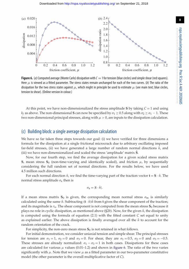
Figure 6. (a) Computed average (Monte Carlo) dissipation with C = 1 for tension (blue circles) and simple shear (red squares).Here μ is viewed as a fitted parameter. The stress states remain unchanged for each of the two curves. (b) The ratio of thedissipation for the two stress states against μ, which might in principle be used to estimate μ (see main text; blue circles,tension to shear). (Online version in colour.)

At this point, we have non-dimensionalized the stress amplitude S by taking C = 1 and usingkf as above. The non-dimensional S can now be specified by σ1 ≥ 0.5 along with σ2 ≥ σ1 − 1. Thesetwo non-dimensional principal stresses, along with μ > 0, are inputs to the dissipation calculation.

(c) Building block: a single average dissipation calculationWe have so far taken three steps towards our goal: (i) we have verified for three dimensions aformula for the dissipation at a single frictional microcrack due to arbitrary oscillating imposedfar-field stresses, (ii) we have generated a large number of random normal directions n, and(iii) we have non-dimensionalized and scaled the stress ‘amplitude’ matrix S.

Now, for our fourth step, we find the average dissipation for a given scaled stress matrixS, mean stress S0 (non-time-varying and identically scaled), and friction μ, by sequentiallyconsidering the full random set of normal directions. For the results below, we have used4.5 million such directions.

For each normal direction n, we find the time-varying part of the traction vector t = S · n. Thenormal stress amplitude σa then is

σa = |t · n|.

If a mean stress matrix S0 is given, the corresponding mean normal stress σm is similarlycalculated using the same n. Subtracting (t · n)n from t gives the shear component of the traction;and its magnitude is τa. The shear component is not computed from the mean stress S0 because itplays no role in cyclic dissipation, as mentioned above (§2b). Now, for the given n, the dissipationis computed using the formula of equation (2.1) with the fitted constant C set equal to unityas explained earlier. The above dissipation is finally averaged over all the n to account for therandom orientation of the crack.

For simplicity, the non-zero mean stress S0 is not retained in what follows.For initial demonstration, we consider uniaxial tension and simple shear. The principal stresses

for tension are σ1 = 1, σ2 = 0 and σ3 = 0. For shear, they are σ1 = 0.5, σ2 = 0 and σ3 = −0.5.These stresses are already normalized: σ1 − σ3 = 1 in both cases. Dissipations for these casesare calculated for various μ values (0.01–1.2) and shown in figure 6. The ratio of the two variessignificantly with μ. Note that we view μ as a fitted parameter in our two-parameter constitutivemodel (the other parameter is the overall multiplicative factor of C).

9

rspa.royalsocietypublishing.orgProcRSocA469:20120685

..................................................

on September 21, 2018http://rspa.royalsocietypublishing.org/Downloaded from

As an example of how μ might be fitted consider Robertson & Yorgiadis [20], who sought thesame specific dissipation per cycle in two different loading conditions.3 For such equal dissipationto occur under both pure (simple) shear and pure extension, the ratio of the shear stress amplitudeduring torsional vibration to the normal stress amplitude during longitudinal vibration wasfound to be between 0.48 and 0.60 (for several materials). This statement of equivalence translates,for our model, into roughly 0.6 < μ < 1.1 by the following reasoning. Fix the longitudinal stressstate at σ1 = 1, σ2 = 0 and σ3 = 0, as above. Let the shearing stress state be σ1 = 0.5, σ2 = 0 andσ3 = −0.5 but only after normalization by some factor k; in other words, the applied shear stresswould be of amplitude k/2. Since the shear stress amplitudes found by Robertson & Yorgiadis [20]are between 0.48 and 0.6, k lies between 0.96 and 1.2. If k = 0.96, the dissipation in shear will be0.962 ≈ 0.92 times the value in figure 6a. Alternatively, the ratio plotted in figure 6b, upon divisionby 0.92, should give 1, implying μ ≈ 1.1. Similarly, if k = 1.2, we find μ ≈ 0.6.

4. Fitted formulaSo far, the dissipation has been computed as a function of S, possibly a non-zero S0, and μ, usinga time-consuming Monte Carlo simulation.

However, we eventually want to compute the modal damping of a given object of arbitraryshape. For each mode, the stress state varies spatially. We cannot do Monte Carlo simulations forevery point on the body. So our fifth step is to summarize the dissipation values obtained fromMonte Carlo simulations, for the special case of S0 = 0, using a quick multivariate polynomial fit.

(a) A comment on prior effortsTo motivate our multivariate fitted formula, we first note some prior attempts at ad hoc modellingof material dissipation under multiaxial stress states. Recall equation (1.1), wherein a suitableequivalent stress amplitude needs to be defined. Damping under biaxial stresses has been studiedby several authors, including Robertson & Yorgiadis [20], Whittier [21], Torvik et al. [22] andMentel & Chi [23]. A review of these articles is given in the electronic supplementary material.All these authors considered at least one ad hoc definition equivalent to equation (1.2), possiblyrearranged or differently normalized. But if equation (1.2) had general validity it would applyto our dissipation results as well, since these are derived from legitimate (though approximated)physics. To check the same, we can rewrite equation (1.2) as

D ≈ λ1{(σ1 − σ2)2 + (σ2 − σ3)

2 + (σ3 − σ1)2} + λ2(σ1 + σ2 + σ3)

2, (4.1)

where the λ’s are fitted coefficients, and the assumed roles of the distortional and dilatationalstrain energies are clearly visible. In checking equation (4.1) against our dissipation results, wenote that different μ represent different material behaviours, and so we should work with one μ

at a time. Figure 7a,b shows least-squares fitted comparisons for two μ values. The poor matchindicates both the inapplicability of equation (4.1) in general cases and motivates our multivariatepolynomial fit below.

(b) Inputs to the fitted multivariate polynomial formulaThe scaled stress S and μ are inputs for our dissipation calculation. We will later divide thecomputed dissipation by k2

f (see equations (3.1) and (3.2)) to obtain the dissipation for the actual

stress S. We now introduce two new scaled variables.

3A brief review of other multiaxial dissipation experiments is given in the electronic supplementary material.

10

rspa.royalsocietypublishing.orgProcRSocA469:20120685

..................................................

on September 21, 2018http://rspa.royalsocietypublishing.org/Downloaded from

0 0.005 0.010 0.015–2

0

2

4

6

8

10

12

14

16fi

tted

diss

ipat

ion

(× 1

0–3)

actual dissipation actual dissipation

0 0.004

(a) (b)

0.008 0.012 0.016–5

0

5

10

15

20

Figure 7. Comparison of equation (4.1) against our dissipation model for twoμ ((a)μ = 0.5; (b)μ = 0.9) values (differentleast-squares fits used in each subplot, for λ1 and λ2). The plotted straight lines are at 45◦, for reference. These plots may becompared against figure 9b. (Online version in colour.)

diss

ipat

ion

0.51.0

1.52.0

2.5

0

0.5

1.00

0.005

0.010

0.015

0.020

0.025

(a) (b)

0.51.0

1.5

0

0.5

1.00

0.005

0.010

0.015

0.020

diss

ipat

ion

s1

cs1

c

Figure 8. Dissipation surface plots for twoμ ((a)μ = 0.3; (b)μ = 0.6) values. (Online version in colour.)

First, define χ = σ1 − σ2. The inequality σ1 − 1 ≤ σ2 ≤ σ1 becomes 0 ≤ χ ≤ 1. Figure 5b showsthe non-zero-dissipation range of σ1 as 0.5 ≤ σ1 ≤ σ1cr, where

σ1cr = 12

+√

1 + μ2

2μ. (4.2)

For σ1 ≥ 0.5 and 0 ≤ χ ≤ 1, with μ as a parameter, we now generate surface plots of thedissipation as computed from Monte Carlo simulations. We compute 11 such surface plots, forequally spaced μ values from 0.2 to 1.2. Two representative plots are shown in figure 8; anothernine are given in the electronic supplementary material. The figure confirms that the dissipationdoes become zero for each μ when σ1 crosses σ1cr (equation (4.2)). We now introduce a final scaledvariable

s = 1 − (σ1 − 0.5)

(σ1cr − 0.5), (4.3)

such that there is non-zero dissipation only for s > 0. We will now seek a single fitted formula forall these dissipation surfaces, given s, χ and μ.

11

rspa.royalsocietypublishing.orgProcRSocA469:20120685

..................................................

on September 21, 2018http://rspa.royalsocietypublishing.org/Downloaded from

(c) Multivariate polynomial fitRecall equation (2.1). Now setting C = 1 (different C will be incorporated later), and for β = 0 (zeromean stress), we write

Df = average of{

[ζ > μ] × σ 2a μζ

ζ − μ

ζ + μ

}, (4.4)

where the average is over all possible orientations of the crack face. We propose, for simplicity, apolynomial form for the fit:

Df =∑

m0,m1,m2

Bm0m1m2 sm0χm1μm2 , 1 ≤ m0 ≤ 5, 0 ≤ m1 ≤ 4, 0 ≤ m2 ≤ 3, (4.5)

where the Bm0m1m2 ’s collectively denote 100 fitted coefficients. Our numerical fit will be muchfaster than Monte Carlo simulation, and given below in an easily portable form. In particular, Dfwill be written as a product of three matrices, ABM, and the constitutive relation for dampingwill be

D = C × [s > 0] × ABM. (4.6)

Here D (as before) is the dissipation per unit volume and per stress cycle due to scaled stress S,C is a fitted scalar coefficient, [s > 0] is a logical variable that ensures zero dissipation for s ≤ 0(see equation (4.3)), M is a column vector containing powers of χ as described below, A is a rowvector containing products of powers of s and μ as described below and the matrix B containsfitted numerical coefficients.

We write M and A as follows:

M = [1 χ χ2 χ3 χ4]T and A = [A0 A1 A2 A3], (4.7)

with A0 = [s s2 s3 s4 s5] and Am = μmA0.The fitted 20 × 5 matrix B, determined from a least-squares calculation, is given in appendix A.

In the fit, the maximum absolute error as a percentage of the maximum for each corresponding μ

is within 5.2 per cent, with typical errors being substantially smaller.Figure 9a shows the quality of the fit using two surface plots for μ = 0.4. One surface is from

Monte Carlo simulation (accurate) and the other is from the fitted polynomial. The match isgood. Another comparison is shown in figure 9b, where all the data points used in the fit areplotted, fitted value against original Monte Carlo value, along with a 45◦ line. Within this plot arerepresented 11 equally spaced μ values from 0.2 to 1.2. The match is reasonably good, and can beimproved if desired by using higher order polynomials or other fitting methods. But dissipation,similar to other non-ideal material behaviours involving friction, fracture and plasticity, is difficultto model accurately in any case; so we arbitrarily chose to limit the number of fitting coefficientsto 100, arranged in a matrix that is easy to cut and paste.

An illustration of our dissipation calculation is now given for completeness. Let the state ofstress be

S =

⎡⎢⎣1 2 3

2 5 43 4 6

⎤⎥⎦ ,

an arbitrary choice. The principal stresses are σ1 = 10.833, σ2 = 1.577, σ3 = −0.410. The scalingfactor kf = 0.089 and the normalized eigenvalues work out to σ1 = 0.964, σ2 = 0.140, σ3 = −0.036,giving χ = 0.824. We take μ = 0.5. Then σ1cr = 1.618, giving s = 0.585. Now using equation (4.6)with C = 1, we find D = 0.014. Finally, the dissipation is D/(kf )

2 = 1.818 in appropriate units.Two further aspects of the fit are mentioned here.

12

rspa.royalsocietypublishing.orgProcRSocA469:20120685

..................................................

on September 21, 2018http://rspa.royalsocietypublishing.org/Downloaded from

s1

c

diss

ipat

ion

(a) (b)

dissipation (Monte Carlo method)

diss

ipat

ion

(fitt

ed f

orm

ula)

0.51.0

1.52.0

0

0.5

1.00

0.005

0.010

0.015

0.020

0 0.005 0.010 0.015 0.020

0.005

0.010

0.015

0.020

Figure 9. Dissipation comparisonwith C = 1: (a) surface plots forμ = 0.4, (b) for allμ values (a 45◦ line is also shown in thisplot). (Online version in colour.)

First, the polynomial fit occasionally predicts some small negative values, as suggested by thebottom left portion of figure 9b. We simply replace those negative predictions with zero, withnegligible consequence because such values are both infrequently encountered and small.

Secondly, the dissipation computation using our fitted formula is very fast compared withthe Monte Carlo Method. A total of 10 000 evaluations of the formula took about 0.2 s on anunremarkable desktop computer, where a single Monte Carlo evaluation with 4.5 million points(found separately to be large enough for the accuracy needed) took about 3 min.

5. Finite-element computation of modal dampingWe have now completed all the steps needed to consider the effective modal damping of anygiven mode of an arbitrarily shaped object. We will illustrate our calculations using the solidbody shown in figure 1a.

For completeness, we have included a brief introduction to relevant aspects of vibration theoryin the electronic supplementary material. The key ideas are summarized as follows. The dampingmechanism we have considered is nonlinear, but the damping is assumed to be small. Forsmall damping, the damping plays no significant role except near resonance. Near each distinctresonant frequency (or natural frequency) of an arbitrary body, an effective damping ratio forthe corresponding mode can be defined. This section is concerned with the computation of sucheffective modal damping values.

(a) Effective damping ratio (ζeff)

We begin with an elementary formula. A lightly damped harmonic oscillator of the form

x + 2ζωnx + ω2nx = 0, (5.1)

has damping ratio ζ which, to first order, is equivalent to

ζeff = 14π

×(

−�E

E

), (5.2)

where −�E is the energy dissipated per oscillation, E is the total energy of the system averagedover one cycle and the bar is to distinguish the energy from Young’s modulus which will be

13

rspa.royalsocietypublishing.orgProcRSocA469:20120685

..................................................

on September 21, 2018http://rspa.royalsocietypublishing.org/Downloaded from

0 50 100 150 200–1.0

–0.8

–0.6

–0.4

–0.2

0

0.2

0.4

0.6

0.8

1.0

time, t

x(t)

and

its

ampl

itude

env

elop

e

Figure 10. Numerical solution of equation (5.3) using MATLAB’s ‘ode15 s’. The initial condition was changed from x(0) = 0 tox(0) = 10−10 to avoid the immediate discontinuity at zero. The amplitude envelope approximation of e−ct/π matches near-perfectly. (Online version in colour.)

discussed later. Equation (5.2) works only for lightly damped systems because −�E is computedover a cycle by assuming a harmonic solution. However, it is general: it does not need a linearviscous model. The general unforced solution is then approximated as

x ≈ e−ζωntA cos(√

1 − ζ 2 ωnt + φ).

For small ζ , we may often just write

x ≈ e−ζωntA cos(ωnt + φ).

For a simple analytical example, consider

x + c|x|sign(x) + x = 0. (5.3)

Assume first an approximate solution (neglecting the damping over one cycle) of

x ≈ A sin t and E = A2

2,

from the maximum potential or kinetic energy. The energy dissipation per cycle is, by thisapproximation,

− �E =∫ 2π

0c|x|sign(x)x dt = cA2

∫ 2π

0| sin(t) cos(t)| dt = 2 cA2, (5.4)

whence by equation (5.2) we have

ζeff = cπ

.

A numerical solution of the nonlinear equation (5.3) with c = 0.1 and initial conditions x(0) = 1and x(0) = 0 is shown in figure 10. A plot of e−ct/π is also given for comparison and is seen tomatch the oscillation envelope very well.

The above example shows the utility of equation (5.2), which we will use below. The energydissipation calculation below will use our fit of equation (4.6), suitably integrated over the entirevibrating object.

14

rspa.royalsocietypublishing.orgProcRSocA469:20120685

..................................................

on September 21, 2018http://rspa.royalsocietypublishing.org/Downloaded from

1

MN

MX

XY

Z

0.664E-030.008652

0.0166390.024626

0.0326130.0406

0.0485870.056575

0.0645620.072549

NOV 9 201213:49:15

NODAL SOLUTION

STEP = 1SUB = 8FREQ = 123.029USUM (AVG)RSYS = SOLUDMX = 0.072549SMN = 0.664E-03SMX = 0.072549

1

MN

MX

XY

Z

0.287E-030.007036

0.0137850.020535

0.0272840.034033

0.0407820.047531

0.0542810.06103

NOV 9 201213:49:34

NODAL SOLUTION

STEP = 1SUB = 9FREQ = 195.608USUM (AVG)RSYS = SOLUDMX = 0.06103SMN = 0.287E-03SMX = 0.06103

(a) (b)

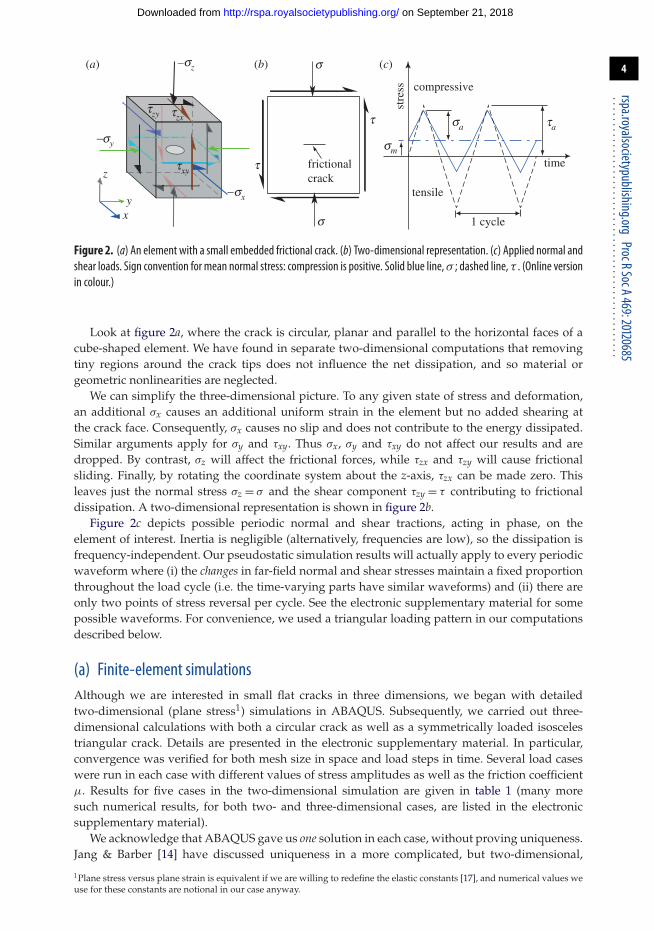
Figure 11. Vibration modes of the solid body: (a) second mode, (b) third mode. The first mode was shown in figure 1b. (Onlineversion in colour.)

(b) Finite-element prediction of effective damping ratioOur FE computation of mode shapes and modal damping proceeds as follows. We have usedthe FE package ANSYS for modal analysis and related computations in this paper. Elementwiseintegrals below will use Gaussian quadrature [24].

The vibrating object of interest is first meshed using 10 noded tetrahedral elements (SOLID187)using automatic meshing within ANSYS. Modal analysis in ANSYS yields natural frequenciesand mass-normalized mode shapes. Nodal displacements for each mode of interest are extractedusing a small external program.

Using the element shape functions and the nodal displacements, the displacement field iscomputed and then differentiated to obtain strains, and thence stresses, at four Gauss pointsper element. At each Gauss point, the stress is used in conjunction with equation (4.6) tocompute the dissipation per unit volume and per cycle. The dissipation in the element is thenobtained by the usual weighted sum of its values at the Gauss points; and the same is addedup for all elements to obtain the total energy dissipated per cycle in the vibrating object. Thisdissipation is −�E.

E is simply ω2/2 because the mode shape is mass normalized.Now the effective damping ratio is obtained using equation (5.2). Some further details are

provided in the electronic supplementary material.

(c) Results for an arbitrary solid objectWe finally consider the solid object shown in figure 1a. It is not special, and merely representsan object that is difficult or impractical to treat analytically. The object is an unconstrained thickcircular plate of radius 1 m and thickness 0.1 m, with a square hole. The edges of the hole are0.4 m, and its centre is 0.5 m from the centre of the circle. Young’s modulus (E), Poisson’s ratio (ν)and density (ρ) of the material are arbitrarily taken as 100 GPa, 0.28 and 4000 kg m−3, respectively.

A total of 32 418 elements were used for meshing the object. The effective damping wascomputed for the first three vibration modes. The first mode was shown in figure 1b. The secondand third modes are shown in figure 11.

Noting that C has units of Pa−1, we have arbitrarily chosen C = 2π/E, where the dependenceon E is motivated by the units and the 2π ensures that, for axial vibrations of a uniform rod, theeffective damping is exactly equal to Df in equation (4.5). In real applications, where C would befitted from test data, the 2π would be replaced with a fitted constant.

15

rspa.royalsocietypublishing.orgProcRSocA469:20120685

..................................................

on September 21, 2018http://rspa.royalsocietypublishing.org/Downloaded from

0.2 0.4 0.6 0.8 1.0 1.20.002

0.004

0.006

0.008

0.010

0.012

0.014

0.016

0.018

friction coefficient, m

effe

ctiv

e da

mpi

ng, (

2p/E

)zef

f

friction coefficient, m

(a) (b)

z eff,

3rd/

z eff,

1st

0.2 0.4 0.6 0.8 1.0 1.2

0.4

0.5

0.6

0.7

0.8

0.9

1.0

1.1

0.3

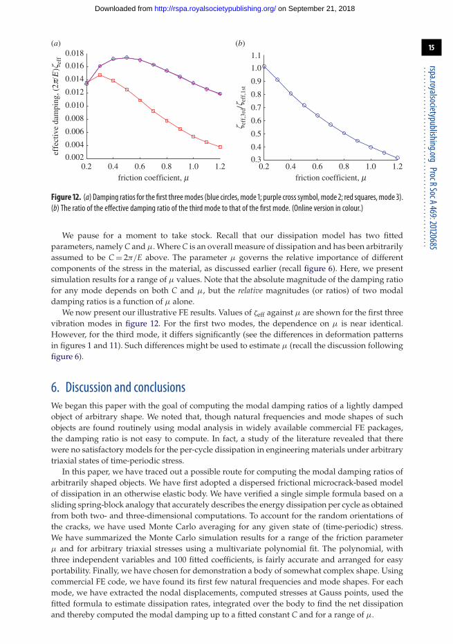
Figure 12. (a) Damping ratios for the first threemodes (blue circles,mode 1; purple cross symbol,mode 2; red squares,mode 3).(b) The ratio of the effective damping ratio of the third mode to that of the first mode. (Online version in colour.)

We pause for a moment to take stock. Recall that our dissipation model has two fittedparameters, namely C and μ. Where C is an overall measure of dissipation and has been arbitrarilyassumed to be C = 2π/E above. The parameter μ governs the relative importance of differentcomponents of the stress in the material, as discussed earlier (recall figure 6). Here, we presentsimulation results for a range of μ values. Note that the absolute magnitude of the damping ratiofor any mode depends on both C and μ, but the relative magnitudes (or ratios) of two modaldamping ratios is a function of μ alone.

We now present our illustrative FE results. Values of ζeff against μ are shown for the first threevibration modes in figure 12. For the first two modes, the dependence on μ is near identical.However, for the third mode, it differs significantly (see the differences in deformation patternsin figures 1 and 11). Such differences might be used to estimate μ (recall the discussion followingfigure 6).

6. Discussion and conclusionsWe began this paper with the goal of computing the modal damping ratios of a lightly dampedobject of arbitrary shape. We noted that, though natural frequencies and mode shapes of suchobjects are found routinely using modal analysis in widely available commercial FE packages,the damping ratio is not easy to compute. In fact, a study of the literature revealed that therewere no satisfactory models for the per-cycle dissipation in engineering materials under arbitrarytriaxial states of time-periodic stress.

In this paper, we have traced out a possible route for computing the modal damping ratios ofarbitrarily shaped objects. We have first adopted a dispersed frictional microcrack-based modelof dissipation in an otherwise elastic body. We have verified a single simple formula based on asliding spring-block analogy that accurately describes the energy dissipation per cycle as obtainedfrom both two- and three-dimensional computations. To account for the random orientations ofthe cracks, we have used Monte Carlo averaging for any given state of (time-periodic) stress.We have summarized the Monte Carlo simulation results for a range of the friction parameterμ and for arbitrary triaxial stresses using a multivariate polynomial fit. The polynomial, withthree independent variables and 100 fitted coefficients, is fairly accurate and arranged for easyportability. Finally, we have chosen for demonstration a body of somewhat complex shape. Usingcommercial FE code, we have found its first few natural frequencies and mode shapes. For eachmode, we have extracted the nodal displacements, computed stresses at Gauss points, used thefitted formula to estimate dissipation rates, integrated over the body to find the net dissipationand thereby computed the modal damping up to a fitted constant C and for a range of μ.

16

rspa.royalsocietypublishing.orgProcRSocA469:20120685

..................................................

on September 21, 2018http://rspa.royalsocietypublishing.org/Downloaded from

We anticipate that this line of work may have useful applications and extensions in futurework. Clearly, such modelling provides a route to optimizing engineering component designs fordamping. Additionally, such work may lead to new academic research towards incorporatingresidual stresses, other dissipation mechanisms, anisotropy in material properties or flawdistributions, interactions between flaws, etc. Finally, we hope that such constitutive relationsmight eventually be built into commercial FE codes, so that modal damping values could becomputed and compared routinely along with natural frequencies and mode shapes.

We thank Arghya Deb, Vikranth Racherla and A. K. Mallik for discussions, and the Department of Science andTechnology, Government of India, for financial support. Anonymous reviewers raised questions that helpedimprove the paper.

Appendix A. Matrix B for the constitutive modelFor equation (4.6), the fitted matrix B was found to be

B =

⎡⎢⎢⎢⎢⎢⎢⎢⎢⎢⎢⎢⎢⎢⎢⎢⎢⎢⎢⎢⎢⎢⎢⎢⎢⎢⎢⎢⎢⎢⎢⎢⎢⎢⎢⎢⎢⎢⎢⎣

0.0502 −0.2919 1.4014 −2.2672 1.2207−0.2404 1.1032 −8.5528 15.6248 −8.84440.9590 −1.9703 19.1510 −37.1280 22.1110

−1.3023 1.7092 −18.3802 37.1835 −23.22540.5354 −0.5540 6.3899 −13.4358 8.7562

−0.1639 0.2904 −2.4921 5.2895 −3.47131.4849 −1.5920 22.4593 −53.7902 37.0354

−4.4902 5.6752 −70.7569 170.3431 −117.58535.0411 −8.3716 88.1836 −208.9717 143.4247

−1.8201 3.9436 −37.2935 87.0923 −59.41260.2007 −0.3217 3.4993 −8.2660 5.6588

−1.8590 3.0802 −34.4736 84.1598 −58.34005.0382 −11.5023 111.2467 −266.1229 182.3608

−5.0664 16.2774 −139.9197 326.2059 −220.42251.6216 −7.4579 59.4630 −135.8272 90.6983

−0.0755 0.1573 −1.6178 3.8573 −2.63400.6723 −1.6798 15.9470 −38.2460 26.1804

−1.6712 5.9580 −50.6344 118.6870 −80.14941.5056 −8.0587 62.8622 −143.7174 95.6099

−0.4069 3.5941 −26.4779 59.3444 −38.9797

⎤⎥⎥⎥⎥⎥⎥⎥⎥⎥⎥⎥⎥⎥⎥⎥⎥⎥⎥⎥⎥⎥⎥⎥⎥⎥⎥⎥⎥⎥⎥⎥⎥⎥⎥⎥⎥⎥⎥⎦

.

References1. Lord Kelvin (W. Thomson). 1865 On the elasticity and viscosity of metals. Proc. R. Soc. Lond.

14, 289–297. (doi:10.1098/rspl.1865.0052)2. Rowett FE. 1914 Elastic hysteresis in steel. Proc. R. Soc. Lond. A 89, 528–543. (doi:10.1098/

rspa.1914.0021)3. Kimball AL, Lovell DE. 1927 Internal friction in solids. Phys. Rev. 30, 948–959. (doi:10.1103/

PhysRev.30.948)4. Lazan BJ. 1968 Damping of materials and members in structural mechanics. New York, NY:

Pergamon Press.5. Granato A, Lücke K. 1956 Theory of mechanical damping due to dislocations. J. Appl. Phys.

27, 583–593. (doi:10.1063/1.1722436)6. Dawson TH. 1978 Continuum description of hysteresis damping of vibration. Int. J. Solids

Struct. 14, 457–464. (doi:10.1016/0020-7683(78)90010-0)7. Hooker RJ. 1969 Equivalent stresses for representing damping in combined stress. J. Sound

Vib. 10, 62–70. (doi:10.1016/0022-460X(69)90129-1)8. Kachanov M. 1987 Elastic solids with many cracks: a simple method of analysis. Int. J. Solids

Struct. 23, 23–43. (doi:10.1016/0020-7683(87)90030-8)

17

rspa.royalsocietypublishing.orgProcRSocA469:20120685

..................................................

on September 21, 2018http://rspa.royalsocietypublishing.org/Downloaded from

9. Aleshin V, Abeele KVD. 2007 Friction in unconforming grain contacts as a mechanismfor tensorial stress–strain hysteresis. J. Mech. Phys. Solids 55, 765–787. (doi:10.1016/j.jmps.2006.10.001)

10. Deshpande VS, Evans AG. 2008 Inelastic deformation and energy dissipation in ceramics: amechanism-based constitutive model. J. Mech. Phys. Solids 56, 3077–3100. (doi:10.1016/j.jmps.2008.05.002)

11. Abu Al-Rub RK, Palazotto AN. 2010 Micromechanical theoretical and computationalmodeling of energy dissipation due to nonlinear vibration of hard ceramic coatings withmicrostructural recursive faults. Int. J. Solids Struct. 47, 2131–2142. (doi:10.1016/j.ijsolstr.2010.04.016)

12. Jang YH, Barber JR. 2011 Frictional energy dissipation in materials containing cracks. J. Mech.Phys. Solids 59, 583–594. (doi:10.1016/j.jmps.2010.12.010)

13. Barber JR, Davies M, Hills DA. 2011 Frictional elastic contact with periodic loading. Int. J.Solids Struct. 48, 2041–2047. (doi:10.1016/j.ijsolstr.2011.03.008)

14. Jang YH, Barber JR. 2011 Effect of phase on the frictional dissipation in systems subjectedto harmonically varying loads. Eur. J. Mech. A/Solids 30, 269–274. (doi:10.1016/j.euromechsol.2011.01.008)

15. Barber JR. 2011 Frictional systems subjected to oscillating loads. Ann. Solid Struct. Mech. 2,45–55. (doi:10.1007/s12356-011-0017-5)

16. Putignano C, Ciavarella M, Barber JR. 2011 Frictional energy dissipation in contact ofnominally flat rough surfaces under harmonically varying loads. J. Mech. Phys. Solids 59,2442–2454. (doi:10.1016/j.jmps.2011.09.005)

17. Timoshenko SP, Goodier JN. 1951 Theory of elasticity. New York, NY: McGraw-Hill BookCompany.

18. Barquins M. 1985 Sliding friction of rubber and Schallamach waves: a review. Mater. Sci. Eng.73, 45–63. (doi:10.1016/0025-5416(85)90295-2)

19. Malvern LE. 1969 Introduction to the mechanics of a continuous medium. Englewood Cliffs, NJ:Prentice-Hall.

20. Robertson JM, Yorgiadis AJ. 1946 Internal friction in engineering materials. Trans. Am. Soc.Mech. Eng. 68, A173–A182.

21. Whittier JS. 1962 Hysteretic damping of structural materials under biaxial dynamic stresses.Exp. Mech. 2, 321–328. (doi:10.1007/BF02326136)

22. Torvik PJ, Chi SH, Lazan BJ. 1963 Damping of materials under biaxial stress. Wright–PattersonAir Force Base Technical Documentary Report, no. ASD-TDR-62-1030.

23. Mentel TJ, Chi SH. 1964 Experimental study of dilatational- versus distortional-strainingaction in material-damping production. J. Acoust. Soc. Am. 36, 357–365. (doi:10.1121/1.1918961)

24. Bathe KJ. 1996 Finite element procedures. Englewood Cliffs, NJ: Prentice-Hall.