Analytical stability conditions for elastic composite...

Proc. R. Soc. A (2012) 468, 2230–2254doi:10.1098/rspa.2011.0546

Published online 14 March 2012

Analytical stability conditions for elasticcomposite materials with anon-positive-definite phase

BY D. M. KOCHMANN1,* AND W. J. DRUGAN2

1Graduate Aerospace Laboratories, California Institute of Technology,Pasadena, CA 91125, USA

2Department of Engineering Physics, University of Wisconsin–Madison,Madison, WI 53706, USA

Elastic multi-phase materials with a phase having appropriately tuned non-positive-definite elastic moduli have been shown theoretically to permit extreme increasesin multiple desirable material properties. Stability analyses of such composites wereonly recently initiated. Here, we provide a thorough stability analysis for generalcomposites when one phase violates positive-definiteness. We first investigate the dynamicdeformation modes leading to instability in the fundamental two-phase solids of acoated cylinder (two dimensions) and a coated sphere (three dimensions), from which wederive closed-form analytical sufficient stability conditions for the full range of coatingthicknesses. Next, we apply the energy method to derive a general correlation betweencomposite stability limit and composite bulk modulus that enables determination ofclosed-form analytical sufficient stability conditions for arbitrary multi-phase materialsby employing effective modulus formulas coupled with a numerical finite-element stabilityanalysis. We demonstrate and confirm this new approach by applying it to (i) thetwo basic two-phase solids already analysed dynamically; and (ii) a more geometricallycomplex matrix/distributed-inclusions composite. The specific new analytical stabilityresults, and new methods presented, provide a basis for creation of novel, stablecomposite materials.

Keywords: stability; elasticity; composite material; negative stiffness

1. Introduction

Materials with counterintuitive physical properties have recently attractedincreasing attention, resulting in novel solids having negative Poisson’s ratio(Lakes 1987), negative thermal expansion (Mary et al. 1996), negative refractiveindex (Shelby et al. 2001), negative effective mass density (Liu et al. 2005) andnegative elastic stiffness in a constrained composite phase (Jaglinski et al. 2007).

Composite materials have long offered a convenient approach to creatematerials with enhanced performance by combining several materials onvarious length scales. The overall properties of a composite result from*Author for correspondence ([email protected]).

Received 9 September 2011Accepted 15 February 2012 This journal is © 2012 The Royal Society2230

on July 29, 2018http://rspa.royalsocietypublishing.org/Downloaded from

mailto:[email protected]

http://rspa.royalsocietypublishing.org/

Stability of elastic composites 2231

the individual specifics of the constituent materials (often called phases),their shape, geometrical arrangement and bonding (Milton 2001). Whileclassical composite materials theory contemplated combining materials allhaving ‘positive’ properties, and the bounds thereby obtained provided perhapsunsurprising limits on the achievable composite response, the possibility ofcombining materials having positive and negative properties offers the tantalizingprospect of dramatically improved composite behaviour that can far exceedthe classical bounds by relaxing an assumption on which all these boundsrely. Indeed, classical composite materials formulas (as well as exact elasticitysolutions) for the overall response of a composite with an appropriately tunednegative-property phase predict a response far exceeding the classical bounds,which were long regarded as the absolute limits of the achievable. A primeexample is a linear elastic solid, whose elastic moduli are constrained by upperand lower bounds in terms of, for conventional materials, the constituents’moduli and volume fractions (Voigt 1889; Reuss 1929; Paul 1960; Hill 1963;Hashin & Shtrikman 1963). When incorporating one phase having appropriatelytuned non-positive-definite elastic moduli (i.e. negative stiffness), however, theclassical bounds can be dramatically surpassed (Lakes & Drugan 2002). (Modelsincorporating viscoelasticity and finite deformation confirm the bound-exceedingperformance.) Multiple additional composite properties can achieve extremevalues via a tuned negative-stiffness phase, e.g. damping capacity, thermalexpansion, piezoelectricity and pyroelectricity (Lakes 2001; Wang & Lakes 2001,2004, 2006).

Violation of positive-definiteness of the elastic moduli raises stability issues.It is well known that a homogeneous, unconstrained, linear elastic bodymust have positive-definite elastic moduli to be stable overall (Kelvin 1888).However, Drugan (2007) and Kochmann & Drugan (2009) recently provedthat the geometrical constraint imposed by an encapsulating positive-definitephase in a composite can provide sufficient stabilization to permit violation ofpositive-definiteness in the composite’s encapsulated phase, while the compositeremains stable overall. The derivation of the stability conditions for compositesis in general quite complex, requiring numerical evaluation except for veryspecial cases.

Thus, the main goal of this paper is to introduce methods for deriving closed-form analytical sufficient conditions for the stability of two-phase solids andgeneral composite materials, and to employ these to derive new specific resultsfor several important basic composite geometries.

2. Incremental stability conditions for elastic solids

The state of strain in a body experiencing infinitesimal displacement gradientsis characterized by the symmetric infinitesimal strain tensor 3ij = 1

2(ui,j + uj ,i),where u is the displacement vector field and a comma in a subscript denotesdifferentiation with respect to the ensuing coordinate(s). For a linear elastic solid,the symmetric stress tensor s is related to the strain tensor via Hooke’s law,sij = Cijkl3kl , C being the fourth-order tensor of elastic moduli. If the solid is alsoisotropic, the modulus tensor contains only two independent scalar moduli, e.g.the shear and bulk moduli, m and k, respectively; or Young’s modulus E and

Proc. R. Soc. A (2012)



2232 D. M. Kochmann and W. J. Drugan

Poisson’s ratio n; or the Lamé moduli l and m. For the last case, Cijkl = l dijdkl +m(dikdjl + dildjk) so that sij = 2m3ij + l3kkdij , where dij is the Kronecker delta. Thestrain energy density is J(3) = 1

23ijsij(3) = 123ijCijkl3kl .

The stability of an elastic body can be investigated by several different methodsyielding different conditions in general. First, it is essential to differentiatebetween material and structural conditions of stability of a macroscopic solid.The conditions of material stability (Mandel 1966) are local in nature and derivedfrom the governing (pointwise) differential equations of the elastic medium byrequiring that acceleration waves can propagate at finite speeds. Therefore, thematerial conditions of stability ensure real-valuedness of the speed of travellingwaves, which requires strong ellipticity of the stiffness tensor C (Kelvin 1888)and positive-definiteness of the acoustic tensor T(n) with components Tij(n) =Ckijlnk nl in every direction n (Mandel 1962). They also imply rank-one convexityof the strain energy density. For an isotropic, linear elastic material, the conditionsof material stability reduce to m > 0 and l + 2m > 0.

The conditions of structural stability, in contrast, are non-local and ensurestability of the overall body. Satisfying these guarantees that an arbitraryinfinitesimal perturbation of the displacement field from an equilibrium stateremains infinitesimal for all time. (It is important to note that this only appliesto infinitesimal perturbations; therefore, one may speak of incremental stabilityin this context. For a sufficiently large imposed perturbation, the system maybecome unstable and deform into the next stable state. However, as we focuson linear elasticity, the condition of incremental stability is sufficient for ourpurposes.) The conditions of structural stability are derived from either energeticconsiderations, enforcing uniqueness of solutions or quasi-convexity of the energy(Kirchhoff 1859; Morrey 1952; Pearson 1956; Hill 1957), or from a dynamicapproach that seeks to analyse the eigenmodes of a free vibration with respectto stability in the sense of Lyapunov (1966). The energy method yields theconditions of so-called static stability, whereas the dynamic approach determineskinematic stability (Ziegler 1953). While both methods provide identical resultsfor conservative systems (Koiter 1965) (such as the linear elastic compositesstudied in the sequel), they differ for non-conservative systems (e.g. if circulatoryor gyroscopic forces are present; cf. Kochmann & Drugan 2011), where onlythe dynamic approach yields the correct structural stability conditions (Ziegler1953). For an externally unconstrained homogeneous solid, the conditions ofstructural stability require positive-definiteness of the fourth-order stiffnesstensor, which, for an isotropic, linear elastic medium reduces to m > 0 andk > 0. Owing to the different forms of the effective bulk modulus k, theseconditions are interpreted differently in terms of the Lamé moduli in two andthree dimensions: m > 0 and l + 2

3m > 0 must hold in three dimensions, whilem > 0 and l + m > 0 are the corresponding conditions in two dimensions (i.e.plane strain).

For a macroscopic solid without microstructure, the local conditions of materialstability are necessary, and the non-local conditions of structural stability aresufficient for overall stability. The situation becomes more complex when studyingstability in microstructured solids with randomized or periodic microstructurewhere cooperative phenomena may arise. Here, the two conditions guaranteeperiodic (local or short wavelength) stability and long-range (or long wavelength)stability, respectively, and both conditions must be checked independently to





ensure overall stability. In particular, in a composite with a distinct separation ofmacro- and micro-length scales, structural stability on the microscale correspondsto material stability on the macroscale.

Sufficient stability conditions for complex composite geometries are generallydifficult to determine analytically, necessitating numerical techniques. Kochmann(in press) showed how sufficient (static) conditions of stability for compositeswith negative-stiffness phases can be obtained in a straightforward mannerfrom a modal decomposition and eigenvalue analysis based on a finite-elementformulation. As shown there, it is a simple exercise to verify that the sufficientcondition of stability for an elastic composite (i.e. the condition of structuralstability) translates into the requirement of positive-definiteness of the overallstiffness matrix K of the finite-element model. For the separable displacementfield of the form u(x , t) = v(x) eiu t , this can be verified by computing Rayleigh’squotient, which provides an upper bound on the (squared) lowest eigenfrequencyu0 of the body:

u20 ≤ vTKv

vTMv, (2.1)

where M is the mass matrix and v the vector of all nodal displacements.Equality holds if and only if v is the eigenvector corresponding to the lowestmode; otherwise, the quotient provides an upper bound for arbitrary v ∈ R

d ,v �= 0. (Depending on the number of modes of rigid body motion, the finite-element model will contain that number of zero-energy modes and hence zeroeigenfrequencies; these do not affect the stability analysis.) For a linear elasticsolid, stability requires all eigenfrequencies to be real-valued, i.e. ui ∈ R for all i.A complex eigenfrequency (or its complex conjugate which is also a solution)would give rise to exponential growth of displacements, hence instability. (Forgeneral solids, u may be complex and stability requires that Im(u) > 0.)Therefore, the stability of an elastic solid requires that u0 ∈ R or u2

0 ≥ 0. As M ispositive-definite in general, it follows that the numerator in (2.1) must be positivefor stability; ergo, the stiffness matrix K must be positive-definite for overallstability. Thus, the requirements of overall stability coincide with the conditionsthat guarantee positive-definiteness of the stiffness matrix. The numerical solutionis mesh-dependent, in general, but shows rapid convergence towards the exactstability limit (Kochmann in press). For all results presented in subsequentsections (although not shown explicitly for conciseness), sufficient accuracy isensured by repeating simulations with increasing uniform mesh refinement andconfirming convergence.

3. Kinematic stability conditions for simple composites

(a) Modal decomposition

The stability of elastic composites with phases having non-positive-definitemoduli has thus far been investigated for geometrically simple two-phasecomposites. Using an energy method, Drugan (2007) analysed compositesconsisting of a coated, infinitely extended circular cylinder (two-dimensional planestrain), and a coated sphere (three dimensions); in both cases, the inclusion wasassumed to violate positive-definiteness and the (positive-definite) coating was





–2 –1.5 –0.5 0.5

–1.5

–1.25

-1

–0.75

–0.5

–0.25

–1

stable

unstable

m = 0m = 1m = 2m = 4 m = 6m = 8stabilitylimit

pos.–definiteness

strong ellipticity

lII/mII

lI/mI

Figure 1. Stability conditions for a coated cylinder in plane strain (positive-definiteness correspondsto l/m > −1), modified from Kochmann & Drugan (2009).

assumed thin compared with the inclusion radius. Kochmann & Drugan (2009)performed a dynamic analysis of the same two-dimension-coated cylindercomposite for the full range of coating thicknesses. In that analysis, thedisplacement field u of the circular cylinder was computed for free vibrationsin plane strain, yielding the solution in the modal form (in polar coordinatesr and 4; taking the real part of the right side being implied)

u(r , 4, t) =∞∑

n=0

∞∑m=−∞

vmn(r) eim4 eiumnt , (3.1)

where t is time, i = √−1, umn the eigenfrequencies and vmn the correspondingeigenmodes. The results show that each mode m provides independent stabilityconditions, so that overall stability is determined by the most restrictive of allm-modes. Figure 1 illustrates sample numerical results for the stability limitscorresponding to different modes m for a coated cylinder (figure 3a, ratio ofcoating thickness to inclusion radius t/a = 3%, ratio of inclusion/coating shearmoduli mI /mII = 1/15). The stable regime of positive-definiteness of both phasesis considerably expanded owing to the geometric constraint provided by thecoating, thus permitting a violation of positive-definiteness in the inclusion whilethe composite remains stable overall. The strongest restriction on the elasticmoduli for overall composite stability is given by the rotationally symmetricm = 0 deformation mode; this was found to be true in all cases of positive-definitecoating and non-positive-definite inclusion.

A similar full dynamic analysis has not been performed for the three-dimensional-coated sphere. However, it is reasonable to assume, based on thecoated cylinder full analysis by Kochmann & Drugan (2009), that the rotationally





symmetric mode is also the critical one in causing first instability of the coatedsphere, so that only this deformation mode must be analysed to derive thesufficient conditions of stability. We will make this assumption to perform astability analysis for the full range of coating thicknesses of the coated sphere; theveracity of the assumption will be confirmed in multiple ways. We will first derivethe general displacement field representation and then determine the stabilitylimit for a homogeneous sphere (to illustrate and confirm the approach), and thentreat the coated sphere. An analogous procedure for the coated cylinder shownin figure 3a is summarized in appendix A, as it represents a great simplificationto the full analysis of Kochmann & Drugan (2009), and it provides closed-formanalytical stability conditions.

(b) Rotationally symmetric stability analysis for a homogeneous sphere

For the dynamic stability analysis, we consider a homogeneous, isotropic, linearelastic sphere of radius b, whose governing differential equations when no bodyforces act are the equations of motion together with Hooke’s constitutive law:

div s = r u and s = 2m 3 + l(tr 3) I , (3.2)

where r is mass density and superposed dots denote time differentiation. Asjustified above, we assume the critical deformation mode leading to first instabilityto be rotationally symmetric, so that the displacement components (uR, uq, u4)in spherical coordinates (R, q, 4) can be written in the separable form (with thereal part of the right side being implied):

u(R, t) = v(R) eiut . (3.3)

Applying (3.3) to (3.2), we arrive at the Navier equations

R2v′′r + 2Rv′

r +[

ru2R2

l + 2m− 2

]vr = 2

m

l + 2mvq cot q, (3.4a)

R2v′′q + 2Rv′

q + ru2R2vq

m= vq

sin2 q(3.4b)

and R2v′′4 + 2Rv′

4 + ru2R2v4

m= v4

sin2 q. (3.4c)

The prime denotes differentiation with respect to radius R. As the left-handsides of (3.4) are independent of q and the equations must hold for all q, theright-hand sides must be zero, requiring vq(R) = v4(R) = 0. This reduces (3.4) toa single ordinary differential equation of Bessel type ((3.4a) with zero right-handside). Introducing dimensionless radius r = R/b ∈ [0, 1] with b the outer radius,and the abbreviation

c =√

ru2b2

l + 2m, (3.5)

we obtain the general solution

vr(r) = c1j1(cr) + c2y1(cr). (3.6)





–10 –5 5

–8

–6

–4

–2

2

4

6

8tan c

10 c

1–k c2

y(a) (b)

–10 –5 5 10

–0.6–0.4–0.2

0.20.4

tanh y –1 + ky2

y

c

y

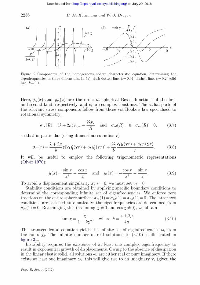
Figure 2. Components of the homogeneous sphere characteristic equation, determining theeigenfrequencies in three dimensions. In (b), dash-dotted line, k = 0.04; dashed line, k = 0.2; solidline, k = 0.1.

Here, jm(x) and ym(x) are the order-m spherical Bessel functions of the firstand second kind, respectively, and ci are complex constants. The radial parts ofthe relevant stress components follow from these via Hooke’s law specialized torotational symmetry:

srr(R) = (l + 2m)vr ,R + 2lvr

Rand srq(R) = 0, sr4(R) = 0, (3.7)

so that in particular (using dimensionless radius r)

srr(r) = l + 2m

bc[c1j ′

1(cr) + c2 y ′1(cr)] + 2l

bc1j1(cr) + c2y1(cr)

r. (3.8)

It will be useful to employ the following trigonometric representations(Olver 1970):

j1(x) = sin xx2

− cos xx

and y1(x) = −cos xx2

− sin xx

. (3.9)

To avoid a displacement singularity at r = 0, we must set c2 = 0.Stability conditions are obtained by applying specific boundary conditions to

determine the corresponding infinite set of eigenfrequencies. We enforce zerotractions on the entire sphere surface: srr(1) = srq(1) = sr4(1) = 0. The latter twoconditions are satisfied automatically; the eigenfrequencies are determined fromsrr(1) = 0. Rearranging this (assuming c �= 0 and cos c �= 0), we obtain

tan c = c

1 − kc2, where k = l + 2m

4m. (3.10)

This transcendental equation yields the infinite set of eigenfrequencies ui fromthe roots ci . The infinite number of real solutions to (3.10) is illustrated infigure 2a.

Instability requires the existence of at least one complex eigenfrequency toresult in exponential growth of displacements. Owing to the absence of dissipationin the linear elastic solid, all solutions ui are either real or pure imaginary. If thereexists at least one imaginary ui , this will give rise to an imaginary ci (given the





(a) (b)

a b

a

b

lI, mIlI, mIlII, mII lII, mII

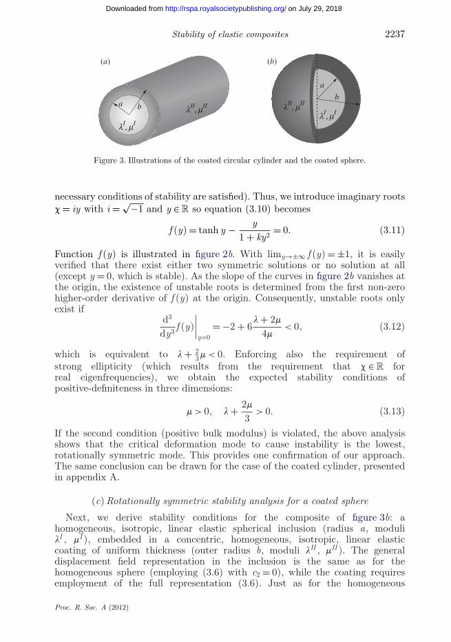
Figure 3. Illustrations of the coated circular cylinder and the coated sphere.

necessary conditions of stability are satisfied). Thus, we introduce imaginary rootsc = iy with i = √−1 and y ∈ R so equation (3.10) becomes

f (y) = tanh y − y1 + ky2

= 0. (3.11)

Function f (y) is illustrated in figure 2b. With limy→±∞ f (y) = ±1, it is easilyverified that there exist either two symmetric solutions or no solution at all(except y = 0, which is stable). As the slope of the curves in figure 2b vanishes atthe origin, the existence of unstable roots is determined from the first non-zerohigher-order derivative of f (y) at the origin. Consequently, unstable roots onlyexist if

d3

dy3f (y)

∣∣∣∣y=0

= −2 + 6l + 2m

4m< 0, (3.12)

which is equivalent to l + 23m < 0. Enforcing also the requirement of

strong ellipticity (which results from the requirement that c ∈ R forreal eigenfrequencies), we obtain the expected stability conditions ofpositive-definiteness in three dimensions:

m > 0, l + 2m

3> 0. (3.13)

If the second condition (positive bulk modulus) is violated, the above analysisshows that the critical deformation mode to cause instability is the lowest,rotationally symmetric mode. This provides one confirmation of our approach.The same conclusion can be drawn for the case of the coated cylinder, presentedin appendix A.

(c) Rotationally symmetric stability analysis for a coated sphere

Next, we derive stability conditions for the composite of figure 3b: ahomogeneous, isotropic, linear elastic spherical inclusion (radius a, modulilI , mI ), embedded in a concentric, homogeneous, isotropic, linear elasticcoating of uniform thickness (outer radius b, moduli lII , mII ). The generaldisplacement field representation in the inclusion is the same as for thehomogeneous sphere (employing (3.6) with c2 = 0), while the coating requiresemployment of the full representation (3.6). Just as for the homogeneous





sphere (and the two-dimensional cylinder, cf. appendix A), the angularcomponents of the displacement and traction conditions will not contributeto the stability conditions. Thus, we again need to analyse only the radialcomponents. The radial displacement components in inclusion and coating are(employing (3.9)), respectively,

vIr (r) = c1

[sin(c1r)

c21 r2

− cos(c1r)c1r

](3.14a)

and

vIIr (r) = d1

[sin(c2r)

c22r2

− cos(c2r)c2r

]− d2

[cos(c2r)

c22r2

+ sin(c2r)c2r

](3.14b)

with

ci =√

ru2b2

li + 2mi(3.15)

and material properties of inclusion (i = I ) and matrix (i = II ). We againdefine r = R/b ∈ [0, 1] with b the outer coating radius, x = a/b, and stressesare again obtained from the displacement fields via Hooke’s law. We imposeboundary conditions of zero tractions on the entire outer surface and continuityof displacements and tractions across the inclusion/coating interface:

sIIrr(1) = 0, sII

rr(x) = sIrr(x), vII

r (x) = vIr (x). (3.16)

Introducing the dimensionless quantities

k1 =√

mI

lI + 2mI, k2 =

√mII

lII + 2mII, k =

√lI + 2mI

lII + 2mII, j =

√ru2b2

lI + 2mI,

(3.17)the system (3.16) becomes

− c1

[sin(jx)j2x2

− cos(jx)jx

]+ d1

[sin(jkx)j2k2x2

− cos(jkx)jkx

]

− d2

[cos(jkx)j2k2x2

+ sin(jkx)jkx

]= 0, (3.18a)

d1

[4k2

2cos(jk)j2k2

+(

1jk

− 4k22

j3k3

)sin(jk)

]

+ d2

[4k2

2sin(jk)j2k2

−(

1jk

− 4k22

j3k3

)cos(jk)

]= 0 (3.18b)

and − c1k[4k2

1cos(jx)j2x2

+(

1jx

− 4k21

j3x3

)sin(jx)

]

+ d1

[4k2

2cos(jkx)j2k2x2

+(

1jkx

− 4k22

j3k3x3

)sin(jkx)

]

+ d2

[4k2

2sin(jkx)j2k2x2

−(

1jkx

− 4k22

j3k3x3

)cos(jkx)

]= 0. (3.18c)





We assume the same mass density for both materials; different densitiesalter the exact solutions but not the stability results (Kochmann & Drugan2009; Kochmann in press). Equations (3.18) are written in matrix formas M · (c1, d1, d2)T = 0, where M is the corresponding coefficient matrix;non-trivial solutions require detM = 0. This is the characteristic equation to besolved for the infinite set of eigenfrequencies ui (i.e. one solves for the infinite set ofsolutions ji). Employing a numerical search algorithm for the roots of detM = 0,we numerically determine whether or not imaginary roots u exist, and we candetermine those moduli and radii combinations that allow for imaginary andhence unstable eigenfrequencies, in order to obtain the complete stability map(for positive-definite coating moduli).

A closed-form analytical representation of the stability conditions can beobtained for the case when the inclusion violates positive-definiteness, while thecoating remains positive-definite. Stability is lost when at least one imaginarysolution j exists that solves the characteristic equation detM (j) = 0. In directanalogy to the homogeneous cylinder discussed in the appendix, such animaginary solution will exist only if the slope of the characteristic equation isnon-zero at the origin; thus, the boundary between stable and unstable regimesis found from the requirement that the characteristic equation’s slope vanishesat the origin, i.e. with y ∈ R,

limy→0

ddy

detM (iy) = 0. (3.19)

Let us introduce the parametrization lI = − 23(1 + 2b)mI , where b ∈ [0, 1] is

a dimensionless parameter (Drugan 2007). b = 0 corresponds to positive-definiteness and b = 1 to strong ellipticity, so b ∈ [0, 1] covers the full range ofinterest. One can show that (3.19) is satisfied when

lII

mII= −2

31 − b(mI /mII ) − (a/b)3(1 + 2b(mI /mII ))

1 − (a/b)3 − b(mI /mII ), (3.20)

which is the analytical expression of the stability limiting curve (i.e. replacing =by > ensures stability).

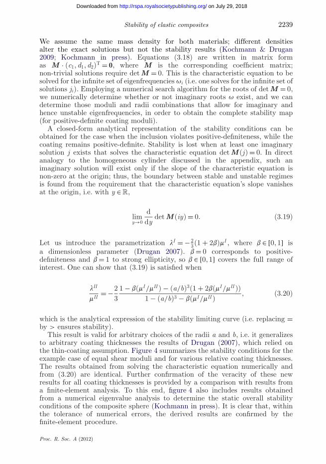
This result is valid for arbitrary choices of the radii a and b, i.e. it generalizesto arbitrary coating thicknesses the results of Drugan (2007), which relied onthe thin-coating assumption. Figure 4 summarizes the stability conditions for theexample case of equal shear moduli and for various relative coating thicknesses.The results obtained from solving the characteristic equation numerically andfrom (3.20) are identical. Further confirmation of the veracity of these newresults for all coating thicknesses is provided by a comparison with results froma finite-element analysis. To this end, figure 4 also includes results obtainedfrom a numerical eigenvalue analysis to determine the static overall stabilityconditions of the composite sphere (Kochmann in press). It is clear that, withinthe tolerance of numerical errors, the derived results are confirmed by thefinite-element procedure.





–1.4 –1.2 –1.0 –0.8 –0.6

1

2

3

4

t/a = 50% stable

unstable

t/a = 40%t/a = 30%

t/a = 20% t/a = 10% t/a = 5%t/a = 2%

t/a = 1%

lII/mII

lI/mI

Figure 4. Stability limit of the coated sphere for various relative coating thicknesses: comparison ofthe analytical solution (3.20) obtained from the present dynamic approach with the sufficientconditions of static stability obtained via the finite-element procedure. For each curve, thestable region lies above and to the right of the curve. Solid lines, dynamic analysis; crosses,finite-element method.

4. Static stability conditions for composites

(a) Stability conditions from overall elastic moduli

Thus far, we have shown for two specific composite geometries, via detaileddynamic analyses, that an inclusion material violating positive-definiteness canbe stabilized by the surrounding matrix material. We were fortunately able,in these basic geometries, to extract closed-form analytical statements of thestability requirements. For geometrically more complex composites, the stabilityanalysis method of choice would appear to be the numerical finite-elementapproach summarized at the end of §2. This alone would, of course, provideonly numerical stability results. We now introduce a method to determine closed-form analytical composite stability requirements for more geometrically complexcomposite materials, to be used in conjunction with the numerical finite-elementapproach. This is accomplished by deriving the relationship between overallstability and overall stiffness.

The bulk modulus k of an elastic medium, a scalar measure of the body’sresistance to volumetric changes, is defined in general by

k = VvpvV

, (4.1)

where p denotes the outward hydrostatic pressure acting on the surface of a bodyof volume V . For a composite of volume V with stress s and strain 3 that varyin its interior, one introduces the volumetric averages (X denoting position)

s = 1V

∫V

s(X) dv and 3 = 1V

∫V

3(X) dv, (4.2)

so that the bulk modulus of an infinitesimally strained composite can be writtenas (with d the dimension, and trT = Tii the trace of a tensor)

k = 1d

tr s

tr 3. (4.3)





Note that for anisotropic solids this defines a structural bulk modulus, whereasfor overall isotropic solids, this definition yields the effective linear elastic bulkmodulus of the composite. Recall that, with DV being the change in volume,

V tr 3 =∫V

tr 3 dv =∫V

tr(gradu) dv =∫V

divu dv = DV . (4.4)

With Gauss’ theorem and equilibrium without body forces (divs = 0), wetransform the integral for the average stress into a surface integral over vV :

∫V

tr sdv = tr∫V

s dv = tr(∫

vVt ⊗ X ds

)=

∫vV

t · X ds (4.5)

with t = sn denoting the surface traction. When a uniform outward hydrostaticpressure p acts on the entire surface, t = (pI )n = pn on the surface. Then,

V tr s =∫V

tr sdv = p∫

vVn · Xds = p

∫V

divX dv = pdV . (4.6)

Hence, the overall effective bulk modulus of the body subject to a constant p is

k = 1d

pdDV /V

= pVDV

. (4.7)

Next, we link the bulk modulus to the stability of the body. The elastic energystored in a deformed, linear elastic solid is

I = 12

∫V

3 : s dv = 12

∫V

3 : C : 3 dv. (4.8)

As we assume no body forces act, the total work P performed on the body is duesolely to the constant, outward external pressure p:

P =∫

vVu · t ds = p

∫vV

u · n ds = p∫V

divu dv = pDV . (4.9)

When the deformed body under hydrostatic pressure is in equilibrium, thendP = dI and consequently P = I + const. Here, we assume the unstrained body(3 = 0) to be in equilibrium, so that the constant must vanish. Therefore, weconclude that

12

∫V

3 : C : 3 dv = pDV . (4.10)

Stability of a deformed linear elastic solid subject to infinitesimal strain andstress requires that the stored energy be positive for any non-zero kinematicallyadmissible strain field 3 (Pearson 1956; Hill 1957). Applied to the equilibriumconfiguration, stability requires

12

∫V

3 : C : 3 dv > 0 ⇒ pDV > 0. (4.11)

For a constant pressure p, stability hence implies that p and the volume changemust always be of the same sign. Therefore, it follows from (4.7) that a linear





elastic solid in stable equilibrium must exhibit a positive overall (effective) bulkmodulus:

k > 0 for stability. (4.12)

Our reasoning is sufficiently general for any linear elastic solid: no assumptionswere made about isotropy or any other specific form of the elastic modulustensor, nor about the geometry of the body (except that it be continuousand simply connected). However, this result is not bijective: a positive bulkmodulus does not generally guarantee stability for the following reason. The firstinequality in (4.11) must hold for arbitrary non-zero kinematically admissible3 for overall stability; a positive bulk modulus, however, only ensures that theintegral is positive for the equilibrium configuration and not for any perturbationin general. What this means is that, if a rigorous (e.g. numerical) stability analysisshows a heterogeneous linear elastic body to be in stable equilibrium, analyticalrequirements for this stability can be obtained from the condition that the body’soverall bulk modulus be positive. We will demonstrate this concept in §5, wherewe derive analytical sufficient stability conditions for example composites andconfirm their validity. Furthermore, we conclude that (4.12) is necessary foroverall composite stability; our proposed approach for geometrically complexcomposites is to verify its sufficiency by application of a numerical finite-elementapproach. We will discuss the implications for general composites in §4b andillustrate the concept explicitly for a periodic matrix/inclusion composite in §5c.

We note in passing that application of (4.12) to the simple specific casesof negative-stiffness-phase composites analysed here shows that, in these cases,as the inclusion bulk modulus is tuned to increasingly negative values, theoverall composite will go unstable before infinite composite bulk modulus canbe attained. Whether this is true for general composites is still an open question;our research in progress shows that other material properties can attain positiveextreme values owing to negative inclusion bulk modulus while retaining overall(composite) stability.

For completeness, we also investigate the effect of pre-stress on compositestability. For any infinitesimal pre-stress s0, the above energy method can bemodified to yield

I = 12

∫V

3 : (C : 3 + 2s0) dv,

andP =

∫vV

u · (t + s0 · n) ds = p∫V

divu dv +∫V

3 : s0 dv,

so that (4.10) remains unaltered and the final conclusions are the same.

(b) Stability conditions from effective elastic moduli

The geometrical and topological details of actual composite materials areof enormous complexity and often span multiple length scales. For mostcomposites in engineering applications, there exists a considerable distinctionbetween the body’s macroscale (i.e. the length scale of the body’s outerextensions or its geometrical shape) and its microscale (i.e. the length scale ofall microstructural characteristics, e.g. the average diameter of inclusions in aparticle-matrix composite). As a consequence, it is legitimate to assume a clear





n × n macrostructure(matrix with n × n inclusions)

elementaryunit cell

m × m unit cellmacrostructure

periodicmicrostructure

(a) (b)

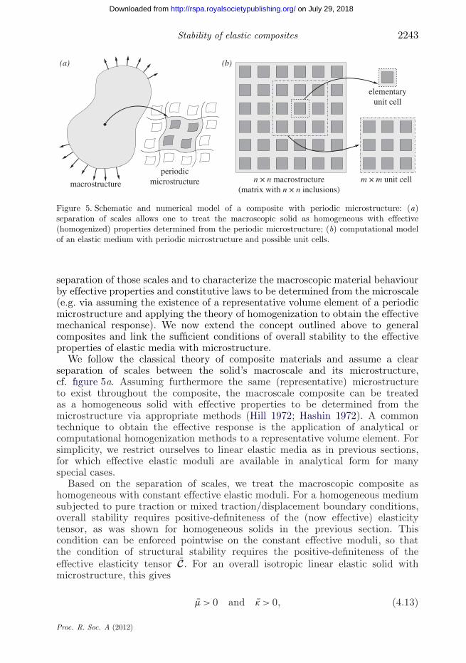
Figure 5. Schematic and numerical model of a composite with periodic microstructure: (a)separation of scales allows one to treat the macroscopic solid as homogeneous with effective(homogenized) properties determined from the periodic microstructure; (b) computational modelof an elastic medium with periodic microstructure and possible unit cells.

separation of those scales and to characterize the macroscopic material behaviourby effective properties and constitutive laws to be determined from the microscale(e.g. via assuming the existence of a representative volume element of a periodicmicrostructure and applying the theory of homogenization to obtain the effectivemechanical response). We now extend the concept outlined above to generalcomposites and link the sufficient conditions of overall stability to the effectiveproperties of elastic media with microstructure.

We follow the classical theory of composite materials and assume a clearseparation of scales between the solid’s macroscale and its microstructure,cf. figure 5a. Assuming furthermore the same (representative) microstructureto exist throughout the composite, the macroscale composite can be treatedas a homogeneous solid with effective properties to be determined from themicrostructure via appropriate methods (Hill 1972; Hashin 1972). A commontechnique to obtain the effective response is the application of analytical orcomputational homogenization methods to a representative volume element. Forsimplicity, we restrict ourselves to linear elastic media as in previous sections,for which effective elastic moduli are available in analytical form for manyspecial cases.

Based on the separation of scales, we treat the macroscopic composite ashomogeneous with constant effective elastic moduli. For a homogeneous mediumsubjected to pure traction or mixed traction/displacement boundary conditions,overall stability requires positive-definiteness of the (now effective) elasticitytensor, as was shown for homogeneous solids in the previous section. Thiscondition can be enforced pointwise on the constant effective moduli, so thatthe condition of structural stability requires the positive-definiteness of theeffective elasticity tensor C. For an overall isotropic linear elastic solid withmicrostructure, this gives

m > 0 and k > 0, (4.13)





where m and k are the effective shear and bulk moduli, respectively. Therefore,knowledge of the effective elastic properties (for overall isotropic compositesof arbitrary geometry) is, in principle, sufficient to obtain the conditions ofoverall stability (but see provisos in the next paragraph). For any compositemodel, the effective shear modulus will depend on the constituent shear moduli,and the necessary condition of stability requires (pointwise) strong ellipticityof each constituent. Hence, the individual shear moduli must be positive forstability, so the first condition in (4.13) is generally satisfied automatically.The second condition thus becomes the critical stability condition which, again,requires the effective, overall bulk modulus to be positive for stability. This wasalready found in the previous section for macroscopic composites of arbitrarygeometry, cf. equation (4.12). Here, we conclude that the same condition ofstability also applies to general composites with microstructure when replacingthe overall elastic properties by the effective (homogenized) ones. In multi-cell materials, cooperative phenomena can affect the overall stability of thesolid. Therefore, it is imperative to check stability by two criteria: (i) thelocal (pointwise) material stability (which only detects periodic phenomena onthe level of the representative volume element) and (ii) the structural (global)stability of the structure or solid (which detects long-range instabilities orlocalization phenomena). Therefore, we must also check macroscopic stability,i.e. we interpret (4.13) as necessary conditions of stability that can be employedto derive closed-form analytical stability conditions whose sufficiency is to beverified by, e.g. a finite-element study.

Note that this approach only applies to composites whose entire surface phasehas positive-definite elastic moduli. In the cases of a non-positive-definite coating,this coating material (comprising the outer free surface of the composite) willalways cause global instability (this can be seen explicitly in the coated cylindercomposite via the general analysis of Kochmann & Drugan 2009).

5. Analytical stability conditions from effective bulk moduli

The conclusion that composite stability requires a positive overall bulk modulusis perhaps unsurprising in light of the known homogeneous material stabilityrequirements, yet it facilitates an elegant and alternative derivation of the staticcomposite stability conditions in a closed form. We now confirm the veracityof this approach via three specific examples. First, we employ (4.12) to deriveclosed-form conditions of static stability for the examples of coated cylinder andsphere directly from the overall bulk modulus. Then, we use (4.13) to derive ananalytical sufficient condition of static stability for a geometrically more complexmatrix/inclusion composite.

(a) Coated cylinder

The overall bulk modulus of the coated cylinder shown in figure 3a is

k = x2(lI − lII + mI − mII )mII + (lII + mII )(lI + mI + mII )lI + mI + mII − x2(lI − lII + mI − mII )

, (5.1)





with x = a/b and mi , li the elastic moduli of inclusion (I ) and coating (II ).Stability conditions follow from requiring k > 0, which admits two possiblesolutions; the one giving the correct stability requirement is

lI >−(mII + lII )(mII + mI ) + mII (mII + lII − mI )x2

lII + mII (1 + x2). (5.2)

The other solution is discarded because, when violating positive-definiteness, theoverall bulk modulus first becomes negative, which is the stability limit sought;it later returns to positive values, to which the discarded inequality corresponds.

The necessary conditions of pointwise stability require mI , mII ≥ 0. Thecomposite is stable overall if both phases are positive-definite, i.e. if li + mi > 0for both materials. The range of interest hence reduces to those cases where theinclusion violates positive-definiteness but still satisfies the necessary conditionsof strong ellipticity. Therefore, it is convenient to make use of the dimensionlessparameter b to define lI = −(1 + b)mI (Drugan 2007): b = 0 corresponds topositive-definiteness and b = 1 to strong ellipticity, so b ∈ [0, 1] covers the fullrange of interest. Inserting lI = −(1 + b)mI into (5.2) along with the necessaryconditions of stability and x ≤ 1, we find the following sufficient conditions ofoverall stability:

mII >b mI

1 − x2∧ lII > −mII − bmI − x2(mII + bmI )

mII (1 − x2) − bmImII , b ∈ [0, 1]. (5.3)

Equations (5.3) give new sufficient conditions for stability of the coated cylinderfor all coating thicknesses in a closed form; they agree exactly with thosedetermined numerically by Kochmann & Drugan (2009). Furthermore, theyreduce exactly to those derived by Drugan (2007) for a thin coating by definingthe coating thickness t as b = a + t, so that x = a/(a + t) and assuming t/a 1.The complete set of sufficient conditions in dimensionless form both for the fullrange of coating thicknesses and for the thin-coating approximation is

mI > 0,lI

mI> −(1 + b) with b ∈ [0, 1],

mII

mI>

b

1 − ( ab )2

t/a→0−→ b

2at

andlII

mII> −

1 − b mI

mII − ( ab )2(1 + b mI

mII )

1 − ( ab )2 − b mI

mII

t/a→0−→ −1 − b a

tmI

mII (1 + ta )

1 − b

2at

mI

mII

.

Appendix A shows the dynamic approach yields identical conditions.The present analysis also permits derivation of the sufficient stability

conditions for a dilute particle/matrix composite by investigating the limit oflarge coating thicknesses b: taking the limit of a/b → 0 in the above solution yields

mI > 0, mII > 0, lI + mI > −{

mI , if mI < mII

mII , if mI ≥ mII , lII + mII > 0. (5.4)





The fourth condition requires the coating merely to be positive-definite, whereasthe third condition allows the inclusion to violate positive-definiteness, with thestable regime for the inclusion moduli increasing with increasing shear stiffnessof the coating material. In particular, for mII ≥ mI , the stability conditions for theinclusion reduce to those of strong ellipticity.

(b) Coated sphere

The same method is applied to a coated sphere, whose overall bulk modulus is

k = 4x3(3lI − 3lII + 2mI − 2mII )mII + (3lII + 2mII )(3lI + 2mI + 4mII )3x3(3lII − 3lI + 2mII − 2mI ) + 3(3lI + 2mI + 4mII )

.

The complete set of sufficient conditions for the full range of coating thicknessesand for the thin-coating approximation is

mI > 0,lI

mI> −2

3(1 + 2b) with b ∈ [0, 1],

mII

mI> b

11 − ( a

b )3

t/a→0−→ b

3at

andlII

mII> −2

3

1 − b mI

mII − ( ab )3(1 + 2b mI

mII )

1 − ( ab )3 − b mI

mII

t/a→0−→ −23

1 − b at

mI

mII (1 − 2 ta )

1 − b

3at

mI

mII

.

These results give the sufficient conditions for static stability of the coatedsphere for all coating thicknesses in a closed form. They agree exactly with(3.20) determined from the dynamic analysis outlined in §3(c). They also coincidewith those of Drugan (2007) in the thin coating limit (t/a 1), except for thelower bound on mII /mI , for which Drugan (2007) derived the stronger restrictionmII /mI ≥ b a/t. As the present approach is valid for the full range of coatingthicknesses, the above results generalize those of Drugan (2007).

The sufficient stability conditions for the dilute composite in three dimensionsare obtained by taking the limit of a/b → 0 in the above solution:

mI > 0, mII > 0, lI + 23

mI > −43

{mI , if mI < mII

mII , if mI ≥ mII , lII + 23

mII > 0. (5.5)

Just as for the two-dimensional problem, the fourth condition requires the coatingto be merely positive-definite, while the third condition allows the inclusionto violate positive-definiteness, with the stable regime for the inclusion moduliincreasing with increasing shear stiffness of the coating material. For mII ≥ mI ,the stability conditions for the inclusion reduce to those of strong ellipticity.

(c) Solid with periodic microstructure

As a concrete example to confirm the conclusions of §4b for more generalcomposites, we apply our approach to an elastic two-phase composite with equalconstituent shear moduli m1 = m2 = m, bulk moduli k1 and k2 and volume fractions





v1 and v2, for which Hill (1963) derived the following exact results for the effectivemoduli for an isotropic composite (or one with cubic material symmetry) witharbitrarily shaped constituents:

m = m, k = 3k1k2 + 4mkV

3k1k2 + 4mkRkR, (5.6)

where kR and kV are the Reuss and Voigt bounds on the bulk modulus,respectively:

kR =(

v1

k1+ v2

k2

)−1

, kV = v1k1 + v2k2. (5.7)

Importantly, this result does not depend on a positive-definite strain energydensity: it also applies to negative constituent bulk moduli. Application ofconditions (4.13) directly gives the prospective (to be confirmed by a numericalfinite-element stability analysis) sufficient stability conditions for otherwisearbitrary overall isotropic or cubic two-phase composites whose entire surfaceborders the positive-definite phase:

m > 0, k1 > −4(1 − v1)mk2

3k2 + 4v1m. (5.8)

First, it is interesting to compare these sufficient stability conditions to thosederived in the previous section for a single coated-sphere composite which,rewritten in terms of shear and bulk moduli with equal sphere and coating bulkmodulus m > 0 (and k2 > 0), are:

k1 > −4[1 − (a/b)3]mk2

3k2 + 4(a/b)3m. (5.9)

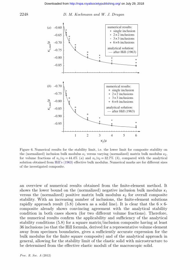
Since v1 = (a/b)3, conditions (5.9) and (5.8) exactly coincide.We now confirm that (5.8) are indeed sufficient stability conditions for a specific

sample of a matrix/distributed-inclusions composite material under zero-tractionboundary conditions via application of the numerical finite-element stabilityanalysis described earlier. The specific linear elastic composite consists of asquare matrix of positive-definite material containing a regular array of n × nidentical square non-positive-definite inclusions with equal spacing (to ensurecubic symmetry) that are fully encapsulated by the matrix material; see thelarge figure in figure 5b. Numerical results were obtained by investigating theeigenvalues of the full overall stiffness matrix (which corresponds to zero-tractionboundary conditions on the entire outer surface of the constructed composite).The sought stability limit is found when the first negative eigenvalue arises. Thisprocedure is repeated for composite samples with increasing numbers of inclusions(specifically, we compute results for n = 1, 2, 3, 6). To permit a comparison withthe analytical conditions (5.8), the shear moduli of inclusion and matrix materialare chosen to be equal. Furthermore, note that, for comparison with the two-dimensional (plane strain) finite-element model, Hill’s result must be modifiedby using the plane strain bulk moduli of the composite phases. Figure 6 gives





–0.85

–0.80

–0.75

–0.70

–0.65

–0.60(a)

(b)

single inclusion

analytical solution:

numerical results:

after Hill (1963)

1 2 3 4 5 6

–0.95

–0.90

–0.85

–0.80

–0.75

–0.70

6 × 6 inclusions3 × 3 inclusions2 × 2 inclusions

6 × 6 inclusions3 × 3 inclusions2 × 2 inclusions

single inclusion

analytical solution:

numerical results:

after Hill (1963)

k 1,m

in/m

k 1,m

in/m

k2/m

Figure 6. Numerical results for the stability limit, i.e. the lower limit for composite stability onthe (normalized) inclusion bulk modulus k1 versus varying (normalized) matrix bulk modulus k2,for volume fractions of v1/v2 = 44.4% (a) and v1/v2 = 32.7% (b), compared with the analyticalsolution obtained from Hill’s (1963) effective bulk modulus. Numerical marks are for different sizesof the investigated composite.

an overview of numerical results obtained from the finite-element method. Itshows the lower bound on the (normalized) negative inclusion bulk modulus k1versus the (normalized) positive matrix bulk modulus k2 for overall compositestability. With an increasing number of inclusions, the finite-element solutionsrapidly approach result (5.8) (shown as a solid line). It is clear that the 6 × 6-composite already shows convincing agreement with the analytical stabilitycondition in both cases shown (for two different volume fractions). Therefore,the numerical results confirm the applicability and sufficiency of the analyticalstability conditions (5.8) for a square matrix/inclusion composite having at least36 inclusions (so that the Hill formula, derived for a representative volume elementaway from specimen boundaries, gives a sufficiently accurate expression for thebulk modulus for the finite square composite) and of the analytical approach ingeneral, allowing for the stability limit of the elastic solid with microstructure tobe determined from the effective elastic moduli of the macroscopic solid.





6. Conclusions

We have presented methods to derive closed-form analytical conditions ofstatic and kinematic stability for elastic composites and multi-phase solidshaving a negative-stiffness phase, which demonstrate the expanded regime ofstability owing to the geometric constraints enforced by appropriately placedpositive-definite phases. We have applied these methods to the fundamentalcomposites of coated cylinder and coated sphere, for all coating thicknesses,and thereby confirmed and generalized those stability conditions previouslyavailable. Furthermore, an analogous method has been outlined for solidswith microstructures and its applicability was illustrated by deriving closed-form analytical stability requirements for a specific matrix/distributed-inclusionscomposite, which were confirmed by a numerical finite-element stability analysis.Our results provide closed-form analytical stability requirements crucial to theexploration and development of novel, stable negative-stiffness-phase compositematerials tuned to exhibit extreme properties.

This research was supported by the National Science Foundation (NSF) under grant DMR-0949254,and the Army Research Office/Defense Advanced Research Projects Agency (ARO/DARPA) undergrant 57492-EG-DRP.

Appendix A. Dynamic stability analysis in plane strain

(a) Rotationally symmetric stability analysis for a homogeneous cylinder

Analogously to the derivation in §3, the displacement components for rotationalsymmetry in plane strain can be written in the separable form (where the realpart of the right sides is implied)

ur(R, t) = vr(R) eiut and uq(R, t) = vq(R) eiut (A 1)

using polar coordinates (R, q). Applying this to the dynamic governing equationsabsent body forces, we arrive at the uncoupled Navier equations for plane strain

R2v′′r + Rv′

r +[

ru2R2

l + 2m− 1

]vr = 0 (A 2)

and

R2v′′q + Rv′

q +[

ru2R2

m − 1

]vq = 0. (A 3)

Using dimensionless radius r = R/b ∈ [0, 1] with b the outer radius of thecircular cylinder, the general solution representations for the radial parts of thedisplacement components are

vr(r) = c1J1(cpr) + c2Y1(cpr), vq(r) = c3J1(csr) + c4Y1(csr) (A 4)

with

cp =√

ru2b2

l + 2mand cs =

√ru2b2

m. (A 5)





–5 –2.5 2.5 5 7.5 10

–8–6–4–2

2

J1(c)/J0(c)

I1(y)/I0(y) – (1 + k)y(1 + l/2m) c

468

y

(a) (b)

–6 –4 –2 2 4 6

–4

–2

2

4

c

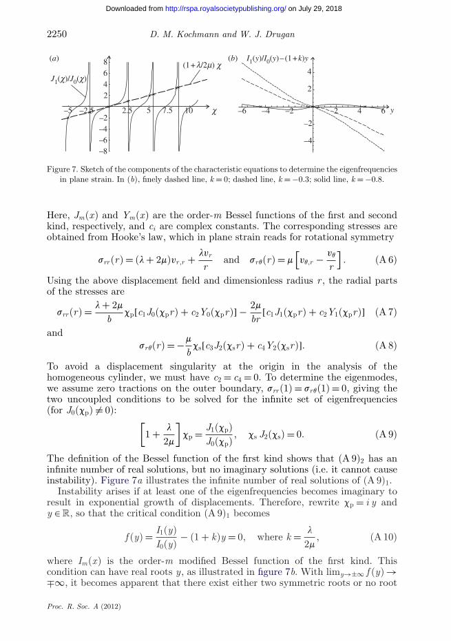
Figure 7. Sketch of the components of the characteristic equations to determine the eigenfrequenciesin plane strain. In (b), finely dashed line, k = 0; dashed line, k = −0.3; solid line, k = −0.8.

Here, Jm(x) and Ym(x) are the order-m Bessel functions of the first and secondkind, respectively, and ci are complex constants. The corresponding stresses areobtained from Hooke’s law, which in plane strain reads for rotational symmetry

srr(r) = (l + 2m)vr ,r + lvr

rand srq(r) = m

[vq,r − vq

r

]. (A 6)

Using the above displacement field and dimensionless radius r , the radial partsof the stresses are

srr(r) = l + 2m

bcp[c1J0(cpr) + c2Y0(cpr)] − 2m

br[c1J1(cpr) + c2Y1(cpr)] (A 7)

andsrq(r) = −m

bcs[c3J2(csr) + c4Y2(csr)]. (A 8)

To avoid a displacement singularity at the origin in the analysis of thehomogeneous cylinder, we must have c2 = c4 = 0. To determine the eigenmodes,we assume zero tractions on the outer boundary, srr(1) = srq(1) = 0, giving thetwo uncoupled conditions to be solved for the infinite set of eigenfrequencies(for J0(cp) �= 0): [

1 + l

2m

]cp = J1(cp)

J0(cp), cs J2(cs) = 0. (A 9)

The definition of the Bessel function of the first kind shows that (A 9)2 has aninfinite number of real solutions, but no imaginary solutions (i.e. it cannot causeinstability). Figure 7a illustrates the infinite number of real solutions of (A 9)1.

Instability arises if at least one of the eigenfrequencies becomes imaginary toresult in exponential growth of displacements. Therefore, rewrite cp = i y andy ∈ R, so that the critical condition (A 9)1 becomes

f (y) = I1(y)I0(y)

− (1 + k)y = 0, where k = l

2m, (A 10)

where Im(x) is the order-m modified Bessel function of the first kind. Thiscondition can have real roots y, as illustrated in figure 7b. With limy→±∞ f (y) →∓∞, it becomes apparent that there exist either two symmetric roots or no root





at all (except y = 0, which is stable). To determine the condition of stability,we must identify those combinations of the elastic moduli for which roots exist.From the limits at ±∞, we infer that roots exist only if f ′(0) > 0, giving thestability condition

ddy

f (y)∣∣∣∣y=0

< 0. (A 11)

Along with the necessary conditions, m > 0 and l + 2m > 0 (which are apparentfrom the definitions of cp and cs) we hence deduce the stability conditions

m > 0, l + m > 0, (A 12)

the expected conditions of elastic moduli positive-definiteness in two dimensions.

(b) Rotationally symmetric stability analysis for a coated cylinder

Based on the previous analysis, we now derive the stability conditions for thecoated cylinder of figure 3a, which consists of a homogeneous, isotropic, linearelastic inclusion (radius a, elastic moduli lI and mI ) and a homogeneous, isotropic,linear elastic coating (outer radius b, moduli lII and mII ). The radial part of thegeneral solution for the inclusion is the same as above (i.e. with the Bessel-Yterms being omitted)

vIr (r) = c1J1(cI

pr) and vIq (r) = c2J1(cI

s r), (A 13)

while the solution in the coating material requires the full representation

vIIr (r) = d1J1(cII

p r) + d2Y1(cIIp r), vII

q (r) = d3J1(cIIs r) + d4Y1(cII

s r) (A 14)

with

cip =

√riu2b2

li + 2mi, ci

s =√

riu2b2

mi, (A 15)

with the respective material properties of inclusion (superscript I ) and matrix(II ). As before, we employ the dimensionless radius r = R/b ∈ [0, 1] with b theouter radius of the cylindrical body, and a the radius of the inclusion. Weintroduce the dimensionless radius ratio x = a/b. The stresses are obtained fromthe displacement fields in the same manner as for the homogeneous solid.

We investigate the case of zero tractions on the outer boundary, and we enforcecontinuity of displacements and of tractions across the interface between inclusionand coating. This gives the following system of six equations:

sIIrr(1) = 0, sII

rq(1) = 0,

sIIrr(x) = sI

rr(x), sIIrq(x) = sI

rq(x)

and vIIr (x) = vI

r (x), vIIq (x) = vI

q (x).

Note that, as for the homogeneous body, the radial and angular components of thedisplacements and tractions are independent, i.e. the above set of six equationscan be reduced to two independent sets of three equations each (one system ofequations involving constants c1, d1, d2 and one set involving c2, d3, d4). This willbe beneficial for the determination of the unstable eigenfrequencies.





For brevity, we use abbreviations (3.17). With these dimensionless variables,the two systems of equations assume the following forms. The first system ofequations stems from continuity of vr and srr , and zero tractions srr on theboundary:

− c1J1(jx) + d1J1(kjx) + d2Y1(kjx) = 0,

d1[kjJ0(kj) − 2k22J1(kj)] + d2[kjY0(kj) − 2k2

2Y1(k j)] = 0

and d1

[kjJ0(kjx) − 2k2

2J1(kjx)x

]+ d2

[kjY0(kjx) − 2k2

2Y1(kjx)x

]

− c1k2[jJ0(jx) − 2k2

1J1(jx)x

]= 0.

The second system of equations results from continuity of vq and srq, and zerotractions srq on the boundary:

− c2J1

(jxk1

)+ d3J1

(kjxk2

)+ d4Y1

(kjxk2

)= 0,

d3J2

(kjk2

)+ d4Y2

(kjk2

)= 0

and − c2

(k1

k2

)2

kJ2

(jxk1

)+ d3J2

(kjxk2

)+ d4Y2

(kjxk2

)= 0.

In matrix form, where M i are the corresponding coefficient matrices, we have

M 1 · (c1, d1, d2)T = 0, M 2 · (c2, d3, d4)T = 0, (A 16)

which indicates that non-trivial solutions exist if

detM = detM 1 · detM 2 = 0. (A 17)

This is the characteristic equation to be solved for the infinite setof eigenfrequencies u. One finds that detM 2 = 0 only yields real-valuedeigenfrequencies. We numerically determine whether or not imaginary roots j = iy(y ∈ R) exist and construct the complete stability map (for positive-definitematrix moduli). The results are identical to those obtained from the full analysis(Kochmann & Drugan 2009) (figure 8).

Just as for the coated sphere, we can obtain a closed-form analytical expressionfor the stability limit by defining lI = −(1 + b)mI and evaluating equation (3.19)for matrix M 1 of the present formulation. This yields the stability limit as

lII

mII= −

1 − b mI

mII − ( ab )2(1 + b mI

mII )

1 − ( ab )2 − b mI

mII

, (A 18)

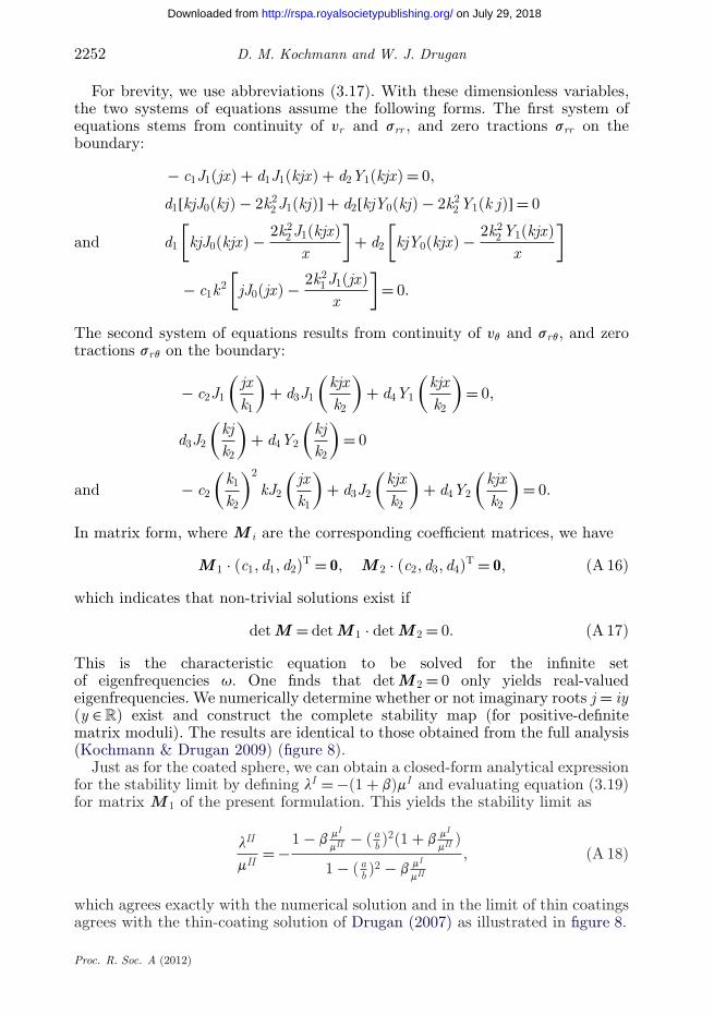
which agrees exactly with the numerical solution and in the limit of thin coatingsagrees with the thin-coating solution of Drugan (2007) as illustrated in figure 8.





–1.35 –1.30 –1.25 –1.20 –1.15 –1.10 –1.05

–1.0

–0.5

0.5

1.0

1.5

2.0

–1.00

t/a = 1%

t/a = 2%

t/a = 5%t/a = 10%

t/a = 20%

t/a = 30%

stable

unstable

lII/mII

lI/mI

Figure 8. Comparison of the stability limit for various coating thicknesses as obtained from thepresent, rotational symmetric formulation (which coincides with solutions from the full analysis ofKochmann & Drugan (2009)) and from the analytical thin-coating solution (Drugan 2007) for thecoated cylinder. For each curve, the stable region lies above and to the right of the curve. Dottedlines, Drugan (2007); solid lines, this work.

References

Drugan, W. J. 2007 Elastic composite materials having a negative stiffness phase can be stable.Phys. Rev. Lett. 98, 055502.

Hashin, Z. 1972 Analysis of composite materials—a survey. J. Appl. Mech. 50, 481–505.(doi:10.1115/1.3167081)

Hashin, Z. & Shtrikman, S. 1963 A variational approach to the theory of the elastic behaviour ofmultiphase materials. J. Mech. Phys. Solids 11, 127–140. (doi:10.1016/0022-5096(63)90060-7)

Hill, R. 1957 On uniqueness and stability in the theory of finite elastic strain. J. Mech. Phys. Sol.5, 229–241. (doi:10.1016/0022-5096(57)90016-9)

Hill, R. 1963 Elastic properties of reinforced solids—some theoretical principles. J. Mech. Phys.Solids 11, 357–372. (doi:10.1016/0022-5096(63)90036-X)

Hill, R. 1972 On constitutive macrovariables for heterogeneous solids at finite strain. Proc. R. Soc.Lond. A 326, 131–147. (doi:10.1098/rspa.1972.0001)

Jaglinski, T., Kochmann, D., Stone, D. & Lakes, R. S. 2007 Composite materials with viscoelasticstiffness greater than diamond. Science 315, 620–622. (doi:10.1126/science.1135837)

Kelvin, Lord, (Thomson, W.) 1888 On the reflection and refraction of light. Philos. Mag. 26,414–425.

Kirchhoff, G. 1859 Über das Gleichgewicht und die Bewegung eines unendlich dünnen elastischenStabes. J. Reine Angew. Math. 56, 285–313. (doi:10.1515/crll.1859.56.285)

Kochmann, D. M. In press. Stability criteria for elastic composites and the influence of geometryon the stability of a negative-stiffness phase. Phys. Stat. Sol. (doi:10.1002/pssb.201084213)

Kochmann, D. M. & Drugan, W. J. 2009 Dynamic stability analysis of an elastic composite materialhaving a negative-stiffness phase. J. Mech. Phys. Solids 57, 1122–1138. (doi:10.1016/j.jmps.2009.03.002)

Kochmann, D. M. & Drugan, W. J. 2011 Infinitely-stiff composite via a rotation-stabilized negative-stiffness phase. Appl. Phys. Lett. 99, 011909.

Koiter, W. T. 1965 Energy criterion of stability for continuous elastic bodies I and II. Proc. K.Ned. Akad. Wet. B—Phys. Sci. 68, 178–202.

Lakes, R. 1987 Foam structures with a negative Poisson’s ratio. Science 235, 1038–1040.(doi:10.1126/science.235.4792.1038)

Lakes, R. S. 2001 Extreme damping in compliant composites with a negative stiffness phase. Philos.Mag. Lett. 81, 95–100. (doi:10.1080/09500830010015332)



http://dx.doi.org/doi:10.1115/1.3167081

http://dx.doi.org/doi:10.1016/0022-5096(63)90060-7

http://dx.doi.org/doi:10.1016/0022-5096(57)90016-9

http://dx.doi.org/doi:10.1016/0022-5096(63)90036-X

http://dx.doi.org/doi:10.1098/rspa.1972.0001

http://dx.doi.org/doi:10.1126/science.1135837

http://dx.doi.org/doi:10.1515/crll.1859.56.285

http://dx.doi.org/doi:10.1002/pssb.201084213

http://dx.doi.org/doi:10.1016/j.jmps.2009.03.002

http://dx.doi.org/doi:10.1016/j.jmps.2009.03.002

http://dx.doi.org/doi:10.1126/science.235.4792.1038

http://dx.doi.org/doi:10.1080/09500830010015332



Lakes, R. S. & Drugan, W. J. 2002 Dramatically stiffer elastic composite materials due to a negativestiffness phase? J. Mech. Phys. Solids 50, 979–1009. (doi:10.1016/S0022-5096(01)00116-8)

Liu, Z., Chan, C. T. & Sheng, P. 2005 Analytic model of phononic crystals with local resonances.Phys. Rev. B 71, 014103. (doi:10.1103/PhysRevB.71.014103)

Lyapunov, A. M. 1966 Stability of motion. New York, NY: Academic Press.Mandel, J. 1962 Ondes plastique dans un milieu indéfini à trois dimensions. J. Mech. 1, 3–30.Mandel, J. 1966 Conditions de stabilité et postulat de Drucker. In Rheology and solid mechanics

(eds J. Kravtchenko & M. Sirieys), pp. 58–68. Berlin, Germany: Springer.Mary, T. A., Evans, J. S. O., Vogt, T. & Sleight, A. W. 1996. Negative thermal expansion from

0.3 to 1050 Kelvin in ZrW2O8. Science 5, 90–92.Milton, G. W. 2001 Theory of composites. Cambridge, UK: Cambridge University Press.Morrey, C. B. 1952 Quasi-convexity and the lower semicontinuity of multiple integrals. Pacific J.

Math. 2, 25–53.Olver, F. W. J. 1970 Bessel functions of integer order. In Handbook of mathematical functions (eds

M. Abramowitz & I. A. Stegun), NewYork, NY: Dover Inc.Paul, B. 1960 Prediction of elastic constants of multi-phase materials. Trans. AIME 218, 36–41.Pearson, C. E. 1956 General theory of elastic stability. Quart. Appl. Math. 14, 133–144.Reuss, A. 1929 Berechnung der Fließgrenze von Mischkristallen auf Grund der

Plastizitätsbedingung für Einkristalle. Z. Angew. Math. Mech. 9, 49–58. (doi:10.1002/zamm.19290090104)

Shelby, R. A., Smith, D. R. & Schultz, S. 2001 Experimental verification of a negative index ofrefraction. Science 292, 77–79. (doi:10.1126/science.1058847)

Voigt, W. 1889 Über die Beziehung zwischen den beiden Elastizitätskonstanten isotroper Körper.Wied. Ann. 38, 573–587.

Wang, Y. C. & Lakes, R. S. 2001 Extreme thermal expansion, piezoelectricity, and other coupledfield properties in composites with a negative stiffness phase. J. Appl. Phys. 90, 6458–6465.(doi:10.1063/1.1413947)

Wang, Y.-C. & Lakes, R. 2004 Negative stiffness-induced extreme viscoelastic mechanicalproperties: stability and dynamics. Phil. Mag. 84, 3785–3801. (doi:10.1080/1478643042000282702)

Wang, Y.-C. & Lakes, R. 2006 Stability of negative stiffness viscoelastic systems. Quart. Appl.Math. 63, 34–55.

Ziegler, H. 1953 Linear elastic stability. Zeitschr. Angewandt. Math. Phys. (ZAMP) 4, 89–121.(doi:10.1007/BF02067575)



http://dx.doi.org/doi:10.1016/S0022-5096(01)00116-8

http://dx.doi.org/doi:10.1103/PhysRevB.71.014103

http://dx.doi.org/doi:10.1002/zamm.19290090104

http://dx.doi.org/doi:10.1002/zamm.19290090104

http://dx.doi.org/doi:10.1126/science.1058847

http://dx.doi.org/doi:10.1063/1.1413947



http://dx.doi.org/doi:10.1007/BF02067575


Analytical stability conditions for elastic composite...

Documents

Transcript of Analytical stability conditions for elastic composite...