PhD Thesis - Analytical and numerical modelling of elastic ...
123
Faculty of Science and Engineering Department of Exploration Geophysics Analytical and Numerical Modelling of Elastic Properties of Isotropic and Anisotropic Rocks and Their Stress Dependencies Pavel Golodoniuc This thesis is presented for the Degree of Doctor of Philosophy of Curtin University May 2015
Transcript of PhD Thesis - Analytical and numerical modelling of elastic ...

Faculty of Science and Engineering
Department of Exploration Geophysics
Analytical and Numerical Modelling of Elastic Properties of Isotropic
and Anisotropic Rocks and Their Stress Dependencies
Pavel Golodoniuc
This thesis is presented for the Degree of
Doctor of Philosophy
of
Curtin University
May 2015

2
DECLARATION
To the best of my knowledge this thesis contains no material previously
published by any other person except where due acknowledgement has been made.
Some results of the research that formed parts of the thesis chapters were published
as conference extended abstracts and journal publications, and acknowledged
accordingly in the thesis layout along with indication of my contribution to these
works. This thesis contains no material that has been accepted for the award of any
other degree or diploma in any university.
Signature:
Date: 5 May 2015

3
ACKNOWLEDGEMENTS
First and foremost, I have to thank my committee members for their guidance
and support, Prof Boris Gurevich, Dr Marina Pervukhina, Dr Maxim Lebedev, and
Dr Andrew Squelch. Without their assistance and dedicated involvement in every
step throughout the process, this PhD dissertation would have never been
accomplished. I would like to thank you very much for your support and
understanding over these past six years.
I would like to express my deepest gratitude to my advisor, Dr Marina
Pervukhina, for her excellent guidance, caring, patience, and providing me with an
excellent atmosphere for doing research. Your advice on both research as well as on
my career have been priceless. I would like to thank Prof Boris Gurevich, who was
abundantly helpful and offered invaluable assistance and support. I would also like to
thank Dr Maxim Lebedev for all the wonderful times spent in University laboratories
that allowed to get an insight on experimental side of research. I appreciate all the
help and support from Dr Andrew Squelch in computing aspects of my research. In
addition, I would like to thank Curtin University research staff member, Assoc Prof
Roman Pevzner, for assistance and insightful discussions over the years. This list
would not be complete without a mention of Ms Deirdre L. Hollingsworth,
Administrative Officer at the Department of Exploration Geophysics, who has
always been responsive and helpful in administrative matters.
Deepest gratitude are also due to the CSIRO research staff, Dr Valeriya
Shulakova, Dr David N. Dewhurst, Dr Tobias M. Müller, and Dr Michael B.
Clennell, for the collaborative atmosphere that would not be otherwise possible
without their support. Big thank you to all of them for willingness to share ideas and
their vast knowledge. In addition, I would like to thank Dr Thomas Poulet, Dr Robert
Woodcock, and Dr Simon Cox for their continual encouragement, support and career
development advices.
Special thanks goes to Dr Claudio Delle Piane, Dr Nordgård Bolås, and Dr
Jerome Fortin, who kindly provided rock samples and performed laboratory sample
analysis, which were essential for the research.
I would also like to thank my family members for their endless love and
support. They were always supporting me and encouraging me with their best
wishes.
Finally, I would also like to thank all of my friends who supported me in this
journey, and incented me to strive towards my goal.

4
TABLE OF CONTENTS
Declaration .................................................................................................................. 2
Acknowledgements ..................................................................................................... 3
Table of contents ........................................................................................................ 4
List of figures .............................................................................................................. 7
List of tables .............................................................................................................. 10
Abstract ..................................................................................................................... 11
Introduction .............................................................................................................. 14
Research background ................................................................................. 14
Thesis layout .............................................................................................. 19
Chapter 1 – Computational elastic up-scaling of sandstones on the basis of
X-ray microtomographic images ............................................................................ 24
1.1 Introduction ......................................................................................... 25
1.2 Donnybrook sandstone petrophysical and micro-CT data .................. 27
1.3 Image processing and meshing ............................................................ 28
1.3.1 Image pre-processing for noise suppression ..................................... 29
1.3.2 Histogram-based segmentation ........................................................ 30
1.3.3 Effective medium calculation of averaged solid properties ............. 32
1.3.4 Mesh generation and simplification ................................................. 32
1.4 Numerical simulation of effective bulk and shear moduli .................. 33
1.4.1 Algorithm and software .................................................................... 33
1.4.2 Meshing uncertainty ......................................................................... 34
1.4.3 Numerical simulation and accuracy testing ...................................... 36
1.4.4 Meshing and numerical simulation of elastic moduli of Donnybrook
sandstone ................................................................................................... 38
1.4.5 Comparison with experimental data ................................................. 41
1.5 Discussion ............................................................................................ 43
1.6 Chapter conclusions ............................................................................. 46
Chapter 2 – Experimental verification of the physical nature of velocity-stress
relationship for isotropic porous rocks .................................................................. 47
2.1 Introduction ......................................................................................... 47
2.2 Workflow ............................................................................................. 50
2.2.1 Experiment ....................................................................................... 50
5
2.2.2 Calculations of key parameters ........................................................ 50
2.2.3 Testing theoretical predictions.......................................................... 52
2.3 Data ...................................................................................................... 53
2.4 Results ................................................................................................. 54
2.5 Chapter conclusions ............................................................................. 56
Chapter 3 – Parameterization of elastic stress sensitivity in shales .................... 57
3.1 Introduction ......................................................................................... 58
3.2 Modelling of the effect of isotropic stress on the anisotropic orientation
of discontinuities ....................................................................................... 60
3.3 Data ...................................................................................................... 64
3.4 Fitting procedure and trends in microcrack properties ........................ 65
3.5 Discussion ............................................................................................ 69
3.6 Chapter conclusions ............................................................................. 73
Chapter 4 – Stress dependency of elastic properties of shales: the effect of
uniaxial stress ........................................................................................................... 74
4.1 Introduction ......................................................................................... 74
4.2 Modelling the effect of anisotropic stress on elastic coefficients of
shales ......................................................................................................... 76
4.3 Validation on experimental data .......................................................... 79
4.4 Discussion ............................................................................................ 82
4.5 Chapter conclusions ............................................................................. 83
Chapter 5 – Prediction of sonic velocities in shale from porosity and clay
fraction obtained from logs ..................................................................................... 84
5.1 Introduction ......................................................................................... 85
5.2 Forward modelling workflow .............................................................. 88
5.3 Log data example................................................................................. 93
5.4 Inversion for elastic properties of wet clay ......................................... 97
5.5 Discussion .......................................................................................... 100
5.6 Chapter conclusions ........................................................................... 102
Concluding remarks .............................................................................................. 103
References ............................................................................................................... 106
Appendix A ............................................................................................................. 117

6
Stress dependency of elastic compliances of transversely isotropic media
with anisotropically distributed discontinuities ....................................... 117
Appendix B ............................................................................................................. 120
SEG Publications ..................................................................................... 120
7
LIST OF FIGURES
Figure 1.1 2D images of Donnybrook sandstone that comprise 66.1% of quartz
(grey), 11.7% of feldspar (light grey), 10.6% of kaolinite (dark grey) and
11.6% of pore space (black): a) obtained on a micro-CT and (b) SEM. ........... 27
Figure 1.2 Donnybrook sandstone microstructure: (a) reconstructed images in three
perpendicular directions, (b) interfacial surface: solid phase is transparent
and pore space is shown by magenta. The original cube of 400×400×400
pixels is subdivided into eight cubes of 2003 pixels as shown. ......................... 28
Figure 1.3 Effect of 2D routines (horizontal stripes) applied to the 3D sample of
Donnybrook sandstone. ..................................................................................... 29
Figure 1.4 Comparison of different filters on the fragment of 3D Donnybrook
sandstone: a) original image, b) 3D Gaussian smoothing filter, and c) 3D
edge preserve smoothing. .................................................................................. 30
Figure 1.5 A tomographic slice of a 3D image of a sandstone sample: a) original
greyscale image, b) its segmented image consists of two phases – matrix
(white patterns) and pore space (black patterns), c) image histogram
showing the number of occurrences of voxel values and the current
partitioning of the intensity range. ..................................................................... 31
Figure 1.6 Schematic model of displacements applied to the faces of the cube to
calculate (a) P-wave modulus and (b) shear modulus. ...................................... 34
Figure 1.7 Models used for FEM simulations: (a) geometry; (b) overlapped meshing
of BI and HR algorithms for spherical inclusion; (c) model BI70; (d)
model BI50; (e) model HR70 and (f) model HR50. .......................................... 35
Figure 1.8 Comparison of the results of finite-element simulations with theoretical
predictions for meshing fulfilled in (a) AVIZO using the BI method; (b)
AVIZO using the HR method............................................................................ 37
Figure 1.9 Relative error of bulk modulus simulation caused by a finite size of a
mesh element against porosity uncertainty for the (a) high-regularity
method of meshing in AVIZO and (b) best isotropic method in AVIZO. ........ 38
Figure 1.10 Different stages of surface simplification for part 1 of Donnybrook
sandstone sample: a) original surface – 1,269,824 faces, b) simplified
surface (edge collapsing algorithm) – 199,963 faces, c) re-meshed surface
(BI algorithm, reduced by 50%) – 1,014,965 faces. .......................................... 39
Figure 1.11 Volumetric tetrahedral mesh of one of eight 2003 cubes of Donnybrook
sandstone: (a) solid and pore phases, (b) pore space and (c) rock matrix. ........ 40
8
Figure 1.12 Bulk and shear moduli simulated for all parts (circles) in comparison with
SCA method predictions for pores of different shapes from spheres (solid
line) to oblate spheroids with aspect ratios (0.01-0.5) (dashed lines). .............. 41
Figure 1.13 Comparison of simulated bulk (a) and shear (b) moduli (solid line) with
experimental data (circles) for Donnybrook sandstone measured for
effective stresses 15-70 MPa. Linear trend observable at effective stresses
of 50-70 MPa is marked with a dashed line. ..................................................... 43
Figure 1.14 Illustration of existence of soft porosity in Donnybrook sandstone: (a)
soft porosity calculated from stress dependency of bulk modulus shows
exponential decay and almost vanishes at 50 MPa; (b) Experimentally
measured saturated bulk moduli in comparison with bulk moduli
calculated using Gassmann fluid substitution equation from dry moduli at
different effective stresses. Two saturated moduli show obvious
difference at low effective stresses and are in a good agreement at higher
stresses. .............................................................................................................. 45
Figure 2.1 Total, stiff and compliant porosities. ................................................................. 54
Figure 2.2 Linear dependency of variation of compressibility with soft porosity. ............. 55
Figure 2.3 Pressure dependency of compressibility and soft porosity with pressure. ........ 55
Figure 2.4 Correlation between predicted and measured soft porosities. ........................... 56
Figure 3.1 An Officer Basin shale showing particle alignment and the presence of
microfractures (white arrows). Modified from Kuila et al. (2010).................... 61
Figure 3.2 Schematic diagram of fitting procedure. Compliances calculated from
experimentally measured velocities at different isotropic effective stresses
are fitted using a set of equations 3.7-3.11. As a result of the fitting, four
fitting parameters are obtained. ......................................................................... 66
Figure 3.3 Histogram of the ratio of normal to tangential compliance for all the shale
samples. Most of the values are far from unity. ................................................ 66
Figure 3.4 Quality of fitting of the experimental stress dependencies of elastic
coefficients. (a) Misfits from equations 3.7-3.11 and equations 3.12-3.16
are shown by solid dots and open circles, respectively. (b) Relative excess
in misfit caused by use of equations 3.12-3.16.................................................. 68
Figure 3.5 Variations with depth of (a) crack orientation anisotropy parameter , (b)
tangential compliance sBT, (c) ratio of normal to tangential compliance B,
(d) characteristic pressure Pc. ............................................................................ 69
Figure 3.6 Compliances (left) and anisotropy parameters (right) for both
measurements and our model on brine-saturated hard shale (sample G3

9
from Wang, 2002). Values calculated from ultrasonic measurements are
shown by circles. Fits using the full set of five compliances are shown by
thick lines. Thin lines show fits using incomplete sets of compliances. In
most of the cases, the thin and thick lines coincide. .......................................... 72
Figure 4.1 Vph (circles), Vsh (diamonds), Vpv (squares) and Vs1 (triangles) velocities
measured at 10 MPa of effective pressure in Officer Basin shale
compared with model predictions (solid lines).................................................. 80
Figure 4.2 Experimentally measured and predicted velocities in Officer Basin shale
at effective pressures of 10 MPa vs. angle between the direction of the
wave propagation and the normal to the bedding plane: (a) VP, (b) VSH.
Predicted angular dependencies for 1 MPa, 8 MPa and 15 MPa are shown
by blue, green and red lines, respectively. Experimentally measured
velocities for 1 MPa, 8 MPa and 15 MPa are shown by blue circles, green
squares and red triangles, respectively. ............................................................. 81
Figure 5.1 SEM image of a shale sample extracted from the well of interest
(courtesy of C. Delle Piane). Silt fraction mainly consists of quartz
carbonate inclusions. Wet clay occupies the remaining volume of the
shale. .................................................................................................................. 89
Figure 5.2 Log data (left to right): Gamma ray (GR), bulk (RHO8) and grain
(RHGE) density, neutron (NPOR) and density (DPOR) porosity. .................... 94
Figure 5.3 Elastic coefficients C33 and C44 calculated from log data vs. wet clay
porosity, , colour coded with respect to silt fractions are compared to
CPS model predictions for silt fractions of 0.4, 0.3, 0.2 and 0.1, which are
shown by brown, yellow, cyan and blue, respectively. ..................................... 95
Figure 5.4 Gamma ray, compressional and shear sonic velocities (blue lines) in
comparison with simulated velocities (red lines): (a) throughout the
whole shale interval, the depth between major gridlines is 100 m; (b)
throughout about 50 m of depth; 10 m distance between gridlines. .................. 96
Figure 5.5 Modelled shale velocities vs. measured sonic log velocities. ............................ 97
Figure 5.6 Elastic coefficients, c33 and c44, of clay obtained by the inversion
procedure against wet clay porosity using silt aspect ratio of 1 (i.e.
spherical). The best linear fit is shown by black line. ....................................... 98
Figure 5.7 Depth dependencies of elastic coefficients, silt fraction and wet clay
porosity: (a) C33 (green), c33 (blue), C44 (red) and c44 (magenta) and (b)
wet clay porosity (red) and silt fraction (blue). By depth here, we mean
the depth from some non-zero level. ............................................................... 101

10
LIST OF TABLES
Table 1.1 Model of spherical inclusion: surface re-meshing and volumetric gridding
parameters. Initial parameters: 25.16·104 points, 50.32·104 faces;
simplified surface: 5.00·104 points, 10.00·104 faces. ....................................... 36
Table 1.2 Donnybrook sandstone: volumetric grid and porosity parameters for all 8
parts. .................................................................................................................. 39
Table 5.1 Results the linear extrapolation of the inverted clay coefficients to 0
using silt inclusions with different aspect ratios, α. Coefficients of
determination, R2, indicate that linear trends fit the inverted coefficients
better in the cases of large aspect ratios of silt inclusions. ................................ 99
Table 5.2 Depth gradients. ............................................................................................... 100

ABSTRACT
11
ABSTRACT
Rock physics is a key scientific discipline that provides the bridge between
seismic data and key rock properties, such as porosity, permeability and saturation.
In this thesis, we try to establish links or dependencies between these key properties
and the data obtained via direct measurements in laboratories. The knowledge of
these dependencies allows more accurate estimations of porosity, permeability and
saturation – the parameters that oil and gas industry is looking for to be produced
from surface seismic data. With the recent development of computer tomography
(CT) scanners, capable of producing high resolution 3D models of rock samples at
resolutions up to below one micron, advancements in computer technologies, and
availability of massive computational resources, it became feasible to run complex
numerical experiments involving realistic models, verify various approaches, and up-
scale laboratory measurements to much larger volumes. Advances in X-ray micro-
CT technologies, including compact micro-CT scanners and gigantic national
synchrotron facilities and scientific computing provides a range of opportunities for
geophysicists to acquire realistic digital representations of complex porous media via
computer tomography. This comes with its own challenges and requires a thoughtful
approach to be taken during CT image acquisition and initial image processing
including filtering, smoothing, and segmentation of different rock phases. Here we
obtain realistic geometry of the Donnybrook sandstone sample and calculate sonic
velocities using numerical simulation methods. For numerical simulations of rock
properties the finite element method (FEM) is used. FEM is widely accepted in
simulations of linear elastic properties of porous rocks and reliable implementations
of FEM algorithms are readily available in a number of scientific packages.
Predictions of elastic properties of sandstones are not straightforward and a number
of studies have shown a tendency to predict somewhat higher velocities than
obtained via laboratory experiments. Even at high resolution provided by modern
micro-CT scanners they still cannot resolve cracks or contacts between individual
grains in a mineral assembly. To explain the reason of discrepancies between
numerically simulated and measured velocities, we compare velocities of saturated
Donnybrook sandstone and Gassmann’s predictions. At all confining pressures
below 50 MPa the Gassmann’s predictions are below measured velocities that is
commonly explained by the squirt effect caused by presence of microcracks or grain
ABSTRACT
12
contacts. These grain contacts can reduce elastic moduli dramatically and lead to
overestimation of elastic properties at low stresses. However, these microcracks are
too thin and have very small aspect ratios (10-4 to 10-3) to be detected by X-ray
microtomography, and therefore are not accounted for in numerical simulations.
Therefore, since we cannot yet see the grain contacts and microcracks at resolution
we have available today, we need to further study this topic theoretically. This is the
next topic of our study. In the development and refinement of the 3D models of rock
samples, I contributed to the micro-CT image processing and reconstruction of 3D
models and further digital model adaptation for finite element modelling (FEM).
Significant part of my work involved development of numerical algorithms, FEM
numerical simulations, parallelization and up-scaling of algorithms to computer
clusters, as well as interpretation of results.
In the following chapters, we investigate elastic properties of grain contacts
and microcracks using stress dependency of dry and saturated sandstones. We are
specifically focused on the parameters, such as characteristic effective stress, under
which microcracks are getting closed, as well as the function that describes stress
dependency of crack specific areas. We begin with isotropic sandstones, then
generalize our stress sensitivity approach to anisotropic media and specifically apply
it to shales. I contributed to the development of the analytical model and
implemented the numerical modelling workflow in MATLAB that is at the core of
this study. I applied the numerical modelling procedure to shale samples,
systematized, visualized, and contributed to critical analysis of the obtained results.
Stress dependency of elastic properties of shales is of high interest as shales
are the most common rock type encountered in sedimentary basins. We took about
40 shale samples with stress sensitivities of elastic constants measured in laboratories
and developed a model that describes the effect of orientation distribution function
(ODF) of microcracks on elastic properties of rock matrix. This rock matrix can itself
be either isotropic or anisotropic. The latter case is practically important as our shale
samples are shown to be intrinsically anisotropic irrespective of presence of cracks in
their structure. Combining the dual porosity approach of Shapiro (2003) with the
non-interactive approximation of Sayers and Kachanov (1995) we propose a model
that allows description of stress dependency of all five elastic coefficients of
transversely isotropic (TI) shales by treating both the orientation distribution of clay

ABSTRACT
13
platelets and the compliance ratio of platelet contacts as model parameters. At first,
this is done for the case of isotropic effective pressure and later extended further to
the case of application of uniaxial anisotropic stress. We show that the same
parameters can be used to describe variations in elastic stress tensor in shales in the
case of applied isotropic or anisotropic stress. My contributions were in the areas of
the further development of the proposed analytical model, performing numerical
simulations on the test dataset, and theoretical interpretation of the results.
Finally, we have applied effective medium approach to study the effect of silt
on elastic properties of shales and demonstrated that shale vertical velocities can be
modelled with two key parameters, namely silt fraction and porosity. These
parameters can easily be measured by conventional and modern logging tools. This
forms another important aspect of proposed methodology – the fact that it does not
rely on the detailed knowledge of mineralogical content of shales. This represents a
great advantage as mineralogical analysis is a very laborious process by itself and
this information is rarely readily available for shales. I contributed to the
development of the new analytical model, implementation of the numerical workflow
for forward and inverse modelling of shale and clay elastic properties, as well as
analysis and interpretations of modelled results and their comparison with the
experimentally measured data.

INTRODUCTION
14
INTRODUCTION
RESEARCH BACKGROUND
Finding relationships between rock texture and macroscopic elastic properties
is important for understanding and quantitative interpretation of borehole and surface
geophysical data. Computing such macroscopic properties from the rock
microstructure is called elastic up-scaling. Due to the complexity of real rock
microstructure, such as random distribution of grains of different mineralogy, and
presence of different pore systems (e.g., primary and secondary porosity,
microporosity, microcracks, etc.), such up-scaling can be a challenging task. Typical
methods used for the elastic up-scaling include effective medium theory, micro-
mechanical models, upper and lower bounds based on continuum mechanics, or
empirical relationships determined from laboratory or field measurements (e.g.,
Mavko et al., 1998).
As far as the micro-structural characterization of porous rocks is concerned, a
great deal of progress has been achieved through the development of scanning
electron microscopy (SEM) (e.g., Solymar and Fabricius, 1999) and X-ray computed
tomography (e.g., Flannery et al, 1987; Van Geet and Swennen, 2001) yielding 3D
representations of rock microstructure. Nowadays synchrotron source and
conventional source X-ray micro-CT can provide us with direct measurements of a
3D structure at resolution down to one micron (e.g., Al-Raoush and Wilson, 2005;
Arns et al., 2002; Spanne et al., 1994). These microtomograms yield detailed
information on grain shapes and pore networks and are the building blocks of digital
rock models.
Stress dependency of elastic properties of reservoir rocks and seals is
practically important for seismic interpretation, overpressure prediction, fluid
identification and 4D monitoring. In spite of the importance of the problem, there is
no conventional theory that allows describing stress dependency of rock elastic
properties with a small number of physically plausible parameters. Shapiro (2003)
proposed a physically plausible explanation of the exponential saturation of
ultrasonic velocities into a linear trend that was experimentally observed by
Eberhart-Phillips et al. (1989) for a number of clean and shaly sandstones. Shapiro
showed that such a stress dependency could be explained by cracks with low aspect
ratios of the same order of magnitude. Shapiro (2003) also suggested that the

INTRODUCTION
15
decrease of elastic compliances of sandstones could be described with the same
exponent as the decay of soft porosity with effective stress. In this thesis, we test this
hypothesis by applying the proposed stress dependency theory on a number of
sandstones.
In the next stage of research, we further modify the model suggested by
Shapiro (2003) to the case of shales that exhibit transversely isotropic symmetry.
Two major causes of elastic anisotropy in shales are intrinsic anisotropy of clay
platelets and anisotropic orientation distribution function (ODF) of these anisotropic
clay platelets. These two sources of elastic anisotropy were successfully used to
predict elastic anisotropy of shales in a number of studies starting from the
pioneering work of Hornby et al. (1994). Two other causes of elastic anisotropy in
shales, (1) anisotropic distributions of discontinuities and (2) aligned silt inclusions,
have drawn much less attention in studies of shale elastic anisotropy. Stresses affect
elastic properties of shales due to presence of discontinuities such as cracks and
compliant grain contacts. Shapiro and Kaselow (2005) suggested a stress dependency
model for orthorhombic media based on dual porosity approach that imply bimodal
distribution of pore compliances and superposition of deformation fields caused by
closure/shape change of these two groups of stiff and compliant pores under applied
stress. Assumption that was made by Shapiro and Kaselow (2005) and Ciz and
Shapiro (2009) to apply this dual porosity model to transversely isotropic (TI) media
implicitly assumes that normal and tangential compliances of each individual crack
are equal. This assumption oversimplifies the model and results in S13 coefficient to
be independent of stress. However, as shown in Chapter 3, even though the variation
of elastic compliance S13 might be small, it should not be neglected. Sayers (2005)
used aligned discontinuities in shales to study stress dependency of elastic properties
of shales. Here we use experimentally measured stress dependencies of shale elastic
moduli to derive ODFs and elastic properties of cracks. We use formalism suggested
by Sayers and Kachanov (1995) to develop a model that describes stress
dependencies of all five elastic constants of TI media, if applied stress is isotropic.
The stresses in the Earth interior are usually anisotropic. Non-hydrostatic
stresses can cause elastic anisotropy, if the rock was initially isotropic, and change
the rock symmetry, if the rock was initially anisotropic. The effect of a stress field on
a discontinuity depends on the orientation of the discontinuity with respect to the

INTRODUCTION
16
stress field. Knowledge of the pattern of stress-induced anisotropy (as expressed, for
example, by the ratio of anisotropy parameters) can be useful for distinguishing it
from other causes of anisotropy, such as presence of aligned fractures. Such patterns
can also be used to distinguish, say, P-wave anisotropy from S-wave anisotropy
estimated from S-wave splitting (Crampin, 1985). A number of authors have
modelled stress-induced anisotropy by assuming the rock to contain a distribution of
penny-shaped cracks, and considering variation of this distribution due to applied
stress (e.g., Nur, 1971, Sayers, 1988). However, penny-shaped crack geometry may
not give an adequate quantitative description of discontinuities in rocks (Sayers and
Han, 2002; Gurevich et al., 2009; Angus et al., 2009). Alternatively, Mavko et al.
(1995) and Sayers (2002) developed modelling approaches that do not restrict the
shape of discontinuities but instead infer their parameters from measurements. These
approaches require numerical calculations to obtain an insight into anisotropy
patterns. To obtain a more simple and general insight to these patterns, we make
some simplifying assumptions that allow us to compute the anisotropy parameters
analytically. Our main assumption is that a rock containing some distribution of
discontinuities is subjected to a small uniaxial stress (or uniaxial strain) such that it
results in a weak anisotropy of the discontinuity orientation distribution, and weak
elastic anisotropy. The initial crack orientation distribution is obtained from the study
of stress dependencies of shales subjected to isotropic stresses.
Modelling of anisotropic elastic constants of shales, if their porosity and
mineralogy are known, is a challenging task by itself. Shales are complex composite
materials with nanoscale intrinsically anisotropic clay platelets of different
mineralogy interacting with nanoscale pores and silt inclusions of different shape,
size and composition. Thus, many factors might critically affect elastic properties of
these complex shale composites. Considerable effort has been made to predict elastic
properties of shales using detailed knowledge of clay and silt mineralogy provided
by XRD analysis, silt and pores aspect ratios and orientation distribution functions of
clay platelets obtained from SEM images (e.g., Hornby et al., 1994; Peltonen et al.
2008; Peltonen et al., 2009; Bayuk et al., 2007; Jensen et al., 2011).
Mixture theories are routinely used to calculate effective elastic moduli of
composites in the case when elastic properties of the constituents are known.
Unfortunately, elastic properties of pure clays cannot be experimentally measured. A

INTRODUCTION
17
classic approach for modelling of elastic properties of clays was suggested by
Hornby et al. (1994). This classic approach counts for partial alignment of clay
platelets (but not for microcracks or other discontinuities) and uses mixture theories
to predict clay properties from the properties of water and 100% pure clay end
members. This requires knowledge of a large number of parameters that can be
measured only in laboratories on a limited number of samples, such as orientation
distribution function of clay platelets, volumetric fraction of silt and volumetric
fractions of free and bound water. Moreover, as it has been recently shown by Sayers
(2013), this classic approach cannot explain larger strain magnitudes normal to
bedding commonly observed in shales when stress is applied parallel to bedding
compared to strain magnitudes parallel to bedding when the same stress magnitude is
applied normal to bedding.
A different approach is reported in a series of papers (Ulm and Abousleiman,
2006, Ortega et al., 2007, Ortega et al., 2009). Ulm and Abousleiman (2006) directly
measured elastic properties of wet clay packs using nanoindentation techniques and
determined that the variations in shale elastic properties can be captured with two
key parameters, namely, silt fraction and volumetric fraction of clay in a wet clay
pack. Pervukhina et al. (2008a) inverted anisotropic moduli of shales obtained from
ultrasonic pulse method for anisotropic moduli of clay. They confirmed the
importance of the silt fraction and the fraction of clay in a wet clay pack as the key
parameters for predicting of elastic properties of shales and elaborated the method.
The obtained method was applied for modelling of sonic velocities in shales using
silt fraction and porosity measured with wireline logging tools in a vertical well,
which is detailed in Chapter 5. The obtained velocities were shown to be in a good
agreement with measured sonic velocities throughout the depth of about 500 meters.
Systematic overestimation of measured velocities by simulated sonic velocities in
another vertical well was explained with abnormally high pore pressure (Pervukhina
et al., 2013). The difference was calibrated with the experimental measurements and
used for estimation of pore pressure in the formation. We use the same model to
estimate elastic anisotropy in shales. Five elastic coefficients of vertical transversely
isotropic (VTI) media are calculated using silt fraction and porosity measured with
logging tools. Then these elastic coefficients are used to calculate phase and group
INTRODUCTION
18
velocities in off-axis angle directions. The obtained velocities are then compared
with sonic velocities measured in a deviated well.
Within this thesis, I refer to work and activities conducted as part of the
research in first person plural form as each chapter is the result of discussions and
close collaboration between various individuals involved in this research. The results
arising from the research reported in this thesis have been published as journal papers
and conference extended abstracts, which is acknowledged accordingly in the Thesis
Layout section below.

INTRODUCTION
19
THESIS LAYOUT
The following is intended to describe the motivation of each chapter of this
thesis and briefly outline the chapter content.
Chapter 1. The thesis begins with an investigation of the potential to simulate
the elastic properties of rocks on digitized 3D models obtained from high resolution
X-ray computer tomography (CT) images and the possibility to accurately up-scale
the results to larger volumes. The proposed up-scaling approach appeared to be a
challenging task not only because most commercial micro-CT scanners do not allow
clear differentiation between main constituents of sandstones we analysed (e.g.,
quartz, feldspar, clay minerals, etc.), but also because of the fact that even at the
maximum resolution of ~1 micron it is still not sufficient to resolve complex
geometry of the grain contact areas. We carefully describe various approaches to CT
image processing, such as filtering, smoothing, and segmentation of rock phases.
Further, we mesh both grain and pore phases using irregular meshing procedures
available in AVIZO software package and compare the effect of mesh accuracy with
uncertainties of numerical modelling of elastic properties. Finally, we compare the
numerical simulation results with experimentally measured elastic parameters and
show that the discrepancy obtained at low effective stresses can be explained by the
presence of grain contacts that are unresolvable by micro-CT scanners. In this
chapter, I used the material published in the following journal paper with permission
from leading co-authors:
Shulakova V., Pervukhina M., Müller T. M., Lebedev M., Mayo S., Schmid
S., Golodoniuc P., De Paula O. B., Clennell B. M., and Gurevich B., 2011,
Computational elastic up-scaling of sandstones on the basis of X-ray micro-
tomographic images: Geophysical Prospecting, doi: 10.1111/j.1365-
2478.2012.01082.x.
My personal contributions to the publication were in the areas of (a) micro-
CT image processing, reconstruction of 3D models of rock samples, and further
digital model adaptation for finite element modelling (FEM) in ABAQUS FEA
software suite, (b) FEM numerical simulations of effective bulk and shear moduli,
INTRODUCTION
20
(c) algorithms development, parallelization and up-scaling to computer clusters, and
(d) interpretation of results.
Chapter 2. In this chapter, we looked at the physical nature of velocity-stress
relationships for isotropic rocks and at the possibility to extend the theory to
anisotropic rocks. We test the dual porosity concept proposed by Shapiro (2003) on
experimentally measured elastic properties of dry reservoir sandstone from the
Northwest Shelf of Australia (Siggins and Dewhurst, 2003). In this chapter, I used
the material published in the following extended abstract with permission from
leading co-authors:
Pervukhina M., Gurevich B., Dewhurst D. N., Siggins A. F., Golodoniuc P.,
and Fortin J., 2010, Experimental verification of the physical nature of
velocity-stress relationship for isotropic porous rocks: ASEG Extended
Abstract at the 21st International Geophysical Conference and Exhibition
(ASEG-PESA), Sydney, Australia.
I developed the numerical modelling workflow in MATLAB that is at the
core of this study. I also helped to analyse simulated results and further contributed
to model adaptation for the case of anisotropic rocks.
Chapter 3. The idea of the research reported in this chapter stems from
successful application of Shapiro’s model (2003) to the sandstone as described in the
previous chapter. Using Sayers-Kachanov formalism, we develop the stress-
dependency model for transversely isotropic (TI) media. The newly developed model
describes stress sensitivity behaviour of all five elastic coefficients using four
physically meaningful parameters, namely, specific tangential compliance of a single
crack, ratio of normal to tangential compliances, characteristic pressure and crack
orientation anisotropy parameter. This chapter is based on the published version of
the following journal publication with permission from co-authors and publishers
(see Appendix B):

INTRODUCTION
21
Pervukhina M., Gurevich B., Golodoniuc P., and Dewhurst D. N., 2011,
Parameterization of elastic stress sensitivity in shales: Geophysics, 76(3), p.
WA147–WA155, doi:10.1190/1.3554401.
I contributed to the development of the analytical model and implemented it
in MATLAB to simulate the effects of application of isotropic stresses on the
anisotropic orientation of discontinuities, such as grain or platelet contacts, cracks or
fractures. I applied the numerical modelling procedure to 20 shale samples,
systematized and visualized the obtained results, and contributed to critical analysis
in the Discussion section of the chapter.
Chapter 4. Here we further extend the model proposed in the previous chapter
to gain a theoretical insight on the variation of elastic coefficients with anisotropic
stress. Anisotropic stress is an important factor that adds to the complexities
associated with the intrinsic anisotropy of shales caused by preferred mineral
orientation. The model proposed in this chapter allows parameterization of the stress
dependency of elastic coefficients of shales under anisotropic stress conditions with
only four parameters that can be estimated from experimentally measured data. In
this chapter, I used the material published in the following SEG extended abstract
with permission from co-authors and publishers (see Appendix B):
Pervukhina M., Gurevich B., Golodoniuc P., and Dewhurst D. N., 2011,
Stress dependency of elastic properties of shales: the effect of uniaxial stress:
SEG Extended abstract at the SEG 2011 Conference, San Antonio, USA,
doi:10.1190/1.3627669.
I planned the research in collaboration with research supervisors, contributed
to further development of the proposed analytical model and performed numerical
simulations on the test dataset obtained for a shale sample from the Officer Basin in
Western Australia. I compared predicted elastic properties variation due to
application of uniaxial stress for TI media with experimentally measured data, and
was instrumental in theoretical interpretation.

INTRODUCTION
22
Chapter 5. This chapter consists of two main parts – at first, using Clay-Plus-
Silt approach, we model elastic properties of shales from porosity and mineralogy
logs, and then we invert the elastic properties of shales obtained from the sonic log
measurements in the same vertical well for those of clays.
Clay-Plus-Silt model is based on the idea that elastic moduli of clay can be
estimated from total porosity and silt fraction that can relatively easy be obtained
from wireline measurements or derived from common log measurements. This gives
us an advantage to model and predict elastic properties of shales without detailed
mineralogical analysis on samples, which significantly reduces the costs.
In the second half of the chapter, we invert elastic coefficients of shales for
vertical profiles of clay elastic coefficients. The results of the analysis give us an
insight on how elastic coefficients of shales and clays are controlled by the porosity
decrease due to compaction.
In this chapter, I used the material previously published in the following
EAGE and SEGJ extended abstracts, and that was later published in the Geophysics
in 2015. All published materials were used with permission from leading co-authors
and respective publishers (see Appendix B):
Pervukhina M., Golodoniuc P., Gurevich B., Clennell M. B., Nadri D.,
Dewhurst D. N., and Nordgård Bolås H. M., 2012, An estimation of sonic
velocities in shale from clay and silt fractions from the Elemental Capture
Spectroscopy log: Extended abstract, 74th EAGE Conference, Copenhagen,
Denmark.
Pervukhina M., Golodoniuc P., and Dewhurst D. N., 2013, Rock physics
modeling of sonic velocities in shales: Proceedings of the 11th SEGJ
International Symposium, Yokohama, Japan, 398-401.
Pervukhina M., Golodoniuc P., Gurevich B., Clennell M. B., Dewhurst D. N.,
and Nordgård Bolås H. M., 2015, Prediction of sonic velocities in shale from
porosity and clay fraction obtained from logs – a North Sea well case study:
Geophysics, 80(1), p. D1-D10, doi:10.1190/GEO2014-0044.1.
My role in the above mentioned publications were in the areas of (a) planning
research activities and contribution to the development of the new analytical model,

INTRODUCTION
23
(b) implementation of the numerical workflow for forward and inverse modelling of
shale and clay elastic properties, and (c) analysis and interpretations of modelled
results and their comparison with the experimentally measured data.
CHAPTER 1 – COMPUTATIONAL ELASTIC UP-SCALING OF SANDSTONES ON THE BASIS OF X-RAY MICRO-TOMOGRAPHIC IMAGES
24
CHAPTER 1 – COMPUTATIONAL ELASTIC UP-SCALING OF SANDSTONES ON THE BASIS OF X-RAY MICROTOMOGRAPHIC IMAGES
Up-scaling the elastic properties of digitized rock volumes as obtained from
X-ray computer tomography (CT) imaging via computer simulations has the
potential to assist and complement laboratory measurements. This computational up-
scaling approach remains a challenging task as the overall elastic properties are not
only dependent on the elastic properties of the individual grains but also on the
hardly resolvable pore spaces between adjacent grains such as microcracks. We
develop a digitized rock image and elastic up-scaling workflow based on general-
purpose and widely available software packages. Particular attention is paid to the
CT image processing including filtering, smoothing, and segmentation, as well as to
the strategy for optimal meshing of the digital rock model. We apply this workflow
to the microtomographic image of a well-consolidated feldspatic sandstone sample
and determine the up-scaled bulk and shear modulus. These effective elastic moduli
are compared to the moduli inferred from laboratory ultrasound measurements at
variable effective stress [0-70 MPa]. We observe that the numerically up-scaled
elastic moduli correspond to the moduli at a certain effective stress level at about 50
MPa, beyond which the effective-stress dependency follows a linear trend. This
indicates that the computational up-scaling approach yields moduli as if all compliant
(soft) porosity was absent, i.e. microcracks are closed. To confirm this hypothesis,
we estimate the amount of soft porosity on the basis of the dual porosity theory
(Shapiro, 2003) and find that at 50 MPa the soft porosity is indeed practically zero.
We conclude that our computational elastic up-scaling approach yields physically
consistent effective moduli even if some geometrical features are below CT
resolution. To account for these sub-resolution features either theoretical or
additional computational approaches can be used.
In this chapter, I used the material published in the following journal paper
with permission from leading co-authors:
Shulakova V., Pervukhina M., Müller T. M., Lebedev M., Mayo S., Schmid
S., Golodoniuc P., De Paula O. B., Clennell B. M., and Gurevich B., 2011,
Computational elastic up-scaling of sandstones on the basis of X-ray micro-
CHAPTER 1 – COMPUTATIONAL ELASTIC UP-SCALING OF SANDSTONES ON THE BASIS OF X-RAY MICRO-TOMOGRAPHIC IMAGES
25
tomographic images: Geophysical Prospecting, doi: 10.1111/j.1365-
2478.2012.01082.x.
1.1 INTRODUCTION
Recent advances in computer technology triggered the development of elastic
up-scaling approaches based on numerical simulations of the elasticity equations
directly applied to the digital rock models. Roberts and Garboczi (2000) suggested
solving the equations of elasticity using finite element modelling (FEM) directly for
microstructure obtained from computer tomography. Based on the FEM algorithm
developed by Garboczi (1998), Arns et al. (2002) derived elastic moduli – porosity
relationships from microtomograms of Fontainebleau sandstone. A similar approach
is adopted by commercial companies such as Ingrain Inc. (e.g., Dvorkin, 2009). To
simulate elastic wave propagation in digital rock, Saenger et al. (2007) employed the
finite-difference method with a rotated staggered grid. Each of these algorithms was
specifically designed to simulate the elastic behaviour of highly heterogeneous
structures consisting of a number of components with strongly contrasting properties.
Despite the progress in imaging technology and numerical algorithms,
publications reporting numerical simulation of elastic properties of rock from the
digitized microtomograms are scarce, and rarely are technical details given. We are
not aware of any accurate prediction of elastic properties of rock from a
microtomogram apart from the work of Arns et al. (2002) in which the authors
studied a well consolidated, clean quartz Fontainebleau sandstone, a real godsend
among sandstones. Typically, elastic moduli numerically simulated from
microtomograms noticeably overestimate measured ones (e.g., Shulakova et al.,
2011), with computed shear moduli being in general more uncertain than bulk
moduli. Apparent reasons for this discrepancy between measured and simulated
moduli are a complex involving mineralogy of the solid phase of the rock and
compressibility of grain-to-grain contacts. Microtomograms obtained with most
commercial micro-CT scanners with a single X-ray energy do not allow
differentiation between quartz, feldspar and various clays, the three main constituents
of most sandstones. Furthermore, current micro-CT resolution is not sufficient to
image the grain contact areas. Even if the grain-to-grain geometry could be resolved,
the elasticity of the grain contact area, which may be rugose or covered with

CHAPTER 1 – COMPUTATIONAL ELASTIC UP-SCALING OF SANDSTONES ON THE BASIS OF X-RAY MICRO-TOMOGRAPHIC IMAGES
26
submicron layers of clays, remains elusive and is not captured by numerical up-
scaling approaches based on a linear elasticity.
The objective of this chapter is two-fold: firstly, to advance our
understanding of how successfully elastic properties can be computed from digitized
images of porous rocks and how accurate these estimates can be (benchmarked
against lab measurements) in the presence of the complexities discussed above;
secondly, we aim to develop a workflow that would be widely available to the
research community and industry through using general-purpose and broadly
accessible software packages. We used the functionality of the commercial packages
AVIZO (Visualization Sciences Group) and ABAQUS FEA (SIMULIA), including
certain proprietary algorithms and routines embedded within them. Other software
packages with similar broad functionality could be employed to the same end with
minor variations to our described procedures. We propose a comprehensive rock
physics workflow that includes image processing, and theoretical and numerical
simulations that allow accurate prediction of elastic properties of feldspathic
sandstone from microtomograms. The input for all these algorithms is a set of 3D
images obtained by a micro-CT scanner (microtomograms). We first process these
microtomograms using AVIZO software. This processing includes filtering,
smoothing and segmentation into different phases. We also explore AVIZO1
capabilities to generate an optimal mesh for subsequent finite-element modelling and
propose a methodology for mesh size reduction. The obtained segmented tomograms
are meshed and the resultant orphan mesh is saved in an ABAQUS input format. The
meshed microstructure is imported into ABAQUS1 finite element analysis (FEA)
software in which elastic moduli of a rock sample are numerically simulated. The
accuracy of the meshing and its effect on the accuracy of numerical simulation is
tested using a microtomogram of a sandstone sample. Finally, we compare the
simulated moduli with the experimentally measured ones.
1 AVIZO is a trademark of Visualisation Science Group. ABAQUS is a trademark of
Dassault Systèmes. The authors do not make any endorsement or recommendations of these products
or draw comparison with competitor’s software.

CHAPTER 1 – COMPUTATIONAL ELASTIC UP-SCALING OF SANDSTONES ON THE BASIS OF X-RAY MICRO-TOMOGRAPHIC IMAGES
27
1.2 DONNYBROOK SANDSTONE PETROPHYSICAL AND MICRO-CT DATA
To demonstrate our workflow, we will use a sample of Donnybrook
sandstone as an example. The Donnybrook is well-consolidated, feldspathic
sandstone of Cretaceous age named after the town of Donnybrook in the South-West
of Western Australia. The sample was obtained from a surface quarry as a block with
no visible sedimentary structures or heterogeneities apart from very subtle planar
cross-lamination, so that measurements on core plugs and from small sub-samples
are expected to have similar average properties at scales beyond a few mm. Three
main constituents of the sample known from a petrographic description are quartz,
plagioclase feldspar and dissolved K-feldspar transformed into kaolinite, which also
forms grain coatings. Volumetric fractions of these minerals to the rock matrix
determined from SEM image (Figure 1.1) are 75%, 13% and 12%, respectively. The
average helium porosity of the Donnybrook sandstone measured by an automatic
porosity/permeability system AP-608 is 15% and permeability is around 9
millidarcies.
Figure 1.1 2D images of Donnybrook sandstone that comprise 66.1% of quartz (grey), 11.7% of
feldspar (light grey), 10.6% of kaolinite (dark grey) and 11.6% of pore space (black): a) obtained on a
micro-CT and (b) SEM.
The micro-CT images are obtained with the resolution of 2 m on an X-ray
microscope which has an advantage of giving high phase-contrast useful for
highlighting high spatial frequency features at grain boundaries in these samples
(Mayo et al., 2003). Firstly, a cube of 400×400×400 pixels is cropped from the centre
of the microtomogram and segmented using the methods described below, into a
CHAPTER 1 – COMPUTATIONAL ELASTIC UP-SCALING OF SANDSTONES ON THE BASIS OF X-RAY MICRO-TOMOGRAPHIC IMAGES
28
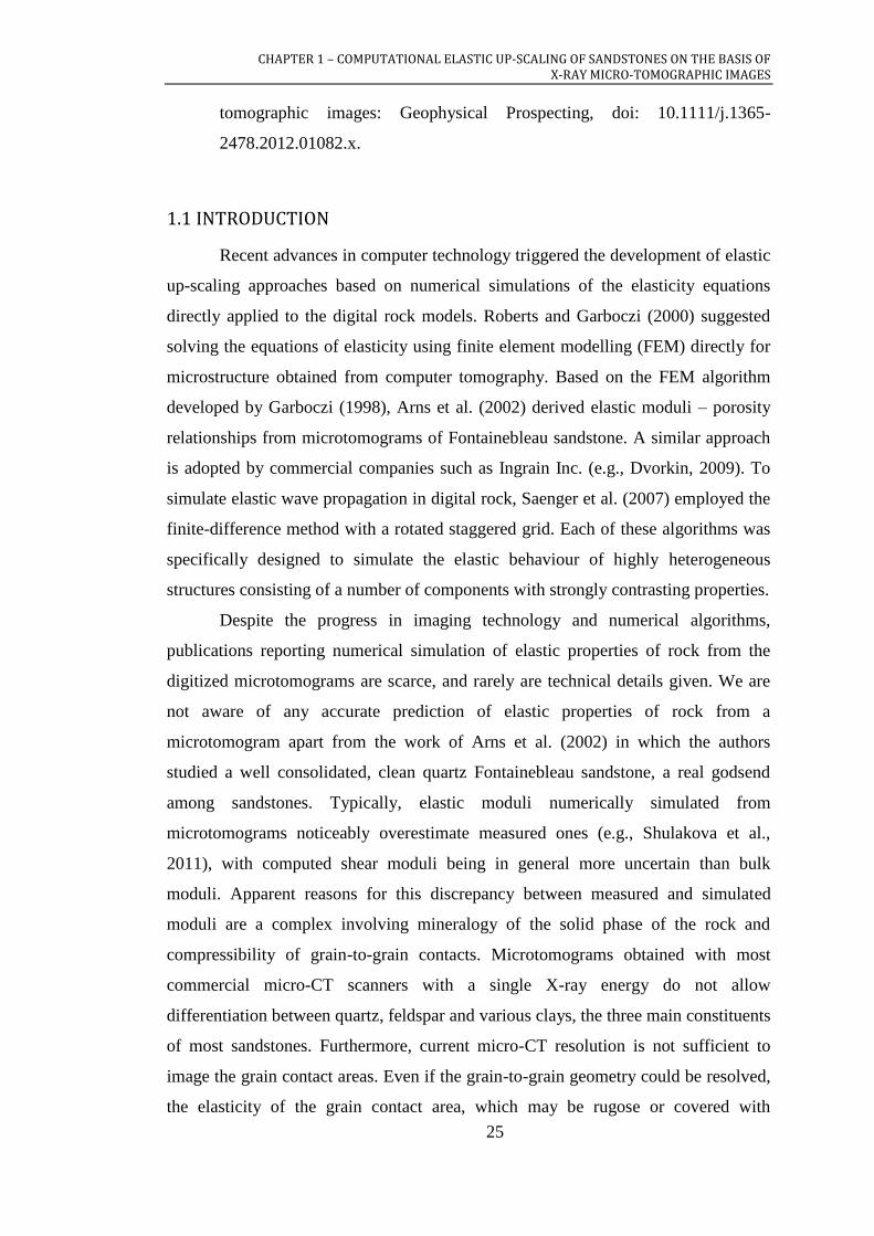
solid phase and a pore space. Then the original cube is subdivided into eight pieces
of 2003 pixels each (Figure 1.2).
Figure 1.2 Donnybrook sandstone microstructure: (a) reconstructed images in three perpendicular
directions, (b) interfacial surface: solid phase is transparent and pore space is shown by magenta. The
original cube of 400×400×400 pixels is subdivided into eight cubes of 2003 pixels as shown.
1.3 IMAGE PROCESSING AND MESHING
Micro-CT images cannot be directly used for numerical simulations; they
require pre-processing and segmentation into mineral and pore space phases. The
data initially come as a set of 2D images, which are later stacked together to form 3D
volume. Therefore, the processing of microtomograms can be either 2D slice-based
or 3D volume based. Calculations in 2D only are generally much faster than 3D
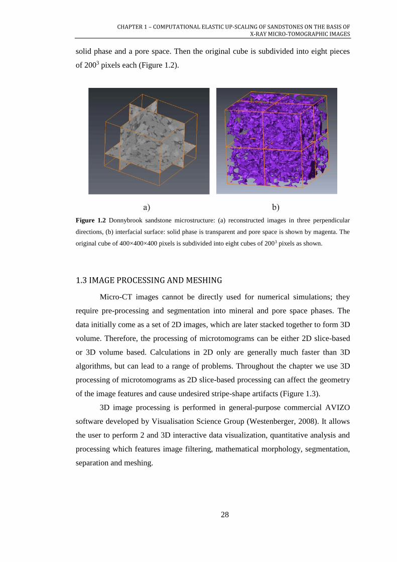
algorithms, but can lead to a range of problems. Throughout the chapter we use 3D
processing of microtomograms as 2D slice-based processing can affect the geometry
of the image features and cause undesired stripe-shape artifacts (Figure 1.3).
3D image processing is performed in general-purpose commercial AVIZO
software developed by Visualisation Science Group (Westenberger, 2008). It allows
the user to perform 2 and 3D interactive data visualization, quantitative analysis and
processing which features image filtering, mathematical morphology, segmentation,
separation and meshing.
CHAPTER 1 – COMPUTATIONAL ELASTIC UP-SCALING OF SANDSTONES ON THE BASIS OF X-RAY MICRO-TOMOGRAPHIC IMAGES
29
Figure 1.3 Effect of 2D routines (horizontal stripes) applied to the 3D sample of Donnybrook
sandstone.
1.3.1 IMAGE PRE-PROCESSING FOR NOISE SUPPRESSION
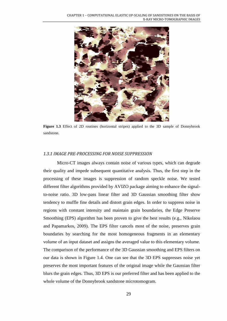
Micro-CT images always contain noise of various types, which can degrade
their quality and impede subsequent quantitative analysis. Thus, the first step in the
processing of these images is suppression of random speckle noise. We tested
different filter algorithms provided by AVIZO package aiming to enhance the signal-
to-noise ratio. 3D low-pass linear filter and 3D Gaussian smoothing filter show
tendency to muffle fine details and distort grain edges. In order to suppress noise in
regions with constant intensity and maintain grain boundaries, the Edge Preserve
Smoothing (EPS) algorithm has been proven to give the best results (e.g., Nikolaou
and Papamarkos, 2009). The EPS filter cancels most of the noise, preserves grain
boundaries by searching for the most homogeneous fragments in an elementary
volume of an input dataset and assigns the averaged value to this elementary volume.
The comparison of the performance of the 3D Gaussian smoothing and EPS filters on
our data is shown in Figure 1.4. One can see that the 3D EPS suppresses noise yet
preserves the most important features of the original image while the Gaussian filter
blurs the grain edges. Thus, 3D EPS is our preferred filter and has been applied to the
whole volume of the Donnybrook sandstone microtomogram.
CHAPTER 1 – COMPUTATIONAL ELASTIC UP-SCALING OF SANDSTONES ON THE BASIS OF X-RAY MICRO-TOMOGRAPHIC IMAGES
30
Figure 1.4 Comparison of different filters on the fragment of 3D Donnybrook sandstone: a) original
image, b) 3D Gaussian smoothing filter, and c) 3D edge preserve smoothing.
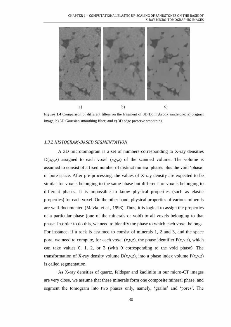
1.3.2 HISTOGRAM-BASED SEGMENTATION
A 3D microtomogram is a set of numbers corresponding to X-ray densities
D(x,y,z) assigned to each voxel (x,y,z) of the scanned volume. The volume is
assumed to consist of a fixed number of distinct mineral phases plus the void ‘phase’
or pore space. After pre-processing, the values of X-ray density are expected to be
similar for voxels belonging to the same phase but different for voxels belonging to
different phases. It is impossible to know physical properties (such as elastic
properties) for each voxel. On the other hand, physical properties of various minerals
are well-documented (Mavko et al., 1998). Thus, it is logical to assign the properties
of a particular phase (one of the minerals or void) to all voxels belonging to that
phase. In order to do this, we need to identify the phase to which each voxel belongs.
For instance, if a rock is assumed to consist of minerals 1, 2 and 3, and the space
pore, we need to compute, for each voxel (x,y,z), the phase identifier P(x,y,z), which
can take values 0, 1, 2, or 3 (with 0 corresponding to the void phase). The
transformation of X-ray density volume D(x,y,z), into a phase index volume P(x,y,z)
is called segmentation.
As X-ray densities of quartz, feldspar and kaolinite in our micro-CT images
are very close, we assume that these minerals form one composite mineral phase, and
segment the tomogram into two phases only, namely, ‘grains’ and ‘pores’. The

CHAPTER 1 – COMPUTATIONAL ELASTIC UP-SCALING OF SANDSTONES ON THE BASIS OF X-RAY MICRO-TOMOGRAPHIC IMAGES
31
mineral composition is taken into account at the later stage (see Section – 1.4
Numerical simulation of effective bulk and shear moduli).
The segmentation is based on a simple threshold (histogram-based)
algorithm, which assigns labels to voxels according to their intensities. While this
approach is considered to be adequate for this type of rock, we are aware that
segmentation based on voxel intensity alone will not work universally for all rock
types. The final segmentation of the Donnybrook sandstone is shown in Figure 1.5.
The white patches represent grains (blue segment on the histogram) and the black
patches are pores (white segment on the histogram). Suitable thresholds are found
from image histograms showing the number of occurrences of voxel values and the
current partitioning of the intensity range.
Histogram-based segmentation algorithms do not properly treat overlapping
distributions (e.g., Kaestner et al., 2008) and thus can lead to errors in phase
segmentation and phase fractions obtained from microtomograms. Later we analyse
the sensitivity of simulated elastic properties to variations in porosity arising from
the variation of histogram cut-off values. For this study we opted to treat the solid as
a single entity, and incorporate the effects of mineralogical variations through an
averaging procedure rather than retaining distinct phases for quartz, feldspar and clay
throughout the meshing and computation steps. The segmented tomogram could
therefore be converted into a binary format where pore and grain are presented by
zeros and ones, respectively. Further operations as described below are then needed
to arrive at effective properties of the homogenized solid.
Figure 1.5 A tomographic slice of a 3D image of a sandstone sample: a) original greyscale image, b)
its segmented image consists of two phases – matrix (white patterns) and pore space (black patterns),
c) image histogram showing the number of occurrences of voxel values and the current partitioning of
the intensity range.

CHAPTER 1 – COMPUTATIONAL ELASTIC UP-SCALING OF SANDSTONES ON THE BASIS OF X-RAY MICRO-TOMOGRAPHIC IMAGES
32
1.3.3 EFFECTIVE MEDIUM CALCULATION OF AVERAGED SOLID PROPERTIES
The micro-CT images of the Donnybrook sample do not have strong contrast
in X-ray density between quartz, feldspar and kaolinite, and hence do not allow
reliable discrimination between these minerals based on voxel intensity alone.
Instead, we estimate the bulk and shear moduli of the solid phase by means of the
effective medium theory, namely the self-consistent approximation (SCA)
(Berryman, 1980). This approximation was specifically designed to provide
estimates that are symmetric with respect to all constituents (that is, it does not treat
any constituent as a host or inclusion). Bulk and shear moduli are chosen as 39 and
33 GPa for quartz (Han et al., 1986), 76 and 26 GPa for plagioclase feldspar (Woeber
et al., 1963) and 12 and 6 GPa for kaolinite (Vanorio et al., 2003). Volumetric
fractions of quartz, feldspar and kaolinite are determined from 2-D SEM image
(Figure 1.1a) as 75%, 13% and 12%, respectively. Assuming (from SEM images,
Figure 1.1b) that the aspect ratio of the grains is about 1, we obtain effective bulk
and shear moduli of the solid phase as 37 GPa and 27 GPa, respectively. The
adequacy of these assumptions and our implementation of SCA procedures can only
really be tested by comparing computations (described next) against laboratory
measurements of the rock elastic properties.
1.3.4 MESH GENERATION AND SIMPLIFICATION
In order to perform finite-element simulation of physical properties, a finite
element mesh needs to be constructed. The two-phase segmented microtomogram is
then subjected to meshing. First, interphase surfaces are represented by a set of
triangles (so called triangular approximation). In AVIZO, this function is performed
by SurfaceGen routine. As this and following methods are time and resource
consuming, we have divided our 3-D volume into eight smaller subvolumes, and
perform all the processing separately for individual subvolumes. The triangulated
interface surfaces contain an enormous number of about 106 faces. Such a detailed
mesh is often unnecessary, and can be reduced by a given factor S using AVIZO’s
edge collapsing algorithm (Garland and Heckbert, 1997). Numerical tests show that
reduction of the mesh by a factor, S, up to 5 produces a geometrical configuration
very close to the original mesh. After the simplification, a so-called edge-flipping
CHAPTER 1 – COMPUTATIONAL ELASTIC UP-SCALING OF SANDSTONES ON THE BASIS OF X-RAY MICRO-TOMOGRAPHIC IMAGES
33
technique (De Berg et al., 2008) is applied to triangles that do not meet the Delaunay
criterion (Delaunay, 1934; Barber et al., 1996).
Using a reduction factor S > 5 for the simplification algorithm results in
oversimplified surfaces that do not preserve important details. To reduce the number
of surfaces further, we use re-meshing algorithms. The best isotropic (BI) and high
regularity (HR) re-meshing algorithms implemented in AVIZO allow us to keep fine
details by fixing profiles of surfaces. The best isotropic vertex placement algorithm is
based on Lloyd relaxation (Surazhsky et al., 2003). This high regularity algorithm
uses explicit regularization of the triangles around a vertex (Szymczak et al., 2003;
Alliez et al., 2005). While a decrease in a number of faces is crucially important for
speed-up, it also causes distortion in pore shape and perturbs the total porosity. To
estimate the effect of such distortion on resultant simulated elastic moduli, we tested
50%, 70% and 90% triangle number reduction for each algorithm. The described
workflow of a surface generation, simplification and re-meshing is applied to all the
real and model samples below. The only difference in the procedures is a re-meshing
algorithm and face reduction coefficients used in re-meshing. Hereafter, we name
meshes according to the name of the re-meshing algorithm used and the face
reduction coefficient. For instance, mesh HR90 means that the mesh is produced by
SurfaceGen routine followed by simplification and re-meshing with high regularity
algorithm employing 90% face reduction. The most relevant re-meshing procedure is
chosen below based on the comparison of numerical results with the exact theoretical
predictions.
1.4 NUMERICAL SIMULATION OF EFFECTIVE BULK AND SHEAR MODULI
1.4.1 ALGORITHM AND SOFTWARE
For numerical simulation of elastic moduli, we use the finite element method
that has been utilized in a number of works for elastic (and poroelastic) simulations.
The simulations are performed by means of ABAQUS FEA software – a suite of
software applications for finite element modelling, meshing and visualization –
developed by Dassault Systèmes (http://www.3ds.com). To simulate the uniaxial
deformation (P-wave) modulus M of a cubic volume, a normal displacement is
applied to one of the faces, say, to the top of the cube while on all other faces the

CHAPTER 1 – COMPUTATIONAL ELASTIC UP-SCALING OF SANDSTONES ON THE BASIS OF X-RAY MICRO-TOMOGRAPHIC IMAGES
34
normal the displacement is set to zero (Figure 1.6a). The modulus is then calculated
as the ratio of the average stress to average strain ,x xM where angle
brackets denote averaging over all the elements. To simulate the shear modulus µ, a
shear displacement is applied to the same face while the opposite face is fixed
(Figure 1.6b). The bulk modulus is then calculated from M and shear modulus µ as
3/4 MK . In this study, we assume the sample to be isotropic and, thus, the choice
of faces of loading and directions of displacement is not important.
Figure 1.6 Schematic model of displacements applied to the faces of the cube to calculate (a) P-wave
modulus and (b) shear modulus.
1.4.2 MESHING UNCERTAINTY
To analyse the effect of meshing on porosity and elastic properties, we have
tested it on the spherical inclusion model for which an exact analytical solution is
known. We create a 200×200×200 cubic model with a spherical cavity with radius of
25 units at the centre (Figure 1.7). A 3D volume is first generated by stacking a
series of 2D tiff images with the nearest-neighbour interpolation algorithm. After
assigning phase types as “solid” for the exterior and “pore” for the spherical
inclusion, the SurfaceGen algorithm is used to create a triangulated interface. This
interface contains 2.5·105 points and 5·105 faces. Then, this interface, is simplified
to 0.5·105 points and 1·105 faces. Remeshing is done with HR and BI algorithms
using 50%, 70% and 90% reduction coefficients. Any surface composed of triangles
is checked for the presence of triangle intersections, which are removed manually by
repositioning the corresponding tips. The results for both the algorithms look similar,
CHAPTER 1 – COMPUTATIONAL ELASTIC UP-SCALING OF SANDSTONES ON THE BASIS OF X-RAY MICRO-TOMOGRAPHIC IMAGES
35
though the BI algorithm tends to produce surfaces with fewer intersections. Finally,
the meshing of the phase volumes is generated using the TetraGen routine.
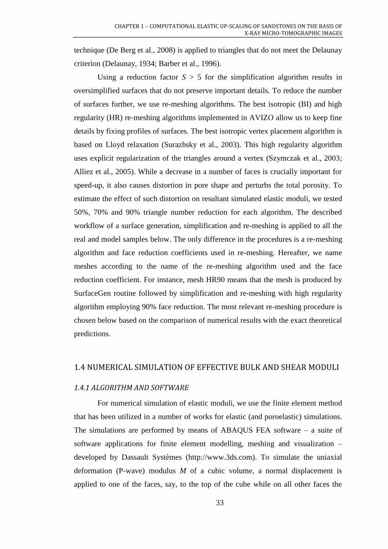
The six different models (BI50, BI70, BI90, HR50, HR70 and HR90) are
produced by applying different meshing algorithms (best isotropic and high
regularity) to this simple geometry with 50%, 70% and 90% of reduction (Figure
1.7c-f). Perturbation of porosity by meshing due to the discretization is shown in
Table 1.1. Even coarse meshing (BI90 and HR90) results in only subtle fluctuations
in porosity. However, even such small porosity perturbations along with possible
shape distortion due to discretization may affect the results of numerical simulations
of elastic properties. Below we compare results of numerical simulations of elastic
properties for all our models with known theoretical results.
Figure 1.7 Models used for FEM simulations: (a) geometry; (b) overlapped meshing of BI and HR
algorithms for spherical inclusion; (c) model BI70; (d) model BI50; (e) model HR70 and (f) model
HR50.

CHAPTER 1 – COMPUTATIONAL ELASTIC UP-SCALING OF SANDSTONES ON THE BASIS OF X-RAY MICRO-TOMOGRAPHIC IMAGES
36
Table 1.1 Model of spherical inclusion: surface re-meshing and volumetric gridding parameters.
Initial parameters: 25.16·104 points, 50.32·104 faces; simplified surface: 5.00·104 points, 10.00·104
faces.
Remeshing
algorithm
# points,
*104
# faces,
*104
# nodes,
*105
# triangles,
*106
# tetrahedrons,
*106
Porosity,
*10-3
Porosity
perturbation,%
BI
(%)
90 0.50 0.99 2.63 2.86 1.40 8.02 1.97
70 1.50 3.00 1.28 1.43 7.09 8.07 1.36
50 2.50 5.00 2.73 3.10 1.54 8.17 0.14
HR
(%)
90 0.50 1.00 2.65 2.89 1.42 8.02 1.97
70 1.53 3.0 1.30 1.47 7.27 8.07 1.36
50 2.56 5.13 2.81 3.20 1.59 8.10 0.99
1.4.3 NUMERICAL SIMULATION AND ACCURACY TESTING
We perform FEM simulations for a single spherical dry cavity with volume
3)3/4( Rp and a hydrostatic stress d applied at the infinity. The effective bulk
modulus effK for such a configuration is (Mavko et al., 1998):
KKK geff
11
. (1.1)
Here gK is bulk modulus of the mineral material and the single pore stiffness K is:
212
1311
gKK, (1.2)
where is the Poisson ratio of the mineral material.
The simulations are performed for two materials with highly contrasting
properties for the host material and spherical cavity. The bulk moduli are assumed to
be 35 and 10-5 GPa, respectively, and Poisson ratio of the spherical cavity is assumed
to be 0.5. Simulations are done for different Poisson ratios of 0.1, 0.16, 0.2, 0.3 and
0.4 of the host material. The results of the simulations are shown in Figure 1.8 for
both HR and BI algorithms with different reduction coefficients. The larger the value
Poisson ratio used, the larger is the deviation of the numerical solution from the
theoretical one. However, for all the values of , the numerical results converge to
the theoretical solution as the meshing quality is improved.
CHAPTER 1 – COMPUTATIONAL ELASTIC UP-SCALING OF SANDSTONES ON THE BASIS OF X-RAY MICRO-TOMOGRAPHIC IMAGES
37
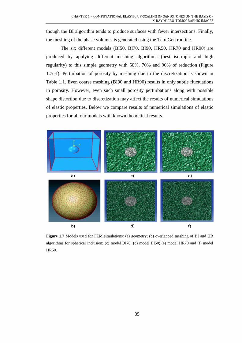
Figure 1.8 Comparison of the results of finite-element simulations with theoretical predictions for
meshing fulfilled in (a) AVIZO using the BI method; (b) AVIZO using the HR method.
To estimate the uncertainty caused by the finite size of mesh elements for
both HR and BI meshing algorithm with 50%, 70% and 90% of simplification, we
calculated relative error in simulated bulk modulus TKK , where K is an
absolute difference between numerically simulated and theoretically predicted bulk
modulus (TK ). Figure 1.9 shows the relative error of the bulk modulus against
porosity perturbation, for the two meshing algorithms. For BI meshing, K
linearly decreases with with proportionality coefficients of 2 and 3 for Poisson
ratios of 0.1 and 0.2, respectively, and tends to zero when the porosity perturbation
tends to zero. The proportionality constant between K and has values of 2 and
3 for Poisson ratios of 0.1 and 0.2, respectively. For the HR algorithm K shows
linear trends with as well but with twice the coefficients for the same Poisson
ratio.

CHAPTER 1 – COMPUTATIONAL ELASTIC UP-SCALING OF SANDSTONES ON THE BASIS OF X-RAY MICRO-TOMOGRAPHIC IMAGES
38
(a) (b)
Figure 1.9 Relative error of bulk modulus simulation caused by a finite size of a mesh element
against porosity uncertainty for the (a) high-regularity method of meshing in AVIZO and (b) best
isotropic method in AVIZO.
We prefer to use the BI algorithm for meshing the microstructure of the real
sample as (1.1) the relative error in bulk modulus TKK is smaller for the same
porosity perturbation and (1.2) the BI algorithm is more stable when processing large
volumes and complex geometry of real samples. The above analysis also allows
estimating an error of simulated elastic moduli caused by discrete meshing. Meshing
of the spherical inclusion model using BI50 and BI70 procedures causes relative
perturbation in porosity of 0.1% and 1%, respectively. Assuming that the same
meshing procedures lead to the same porosity perturbations in the case of the
sandstone sample with total porosity of about 15%, the porosity error caused by the
meshing is expected to be about 0.1- 1%. Using the relationship between errors in the
porosity and elastic moduli for the case of spherical cavity (Figure 1.9), we expect
that the uncertainty in elastic moduli caused by meshing will not exceed 1%.
1.4.4 MESHING AND NUMERICAL SIMULATION OF ELASTIC MODULI OF
DONNYBROOK SANDSTONE
The cube of 4003 voxels is cropped into eight cubic subvolumes of 2003
voxels as shown in Figure 1.2b. To estimate the scatter of the properties within this
sample, the porosity of subvolumes is calculated from segmented microtomograms
and shows the spread from 12% to 22%. Note that the sample does not have gross
heterogeneities or internal structures visible to the naked eye, so we can consider this
level property variation to be inherent in this type of natural sandstone.

CHAPTER 1 – COMPUTATIONAL ELASTIC UP-SCALING OF SANDSTONES ON THE BASIS OF X-RAY MICRO-TOMOGRAPHIC IMAGES
39
Each of these smaller cubes has been simplified and re-meshed using with the
BI algorithm with 50% of surface simplification.
Figure 1.10 illustrates different stages of surface evolution for the first
subvolume of the Donnybrook sample starting from (a) the original surface with
1,269,824 faces, followed by (b) simplification to 199,963 faces using edge-
collapsing algorithm and (c) reduction to 1,014,965 faces after the best isotropic re-
meshing algorithm reduced the surface by 50% from original.
Figure 1.10 Different stages of surface simplification for part 1 of Donnybrook sandstone sample: a)
original surface – 1,269,824 faces, b) simplified surface (edge collapsing algorithm) – 199,963 faces,
c) re-meshed surface (BI algorithm, reduced by 50%) – 1,014,965 faces.
Surface generation, simplification and re-meshing are followed by meshing
of the phase volumes by generating volumetric tetrahedral grids using the TetraGen
routine based on the advancing front method (AFM) (Yasushi et al., 2004). A mesh
of each of the eight subvolumes contains from 1.5-2.1 · 105 tetrahedra depending on
the remeshing procedure (see Table 1.2 for details).
Table 1.2 Donnybrook sandstone: volumetric grid and porosity parameters for all 8 parts.
Parts
1 2 3 4 5 6 7 8
φ 0.14 0.17 0.22 0.15 0.15 0.12 0.13 0.12
∆φ, % 0.97 1.18 0.67 1.26 1.28 1.65 2.03 1.56
Points, *104 4.9 4.9 5.0 4.9 4.6 5.6 4.4 4.9
Faces, *105 1.0 1.0 1.0 1.0 1.0 1.2 0.9 1.0
Nodes, *105 3.3 2.8 2.9 2.9 2.8 3.6 2.6 3.2
Triangles, *106 3.7 3.2 3.4 3.3 3.2 4.1 3.0 3.7
Tetraherda, *106 1.9 1.6 1.7 1.7 1.6 2.1 1.5 1.8
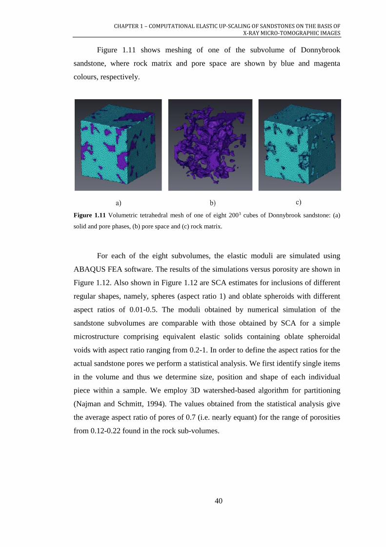
CHAPTER 1 – COMPUTATIONAL ELASTIC UP-SCALING OF SANDSTONES ON THE BASIS OF X-RAY MICRO-TOMOGRAPHIC IMAGES
40
Figure 1.11 shows meshing of one of the subvolume of Donnybrook
sandstone, where rock matrix and pore space are shown by blue and magenta
colours, respectively.
Figure 1.11 Volumetric tetrahedral mesh of one of eight 2003 cubes of Donnybrook sandstone: (a)
solid and pore phases, (b) pore space and (c) rock matrix.
For each of the eight subvolumes, the elastic moduli are simulated using
ABAQUS FEA software. The results of the simulations versus porosity are shown in
Figure 1.12. Also shown in Figure 1.12 are SCA estimates for inclusions of different
regular shapes, namely, spheres (aspect ratio 1) and oblate spheroids with different
aspect ratios of 0.01-0.5. The moduli obtained by numerical simulation of the
sandstone subvolumes are comparable with those obtained by SCA for a simple
microstructure comprising equivalent elastic solids containing oblate spheroidal
voids with aspect ratio ranging from 0.2-1. In order to define the aspect ratios for the
actual sandstone pores we perform a statistical analysis. We first identify single items
in the volume and thus we determine size, position and shape of each individual
piece within a sample. We employ 3D watershed-based algorithm for partitioning
(Najman and Schmitt, 1994). The values obtained from the statistical analysis give
the average aspect ratio of pores of 0.7 (i.e. nearly equant) for the range of porosities
from 0.12-0.22 found in the rock sub-volumes.

CHAPTER 1 – COMPUTATIONAL ELASTIC UP-SCALING OF SANDSTONES ON THE BASIS OF X-RAY MICRO-TOMOGRAPHIC IMAGES
41
Figure 1.12 Bulk and shear moduli simulated for all parts (circles) in comparison with SCA method
predictions for pores of different shapes from spheres (solid line) to oblate spheroids with aspect ratios
(0.01-0.5) (dashed lines).
1.4.5 COMPARISON WITH EXPERIMENTAL DATA
The numerically simulated bulk and shear moduli are shown in Figure 1.13 in
comparison with experimental data obtained for Donnybrook sandstone at effective
stresses of 15-70 MPa using a pulse-transmission system operating at ultrasonic
frequencies. The experiment was first performed on a sample with a diameter of
38.15 mm and a length of 93.04 mm and then was repeated for a smaller sample with
the same diameter but a shorter length of 56 mm. The experimental data are shown
by solid circles with error bars corresponding to measurement uncertainty. The
results of numerical simulations are shown by lines parallel to the effective stress
axis as the elastic moduli obtained. Note that the porosity of the sample employed for
ultrasonic measurements is 15% and the simulated moduli are shown for the
subvolume with the same porosity taken from among the 8 smaller cubes. Linear
trends that characterize elastic moduli variations at high pressures of 50-70 MPa are
shown by dashed lines.
One can see that numerically simulated moduli correspond to the
measurements at the confining stress of about 40-50 MPa. To explain the differences
between the simulated and experimentally measured moduli, we consider three
different effective stress ranges, namely, low effective stresses 0-50 MPa,
intermediate stresses of about 50 MPa and high effective stresses of 50-70 MPa. At
low effective stresses, the elastic moduli are strongly affected by compliant porosity

CHAPTER 1 – COMPUTATIONAL ELASTIC UP-SCALING OF SANDSTONES ON THE BASIS OF X-RAY MICRO-TOMOGRAPHIC IMAGES
42
represented by grain contacts and microcracks. Such microcracks reduce elastic
moduli dramatically at low stresses (e.g., Shapiro, 2003; Angus et al., 2009;
MacBeth, 2004; Liu H. H. et al., 2006). However, these microcracks are too thin and
have too small aspect ratios (10-4 to 10-3) to be detected by X-ray microtomography
(even though it is performed at ambient pressure), and therefore are not accounted
for in numerical simulations. Indeed, the larger part of each grain-to-grain contact in
a microtomogram (Figure 1.1a) is likely to be a highly compliant void of a low
aspect ratio (see Figure 1.1b), but is treated in our processing as a welded contact.
Thus simulated elastic moduli represent the sample without compliant porosity, and
correspond to measurements at such pressures where such compliant porosity is
effectively closed with respect to transmission of shear and normal tractions. The
closure of compliant porosity results in exponential dependency of the moduli with
effective confining pressure (e.g., Shapiro, 2003; Ciz and Shapiro, 2009; Pervukhina
et al., 2010) and further discussed in Chapter 3.
Figure 1.13 shows this exponential dependency in the experimental data up to
the pressure of about 50 MPa. This is precisely where the measurements and
simulations agree. At higher stresses of 50-70 MPa, we observe in the experimental
points a linear trend of elastic moduli with pressure. Linear dependency of elastic
moduli on stress at stresses above 40-50 MPa are a common feature of many rocks
(Eberhard-Phillips et al., 1989), and is usually attributed to a decrease of stiff
porosity (Mavko and Jizba, 1991; Shapiro, 2003; Vernik and Kachanov, 2010). The
numerical simulations do not take into account this reduction of porosity (as the
microtomograms are obtained at zero stress) and, thus, underestimate the
experimentally measured elastic moduli.
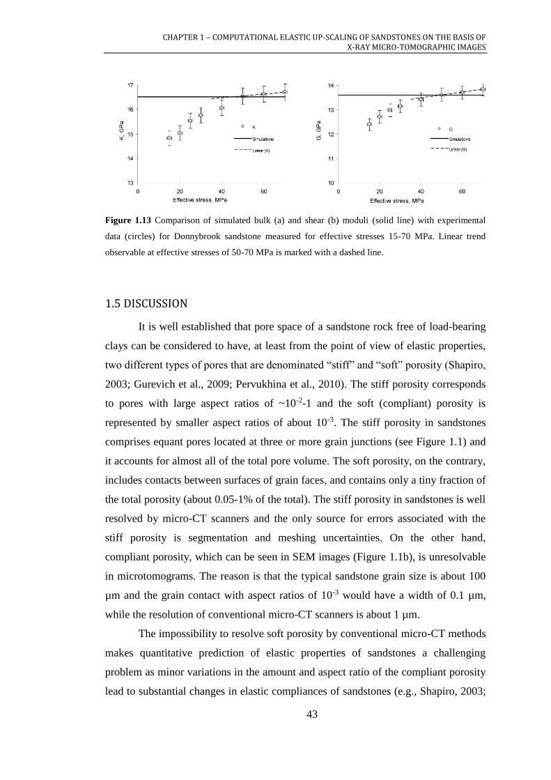
CHAPTER 1 – COMPUTATIONAL ELASTIC UP-SCALING OF SANDSTONES ON THE BASIS OF X-RAY MICRO-TOMOGRAPHIC IMAGES
43
Figure 1.13 Comparison of simulated bulk (a) and shear (b) moduli (solid line) with experimental
data (circles) for Donnybrook sandstone measured for effective stresses 15-70 MPa. Linear trend
observable at effective stresses of 50-70 MPa is marked with a dashed line.
1.5 DISCUSSION
It is well established that pore space of a sandstone rock free of load-bearing
clays can be considered to have, at least from the point of view of elastic properties,
two different types of pores that are denominated “stiff” and “soft” porosity (Shapiro,
2003; Gurevich et al., 2009; Pervukhina et al., 2010). The stiff porosity corresponds
to pores with large aspect ratios of ~10-2-1 and the soft (compliant) porosity is
represented by smaller aspect ratios of about 10-3. The stiff porosity in sandstones
comprises equant pores located at three or more grain junctions (see Figure 1.1) and
it accounts for almost all of the total pore volume. The soft porosity, on the contrary,
includes contacts between surfaces of grain faces, and contains only a tiny fraction of
the total porosity (about 0.05-1% of the total). The stiff porosity in sandstones is well
resolved by micro-CT scanners and the only source for errors associated with the
stiff porosity is segmentation and meshing uncertainties. On the other hand,
compliant porosity, which can be seen in SEM images (Figure 1.1b), is unresolvable
in microtomograms. The reason is that the typical sandstone grain size is about 100
µm and the grain contact with aspect ratios of 10-3 would have a width of 0.1 µm,
while the resolution of conventional micro-CT scanners is about 1 µm.
The impossibility to resolve soft porosity by conventional micro-CT methods
makes quantitative prediction of elastic properties of sandstones a challenging
problem as minor variations in the amount and aspect ratio of the compliant porosity
lead to substantial changes in elastic compliances of sandstones (e.g., Shapiro, 2003;
CHAPTER 1 – COMPUTATIONAL ELASTIC UP-SCALING OF SANDSTONES ON THE BASIS OF X-RAY MICRO-TOMOGRAPHIC IMAGES
44
Pervukhina et al., 2010). However micro-CT images contain all the necessary
information to obtain moduli at high effective stresses as all existing theories accept
that soft porosity shows exponential decay with an increase of effective stress and
vanishes at stresses higher than 50-60 MPa (e.g., Pervukhina et al., 2010; Shapiro,
2003; Becker et al., 2007). Additionally, the images include information of probable
sources of soft porosity at grain contacts, namely, their surface areas and orientation
angles.
Soft porosity evaluated from fitting of stress dependency of experimentally
measured compressibility (a reciprocal of bulk moduli) of dry rock by method
suggested by Pervukhina et al. (2010) is shown in Figure 1.14a. An additional
independent proof of the presence of soft porosity at low effective stresses and its
closure at higher stresses can be given comparing the experimental moduli measured
on the saturated sample with moduli calculated using Gassmann fluid substitution
(Gassmann, 1951) obtained from experimentally measured dry moduli (Figure
1.14b). Measured and Gassmann-computed saturated moduli are in a good agreement
at high stresses, but show obvious divergence at lower effective stresses. This
discrepancy between the moduli at low stresses can be explained by squirt effect
(viscous dampening when water fills the cracks) that implies the presence of
compliant porosity (Mavko and Jizba, 1991; Gurevich et al., 2009). With increase of
effective stress and closure of soft porosity, the squirt effect vanishes and the
difference of between the measured bulk moduli and that estimated by Gassmann
substitution becomes negligible (within the experimental error).
The procedure developed for image processing, interfacial surface
triangulation and simplification, meshing and numerical simulation of elastic
properties of rocks can be applied without much change for the analysis of 3D rock
microstructure data obtained by Scanning Electron Microscope (SEM) combined
with Focused Ion Beam (FIB) technology (e.g., Drury and Fitz Gerald, 1996;
Matthijs de Winter et al., 2009) or other emerging techniques that increase the
resolution down to nanometre scale. By employing such high-resolution techniques,
numerical prediction of elastic properties might be possible at different confining
stresses even with complex particle contacts. Further improvements can also come
from the application of multi-energy data acquisition and processing (e.g.,
Shikhaliev, 2008; Yang et al., 2010; Qi et al., 2010) which allows clear

CHAPTER 1 – COMPUTATIONAL ELASTIC UP-SCALING OF SANDSTONES ON THE BASIS OF X-RAY MICRO-TOMOGRAPHIC IMAGES
45
differentiation between grains with different mineralogy that would otherwise be
lumped into a single “phase” in a single-energy tomogram. The segmentation of solid
phase into the true mineral distribution then becomes possible and different elastic
moduli can be attributed explicitly to individual grains instead of the use of the SCA
to calculate effective elastic moduli of and averaged solid phase.
(a) (b)
Figure 1.14 Illustration of existence of soft porosity in Donnybrook sandstone: (a) soft porosity
calculated from stress dependency of bulk modulus shows exponential decay and almost vanishes at
50 MPa; (b) Experimentally measured saturated bulk moduli in comparison with bulk moduli
calculated using Gassmann fluid substitution equation from dry moduli at different effective stresses.
Two saturated moduli show obvious difference at low effective stresses and are in a good agreement
at higher stresses.
It is also noteworthy that our computational approach can be readily extended
in various directions. The algorithms already used can be scaled up to allow for much
larger simulation sizes, given sufficient computational power (e.g., GPU cluster),
allowing larger rock volumes and/or higher resolution datasets to be tackled. We
have not fully explored the capabilities of available adaptive grids algorithms. This
becomes a crucial step if the modelling domain increases or other fields are
simultaneously computed. For example, effective poroelastic rock behaviour of fluid-
saturated rocks are of interest but require finer meshing in order to resolve fluid
pressure diffusion processes (e.g., Wenzlau and Müller, 2009; Wenzlau et al., 2010).
With adaptive meshing this complexity can be included without change in the overall
numerical setup.

CHAPTER 1 – COMPUTATIONAL ELASTIC UP-SCALING OF SANDSTONES ON THE BASIS OF X-RAY MICRO-TOMOGRAPHIC IMAGES
46
1.6 CHAPTER CONCLUSIONS
We have developed a comprehensive digital rock physics workflow including
3D imaging, processing and finite-element simulations of physical experiments with
the focus on the numerical up-scaling of elastic moduli. As an example, the effective
elastic bulk and shear moduli of a Donnybrook sandstone sample are numerically
simulated using microtomograms. The simulated and measured elastic moduli are in
a good agreement at the effective stress of about 50 MPa, which is the stress level
where microcracks become effectively closed. We conclude that the computational
elastic up-scaling approach yields physically consistent effective moduli for this rock
microstructure, which is typical of many consolidated reservoir sandstones and
aquifers. The grains are mainly quartz and feldspars with some clay and a moderate
porosity and permeability is exhibited. To account for sub-resolution features, either
theoretical or additional computational approaches need to be employed. Further
research along these lines is also required to account for the full range of frequency
and stress-dependent behaviour observed.

CHAPTER 2 – EXPERIMENTAL VERIFICATION OF THE PHYSICAL NATURE OF VELOCITY-STRESS RELATIONSHIP FOR ISOTROPIC POROUS ROCKS
47
CHAPTER 2 – EXPERIMENTAL VERIFICATION OF THE PHYSICAL NATURE OF VELOCITY-STRESS RELATIONSHIP FOR ISOTROPIC POROUS ROCKS
The exponential increase of seismic velocities with effective stress has
usually been explained by the presence of pores with a broad distribution of aspect
ratios. More recently, a stress-related closure of soft pores with a narrow distribution
of compliances (e.g., grain contacts) has been suggested to be sufficient to explain
such exponential stress dependency. Here we verify this theoretical interpretation
using laboratory measurements on dry sandstones. Based on the experimental data,
linear dependency of elastic compressibility on soft porosity and exponential decay
of soft porosity and elastic compressibility with effective stress up to 60 MPa is
confirmed. Soft porosity, estimated from the fitting coefficients of elastic
compressibilities, is on the same order of magnitude but slightly lower than obtained
from strain measurements. The results confirm applicability of previously proposed
stress sensitivity models and provide justification for using this approach to model
stress dependency of elastic properties for isotropic and anisotropic rocks.
In this chapter, I used the material published in the following extended
abstract with permission from leading co-authors:
Pervukhina M., Gurevich B., Dewhurst D. N., Siggins A. F., Golodoniuc P.,
and Fortin J., 2010, Experimental verification of the physical nature of
velocity-stress relationship for isotropic porous rocks: ASEG Extended
Abstract at the 21st International Geophysical Conference and Exhibition
(ASEG-PESA), Sydney, Australia.
2.1 INTRODUCTION
Knowledge of stress dependency of elastic properties of rocks is important
for a variety of geophysical applications ranging from pore pressure prediction in
sedimentary rocks and seismic monitoring of hydrocarbon production to constraining
material properties in the mantle. It has been shown by many authors that stress
dependency of compressional and shear velocity V in many dry porous rocks can be
well approximated by a combination of linear and exponential terms (e.g.,
Zimmerman et al., 1991; Eberhart-Phillips et al., 1989):

CHAPTER 2 – EXPERIMENTAL VERIFICATION OF THE PHYSICAL NATURE OF VELOCITY-STRESS RELATIONSHIP FOR ISOTROPIC POROUS ROCKS
48
)exp()( PDBKPAPV , (2.1)
where P is confining pressure, A, K, B, and D are fitting parameters that provide the
best agreement with the measured data.
The exponential term in equation (2.1) is usually explained by presence of
pores and cracks with a broad (often exponential) distribution of crack stiffnesses or
aspect ratios. An attempt to explain the nonlinearity with cracks of similar shape was
done by Mavko and Nur (1978) and resulted in polynomial strain vs. stress
dependency and specific shape of non-elliptical cracks. Recently, Shapiro (2003)
obtained a result that such exponential saturated to linear form may be explained by
much more simple and physically plausible dual distribution of porosity. More
precisely, Shapiro (2003) showed that if total porosity of an isotropic rock can be
divided into stiff porosity part s and much more compliant part c , i.e.:
s c (2.2)
then dry rock compressibility drC can be written as a simple linear function of stiff
and compliant porosities:
1dr drs s s c cC P C
(2.3)
Here drsC is the compressibility of the porous rock with all compliant
porosity closed (hereafter, stiff limit), s and c s are coefficients related to
compliance of stiff and compliant pores, respectively, 0s s s is the deviation
of the stiff porosity from its zero-pressure value 0s . Compliant porosity c and
s are assumed as low as 10% or less (Shapiro, 2003) to satisfy the assumption of
linear variation of compressibility with porosity and independent in a sense that
closure of c does not affect s and vice versa. Note a change in notation: s in
the present work corresponds to s in Shapiro (2003).
In many cases, s s c c and equation (2.3) reduces to:
1dr drs c cC P C
(2.4)

CHAPTER 2 – EXPERIMENTAL VERIFICATION OF THE PHYSICAL NATURE OF VELOCITY-STRESS RELATIONSHIP FOR ISOTROPIC POROUS ROCKS
49
Variations of stiff and soft porosity with pressure have the form:
01s gr s drsP C C (2.5)
and
0 expc c c drsC P
(2.6)
where grC is the compressibility of the solid grain material and 0c is the compliant
porosity at zero pressure. Equation (2.5) is slightly more general than the form used
by Shapiro (2003), as it does not require initial stiff porosity 0s to be small.
Substituting expression (2.6) for compliant porosity into equation (2.4) gives the
variation of compressibility with pressure dr dr drsC P C P C in the form:
PCCPC drscccdrsdr exp0 (2.7)
If this variation is small ( drsdr CPC ), then equation (2.3) together with
the corresponding equation for the shear compliance yields equations similar in form
to (2.1) for the bulk and shear moduli and for compressional and shear velocities of
the dry rock (Shapiro, 2003). The moduli and velocities of saturated rocks (at low
frequencies) can be obtained using Gassmann equations; in this case pressure P has
the meaning of effective pressure.
The stress sensitivity theory of Shapiro (2003) was extended to anisotropic
rocks by Shapiro and Kaselow (2005). A number of studies use the theory to describe
behaviour of various isotropic and anisotropic rocks, for instance, Becker et al.,
(2007), Pervukhina et al. (2008a), Pervukhina et al. (2008b), Liu et al. (2008) and De
Paula et al. (2008).
While the stress sensitivity approach of Shapiro (2003) provides an
appealingly simple interpretation of equation (2.1) and the existence of compliant
porosity has been reported by many authors, it is not yet widely accepted, partly due
to the lack of the experimental verifications of this interpretation. The main difficulty
in such experimental verification lies in the fact that, in most cases, the velocity-
stress relationship is obtained through ultrasonic experiments where variation of
porosity with stress is not simultaneously measured.

CHAPTER 2 – EXPERIMENTAL VERIFICATION OF THE PHYSICAL NATURE OF VELOCITY-STRESS RELATIONSHIP FOR ISOTROPIC POROUS ROCKS
50
In this chapter, we overcome this difficulty by using simultaneous
measurements of ultrasonic velocity and porosity in a high-pressure cell. Porosity
variations are estimated from measurements of axial strain. The results of our
analysis for the sandstone samples used in the experiments are consistent with the
physical interpretation of Shapiro (2003).
2.2 WORKFLOW
Our workflow consists of three main parts: laboratory measurements,
computation of the key parameters, and analysis.
2.2.1 EXPERIMENT
The experimental program involves the following steps:
1. Measure compressional Vp and shear Vs velocities for a dry sample as a
function of isotropic confining pressure P.
2. Simultaneously measure axial strain ax as a function of pressure.
3. Measure initial porosity at zero pressure 0 and/or initial density 0 .
2.2.2 CALCULATIONS OF KEY PARAMETERS
Once these data are measured, compressibilities plus stiff and soft porosities
are obtained as follows:
1. For each pressure, the dry bulk modulus drK is obtained using the standard
equation 2 2
04 3dr P SK V V and compressibility as 1
dr drC K . Note that
accuracy of the calculation of the bulk modulus using initial density 0 at
0P should be checked for a particular rock since the introduced error
might be sufficient for a compliant rock. In the case of our samples, we have
estimated density perturbations from axial strain measurements assuming that
CHAPTER 2 – EXPERIMENTAL VERIFICATION OF THE PHYSICAL NATURE OF VELOCITY-STRESS RELATIONSHIP FOR ISOTROPIC POROUS ROCKS
51
all deformations are isotropic and found that the error caused by use of the
initial density 0 is less than 0.4%.
2. We then compute variation of porosity with pressure. Since experiments are
performed with hydrostatic pressure, we assume that ax represents the strain
in all three directions. Then, the volumetric strain (relative variation of the
sample volume v with pressure) is 0 0( ) / 3 axv v v , where 0v is
sample volume at zero pressure. At the same time, the relative change of total
volume grv of solid grains with pressure is
0 0( ) / / 1gr gr gr gr grv v v C P , where 0grv is total volume of solid
grains at zero pressure and grC is the compressibility of the solid grain
material, which is assumed known from mineralogical analysis. Since pore
volume at any pressure is the total volume minus grain volume, grv v v ,
using Zimmerman et al. (1986), we get:
0
0
1 / 11 1
1
gr grgrC P vvv
v v v
(2.8)
For small deformations, this gives:
0 0 01 1 1 1gr grC P C P
(2.9)
Note that for 0P , total volumetric strain, , is negative, and is larger in
absolute value than the grain deformation grC P ; therefore, using (2.9),
porosity will decrease with increasing pressure, as it should.
3. Now we have to define the parameters, which we called stiff and soft
porosities. Since stiffness of pores is a relative measure, there is some
freedom inherent in this distinction. One way to define stiff porosity is to
assume that within the pressure range of measurements, say from 0-100 MPa,
the stiff porosity changes linearly with pressure. Indeed, if measured
CHAPTER 2 – EXPERIMENTAL VERIFICATION OF THE PHYSICAL NATURE OF VELOCITY-STRESS RELATIONSHIP FOR ISOTROPIC POROUS ROCKS
52
compressibilities and velocities can be described by a simple exponential
relationship of the type given by equation (2.4), then at large pressures the
compressibility drC approaches a constant value drsC . Constant
compressibility corresponds to a linear variation of the strain with pressure.
Indeed, in a pressure interval where dry compressibility is approximately
constant, dr drsC C , volumetric strain
drC P and equation (2.8) gives a
linear relationship between porosity and pressure. This linear porosity trend is
expected in the upper part of our pressure range, where all soft pores can be
assumed closed. We can thus call this part of the porosity the stiff porosity.
Assuming, following Shapiro (2003), that stiff and soft porosity variations are
independent of one another, we can extrapolate this stiff porosity trend to
lower pressures. In practice, we will estimate stiff porosity by fitting a linear
trend to the porosity-pressure dependency in the uppermost part of the
measurement pressure range (Walsh, 1965; Mavko and Jizba, 1991).
4. Once stiff porosity is defined, the compliant (soft) porosity is defined by
equation (2.2) as the difference between total and stiff porosity. We will also
obtain soft porosity from a non-linear fitting of experimentally measured
drC P as a ratio of the coefficient before the exponential to the exponent as
predicted by equation (2.7). Hereafter, we refer to the former and latter soft
porosity as measured and predicted, respectively.
We fitted experimentally measured compressibilities
PCCCPC drscccdrsdrsdr exp0 to get the best fit values of the stiff limit
drsC and then calculated dr dr drsC P C P C .
2.2.3 TESTING THEORETICAL PREDICTIONS
With equations (2.2) and (2.5) used effectively as definitions, we will test
experimentally the following elements of Shapiro’s (2003) stress sensitivity theory:
1. Test the adequacy of the linear relationship (2.4) between the dry compliance
and soft porosity.

CHAPTER 2 – EXPERIMENTAL VERIFICATION OF THE PHYSICAL NATURE OF VELOCITY-STRESS RELATIONSHIP FOR ISOTROPIC POROUS ROCKS
53
2. Test the adequacy of the exponential approximation, equation (2.6), for the
soft porosity.
3. Compare the exponent drscC in the soft porosity fit, equation (2.6), with the
same exponent in the drC fit, equation (2.7), hereafter, and C ,
respectively.
4. Compare the measured against predicted soft porosity.
5. Compare the two stress sensitivity coefficients appearing in equation (2.7).
The coefficient dyn obtained from the proportionality constant is called
dynamic because it is derived from the measurements of ultrasonic velocities.
In contrast, the coefficient in the exponent st, which describes variation of
soft porosity with pressure, is called static. In deriving these values from the
corresponding fits (linear fit of drC versus c and exponential fit for
drC
versus pressure) we assume that high-stress compressibility drsC is the same
in both instances.
2.3 DATA
We used reservoir sandstone core samples from the Northwest Shelf of
Australia between depths of 1700-2000 metres (Siggins and Dewhurst, 2003) to
validate the stress dependency model. The other sample we used in our research is a
cylindrical specimen of 80 mm in length and 40 mm in diameter that was prepared
from Bleurswiller Sandstone, which was collected from a quarry in Frain (Vosges,
eastern France). The experimental procedure and results were published in Fortin et
al. (2007). We calculate elastic compressibilities using longitudinal and shear
velocities in the dry samples. Porosity variations are obtained from changes in the
length of the cylindrical samples.
Total, stiff and compliant porosity are shown in Figure 2.1 for the
Bleurswiller Sandstone sample for loading phase. As outlined above, stiff porosity
(solid line) is obtained by linear extrapolation of the high-stress trend determined
from two points at 60 and 65 MPa. Compliant porosity (open circles) is estimated by
subtracting stiff porosity from the total porosity and is reasonably approximated by
an exponential fit (dashed line). The total porosity is shown as solid circles.

CHAPTER 2 – EXPERIMENTAL VERIFICATION OF THE PHYSICAL NATURE OF VELOCITY-STRESS RELATIONSHIP FOR ISOTROPIC POROUS ROCKS
54
Figure 2.1 Total, stiff and compliant porosities.
2.4 RESULTS
In Figures 2.2 and 2.3, we illustrate tests of the stress sensitivity theory for
the Bleurswiller sandstone and then show test results on all samples (Figure 2.4). The
test of linearity of the relationship between compressibility and soft porosity
(equation 2.4) is demonstrated in Figure 2.2, which shows pressure variation of
compressibility drC P as a function of compliant porosity and its linear fit for the
loading limb. The square of the Pearson product moment correlation coefficients R2
is 0.99 indicating a very good correlation between drC P and Pc .
Measured stress dependencies of variations of elastic compressibility drC
and compliant porosity c with stress for the same sample are presented in
logarithmic scale in Figure 2.3. Straight solid and dashed lines show linear fits of the
compressibility deviation drC P and compliant porosity Pc , respectively.
Those linear fits are nearly parallel, which confirms that compressibility variation
and soft porosity are well approximated by the same exponentials.
0.236
0.238
0.24
0.242
0.244
0.246
0.248
0 10 20 30 40 50 60 70
Pressure, MPa
To
tal &
Sti
ff p
oro
sit
y
0.0E+00
5.0E-04
1.0E-03
1.5E-03
2.0E-03
2.5E-03
3.0E-03
3.5E-03
4.0E-03
4.5E-03
So
ft po
ros
ity
Total porosity
Stiff porosity
Soft porosity
Soft porosity (f it)
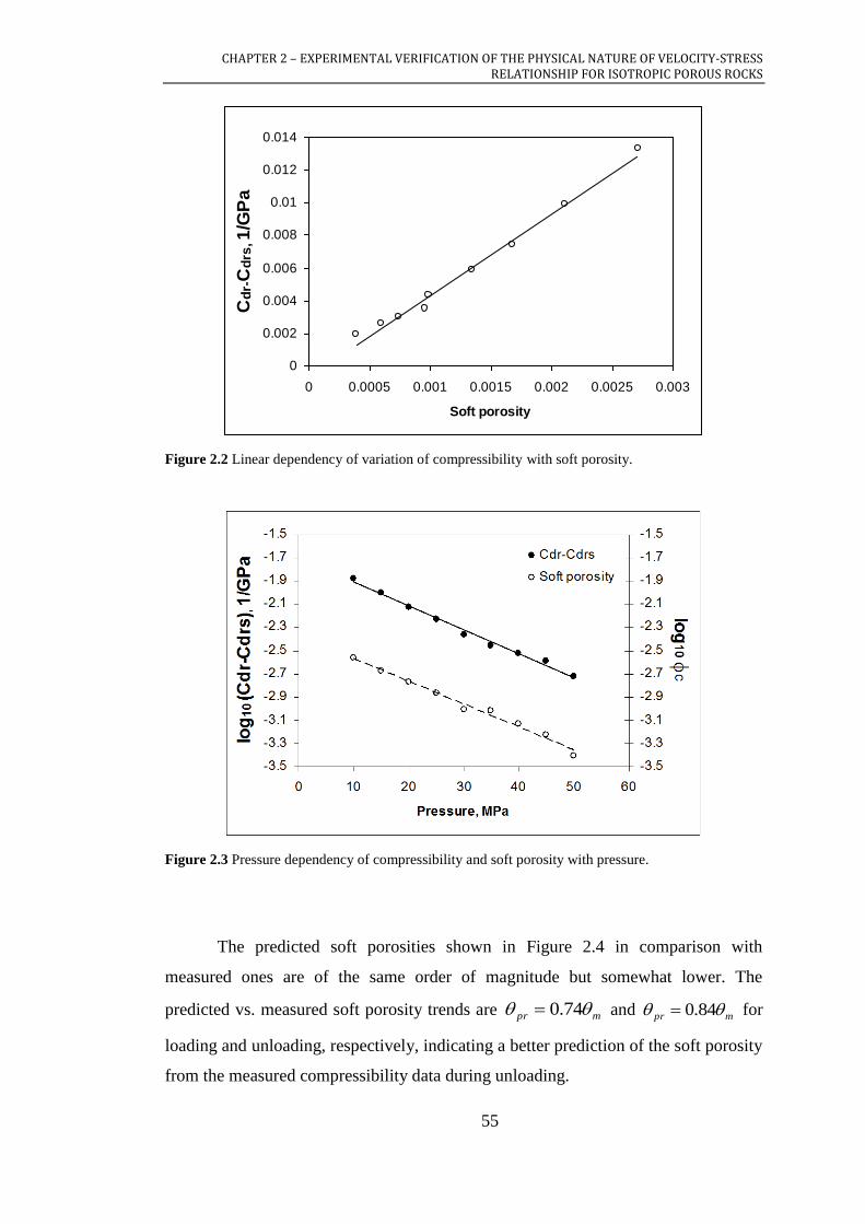
CHAPTER 2 – EXPERIMENTAL VERIFICATION OF THE PHYSICAL NATURE OF VELOCITY-STRESS RELATIONSHIP FOR ISOTROPIC POROUS ROCKS
55
Figure 2.2 Linear dependency of variation of compressibility with soft porosity.
Figure 2.3 Pressure dependency of compressibility and soft porosity with pressure.
The predicted soft porosities shown in Figure 2.4 in comparison with
measured ones are of the same order of magnitude but somewhat lower. The
predicted vs. measured soft porosity trends are mpr 74.0 and mpr 84.0 for
loading and unloading, respectively, indicating a better prediction of the soft porosity
from the measured compressibility data during unloading.
0
0.002
0.004
0.006
0.008
0.01
0.012
0.014
0 0.0005 0.001 0.0015 0.002 0.0025 0.003
Soft porosity
Cd
r-C
drs
, 1
/GP
a

CHAPTER 2 – EXPERIMENTAL VERIFICATION OF THE PHYSICAL NATURE OF VELOCITY-STRESS RELATIONSHIP FOR ISOTROPIC POROUS ROCKS
56
Figure 2.4 Correlation between predicted and measured soft porosities.
2.5 CHAPTER CONCLUSIONS
Theoretical interpretation of exponential stress dependency of elastic
properties of rocks based on a dual porosity concept has been tested using laboratory
measurements on dry sandstones. For those sandstone samples, the following
postulates of the theoretical model are shown to work well: (1) linear dependency of
elastic compressibility on soft porosity and (2) exponential decay of soft porosity and
elastic compressibility with effective stress up to 60 MPa. The magnitude of the
variation of stiff porosity with stress is shown to be comparable with compliant
porosity. However, this variation has a negligible effect on rock compressibility up to
60 MPa. Soft porosity estimated from the fitting coefficients of the elastic
compressibilities is on the same order of magnitude but slightly lower than obtained
from strain measurements. These results confirm the applicability of Shapiro’s
(2003) stress sensitivity model and hence provide justification for using this
approach to model the effect of stress on properties of both isotropic and anisotropic
rocks.

CHAPTER 3 – PARAMETERIZATION OF ELASTIC STRESS SENSITIVITY IN SHALES
57
CHAPTER 3 – PARAMETERIZATION OF ELASTIC STRESS SENSITIVITY IN SHALES
Stress dependency and anisotropy of dynamic elastic properties of shales is
important for a number of geophysical applications, including seismic interpretation,
fluid identification and 4D seismic monitoring. Using Sayers-Kachanov formalism,
we develop a new model for transversely isotropic (TI) media, which describes stress
sensitivity behaviour of all five elastic coefficients using four physically meaningful
parameters. The model is used to parameterize elastic properties of about 20 shales
obtained from laboratory measurements and from the literature. The four fitting
parameters, namely, specific tangential compliance of a single crack, ratio of normal
to tangential compliances, characteristic pressure and crack orientation anisotropy
parameter show moderate to good correlations with the depth from which the shale
was extracted. With increasing depth, the tangential compliance exponentially
decreases. The crack orientation anisotropy parameter broadly increases with depth
for most of the shales, indicating that cracks are getting more aligned in the bedding
plane. The ratio of normal to shear compliance and characteristic pressure decreases
with depth to 2500 m and then increases below this to 3600 m. The proposed model
allows evaluation of the stress dependency of all five elastic compliances of a TI
medium, even if only some of them are known. This may allow the reconstruction of
the stress dependency of all five elastic compliances of a shale from log data for
example.
This chapter is based on the published version of the following journal
publication with permission from co-authors and publishers (see Appendix B):
Pervukhina M., Gurevich B., Golodoniuc P., and Dewhurst D. N., 2011,
Parameterization of elastic stress sensitivity in shales: Geophysics, 76(3), p.
WA147–WA155, doi:10.1190/1.3554401.

CHAPTER 3 – PARAMETERIZATION OF ELASTIC STRESS SENSITIVITY IN SHALES
58
3.1 INTRODUCTION
Shales are the most common rock type encountered in sedimentary basins.
Due to their strongly anisotropic properties, the presence of shales in the subsurface
may cause significant errors in depth obtained from surface seismic data, in normal
moveout (NMO) correction, dip moveout correction (DMO), migration and
amplitude versus offset analysis (e.g., Castagna et al., 1993; Banik, 1984; Sayers,
1999; Tsvankin et al., 2009). Seismic anisotropy of shales is caused by a number of
factors, including intrinsic anisotropy of clay minerals that are abundant in shales,
preferred orientation of clay platelets, alignment of thin flat pores, and kerogen
inclusions (e.g., Hornby et al., 1994; Johnston and Christensen, 1995; Sayers, 1999).
Various studies have addressed the problem of prediction of shale anisotropy,
which requires values of the five elastic stiffness coefficients required to describe a
transversely isotropic (TI) medium and Thomsen’s anisotropy parameters (Thomsen,
1986). Johnston and Christensen (1995) reported a strong positive correlation
between seismic anisotropy and so-called orientation indices that reflected clay
mineral alignment. Johansen et al. (2004) studied the effect of alignment of grain
scale texture on seismic anisotropy and reflectivity of shales. Sayers (2005) related
the clay platelet orientation distribution to the behaviour of Thomsen’s parameter,
which is the only anisotropy parameter needed to interpret the small-offset amplitude
variation with offset (AVO) response. Using self-consistent approximation (SCA)
effective media theory, Hornby et al. (1994) reconstruct the TI elastic tensor of the
Greenhorn Shale on the basis of the knowledge of clay platelet orientation
distribution and silt inclusion fraction, assuming knowledge of clay elastic
properties. All these previous studies required knowledge of detailed microstructure
and assume that anisotropic the elastic moduli of individual clay minerals are known.
However, the clay platelet orientation characteristics, which require thorough
quantitative image analysis, can vary from sample to sample even for shale samples
acquired just a few meters apart. In addition, elastic properties of clay minerals
reported in the literature range in value by more than an order of magnitude (e.g.,
Aleksandrov and Ryzhova, 1961; Woeber et al., 1963; Han et al., 1986; Castagna et
al., 1993; Hornby et al., 1994; Katahara, 1996; Vanorio et al., 2003; Ortega et al.,
2007) and depend on a number of parameters such as clay mineralogy, water content
and sample preservation.

CHAPTER 3 – PARAMETERIZATION OF ELASTIC STRESS SENSITIVITY IN SHALES
59
Recently, Ulm and Abousleiman (2006) suggested a simple model that allows
prediction of anisotropic elastic moduli of shales. This model implies that shale
elastic properties are independent of clay mineralogy and allows prediction of elastic
moduli on the basis of only two parameters, namely, silt fraction and clay packing
density (CPD), a volumetric fraction of clay minerals in wet shale without silt
inclusions. Using this model in combination with the SCA approach, Ulm and
Abousleiman (2006) estimated elastic moduli of clay minerals from measurements of
elastic properties of a number of shales. Bayuk et al. (2007) used the general singular
approximation (GSA) effective media approach to estimate the elasticity tensor of
clay minerals from experimentally measured elastic properties of the Greenhorn
Shale used in Hornby’s study (Hornby et al., 1994). The approach of Ulm and
Abousleiman (2006) and Bayuk et al. (2007) was further refined by Pervukhina et al.
(2008a, 2008b) who suggested using a differential effective media (DEM) approach
as the most relevant for shale microstructure. The suggested method works quite well
for predicting anisotropic elastic moduli of shales based on CPD and silt fraction.
However, it fails to predict stress dependency of elastic properties of shales
(Pervukhina et al., 2008a, 2008b), which has been observed in many experiments
(e.g., Jakobsen and Johansen, 2000; Dewhurst and Siggins, 2006; Kuila et al., 2010;
Delle Piane et al., 2010).
The problem of stress dependency of shale properties is important for such
applications as pore pressure prediction, or time lapse seismic monitoring. Despite
this, there is no widely accepted theory for stress dependency of elastic properties of
shales. Sayers (1999) studied stress dependencies of air-dry and fluid-saturated
shales using the Sayers and Kachanov (1995) excess compliance approach and
obtained ratios of normal to tangential compliances of clay platelet contacts for the
both cases, assuming the contacts were well aligned. Prioul et al. (2004) and Prioul
and Lebrat (2004) described the stress dependency of shales using a model based on
non-linear elasticity with three stress-sensitive (nonlinear) parameters, although this
model is suitable only for a stress range where stiffnesses are quasi-linear with stress.
Shapiro and Kaselow (2005) suggested a stress dependency model for orthorhombic
media based on a dual porosity approach. Their model is based on the bimodal
distribution of pore compliances and superposition of deformation fields caused by
closure/shape change of these two groups of soft and stiff pores under applied stress.

CHAPTER 3 – PARAMETERIZATION OF ELASTIC STRESS SENSITIVITY IN SHALES
60
Ciz and Shapiro (2009) used this approach to build a model of experimental shale
measurements from the North Sea previously reported by Hornby (1998) and showed
a good model fit to the measurements. However in the isotropic limit, the model of
Ciz and Shapiro (2009) has been shown to be equivalent to the isotropic version of
the model of Sayers (1999) with exponential dependency of excess compliances on
pressure and with an additional assumption that normal and tangential compliances
of each grain contact are equal (Gurevich et al., 2009). This assumption may not be
physically adequate, especially for water-saturated rocks at ultrasonic frequencies,
since water in intergranular pores and microfractures should strongly reduce normal,
but not tangential, compliance.
Herein, a new model is proposed that allows description of stress dependency
of all five elastic coefficients of TI shales by treating both the orientation distribution
of clay platelets and the compliance ratio of platelet contacts as model parameters.
To this end, we combine the dual porosity approach of Shapiro and Kaselow (2005)
with the non-interactive approximation of Sayers and Kachanov (1995).
3.2 MODELLING OF THE EFFECT OF ISOTROPIC STRESS ON THE
ANISOTROPIC ORIENTATION OF DISCONTINUITIES
Following Shapiro (2003), Shapiro and Kaselow (2005) and Ciz and Shapiro
(2009), we assume that variation of elastic properties of a shale subjected to effective
confining pressures of up to 60 MPa can be explained by closure of soft (compliant)
porosity. Soft porosity comprises a small part of total porosity and consists of pores
with high compliances, such as fractures, cracks and grain or clay platelet contacts.
Figure 3.1 shows an SEM image, which illustrates existence of both stiff and
compliant pores in shales.
We model shale as an intrinsically transversely isotropic medium that is
permeated with discontinuities such as grain or platelet contacts, cracks or fractures,
which are distributed anisotropically. We assume that the probability density for a
particular orientation can be written as:
2 2
22
0 0
1 cos 1 cos,
4 1 31 cos sinW
d d
(3.1)

CHAPTER 3 – PARAMETERIZATION OF ELASTIC STRESS SENSITIVITY IN SHALES
61
where is an angle between the z-axis and the normal to the crack surface (range [0,
]), determines the rotation about the z-axis (range [0, 2]) and is the crack
orientation anisotropy parameter. Isotropic distribution of cracks corresponds to the
case when 0 and in the case when is large, there is a strong alignment of
cracks. One can check that the probability density defined by equation 3.1 satisfies
the normalization condition:
2
0 0, sin 1W d d
(3.2)
Figure 3.1 An Officer Basin shale showing particle alignment and the presence of microfractures
(white arrows). Modified from Kuila et al. (2010).

CHAPTER 3 – PARAMETERIZATION OF ELASTIC STRESS SENSITIVITY IN SHALES
62
The exact geometry of individual cracks is not specified. Instead, the
behaviour of cracks is defined by TB , the specific tangential compliance (tangential
compliance of a crack with a unit surface area) and a ratio /N TB B B where NB is
specific normal compliance. For parameterization purposes, only effective properties
are important, so the surface area A and the compliance ratio B are assumed to be the
same for all cracks. We assume that NB and
TB are independent of cracks
orientation and do not change with stress (for analysis of this assumption for
isotropic rocks, see Pervukhina et al., 2010). Following Schoenberg (2002), Shapiro
(2003) and Shapiro and Kaselow (2005), we further assume that the surface area of
individual cracks decreases with stress exponentially. Therefore, a specific surface
area per unit volume 0 0s N A also varies exponentially with stress, such that:
0
0 exp / cs P N A P P (3.3)
where N0 is the total number of cracks integrated over all angles, 0A is the specific
surface area of an individual crack at zero stress, P is effective stress and Pc is a
characteristic crack closing pressure.
When a rock with this distribution of discontinuities is subjected to a small
compressive isotropic stress, the density of cracks along a particular plane is assumed
to be reduced exponentially with the normal stress traction acting on that plane. The
area of the cracks in the case of their anisotropic distribution will reduce differently
in different directions. An effect of this anisotropic variation of the crack areas on
elastic properties can be modelled using the Sayers and Kachanov (1995) non-
interactive approximation:
0 1
4ijkl ijkl ijkl ik jl il jk jk il jl ik ijklS S S
(3.4)
( ) ( ) ( ) ( )1 r r r r
ij T i j
r
B n n AV
(3.5)
( ) ( ) ( ) ( ) ( ) ( ) ( )1 r r r r r r r
ijkl N T i j k l
r
B B n n n n AV
(3.6)

CHAPTER 3 – PARAMETERIZATION OF ELASTIC STRESS SENSITIVITY IN SHALES
63
Here, ijklS is the excess compliance caused by the presence of compliant
cracks, 0
ijklS are compliances at high stress with all soft cracks closed and ijklS are
the compliances at some intermediate stress; ij is the Kronecker delta; r is the
number of planar discontinuities with surface area ( )rA and ( )r
in and ( )r
jn are i-th and
j-th components of the unit vector that is normal to the surface of the rth grain
boundary in volume V; finally, NB and
TB are the normal and tangential
compliances of an individual crack.
Substituting equations 3.1 and 3.3 into equations 3.4-3.6, we obtain variation
in compliances due to the closure of discontinuities at different pressures as follows:
0
11 11 11
exp14 4 21 3
105
n T cs B P PS S S B B
(3.7)
0
33 33 33
exp14 6 21 15
105
n T cs B P PS S S B B
(3.8)
0
44 44 44
exp42 16 28 12
105
n T cs B P PS S S B B
(3.9)
0
66 66 66
exp42 10 28 4
105
n T cs B P PS S S B B
(3.10)
0
13 13 13
exp7 3 7 3
105
n T cs B P PS S S B B
. (3.11)
Here 4 1 3ns s and 0
0s N A is the specific surface area of cracks
per unit volume. The detailed derivation of equations 3.7-3.11 is given in Appendix
A. Note that shales exhibit TI anisotropy and five independent elastic compliances
S110, S33
0, S440, S66
0 and S130 are required even at high effect stresses when all
compliant cracks are supposed to be closed. Such intrinsic anisotropy is caused by
anisotropic individual clay mineral moduli and preferential orientation of domains of
aggregated clay minerals. If we assume N TB B , then equations 3.7-3.11 can be
simplified as follows:

CHAPTER 3 – PARAMETERIZATION OF ELASTIC STRESS SENSITIVITY IN SHALES
64
0
11 11 11
exp /5
15
n T cs B P PS S S
(3.12)
0
33 33 33
exp /5 3
15
n T cs B P PS S S
(3.13)
0
44 44 44
exp /10 4
15
n T cs B P PS S S
(3.14)
0
66 66 66
2 exp /5
15
n T cs B P PS S S
(3.15)
0
13 13 13 0S S S . (3.16)
Thus, to parameterize the stress dependency of shales for the general case,
when N TB B (i.e. equations 3.7-3.11 above), four parameters are necessary, namely
n Ts B , tangential compliance of an individual crack per unit area multiplied by the
normalized specific surface area of cracks per unit volume; B, the ratio of crack
normal to crack tangential compliance; η, the crack orientation anisotropy parameter
that characterizes angular crack distribution, and cP , the characteristic pressure at
which compliant pores close. For the case of so-called scalar crack approximation
when N TB B , three parameters n Ts B , η, cP are required. Note that the parameters
ns and TB are coupled and cannot be obtained independently. Hereafter, we refer to
n Ts B as TB bearing in mind that it is, in fact, multiplied by the normalized specific
surface area of cracks per unit volume. Below, we fit experimentally measured stress
dependencies of elastic properties of shales using both the general set of equations
3.7-3.11 and the scalar crack approximation (equations 3.12-3.16) and show the
uncertainties that are introduced in the latter case.
3.3 DATA
We applied our model to a number of shales from the Officer Basin, Bass
Basin, Carnarvon Basin (offshore Australia), Africa and the North Sea (Pervukhina
et al., 2008b). The details of the experimental procedure and sample preparation can
be found in Dewhurst and Siggins (2006) and Dewhurst et al. (2008a, 2008b). We

CHAPTER 3 – PARAMETERIZATION OF ELASTIC STRESS SENSITIVITY IN SHALES
65
also used stress dependencies measured by Wang (2002) on shale samples from
Africa, North Sea shales, Gulf Coast shale and hard shales. We used measurements
obtained for samples cut parallel and perpendicular to bedding, as application of an
isotropic stress would not change the TI symmetry of these samples. All the samples
were preserved (prevented from drying) before measurements. All the data were
obtained in the experiments with controlled pore pressure. The measurements for
shales from the Officer Basin, Bass Basin, Carnarvon Basin, Africa and the North
Sea were obtained under a pore pressure of 5 MPa. The pore pressures for other
shales are given in Wang (2002).
The shale samples were recovered from depths between 200 and 3604 m and
vary in their physical properties and in their mineralogy. Unfortunately, Wang (2002)
does not report information about overburden pressure, diagenesis, geological
history, clay content and mineralogy of the investigated shales. The depth of origin
of the shale samples is the only environmental parameter known for all the shales.
3.4 FITTING PROCEDURE AND TRENDS IN MICROCRACK PROPERTIES
The fitting procedure is schematically shown in Figure 3.2. Compliances
calculated from experimentally measured velocities at different isotropic effective
stresses are fitted using the sets of equations defined in 3.7-3.11 or 3.12-3.16. The
Levenberg-Marquardt method (Moré, 1977) is used for nonlinear fitting of
experimentally obtained stress dependencies of the elastic compliances of shales with
equations 3.7-3.11 or 3.12-3.16, considering BT, B, Pc and η as fitting parameters. We
first fit the data using the scalar crack approximation in equations 3.12-3.16 and then
use the resultant parameters BT, Pc and η and B = 1 as an initial estimate for the
general set of equations 3.7-3.11. For the second procedure, we use a condition B 2
as a constraint to fit the results.
A histogram of the compliance ratio, B, obtained using equations 3.7-3.11, is
shown in Figure 3.3. The values are distributed in three distinct groups, (i) small
values less than 0.2, (ii) normal values from 0.7-1.1 and (iii) large values of about 2.
Departure from unity is observed even in the group with the values from 0.7 to 1.1.
This suggests that the ratio B = 1 which corresponds to the model of Ciz and Shapiro
(2009) may not be adequate for shales.

CHAPTER 3 – PARAMETERIZATION OF ELASTIC STRESS SENSITIVITY IN SHALES
66
Figure 3.2 Schematic diagram of fitting procedure. Compliances calculated from experimentally
measured velocities at different isotropic effective stresses are fitted using a set of equations 3.7-3.11.
As a result of the fitting, four fitting parameters are obtained.
Figure 3.3 Histogram of the ratio of normal to tangential compliance for all the shale samples. Most
of the values are far from unity.

CHAPTER 3 – PARAMETERIZATION OF ELASTIC STRESS SENSITIVITY IN SHALES
67
To understand the excess in misfit of the experimental stress dependencies
caused by the assumption that B = 1, we compare the results of the experimental data
fitting using equations 3.7-3.11 and 3.12-3.16. The misfits are shown in Figure 3.4a
by solid dots (equations 3.7-3.11) and open circles (equations 3.12-3.16). Figure 3.4b
shows the relative excess of misfit caused by the assumption that N TB B . The
relative misfits are close to zero and consequently the misfits are almost the same
when B is close to unity. However in other cases, the misfit by equation set 3.12-3.16
noticeably exceeds the one obtained by use of equations 3.7-3.11 (note that the plot
in Figure 3.4a is in logarithmic scale). The error caused by use of a scalar crack
approximation (equations 3.12-3.16) exceeds the error resulted from fitting with the
full set of equations 3.7-3.11 by up to 70%. Similar results were obtained by Angus
et al. (2009) who used a synthetic data set to estimate an error caused by usage of a
scalar crack approximation instead of the full set of equations. From here onwards,
we use only equation set 3.7-3.11 to fit the experimental stress dependencies of
elastic properties of shales to avoid additional errors caused by the assumption that
N TB B .
All four fitting parameters are plotted versus depth of shale extraction in
Figure 3.5. Crack orientation anisotropy parameter, η, shows a general linear growth
with depth of origin (Figure 3.5a) although there is significant scatter of the fitting
values. Higher values of η mean better alignment of the cracks in the bedding plane;
consequently, an increase of η with the depth indicates increased alignment of
discontinuities with increasing overburden pressure.
Tangential compliance of a single crack normalized to the area of the crack
exponentially decreases with depth (Figure 3.5b). This implies that cracks are stiffer
in shales that are recovered from greater depths than in the shales extracted from
shallower depths.
The ratio of normal to tangential compliance initially decreases from 1 to 0.1
with the increase of depth from 1000 to 2500 m (Figure 3.5c), implying that normal
stiffness of shales grows faster with the overburden pressure than the tangential one.
Then B increases again reaching 2 at the depth of 3500 m. In other words, in the
depth range of 1000-2500 m, cracks become relatively stiffer in the plane of the
crack than in the normal direction with increasing depth. However, below 2500 m,
the reverse seems to occur. While it is commonly accepted that individual shales can
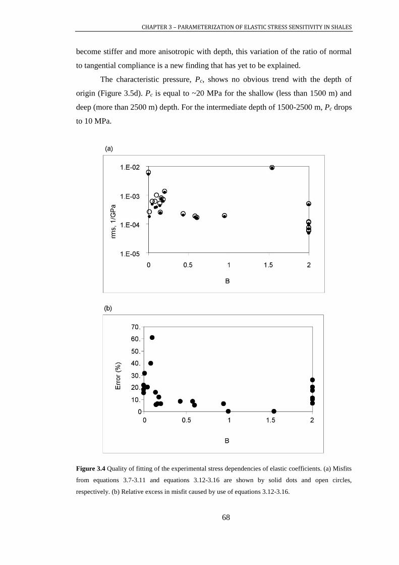
CHAPTER 3 – PARAMETERIZATION OF ELASTIC STRESS SENSITIVITY IN SHALES
68
become stiffer and more anisotropic with depth, this variation of the ratio of normal
to tangential compliance is a new finding that has yet to be explained.
The characteristic pressure, Pc, shows no obvious trend with the depth of
origin (Figure 3.5d). Pc is equal to ~20 MPa for the shallow (less than 1500 m) and
deep (more than 2500 m) depth. For the intermediate depth of 1500-2500 m, Pc drops
to 10 MPa.
Figure 3.4 Quality of fitting of the experimental stress dependencies of elastic coefficients. (a) Misfits
from equations 3.7-3.11 and equations 3.12-3.16 are shown by solid dots and open circles,
respectively. (b) Relative excess in misfit caused by use of equations 3.12-3.16.
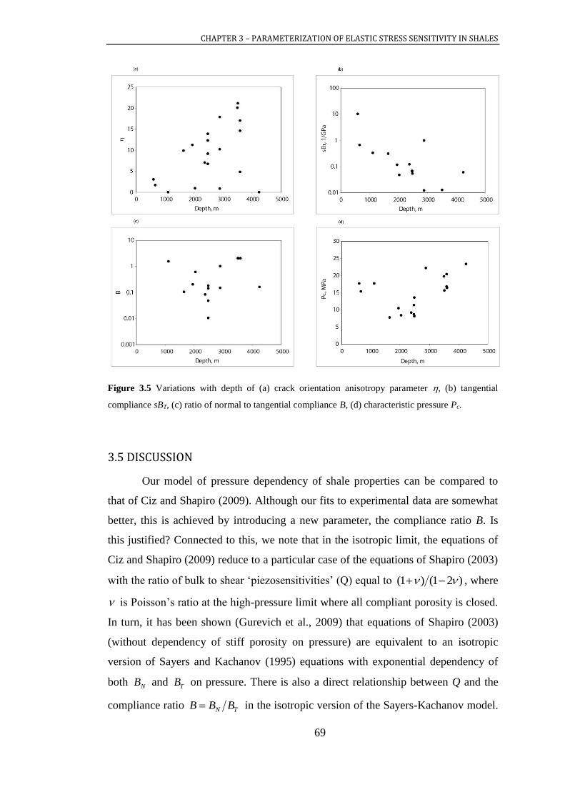
CHAPTER 3 – PARAMETERIZATION OF ELASTIC STRESS SENSITIVITY IN SHALES
69
Figure 3.5 Variations with depth of (a) crack orientation anisotropy parameter , (b) tangential
compliance sBT, (c) ratio of normal to tangential compliance B, (d) characteristic pressure Pc.
3.5 DISCUSSION
Our model of pressure dependency of shale properties can be compared to
that of Ciz and Shapiro (2009). Although our fits to experimental data are somewhat
better, this is achieved by introducing a new parameter, the compliance ratio B. Is
this justified? Connected to this, we note that in the isotropic limit, the equations of
Ciz and Shapiro (2009) reduce to a particular case of the equations of Shapiro (2003)
with the ratio of bulk to shear ‘piezosensitivities’ (Q) equal to (1 ) (1 2 ) , where
is Poisson’s ratio at the high-pressure limit where all compliant porosity is closed.
In turn, it has been shown (Gurevich et al., 2009) that equations of Shapiro (2003)
(without dependency of stiff porosity on pressure) are equivalent to an isotropic
version of Sayers and Kachanov (1995) equations with exponential dependency of
both NB and TB on pressure. There is also a direct relationship between Q and the
compliance ratio N TB B B in the isotropic version of the Sayers-Kachanov model.

CHAPTER 3 – PARAMETERIZATION OF ELASTIC STRESS SENSITIVITY IN SHALES
70
In particular, (1 ) (1 2 )Q corresponds to 1B (Gurevich et al. 2009,
equation 10). While improvement of the fit by allowing B to be a free parameter may
not be huge, we think that assumption 1B may not be physically adequate,
especially for water-saturated rocks at ultrasonic frequencies, since water in
intergranular microcracks should strongly reduce NB but not
TB . For isotropic rocks,
this has been confirmed by analysis of laboratory measurements (see Sayers and
Han, 2002, and Angus et al., 2009). We believe this is also logical for anisotropic
rocks, including shales, even if quality of shale data may not be sufficient at present
to show this conclusively. We also note that even with a new parameter B, our model
still has fewer parameters than the model of Ciz and Shapiro (2009).
The developed model allows one to obtain statistically qualitative properties
of microcracks in shales. For the analysed dataset, these properties show moderate to
good correlations with the depth of extraction. Even though some of the parameters
exhibit only a broad correlation with the depth of origin, such general correlations for
shales may be helpful for initial characterisation of stress dependencies of elastic
properties of shales in new basins. Thus, we believe that more extensive and
statistically representative studies are required to confirm, improve (if possible) and
understand the physical meaning of the obtained broad correlations. For example, it
is well known that stress history and temperature also control mechanical and elastic
properties of shales (e.g., Nygard et al., 2004; Peltonen et al., 2009) through
poroelastic effects and diagenetic mineral reactions respectively. Unfortunately, such
data were not available for most of the shales evaluated, so we were unable to
characterize the shales more specifically in these terms at this stage. However, even
with this restriction, the model gives some results that seem geologically intuitive,
suggesting a physically sound basis for further development.
From analysing this limited dataset, one can conclude that the crack
orientation anisotropy parameter shows only a broad correlation with the depth.
While clay particle orientation and associated microfractures are often seen as
dependent on overburden stress, this can also occur through other less well defined
processes that are not governed by depth alone. In addition, clay alignment also can
depend on the volume of the silt fraction and the shape of silty grains, which may
result in differential compaction of clays and wrapping around more rigid particles.

CHAPTER 3 – PARAMETERIZATION OF ELASTIC STRESS SENSITIVITY IN SHALES
71
Hence, larger datasets may not drastically improve the correlation between and
depth of extraction or overburden pressure.
Shear compliance (BT) shows a good correlation with depth of extraction
(Figure 3.5b). More complex behaviour is observed for the ratio of normal to
tangential compliance B (Figure 3.5c) in that it decreases from 1 to 0.1 between 1000
and 2500 m and then increases above unity to 3600 m. This may reflect the effects of
diagenesis that generally starts at the depth of about 2000-3000 meters, driven by
temperatures above 65˚C (Ruud et al., 2003; Avseth et al., 2008; Storvoll and Brevik,
2008). It should be noted that the ratio of normal to tangential compliance in a given
rock will reflect the roughness of the crack surfaces and this might be affected by
mineralization. The values of B estimated for real rocks often exceed theoretical
predictions for traction-free cracks (which always yields B < 1). In particular, Angus
et al. (2009) observed values of N TB B up to 1.75 for dry shales. MacBeth and
Schuett (2007) found that the ratio B may increase to the values above unity for
thermally damaged samples. Possible contact mechanisms and the effect of
mineralization on the values of B are discussed in detail in Sayers et al. (2009) and
Kachanov et al. (2010). The characteristic stress, Pc, also shows a minimum in
absolute values at depths of ~2500 m, similar to that observed for B; this may
support our speculative suggestion that the microcrack parameters reflect the effects
of mechanical compaction and diagenesis undergone by a particular shale sample.
More data and detailed information on shale mineralogy and microstructure are
required to test these observations.
The model we have developed can also be used for predicting the stress
dependency of unknown elastic parameters from the known ones. This problem is
practically important either for laboratory measurements in shales, where the C13
coefficient is often unreliable and, for the field data analysis, where log data only
allow determination of up to four out of five elastic coefficients of TI media (Sinha et
al., 2006). Note that the fitting problem described by equations 3.7-3.11 is
overdetermined (see Figure 3.2). Elastic compliances used for the fitting are
calculated for each effective stress at which ultrasonic velocities were measured. For
instance if ultrasonic velocities were measured at np effective stresses, we have 5np
equations in total. Thus, the four fitting parameters might be determined from
experimental stress dependencies of an incomplete set of elastic coefficients. If, for
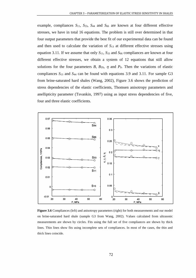
CHAPTER 3 – PARAMETERIZATION OF ELASTIC STRESS SENSITIVITY IN SHALES
72
example, compliances S11, S33, S44 and S66 are known at four different effective
stresses, we have in total 16 equations. The problem is still over determined in that
four output parameters that provide the best fit of our experimental data can be found
and then used to calculate the variation of S13 at different effective stresses using
equation 3.11. If we assume that only S11, S33 and S66 compliances are known at four
different effective stresses, we obtain a system of 12 equations that still allow
solutions for the four parameters B, BT0, and P0. Then the variations of elastic
compliances S13 and S44 can be found with equations 3.9 and 3.11. For sample G3
from brine-saturated hard shales (Wang, 2002), Figure 3.6 shows the prediction of
stress dependencies of the elastic coefficients, Thomsen anisotropy parameters and
anellipticity parameter (Tsvankin, 1997) using as input stress dependencies of five,
four and three elastic coefficients.
Figure 3.6 Compliances (left) and anisotropy parameters (right) for both measurements and our model
on brine-saturated hard shale (sample G3 from Wang, 2002). Values calculated from ultrasonic
measurements are shown by circles. Fits using the full set of five compliances are shown by thick
lines. Thin lines show fits using incomplete sets of compliances. In most of the cases, the thin and
thick lines coincide.

CHAPTER 3 – PARAMETERIZATION OF ELASTIC STRESS SENSITIVITY IN SHALES
73
The fitting parameters , B, sBT, P0 are 20, 2, 0.007 GPa-1 and 20 MPa. The
predictions obtained from input of four elastic coefficients (S11, S33, S44, S66) are
almost indistinguishable from those obtained for the input of five; the differences for
the case of input of three elastic coefficients (S11, S33, S66) are also small. However, it
is important to note explicitly that this prediction does not include prediction of the
intrinsic compliances 0
ijS , nor of the stress dependence due to the hard compliance at
large effective stress.
3.6 CHAPTER CONCLUSIONS
A new stress dependency model for TI media was developed and used to
parameterize stress dependencies of the elastic properties of about 20 shales. The
four fitting parameters (namely, specific tangential compliance of a single
discontinuity, ratio of normal to tangential compliances, characteristic pressure and
crack orientation anisotropy parameter) show moderate correlations with the depth
from which the shale was extracted. With increasing depth, the tangential compliance
exponentially decreases. The crack orientation anisotropy parameter broadly
increases with the depth for most of the shales, indicating that cracks are becoming
more aligned. The ratio of normal to shear compliance as well as characteristic
pressure decrease to depths of 2500 m and then increase below this to 3600 m. The
suggested model also allows the prediction of stress dependency of all five elastic
compliances if only three or four compliances are known. This could be useful for
the reconstruction of stress dependencies of all five elastic compliances of shale from
log data, for example.

CHAPTER 4 – STRESS DEPENDENCY OF ELASTIC PROPERTIES OF SHALES: THE EFFECT OF UNIAXIAL STRESS
74
CHAPTER 4 – STRESS DEPENDENCY OF ELASTIC PROPERTIES OF SHALES: THE EFFECT OF UNIAXIAL STRESS
Along with intrinsic anisotropy caused by preferred mineral orientation that is
common in shales, anisotropic stress is an important factor that affects shale elastic
response. While variations of elastic coefficients with anisotropic stress have been
the subject of experimental studies, theoretical insight is still largely lacking. Here,
we further extend the model proposed in Chapter 3 to the case where shales are
subjected to uniaxial stress, which allows parameterization of the stress dependency
of elastic coefficients of shales under anisotropic stress conditions. We show that
parameterization requires four parameters, namely, specific tangential compliance of
a single crack, the ratio of normal to tangential compliances, characteristic pressure,
and a crack orientation anisotropy parameter. These parameters can be estimated
from experimentally measured stress sensitivity of elastic coefficients in shales to
isotropic stress.
In this chapter, I used the material published in the following SEG extended
abstract with permission from co-authors and publishers (see Appendix B):
Pervukhina M., Gurevich B., Golodoniuc P., and Dewhurst D. N., 2011,
Stress dependency of elastic properties of shales: the effect of uniaxial stress:
SEG Extended abstract at the SEG 2011 Conference, San Antonio, USA,
doi:10.1190/1.3627669.
4.1 INTRODUCTION
The effect of stress on elastic properties of shales is also important for
understanding of depositional trends especially at the upper 2000-3000 meters where
the compaction is mostly mechanical. Despite the importance of the effects of
isotropic and especially anisotropic stress on elastic properties of shales, little work
has been done on theoretical understanding and predicting such properties and
generally for the case of isotropic stress. All the existing theoretical approaches to
the problem of elastic stress sensitivity are based on the analysis of orientation
distribution of discontinuities and their normal, BN, and shear, BT, compliances.
Sayers (1999) studied stress-dependent seismic anisotropy of shales using ultrasonic
CHAPTER 4 – STRESS DEPENDENCY OF ELASTIC PROPERTIES OF SHALES: THE EFFECT OF UNIAXIAL STRESS
75
measurements on two fully saturated shales of Jurassic age reported by Hornby et al.
(1994), two air-dry shales from the Millboro and Braillier members of the Devonian-
Mississipian Chattanooga Formation (Johnston and Christensen, 1993) and air-dry
mature, kerogen-rich shale (Vernik, 1993). Sayers used the formalism presented in
Sayers and Kachanov (1995) that takes into account extra compliance induced by
fractures and cracks. Sayers (1999) calculated BN / BT ratios for each point of
confining stress assuming that the discontinuities are perfectly aligned. Analysing the
experimentally obtained stress dependencies of the five elastic coefficients, Sayers
(1999) concluded that the contacts between clay particles are more compliant in
shear than in compression and the ratios of normal to tangential compliances of
individual cracks are higher for the air-dry shales compared to those in saturated
shales.
Ciz and Shapiro (2009) studied the variations of elastic compliances and
anisotropic parameters of Jurassic North Sea shale with isotropic stress reported in
Prioul et al. (2004). They applied the so-called porosity deformation model (also
known as dual porosity model, stress-sensitivity or piezo-sensitivity) initially
developed by Shapiro (2003) for dry isotropic rock and later extended by Shapiro
and Kaselow (2005) to the case of orthorhombic symmetry. Ciz and Shapiro (2009)
described stress dependency of all elastic coefficients apart from S13, which is
independent of stress in the porosity deformation model. As laboratory
measurements commonly show noticeable variations in S13 with pressure, this is a
limitation of the porosity deformation model. The Sayers-Kachanov model seems to
be more universal.
Using the Sayers-Kachanov model, Gurevich et al. (2011) suggested a new
analytical model of stress induced anisotropy caused by application of uniaxial stress
to an isotropic cracked medium. Using a similar approach, we developed a new
model for stress dependency of transversely isotropic (TI) media in Chapter 3, which
predicts stress sensitivity behaviour of all five elastic coefficients using four
physically plausible parameters. These are the specific tangential compliance of a
single crack, the ratio of normal to tangential compliances, the characteristic pressure
and a crack orientation anisotropy parameter. The model has been used to
parameterize elastic properties of about 20 shales. The four fitting parameters
showed moderate to good correlations with the depth from which the shale was

CHAPTER 4 – STRESS DEPENDENCY OF ELASTIC PROPERTIES OF SHALES: THE EFFECT OF UNIAXIAL STRESS
76
extracted. With increasing depth, the tangential compliance exponentially decreases.
The crack orientation anisotropy parameter broadly increases with the depth for most
of the shales, indicating that cracks are getting more aligned in the bedding plane.
The ratio of normal to shear compliance and characteristic pressure decrease with the
depth to 2500 m, and then increase in the depth range of 2500-3600 m. The
suggested model also allows prediction of the stress dependency of all five elastic
compliances of a TI medium, even if only some of them are known.
This study extends the model developed earlier in Chapter 2 and Chapter 3 to
anisotropic (uniaxial) stresses. We show that at small uniaxial stresses, these effects
can be described using the same four parameters. Moreover, the values of these
parameters can be extracted from the experimental measurements obtained at
isotropic stress. Predictions of the model are compared with experimental
measurements.
4.2 MODELLING THE EFFECT OF ANISOTROPIC STRESS ON ELASTIC
COEFFICIENTS OF SHALES
Continuing the study we have conducted earlier in Chapter 3, we model the
shale as an intrinsically transversely isotropic medium that is permeated with
discontinuities (cracks or fractures). We assume an anisotropic orientation
distribution of discontinuities for which the probability density for a particular
orientation can be written as:
2 2
22
0 0
1 cos 1 cos,
4 1 31 cos sinW
d d
(4.1)
where is an angle between the z-axis and the normal to the crack surface (range [0,
]), determines the rotation about the z-axis (range [0, 2]) and is the crack
orientation anisotropy parameter. An isotropic distribution of cracks corresponds to
the case where 0 and in the case when is large, there is a strong alignment of
cracks. One can check that the probability density defined by equation 4.1 satisfies
the normalization condition:
2
0 0, sin 1W d d
(4.2)
CHAPTER 4 – STRESS DEPENDENCY OF ELASTIC PROPERTIES OF SHALES: THE EFFECT OF UNIAXIAL STRESS
77
Both here and below, the z-axis is chosen as a symmetry axis of the TI
medium. The exact geometry of individual cracks is not specified. Instead, the
behaviour of cracks is defined by a ratio B of the normal BN to tangential BT excess
crack compliances. All cracks are assumed identical; thus, B is the same for all
cracks.
The medium can undergo a zero or nonzero isotropic stress. The effect of the
nonzero isotropic stress on shale can be taken into account by assuming an
exponential reduction of crack area A(r) (and specific area of cracks s =A(r)/V) with
effective pressure P (confining pressure minus pore pressure) as follows:
0 exp / cs s P P
(4.3)
where s0 is specific area of all the cracks at zero pressure and Pc is a characteristic
crack closing pressure (Schoenberg, 2002; Shapiro, 2003; Shapiro and Kaselow,
2005; Vlastos et al., 2006).
When the rock is subjected to a small uniaxial compressive stress (σ) in
addition to an isotropic stress, the density of cracks along a particular plane is
reduced in proportion to the normal stress traction acting on that plane. To model
closure of cracks due to application of anisotropic stress, we can assume that r
NB
and r
TB are the same for all orientations of cracks, while A(r) (and specific area of
cracks s =A(r)/V) varies with direction of the crack normal, depending on the normal
stress acting in that direction:
0 exp / cs s P (4.4)
When uniaxial stresses are small compared to Pc, the exponential expression
in equation 4.4 can be approximated by a linear expression:
0 1 / cs s P (4.5)
The uniaxial stress does not change the TI symmetry of the shale if it is
applied along its symmetry axis (z-axis in our case). The variation of elastic
compliances with the applied isotropic and uniaxial stresses can be calculated using
Sayers-Kachanov model as follows:

CHAPTER 4 – STRESS DEPENDENCY OF ELASTIC PROPERTIES OF SHALES: THE EFFECT OF UNIAXIAL STRESS
78
0 1
4ijkl ijkl ijkl ik jl il jk jk il jl ik ijklS S S (4.6)
( ) ( ) ( ) ( )1 r r r r
ij T i j
r
B n n AV
(4.7)
( ) ( ) ( ) ( ) ( ) ( ) ( )1 r r r r r r r
ijkl N T i j k l
r
B B n n n n AV
(4.8)
Here, ijklS is the excess compliance caused by the presence of compliant
cracks, 0
ijklS are compliances at high stress with all soft cracks closed and ijklS are the
compliances at some intermediate stress; ij is the Kronecker delta; r is the number
of planar discontinuities with surface area ( )rA and
( )r
in and ( )r
jn are i-th and j-th
components of the unit vector that is normal to the surface of the r-th grain boundary
in volume V; finally, NB and TB are the normal and tangential compliances of an
individual crack.
Substituting equations 4.1, 4.3 and 4.5 together into equations (4.6-4.8), we
can obtain variations of five elastic compliances for a TI fractured medium that is
subject to both pressure (P) and uniaxial stress () parallel to the symmetry axis of
the TI medium. The derivation of the equations can be done following the procedure
that is described in detail in Chapter 3.
Here we restrict our study to the case of constant effective pressure P and
calculate variations of elastic compliances with variation of only anisotropic stress σ.
The formulae below express the variations in terms of the four parameters as follows:
11 0 4 2 3105
c
P
Pan
T
c
S B e B BP
(4.9)
33 0 18 10 45 35315
c
P
Pan
T
c
S B e B BP
(4.10)
13 0 9 5 9 5315
c
P
Pan
T
c
S B e B BP
(4.11)
44 0
224 17 18 10
315c
P
Pan
T
c
S B e B BP
(4.12)
66 0
215 7 6 2
315c
P
Pan
T
c
S B e B BP
. (4.13)

CHAPTER 4 – STRESS DEPENDENCY OF ELASTIC PROPERTIES OF SHALES: THE EFFECT OF UNIAXIAL STRESS
79
Here we employ the conventional matrix notation (e.g., Nye, 1985), which assumes
that:
mn ijklS S , when m and n are 1, 2, or 3;
2mn ijklS S , when m or n is 4, 5, or 6;
4mn ijklS S , when both m and n are 4, 5, or 6.
Note that the four parameters in equations 4.9-4.13 are the same as in the case
of isotropic stress and hence can be determined from the isotropic experiments. Thus,
the variations of elastic properties of shales if an anisotropic stress is applied can be
predicted from the variations that occur when the shale is subjected to an isotropic
stress. Here we show the applicability of this approach using experimental
measurements made on a shale from the onshore Officer Basin in Western Australia
(Kuila et al., 2010).
4.3 VALIDATION ON EXPERIMENTAL DATA
We compare ultrasonic velocities that were measured in a multistage triaxial
test on a shale sample from the Officer Basin with predictions from the theoretical
model. The Officer Basin shales are red shales of low porosity, comprising mainly
illite, orthoclase and quartz. These shales are laminated and in parts are rigid grain
supported. The sample of interest is extracted from the depth of 603 m and has a
porosity of 6%, clay fraction of 17% and clay content of 41%. It consists of quartz
(25%), orthoclase (29%), illite (35%), albite (4%), chlorite (4%), kaolinite (2%) and
haematite (2%). The sample is cut perpendicular to the bedding and thus, the
application of a uniaxial stress normal to the bedding does not change the TI
symmetry of the sample.
The ultrasonic experiments were done on a preserved, saturated shale sample
with controlled pore pressure. Firstly, a confining pressure is increased to some level,
for instance 20 MPa, and pore pressure is equilibrated at, for instance, 5 MPa, then
the axial stress is increased by increments, for instance, to 1, 2, 5, 8 and 15 MPa. The
details of the experimental procedure and sample preparation can be found in Kuila
et al. (2010).

CHAPTER 4 – STRESS DEPENDENCY OF ELASTIC PROPERTIES OF SHALES: THE EFFECT OF UNIAXIAL STRESS
80
The theoretical predictions made using formulas 4.9-4.13 and model
parameters B = 0.2, BT = 7 MPa-1 = 4 and Pc = 57 MPa were obtained from
isotropic measurements (refer to Chapter 3 for further details). In Figure 4.1, the
measured and predicted variations in P- and S-wave velocity due to variations of
axial stress are shown for effective pressures of ~10 MPa. In Figure 4.2 (a, b), P- and
S-wave velocities are shown as a function of angle of incidence for the same
effective stress and axial stresses of 1, 8 and 15 MPa.
Figure 4.1 Vph (circles), Vsh (diamonds), Vpv (squares) and Vs1 (triangles) velocities measured at 10
MPa of effective pressure in Officer Basin shale compared with model predictions (solid lines).
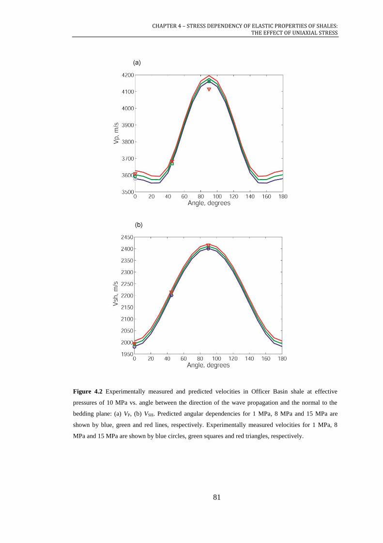
CHAPTER 4 – STRESS DEPENDENCY OF ELASTIC PROPERTIES OF SHALES: THE EFFECT OF UNIAXIAL STRESS
81
Figure 4.2 Experimentally measured and predicted velocities in Officer Basin shale at effective
pressures of 10 MPa vs. angle between the direction of the wave propagation and the normal to the
bedding plane: (a) VP, (b) VSH. Predicted angular dependencies for 1 MPa, 8 MPa and 15 MPa are
shown by blue, green and red lines, respectively. Experimentally measured velocities for 1 MPa, 8
MPa and 15 MPa are shown by blue circles, green squares and red triangles, respectively.
CHAPTER 4 – STRESS DEPENDENCY OF ELASTIC PROPERTIES OF SHALES: THE EFFECT OF UNIAXIAL STRESS
82
4.4 DISCUSSION
Both theoretical predictions and measurements show moderate dependency of
velocities with the uniaxial stress: this dependency gets weaker with an increase of
effective stress. While uniaxial stress increases from 0 to 8 MPa, VP and VS increase
by ~20 m/s at effective stresses of 10-20 MPa and even by a smaller amount at
higher stresses. The model predicts maximal variations in VP when the wave
propagates perpendicular to the bedding plane, while VS increases in both directions
(parallel and perpendicular to the bedding plane). Variations in the uniaxial stress
have the smallest effect on acoustic wave propagation in oblique directions.
However, these conclusions are valid for this particular shale and need to be verified
on other shales before application.
The developed model predicts well the variations in velocities due to the
application of uniaxial stress at small values (< 10 MPa) of the uniaxial stress. At
higher values of uniaxial stress, the model overestimates experimentally measured
velocities, which show no further increase and can even decrease with increasing
uniaxial stress. This is probably caused by opening of cracks parallel to the applied
direction of the uniaxial stress which is known to reduce velocities in shale samples
(Sayers, 1988; Dewhurst and Siggins, 2006; Kuila et al., 2010). The model presented
here is not designed for prediction of such effects and is thus applicable to small
axial stress variations ( cP ) only, due to the assumed linear closure of
discontinuity areas with stress (equation 4.5).
It is worth emphasizing again that the four parameters used in the model are
derived from the dependency of the elastic properties of the shale on isotropic stress
and are nevertheless shown to the given an adequate prediction of variation in elastic
properties under uniaxial stress. This fact implies that the model captures the essence
of the stress dependency mechanism and the proposed four parameters can be used to
parameterize stress sensitivity of different rock types.
The model can be used to analyse stress-related anisotropy in shales in situ
where stress perturbations are small and the corresponding variation in elastic moduli
can be assumed linear. For the general case of large stresses, when density of the
cracks cannot be considered reducing linearly, an analytical solution is not feasible
and numerical solution is required. However, experimental measurements in shales
show that for many samples, linear variation of compliances with stress is a

CHAPTER 4 – STRESS DEPENDENCY OF ELASTIC PROPERTIES OF SHALES: THE EFFECT OF UNIAXIAL STRESS
83
reasonable approximation and our model can be used to analyse the experimental
data for a moderate range of applied uniaxial stresses. The stress range that can be
investigated increases with shale strength.
4.5 CHAPTER CONCLUSIONS
A new model for prediction of elastic properties variation due to application
of uniaxial stress for TI media with discontinuities has been developed. The model
has been tested on experimental data obtained for a shale sample from the Officer
Basin in Western Australia. The predicted variations in elastic velocities are in a
good agreement with experimentally measured data. The developed model can be
used for prediction of elastic properties response to application of a small uniaxial
stress normal to the bedding plane when only variation of elastic properties with
isotropic stress is known.
CHAPTER 5 – PREDICTION OF SONIC VELOCITIES IN SHALE FROM POROSITY AND CLAY FRACTION OBTAINED FROM LOGS
84
CHAPTER 5 – PREDICTION OF SONIC VELOCITIES IN SHALE FROM POROSITY AND CLAY FRACTION OBTAINED FROM LOGS
Prediction of sonic velocities in shales from well logs is important for seismic
to log ties, when sonic log is absent for a shaly section, for pore pressure anomaly
detection, and for data quality control. Anisotropic elastic coefficients of the wet
clay, a hypothetic composite material that includes all clay and water of the shale but
exclude silt inclusions, are assumed as a first order approximation to be linearly
dependent on wet clay porosity. Here by the wet clay porosity, we mean a ratio of a
pore volume occupied by water to a total volume of the wet clay, where the former is
calculated from bulk and grain densities. Effects of silt inclusions on elastic
coefficients of shales are taken into account by using the anisotropic differential
effective medium (DEM) model. Silt inclusions are modelled as spherical quartz
particles. Simulated elastic coefficients of shales are used to calculate compressional
and shear velocities and compared with the sonic velocities observed on a test dataset
from a well penetrating a 500 m vertical section of shale.
To further study elastic properties of clays, elastic coefficients of shales are
inverted for vertical profiles of clay elastic coefficients. The analysis of these
coefficients shows that in the considered well, the increase in elastic coefficients of
shales is controlled by the increase of silt fraction with depth. Elastic coefficients of
clay show no increase with depth. Compared to the elastic moduli of shale, the
inverted elastic moduli of wet clay show much stronger correlation with clay
porosity, which confirms the hypothesis that silt fraction is one of the key parameters
for modelling of elastic properties of shale.
In this chapter, I used the material previously published in the following
EAGE and SEGJ extended abstracts, and that was later published in the Geophysics
in 2015. All published materials were used with permission from leading co-authors
and respective publishers (see Appendix B):
Pervukhina M., Golodoniuc P., Gurevich B., Clennell M. B., Nadri D.,
Dewhurst D. N., and Nordgård Bolås H. M., 2012, An estimation of sonic
velocities in shale from clay and silt fractions from the Elemental Capture
Spectroscopy log: Extended abstract, 74th EAGE Conference, Copenhagen,
Denmark.

CHAPTER 5 – PREDICTION OF SONIC VELOCITIES IN SHALE FROM POROSITY AND CLAY FRACTION OBTAINED FROM LOGS
85
Pervukhina M., Golodoniuc P., and Dewhurst D. N., 2013, Rock physics
modeling of sonic velocities in shales: Proceedings of the 11th SEGJ
International Symposium, Yokohama, Japan, 398-401.
Pervukhina M., Golodoniuc P., Gurevich B., Clennell M. B., Dewhurst D. N.,
and Nordgård Bolås H. M., 2015, Prediction of sonic velocities in shale from
porosity and clay fraction obtained from logs – a North Sea well case study:
Geophysics, 80(1), p. D1-D10, doi:10.1190/GEO2014-0044.1.
5.1 INTRODUCTION
Shales have been largely neglected in the past as barren overburden but have
attracted considerable interest in recent years as reservoirs, source rocks and seals. In
particular, knowledge of the factors that control elastic properties of shales is
important for their characterisation from surface and borehole seismic data.
Knowledge of elastic properties of shales and the parameters controlling those
properties is important for the quantitative seismic data interpretation, pore pressure
prediction and seismic anisotropy estimation. Most studies of shale properties are
based on very laborious and time-consuming ultrasonic measurements on preserved
shale samples. These samples give a very sparse representation of ubiquitous shaly
sediments in the subsurface. Thus it would be useful to predict elastic properties of
shales from their characteristics derived from well log data. The main objective of
this chapter is to develop a methodology for predicting elastic properties of shales
from their porosity and composition derived from logs, and to test and calibrate this
approach against sonic log data.
Shales are highly heterogeneous multi-scale rocks with micro-scale silt
inclusions, nano-scale porosity and various clay minerals as a host matrix. Despite
the fact that elastic properties of shales have been studied for decades, there are still
no generally accepted approaches to modelling of elastic properties of shales because
of their complex nature. Application of effective medium theories, which have been
successfully used to model properties of other rocks, to shales is challenging as the
values of elastic properties of clay minerals are uncertain, as clays do not form large
single mineral conglomerates and, thus, their properties cannot be measured by
conventional ultrasonic pulse methods. The problem is further complicated by the
fact that clay minerals exhibit strong elastic anisotropy. Theoretical, empirical and
CHAPTER 5 – PREDICTION OF SONIC VELOCITIES IN SHALE FROM POROSITY AND CLAY FRACTION OBTAINED FROM LOGS
86
experimental approaches have been proposed for estimation of elastic properties of
shales and clays. Hornby et al. (1994) in their pioneering work modelled elastic
properties of shales starting from isotropic clay penetrated with perfectly aligned
ellipsoidal inclusions filled with water. They used self-consistent approximation
(SCA) to model anisotropic moduli of a wet clay pack with different aspect ratios of
ellipsoidal inclusions and then adjusted the amount of water to the desired value
using the differential effective medium (DEM) approach. The Voigt-Reuss-Hill
average was then used to calculate elastic moduli of wet clay composites with known
orientation of clay platelets. The orientation distribution function (ODF) of the wet
clay packs was estimated from SEM images of shale samples. Eventually, the effect
of silt inclusions was taken into account by using DEM approach. Similar approaches
to modelling of elastic properties of shales based on effective medium models were
proposed by Jakobsen et al. (2000), Draege et al. (2006), Bayuk et al. (2007),
Nishizawa (2010), Moyano et al. (2012) and Vasin et al. (2013). Ciz and Shapiro
(2009) studied effects of discontinuities, such as clay platelet contacts and
microcracks, on elastic properties of shales and their stress dependencies. Previously
in Chapter 3, we showed that the ODF and strength of these discontinuities in shales
change with depth. These physics-based theoretical approaches require a number of
parameters, namely, aspect ratio of pores, the fractions of bound and free water and
ODFs of clay platelets and microcracks that can be measured only in laboratories for
a limited number of samples.
Elastic properties of clays with different mineralogies were studied by a
number of authors. Aleksandrov and Ryzhova (1961) measured anisotropic elastic
properties of crystalline mica. Woeber et al. (1963) measured elastic moduli of
kaolinite on a cubic sample. Castagna et al. (1985) extrapolated experimental data
with different mineralogies to a zero-porosity limit. Katahara (1996) derived elastic
properties of different clay minerals using Voigt-Reuss-Hill averaging. Wang et al.
(2001) inverted measured clay and epoxy mixture properties for elastic properties of
illite, smectite, mixed layer illite-smectite and kaolinite. Pal-Bathija et al. (2008) and
Prasad et al. (2005, 2002) studied properties of clay minerals using atomic force
microscope and nanoindentation methods. Vanorio et al. (2003) measured elastic
properties of smectite cold-pressed from the clay powder. Sayers (2005) and Bayuk
et al. (2007) inverted experimental measurements in Cretaceous Shales (from Jones

CHAPTER 5 – PREDICTION OF SONIC VELOCITIES IN SHALE FROM POROSITY AND CLAY FRACTION OBTAINED FROM LOGS
87
and Wang, 1981) for elastic properties of illite-smectite-kaolinite mixture. Mondol
(2007) and Voltolini et al. (2009) measured elastic properties of smectite, illite and
kaolinite mixtures obtained from wet clay powders by compaction. All these studies
result in a set of isotropic and anisotropic moduli of clay minerals that differ from
each other by more than an order of magnitude. Indeed, bulk modulus K, ranges from
1.5-60.2 GPa and shear modulus µ from 1.4-31.8 GPa. Such an enormous variability
in elastic properties of clays results in massive uncertainty when modelling elastic
properties of shales using an effective medium approach.
Recently, an alternative approach (the so-called GeoGenom model) was
developed and successfully applied for prediction of elastic properties of shales
without a detailed knowledge of clay mineralogy or microstructure (Ulm and
Abousleiman, 2006; Ortega et al., 2007). This approach is based on the hypothesis
that elastic properties of wet clay are entirely controlled by its total porosity and, for
a given total porosity, is insensitive to clay mineralogy. The properties of wet clay
will still depend on mineralogy indirectly as different clay minerals have different
water content. The foundation to the GeoGenom model was laid by Ulm and
Abousleiman (2006) who suggested using nanoindentation for direct measurements
of elastic properties of clays in natural shales of complex mineralogy. The
experimental data were then used to calibrate poroelastic dependency of elastic
moduli vs. porosity for wet clay composites by Ortega et al. (2007). The method was
extended to predict elastic moduli of shales by populating the wet clay composites
with silt inclusions. The effect of silt inclusions is taken into account by SCA
modelling which assumes that both constituents are connected and thus can be load
bearing when concentrations of the constituents are approximately equal.
The most attractive idea of the GeoGenom model is that elastic moduli of
clay can be estimated from total porosity and silt fraction. This idea was further
tested by Pervukhina et al., (2008a,b), who inverted ultrasonic anisotropic elastic
coefficients of shales for elastic coefficients of clays using an anisotropic DEM
approach (Nishizawa, 1982). Based on the obtained results, Pervukhina et al.,
(2008a,b) showed that a linear relationship between the water fraction in wet clay
packs and the anisotropic elastic coefficients of clays is a reasonable first-order
approximation. The elastic coefficients of hypothetical clay with zero water fraction
were obtained by interpolation of these linear dependencies. This method, hereafter
CHAPTER 5 – PREDICTION OF SONIC VELOCITIES IN SHALE FROM POROSITY AND CLAY FRACTION OBTAINED FROM LOGS
88
called Clay-Plus-Silt (CPS) model, will be described further in more detail. An
advantage of this method is that it does not require detailed knowledge of clay
mineralogy and microstructure and has no fitting or adjustment parameters. It can be
directly applied for modelling of elastic properties of shales from well log data as all
the necessary parameters can be obtained from wireline measurements. Furthermore,
as wireline logs contain thousands of point measurements, this method can be used
for statistically representative inversion of elastic properties of shale for those of
clay. Such inversion can be used for the justification and improvement of the clay
moduli.
In this study, we first test the predictive power of Clay-Plus-Silt methodology
by applying it to modelling of shale velocity profiles in a vertical well. The input
parameters that are necessary for this modelling are recovered from independent
wireline log measurements such as density log and neutron porosity. Grain density,
which is required to calculate porosity from density logs, is obtained from Elemental
Capture Spectroscopy (ECS) tool and known mineral grain densities. The simulated
elastic wave velocities are compared with the velocities measured by the sonic tool
(DSI). Then, we design an algorithm that allows inversion of measured sonic
velocities of shales for elastic coefficients of clays.
5.2 FORWARD MODELLING WORKFLOW
To predict elastic properties of shales from log-derived porosity and
mineralogy we employ the Clay-Plus-Silt (CPS) model proposed by Pervukhina et al.
(2008a,b) based on the concept of the GeoGenom model. In the CPS model, the only
required input parameters are volume fractions of shale constituents, namely, the
volume fractions of clay, silt and water.
Here, the terms shale and clay are used in the sense that is common for rock
physics studies (e.g., Hornby, 1994; Sayers, 2005; Bayuk, 2007; Mondol, 2007). By
shale, we mean a composite material that consists of a wet clay load-bearing matrix
and silt inclusions floating in this matrix. By wet clay we mean hypothetic composite
material that includes all clay and water of the shale but without silt inclusions. All
water is assumed to be contained in the wet clay; silt inclusions do not contain any
porosity. For the sake of brevity hereafter, we sometimes use terms “clay” and “wet
clay” to denote the wet clay. It is worth noting again that the terms “clay” and
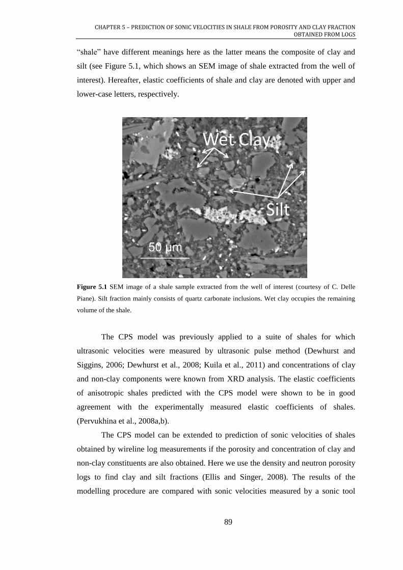
CHAPTER 5 – PREDICTION OF SONIC VELOCITIES IN SHALE FROM POROSITY AND CLAY FRACTION OBTAINED FROM LOGS
89
“shale” have different meanings here as the latter means the composite of clay and
silt (see Figure 5.1, which shows an SEM image of shale extracted from the well of
interest). Hereafter, elastic coefficients of shale and clay are denoted with upper and
lower-case letters, respectively.
Figure 5.1 SEM image of a shale sample extracted from the well of interest (courtesy of C. Delle
Piane). Silt fraction mainly consists of quartz carbonate inclusions. Wet clay occupies the remaining
volume of the shale.
The CPS model was previously applied to a suite of shales for which
ultrasonic velocities were measured by ultrasonic pulse method (Dewhurst and
Siggins, 2006; Dewhurst et al., 2008; Kuila et al., 2011) and concentrations of clay
and non-clay components were known from XRD analysis. The elastic coefficients
of anisotropic shales predicted with the CPS model were shown to be in good
agreement with the experimentally measured elastic coefficients of shales.
(Pervukhina et al., 2008a,b).
The CPS model can be extended to prediction of sonic velocities of shales
obtained by wireline log measurements if the porosity and concentration of clay and
non-clay constituents are also obtained. Here we use the density and neutron porosity
logs to find clay and silt fractions (Ellis and Singer, 2008). The results of the
modelling procedure are compared with sonic velocities measured by a sonic tool

CHAPTER 5 – PREDICTION OF SONIC VELOCITIES IN SHALE FROM POROSITY AND CLAY FRACTION OBTAINED FROM LOGS
90
(DSI) from the same well. The detailed modelling procedure is described below. At
each step, we underline all assumptions that we make.
1. At the first step we calculate porosity, , of rock from density log as follows:
wgbg (5.1)
Here b is bulk density,
g is the matrix density obtained from the dry
weight fractions of the composite minerals measured by the ECS tool and w
is the saturating fluid density (brine for this particular well).
Alternatively, the porosity can be estimated from neutron logs by
calibrating it with laboratory core measurements. However, one must be
careful as the standard laboratory porosity measurement procedures are not
well established for shale and might give systematically biased results. It is
generally known that mercury intrusion porosimetry (MIP) underestimates
porosity in shales. Another method of estimation of free water mass fraction
in shales is based on the comparison of preserved (saturated) shale density
with the density of the dry shale (obtained by keeping it in an oven at a
temperature of 105C for 24 hours). This method assumes that all water has
been evaporated from the sample; this assumption is questionable, especially
for low permeability shales. Hereafter we use the porosity calculated from the
bulk and grain density using equation (5.1).
2. Clay and silt fractions out of the solid phase, 0
cf and 0
sf , are then estimated
using a neutron-density cross-plot (e.g., Ellis and Singer, 2008). The
volumetric clay and silt fractions are then calculated as:
10
cc ff (5.2)
and
cs ff 1 (5.3)
3. The wet clay porosity, , is determined as a ratio of the volume of pores to
the total volume of the clay constituent:
cf (5.4)

CHAPTER 5 – PREDICTION OF SONIC VELOCITIES IN SHALE FROM POROSITY AND CLAY FRACTION OBTAINED FROM LOGS
91
The WCP is analogous to the clay packing density parameter (CPD)
introduced by Ulm and Abousleiman (2006), but we find WCP more
intuitive. CPD and WCP are connected by a simple relation 1CPD . By
introducing WCP parameter in such a way, we assume that all the porosity is
hosted between clay platelets and that the silt is non-porous. This assumption
is plausible as, for the well of interest, the silt mostly consists of quartz
inclusions and these microscopic quartz particles can be considered as non-
porous.
4. We here assume that both the shale and its clay constituent are transversely
isotropic with a vertical symmetry axis (VTI). This is a reasonable
approximation for shales that are not subject to vertical fractures or
anisotropic horizontal stress. Furthermore, based on a number of laboratory
experiments, Pervukhina et al. (2008a,b) showed that a linear dependency of
shale elastic coefficients on clay packing density is a reasonable first order
approximation for a wide range of wet clay porosities. The dependency of the
elastic coefficients, ijc , on WCP will then be linear as well:
5.00
ijij cc (5.5)
Here 0
ijc are elastic coefficients of hypothetical clay with 0 , which were
obtained from the linear regression coefficients and were shown to be equal
to 0
11c = 46.4 GPa, 0
33c = 29.9 GPa, 0
13c = 17.9 GPa, 0
44c = 6.7 GPa and
0
66c = 11.2 GPa (Pervukhina et al., 2008a). The coefficient 0.5 arises in
equation 5.5 as we assume that the wet clay is not load-bearing if the
volumetric water fraction in it is equal or exceeds 50%. Hereafter, we use
these relations to estimate elastic coefficients of clay based of porosities and
clay fractions obtained by logs (equations 5.1 and 5.2).
5. Steps 1-4 give allow us to compute anisotropic elastic moduli of wet clay. In
addition to wet clay, the shale usually contains significant amount of silt
inclusions, Indeed, the concept that silt fraction has a prominent effect on
elastic coefficients of shales and that this effect must be taken into account is
widely accepted (e.g., Hornby et al., 1994; Bayuk et al., 2007; Ulm and

CHAPTER 5 – PREDICTION OF SONIC VELOCITIES IN SHALE FROM POROSITY AND CLAY FRACTION OBTAINED FROM LOGS
92
Abousleiman, 2006). We take into account the effect of the silt inclusions
using an anisotropic Differential Effective Medium (DEM) approach
(Nishizawa, 1982). The DEM method calculates elastic properties of shale by
incrementally adding silt inclusions into the clay matrix up to the measured
fraction of the silt constituent (equation 5.2). Anisotropic elastic properties of
the clay matrix are calculated from equation 5.5. Application of DEM model
implies that silt is present in the form of isolated inclusions in the
interconnected clay matrix. The silt inclusions are modelled as quartz
spheroids. The assumption of connectivity of the clay matrix and round shape
of silt inclusions are consistent with observations of numerous SEM images
(e.g., Desbois, 2009). It is worth noting that this approach is not applicable to
shaly sands in which microstructural distribution of clay in a sandstone
should be taken into account and which can depend of clay fraction and
compaction (for more detailed information see, for instance, Sams and
Andrea, 2001).
6. Elastic wave velocities in the direction normal to bedding are then calculated
as follows:
21
33 bP CV (5.6)
21
44 bS CV (5.7)
These equations will give sonic velocities in a well that is drilled normal to
bedding plane. In the case of a deviated well or tilted bedding, the calculation
of the velocities from the elastic coefficients depends on whether group or
phase velocity is measured by a sonic tool. The detailed discussion on this
topic can be found in Miller et al. (2012) and Pervukhina et al. (2013).
7. To estimate uncertainties of the velocity simulation at each depth, we perform
simulations with N=100 realisations of the input parameters (namely,
porosity, , and clay fraction, fc, with added Gaussian noise of 5%). The
mean and standard deviation for both compressional and shear velocities are
then calculated as:

CHAPTER 5 – PREDICTION OF SONIC VELOCITIES IN SHALE FROM POROSITY AND CLAY FRACTION OBTAINED FROM LOGS
93
N
fV
V
N
i
i
c
i 1
,
(5.8)
and
1
1
2
N
VVN
i
i
(5.9)
5.3 LOG DATA EXAMPLE
To test the predictions of the workflow described above, we apply it to log
data in a vertical well. Log data, namely, gamma ray (GR), bulk and grain density,
neutron and density porosity and mineralogy measured in the well are shown in
Figure 5.2. The distance between the major grid lines is 100 metres and between the
minor ones is 25 metres.
The GR values are high (160-180 gAPI) throughout the whole 500 metres
depth interval apart from the interval of about 40 metres in the middle and a few
short intervals at the bottom. The high gamma ray values are a good indication of
shales if no other radioactive minerals are present. The abundance of the shale in the
well is also confirmed by the deviation of the measured neutron porosity from the
porosity calculated from density using equation 5.1. Neutron porosity is up to 20%
higher than density porosity in the depth intervals with high gamma ray readings and
the porosities match each other in the depth intervals with low gamma ray values.
Modelling of shale properties is done only for the depths at which silt fraction is
below 0.4.
Figure 5.3 gives a visual illustration that the silt effect on elastic properties of
shales is observable on the log measurement scale. The elastic coefficients of shales
are then plotted against wet clay porosity, , and colour coded in accordance with silt
fraction, fs. Elastic coefficients C33 are calculated from sonic velocities and bulk
density as follows:
2
33 PbVC (5.10)
2
44 SbVC (5.11)
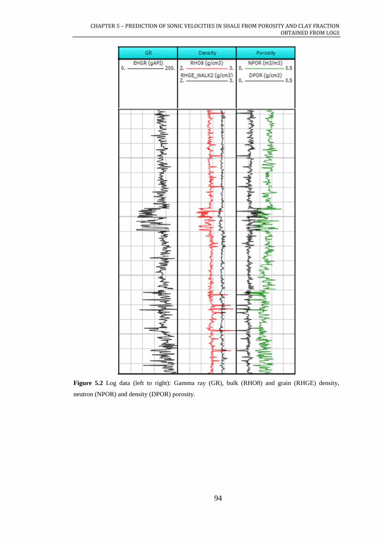
CHAPTER 5 – PREDICTION OF SONIC VELOCITIES IN SHALE FROM POROSITY AND CLAY FRACTION OBTAINED FROM LOGS
94
Figure 5.2 Log data (left to right): Gamma ray (GR), bulk (RHO8) and grain (RHGE) density,
neutron (NPOR) and density (DPOR) porosity.

CHAPTER 5 – PREDICTION OF SONIC VELOCITIES IN SHALE FROM POROSITY AND CLAY FRACTION OBTAINED FROM LOGS
95
Figure 5.3 Elastic coefficients C33 and C44 calculated from log data vs. wet clay porosity, , colour
coded with respect to silt fractions are compared to CPS model predictions for silt fractions of 0.4,
0.3, 0.2 and 0.1, which are shown by brown, yellow, cyan and blue, respectively.
The individual coefficients C33 and C44 are shown for shale ( 4.0sf )
throughout the whole depth interval. The same elastic coefficients simulated using
DEM approach for four different silt fractions 0.1, 0.2, 0.3 and 0.4 are shown by light
blue, green, orange and dark red solid lines, respectively. The elastic coefficients of
shale regardless its silt fraction exhibit significant scatter and show no obvious trend
with wet clay porosity. However, for a narrower range of silt fractions, for example,
from 0.1 to 0.2, the elastic coefficients show obvious trends that are similar to the
trends of model predictions.
Gamma ray log, measured sonic velocities and CPS model predictions are
shown in Figure 5.4 at two different scales. In Figure 5.4a the sonic velocities (blue
lines) are shown in comparison with mean modelled velocities (red lines) calculated
using equation (5.8) throughout the whole shale interval of about 500 metres. The
dashed and dotted lines are the smoothed measured sonic velocities plus and minus
10%, respectively. In Figure 5.4b the gamma ray and velocities are shown for a ~50
metre interval. Red dashed and dotted lines in Figure 5.4b are 2V , where mean
velocities and standard deviation are calculated using equations (5.8) and (5.9).
0 0.1 0.2 0.3 0.4 0.50
5
10
15
20
25
30
35
40
45
C33 &
C44, G
Pa
Silt
fra
ctio
n
0.1
0.15
0.2
0.25
0.3
0.35
0.4
C33
C44

CHAPTER 5 – PREDICTION OF SONIC VELOCITIES IN SHALE FROM POROSITY AND CLAY FRACTION OBTAINED FROM LOGS
96
(a) (b)
Figure 5.4 Gamma ray, compressional and shear sonic velocities (blue lines) in comparison with
simulated velocities (red lines): (a) throughout the whole shale interval, the depth between major
gridlines is 100 m; (b) throughout about 50 m of depth; 10 m distance between gridlines.
The cross-plot of the modelled versus measured velocities is shown in Figure
5.5. The modelled compressional velocity is in a good agreement with measured
sonic log velocity with linear regression coefficient of 1.0 and the coefficient of
determination R2=0.8. The modelled shear velocities show a systematic shift of about
8% but the coefficient of determination is still 0.8. This discrepancy might be
explained by the fact that for the forward modelling we used the elastic coefficients
of clay that were derived from laboratory experiments on preserved shale samples
excavated from different places all over the world (details can be found in
Pervukhina et al., 2008a,b). In the following sections, we invert the log sonic
velocities measured in shales for elastic coefficients of clay but we do not use these
coefficients for forward modelling. The purpose of the inversion is to study
variations of clay properties with wet clay porosity and with depth in more detail,
rather than to fit modelling results with the measured ones.

CHAPTER 5 – PREDICTION OF SONIC VELOCITIES IN SHALE FROM POROSITY AND CLAY FRACTION OBTAINED FROM LOGS
97
Figure 5.5 Modelled shale velocities vs. measured sonic log velocities.
5.4 INVERSION FOR ELASTIC PROPERTIES OF WET CLAY
In the previous section, we showed that the CPS model can be used to
estimate elastic moduli of shales from porosity and mineralogy logs. In the interval
covered by sonic data, we can also invert the sonic velocity and silt fraction for
elastic moduli of wet clay using the anisotropic DEM model without a priori
knowledge of the relationship between clay moduli and porosity. However, it is
worth noting that the inversion is limited to two elastic coefficients of clays 33c and
44c , as only these elastic coefficients of shale can be obtained from sonic velocity
measurements in vertical wells drilled normal to bedding.
Here we invert the elastic properties of shales obtained from the sonic log
measurements in the same vertical well throughout the whole 500 metres shale
interval. The inversion is done by minimising the function:
4
3
2exp,,,i
iiiis
DEM
iiii CcfCc (5.12)
Elastic coefficients of shales exp
iiC are calculated from sonic log velocities
using equations (5.10) and (5.11). DEM
iiC are simulated using anisotropic DEM
(Nishizawa, 1982). and fs are calculated for a particular depth log measurements
using equations (5.3) and (5.4). The inversion is done for several aspect ratios, α, of

CHAPTER 5 – PREDICTION OF SONIC VELOCITIES IN SHALE FROM POROSITY AND CLAY FRACTION OBTAINED FROM LOGS
98
silt inclusion ranging from 0.1 to 1. The initial guess for the inversion is obtained
using equation (5.5) with 0
33c = 29.9 GPa, and 0
44c = 6.7 GPa. The Levenberg-
Marquardt method (Moré, 1977) implemented in the MATLAB optimization toolbox
is used to minimise function (5.12).
To study sensitivity of the inverted elastic coefficients of clay to the aspect
ratio of silt inclusions, we inverted 33C and 44C for elastic coefficients of clays for
six aspect ratios of silt inclusions of 0.1, 0.2, 0.3, 0.5, 0.7 and 1.0. The study is
limited to the aspect ratios in the range from 0.1 to 1.0 as these aspect ratios of the
silt inclusions have been observed in micro- and nanotomographic studies of shale
microstructure. The inverted 33C and 44C are plotted in Figure 5.6 against for silt
inclusion aspect ratio of 1. This figure demonstrates that removing the effect of silt
dramatically reduced the large scatter (as shown in Figure 5.3) of the elastic moduli
for a given clay porosity. Elastic coefficients exhibit obvious negative trend with the
increase of WCP. The best fit linear trends are shown in the same plot by black solid
lines. Elastic coefficients 0
33c and 0
44c of the clay in the hypothetic non-porous state
(with zero wet clay porosity) can be obtained by extrapolating the trend lines to zero
WCP.
Figure 5.6 Elastic coefficients, c33 and c44, of clay obtained by the inversion procedure against wet
clay porosity using silt aspect ratio of 1 (i.e. spherical). The best linear fit is shown by black line.
0
5
10
15
20
25
30
35
0 0.05 0.1 0.15 0.2 0.25 0.3
c33
&
c4
4, G
Pa
c33
c44

CHAPTER 5 – PREDICTION OF SONIC VELOCITIES IN SHALE FROM POROSITY AND CLAY FRACTION OBTAINED FROM LOGS
99
The elastic coefficients at zero wet clay porosity are shown in Table 5.1 for
different aspect ratios of silt inclusions of 0.1, 0.2, 0.3, 0.5, 0.7 and 1.0. The averaged
values are 3.03.320
33 c and .1.05.70
44 c One can see that the effect of the
aspect ratio of silt inclusions on the inverted coefficients of clays does not exceed
2%. This indicates that the rigorous bounds for elastic moduli are quite close for
these moduli of the constituents. Therefore, in further analysis, we use elastic
coefficients inverted using silt particles with aspect ratios of 1.0 (i.e., spheres). These
values of the elastic coefficients of hypothetic clay with zero porosity are close
(especially for c33) to the values of 29.9 GPa and 6.7 GPa, which were acquired from
laboratory measurements (Pervukhina et al., 2008a) and are used for forward
modelling.
Table 5.1 Results the linear extrapolation of the inverted clay coefficients to 0 using silt
inclusions with different aspect ratios, α. Coefficients of determination, R2, indicate that linear trends
fit the inverted coefficients better in the cases of large aspect ratios of silt inclusions.
α 0.1 0.2 0.3 0.5 0.7 1.0
33c , GPa 32.0 32.0 32.1 32.3 32.4 32.7
2
33R 0.7 0.7 0.7 0.8 0.8 0.8
44c , GPa 7.3 7.4 7.5 7.6 7.6 7.6
2
44R 0.5 0.6 0.7 0.7 0.7 0.7

CHAPTER 5 – PREDICTION OF SONIC VELOCITIES IN SHALE FROM POROSITY AND CLAY FRACTION OBTAINED FROM LOGS
100
5.5 DISCUSSION
The inversion results for the moduli c33 and c44 of clay, corresponding to the
original moduli of shale C33 and C44, wet clay porosity and silt fraction are shown in
Figure 5.7 (a, b). The best linear fits of these values are shown in the same plots and
Table 5.2 summarises their depth gradients. We see that the shale moduli, C33 and
C44, systematically increase with depth by ~5% and ~3% per 100 metres,
respectively. Assuming that wet clay porosity decreases with depth due to
compaction, we must expect to see some increase of clay elastic coefficients with
depth. As a matter of fact for this particular well, the depth gradients of either WCP
or clay elastic coefficients c33 and c44 are negligible (Table 5.2). Instead, a noticeable
silt fraction increase with the increase of depth of 4% per 100 metres is detected,
which may explain the observed stiffening of the shale.
The lack of increase of compaction-induced porous clay moduli with depth is
intriguing. This might be the result of the fact that the clay fraction is obtained from
the neutron-density separation using a single clay point for the whole 500 metres
depth. It is hard to assess the validity
of this assumption in our well since
it shows very large systematic
increase of silt fraction with depth. It
is most likely that the depth interval
of 500 metres is simply not
sufficient to clearly see the
compaction trend and separate it
from the strong shale trend caused
by the changes in silt and clay
fractions. This issue requires further
analysis.
Table 5.2 Depth gradients.
Per 100 meters
33C,GPa 5%
44C, GPa 3%
33c, GPa -0.5%
44c, GPa -0.5%
, % -0.5%
sf, % 4%

CHAPTER 5 – PREDICTION OF SONIC VELOCITIES IN SHALE FROM POROSITY AND CLAY FRACTION OBTAINED FROM LOGS
101
(a) (b)
Figure 5.7 Depth dependencies of elastic coefficients, silt fraction and wet clay porosity: (a) C33
(green), c33 (blue), C44 (red) and c44 (magenta) and (b) wet clay porosity (red) and silt fraction (blue).
By depth here, we mean the depth from some non-zero level.
0 10 20 30 40
0
100
200
300
400
500
Elastic moduli, GPa
Depth, m
0 0.1 0.2 0.3 0.4 0.5
0
100
200
300
400
500
Silt fraction and wet clay porosity
Depth, m

CHAPTER 5 – PREDICTION OF SONIC VELOCITIES IN SHALE FROM POROSITY AND CLAY FRACTION OBTAINED FROM LOGS
102
5.6 CHAPTER CONCLUSIONS
We have confirmed that wet clay porosity and silt fraction are the two key
parameters for modelling of elastic properties of shales. These parameters can be
obtained from clay fraction derived from common well log measurements such as
neutron-density separation or similar quantitative mineralogy information.
Knowledge of these parameters allowed prediction of elastic properties of shales
throughout the depth interval of about 500 metres without detailed knowledge of the
shale mineralogy. The predicted velocities show good agreement with the measured
velocities but a systematic shift is observed for shear velocities.
The analysis of the elastic properties of clay inverted on the basis of the
knowledge of the log measurements of sonic velocities, bulk and grain density, plus
silt fraction shows that in the considered well, the increase in elastic coefficients of
shales is controlled by the increase of silt fraction with depth. Elastic coefficients of
clay show no increase with depth. Furthermore, compared to the elastic moduli of
shale, the inverted elastic moduli of wet clay show much stronger correlation with
clay porosity, which confirms the hypothesis that silt fraction is one of the key
parameters for modelling of elastic properties of shale.

CONCLUDING REMARKS
103
CONCLUDING REMARKS
Various research aspects covered in this thesis include (a) 3D reconstruction
of X-ray microtomographic images for acquisition of realistic computer models of
rocks, (b) experimental verification of velocity-stress relationship for isotropic
porous rocks, (c) shale anisotropy and parameterization of elastic stress sensitivity in
shales, (d) prediction of sonic velocities in shales from clay and silt fractions from
the data obtained from wire logging tools without detailed knowledge of rock
mineralogy. Given the diversity of petrophysics problems addressed in this thesis and
independence of some chapters, obtained results from each chapter are summarised
individually:
Chapter 1. A comprehensive digital rock physics workflow has been
developed to support realistic 3D image reconstruction, processing and noise
suppression, and finite element method simulations to complement laboratory
experiments. On a computer model reconstructed from a real sandstone
specimen it has been demonstrated that numerically simulated elastic moduli
correlate well with laboratory measurements, proving the method
applicability for computational up-scaling of elastic moduli of porous rocks.
Chapter 2. Dual porosity concept and its interpretation of exponential stress
dependency of elastic properties of rocks has been tested using laboratory
measurements on dry sandstones and has shown that (a) elastic
compressibility is linearly dependant on soft porosity, and (b) exponential
decay of soft porosity and elastic compressibility can be observed with
effective stress up to 60 MPa. The obtained results reconfirm the applicability
of Shapiro’s (2003) stress sensitivity model and hence provide justification
for using this approach to model the effect of stress on properties of both
isotropic and anisotropic rocks.
Chapter 3. The main objective has been achieved with the development of a
new stress dependency model for TI media for parameterization of
dependencies of the elastic properties of shales. The proposed model is based
on a combination of the dual porosity approach of Shapiro (2003) and the
CONCLUDING REMARKS
104
non-interactive approximation of Sayers and Kachanov (1995). Our findings
suggested that the proposed model allows the prediction of stress dependency
of all five elastic compliances if only three or four compliances are known.
This opens up new opportunities for the reconstruction of stress dependencies
of all five elastic compliances of shale from log data, when detailed
information is not available or is hard to obtain.
Chapter 4. In this chapter, we further developed the model proposed in
Chapter 3 for prediction of elastic properties variation due to application of
uniaxial stress for TI media with discontinuities. The results of numerical
simulations have shown that (a) effects caused by application of small
uniaxial stresses can be described using four physically plausible parameters,
and (b) predicted variations in elastic velocities are in a good agreement with
experimentally measured data. This allowed the model to be used for
prediction of elastic properties response to application of a small uniaxial
stress normal to the bedding plane when only variation of elastic properties
with isotropic stress is known.
Chapter 5. In this chapter, we used the Clay-Plus-Silt (CPS) model that is
based on two physical parameters, namely, clay packing density and silt
fraction that are considered to be the key parameters for modelling of elastic
properties of shales. Knowledge of these parameters allows accurate
prediction of elastic properties of shales without detailed mineralogical
analysis, whereas clay packing density and silt fraction parameters may
relatively easy be obtained from wireline measurements or derived from
common log measurements such as neutron-density separation or similar
quantitative mineralogy information. The clay packing density parameter is
shown to be a proxy of the effect of compaction processes on elastic
properties of clay matrix of shales. Elastic coefficients of clay have shown no
increase with depth. The predicted velocities show good agreement with the
measured velocities but a systematic shift is observed for shear velocities. In
addition, the inverted elastic moduli of wet clay, as compared to the elastic
moduli of shale, have shown much stronger correlation with clay porosity.

CONCLUDING REMARKS
105
This confirmed the hypothesis that silt fraction is one of the key parameters
for modelling of elastic properties of shale.

REFERENCES
106
REFERENCES
ABAQUS, Inc., 2004, ABAQUSTM, ABAQUS. Version 6.5 Documentation.
Abousleiman, Y., Tran, M. H., Hoang, S. K., Ortega, J. A. and Ulm, F. J., 2010,
Geomechanics field characterization of Woodford Shale and Barnett Shale
with advanced logging tools and nano-indentation on drill cuttings. The
Leading Edge, 29, 730-736.
Aleksandrov, K. S. and Ryzhova, T. V., 1961, Elastic properties of rock-forming
minerals II. Layered silicates, Bull. Acad. Sci. USSR, Geophys. Ser. English
translation (12), 1165-1168.
Alliez, P., Ucelli, G., Gotsman, C. and Attene, M., 2005, Recent Advances in
Remeshing of Surfaces. Research Report, AIM@SHAPE Network of
Excellence.
Al-Raoush, R. I. and Wilson, C. S., 2005, A pore-scale investigation of a multiphase
porous media system. Journal of Contaminant Hydrology, 77 (2005), 67 – 89,
doi:10.1016/j.jconhyd.2004.12.001.
Angus, D. A., Verdon, J. P., Fisher, Q. J. and Kendall, J. M., 2009, Exploring trends
in microcrack properties of sedimentary rocks: An audit of dry-core velocity-
stress measurements. Geophysics, 74(5), E193-E203.
Arns, C. H., Knackstedt, M. A., Pinczewski, W. V. and Garboczi, E. J., 2002,
Computation of linear elastic properties from microtomographic images:
Methodology and agreement between theory and experiment. Geophysics,
67(5), 1396-1405.
AVIZO, VSG. (2009). Visilog 6, reference guide.
Avseth, P., Draege, A., A.-J. Van Wijngaarden, Johansen, T. A. and Jorstad, A.,
2008, Shale rock physics and implications for AVO analysis: A North Sea
demonstration. The Leading Edge, 27(6), 788-797.
Banik, N. C., 1984, Velocity anisotropy in shales and depth estimation in the North
Sea basin. Geophysics, 49, 1411-1419.
Barber, C. B., Dobkin, D. P. and Huhdanpaa, H. T., 1996, The Quickhull Algorithm
for Convex Hulls. ACM Trans. Mathematical Software, 22, 469-483.
Bayuk, I. O., Ammerman, M. and Chesnokov, E. M., 2007, Elastic moduli of
anisotropic clay. Geophysics, 72(5), D107-D117.

REFERENCES
107
Becker, K., Shapiro, S., Stanchits, S., Dresen, G. and Vinciguerra, S., 2007, Stress
induced elastic anisotropy of the Etnean basalt: Theoretical and laboratory
examination. Geophysical Research Letters, 34(11).
Berryman, J. G., 1980. Long-wavelength propagation in composite elastic media I.
Journal of Acoustic Society of America, 69, 416-424.
Berryman, J. G., 1980. Long-wavelength propagation in composite elastic media II.
Ellipsoidal inclusions. Journal of Acoustic Society of America, 68(6), 1820-
1831.
Castagna, J. P., Batzle, M. L. and Eastwood, R. L., 1985, Relationships between
Compressional-Wave and Shear-Wave Velocities in Clastic Silicate Rocks,
Geophysics, 50(4), 571-581.
Castagna, J. P., Batzle, M. L. and Kan T. K., 1993, Rock physics – The link between
rock properties and AVO response in Offset-Dependent Reflectivity in Theory
and practice of AVO Analysis, edited by Castagna, J. P. and Backus, M., pp.
135-171, Society of Exploration Geophysicists, Tulsa, Oklahoma.
Ciz, R. and Shapiro, S. A., 2009, Stress-dependent anisotropy in transversely
isotropic rocks: Comparison between theory and laboratory experiment on
shale. Geophysics, 74(1), D7-D12.
Crampin, S., 1985, Evaluation of anisotropy by shear‐wave splitting. Geophysics,
50(1), p. 142-152, doi: 10.1190/1.1441824.
De Berg, M., Cheong, O., Kreveld, M. and Overmars, M., 2008, Computational
Geometry: Algorithms and applications. Springler-Verlag. ISBN 978-3-540-
77973-5.
De Paula, O. B., Pervukhina, M. and Gurevich, B., 2008, Role of compliant porosity
in stress dependency of ultrasonic velocities in carbonates and sandstones.
Proceedings of the third National Geophysical symposium, Belem-Para.
Delaunay, B., 1934, Sur la Sphere Vide. Izvestia Akademia Nauk SSSR, VII Seria,
Otdelenie Matematicheskii i Estestvennykh Nauk, 7, 793-800.
Delle Piane, C., Dewhurst, D. N., Siggins, A. F. and Raven, M. D., 2010, Stress-
induced anisotropy in saturated shale. Geophysical Journal International,
184(2), 897-906, doi:10.1111/j.1365-246X.2010.04885.x.

REFERENCES
108
Desbois, G., Urai, J. L. and Kukla, P. A., 2009, Morphology of the pore space in
claystones – evidence from BIB/FIB ion beam sectioning and cryo-SEM
observations, eEarth, 4, 15-22.
Dewhurst, D. N. and Siggins, A. F., 2006, Impact of fabric, misrocracks and stress
field on shale anisotropy, Geophysical Journal International, 165, 135-148.
Dewhurst, D. N., Siggins, A. F., Kuila, U., Clennell, M. B., Raven, M. D. and
Nordgard-Bolas, H. M., 2008a, Elastic, Geomechanical and Petrophysical
Properties of Shales. Paper presented at American Rock Mechanics
Association Symposium.
Dewhurst, D. N., Siggins, A. F., Kuila, U., Clennell, M. B., Raven, M. D. and
Nordgard-Bolas, H. M., 2008b, Rock Physics, Geomechanics and Rock
Properties in Shales: Where Are The Links?, Paper presented at Proceedings of
the 1st SHIRMS conference.
Draege, A., Jakobsen, M. and Johansen, T. A., 2006, Rock physics modelling of
shale diagenesis. Petroleum Geoscience, 12(1), 49-57.
Drury, M. R. and Fitz Gerald, J. D., 1996, Grain boundary melt films in an
experimentally deformed olivine-orthopyroxene rock: implications for melt
distribution in upper mantle rocks. Geophysical Research Letters, 23, 701–704.
Dvorkin, J., 2009, Accuracy and Relevance of Digital Rock Results: Successes and
Failures. Ingrain Digital Rock Physics Lab, 1-22.
Eberhart-Phillips, D., Han, D.-H. and Zoback, M. D., 1989, Empirical relationships
among seismic velocity, effective pressure, porosity and clay content in
sandstone. Geophysics, 54(1), 82-89.
Ellis, D. V. and Singer, J. M., 2008, Well Logging for Earth Scientists. Springer, The
Netherlands.
Flannery, B. P., Deckman, H. W., Roberge, W. G. and D'Amico, K. L., 1987, Three-
Dimensional X-ray Microtomography. Science, 237(4821), 1439-1444.
Fortin, J., Gueguen, Y. and Schubnel, A., 2007, Effects of pore collapse and grain
crushing on ultrasonic velocities and Vp/Vs. Journal of Geophysical Research,
112, B08207, doi:10.1029/2005JB004005.
Garbozci, E. J., 1998, Finite element and finite difference programs for computing
the linear electrical and elastic properties of digital images of random
materials. National Institute of Standards and Technology Internal report.

REFERENCES
109
Garland, M. and Heckbert, P., 1997, Surface simplification using quadric error
metrics. Proceedings of the 24th Annual Conference on Computer Graphics
and Inteactive Techniques, 209-216.
Gassmann, F., 1951, Uber die Elastizitat poroser Medien. Vierteljahrschrift der
Naturforschenden Gesellschaft in Zurich, 96, 1-23.
Gurevich, B., Makarynska, D. and Pervukhina, M., 2009, Are penny-shaped cracks a
good model for compliant porosity? SEG, edited. SEG, Houston, USA.
Gurevich, B., Makarynska, D., Pervukhina, M. and De Paula, O., 2009, A New
Squirt-Flow Model for Elastic Wave Attenuation and Dispersion in Fluid-
Saturated Rocks. Poro-Mechanics Iv, 700-705, 1151.
Gurevich, B., Pervukhina, M. and Makarynska, D., 2011, An analytical model for
stress-induced anisotropy of dry rocks. Geophysics, 76, 125-133.
Han, D.-H., Nur, A. and Morgan, D., 1986, Effects of porosity and clay content on
wave velocities in sandstones. Geophysics, 51, 2093-2107.
Hornby, B. E., Schwartz, L. M. and Hudson, J. A., 1994, Anisotropic effective-
medium modeling of the elastic properties of shales. Geophysics, 59(10), 1570-
1583.
Hornby, B. E., 1998, Experimental laboratory determination of the dynamic elastic
properties of wet, drained shales. Journal of Geophysical Research, 103,
29945–29964.
Jakobsen, M. and Johansen, T. A., 2000, Anisotropic approximations for mudrocks:
a seismic laboratory study. Geophysics, 65, 1711-1725.
Jakobsen, M., Hudson, J. A., Minshull, T. A. and Singh, S. C., 2000, Elastic
properties of hydrate-bearing sediments using effective medium theory. Journal
of Geophysical Research - Solid Earth, 105(B1), 561-577.
Jensen, E. H., Andersen, C. F. and Johansen, T. A., 2011, Estimation of elastic
moduli of mixed porous clay composites. Geophysics, 76, E9-E20.
Johansen, T. A., Ruud, B. O. and Jakobsen, M., 2004, Effect of grain scale alignment
on seismic anisotropy and reflectivity of shales. Geophysical Prospecting, 52,
133-149.
Johnston, J. E. and Christensen, N. I., 1993, Compressional to shear velocity ratios in
sedimentary rocks: International Journal of Rock Mechanics and Mining
Sciences and Geomechanics. Abstract, 30, 751-754.

REFERENCES
110
Johnston, J. E. and Christensen, N. I., 1995, Seismic anisotropy of shales. Journal of
Geophysical Research, 100(B4), 5991-6003.
Jones, L. E. A. and Wang, H. F., 1981, Ultrasonic Velocities in Cretaceous Shales
from the Williston Basin. Geophysics, 46(3), 288-297.
Kachanov, M., Prioul, R. and Jocker, J., 2010, Incremental linear-elastic response of
rocks containing multiple rough fractures: Similarities and differences with
traction-free cracks. Geophysics, 75(1), D1-D11.
Kaestner, A., Lehmann, E. and Stampanoni, M., 2008, Imaging and image
processing in porous media research. Advances in Water Resorces, 31, 1174-
1187.
Katahara, K. W., 1996, Clay mineral elastic properties, in SEG Annual Meeting
Expanded Technical Programme Abstracts, edited, pp. 1691-1694.
Kuila, U., Dewhurst, D. N., Siggins, A. F. and Raven, M. D., 2011, Stress anisotropy
and velocity anisotropy in low porosity shale. Tectonophysics,
doi:10.1016/j.tecto.2010.09.023, 503(1-2), 34-44.
Liu, H. H., Rutqvist, J. and Berryman, J. G., 2008, On the relationship between stress
and elastic strain for porous and fractured rock. International Journal of Rock
Mechanics and Mining Sciences, 46(2), 289-296,
doi:10.1016/j.ijrmms.2008.04.005.
MacBeth, C., 2004, A classification for the pressure-sensitivity properties of a
sandstone rock frame. Geophysics, 69, 497-510.
MacBeth, C. and Schuett, H., 2007, The stress dependent elastic properties of
thermally induced microfractures in aeolian Rotliegend sandstone. Geophysical
Prospecting, 55(3), 323-332.
Marion, D. and Nur, A., 1991, Pore-Filling Material and Its Effect on Velocity in
Rocks. Geophysics, 56(2), 225-230.
Marion, D., 1990, Acoustical, mechanical and transport properties of sediments and
granular materials. Stanford University.
Matthijs de Winter, D. A., Schneidjdenberg, C. T. W. M., Lebbink, M. N., Lich, B.,
Verkleij, A. J., Drury, M. R. and Humbel, B. M., 2009, Tomography of
insulated biological and geological materials using focused ion beam (FIB)
sectioning and low-kV BSE imaging. Journal of Microscopy, 233, 372–383.
REFERENCES
111
Mavko, G. and Nur, A., 1978, The effect of Nonelloptical Cracks on the
Compressibility of Rocks, Journal of Geophysical Research, 83, 4459-4468,
1978.
Mavko, G., and Jizba, D., 1991, Estimating grain-scale fluid effects on velocity
dispersion in rocks. Geophysics, 56(12), 1940-1949.
Mavko, G., Mukerji, T. and Dvorkin, J., 1998, The rock physics handbook. Tools for
seismic analysis in porous media. Cambridge University Press. ISBN 0 521
62068 6.
Mayo, S., Davis, T., Gureev, T., Miller, P., Paganin, D., Pogany, A., Stevenson, A.
and Wilkins, S., 2003, X-ray phase-contrast microscopy and microtomography.
Optic Express, 11(19), 2289-2302.
Miller, D. E., Horne, S. A. and Walsh, J., 2012, Precise inversion of logged
slownesses for elastic parameters in a gas shale formation. Geophysics, 77(4),
B197-B206.
Mondol, N. H., Bjorlykke, K., Jahren, J. and Hoeg, K., 2007, Experimental
mechanical compaction of clay mineral aggregates - Changes in physical
properties of mudstones during burial. Marine and Petroleum Geology, 24,
289-311.
Moré, J. J., 1977, The Levenberg-Marquardt Algorithm: Implementation and Theory.
Springer Verlag.
Najman, L. and Schmitt, M., 1994, Watershed of a continuous function. Signal
Processing (Special issue on Mathematical Morphology), 38, 99–112.
Nikolaou, N. and Papamarkos, N., 2009, Color reduction for complex document
images. International Journal of Imaging Systems and Technology, 19(1), 14-
26.
Nishizawa, O., 1982, Seismic velocity anisotropy in a medium containing oriented
cracks - transversely isotropic case. Journal of Physics of the Earth, 30, 331-
347.
Nur, A., 1971, Effects of stress on velocity anisotropy in rocks with cracks. J.
Geophys. Res., 76, 2022-2034.
Nygard, R., Gutierrez, M., Gautam, R. and Hoeg, K., 2004, Compaction behavior of
argillaceous sediments as function of diagenesis. Marine and Petroleum
Geology, 21, 349–362.

REFERENCES
112
Ortega, J. A., Ulm, F.-J. and Abousleiman, Y., 2007, The effect of the nanogranular
nature of shale on their poroelastic behavior. Acta Geotechnica.
Ortega, J. A., Ulm, F. J. and Abousleiman, Y., 2009, The nanogranular acoustic
signature of shale. Geophysics, 74(3), D65-D84.
Pal-Bathija, A., Prasad, M., Liang, H., Upmanyu, M., Lu, N. and Batzle, M., 2008,
Elastic properties of clay minerals. SEG Technical Program Expanded
Abstracts 2, edited, pp. pp. 1610-1614.
Peltonen, C., Marcussen, O., Bjorlykke, K. and Jahren, J., 2008, Mineralogical
control on mudstone compaction: a study of Late Cretaceous to Early Tertiary
mudstones of the Voring and More basins, Norwegian Sea. Petroleum
Geoscience, 14, 127-138.
Peltonen, C., Marcussen, O., Bjorlykke, K. and Jahren, J., 2009, Clay mineral
diagenesis and quartz cementation in mudstones: the effects of the smectite to
illite reaction on rock properties. Marine and Petroleum Geology, 26, 887-898.
Pervukhina, M., Siggins, A. F., Dewhurst, D. N. and Gurevich, B., 2007, Elastic
properties of shales with respect to silt fraction. ASEG, Extended Abstract,
Perth.
Pervukhina, M., Dewhurst, D. N., Gurevich, B., Kuila, U., Siggins, A. F., Raven, M.
and Hordgard Bolas, H. M., 2008a, Stress-dependent elastic properties of
shales: Measurement and modeling. The Leading Edge, 27(6), 772-779.
Pervukhina, M., Dewhurst, D. N., Kuila, U., Siggins, A. F. and Gurevich, B., 2008b,
Stress Dependent Anisotropy in Shales: Measurements and Modelling.
Proceedings. SHIRMS, 2, 287-300.
Pervukhina, M., Gurevich, B., Dewhurst, D. N. and Siggins, A. F., 2010,
Applicability of velocity–stress relationships based on the dual porosity
concept to isotropic porous rocks. Geophysical Journal International, 181(3),
1473–1479, doi:10.1111/j.1365-246X.2010.04535.x.
Pervukhina, M., Delle Piane, C., Dewhurst, D. N., Clennell, M. B. and Nordgard
Bolas, H. M., 2013, An Estimation of Pore Pressure in Shales from Sonic
Velocities. 83rd SEG Annual Meeting, Extended Abstract, Houston, USA.
Prasad, M., Kopycinska, M., Rabe, U. and Arnold, W., 2002, Measurement of
Young's modulus of clay minerals using atomic force acoustic microscopy.
Geophysical Research Letters, 29(8).
REFERENCES
113
Prasad, M., Hofmann, R., Batzle, M., Kopycinska-Muller, M., Rabe, U. and Arnold,
W., 2005, Values of mineral modulus of clay. SEG Technical Program
Expanded Abstracts.
Prioul, R. and Lebrat, T., 2004, Calibration of velocity-stress relationships under
hydrostatic stress for their use under non-hydrostatic stress conditions. SEG
Extended Abstract, edited, pp. 1698-1701, Denver, USA.
Prioul, R., Bakulin, A. and Bakulin, V., 2004, Nonlinear rock physics model for
estimation of 3D subsurface stress in anisotropic formations: Theory and
laboratory verification. Geophysics, 69(2), 415-425.
Qi, Z., Zambelli, J., Bevins, N. and Chen, G-H., 2010, Quantitative imaging of
electron density and effective atomic number using phase contrast CT. Physics
in Medicine and Biology, 55, 2669-2677.
Roberts, A. P. and Garboczi, E. J., 2000, Elastic properties of model porous
ceramics. Journal of American Ceramic Society, 83, 3041–3048.
Ruud, B. O., Jakobsen, M. and Johansen, T. A., 2003, Seismic properties of shales
during compaction. SEG Extended Abstract, Dallas, USA.
Saenger, E., Ciz, R., Kruger, O., Schmalholz, S., Gurevich, B. and Shapiro, S., 2007,
Finite-difference modelling of wave propagation on microscale: A snapshot of
the work in progress. Geophysics, 72(5), 1293-1300.
Sayers, C. M., 1988, Stress-induced ultrasonic wave velocity anisotropy in fractured
rock. Ultrasonics, 26, 311-317.
Sayers, C.M., 1988, Inversion of ultrasonic wave velocity measurements to obtain
the microcrack orientation distribution function in rocks. Ultrasonics, 26, 73-
77.
Sayers, C. and Kachanov, M., 1995, Microcrack-indused elastic wave anisotropy of
brittle rock. Journal of Geophysical Research, 100, 4149-4156.
Sayers, C., 1999, Stress-dependent seismic anisotropy of shales. Geophysics, 64(1),
93-98.
Sayers, C. and Han, D.-H., 2002, The effect of pore fluid on the stress-dependent
elastic wave velocities in sandstones. SEG Extended Abstract, Salt Lake City,
USA.
Sayers, C., 2005, Seismic anisotropy of shales. Geophysical Prospecting, 53, 667-
676.

REFERENCES
114
Sayers, C., Taleghani, A. D. and Adachi, J., 2009, The effect of mineralization on the
ratio of normal to tangential compliance of fractures. Geophysical Prospecting,
57(3), 439-446.
Sayers, C. M., 2013, The effect of anisotropy on the Young's moduli and Poisson's
ratios of shales. Geophysical Prospecting, 61(2), 416-426.
Schoenberg, M., 2002, Time-dependent anisotropy induced by pore pressure
variation in fractured rock. Journal of Seismic Exploration, 11(1-2), 83-105.
Shapiro, S. A., 2003, Elastic piezosensitivity of porous and fractured rocks.
Geophysics, 68(2), 482-486.
Shapiro, S. A. and Kaselow, A., 2005, Porosity and elastic anisotropy of rocks under
tectonic stress and pore-pressure changes. Geophysics, 70(5), 27-38.
Shikhaliev, P. M., 2008, Computed tomography with energy-resolved detection: a
feasibility study. Physics in Medicine and Biology, 53, 1475-1495.
Shulakova, V., Pervukhina, M., Lebedev, M., Mueller, T., Mayo, S., Schmid, S.,
Clennel, B. and Gurevich, B., 2011, Computation of elastic properties based on
microtomogram images. 73rd EAGE conference, Vienna, Austria, Extended
Abstract.
Siggins, A. F. and Dewhurst, D. N., 2003, Saturation, pore pressure and effective
stress from sandstone acoustic properties. Geophysical Research Letters, 30(2),
1089, doi:10.1029/2002GL016143.
Sinha, B. K., Vissapragada, B., Renlie, L. and Tysse, S., 2006, Radial profiling of the
three formation shear moduli and its application to well completions.
Geophysics, 71(6), E65-E77.
Solymar, M. and Fabricius, I. L., 1999, Image Analysis and Estimation of Porosity
and Permeability of Arnager Greensand, Upper Cretaceous, Denmark. Physics
and Chemistry of the Earth (A), 24(7), 587-591.
Spanne, P., Thovert, J., Jacquin, J., Lindquist, W. B., Jones, K. and Coker, D., 1994,
Synchrotron computed microtomography of porous media: topology and
transports. Physical Review Letters, 73, 2001-2004.
Storvoll, V. and Brevik, I., 2008, Identifying time, temperature, and mineralogical
effects on chemical compaction in shales by rock physics relations. The
Leading Edge, 27(6), 750-756, doi:10.1190/1.2944160.

REFERENCES
115
Surazhsky, V., Alliez, P. and Gotsman, C., 2003, Isotropic remeshing of surfaces: a
local parameterization approach. Proceedings of 12th International Meshing
Roundtable, Sandia National Laboratories, 215–224.
Szymczak, A., Rossignac, J. and King, D., 2003, Piecewise regular meshes:
Construction and compression. Graphical models.
Thomsen, L., 1986, Weak Elastic Anisotropy. Geophysics, 51(10), 1954-1966.
Tsvankin, I., 1997, Anisotropic parameters and P-wave velocities for orthorhombic
media. Geophysics, 62, 1292-1309.
Tsvankin, I., Larner, K., Gaiser, J. and Grechka, V., 2009, Seismic Anisotropy -
Introduction. Geophysics, 74(5), Wb1-Wb2.
Ulm, F. J. and Abousleiman, Y., 2006, The nanogranular nature of shale. Acta
Geotechnica, 1(2), 77-88.
Van Geet, M. and Swennen, R., 2001, Quantitative 3D-fracture analysis by means of
microfocus X-ray computer tomography (mCT): An example from coal.
Geophysical Research Letters, 28, 3333–3336.
Vanorio, T., Prasad, M. and Nur, A., 2003, Elastic properties of dry clay mineral
aggregates, suspensions and sandstones. Geophysical Journal International,
155, 319-326.
Vernik, L. and Kachanov, M., 2010, Modelling elastic properties of siliciclastic
rocks. Geophysics, 75(6), E171-E182.
Voltolini, M., Wenk, H. R., Mondol, N. H., Bjorlykke, K. and Jahren, J., 2009,
Anisotropy of experimentally compressed kaolinite-illite-quartz mixtures.
Geophysics, 74(1), D13-D23.
Vlastos, S., Liu, E., Main, I. G., Schoenberg, M. Narteau, C., Li, X.Y. and Maillot,
B., 2006, Dual simulations of fluid flow and seismic wave propagation in a
fractured network: effects of pore pressure on seismic signature. Geophys. J.
Int., 166, 825-838.
Walsh, J., 1965, The effect of cracks on the compressibility of rock. Journal of
Geophysical Research, 70, 381-389.
Wang, Z. J., Wang, H. and Cates, M. E., 2001, Effective elastic properties of solid
clays. Geophysics, 66(2), 428-440.
Wang, Z. J., 2002, Seismic anisotropy in sedimentary rocks, part 2: Laboratory data.
Geophysics, 67(5), 1423-1440.

REFERENCES
116
Wenzlau, F. and Müller, T. M., 2009, Finite-difference modelling of wave
propagation and diffusion in poroelastic media. Geophysics, 74, T55-T66.
Wenzlau, F., Altmann, J. B. and Müller, T. M., 2010, Ansiotropic dispersion and
attenuation due to wave-induced flow: quasi-static finite-element modelling in
poroelastic solids. Journal of Geophysical Research, 115, B07204.
Westenberger, P., 2008, AVIZO - 3D visualization framework. Geoinformatics
Conference, 1-11.
Woeber, A. F., Katz, S. and Ahrens, T. J., 1963, Elasticity of selected rock and
minerals. Geophysics, 28, 658-663.
Yang, Y. S., Gureyev, T. E., Tulloh, A., Clennell, B. and Pervukhina, M., 2010,
Feasibility of a data-constrained prediction of hydrocarbon reservoir sandstone
microstructures. Measurement Science and Technology, 21, doi:10.1088/0957-
0233/21/4/047001.
Yasushi, I., Shin, A., Erukala, A., Soni, B., Chernikov, A., Chrisochoides, N. and
Nakahashi, K., 2004, Parallel unstructured mesh generation by an advancing
front method. MASCOT04-IMACS/ISGG Workshop.
Zimmerman, R. W., Somerton, W. H. and King, M. S., 1986, Compressibility of
porous rocks. Journal of Geophysical Research, 91, 12, 765-12, 777.
Zimmerman, R. W., 1991, Compressibility of sandstones. Elsevier, Amsterdam.
Every reasonable effort has been made to acknowledge the owners of
copyright material. I would be pleased to hear from any copyright owner who has
been omitted or incorrectly acknowledged.
Appendix B contains permission statements from the copyright owners of the
material presented in this thesis, which was published as journal articles or
conference extended abstracts. I acknowledge SEG copyright of materials published
as either SEG extended abstracts or papers in Geophysics and that the papers were
reprinted with SEG permission (see Appendix B).

APPENDIX A – STRESS DEPENDENCY OF ELASTIC COMPLIANCES OF TI MEDIA WITH ANISOTROPICALLY DISTRIBUTED DISCONTINUITIES
117
APPENDIX A
STRESS DEPENDENCY OF ELASTIC COMPLIANCES OF TRANSVERSELY
ISOTROPIC MEDIA WITH ANISOTROPICALLY DISTRIBUTED
DISCONTINUITIES
Orientation distribution of cracks is commonly described with the help of two
coordinate systems, global (measurement system) and local (associated with the
orientation of an individual crack). The two systems are related by three Eulerian
angles (θ, φ, ψ), where θ ranges lie in the range [0, π] and determine the angle
between the z’-axis of the local system and the z-axis of global system, φ controls the
rotation about the z-axis (range [0, 2π]), and ψ specifies the rotation of the crack
about the local z’-axis (range [0, 2π]). If the z’-axis of the local coordinate system
coincides with the normal to the crack surface, we reduce the number of angles to
two, namely, θ and φ. The spherical system determined with these two angles and the
z-axis, which here is assumed to coincide with the axis of rotational symmetry of the
medium, is a convenient system for calculating αij and βijkl tensors from equations 3.5
and 3.6. Note that the three components of a unit vector in a spherical coordinate
system can be written as:
𝑛1 = 𝑠𝑖𝑛𝜃𝑐𝑜𝑠𝜑, (A.1)
𝑛2 = 𝑠𝑖𝑛𝜃𝑐𝑜𝑠𝜑, (A.2)
𝑛3 = 𝑐𝑜𝑠𝜃. (A.3)
Calculation of αij and βijkl tensors for cracks with a particular orientation
distribution function, determined by equations 3.1 and 3.2 and with surface area
governed by equation 3.3, involves integration over all possible orientations of
cracks, i.e. over all angles θ and φ that define the direction of the normal to a crack
surface. Integration over the angles θ and φ is integration over the surface of a unit
sphere; the infinitesimal element of the surface should be written as sinθdθdφ.
The probability that the normal to the surface of the crack forms an angle θ
with the z-axis that lies in the interval [θ1, θ2] can be written as:
ddWP
2
0 0
21 sin),()( (A.4)

APPENDIX A – STRESS DEPENDENCY OF ELASTIC COMPLIANCES OF TI MEDIA WITH ANISOTROPICALLY DISTRIBUTED DISCONTINUITIES
118
or, if we take into account equation 3.1, as follows:
2
0
2
21
2
1
sin)3/1(4
cos1)( ddP
2
0
22
1
sin)cos1()3/1(4
1d . (A.5)
The specific number of cracks per unit volume whose normals form an angle
θ with the z-axis that lie in the interval [θ1, θ2] can then be written as:
)3/1(4
)( 021
NN
2
0
22
1
sin)cos1( dd . (A.6)
where N0 is the total number of cracks.
In equation 3.5, summation over all cracks can be replaced with integration
over all angles, and αij for a unit volume can be written as:
ddnnABN
jiTij
2
0 0
20 sin)cos1()3/1(4
. (A.7)
Taking into account equation 3.3 and assuming that BT is the same for all
crack orientations, equation A.7 can be rewritten as:
ddnnPPABN
jicT
ij
2
0 0
20
0 sin)cos1()3/1(4
)/exp(. (A.8)
Noting that the specific surface area of cracks per unit volume is equal to
𝑠0 = 𝑁0𝐴0 and denoting 𝑠𝑛 = 𝑠0/(1 + 𝜂/3), we can rewrite equation A.8 as
follows:
ddnnPPBs
jicTn
ij
2
0 0
2 sin)cos1(4
)/exp(. (A.9)
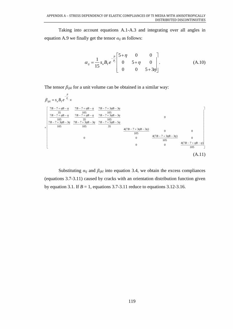
APPENDIX A – STRESS DEPENDENCY OF ELASTIC COMPLIANCES OF TI MEDIA WITH ANISOTROPICALLY DISTRIBUTED DISCONTINUITIES
119
Taking into account equations A.1-A.3 and integrating over all angles in
equation A.9 we finally get the tensor αij as follows:
3500
050
005
15
1cP
P
Tnij eBs . (A.10)
The tensor βijkl for a unit volume can be obtained in a similar way:
cP
P
Tnijkl eBs
105
)77(400
0105
)3377(400
00105
)3377(435
5577
105
3377
105
3377
0105
3377
35
77
105
77105
3377
105
77
35
77
BB
BB
BB
BBBBBB
BBBBBB
BBBBBB
(A.11)
Substituting αij and βijkl into equation 3.4, we obtain the excess compliances
(equations 3.7-3.11) caused by cracks with an orientation distribution function given
by equation 3.1. If B = 1, equations 3.7-3.11 reduce to equations 3.12-3.16.

APPENDIX B – ACKNOWLEDGEMENTS
120
APPENDIX B
SEG PUBLICATIONS
Letter from Ted Bakamjian
Director, Publications
Society of Exploration Geophysicists
From: Ted Bakamjian <[email protected]>
Sent: Friday, 1 May 2015 10:34 AM
To: Pavel Golodoniuc <[email protected]>
Cc: Permissions <[email protected]>
Subject: Re: Permission to use copyright material
Greetings Pavel,
Please find the permission you request in the attached form.
Sincerely,
Ted
--
Ted Bakamjian, IOM CAE
Director, Publications
Society of Exploration Geophysicists
P. O. Box 702740, Tulsa, OK 74170-2740 USA
Shipping: 8801 S. Yale Ave., Suite 500, Tulsa, OK 74137
Phone: (918) 497-5506; Fax: (918) 497-5557
Web: http://www.seg.org/
SEG Digital Library: http://library.seg.org
APPENDIX B – ACKNOWLEDGEMENTS
121
PERMISSION TO USE COPYRIGHT MATERIAL AS SPECIFIED BELOW
Pervukhina M., Gurevich B., Golodoniuc P., and Dewhurst D. N., 2010,
Parameterization of elastic stress sensitivity in shales: Geophysics, 76(3), p.
WA147–WA155, doi:10.1190/1.3554401,
http://dx.doi.org/10.1190/1.3554401.
Pervukhina M., Gurevich B., Golodoniuc P., and Dewhurst D. N., 2011,
Stress dependency of elastic properties of shales: the effect of uniaxial stress:
SEG Extended abstract, San Antonio, USA, doi:10.1190/1.3627669,
http://dx.doi.org/10.1190/1.3627669.
Pervukhina M., Golodoniuc P., Gurevich B., Clennell M. B., Dewhurst D. N.,
and Nordgård Bolås H. M., 2015, Prediction of sonic velocities in shale from
porosity and clay fraction obtained from logs – a North Sea well case study:
Geophysics, 80(1), p. D1-D10, doi:10.1190/GEO2014-0044.1,
http://dx.doi.org/10.1190/geo2014-0044.1.
I hereby give permission for Pavel Golodoniuc to include the
abovementioned material(s) in his higher degree thesis for the Curtin University of
Technology, and to communicate this material via the Australasian Digital Thesis
Program. This permission is granted on a non-exclusive basis and for an indefinite
period.
I confirm that I am the copyright owner of the specified material.
Permission to use this material is subject to the following conditions:
Please include DOI-based permalinks in citations for these articles. Please
also ensure that the links are live in online versions of your theses. Also, please
acknowledge SEG copyright and that the papers are reprinted with SEG permission.
Thank you for publishing in Geophysics. Best of luck with your thesis.
Signed:
Name: Ted Bakamjian
Position: SEG Director, Publications
Date: 1/05/2015

APPENDIX B – ACKNOWLEDGEMENTS
122
Copyright permissions statement from
http://www.seg.org/resources/publications/permissions
PERMISSIONS
SEG publishes journals, books, and digital works with the primary aim of
disseminating research in and theory and applications of applied geophysics.
Consistent with this objective, the Society provides mechanisms for those who seek
to reuse or republish material from SEG publications while protecting the viability of
the SEG publications program. Any further questions about permissions can be sent
via email to the SEG publications department at [email protected].
Fair use
Authors and publishers may present or republish up to two figures or tables
per SEG article or per SEG book without seeking written permission from SEG,
provided that full acknowledgment of the source is provided in the new work. If SEG
has cited a publication for which it is not the publisher, rights should be obtained
from that publisher. SEG considers this fair use. There are no fees associated with
this permission. Authors who need documentation that SEG is extending this
permission are encouraged to print this message and present it to their publishers.
Those who require further documentation should contact the SEG publications
director. Requests to use any portion of "Seismic Data Analysis: Processing,
Inversion, and Interpretation of Seismic Data" should be directed to the SEG
publications director.
Permission granting
Those seeking permission to republish more material than described above
should contact the SEG publications director. Such requests should include complete
citations of works for which permission to republish is sought. If permission for
specific figures or tables is sought, please provide figure and table numbers.
Requests should include a description of the work in which the SEG material would
be republished. Information about the audience and the intended distribution also
should be included. The requests should be prepared on institutional letterhead if the

APPENDIX B – ACKNOWLEDGEMENTS
123
requesting party is representing an institution. License fees are assessed only when
the request is for a large amount of material or when the proposed usage is
commercial in nature or would limit SEG's market. If a license fee is assessed, it
must be paid prior to use or the permission is void.
Purchase redistribution rights online
Those seeking to redistribute SEG publications or portions thereof in print, by
fax, or online may purchase permission to do so online. SEG publications are
registered with the Copyright Clearance Center, and licenses to redistribute SEG
articles and portions of books are obtained through this nonprofit agency. Special
pricing is available for university professors, including license to distribute SEG
material through electronic course packs. Licenses also are available for distribution
of journal articles and expanded abstracts via email or posting on Intranets and
Extranets for limited time periods.
Authors' right to redistribute
Authors of articles in Geophysics, Interpretation, The Leading Edge, and the
Technical Program Expanded Abstracts may post their own articles on their personal
Web sites or the Web sites of their institutions without obtaining further permission
from SEG. Authors of journal articles and Expanded Abstracts retain similar rights
for print redistribution. If an author or an author's institution redistributes an author's
article online or in print, the original publication venue encompassed in a complete
citation and including SEG's status as publisher must be identified. Authors of SEG
books, or portions of SEG books, must seek permission from the SEG publications
director to redistribute these works in any form. Such permission will not be
withheld if SEG's investment in the original publication of the works is not
threatened. Questions should be directed to the publications director.