rspa.royalsocietypublishing.org

ResearchCite this article: Haghpanah B,Papadopoulos J, Mousanezhad D,Nayeb-Hashemi H, Vaziri A. 2014 Buckling ofregular, chiral and hierarchical honeycombsunder a general macroscopic stress state. Proc.R. Soc. A 470: 20130856.http://dx.doi.org/10.1098/rspa.2013.0856

Received: 23 December 2013Accepted: 14 April 2014

Subject Areas:mechanical engineering,structural engineering

Keywords:instability, cellular structure, beam-column,in-plane loading

Author for correspondence:Ashkan Vazirie-mail: vaziri@coe.neu.edu

Electronic supplementary material is availableat http://dx.doi.org/10.1098/rspa.2013.0856 orvia http://rspa.royalsocietypublishing.org.

Buckling of regular, chiraland hierarchical honeycombsunder a general macroscopicstress stateBabak Haghpanah, Jim Papadopoulos,

Davood Mousanezhad, Hamid Nayeb-Hashemi

and Ashkan Vaziri

Department of Mechanical and Industrial Engineering,Northeastern University, Boston, MA, USA

An approach to obtain analytical closed-formexpressions for the macroscopic ‘buckling strength’of various two-dimensional cellular structures ispresented. The method is based on classical beam-column end-moment behaviour expressed in a matrixform. It is applied to sample honeycombs with square,triangular and hexagonal unit cells to determine theirbuckling strength under a general macroscopicin-plane stress state. The results were verified usingfinite-element Eigenvalue analysis.

1. IntroductionLow-density cellular materials have found widespreadapplication for energy absorption, structural protectionand as the core of lightweight sandwich panels.However, compressive loads can cause the cell wallsto buckle, which limits their strength. Collapse of thecellular material due to the buckling becomes morelikely as relative density is reduced [1]. Additionally,microscopic instability patterns could be deliberatelyused as a technique for induction or modification ofmicroscopic, periodicity-dependent structural or surfaceproperties such as chirality [2–4], wave propagationand phononic properties [5–11], optical characteristics[12–15], modulated nano patterns [16], hydrophobicity[17–20] or generating macroscopic responses [21,22] inperiodic solids. We thus see value in a general techniqueto predict the instability of regular cellular structuressubjected to a general macroscopic state of stress.

2014 The Authors. Published by the Royal Society under the terms of theCreative Commons Attribution License http://creativecommons.org/licenses/by/3.0/, which permits unrestricted use, provided the original author andsource are credited.

on July 3, 2018http://rspa.royalsocietypublishing.org/Downloaded from

2

rspa.royalsocietypublishing.orgProc.R.Soc.A470:20130856

...................................................

(iii)

(a)

(b)

(iv)

(v)(i)

(ii)

x

y

a

b

c

a'

b'

c'

q

Maqa

qb

Mb

P

N

N

P a

b

L

L L

L

L

Figure 1. (a) Types of lattice structures analysed by the beam-columnmatrix method: (i) square grid (§4a); (ii) triangular grid(isogrid—§4b); (iii) hexagonal honeycomb (§4c); (iv) hierarchical hexagonal honeycomb (electronic supplementary material,appendix C) and (v) tri-chiral honeycomb (electronic supplementary material, appendix D). The angle θ gives the orientationof straight walls in the tri-chiral lattice. (b) The angles of rotation and moments of the ends (positive when counter clockwise)in a beam-column.

Previous studies on the buckling of periodic cellular structures were largely numerical orexperimental. Ohno et al. [23] suggested a numerical method to study the buckling of cellularsolids subjected to macroscopically uniform compression using a homogenization frameworkof the updated Lagrangian type. Triantafyllidis & Schraad [24] studied the onset of failure inhoneycombs under general in-plane loading using finite-element (FE) discretization of Blochwave theory. Abeyaratne & Triantafyllidis [25] associated instability of periodic solids with theloss of ellipticity in the incremental response of homogenized deformation behaviour. A full-scale FE study of intact and damaged hexagonal honeycombs has been presented by Guo &Gibson [26]. Several experimental studies have concerned the buckling of different cellularstructures including hexagonal and circular honeycombs [27–33].

This study does not address localized buckling patterns in cellular materials (e.g. row wise)that can occur due to the presence of imperfections [24], boundary effects [34] or materialnonlinearity [32]. However, the collapse surfaces obtained here for periodic buckling patternsin perfect cellular materials provide an upper bound for the onset of failure in the correspondingactual materials that contain inevitable imperfections in their underlying microstructures [24].The analytical method presented here is inspired by research of Gibson et al. [35] on the stabilityof regular hexagonal honeycombs under in-plane macroscopic biaxial stress parallel to materialsymmetry directions (i.e. x and y in figure 1) using the beam-column solution of Manderla &Maney [36,37], as presented by Timoshenko & Gere [38]. In §2, we express the beam-columnresult in matrix form, to develop analytical closed-form expressions of the microscopic bucklingstrength for periodic beam structures under a general in-plane loading. In §3, the FE analysisused to verify the analytical results is explained. In §4, the proposed analytical approach is usedto predict buckling of regular square, triangular and hexagonal honeycombs as shown in figure 1.(The illustrated hierarchical and tri-chiral hexagonal honeycombs are treated in the electronicsupplementary material, appendices for the sake of brevity but the results are summarized here.)

on July 3, 2018http://rspa.royalsocietypublishing.org/Downloaded from

3

rspa.royalsocietypublishing.orgProc.R.Soc.A470:20130856

...................................................

The periodic square grid is also shown to buckle according to long-wave macroscopic patternsunder certain boundary conditions [39], a phenomenon observed in some three-dimensionalfoams [40]. Therefore, we also calculate its long-wave buckling strength under arbitrary loadingas the wavelength approaches infinity. Conclusions are drawn in §5.

2. MethodA unit cell, or a primitive cell in classical physics, is the smallest structural unit, by assemblingwhich the undeformed geometrical and loading patterns in a tessellated solid are recreated.When cellular solids are subjected to loading, buckling may occur in cell walls and edges, with adeformation pattern repeated on finite wavelengths. This kind of buckling, known as microscopicbuckling, is repeated over wavelengths which can be longer than the unit cell [41]. Such mode-size repeating patterns in the buckled structure are widely known as representative volume elements(RVEs) and might be different under various macroscopic loading conditions applied to thestructure [42]. In order to obtain the periodicity of a buckled tessellated structure, variousapproaches including Bloch wave analysis [24,43,44], block-diagonalization [45], Eigenvalueanalysis on RVEs of progressively increasing size [43,46], full-scale FE analysis [24,26,30,47] andexperimental investigations [28,29,32,33] have been used.

The methods proposed here for obtaining closed-form expressions of macroscopic bucklingstrength are based on ‘assumed’ buckling modes, providing the size of RVE and its overallbuckled geometry. Fortunately, the number of different buckling modes observed for a cellularstructure under different macroscopic loadings is usually small. For instance, just two microscopicbuckling patterns are found in the literature for square, triangular and hexagonal honeycombsunder various loading conditions.

(a) Beam-column end momentsThe beam-column formula is a classical approach linking the end rotations of an axially loadedbeam to its end moments. This approach has been used to obtain the buckling strength of cellularstructures under simplified loading conditions, including uniaxial and biaxial loadings [35,48].However, the complexity of an arbitrary stress state complicates the beam-column equations,especially for larger RVEs with higher nodal connectivity. In this section, we present thecharacteristic nonlinear beam-column equations in a matrix form, allowing a more systematiccalculation of the buckling strength. The symbolic calculation tool in MATLAB is then used toobtain closed-form expressions of buckling strength.

For a single beam connecting nodes a and b under axial compressive force P and subjected tothe two counter clockwise end couples Ma and Mb, the end rotations θa and θb (positive whencounter clockwise) relative to the line joining the displaced end nodes (figure 1b) can be obtainedthrough the beam-column relations as [38]

θa = +MalEI

Ψ (q) − MblEI

Φ(q)

and θb = −MalEI

Φ(q) + MblEI

Ψ (q).

⎫⎪⎪⎬⎪⎪⎭

(2.1)

Here, Φ(q) = (1/ sin q − 1/q)/q and Ψ (q) = (1/q − 1/ tan q)/q are nonlinear functions of the non-dimensional loading parameter q defined as q = l

√P/(EI), where P is the beam axial force (positive

when compressive), l is the beam length and EI is the beam flexural rigidity. The functions Φ andΨ can be approximated by even-order expansions, climbing monotonically from Φ = 1/6 andΨ = 1/3 when q = 0 to infinity when q = π .) Taking the rigid body rotation β of the beam (i.e.the line joining the beam ends) as an additional degree of freedom, the set of three boundaryconditions (i.e. two on beam end displacements or moments, and one on beam rotation β) andtwo beam-column relations given in equation (2.1) can be expressed in the following matrix form

on July 3, 2018http://rspa.royalsocietypublishing.org/Downloaded from

4

rspa.royalsocietypublishing.orgProc.R.Soc.A470:20130856

...................................................

to obtain the buckling of a single beam under axial loading:

[A]5×5

⎡⎢⎢⎢⎢⎢⎢⎢⎣

Mal/EI

Mbl/EI

θa

θb

βab

⎤⎥⎥⎥⎥⎥⎥⎥⎦

5×1

= [B]5×1. (2.2)

Here, matrix A is termed the system’s characteristic matrix, and the condition |A| = 0 gives thecritical value of q and hence the buckling load Pc. Vector B contains any loading terms appearingin the problem which do not explicitly include any beam end moments, beam end rotations oraxial loads. From the physical point of view, components of vector B are terms which only causea static deflection without buckling (e.g. a transverse load component applied to the tip of acantilevered axially loaded beam-column). Vector B does not affect the magnitude of the criticalloads obtained from Eigenvalue buckling analysis (electronic supplementary material, appendixA shows how this matrix representation can be used for solving standard single-column bucklingproblems.)

For the case of a cellular structure’s RVE consisting of several beams and connecting nodes, therelationships between nodal rotations and end moments for each beam, and also the boundaryconditions, can be assembled in the following general matrix form:

[A]n×n

⎡⎢⎢⎢⎢⎣

Ml/EIθ

β

...

⎤⎥⎥⎥⎥⎦

n×1

= [B]n×1. (2.3)

The condition |A| = 0 gives the relationship between the magnitudes of axial load for the beamsinside a RVE that cause it to become unstable. When [B] = 0 or small, this instability condition(i.e. |A| = 0) translates to the possibility of unlimited increase in values of nodal (or beam)rotations or beam end moments at finite, fixed values of beam axial loads. When [B] is non-zeroand sufficiently large, the bifurcation response is suppressed by a static, stable deformation ofthe structure. Therefore, while the condition |A| = 0 is mathematically sufficient to predict anEigenvalue buckling, both |A| = 0 and [B] = 0 have to be simultaneously satisfied for an idealbifurcation in the load–displacement response. Analysis of the existing experimental data [49]on rubber honeycombs with hexagonal cells marks the possibility of buckling at non-zero, butrelatively small, values of [B].

3. Finite-element simulationsFE Eigenvalue buckling analysis was performed to validate the closed-form estimates of bucklingstrength. Two-dimensional elastic beam element models of the RVE were constructed using theFE software ABAQUS. These small RVE models were subjected to external loads derived fromstatic analysis of the structure subjected to arbitrary states of macroscopic stress. (For the caseof the statically indeterminate triangular grid, conditions from the periodicity of the unit cell areadditionally required [50].) Rotation and displacement constraints following from the periodicityof the RVE for each buckling mode were also applied to the outer nodes. A mesh sensitivityanalysis was carried out to ensure that the numerical solutions are mesh-independent. As thereis little data on the in-plane buckling behaviour of hierarchical and tri-chiral honeycombs, large-scale FE models of these structures were developed initially, to determine their modes of bucklingand the RVE size (see §2 for criteria for determining the RVE).

on July 3, 2018http://rspa.royalsocietypublishing.org/Downloaded from

5

rspa.royalsocietypublishing.orgProc.R.Soc.A470:20130856

...................................................

a

ag

b

b

b

bg

gg

a

a

AA

O

B

B

AO

a-bb

g

O

B

a-gA

OPx Px

Px

Px

a

L/2

MOA

MOA

MAO MOB

MBO

Pxy

Pxy

Pxy

Pxy

Pxy

Py

Pxy

Py

Pxy

L/2 L/2

L/2

L/2

L/2

L / 2

L/2

L/2

L/2 L/2

B

O

Py

Py

Pxy

ab

L/2

MOB

a

bb

Pxy Pxy

Py

Pxy

M/2

a-b

Py

Pxy

b

M/2Px

Px

II (non-swaying)I (swaying)

III (long wave)

A

A

B

B

a

a

b

O

bg

RVERVE

x

y

RVE

(a) (b)

(c)

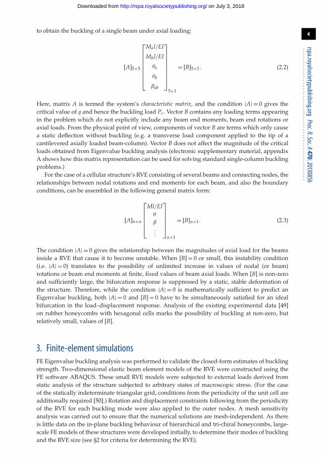
Figure2. (a–c) Themicroscopic bucklingmodes for the squaregrid. TheRVE in eachmode is denotedbybold lines. Notations forthe beamand nodal rotation in the RVE for eachmode are given in the top right. Free-body diagrams of the RVE beam-elementsare given in the bottom. (Online version in colour.)

4. Buckling of cellular structures under a general macroscopic stress stateAs examples of the method outlined in §2, the buckling stresses of some two-dimensionalcellular structures including hexagonal honeycombs and square and triangular grids (figure 1)are computed.

(a) Square honeycombsWah [51] first studied the stability of finite-size rectangular gridworks for both in-plane and out-of-plane loadings. Under uniaxial compressive loading parallel to cell walls, the strength of asquare grid according to the sway of the axially loaded cell walls (figure 2a) was estimated asSc/Es = (π2/12) ∗ (t/L)3, where cell walls of length L are treated as side-swaying columns withfixed slope at both ends [52]. This is an upper bound estimate of the actual buckling strengthof square grid structure since it ignores structural rotational compliance that actually permits

on July 3, 2018http://rspa.royalsocietypublishing.org/Downloaded from

6

rspa.royalsocietypublishing.orgProc.R.Soc.A470:20130856

...................................................

slope change. Fan et al. [48] calculated the uniaxial buckling strength of square honeycombs forthe two numerically observed microscopic buckling patterns, swaying and non-swaying modes,using the beam-column method (figure 2a,b). They expressed the uniaxial buckling strengthsof the structure as SIc/Es = ((0.76 ∗ π )2/12) ∗ (t/L)3 and SIIc/Es = ((1.292 ∗ π )2/12) ∗ (t/L)3, withthe mode I strength being less than the upper bound solution from [52]. Also, the long-wavebifurcation in square honeycombs under in-plane loading was previously studied through atwo-scale theory of the updated Lagrangian type by Ohno et al. [39]. They showed that unlikehexagonal honeycombs, the long-wave buckling patterns in periodic square honeycombs couldoccur at loads lower than the critical loads corresponding to some microscopic buckling patterns.According to their analysis, by increasing the wavelength to infinity the buckling strength undereither uniaxial or biaxial loadings parallel to material directions (i.e. x and y in figure 1) wouldapproach Sc/Es = (1/2) ∗ (t/L)3 (where the structures buckle due to the higher principal stressand ignore the lower). The buckling wavelength for long-wave buckling patterns is shown to bedependent on the size of the finite structure and also on the boundary conditions applied to afinite structure [39].

Here, for the first time we derive closed-form relations for the microscopic buckling patternsin the square grid, as well as the long-wave buckling patterns under general in-plane loadingconditions. For example, we show that under equi-biaxial (Sx = Sy) macroscopic loading thebuckling strength (Sx) of a square grid is Sx

c/Es = 0.453 ∗ (t/L)3; for pure shear (Sx = −Sy, Sx > 0) itis Sx

c/Es = 0.493 ∗ (t/L)3.

(i) Mode I (swaying)

Sway buckling shown in figure 2a is a shear deformation with only one set of beams changingtheir mean orientation, as expected for an overloaded building frame where the groundconnection keeps the horizontal beams level. By making cuts through cell wall midpoints, internalreaction forces per unit depth (positive when compressive) in the beams’ axial and transversedirections, denoted Px, Py and Pxy in figure 2a, are obtained for a square grid of beam length L [1]

⎡⎢⎢⎣

Px

Py

Pxy

⎤⎥⎥⎦ = −L

⎡⎢⎢⎣

1 0 0

0 1 0

0 0 1

⎤⎥⎥⎦

⎡⎢⎢⎣

σxx

σyy

τxy

⎤⎥⎥⎦ . (4.1)

Consequently, the non-dimensional x- and y-direction beam axial loading parameters qx and qy

are obtained as qx = L/2 ∗ √Px/(EI) = i

√3σ̄xx and qy = L/2 ∗ √

Py/(EI) = i√

3σ̄yy, where i = √−1and the stresses are normalized according to σ̄ = (σ/E)/(t/L)3.

For the swaying mode of buckling due primarily to compressive y stress, the RVE consistsof horizontal beam type OA and vertical beam type OB, as shown in figure 2a. These beams,respectively, experience end moments MOA and MOB at node O, and because of 180◦ rotationalsymmetry at the outer nodes A and B are moment-free there. The unknown rotation of node Ois defined as −α. Then the beam-column and equilibrium relations of the different beam typesOA and OB can be expressed in the matrix form given below. The first row expresses the beam-column relation for rotation −α of end O of OA, where there is a moment at O only, and overallbeam rotation β is zero. The second row, for the relative rotation β − α of end O of beam OB,again has a moment at O only, but this time rotation β is non-zero. The third row corresponds tothe moment equilibrium of node O, and the last row expresses the moment equilibrium of beamOB about point O

⎡⎢⎢⎢⎢⎣

−Ψ (qx)/2 0 1 0

0 −Ψ (qy)/2 1 −1

1 1 0 0

0 −1 0 −2q2y

⎤⎥⎥⎥⎥⎦

A

⎡⎢⎢⎢⎢⎣

MOAL/(EI)

MOBL/(EI)

α

β

⎤⎥⎥⎥⎥⎦ =

⎡⎢⎢⎢⎢⎣

0

0

0

−PxyL2/(2EI)

⎤⎥⎥⎥⎥⎦

B

. (4.2)

on July 3, 2018http://rspa.royalsocietypublishing.org/Downloaded from

7

rspa.royalsocietypublishing.orgProc.R.Soc.A470:20130856

...................................................

–2

–1

0

1

–2 –1 0 1 2

2

(a) (b)

–1

0

1

non-

buck

ling z

one

S yy /E

/(t/

L)3

S xy /E

/(t/

L)3

Sxx /E/(t/L)3

Sxx /E/(t/L)3

Syy /E/(t/L) 3

FE resultsprevious data

x

y –1

0

1

2

0–1

12

Figure 3. (a) Buckling of square honeycomb under x–y biaxial loading according to swaying, non-swaying and long-wavemodes of buckling. (b) The buckling collapse surface for the square grid in the σxx − σyy − τxy stress space, allowingprediction of buckling strength under a general in-plane state of stress. The left- and right-hand sides of the instability surfacecorrespond to the sway of horizontal and vertical beams. The condition [B]= 0 is marked by dashed lines on the instabilitysurface. (Online version in colour.)

For buckling to occur, i.e. for α and β to spontaneously take on non-zero values, the determinantof matrix A must vanish due to its dependence on the loads, i.e. qx and qy. The relation for thethreshold of in-plane instability in a square grid according to the swaying mode (mode I) ofbuckling with the x-direction beams held level is therefore

1

q2x

(1 − qx

tan(qx)

)− 1

q2y

(qy

tan(qy)

)= 0. (4.3a)

This relation is plotted in figure 3a, where it can be seen that x tension is very slightly protectiveagainst sway of y-direction beams due to y compression. A second relation is required for thesway of x-direction beams

1

q2y

(1 − qy

tan(qy)

)− 1

q2x

(qx

tan(qx)

)= 0. (4.3b)

Note that Pxy is irrelevant to the question of buckling, since it appears only on the right-handside of equation (4.2). However, it leads to unbounded α and β as matrix A approaches singularity.Substituting from qx = i

√3σ̄xx and qy = i

√3σ̄yy into equations (4.3) yield the following relations for

the first-mode buckling of a square grid

σ̄yy

(1 −

√3σ̄xx coth

(√3σ̄xx

))− σ̄xx

(√3σ̄yy coth

(√3σ̄yy

))= 0 (4.4a)

andσ̄xx

(1 −

√3σ̄yy coth

(√3σ̄yy

))− σ̄yy

(√3σ̄xx coth

(√3σ̄xx

))= 0. (4.4b)

(ii) Mode II (non-swaying)

Non-swaying buckling involves x and/or y compressive buckling with no macroscopic shearingdeformation. This requires cooperative buckling in adjacent cells to minimize energy. The samedefinitions of Px, Py, Pxy, qx and qy are used as above. Figure 2b shows the non-swaying mode(mode II) with the structural RVE indicated by red lines, as well as the free-body diagram of theRVE. Now the beam midpoints are not moment-free, so both MOA and MAO come into play. (Notethe altered sign convention for MOA.)

on July 3, 2018http://rspa.royalsocietypublishing.org/Downloaded from

8

rspa.royalsocietypublishing.orgProc.R.Soc.A470:20130856

...................................................

The set of beam-column relations can be expressed in the following matrix form. The firsttwo rows express moment equilibrium of beams OA and OB about point O. Rows three to sixrepresent the beam-column relations for relative rotation of both ends of beams OA and OB. Thelast row expresses the moment equilibrium of node O

⎡⎢⎢⎢⎢⎢⎢⎢⎢⎢⎢⎢⎢⎢⎢⎢⎢⎢⎢⎣

−1 1 0 0 0 −2q2x 0

0 0 −1 1 0 0 −2q2y

Φ(qx)2

Ψ (qx)2

0 0 0 −1 0

Ψ (qx)2

Φ(qx)2

0 0 −1 1 0

0 0Φ(qy)

2Ψ (qy)

20 0 −1

0 0Ψ (qy)

2Φ(qy)

2−1 0 1

1 0 1 0 0 0 0

⎤⎥⎥⎥⎥⎥⎥⎥⎥⎥⎥⎥⎥⎥⎥⎥⎥⎥⎥⎦

⎡⎢⎢⎢⎢⎢⎢⎢⎢⎢⎢⎢⎢⎢⎣

MOAL/(EI)

MAOL/(EI)

MOBL/(EI)

MBOL/(EI)

α

β

γ

⎤⎥⎥⎥⎥⎥⎥⎥⎥⎥⎥⎥⎥⎥⎦

⎡⎢⎢⎢⎢⎢⎢⎢⎢⎢⎢⎢⎢⎣

−PxyL2/(2EI)

+PxyL2/(2EI)

0

0

0

0

0

⎤⎥⎥⎥⎥⎥⎥⎥⎥⎥⎥⎥⎥⎦

. (4.5)

Setting the determinant of the characteristic matrix to zero results in qx cot(qx) + qy cot(qy) = 0.Since this relation is symmetric in x and y (figure 3a), no additional expression is needed. Laterwe will see that the magnitudes of stresses satisfying this relationship are always greater thanthe stresses required for the swaying mode of buckling, described by equations (4.4). Therefore,the non-swaying buckling mode is never the preferred mode of buckling under macroscopicstress state.

(iii) Mode III (long-wave)

The long-wave mode of buckling was previously studied by Ohno and co-workers through FEdiscretization of a two-scale theory of the updated Lagrangian type [39,53,54]. They estimatedthe uniaxial onset stress of long-wave buckling for the square grid as Sx

LWc/Es = 0.5 ∗ (t/L)3. Here,the long-wave buckling strength of a square grid under a general stress state is sought as thewavelength approaches infinity, using the beam-column method. Figure 2c shows a deformedstructure according to this buckling pattern, where the RVE is defined as a cross-shaped unitconnecting four adjacent beam centres. Note that under the long-wave mode shown in this figureall vertical lines deform similarly. Also, the horizontal lines deform periodically over x with thedeflections equal to zero at the midpoints of each length-L segment. As a result, each verticalbeam can be independently analysed as an axially loaded vertical beam supported at a spacingof L along the height of the beam by horizontal beams of length L which are welded to thevertical beam at their centres. The horizontal beams can be considered to be simply supportedat both ends due to zero curvature but free to translate horizontally. As the buckling wavelength(along y) approaches infinity, the distance between horizontal beams become smaller with respectto the wavelength, and thus, the angular stiffening effect of the horizontal beams can be estimatedby analogy to an axially loaded vertical beam on a foundation of distributed rotational springs.Electronic supplementary material, appendix B details the differential relations governing theinstability of an axially loaded beam on a distributed rotational spring foundation of intensity Kt

(with the unit of moment per radian per unit length and dimension [N]), where it is shown thatthe critical compressive buckling load equals Pcr = Kt.

The goal here is therefore to obtain an equivalent rotational stiffness for the horizontalsegments which are supporting vertical beams using the beam-column method. Once the effectiverotational stiffness, Kt, is obtained, the buckling load can be calculated using Pcr = Kt. Figure 2cshows a free-body diagram of the RVE, where the central node is rotated by angle β and thevertical beam segment of length L has an equivalent rotation of α, as resisted by the moment M inthe middle as shown in the figure. Since each half-beam has a moment-free end, the set of beam-column relations for the RVE is α − β = (ML/(4EI)) ∗ Ψ (qy) and β = (ML/(4EI)) ∗ Ψ (qx), whereqx = L/2 ∗ √

Px/EI and qy = L/2 ∗ √Py/EI. The equivalent rotational stiffness of the horizontal

on July 3, 2018http://rspa.royalsocietypublishing.org/Downloaded from

9

rspa.royalsocietypublishing.orgProc.R.Soc.A470:20130856

...................................................

segments due to the swaying angle α can therefore be calculated as

Kt = MLα

= 4EIL2

1Ψ (qx) + Ψ (qy)

. (4.6)

Substituting into the Pcr = Kt identity, the relations between parameters qx and qy needed for thelong-wave instability of square grid based on the two variations along x and y are

q2x(Ψ (qx) + Ψ (qy)) = 1

and q2y(Ψ (qx) + Ψ (qy)) = 1.

⎫⎬⎭ (4.7)

These are mathematically identical to the relations obtained in equations (4.3) for buckling of thesquare grid according to the x or y swaying mode of instability. This approaching of the long-wave buckling strength to the swaying mode strength can also be justified from the physicalpoint of view. By increasing the buckling wavelength in an unbounded structure (figure 2c), thedeformation field corresponding to an arbitrary volume of n × n cells (n < ∞) approaches theuniform deformation field observed in the swaying mode of buckling.

(iv) Results

Figure 3a shows the buckling strength curves corresponding to the x and y swaying modes, andthe non-swaying buckling mode, in a square honeycomb under biaxial loading parallel to materialprincipal directions (i.e. x and y). The horizontal and vertical axes correspond to normalizednormal stresses in x and y, respectively, according to σ̄ = (σ/E)/(t/L)3. The green curve denotesthe non-swaying mode of buckling. The red lines correspond to the swaying microscopic bucklingmode (equally, the long-wave buckling mode). The equi-biaxial buckling strength of a square gridis estimated as S̄x

c = S̄yc = 0.453. The results are verified by the FE Eigenvalue analysis preformed

at full as well as RVE scales.Since three loading variables, Px, Py and Pxy, define the general in-plane loading, the results

can be plotted in three dimensions for an arbitrary macroscopic state of stress. In figure 3b, thebuckling surface of the square honeycomb is presented, which is described by the inner envelopeof buckling stresses corresponding to the two rotational variations of the swaying or long-wavemodes of buckling identically given by equations (4.4). The left- and right-hand sides of theinstability surface in this figure correspond to the sway of horizontal and vertical beams in thesquare grid, respectively. The Eigenvalue instability in a square grid is independent of the valueof shear loading, Pxy, since the shear component does not explicitly appear in equations (4.4).However, sufficiently large values of shear stress can suppress the bifurcation response in abiaxially loaded square grid parallel to material principal directions (i.e. x and y), since the shearload component yields non-zero [B] matrices in equations (4.2) and (4.5). The macroscopic stressstates corresponding to [B] = 0 are also marked in this figure by dashed lines, sufficiently largedeviations from which would cause the structure to deform according to a static, stable shear.

(b) Triangular honeycombsA similar approach was used to explore the buckling of triangular honeycomb. Differences occurin the number of beams in the RVE, and the possibility of two kinds of buckling pattern. Wang &McDowell [52] approximated the buckling strengths of a series of common cellular structures bymeans of a simplistic approach involving the equivalent beam length for cell walls of differentperiodic structures. They estimated the uniaxial buckling strength of triangular grid along any

of the three cell wall directions to be Sc/Es =(

2π2/3√

3)

∗ (t/L)3. Similar to the case of a squarehoneycomb, this is an upper bound estimate of the actual buckling strength since it suppresses therotations of the end nodes of the cell walls during buckling. More recently, Fan et al. [48] obtaineda more precise estimation of uniaxial buckling strength of triangular honeycombs using the beam-column approach which allows for the rotation of the end nodes of cell wall during buckling. Theyexpressed the uniaxial buckling strength along the cell wall direction (x) and the perpendicular

on July 3, 2018http://rspa.royalsocietypublishing.org/Downloaded from

10

rspa.royalsocietypublishing.orgProc.R.Soc.A470:20130856

...................................................

mode IImode I

Fb

Fb

a

a

MB

MB

a

Fb

Fb

MOB

MBO

a

Fc

Fc

MOC

MCO

aaFaFa

MOA MAO

(a) (b)

aa

aa

aa

aa

O

A

B

B

A

C

C

a

aa

aa

aa

a

a

a

a

a

C

L L

L

L

L

Fa Fa

a

a

MAMA L

Fc

Fc

a

a

MC

MC

L L

LL

C

AA

B

B

O

a

b

c

x

y

RVE

RVE

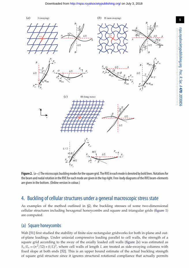
Figure4. (a,b)Modes I and II of buckling in triangular honeycomb, respectively. Inmode I, beam types OB andOChave oppositemoments at their ends, while beam types OA have the same moments at their ends. In mode II, beam types OB and OC havezero rotation at one end, while beam types OA have opposite moments at their ends. The RVE for eachmode is denoted by boldlines. Notations for the beam and nodal rotation in the RVE are given in the top right for each mode. Free-body diagrams of theRVE beam-elements are given in the bottom. (Online version in colour.)

to cell walls (y) as Sxc/Es = 2.543 ∗ (t/L)3 and Sy

c/Es = 2.876 ∗ (t/L)3, respectively. Here, for the firsttime we provide a simple formula for the in-plane buckling of triangular grid under a generalstress state.

(i) Mode I

For the sake of simplicity and also symmetrical results, the general state of in-plane macroscopicstress is uniquely expressed in terms of its normal lattice-direction components, σaa, σbb, σcc, inthe three in-plane material directions a = 0◦, b = 120◦ and c = 240◦ (measured from the x-axis)as shown in figure 1. Given these lattice-normal components of general stress tensor, themacroscopic xy stress tensor can be written as [55]

⎡⎣σxx τxy

τxy σyy

⎤⎦ =

⎡⎢⎢⎣

σaaσcc√

3− σbb√

3σcc√

3− σbb√

3

2σcc + 2σbb − σaa

3

⎤⎥⎥⎦. (4.8)

For example, uniaxial loadings σxx = σ and σyy = σ are represented by sets of (σa, σb, σc) stressesequal to (σ , σ/4, σ/4) and (0, 3σ/4, 3σ/4), respectively.

Based on FE computations, only the two buckling modes indicated as I and II in figure 4 appearin the triangular grid structure under various loading conditions. Mode I is characterized by theequal rotation of all nodes in a row (e.g. along a), while adjacent rows have opposite rotations.Mode II is distinguished by zero rotation of nodes and beams in every other row of the structureand the alternating rotation of adjacent nodes in the remaining rows. Note that mode shapes Iand II shown in figure 4 are unique with respect to direction a and symmetric relative to b and cdirections, so the entire collapse surface is defined by equivalent mode shapes along the a, b andc directions.

Wang & McDowell [50] provided the internal axial forces per unit depth (positive whencompressive) of beams in the equilateral triangular cell (isogrid) honeycomb of beam length L

⎡⎢⎢⎣

Fa

Fb

Fc

⎤⎥⎥⎦ = −L

⎡⎢⎢⎣

√3/2 −√

3/6 0

0√

3/3 −1

0√

3/3 1

⎤⎥⎥⎦

⎡⎢⎢⎣

σxx

σyy

τxy

⎤⎥⎥⎦, (4.9)

on July 3, 2018http://rspa.royalsocietypublishing.org/Downloaded from

11

rspa.royalsocietypublishing.orgProc.R.Soc.A470:20130856

...................................................

substituting from equation (4.8), we find the non-dimensional axial loading parametersqa = L

√Fa/(EI), qb = L

√Fb/(EI), qc = L

√Fc/(EI) for the beams oriented along the a, b and c

directions as follows:

qa = 2i√

5σ̄aa − σ̄bb − σ̄cc

31/4 , qb = 2i√

5σ̄bb − σ̄aa − σ̄cc

31/4 , qc = 2i√

5σ̄cc − σ̄aa − σ̄bb

31/4 . (4.10)

Here, stresses are normalized according to σ̄ = (σ/E)/(t/L)3. Since a triangular grid of inextensiblebeams can resolve all macroscopic loads with purely axial forces, load-induced beam transverseforces in this stretching dominated grid may be taken as zero.

The free-body diagram of a RVE for mode I buckling in a triangular grid is shown in figure 4a.In this mode, all nodes in a row rotate by the same angle. The a beams therefore have thesame moment and same angle at each end, so the beam-column relations for each end areidentical and only one is needed. Similarly, the b and c beams are symmetrically deformed withopposite moments and opposite relative angles, so the beam-column relations for each end arealso identical (apart from a sign change). Beam-column and equilibrium relations for all threetypes of beam can be expressed in the following matrix form, where the first three rows are thethree single beam-column relations for beams OA, OB and OC, and the last row expresses momentequilibrium for the central node O

⎡⎢⎢⎢⎢⎢⎣

1 −(Ψ (qa) − Φ(qa)) 0 0

1 0 −(Ψ (qb) + Φ(qb)) 0

1 0 0 −(Ψ (qc) + Φ(qc))

0 1 1 1

⎤⎥⎥⎥⎥⎥⎦

⎡⎢⎢⎢⎢⎢⎢⎢⎢⎢⎣

α

MALEI

MBLEI

MCLEI

⎤⎥⎥⎥⎥⎥⎥⎥⎥⎥⎦

=

⎡⎢⎢⎢⎢⎢⎣

0

0

0

0

⎤⎥⎥⎥⎥⎥⎦

. (4.11)

Equating the determinant of the characteristic matrix to zero, the relation governing mode Ibuckling can be obtained as

qb cot(qb

2

)+ qc cot

(qc

2

)+ q2

a2 − qa cot(qa/2)

= 0. (4.12a)

Similar expressions for the other two directions can be obtained by cyclically interchanging thesubscripts:

qc cot(qc

2

)+ qa cot

(qa

2

)+ q2

b2 − qb cot(qb/2)

= 0 (4.12b)

and

qa cot(qa

2

)+ qb cot

(qb

2

)+ q2

c2 − qc cot(qc/2)

= 0. (4.12c)

The buckling modes described by equations (4.12a–c) correspond to zero curvature at themidpoints of beams along the a, b and c directions, respectively.

(ii) Mode II

Figure 4b shows the RVE free-body diagram for mode II buckling. In this mode, alternate alines remain straight during the buckling. The set of beam-column and equilibrium equationcan be written in the following matrix form, where the first five rows represent the beam-columnrelations for beams OA, OB and OC, and the last row satisfies the equilibrium of moments around

on July 3, 2018http://rspa.royalsocietypublishing.org/Downloaded from

12

rspa.royalsocietypublishing.orgProc.R.Soc.A470:20130856

...................................................

node O

⎡⎢⎢⎢⎢⎢⎢⎢⎢⎢⎢⎣

1 −Ψ (qa) − Φ(qa) 0 0 0 0

1 0 −Ψ (qb) −Φ(qb) 0 0

0 0 Φ(qb) Ψ (qb) 0 0

1 0 0 0 −Ψ (qc) −Φ(qc)

0 0 0 0 Φ(qc) Ψ (qc)

0 1 1 0 1 0

⎤⎥⎥⎥⎥⎥⎥⎥⎥⎥⎥⎦

⎡⎢⎢⎢⎢⎢⎢⎢⎢⎢⎢⎢⎢⎢⎢⎢⎢⎢⎢⎣

α

MOALEI

MOBLEI

MBOLEI

MOCLEI

MCOLEI

⎤⎥⎥⎥⎥⎥⎥⎥⎥⎥⎥⎥⎥⎥⎥⎥⎥⎥⎥⎦

=

⎡⎢⎢⎢⎢⎢⎢⎢⎢⎢⎢⎣

0

0

0

0

0

0

⎤⎥⎥⎥⎥⎥⎥⎥⎥⎥⎥⎦

. (4.13)

Equating the determinant of the characteristic matrix to zero, the relation between components ofstress for mode II of buckling is

qa cot(qa

2

)+ qb cot

(qb

2

) (1 − qb cot qb

2 − qb cot(qb/2)

)+ qc cot

(qc

2

) (1 − qc cot qc

2 − qc cot(qc/2)

)= 0, (4.14a)

and cyclically for b and c directions

qb cot(qb

2

)+ qc cot

(qc

2

) (1 − qc cot qc

2 − qc cot(qc/2)

)+ qa cot

(qa

2

) (1 − qa cot qa

2 − qa cot(qa/2)

)= 0 (4.14b)

and

qc cot(qc

2

)+ qa cot

(qa

2

) (1 − qa cot qa

2 − qa cot(qa/2)

)+ qb cot

(qb

2

) (1 − qb cot qb

2 − qb cot(qb/2)

)= 0. (4.14c)

Geometrically, the three rotational variations of mode II buckling described by equations(4.14a–c) involve alternate straight beams along a (figure 4b), b and c directions in the buckledstate, respectively. For the variation of mode II buckling shown in figure 4b, for example,the straightness of alternate horizontal type a beams is a special condition implying reflectionsymmetry about x- and y-axes, which requires, in effect, that the internal moment in those beamsbe small (i.e. MBO ∼= MCO). This condition is only satisfied when the characteristic matrix issymmetric with respect to b and c directions (i.e. qb = qc), corresponding to a biaxial state ofloading in the principal material directions x and y. The necessity of a biaxial stress state forformation of mode II buckling in a triangular grid is also observed full-scale FE analysis, wherethe second mode of buckling described by equation (4.14a) is rapidly suppressed by adding the τxy

shear stress component. Similarly, the two other variations of mode II with straight beams along band c directions described by equations (4.14b,c) can only occur under microscopic biaxial loadingalong the b (and b⊥) and c (and c⊥) directions, respectively (the symbol ⊥ denotes perpendicular).

Under a general state of loading where no two loading parameters (i.e. qa, qb, qc) are equal,the macroscopic stresses required for the mode II of buckling given in equations (4.14) are equalor greater than those for the mode I of buckling given in equations (4.12). Under a biaxialstate of loading along material principal directions x and y (i.e. qb = qc), equation (4.14a) can bealgebraically simplified to equations (4.12b,c). It can be shown numerically that under the x–ybiaxial macroscopic loading with first principal stress along y (i.e. σ̄xx < σ̄yy), the first rotationalvariation of mode II buckling expressed by equation (4.14a), and the second and third rotationsof mode I buckling expressed by equations (4.12b,c) equally yield the minimum required stress,and therefore are preferred buckling modes. For the case of x–y biaxial loading with the firstprincipal stress along x (i.e. σ̄xx > σ̄yy), the first rotational variation of mode I buckling describedby equation (4.12a) requires the minimum stress and is consequently preferred.

on July 3, 2018http://rspa.royalsocietypublishing.org/Downloaded from

13

rspa.royalsocietypublishing.orgProc.R.Soc.A470:20130856

...................................................

–6 –4 –2 0 2 4 6–6

–4

–2

0

2

4

6

–2

0

2

20

–2

–2

0

2

(a) (b)

non-

buck

ling z

one

FE resultsprevious data

a

b

c

(–2.395, –2.395, –2.395)

x

y

S yy/E

/(t/L

)3

S cc/E

/(t/L

)3

Sbb /E/(t/L) 3

Saa/E /(t/L)3

Sxx/E /(t/L)3

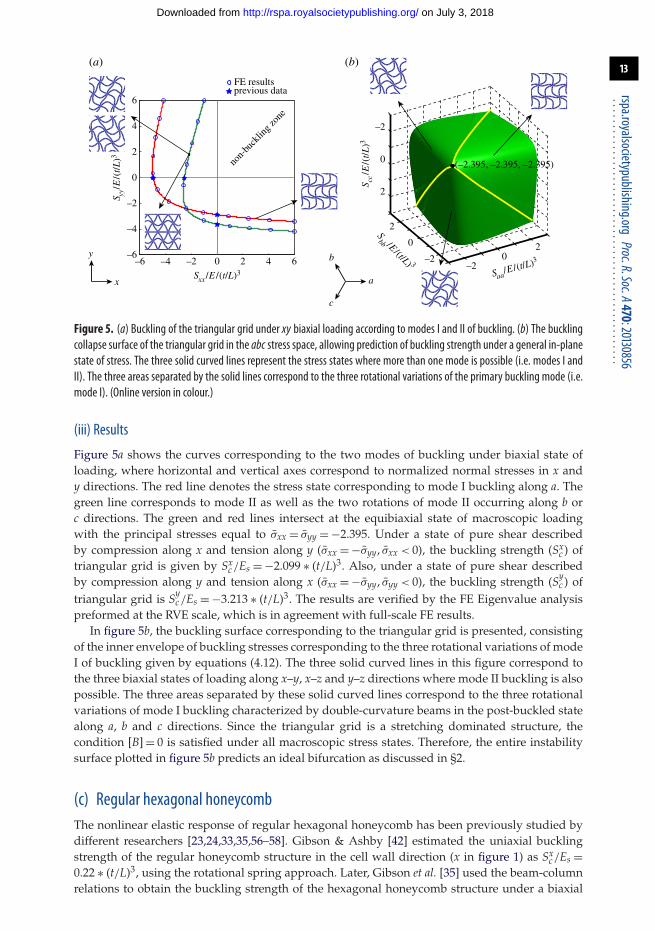
Figure 5. (a) Buckling of the triangular grid under xy biaxial loading according to modes I and II of buckling. (b) The bucklingcollapse surface of the triangular grid in the abc stress space, allowing prediction of buckling strength under a general in-planestate of stress. The three solid curved lines represent the stress states where more than one mode is possible (i.e. modes I andII). The three areas separated by the solid lines correspond to the three rotational variations of the primary buckling mode (i.e.mode I). (Online version in colour.)

(iii) Results

Figure 5a shows the curves corresponding to the two modes of buckling under biaxial state ofloading, where horizontal and vertical axes correspond to normalized normal stresses in x andy directions. The red line denotes the stress state corresponding to mode I buckling along a. Thegreen line corresponds to mode II as well as the two rotations of mode II occurring along b orc directions. The green and red lines intersect at the equibiaxial state of macroscopic loadingwith the principal stresses equal to σ̄xx = σ̄yy = −2.395. Under a state of pure shear describedby compression along x and tension along y (σ̄xx = −σ̄yy, σ̄xx < 0), the buckling strength (Sx

c ) oftriangular grid is given by Sx

c/Es = −2.099 ∗ (t/L)3. Also, under a state of pure shear describedby compression along y and tension along x (σ̄xx = −σ̄yy, σ̄yy < 0), the buckling strength (Sy

c ) oftriangular grid is Sy

c/Es = −3.213 ∗ (t/L)3. The results are verified by the FE Eigenvalue analysispreformed at the RVE scale, which is in agreement with full-scale FE results.

In figure 5b, the buckling surface corresponding to the triangular grid is presented, consistingof the inner envelope of buckling stresses corresponding to the three rotational variations of modeI of buckling given by equations (4.12). The three solid curved lines in this figure correspond tothe three biaxial states of loading along x–y, x–z and y–z directions where mode II buckling is alsopossible. The three areas separated by these solid curved lines correspond to the three rotationalvariations of mode I buckling characterized by double-curvature beams in the post-buckled statealong a, b and c directions. Since the triangular grid is a stretching dominated structure, thecondition [B] = 0 is satisfied under all macroscopic stress states. Therefore, the entire instabilitysurface plotted in figure 5b predicts an ideal bifurcation as discussed in §2.

(c) Regular hexagonal honeycombThe nonlinear elastic response of regular hexagonal honeycomb has been previously studied bydifferent researchers [23,24,33,35,56–58]. Gibson & Ashby [42] estimated the uniaxial bucklingstrength of the regular honeycomb structure in the cell wall direction (x in figure 1) as Sx

c/Es =0.22 ∗ (t/L)3, using the rotational spring approach. Later, Gibson et al. [35] used the beam-columnrelations to obtain the buckling strength of the hexagonal honeycomb structure under a biaxial

on July 3, 2018http://rspa.royalsocietypublishing.org/Downloaded from

14

rspa.royalsocietypublishing.orgProc.R.Soc.A470:20130856

...................................................

(a) mode I (uniaxial) (b)

b–a

b-aMa

Ma

O

O

L

AFa

Ga

Fa

Ga

qc

a–qb

qb

a–qc

a

aaa

O

B

L

L

C

A

mode II (biaxial)

RVE

(c)

Fa

a

Ma

Gaa

MaLFa

Ga

Fb

Fb

Gb

Gb

ab

B

gbL

b

b

a

a

a b

C

O

A

L

L

L

B

ga

gb

gc

L

Fa

Fa

Ga

Ga

Mao

Moa

b

aA

Oga

mode III (flower-like or chiral)

a

a

aa

a

b

b–aCA

B

O L

L

L

B

Fb

Fb

Gb

Gb

a

a

Mb

Mb

O

C

L

a

a

Mc

Mc

Fc

Gc

Fc

Gc

L

qc

a–qc

Fc

Fc

Gc

Gc

Moc

McoL

qb

a–qb

Fb

Fb

Gb

Gb

Mob

Mbo

ab

a

b

c

x

y

L

Fc

Fc

Gc

Gc

b

aC

Ogc

Moc

Mco

O

Mob

Mbo

LFbGb

b

FbGb

Mbo

Mbo

Fa

Ga

Mao

Fa

Ga

Mao

Fc

Gc

Fc

Gc

Mco

Mco

RVE

RVE

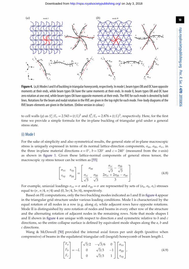
Figure 6. (a–c) Modes I, II and III of buckling observed in regular honeycomb, respectively. Modes I and II are characterizedby a zigzag collapse of cells due to compression along the x direction and an alternating cell collapse due to compressionperpendicular to the x direction, respectively. Mode III is a chiral cell configuration where groups of six highly deformed cellssurround almost intact central cells. The RVE for eachmode is denoted by bold lines. Notations for the beam and nodal rotationin the RVE for each mode are given in the top right. Free-body diagrams of the RVE beam-elements are given in the bottom.(Online version in colour.)

state of loading parallel to x and y directions. They recognized two modes of buckling, commonlyreferred to as uniaxial and biaxial, for elastic bifurcation of a hexagonal honeycomb structure(figure 6a,b). The large deformation of cell edges before elastic buckling was taken in account byZhang & Ashby [56] to analyse the biaxial in-plane buckling of hexagonal honeycombs. Ohno et al.numerically analysed the in-plane biaxial buckling of the regular hexagonal honeycomb usinga homogenization framework of updated Lagrangian type [23]. Triantafyllidis & Schraad [24]studied the onset of bifurcation in hexagonal honeycombs under general in-plane loading usingFE discretization of the Bloch wave theory. A third, more complex, flower-like mode, shownin figure 6c, is suggested for the buckling of regular hexagonal honeycomb structure [23].This mode of buckling has been previously observed in experimental and numerical trials forhexagonal honeycombs with circular cells under equi-biaxial loading condition [28,47]. In thismode of buckling, groups of six highly deformed cells surround almost intact central cells,and the central cells rotate uniformly in either the clockwise or the counter-clockwise direction.

on July 3, 2018http://rspa.royalsocietypublishing.org/Downloaded from

15

rspa.royalsocietypublishing.orgProc.R.Soc.A470:20130856

...................................................

Okumera et al. [58] later showed that the flower-like mode does not occur as the first bifurcationunder macroscopic biaxial compression control. Here, for the first time we obtain expressions ofbuckling strength for the uniaxial, biaxial and flower-like modes of buckling of the hexagonalhoneycomb structure under a general stress state.

(i) Mode I (uniaxial)

Because of the minimum threefold symmetry of regular honeycomb structure, the general stateof in-plane macroscopic stress is expressed in terms of its normal components, σaa, σbb, σcc, in thethree in-plane material directions a = 0◦, b = 120◦ and c = 240◦ from the x-axis as shown in figure 1.The macroscopic xy stress tensor can be expressed in terms of the normal components of stressin a, b and c directions according to equation (4.8). Also the axial forces per unit depth (positivewhen compressive) in the cell walls oriented along a, b, c directions can be expressed as [1]⎡

⎢⎢⎣Fa

Fb

Fc

⎤⎥⎥⎦ = −L

⎡⎢⎢⎣

√3 0 0

0√

3 0

0 0√

3

⎤⎥⎥⎦

⎡⎢⎢⎣

σaa

σbb

σcc

⎤⎥⎥⎦, (4.15)

where L is the size of the hexagon side. The non-dimensional parameters qa, qb and qc, are

therefore found as qa = L√

Fa/(EI) = 2i√

3√

3σ̄aa and cyclically for qb and qc. Also the transverseforces in the cell walls of the hexagonal honeycomb can be obtained according to [55]⎡

⎢⎢⎣Ga

Gb

Gc

⎤⎥⎥⎦ = 1√

3

⎡⎢⎢⎣

0 1 −1

−1 0 1

1 −1 0

⎤⎥⎥⎦

⎡⎢⎢⎣

Fa

Fb

Fc

⎤⎥⎥⎦. (4.16)

For mode I (uniaxial) buckling, the structural RVE shown in figure 6a consists of the threebeams OA, OB and OC oriented along a, b and c directions, respectively. The pre- and post-buckling configurations of the RVE are shown by red dashed lines and solid black lines,respectively. Taking into account the symmetry requirements in the buckled configuration of thestructure, beam OA is under equal end moments, denoted by Ma, and beams OB and OC eachare under opposite (with equal magnitude) end moments denoted by Mb and Mc, respectively, asshown in figure 6a. The set of beam-column and equilibrium relations of the three different bartypes OA, OB and OC can be expressed in the following matrix form, where the first three matrixrows represent the beam-column relations for beams OA, OB and OC, the fourth line correspondsto equilibrium of node O, and the last relation expresses moment equilibrium in beam OA aroundnode O.

⎡⎢⎢⎢⎢⎢⎢⎢⎣

−Ψ (qa) + Φ(qa) 0 0 −1 1

0 −Ψ (qb) − Φ(qb) 0 1 0

0 0 −Ψ (qc) − Φ(qc) 1 0

1 −1 −1 0 0

2 0 0 0 −q2a

⎤⎥⎥⎥⎥⎥⎥⎥⎦

⎡⎢⎢⎢⎢⎢⎢⎢⎢⎢⎢⎢⎢⎣

MaLEI

MbLEI

McLEIα

β

⎤⎥⎥⎥⎥⎥⎥⎥⎥⎥⎥⎥⎥⎦

=

⎡⎢⎢⎢⎢⎢⎢⎢⎢⎢⎣

0

0

0

0

−GaL2

EI

⎤⎥⎥⎥⎥⎥⎥⎥⎥⎥⎦

.

(4.17)Using the symbolic toolbox in MATLAB to set |A| = 0, the relation between qa, qb and qc expressingthe mode I instability of a regular honeycomb structure under a general loading is

qa tan(qa

2

)− qb cot

(qb

2

)− qc cot

(qc

2

)= 0. (4.18)

Therefore, the expression of mode I instability in the abc stress space would be

√σ̄aa tanh

(√3√

3σ̄aa

)+

√σ̄bb coth

(√3√

3σ̄bb

)+

√σ̄cc coth

(√3√

3σ̄cc

)= 0, (4.19a)

on July 3, 2018http://rspa.royalsocietypublishing.org/Downloaded from

16

rspa.royalsocietypublishing.orgProc.R.Soc.A470:20130856

...................................................

where the bar above the stresses means they are normalized according to σ̄ = (σ/E)/(t/L)3.Note that the uniaxial mode of buckling shown in figure 6a does not possess the threefoldsymmetry observed in the honeycomb lattice (i.e. the rotational symmetry with respect to thethree directions a, b and c), and therefore the following additional relations are needed to describethe buckling strength of a regular honeycomb according to uniaxial modes of buckling along b andc directions

√σ̄bb tanh

(√3√

3σ̄bb

)+

√σ̄cc coth

(√3√

3σ̄cc

)+

√σ̄aa coth

(√3√

3σ̄aa

)= 0 (4.19b)

and

√σ̄cc tanh

(√3√

3σ̄cc

)+

√σ̄aa coth

(√3√

3σ̄aa

)+

√σ̄bb coth

(√3√

3σ̄bb

)= 0. (4.19c)

From the geometrical point of view, the buckling modes described by equations (4.19) correspondto zero curvature at midpoints of beams along the a, b and c directions, respectively. Substitutingqb = qc in equations (4.19), the result given in [35] for the instability of a regular hexagonalhoneycomb under the simplified case of x–y biaxial loading condition is obtained.

(ii) Mode II (biaxial)

The biaxial mode of buckling and the associated RVE are shown in figure 6b. According tosymmetry requirements the beam OA is under opposite (with equal magnitude) moments,denoted by Ma, at the ends. Beams OB and OC are subjected to end moments Mob, Mbo, Moc, Mco,as shown in the figure. The set of beam-column and equilibrium relations of the three different bartypes OA, OB and OC can be expressed in the following matrix form, where the first five matrixrows represent the beam-column relations for beams OA, OB and OC, the sixth line correspondsto moment equilibrium of node O, and the last two relations satisfy the moment equilibrium inbeams OB and OC about node O.

⎡⎢⎢⎢⎢⎢⎢⎢⎢⎢⎢⎢⎢⎢⎢⎢⎣

−Φ(qa) − Ψ (qa) 0 0 0 0 1 0 0

0 −Ψ (qb) −Φ(qb) 0 0 0 1 0

0 −Φ(qb) −Ψ (qb) 0 0 1 −1 0

0 0 0 −Ψ (qc) −Φ(qc) 0 0 1

0 0 0 −Φ(qc) −Ψ (qc) 1 0 −1

1 1 0 1 0 0 0 0

0 1 −1 0 0 q2b −q2

b 0

0 0 0 1 −1 q2c 0 −q2

c

⎤⎥⎥⎥⎥⎥⎥⎥⎥⎥⎥⎥⎥⎥⎥⎥⎦

⎡⎢⎢⎢⎢⎢⎢⎢⎢⎢⎢⎢⎢⎢⎢⎢⎣

MaL/(EI)

MobL/(EI)

MboL/(EI)

MocL/(EI)

McoL/(EI)

α

θb

θc

⎤⎥⎥⎥⎥⎥⎥⎥⎥⎥⎥⎥⎥⎥⎥⎥⎦

=

⎡⎢⎢⎢⎢⎢⎢⎢⎢⎢⎢⎢⎢⎣

000000

GbL2/(EI)

GcL2/(EI)

⎤⎥⎥⎥⎥⎥⎥⎥⎥⎥⎥⎥⎥⎦

. (4.20)

Using the symbolic toolbox in MATLAB to set |A| = 0, the relation between qa, qb and qc expressingthe instability of a regular honeycomb structure in mode II under a general loading is

qa cot(qa

2

)+ qb cot(qb) + qc cot(qc) = 0, (4.21)

on July 3, 2018http://rspa.royalsocietypublishing.org/Downloaded from

17

rspa.royalsocietypublishing.orgProc.R.Soc.A470:20130856

...................................................

or considering all three rotations corresponding to this mode in the abc stress space√

σ̄aa coth(√

3√

3σ̄aa

)+

√σ̄bb coth

(2√

3√

3σ̄bb

)+

√σ̄cc coth

(2√

3√

3σ̄cc

)= 0, (4.22a)

√σ̄bb coth

(√3√

3σ̄bb

)+

√σ̄cc coth

(2√

3√

3σ̄cc

)+

√σ̄aa coth

(2√

3√

3σ̄aa

)= 0, (4.22b)

and√

σ̄cc coth(√

3√

3σ̄cc

)+

√σ̄aa coth

(2√

3√

3σ̄aa

)+

√σ̄bb coth

(2√

3√

3σ̄bb

)= 0, (4.22c)

Geometrically, the buckling modes described by equations (4.22a–c) include straight beams in thepost-buckled configuration along a, b and c directions, respectively.

The zero curvature in a series of horizontal beams in the post-buckled state shown in figure 6brequires the internal moment throughout those beams to be zero. Noting that the two pairsof opposite moments Mbo and Mco act on the ends of these beams, the last condition requiresMbo = Mco. This is only satisfied when the characteristic matrix is symmetrical with respect to band c directions, which translates to a biaxial state of loading in the principal material directions xand y. This is supported by full-scale FE analysis, where the mode II buckling is observed under x–y biaxial loading, and is rapidly suppressed by increasing the magnitude of macroscopic xy shearstress component. Given a biaxial state of macroscopic stress, equations (4.22) can be simplifiedto the result obtained in [35] for the instability of regular honeycomb under the simple case of x–ybiaxial loading condition.

(iii) Mode III (flower-like or chiral)

For the flower-like mode of buckling shown in figure 6c, the set of beam-column and equilibriumrelations of three different bar types OA, OB and OC can be expressed in the following matrixform, where the first and the second rows satisfy the moment equilibrium of node O and theintact central hexagon, respectively; rows three to five satisfy the moment equilibrium of beamsOA, OB and OC about O; and rows six to eleven represent the beam-column relations forbeams OA, OB and OC.

⎡⎢⎢⎢⎢⎢⎢⎢⎢⎢⎢⎢⎢⎢⎢⎢⎢⎢⎢⎢⎢⎢⎢⎣

1 1 1 0 0 0 0 0 0 0 0

0 0 0 1 1 1 0 −(q2a + q2

b + q2c ) 0 0 0

1 0 0 −1 0 0 0 0 q2a 0 0

0 1 0 0 −1 0 0 0 0 q2b 0

0 0 1 0 0 −1 0 0 0 0 q2c

Ψ (qa) 0 0 Φ(qa) 0 0 −1 0 1 0 0

0 Ψ (qb) 0 0 Φ(qb) 0 −1 0 0 1 0

0 0 Ψ (qc) 0 0 Φ(qc) −1 0 0 0 1

Φ(qa) 0 0 Ψ (qa) 0 0 0 −1 −1 0 0

0 Φ(qb) 0 0 Ψ (qb) 0 0 −1 0 −1 0

0 0 Φ(qc) 0 0 Ψ (qc) 0 −1 0 0 −1

⎤⎥⎥⎥⎥⎥⎥⎥⎥⎥⎥⎥⎥⎥⎥⎥⎥⎥⎥⎥⎥⎥⎥⎦

×

⎡⎢⎢⎢⎢⎢⎢⎢⎢⎢⎢⎢⎢⎢⎢⎢⎢⎢⎢⎢⎢⎢⎣

MoaL/(EI)

MobL/(EI)

MocL/(EI)

MaoL/(EI)

MboL/(EI)

McoL/(EI)

α

β

γa

γb

γc

⎤⎥⎥⎥⎥⎥⎥⎥⎥⎥⎥⎥⎥⎥⎥⎥⎥⎥⎥⎥⎥⎥⎦

=

⎡⎢⎢⎢⎢⎢⎢⎢⎢⎢⎢⎢⎢⎢⎢⎢⎢⎢⎢⎢⎢⎢⎣

0

(Ga + Gb + Gc)L2/(EI)

GaL2/(EI)

GbL2/(EI)

GcL2/(EI)

0

0

0

0

0

0

⎤⎥⎥⎥⎥⎥⎥⎥⎥⎥⎥⎥⎥⎥⎥⎥⎥⎥⎥⎥⎥⎥⎦

. (4.23)

on July 3, 2018http://rspa.royalsocietypublishing.org/Downloaded from

18

rspa.royalsocietypublishing.orgProc.R.Soc.A470:20130856

...................................................

2.0

1.5

1.0

0.5

0

–0.5

–1.0

–1.5

–2.02.01.51.00.50–0.5–1.0–1.5–2.0

0

–1.0–1.0–0.5

0.50

1.0

1.00.5

–0.5

–1.0

0

1.0

0.5

–0.5

(a) (b)

FE results

non-

buck

ling z

one

(–0.175, –0.175, –0.175)

a

b

cx

y

experiments [49]

S yy/E

/(t/L

)3

S cc/E

/(t/L

)3

Sxx /E /(t/L)3

Sbb /E /(t/L) 3

Saa/E /(t/L)3

Figure 7. (a) Biaxial buckling collapse of regular hexagonal honeycomb under biaxial loading along x (the so-called armchairor ribbon direction) and y (the so-called zigzag or transverse direction) according to uniaxial, biaxial and flower-like modes ofbuckling. The inset shows comparison with the experimental data from [49]. (b) The buckling collapse surface of the regularhoneycomb structure in the abc stress space, allowing prediction of buckling strength under a general in-plane state of stress.The three solid lines represent the stress states where more than one mode is possible (i.e. modes I and II). The three distinctareas on the buckling surface separated by the solid lines correspond to the three rotational variations of the primary bucklingmode (i.e. mode I). The condition [B]= 0 is marked by dashed lines on the instability surface. (Online version in colour.)

Equating the determinant of the characteristic matrix to zero yields the following relation betweenqa, qb and qc for flower-like instability of a regular hexagonal honeycomb

2

q2a + q2

b + q2c

+ 1qa tan(qa/2) + qb tan(qb/2) + qc tan(qc/2)

= 1qa cot(qa/2) + qbcot(qb/2) + qc cot(qc/2)

, (4.24)

where qa = 2i√

3√

3σ̄aa and cyclically for qb and qc.

(iv) Results

For all loading directions, each defined by a ratio between components of macroscopic stress,the stresses required for biaxial mode of buckling described by equations (4.22) are equal orgreater than those needed for the uniaxial mode of buckling given by equations (4.19). Underin-plane x–y biaxial loading (i.e. τ̄xy = 0 or equivalently σ̄bb = σ̄cc), equations (4.19b,c) can besimplified to equation (4.22a) using the trigonometric identity coth(2x) = ( coth(x) + tanh(x))/2.For a regular honeycomb structure under biaxial macroscopic loading with the first principalstress along x (i.e. σ̄xx > σ̄yy), the microscopic instability could arise through either the uniaxialmode with alternative swaying of beams along the a direction, or the biaxial mode involvingstraight beams along the a direction. In full-scale numerical trials, the buckling mode under thisloading condition is determined by the boundary conditions applied to the finite-size FE model.For the case of biaxial loading with the first principal stress along y (i.e. σ̄xx < σ̄yy), the uniaxialmode of buckling is the preferred mode.

Figure 7a shows the curves corresponding to uniaxial, biaxial and flower-like modes ofbuckling in a regular honeycomb under biaxial state of loading, where horizontal and verticalaxes correspond to normalized normal stresses in x and y directions, respectively, according toσ̄ = (σ/E)/(t/L)3. The green and red lines denote the uniaxial mode of buckling along a (or x)and the flower-like modes, respectively. The blue line corresponds to the biaxial mode as wellas the two variations of the uniaxial mode occurring along b or c directions. The green and

on July 3, 2018http://rspa.royalsocietypublishing.org/Downloaded from

19

rspa.royalsocietypublishing.orgProc.R.Soc.A470:20130856

...................................................

blue lines intersect at the equi-biaxial state of macroscopic loading with the principal stressesequal to σ̄xx = σ̄yy = −0.175. The flower-like mode is not a dominant mode under any loadingcondition. However, the macroscopic stresses needed for this mode become relatively close tothose of uniaxial and biaxial modes under equi-biaxial loading with the macroscopic stressesσ̄xx = σ̄yy = −0.198. The results are verified by the FE Eigenvalue analyses preformed at the RVEscale, which are in good agreement with full-scale FE results. The inset of the figure shows acomparison of the analytical results with experimental data from [49]. In figure 7b, the bucklingsurface for a regular hexagonal honeycomb structure under arbitrary stress state is presented. Thesurface is mathematically described by the inner envelope of buckling stresses corresponding tothe three rotational variations of the unixial mode (mode I) of buckling given by equations (4.19).The three edges marked by solid lines correspond to the three biaxial states of loading alongx–y, b (and b⊥) and c (and c⊥) directions, where the biaxial mode (mode II) of buckling is alsopossible. The three areas of the instability surface separated by these lines correspond to the threerotational variations of mode I buckling. On each edge, macroscopic stress states correspondingto the condition [B] = 0 in equation (4.17) are marked by dashed lines. Deviation from these lineswould cause the structure to fold up in a stable way. Note that for a mode II buckling the condition[B] = 0 in equation (4.20) is only satisfied under an equi-biaxial stress state.

5. ConclusionTable 1 summarizes the closed-form relations for the buckling strength of regular, chiral andhierarchical hexagonal honeycombs and triangular and square grids (the periodic buckling modesand derivations for tri-chiral and hierarchical honeycombs are similar to the regular honeycombstructure and are given in the electronic supplementary material, appendix D).

An interesting feature in buckling of hexagonal and triangular honeycombs is the possibility ofsecondary modes of buckling which are observed only under the x–y biaxial state of macroscopicstress. These secondary modes were shown to occur at the same macroscopic stress levelsrequired by the primary modes of buckling under x–y biaxial stress state. Similarly, there is nodifference between the closed-form strength relations corresponding to the swaying and the long-wave buckling patterns in a square grid when the wavelength in the long-wave buckling modeapproaches infinity. The preferred buckling mode in these cases is controlled by the far-fieldboundary conditions, and by imperfections in large-scale FE models.

Use of the beam-column approach for calculating the buckling strength of cellular structuresrequires a caveat with regard to the effect of cell wall lateral loads (i.e. non-axial componentsof cell wall reaction force) on suppressing instability in periodic structures. These lateral loadcomponents, appearing on the right-hand side of equation (2.3) (i.e. vector B), eliminate thesudden collapse normally expected of buckling, and smooth out the associated bifurcation inthe macroscopic load–displacement curve. As shown for a regular honeycomb structure underuniaxial y-compression, the lateral loads on the oblique beams cause the structure to fold up in astable way [1]. This suppression of buckling happens for a square grid under pure macroscopicxy shear loading, where the characteristic matrix was shown to be independent of lateral loadsin the vertical and horizontal beams, and thus of the amount of shear stress. As the value ofshear stress increases compared with axial stresses, the beams simply deflect statically until thepre-buckling deformations become so large that they suppress buckling. For the triangular gridwith a stretching dominated behaviour, however, the lateral reaction forces in the cell walls areessentially zero. As a result, the cell walls in the structure do not undergo a pre-buckling bendingdeformation, and bifurcation of the macroscopic load–displacement curve is observed under allstress states.

Regarding the post-buckling response of the regular, hierarchical and chiral honeycombsconsidered here, FE simulations on finite honeycomb models reveal a distinct sequence ofdeformed configuration; that is, linear elastic behaviour, weakly stable or unstable bucklingfollowed by a significant restiffening caused by densification. This sequence has beenpreviously reported in the crushing response of honeycombs and foams [28,32,59]. The buckling

on July 3, 2018http://rspa.royalsocietypublishing.org/Downloaded from

20

rspa.royalsocietypublishing.orgProc.R.Soc.A470:20130856

...................................................

Table 1. Relations describing the instability stress surface for the structures studied.

honeycombtype instability stress surface (σ̄ = (σ/E)/(t/L)3)

square gridσ̄yy

(1 −

√3σ̄xx coth

(√3σ̄xx

))− σ̄xx

(√3σ̄yy coth

(√3σ̄yy

))= 0

σ̄xx

(1 − √

3σ̄yy coth(√

3σ̄yy

))− σ̄yy

(√3σ̄xx coth

(√3σ̄xx

))= 0

⎫⎪⎬⎪⎭

. . . . . . . . . . . . . . . . . . . . . . . . . . . . . . . . . . . . . . . . . . . . . . . . . . . . . . . . . . . . . . . . . . . . . . . . . . . . . . . . . . . . . . . . . . . . . . . . . . . . . . . . . . . . . . . . . . . . . . . . . . . . . . . . . . . . . . . . . . . . . . . . . . . . . . . . . . . . . . . . . . . . . . . . . . . . . . . . . . . . . . . . . . . . . . . . . . . . . . . . . .

triangular grid

qb cot( qb2

)+ qc cot

( qc2

)+ q2a

2 − qa cot(qa/2)= 0

qc cot( qc2

)+ qa cot

( qa2

)+ q2b

2 − qb cot(qb/2)= 0

qa cot( qa2

)+ qb cot

( qb2

)+ q2c

2 − qc cot(qc/2)= 0

⎫⎪⎪⎪⎪⎪⎪⎪⎪⎬⎪⎪⎪⎪⎪⎪⎪⎪⎭

(qa = 2i

√5σ̄aa − σ̄bb − σ̄cc

31/4, qb = 2i

√5σ̄bb − σ̄aa − σ̄cc

31/4, qc = 2i

√5σ̄cc − σ̄aa − σ̄bb

31/4

). . . . . . . . . . . . . . . . . . . . . . . . . . . . . . . . . . . . . . . . . . . . . . . . . . . . . . . . . . . . . . . . . . . . . . . . . . . . . . . . . . . . . . . . . . . . . . . . . . . . . . . . . . . . . . . . . . . . . . . . . . . . . . . . . . . . . . . . . . . . . . . . . . . . . . . . . . . . . . . . . . . . . . . . . . . . . . . . . . . . . . . . . . . . . . . . . . . . . . . . . .

�a ≡√

σ̄aa tanh(√

3√3σ̄aa

)+

√σ̄bb coth

(√3√3σ̄bb

)+

√σ̄cc coth

(√3√3σ̄cc

)

�b ≡√

σ̄bb tanh(√

3√3σ̄bb

)+

√σ̄cc coth

(√3√3σ̄cc

)+

√σ̄aa coth

(√3√3σ̄aa

)

�c ≡√

σ̄cc tanh(√

3√3σ̄cc

)+

√σ̄aa coth

(√3√3σ̄aa

)+

√σ̄bb coth

(√3√3σ̄bb

)

. . . . . . . . . . . . . . . . . . . . . . . . . . . . . . . . . . . . . . . . . . . . . . . . . . . . . . . . . . . . . . . . . . . . . . . . . . . . . . . . . . . . . . . . . . . . . . . . . . . . . . . . . . . . . . . . . . . . . . . . . . . . . . . . . . . . . . . . . . . . . . . . . . . . . . . . . . . . . . . . . . . . . .

regular �a = 0,�b = 0,�c = 0. . . . . . . . . . . . . . . . . . . . . . . . . . . . . . . . . . . . . . . . . . . . . . . . . . . . . . . . . . . . . . . . . . . . . . . . . . . . . . . . . . . . . . . . . . . . . . . . . . . . . . . . . . . . . . . . . . . . . . . . . . . . . . . . . . . . . . . . . . . . . . . . . . . . . . . . . . . . . . . . . . . . . .

hexagon based tri-chiral (tan θ 1)

√3√3(σ̄a′a′ + σ̄b′b′ + σ̄c′c′ ) tan2 θ + �a′ = 0√

3√3(σ̄a′a′ + σ̄b′b′ + σ̄c′c′ ) tan2 θ + �b′ = 0√

3√3(σ̄a′a′ + σ̄b′b′ + σ̄c′c′ ) tan2 θ + �c′ = 0

⎫⎪⎪⎪⎪⎪⎬⎪⎪⎪⎪⎪⎭

. . . . . . . . . . . . . . . . . . . . . . . . . . . . . . . . . . . . . . . . . . . . . . . . . . . . . . . . . . . . . . . . . . . . . . . . . . . . . . . . . . . . . . . . . . . . . . . . . . . . . . . . . . . . . . . . . . . . . . . . . . . . . . . . . . . . . . . . . . . . . . . . . . . . . . . . . . . . . . . . . . . . . .

hierarchical (γ 1)

(σ̄aa + σ̄bb + σ̄cc)2√3√3γ

1 − 2γ+ �a = 0

(σ̄aa + σ̄bb + σ̄cc)2√3√3γ

1 − 2γ+ �b = 0

(σ̄aa + σ̄bb + σ̄cc)2√3√3γ

1 − 2γ+ �c = 0

⎫⎪⎪⎪⎪⎪⎪⎪⎪⎪⎬⎪⎪⎪⎪⎪⎪⎪⎪⎪⎭

. . . . . . . . . . . . . . . . . . . . . . . . . . . . . . . . . . . . . . . . . . . . . . . . . . . . . . . . . . . . . . . . . . . . . . . . . . . . . . . . . . . . . . . . . . . . . . . . . . . . . . . . . . . . . . . . . . . . . . . . . . . . . . . . . . . . . . . . . . . . . . . . . . . . . . . . . . . . . . . . . . . . . . . . . . . . . . . . . . . . . . . . . . . . . . . . . . . . . . . . . .

investigations presented, in conjunction with recent progress on plastic-collapse criteria [55],are making it possible to construct comprehensive multi-axial, multi-failure surfaces for cellularstructures.

Acknowledgements. The authors thank Prof. John W. Hutchinson and Prof. Abdelmagid S. Hamouda for manyconstructive comments and helpful discussions.Funding statement. This work has been supported in part by the Qatar National Research Foundation (QNRF)under Award Numbers NPRP 09-145-2-061 and NPRP 5-1298-2-560, and in part by NSF CMMI grant no.1149750.

on July 3, 2018http://rspa.royalsocietypublishing.org/Downloaded from

21

rspa.royalsocietypublishing.orgProc.R.Soc.A470:20130856

...................................................

References1. Gibson LJ, Ashby MF. 1999 Cellular solids: structure and properties. Cambridge, UK: Cambridge

University Press.2. Shim J et al. 2012 Buckling-induced planar chirality of porous elastic structure. In APS March

Meeting 2012, Boston, MA, 27 February–2 March. College Park, MD: American Physical Society.3. Zhang K, Zhao XW, Duan HL, Karihaloo BL, Wang J. 2011 Pattern transformations in periodic

cellular solids under external stimuli. J. Appl. Phys. 109, 084907. (doi:10.1063/1.3567110)4. Kang SH et al. 2013 Buckling-induced reversible symmetry breaking and amplification of

chirality using supported cellular structures. Adv. Mater. 25, 3380–3385. (doi:10.1002/adma.201300617)

5. Spadoni A, Ruzzene M, Gonella S, Scarpa F. 2009 Phononic properties of hexagonal chirallattices. Wave Motion 46, 435–450. (doi:10.1016/j.wavemoti.2009.04.002)

6. Gonella S, Spadoni A, Ruzzene M, Scarpa F. 2007 Wave propagation and band-gapcharacteristics of chiral lattices. In ASME 2007 Int. Design Engineering Technical Conference andComputers and Information in Engineering Conference, Las Vegas, NV, 4–7 September, vol. 1, pp.505–515. New York, NY: ASME. (doi:10.1115/DETC2007-35708)

7. Malischewsky PG, Lorato A, Scarpa F, Ruzzene M. 2012 Unusual behaviour of wavepropagation in auxetic structures: P-waves on free surface and S-waves in chiral lattices withpiezoelectrics. Phys. Status Solidi (B) 249, 1339–1346. (doi:10.1002/pssb.201084219)

8. Yang S, Page J, Liu Z, Cowan M, Chan C, Sheng P. 2004 Focusing of sound in a 3D phononiccrystal. Phys. Rev. Lett. 93, 024301. (doi:10.1103/PhysRevLett.93.024301)

9. Bertoldi K, Boyce M. 2008 Mechanically triggered transformations of phononic band gaps inperiodic elastomeric structures. Phys. Rev. B 77, 052105. (doi:10.1103/PhysRevB.77.052105)

10. Bertoldi K, Boyce M. 2008 Wave propagation and instabilities in monolithic and periodicallystructured elastomeric materials undergoing large deformations. Phys. Rev. B 78, 184107.(doi:10.1103/PhysRevB.78.184107)

11. Jang J-H, Koh CY, Bertoldi K, Boyce MC, Thomas EL. 2009 Combining pattern instabilityand shape-memory hysteresis for phononic switching. Nano Lett. 9, 2113–2119. (doi:10.1021/nl9006112)

12. Vukusic P, Sambles JR. 2003 Photonic structures in biology. Nature 424, 852–855. (doi:10.1038/nature01941)

13. Kemp D, Vukusic P, Rutowski R. 2006 Stress-mediated covariance between nano-structuralarchitecture and ultraviolet butterfly coloration. Funct. Ecol. 20, 282–289. (doi:10.1111/j.1365-2435.2006.01100.x)

14. Lindle J, Bartoli FJ, Flom SR, Harter AT, Ratna BR, Shashidhar R. 1997 Spatial resolutionof the molecular alignment in electroclinic liquid crystals. Appl. Phys. Lett. 70, 1536–1538.(doi:10.1063/1.118610)

15. Papakostas A, Potts A, Bagnall D, Prosvirnin S, Coles H, Zheludev N. 2003 Opticalmanifestations of planar chirality. Phys. Rev. Lett. 90, 107404. (doi:10.1103/PhysRevLett.90.107404)

16. Zhang Y, Matsumoto EA, Peter A, Lin P-C, Kamien RD, Yang S. 2008 One-step nanoscaleassembly of complex structures via harnessing of an elastic instability. Nano Lett. 8, 1192–1196.(doi:10.1021/nl0801531)

17. Parker AR, Lawrence CR. 2001 Water capture by a desert beetle. Nature 414, 33–34.(doi:10.1038/35102108)

18. Koch K, Ensikat H-J. 2008 The hydrophobic coatings of plant surfaces: epicuticular waxcrystals and their morphologies, crystallinity and molecular self-assembly. Micron 39, 759–772.(doi:10.1016/j.micron.2007.11.010)

19. Koch K, Bhushan B, Jung YC, Barthlott W. 2009 Fabrication of artificial Lotus leaves andsignificance of hierarchical structure for superhydrophobicity and low adhesion. Soft Matter5, 1386–1393. (doi:10.1039/b818940d)

20. Lee W, Jin M-K, Yoo W-C, Lee J-K. 2004 Nanostructuring of a polymeric substrate with well-defined nanometer-scale topography and tailored surface wettability. Langmuir 20, 7665–7669.(doi:10.1021/la049411+)

21. Shim J, Perdigou C, Chen ER, Bertoldi K, Reis PM. 2012 Buckling-induced encapsulation ofstructured elastic shells under pressure. Proc. Natl Acad. Sci. 109, 5978–5983. (doi:10.1073/pnas.1115674109)

on July 3, 2018http://rspa.royalsocietypublishing.org/Downloaded from

22

rspa.royalsocietypublishing.orgProc.R.Soc.A470:20130856

...................................................

22. Bertoldi K, Reis PM, Willshaw S, Mullin T. 2010 Negative Poisson’s ratio behavior induced byan elastic instability. Adv. Mater. 22, 361–366. (doi:10.1002/adma.200901956)

23. Ohno N, Okumura D, Noguchi H. 2002 Microscopic symmetric bifurcation condition ofcellular solids based on a homogenization theory of finite deformation. J. Mech. Phys. Solids50, 1125–1153. (doi:10.1016/S0022-5096(01)00106-5)

24. Triantafyllidis N, Schraad M. 1998 Onset of failure in aluminum honeycombs under generalin-plane loading. J. Mech. Phys. Solids 46, 1089–1124. (doi:10.1016/S0022-5096(97)00060-4)

25. Abeyaratne R, Triantafyllidis N. 1984 An investigation of localization in a porous elasticmaterial using homogenization theory. J. Appl. Mech. 51, 481–486. (doi:10.1115/1.3167661)

26. Guo XE, Gibson LJ. 1999 Behavior of intact and damaged honeycombs: a finite element study.Int. J. Mech. Sci. 41, 85–105. (doi:10.1016/S0020-7403(98)00037-X)

27. Papka SD, Kyriakides S. 1998 In-plane crushing of a polycarbonate honeycomb. Int. J. SolidsStruct. 35, 239–267. (doi:10.1016/S0020-7683(97)00062-0)

28. Papka S, Kyriakides S. 1999 Biaxial crushing of honeycombs:—Part 1: Experiments. Int.J. Solids Struct. 36, 4367–4396. (doi:10.1016/S0020-7683(98)00224-8)

29. Chung J, Waas AM. 2002 Compressive response of circular cell polycarbonate honeycombsunder inplane biaxial static and dynamic loading. Part I: experiments. Int. J. Impact Eng. 27,729–754. (doi:10.1016/S0734-743X(02)00011-8)

30. Chung J, Waas AM. 2001 In-plane biaxial crush response of polycarbonate honeycombs. J. Eng.Mech. 127, 180–193. (doi:10.1061/(ASCE)0733-9399(2001)127:2(180))

31. Papka SD, Kyriakides S. 1998 Experiments and full-scale numerical simulations of in-planecrushing of a honeycomb. Acta Mater. 46, 2765–2776. (doi:10.1016/S1359-6454(97)00453-9)

32. Papka SD, Kyriakides S. 1994 In-plane compressive response and crushing of honeycomb.J. Mech. Phys. Solids 42, 1499–1532. (doi:10.1016/0022-5096(94)90085-X)

33. Zhu HX, Mills N. 2000 The in-plane non-linear compression of regular honeycombs. Int.J. Solids Struct. 37, 1931–1949. (doi:10.1016/S0020-7683(98)00324-2)

34. Ajdari A, Nayeb-Hashemi H, Vaziri A. 2011 Dynamic crushing and energy absorption ofregular, irregular and functionally graded cellular structures. Int. J. Solids Struct. 48, 506–516.(doi:10.1016/j.ijsolstr.2010.10.018)

35. Gibson L, Ashby MF, Zhang J, Triantafillou TC. 1989 Failure surfaces for cellularmaterials under multiaxial loads—I. Modelling. Int. J. Mech. Sci. 31, 635–663. (doi:10.1016/S0020-7403(89)80001-3)

36. Manderla H. 1880 Die Berechnung der Secundär-Spannungen welche im einfachen Fachwerkin Folge starrer Kontenverbindungen auftreten. Allgemeine Bauzeitung. 45, 27–43.

37. Wilson W, Maney G. 1915 Slope-deflection method. University of Illinois EngineeringExperiment Station. Bulletin. 80.

38. Timoshenko SP, Gere JM. 1961 Theory of elastic stability, 2 edn. New York, NY: McGraw-Hill.39. Ohno N, Okumura D, Niikawa T. 2004 Long-wave buckling of elastic square honeycombs

subject to in-plane biaxial compression. Int. J. Mech. Sci. 46, 1697–1713. (doi:10.1016/j.ijmecsci.2004.09.011)

40. Gong L, Kyriakides S. 2005 Compressive response of open cell foams Part II: Initiation andevolution of crushing. Int. J. Solids Struct. 42, 1381–1399. (doi:10.1016/j.ijsolstr.2004.07.024)

41. Geymonat G, Müller S, Triantafyllidis N. 1993 Homogenization of nonlinearly elasticmaterials, microscopic bifurcation and macroscopic loss of rank-one convexity. Arch. Ration.Mech. Anal. 122, 231–290. (doi:10.1007/BF00380256)

42. Gibson L, Ashby MF, Schajer GS, Robertson CI. 1982 The mechanics of two-dimensionalcellular materials. Proc. R. Soc. Lond. A 382, 25–42. (doi:10.1098/rspa.1982.0087)

43. Bertoldi K, Boyce MC, Deschanel S, Prange SM, Mullin T. 2008 Mechanics of deformation-triggered pattern transformations and superelastic behavior in periodic elastomericstructures. J. Mech. Phys. Solids 56, 2642–2668. (doi:10.1016/j.jmps.2008.03.006)

44. Triantafyllidis N, Nestorovic M, Schraad M. 2006 Failure surfaces for finitely strained two-phase periodic solids under general in-plane loading. J. Appl. Mech. 73, 505–515. (doi:10.1115/1.2126695)

45. Saiki I, Terada K, Ikeda K, Hori M. 2002 Appropriate number of unit cells in a representativevolume element for micro-structural bifurcation encountered in a multi-scale modeling.Comput. Methods Appl. Mech. Eng. 191, 2561–2585. (doi:10.1016/S0045-7825(01)00413-3)

46. Laroussi M, Sab K, Alaoui A. 2002 Foam mechanics: nonlinear response of an elastic3D-periodic microstructure. Int. J. Solids Struct. 39, 3599–3623. (doi:10.1016/S0020-7683(02)00172-5)

on July 3, 2018http://rspa.royalsocietypublishing.org/Downloaded from

23

rspa.royalsocietypublishing.orgProc.R.Soc.A470:20130856

...................................................

47. Papka S, Kyriakides S. 1999 In-plane biaxial crushing of honeycombs—Part II: analysis. Int. J.Solids Struct. 36, 4397–4423. (doi:10.1016/S0020-7683(98)00225-X)

48. Fan H, Jin F, Fang D. 2009 Uniaxial local buckling strength of periodic lattice composites.Mater. Des. 30, 4136–4145. (doi:10.1016/j.matdes.2009.04.034)

49. Triantafillou T, Zhang J, Shercliff TL, Gibson LJ, Ashby MF. 1989 Failure surfaces for cellularmaterials under multiaxial loads—II. Comparison of models with experiment. Int. J. Mech. Sci.31, 665–678. (doi:10.1016/S0020-7403(89)80002-5)

50. Wang A-J, McDowell D. 2005 Yield surfaces of various periodic metal honeycombs atintermediate relative density. Int. J. Plast. 21, 285–320. (doi:10.1016/j.ijplas.2003.12.002)

51. Wah T. 1965 The buckling of gridworks. J. Mech. Phys. Solids 13, 1–16. (doi:10.1016/0022-5096(65)90027-X)

52. Wang A-J, McDowell D. 2004 In-plane stiffness and yield strength of periodic metalhoneycombs. J. Eng. Mater. Technol. 126, 137–156. (doi:10.1115/1.1646165)

53. Erami K, Ohno N, Okumura D. 2006 Long-wave in-plane buckling of elastoplastic squarehoneycombs. Int. J. Plasticity 22, 1569–1585. (doi:10.1016/j.ijplas.2005.09.003)

54. Okumura D, Ohno N, Niikawa T. 2005 Long-wave in-plane buckling of elastic squarehoneycombs. Mech. Adv. Mater. Struct. 12, 175–183. (doi:10.1080/15376490590928525)

55. Haghpanah B, Papadopoulos J, Vaziri A. 2014 Plastic collapse of lattice structures under ageneral stress state. Mech. Mater. 68, 267–274. (doi:10.1016/j.mechmat.2013.09.003)

56. Zhang J, Ashby M. 1992 Buckling of honeycombs under in-plane biaxial stresses. Int. J. Mech.Sci. 34, 491–509. (doi:10.1016/0020-7403(92)90014-8)

57. Klintworth J, Stronge W. 1988 Elasto-plastic yield limits and deformation laws for transverselycrushed honeycombs. Int. J. Mech. Sci. 30, 273–292. (doi:10.1016/0020-7403(88)90060-4)

58. Okumura D, Ohno N, Noguchi H. 2002 Post-buckling analysis of elastic honeycombs subjectto in-plane biaxial compression. Int. J. Solids Struct. 39, 3487–3503. (doi:10.1016/S0020-7683(02)00165-8)

59. Gong L, Kyriakides S. 2006 On the crushing stress of open cell foams. J. Appl. Mech. 73, 807–814. (doi:10.1115/1.2047608)

on July 3, 2018http://rspa.royalsocietypublishing.org/Downloaded from