AssessingBeijing’sPM2.5 rspa.royalsocietypublishing.org...

rspa.royalsocietypublishing.org

ResearchCite this article: Liang X, Zou T, Guo B, Li S,Zhang H, Zhang S, Huang H, Chen SX. 2015Assessing Beijing’s PM2.5 pollution: severity,weather impact, APEC and winter heating.Proc. R. Soc. A 471: 20150257.http://dx.doi.org/10.1098/rspa.2015.0257

Received: 22 April 2015Accepted: 18 September 2015

Subject Areas:statistics

Keywords:air quality, meteorological condition,observational study, quasi-experiment

Authors for correspondence:Song Xi Chene-mail: [email protected] Huange-mail: [email protected]

Electronic supplementary material is availableat http://dx.doi.org/10.1098/rspa.2015.0257 orvia http://rspa.royalsocietypublishing.org.

Assessing Beijing’s PM2.5pollution: severity, weatherimpact, APEC and winterheatingXuan Liang1, Tao Zou1, Bin Guo4, Shuo Li1,

Haozhe Zhang5, Shuyi Zhang1, Hui Huang2,3

and Song Xi Chen1,2

1Guanghua School of Management, 2Center for Statistical Science,and 3Department of Probability and Statistics, Peking University,Beijing 100871, People’s Republic of China4School of Economics, Sichuan University, Chengdu 610065,People’s Republic of China5Department of Statistics, Iowa State University, Ames, IA 50011,USA

By learning the PM2.5 readings and meteorologicalrecords from 2010–2015, the severity of PM2.5pollution in Beijing is quantified with a set ofstatistical measures. As PM2.5 concentration is highlyinfluenced by meteorological conditions, we proposea statistical approach to adjust PM2.5 concentrationwith respect to meteorological conditions, which canbe used to monitor PM2.5 pollution in a location.The adjusted monthly averages and percentiles areemployed to test if the PM2.5 levels in Beijing havebeen lowered since China’s State Council set up apollution reduction target. The results of the testingreveal significant increases, rather than decreases, inthe PM2.5 concentrations in the years 2013 and 2014as compared with those in year 2012. We conductanalyses on two quasi-experiments—the Asia-PacificEconomic Cooperation meeting in November 2014and the annual winter heating—to gain insight intothe impacts of emissions on PM2.5. The analyses leadto a conclusion that a fundamental shift from mainlycoal-based energy consumption to much greeneralternatives in Beijing and the surrounding NorthChina Plain is the key to solving the PM2.5 problemin Beijing.

2015 The Author(s) Published by the Royal Society. All rights reserved.

on July 18, 2018http://rspa.royalsocietypublishing.org/Downloaded from

http://crossmark.crossref.org/dialog/?doi=10.1098/rspa.2015.0257&domain=pdf&date_stamp=2015-10-21

mailto:[email protected]

mailto:[email protected]

http://rspa.royalsocietypublishing.org/

2

rspa.royalsocietypublishing.orgProc.R.Soc.A471:20150257

...................................................

1. IntroductionBeijing and a substantial part of China are experiencing chronic air pollution. The mainpollutants are fine particulate matter, and PM2.5 in particular [1,2]. PM2.5 consists of airborneparticles with aerodynamic diameters of less than 2.5 µm. They are known to influencevisibility, human health and even climate [3]. Epidemiological evidence shows that exposure toPM2.5 can cause lung morbidity [4], serious respiratory and cardiovascular diseases, and evendeath [5–7].

There are studies on the chemical characteristics and formation mechanisms of PM2.5 [8], inparticular over Chinese cities [9–11]. Studies [1,12] reveal that the chemical composition of PM2.5varies significantly across regions of China, with changing physical attributes within pollutingepisodes [2,13]. Recent studies on the record-breaking episode of PM2.5 pollution in January 2013have discovered that meteorological conditions, secondary aerosols, local emissions and regionaltransportation contribute to the formation and development of PM2.5 in Beijing. Chemicaltransport models are used to study the vertical and horizontal pattern of PM2.5 dynamics [14,15].Exploratory analyses have related anomalous wind and humidity conditions with high PM2.5concentration [3,16]. Contributions of local and regional emissions to Beijing’s air pollution [17]have also been studied.

An important implication from these studies is that there are many non-ignorable sources ofvariability in the distribution and transmission patterns of PM2.5, confounded by meteorologicalconditions, emissions at source and secondary chemical generation. Such uncertainties bringchallenges in the assessment and monitoring of PM2.5 in Beijing [18]. To diagnose and forecastair quality, deterministic models such as the Pollution Linked with Air-Quality and MeteorologyIndex [19] and the Community Multi-Scale Air Quality modelling system have been widelyadopted in China [20,21]. These methods do not fully account for the uncertainties mentionedabove. In addition, the relationship between PM2.5 and the confounding factors remains uncleardue to large variability in the observed PM2.5 data. Quantification of this relationship requiresdata of sufficient time span together with comprehensive statistical analysis in order to measurethe uncertainty and to adjust for the confounding factors. Statistical models, such as Bayesianhierarchical space–time models [22,23] and generalized additive models [24], were used to studyambient air pollution in the USA (see also [25]). Quasi-experiments (QEs) have been consideredto evaluate the impact of PM2.5 on human health [26]. As PM2.5 concentration is highly influencedby meteorological conditions, we propose a statistical approach to adjust PM2.5 distribution withrespect to meteorological conditions, which can be used to monitor PM2.5 pollution at a location.We show that the proposed adjustment can be used in conjunction with QEs to evaluate theimpacts of emissions on PM2.5 concentration.

Given that there are 22 million inhabitants in Beijing, and 300 million immediately to the southin the North China Plain (NCP), it is vital to measure the severity of the PM2.5 pollution inBeijing. This is particularly relevant since China’s State Council has a target of reducing PM2.5by at least 25% from the 2012 level by 2017 for Beijing [27]. This paper provides a set of statisticalmeasures for key aspects of the PM2.5 pollution, which can be used as benchmarks in evaluatingthe effectiveness of any pollution mitigation initiatives in Beijing and beyond.

Our analysis uses hourly PM2.5 readings taken at the US Embassy in Beijing located at(116.47 E, 39.95 N), in conjunction with hourly meteorological measurements at Beijing CapitalInternational Airport (BCIA), obtained from weather.nocrew.org. Both data series run from1 January 2010 to 31 December 2014. Although the embassy and the airport are 17 km apart,they experience very much the same weather. The US Embassy started to announce hourly PM2.5readings from April 2008 at a different location. We did not use the data in 2008 and 2009 due toa large number of missing values and the embassy moving to its current location in 2009. China’sMinistry of Environmental Protection (MEP) started to report PM2.5 readings only from January2013. We have hourly PM2.5 data released by the Beijing Municipal Environmental MonitoringCenter from May to December 2014 at two locations in Beijing, which are used to calibrate withthe embassy data.


http://weather.nocrew.org


3


...................................................

Our study appears to be the first that combines PM2.5 and meteorological data for anextended time span (5 years) in studying China’s PM2.5 pollution. Due to the high variabilityand confounding by weather conditions, we believe that only data of sufficient length withhigh temporal frequency can produce accurate assessment of the severity of the air pollutionand quantify its trend and pattern. These distinguish our analysis from existing short-termexploratory studies (e.g. [16]).

2. Basic statistical prognosisWe first provide a set of descriptive statistics on the extent of the PM2.5 pollution in Beijing.According to the US (EPA) standard, 35 µg m−3 (the European Union uses 25 µg m−3) is thehighest PM2.5 level for acceptable air quality, while 150 µg m−3 is widely viewed as veryunhealthy and even hazardous.

We partition the PM2.5 time series into three states: low PM state when PM2.5 ≤ 35 µg m−3;polluting episode when PM2.5 > 35 µg m−3; and very high PM when PM2.5 > 150 µg m−3.To reduce the noise in the PM readings, we smooth the time series over 3 h moving windows. Thesmoothing is only used for the three states, and original hourly data are used in the subsequentanalysis on PM2.5. Figure 1a displays the average length of time persisted under the three statesof PM2.5 by year. Figure 1b reports the percentages of time in each of the three states by years andseasons. There were, on average, 88 polluting episodes per year between 2010 and 2014, about1.7 per week, with an average length of around 73 h per episode. About 84% of the pollutingepisodes reached very high PM, which is not surprising given the rather long duration of theepisodes. Among these episodes, the average length for having very unhealthy air (very highPM) was 25 h. The good quality air (low PM) in Beijing occupied 23% of the time, which wasalmost the same as that of the hazardous very high PM (22%). These percentages and statisticsdid not vary significantly over the 5 years. There were some seasonal variations in figure 1b withboth the winter and autumn having longer low PM and very high PM periods than spring andsummer, which is largely due to seasonal wind and emission patterns. These statistics portray avery severe situation for Beijing’s air pollution.

To gain information on how representable the embassy data are, figure 1c displays the PM2.5series at the embassy and the two Beijing Municipal Environmental Monitoring Center (BMEMC)sites in Beijing: Nongzhanguan (Agriculture Exhibition Hall) and Dongsihuan Beilu (East FourthRing Road North). Both sites are very close to the embassy, with the former about 1.2 km southand the latter about 1.5 km southeast. The BMEPC data were from 11 May 2014, the date westarted to collect data from the BMEPC website. Figure 1c shows that the readings were highlyconsistent among the three sites. Hence, results similar to those from figure 1a,b would also beattained from the BMEPC data.

3. Impacts of meteorological variablesBeijing residents have realized that wind tends to alleviate the air pollution, and long for strongerwind during the worst of the high PM2.5 episodes. Lack of wind has been frequently blamedfor high PM2.5 in Beijing, far more often than anthropogenic activities that contribute to thepollution. We examine the influence of wind on PM2.5 pollution by connecting the PM2.5 datato the meteorological data. The weather data had 16 wind directions. Our study shows thatthe directions can be grouped into five broad categories: northwest (NW), which includes W,WNW, NW, NNW and N; northeast (NE), for NNE, NE and ENE; southeast (SE), covering E, ESE,SE, SSE and S; southwest (SW), having SSW, SW and WSW; and calm and variable (CV). Thedecision to allocate E to SE and W to NW was based on the locations of major polluting industriesaround Beijing.

Figure 2a displays the distribution of wind direction and average wind speed at five regimesof PM2.5 pollution: low PM (≤35 µg m−3), polluting episode (>35 µg m−3), very high PM(>150 µg m−3), the beginning and the ending periods of the polluting episodes, as well as at



4


...................................................

(b)

2010 2011 2012 2013 2014 all

perc

enta

ge

0

20

40

60

80

100

year

spring summer autumn winter

season

low PM (£ 35)

35 < PM (£ 150)

high PM (>150)

(c)

0

100

200

300

400

PM2.

5

May Jun Jul Aug Sep Oct Nov Dec

US EmbassyNongzhanguanDongsihuan Beilu

35

150

(a) polluting episode (>35) very high PM (>150)

0

510152025

5075

100

150200250300

400

500600

2010 2011 2012 2013 2014 all 2010 2011 2012 2013 2014 all 2010 2011 2012 2013 2014 all

hour

s

low PM (£ 35)frequency

2010 782011 782012 882013 1002014 95all 439

frequency

2010 772011 792012 882013 1002014 95all 439

frequency

2010 752011 762012 652013 822014 71all 369

Figure 1. Summary statistics for PM2.5 pollution in Beijing 2010–2014. (a) Box-plots for the time length of the three PM2.5 statesin Beijing. Black bars inside the boxes are the median hours, and the dashed bars are the averages. (b) Percentages of times indifferent years and seasons under the three states. (c) PM2.5 readings at the US Embassy, Nongzhanguan and Dongsihuan Beilufrom 1 May to 31 December 2014.

the overall baseline. A beginning (ending) period is determined by the hour that the PM2.5 firstsurpasses (drops below) 35 µg m−3, plus the 2 h before and after it. The baseline wind distributionin Beijing is dominated by NW and SE, with winters being dominated by NW and summers bySE, as shown in the electronic supplementary material, figure S1. However, during the low PM2.5and the ending period of the polluting episodes, there are far more northerly winds (around 80%for the low PM2.5 and 84% for the ending period) than the baseline (43%) with much higher windspeed, and far less S and CV (only 7–10% and 9–11%, respectively, as compared with 35% and21% at the baseline). We see a jump in SW, from a mere 5% at the baseline to 13% at the beginningof the polluting episodes, and a moderate increase of SE and CV during the polluting episodes.The very high PM periods are strongly associated with the increases in both CV and SE and adrop of NW in both percentage and velocity.



5


...................................................

beginning

ending low PM baseline

NE NE NE

NENENE

CVCV

CV

CVCVCV

NW

aver

age

win

d sp

eed

6.56.05.04.03.02.01.0

0

aver

age

win

d sp

eed

6.56.05.04.03.02.01.0

0

NW NW

NW

NWNW

SW

SW

SW

SWSWSW

SE SESE

SE

SESE

30%

19%16%

11%

21%

30%5%

32%

11%

7%

3%

9%5%

2%65% 64%

20% 25% 30%

10%21%

2%

37%

10%23%

5%

37%

10%27%

13%

episode high PM

northerly, spring

500

400

300

PM2.

5

200

100

350

500

400

300

PM2.

5

200

100

350

0 100 200 300 400 500 0 100 200 300 400 500 0 100 200 300 400 500 0 100 200 300 400 500

northerly, summer northerly, autumn northerly, winter

southerly, spring southerly, summer southerly, autumn southerly, winter

cumulated wind power cumulated wind power cumulated wind power cumulated wind power

0 100 200 300 400 500 0 100 200 300 400 500 0 100 200 300 400 500 0 100 200 300 400 500cumulated wind power cumulated wind power cumulated wind power cumulated wind power

(a)

(b)

Figure 2. Impact ofwind on PM2.5. (a) The distribution ofwind directions (viawidth of angles) and average speed (via length ofradius) under different states of PM2.5: beginning/ending, polluting episode (>35µg m−3), high PM (>150µg m−3), low PM(≤35µg m−3) and the baseline. All the wind distributions under the five regimes of PM2.5 are significantly different from thebaselinewith almost zero p-values for the tests of independence. (b) PM2.5 versus the cumulatedwind power (CWP) at northerlyand southerly winds for four seasons with fitted regression curves (red solid lines). The dashed lines mark 35µg m−3.

Situated at the northwest corner of the NCP, Beijing is hemmed in by Taihang Mountain tothe west and Yan Mountain to the north, as shown in the electronic supplementary material,figure S2. The benefit of northerly wind is due to a lack of heavily polluting industry in theregion north of Beijing. However, the mountains cause accumulation of the polluted air undera southerly wind. The south and the east of Beijing on the NCP are dense with heavy industries,which consume enormous amounts of coal and other fossil fuels. The annual coal consumptionin the NCP was more than 1 billion tonnes in 2012, constituting 25% of China’s and 15% of theworld’s consumption, in a densely populated region that accounts for only 5.6% of China’s landarea [28]. Additionally, there are more than 5 million cars in Beijing, which also contribute to itsair pollution.



6


...................................................0

100

200

300

400

500

PM2.

5

35

990 1000 1010 1020 1030 1040

Jan

pressure (hPa)

990 1000 1010 1020 1030 1040

Apr

pressure (hPa)

990 1000 1010 1020 1030 1040

Jul

pressure (hPa)

(a)

–30 –20 –10 0 10 20 30

0

100

200

300

400

500

dew point (degrees centigrade)

PM2.

5

35

–30 –20 –10 0 10 20 30


–30 –20 –10 0 10 20 30


–30 –20 –10 0 10 20 30


990 1000 1010 1020 1030 1040

Oct

JanApr Jul Oct

pressure (hPa)

(b)

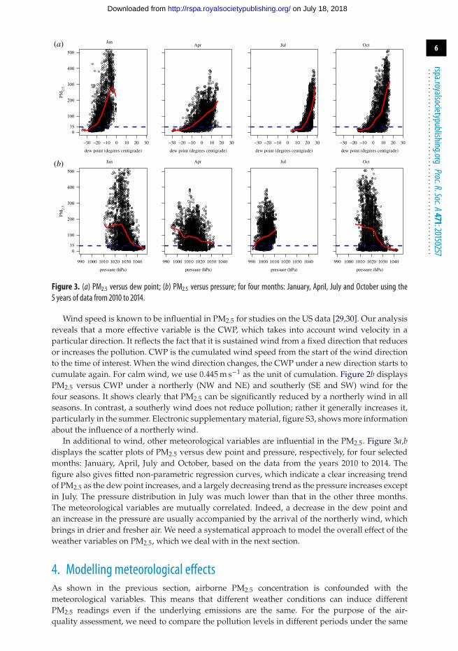
Figure 3. (a) PM2.5 versus dew point; (b) PM2.5 versus pressure; for four months: January, April, July and October using the5 years of data from 2010 to 2014.

Wind speed is known to be influential in PM2.5 for studies on the US data [29,30]. Our analysisreveals that a more effective variable is the CWP, which takes into account wind velocity in aparticular direction. It reflects the fact that it is sustained wind from a fixed direction that reducesor increases the pollution. CWP is the cumulated wind speed from the start of the wind directionto the time of interest. When the wind direction changes, the CWP under a new direction starts tocumulate again. For calm wind, we use 0.445 m s−1 as the unit of cumulation. Figure 2b displaysPM2.5 versus CWP under a northerly (NW and NE) and southerly (SE and SW) wind for thefour seasons. It shows clearly that PM2.5 can be significantly reduced by a northerly wind in allseasons. In contrast, a southerly wind does not reduce pollution; rather it generally increases it,particularly in the summer. Electronic supplementary material, figure S3, shows more informationabout the influence of a northerly wind.

In additional to wind, other meteorological variables are influential in the PM2.5. Figure 3a,bdisplays the scatter plots of PM2.5 versus dew point and pressure, respectively, for four selectedmonths: January, April, July and October, based on the data from the years 2010 to 2014. Thefigure also gives fitted non-parametric regression curves, which indicate a clear increasing trendof PM2.5 as the dew point increases, and a largely decreasing trend as the pressure increases exceptin July. The pressure distribution in July was much lower than that in the other three months.The meteorological variables are mutually correlated. Indeed, a decrease in the dew point andan increase in the pressure are usually accompanied by the arrival of the northerly wind, whichbrings in drier and fresher air. We need a systematical approach to model the overall effect of theweather variables on PM2.5, which we deal with in the next section.

4. Modelling meteorological effectsAs shown in the previous section, airborne PM2.5 concentration is confounded with themeteorological variables. This means that different weather conditions can induce differentPM2.5 readings even if the underlying emissions are the same. For the purpose of the air-quality assessment, we need to compare the pollution levels in different periods under the same



7


...................................................

meteorological conditions in order to be fair. However, the weather cannot be controlled. So,we must adjust for weather conditions. We are very much in the field of observational studies[31], where adjustment with respect to certain baseline variables is required in order to attain faircomparison on an outcome variable.

We provide a non-parametric framework for adjusting the mean and quantiles of the PM2.5distribution with respect to weather conditions in a period, say a month in a year, so that theadjusted means and quantiles of the same month in different years are comparable. The adjustedmeans and quantiles are needed to provide statistical evidence in order to assess if the pollutionis getting better or worse.

Let Yijt be the PM2.5 reading at an hour t in month j and year i, and Xijt be a vector consistingof air pressure (P), dew point (D), temperature (T), precipitation (Prec) and CWP (C) such thatXijt = (Pijt, Tijt, Dijt, Precijt, Cijt). Prec refers to the cumulative rain or snow hours according to theweather description from BCIA data. Relative humidity is not included as it can be determined bytemperature and dew point according to a physical relationship [32]. We denote wind direction asWijt such that Wijt = 1, 2, 3, 4 for NW, NE, S and CV, respectively, after merging SE and SW windswith the southern wind (S).

Let Uijt be the emission in the area that contains the site. One may use energy consumption asa proxy for Uijt. However, as there are only monthly energy consumption statistics at the nationallevel in China, and those at the provincial level are annual only, we have to treat Uijt as a latentvariable.

An underlying non-parametric regression model [33] for month j of year i is

Yijt = mij(Xijt, Wijt, Uijt) + εijt, t = 1, . . . , nij, (4.1)

where mij(x, w, u) = E(Yijt|Xijt = x, Wijt = w, Uijt = u) is the regression function, εijt is the residualthat satisfies E(εijt|Xijt, Wijt, Uijt) = 0, and nij is the number of observations in month j of year i.The residuals {εijt} are assumed to be stationary and weakly dependent [34] to reflect the dynamicnature of PM2.5 data.

As Uijt is latent, we consider a reduced model of (4.1)

Yijt = mij(Xijt, Wijt) + eijt, t = 1, . . . , nij, (4.2)

where mij(x, w) = E(Yijt|Xijt = x, Wijt = w) is the regression function based on the meteorologicalvariables only, and {eijt} are stationary and weakly dependent residuals. The electronicsupplementary material reports diagnostic tests on the stationarity and weakly dependentassumptions of {eijt} based on the fitted residuals of model (4.2), which shows adequate supportfor the assumptions.

An auto-regressive alteration of model (4.2) that better captures the dynamic of PM2.5 is

Yijt = βYij,t−1 + gij(Xijt, Wijt) + ηijt, (4.3)

where ηijt is stationary and weakly dependent such that E(ηijt|Yij,t−1, Xijt, Wijt) = 0 andgij(Xijt, Wijt) is the non-parametric part of the model. This model is useful in developingdetailed forecasting models for PM2.5, but not so much for the adjustment with respect to themeteorological variables. The latter is the main purpose of this paper.

In the above three models, we do not assume specific parametric forms for the regressionfunctions with respect to the meteorological variables, but want to learn from data non-parametrically. There are more than 700 hourly observations in each month (except February) for5 years, which are sufficient for carrying out the statistical learning. The monthly time span allowsenough data in the analysis under a comparable meteorological regime, especially with respect tothe temperature and dew point. Longer than a month may introduce excessive heterogeneity inthe weather conditions, and shorter than a month may have problems with a small sample sizeleading to unreliable estimates.

There may be a daily cycle of PM2.5 concentration, not accounted for in the above models.Temperature may be viewed as a proxy for daily variation in PM2.5, as well as for daily patterns



8


...................................................

in the boundary layer height (BLH), another variable that can influence the PM2.5 density. BLHdata are not available, although there are re-assimilated BLH values every 6 h in quite sparselydistributed grid points. Our analysis on the residuals did not reveal any daily or weekly cycles.

For the purpose of adjusting the PM2.5 distribution with respect to the meteorologicalcondition, we will concentrate on model (4.2). We consider a kernel smoothing estimatorfor mij(x, w) = E(Yijt|Xijt = x, Wijt = w) at each given wind direction w. Specifically, we use theNadaraya–Watson kernel estimator (NP) [33]:

mij(x, w) =∑nij

t=1 Kh(x − Xijt)YijtI(Wijt = w)∑nij

t=1 Kh(x − Xijt)I(Wijt = w), (4.4)

where I(Wijt = w) is the indicator function for a wind direction, Kh(z) = (K(z1/h1) · · · K(zq/hq)/h1 h2 · · · hq) is a product kernel generated by a univariate kernel function K(·) and q is thedimension of continuous variable Xijt. The smoothing bandwidths are h1, . . . , hq. Throughout thepaper, the Gaussian kernel K(u) = (2π )−1/2 exp(−u2/2) is used. The bandwidths reflect differentscales in the meteorological variables which contribute to the response. The local linear kernelestimator [35] can be employed as well, without changing the methodology proposed. We usecross-validation [33] to find suitable smoothing bandwidths.

The partially linear model (4.3) can be estimated using a combination of kernel smoothingand least-squares regression, where the smoothing bandwidths can be obtained by a version ofcross-validation (see [36] for details).

Table 1 reports the monthly RMSEs obtained by fitting models (4.2) and (4.3) to each monthlysample. It also reports the raw standard deviation of PM2.5 for each month. The table showsa huge reduction in the raw RMSE by fitting the non-parametric model (4.2). The averagepercentage of reduction for the 60 months was 78.2% with a standard deviation of 8.3%. Thepartially linear model (4.3) further reduced the RMSE of (4.2) by an average of 45.8% with astandard deviation 16.5%.

For the desired adjustment to the mean and the quantiles of the PM2.5 distribution, model (4.2)is more useful than the auto-regressive partially linear model (4.3). The latter is needed whenbuilding more specific models for forecasting the PM2.5 level. The rationale in presenting model(4.3) and its fitting results is to show that adding the auto-regressive part can improve the fit tothe data.

The bandwidths obtained by the cross-validation for each monthly model (4.2) containinformation on the importance of variables in explaining the PM2.5 concentration. If a covariateis redundant, the bandwidth selected by the cross-validation will diverge to the upper bound ofthe allowable range with probability tending to 1 (see [37] for details). As all the meteorologicalvariables, except the wind direction, are continuous, the upper bound is infinity.

We checked on the cross-validation bandwidths selected under each of the four winddirections (NW, NE, S and CV) for each month and employed 15 000 as the threshold to judgewhether a variable is redundant or not. The use of 15 000 was made by the observation that theCV bandwidths were either small, in the range of 0.2–100 (mostly from 0.2 to 10), or above 15 000.The electronic supplementary material, figure S4, reports the frequency of each variable whichwas selected for being useful among the 60 months under each wind direction. It shows that dewpoint and pressure were the most influential, followed by temperature and CWP. Rain and snowwere significant in the summer and winter, respectively. It is not surprising to see that CWP wasless influential under the CV (calm and variable wind) than the other wind directions, as it is hardto cumulate for this wind type.

There are six covariates in model (4.2). As rightly raised by a referee, the curse of dimensionalitymay be encountered in the kernel estimation of the regression surface, despite having around 720observations per month. We have tried to develop more specific parametric or semi-parametricmodels than (4.2) for the relationship between PM2.5 readings and the meteorological variables.However, it is quite challenging to obtain the relationship, as PM2.5 values are highly dependenton the wind direction and are highly nonlinear with respect to the meteorological variables, and



9


...................................................

Table 1. RMSEs by fitting the non-parametric regression (NP) model (4.2) and the partially linear regression (PL) model (4.3),for each month in 2010–2014. The standard deviation without any models for the monthly samples is reported in the columnsheaded ‘raw’.

(a)2010 2011 2012

month raw NP PL raw NP PL raw NP PL

1 93.94 10.07 5.42 46.31 8.26 7.42 131.47 8.44 7.31. . . . . . . . . . . . . . . . . . . . . . . . . . . . . . . . . . . . . . . . . . . . . . . . . . . . . . . . . . . . . . . . . . . . . . . . . . . . . . . . . . . . . . . . . . . . . . . . . . . . . . . . . . . . . . . . . . . . . . . . . . . . . . . . . . . . . . . . . . . . . . . . . . . . . . . . . . . . . . . . . . . . . . . . . . . . . . . . . . . . . . . . . . . . . . . . . . . . . . . . . .

2 84.83 34.86 26.47 143.18 24.50 10.67 78.39 13.22 5.81. . . . . . . . . . . . . . . . . . . . . . . . . . . . . . . . . . . . . . . . . . . . . . . . . . . . . . . . . . . . . . . . . . . . . . . . . . . . . . . . . . . . . . . . . . . . . . . . . . . . . . . . . . . . . . . . . . . . . . . . . . . . . . . . . . . . . . . . . . . . . . . . . . . . . . . . . . . . . . . . . . . . . . . . . . . . . . . . . . . . . . . . . . . . . . . . . . . . . . . . . .

3 84.29 13.58 6.91 73.74 8.02 6.10 86.69 14.41 10.43. . . . . . . . . . . . . . . . . . . . . . . . . . . . . . . . . . . . . . . . . . . . . . . . . . . . . . . . . . . . . . . . . . . . . . . . . . . . . . . . . . . . . . . . . . . . . . . . . . . . . . . . . . . . . . . . . . . . . . . . . . . . . . . . . . . . . . . . . . . . . . . . . . . . . . . . . . . . . . . . . . . . . . . . . . . . . . . . . . . . . . . . . . . . . . . . . . . . . . . . . .

4 73.52 4.55 2.92 67.01 11.17 13.41 69.12 11.36 5.83. . . . . . . . . . . . . . . . . . . . . . . . . . . . . . . . . . . . . . . . . . . . . . . . . . . . . . . . . . . . . . . . . . . . . . . . . . . . . . . . . . . . . . . . . . . . . . . . . . . . . . . . . . . . . . . . . . . . . . . . . . . . . . . . . . . . . . . . . . . . . . . . . . . . . . . . . . . . . . . . . . . . . . . . . . . . . . . . . . . . . . . . . . . . . . . . . . . . . . . . . .

5 59.04 10.86 6.97 51.59 6.94 8.30 56.00 20.13 14.70. . . . . . . . . . . . . . . . . . . . . . . . . . . . . . . . . . . . . . . . . . . . . . . . . . . . . . . . . . . . . . . . . . . . . . . . . . . . . . . . . . . . . . . . . . . . . . . . . . . . . . . . . . . . . . . . . . . . . . . . . . . . . . . . . . . . . . . . . . . . . . . . . . . . . . . . . . . . . . . . . . . . . . . . . . . . . . . . . . . . . . . . . . . . . . . . . . . . . . . . . .

6 52.26 11.00 9.36 76.05 20.15 10.24 68.50 15.48 8.51. . . . . . . . . . . . . . . . . . . . . . . . . . . . . . . . . . . . . . . . . . . . . . . . . . . . . . . . . . . . . . . . . . . . . . . . . . . . . . . . . . . . . . . . . . . . . . . . . . . . . . . . . . . . . . . . . . . . . . . . . . . . . . . . . . . . . . . . . . . . . . . . . . . . . . . . . . . . . . . . . . . . . . . . . . . . . . . . . . . . . . . . . . . . . . . . . . . . . . . . . .

7 72.49 16.00 10.39 80.13 16.99 8.74 56.67 16.84 6.58. . . . . . . . . . . . . . . . . . . . . . . . . . . . . . . . . . . . . . . . . . . . . . . . . . . . . . . . . . . . . . . . . . . . . . . . . . . . . . . . . . . . . . . . . . . . . . . . . . . . . . . . . . . . . . . . . . . . . . . . . . . . . . . . . . . . . . . . . . . . . . . . . . . . . . . . . . . . . . . . . . . . . . . . . . . . . . . . . . . . . . . . . . . . . . . . . . . . . . . . . .

8 67.32 9.90 8.01 54.27 21.48 8.40 59.20 21.19 4.63. . . . . . . . . . . . . . . . . . . . . . . . . . . . . . . . . . . . . . . . . . . . . . . . . . . . . . . . . . . . . . . . . . . . . . . . . . . . . . . . . . . . . . . . . . . . . . . . . . . . . . . . . . . . . . . . . . . . . . . . . . . . . . . . . . . . . . . . . . . . . . . . . . . . . . . . . . . . . . . . . . . . . . . . . . . . . . . . . . . . . . . . . . . . . . . . . . . . . . . . . .

9 78.43 28.44 12.57 85.13 26.36 8.24 52.43 11.70 5.13. . . . . . . . . . . . . . . . . . . . . . . . . . . . . . . . . . . . . . . . . . . . . . . . . . . . . . . . . . . . . . . . . . . . . . . . . . . . . . . . . . . . . . . . . . . . . . . . . . . . . . . . . . . . . . . . . . . . . . . . . . . . . . . . . . . . . . . . . . . . . . . . . . . . . . . . . . . . . . . . . . . . . . . . . . . . . . . . . . . . . . . . . . . . . . . . . . . . . . . . . .

10 124.59 21.45 11.05 122.91 20.37 10.49 92.44 30.96 11.40. . . . . . . . . . . . . . . . . . . . . . . . . . . . . . . . . . . . . . . . . . . . . . . . . . . . . . . . . . . . . . . . . . . . . . . . . . . . . . . . . . . . . . . . . . . . . . . . . . . . . . . . . . . . . . . . . . . . . . . . . . . . . . . . . . . . . . . . . . . . . . . . . . . . . . . . . . . . . . . . . . . . . . . . . . . . . . . . . . . . . . . . . . . . . . . . . . . . . . . . . .

11 133.69 41.00 9.33 89.62 25.35 13.65 85.21 30.38 12.05. . . . . . . . . . . . . . . . . . . . . . . . . . . . . . . . . . . . . . . . . . . . . . . . . . . . . . . . . . . . . . . . . . . . . . . . . . . . . . . . . . . . . . . . . . . . . . . . . . . . . . . . . . . . . . . . . . . . . . . . . . . . . . . . . . . . . . . . . . . . . . . . . . . . . . . . . . . . . . . . . . . . . . . . . . . . . . . . . . . . . . . . . . . . . . . . . . . . . . . . . .

12 114.89 23.83 11.69 107.23 11.85 8.90 96.97 5.81 5.84. . . . . . . . . . . . . . . . . . . . . . . . . . . . . . . . . . . . . . . . . . . . . . . . . . . . . . . . . . . . . . . . . . . . . . . . . . . . . . . . . . . . . . . . . . . . . . . . . . . . . . . . . . . . . . . . . . . . . . . . . . . . . . . . . . . . . . . . . . . . . . . . . . . . . . . . . . . . . . . . . . . . . . . . . . . . . . . . . . . . . . . . . . . . . . . . . . . . . . . . . .

(b)2013 2014

month raw NP PL raw NP PL

1 168.95 36.74 16.50 110.98 26.34 17.05. . . . . . . . . . . . . . . . . . . . . . . . . . . . . . . . . . . . . . . . . . . . . . . . . . . . . . . . . . . . . . . . . . . . . . . . . . . . . . . . . . . . . . . . . . . . . . . . . . . . . . . . . . . . . . . . . . . . . . . . . . . . . . . . . . . . . . . . . . . . . . . . . . . . . . . . . . . . . . . . . . . . . . . . . . . . . . . . . . . . . . . . . . . . . . . . . . . . . . . . . .

2 117.27 25.44 15.33 145.35 14.83 8.94. . . . . . . . . . . . . . . . . . . . . . . . . . . . . . . . . . . . . . . . . . . . . . . . . . . . . . . . . . . . . . . . . . . . . . . . . . . . . . . . . . . . . . . . . . . . . . . . . . . . . . . . . . . . . . . . . . . . . . . . . . . . . . . . . . . . . . . . . . . . . . . . . . . . . . . . . . . . . . . . . . . . . . . . . . . . . . . . . . . . . . . . . . . . . . . . . . . . . . . . . .

3 104.80 16.26 7.40 97.73 9.44 4.09. . . . . . . . . . . . . . . . . . . . . . . . . . . . . . . . . . . . . . . . . . . . . . . . . . . . . . . . . . . . . . . . . . . . . . . . . . . . . . . . . . . . . . . . . . . . . . . . . . . . . . . . . . . . . . . . . . . . . . . . . . . . . . . . . . . . . . . . . . . . . . . . . . . . . . . . . . . . . . . . . . . . . . . . . . . . . . . . . . . . . . . . . . . . . . . . . . . . . . . . . .

4 58.60 6.24 5.59 57.58 13.67 6.29. . . . . . . . . . . . . . . . . . . . . . . . . . . . . . . . . . . . . . . . . . . . . . . . . . . . . . . . . . . . . . . . . . . . . . . . . . . . . . . . . . . . . . . . . . . . . . . . . . . . . . . . . . . . . . . . . . . . . . . . . . . . . . . . . . . . . . . . . . . . . . . . . . . . . . . . . . . . . . . . . . . . . . . . . . . . . . . . . . . . . . . . . . . . . . . . . . . . . . . . . .

5 55.85 13.75 6.75 45.03 10.44 9.64. . . . . . . . . . . . . . . . . . . . . . . . . . . . . . . . . . . . . . . . . . . . . . . . . . . . . . . . . . . . . . . . . . . . . . . . . . . . . . . . . . . . . . . . . . . . . . . . . . . . . . . . . . . . . . . . . . . . . . . . . . . . . . . . . . . . . . . . . . . . . . . . . . . . . . . . . . . . . . . . . . . . . . . . . . . . . . . . . . . . . . . . . . . . . . . . . . . . . . . . . .

6 68.76 16.37 8.04 41.81 9.64 6.10. . . . . . . . . . . . . . . . . . . . . . . . . . . . . . . . . . . . . . . . . . . . . . . . . . . . . . . . . . . . . . . . . . . . . . . . . . . . . . . . . . . . . . . . . . . . . . . . . . . . . . . . . . . . . . . . . . . . . . . . . . . . . . . . . . . . . . . . . . . . . . . . . . . . . . . . . . . . . . . . . . . . . . . . . . . . . . . . . . . . . . . . . . . . . . . . . . . . . . . . . .

7 43.67 11.89 5.07 65.05 13.76 6.15. . . . . . . . . . . . . . . . . . . . . . . . . . . . . . . . . . . . . . . . . . . . . . . . . . . . . . . . . . . . . . . . . . . . . . . . . . . . . . . . . . . . . . . . . . . . . . . . . . . . . . . . . . . . . . . . . . . . . . . . . . . . . . . . . . . . . . . . . . . . . . . . . . . . . . . . . . . . . . . . . . . . . . . . . . . . . . . . . . . . . . . . . . . . . . . . . . . . . . . . . .

8 40.59 9.11 5.78 44.48 14.31 8.56. . . . . . . . . . . . . . . . . . . . . . . . . . . . . . . . . . . . . . . . . . . . . . . . . . . . . . . . . . . . . . . . . . . . . . . . . . . . . . . . . . . . . . . . . . . . . . . . . . . . . . . . . . . . . . . . . . . . . . . . . . . . . . . . . . . . . . . . . . . . . . . . . . . . . . . . . . . . . . . . . . . . . . . . . . . . . . . . . . . . . . . . . . . . . . . . . . . . . . . . . .

9 65.11 21.38 11.22 47.83 10.74 5.73. . . . . . . . . . . . . . . . . . . . . . . . . . . . . . . . . . . . . . . . . . . . . . . . . . . . . . . . . . . . . . . . . . . . . . . . . . . . . . . . . . . . . . . . . . . . . . . . . . . . . . . . . . . . . . . . . . . . . . . . . . . . . . . . . . . . . . . . . . . . . . . . . . . . . . . . . . . . . . . . . . . . . . . . . . . . . . . . . . . . . . . . . . . . . . . . . . . . . . . . . .

10 95.05 20.41 8.53 118.08 28.11 6.58. . . . . . . . . . . . . . . . . . . . . . . . . . . . . . . . . . . . . . . . . . . . . . . . . . . . . . . . . . . . . . . . . . . . . . . . . . . . . . . . . . . . . . . . . . . . . . . . . . . . . . . . . . . . . . . . . . . . . . . . . . . . . . . . . . . . . . . . . . . . . . . . . . . . . . . . . . . . . . . . . . . . . . . . . . . . . . . . . . . . . . . . . . . . . . . . . . . . . . . . . .

11 92.56 19.41 10.38 109.71 23.78 11.12. . . . . . . . . . . . . . . . . . . . . . . . . . . . . . . . . . . . . . . . . . . . . . . . . . . . . . . . . . . . . . . . . . . . . . . . . . . . . . . . . . . . . . . . . . . . . . . . . . . . . . . . . . . . . . . . . . . . . . . . . . . . . . . . . . . . . . . . . . . . . . . . . . . . . . . . . . . . . . . . . . . . . . . . . . . . . . . . . . . . . . . . . . . . . . . . . . . . . . . . . .

12 107.36 22.72 15.93 93.88 23.18 12.16. . . . . . . . . . . . . . . . . . . . . . . . . . . . . . . . . . . . . . . . . . . . . . . . . . . . . . . . . . . . . . . . . . . . . . . . . . . . . . . . . . . . . . . . . . . . . . . . . . . . . . . . . . . . . . . . . . . . . . . . . . . . . . . . . . . . . . . . . . . . . . . . . . . . . . . . . . . . . . . . . . . . . . . . . . . . . . . . . . . . . . . . . . . . . . . . . . . . . . . . . .

there is significant confounding among the covariates too. We note that, for the purpose of the airquality assessment, a parametric or semi-parametric model may not be necessary, as the ultimatepurpose of the kernel smoothing is to obtain the adjusted means and quantiles rather than theregression function. Hence, the kernel smoothing and the associated curse of dimensionality willhave fewer effects on the inference of the adjusted means and quantiles. Having said the above,the non-parametric model (4.2) should be viewed as the first step in our model building exerciseas it provides a benchmark for further development of more specific models. Linear or additivemodels based on functional principal component analysis [38,39] can be applied to reveal more



10


...................................................

explicit association between the PM2.5 process and meteorological covariates. The developmentof more interpretable models is an area of our future research.

5. Adjustment to meteorological conditionsAs a completely randomized experiment that controls the weather is not possible, the observedPM2.5 has to be adjusted with respect to the observed meteorological conditions.

We first present the adjustment to the monthly means of PM2.5 with respect to themeteorological conditions for the 5 years. Let f·j(x, w) be the joint density function of themeteorological variables (Xijt, Wijt) in month j of all years. The adjusted mean PM2.5 in monthj and year i is

μij =4∑

w=1

∫E(Yijt|Xijt = x, Wijt = w)f·j(x, w) dx

=4∑

w=1

∫mij(x, w)f·j(x, w) dx. (5.1)

Substituting the kernel estimator mij(x, w) given in (4.4), the estimator of the adjusted mean is

μij =⎛⎝ n.j∑

a=1

naj

⎞⎠

−1 n.j∑a=1

naj∑t=1

4∑w=1

mij(Xajt, Wajt)I(Wajt = w), (5.2)

where n.j is the number of years that month j is observed, which is 5 for our analysis. It can beshown that μij is a consistent and asymptotically unbiased estimator of the true μij, using a similartechnique to [40].

The essence of the adjustment is to use the data in the jth month of year i to estimate theregression function mij, and then substitute the meteorological information of all 5 years for monthj to obtain the estimator of μij, as suggested by (5.2). This is the approach used in observationalstudies [31] for carrying out adjustment based on covariates to a response so as to remove the biasdue to a lack of randomness in the study.

As the observed data are dependent time series, the block bootstrap method [41] is needed toestimate the variance of μij. The block bootstrap resamples blocks of observations to retain thedependence in the original data series. For each month j in year i, let Zt = (Xijt, Wijt), t = 1, . . . , T =nij. We considered moving blocks with length l: B1 = (Z1, . . . , Zl), . . . , BT−l+1 = (ZT−l+1, . . . , ZT),BT−l+2 = (ZT−l+2, . . . , ZT, Z1), . . . , BT = (ZT, Z1, . . . , Zl−1). The wrapping at the boundary ensuresthat each of the original observations appears with equal chance in a bootstrapped sample. Thenwe independently resampled T/l blocks from a total of T blocks, which were joined together toform a resampled monthly times series {Xb

ijt, Wbijt} for the bth replication of month j in year i.

Based on the resampled weather variables {(Xbijt, Wb

ijt)}, we impute the corresponding PM2.5

via an estimated model (4.2): Yb∗ijt = mij(Xb

ijt, Wbijt) + εb∗

ijt , where εb∗ijt is resampled from a two-point

distribution [42],

εb∗ijt =

⎧⎪⎪⎪⎨⎪⎪⎪⎩

ε(Xbijt, Wb

ijt)1 − √

52

with probability1 + √

5

2√

5

ε(Xbijt, Wb

ijt)1 + √

52

with probability 1 − 1 + √5

2√

5,

(5.3)

and ε(Xbijt, Wb

ijt) is a residual estimator via a kernel smoothing of ε2ijt = {Yijt − mij(Xijt, Wijt)}2

ε2(x, w) =∑nij

t=1 Kh(x − Xijt)ε2ijtI(Wijt = w)∑nij

t=1 Kh(x − Xijt)I(Wijt = w). (5.4)



11


...................................................

Matching the resampled meteorological data and the imputed PM2.5 gives us the bootstrapresampled data series {(Yb∗

ijt , Xbijt, Wb

ijt)} for i = 1, . . . , 5, t = 1, . . . , nij. We re-estimate the regression

function to obtain mbij(x, w) by (4.4), which then gives rise to the adjusted mean for the bth

bootstrap replication

μbij =

⎛⎝ n.j∑

a=1

naj

⎞⎠

−1 n.j∑a=1

naj∑t=1

4∑w=1

mbij(X

bajt, Wb

ajt)I(Wbajt = w). (5.5)

The bootstrap estimate of the standard deviation of μij is

σij =√∑B

b=1(μbij − μij)2

B − 1. (5.6)

Similarly to the adjusted mean in (5.1), we define the adjusted distribution function of PM2.5for month j of year i as

Gij(y) =4∑

w=1

∫Fij(y|x, w)f·j(x, w) dx,

where Fij(y|x, w) = E(I{Yijt ≤ y}|Xijt = x, Wijt = w) is the conditional distribution and I{Yijt ≤ y} isthe indicator function. In order to estimate Gij(y), we first estimate Fij(y|x, w) by the kernelsmoothing method under each wind direction:

Fij(y|x, w) =∑nij

t=1 Kh(x − Xijt)I(Wijt = w)Gh0 (Yijt − y)∑nij

t=1 Kh(x − Xijt)I(Wijt = w),

where Gh0 (x) = ∫x/h0−∞ K(u) d u is the integration of the univariate kernel K. Then, we estimate

Gij(y) by

Gij(y) =⎛⎝ n·j∑

a=1

naj

⎞⎠

−1 n·j∑a=1

naj∑t=1

4∑w=1

Fij(y|Xajt, Wajt)I(Wajt = w).

For any q ∈ (0, 1), the adjusted qth percentile is estimated by G−1ij (q). The standard error of

the estimated percentiles can be obtained by mimicking the block bootstrap procedure for theadjusted mean.

Let us consider how to measure the effect of emissions by revisiting model (4.1). Suppose thatthe regression function in (4.1) is additive with respect to the meteorological variable (Xijt, Wijt)and the emission level Uijt, such that

Yijt = mij,1(Xijt, Wijt) + mij,2(Uijt) + εijt.

If the emission Uijt is independent of weather conditions (Xijt, Wijt), it can be shown that

mij(x, w) = E(Yijt|Xijt = x, Wijt = w) = mij,1(x, w) + E{mij,2(Uijt)}and the adjusted mean in (5.1) can be written as

μij =4∑

w=1

∫E(Yijt|Xijt = x, Wijt = w)f·j(x, w) dx

=4∑

w=1

∫mij,1(x, w)f·j(x, w) dx + E{mij,2(Uijt)}. (5.7)

The result in (5.7) implies that, under the additive and independence assumptions, theadjusted average PM2.5 is the sum of two terms: one due to weather conditions and the otherdue to emissions. This may be used to obtain the effect of emission by taking the difference in μij.For instance, if the weather impact in January is the same among all the years considered, thenμi,1 − μj,1 will reflect the different emission levels between years i and j on PM2.5. Likewise, if the



12


...................................................

weather impacts between two neighbouring time periods are roughly the same, the differencein the adjustment means informs the difference in the effects of emissions between the twoperiods. The latter approach is used in our studies on the impacts of the emission control forthe Asia-Pacific Economic Cooperation (APEC) meeting and winter heating in §7.

We note here that the emission level Uijt does not measure aerosol abundance, but the originalemission level directly related to energy consumption, as otherwise the assumption of it beingindependent of the meteorological variable would be unreasonable, as secondary aerosols areimpacted by weather conditions. Of course, the independent assumption does not hold in a longertime scale, as the emission level has an annual cycle. However, for the monthly time frame thatwe are considering the assumption is reasonable.

6. Five-year assessmentWe applied the adjustment on the mean and the quantiles of the PM2.5 with respect to themeteorological variables outlined in the previous section to the 60 months in the years 2010–2014. Figure 4a presents the monthly adjusted and raw averages of PM2.5, along with 95%confidence intervals for the adjusted means based on the standard errors obtained via the blockbootstrap with block size l = 12 h. The confidence intervals were obtained by extending 1.96 timesthe standard deviation above and below the adjusted mean. We observe substantial differencesbetween the adjusted and the raw averages. Among the 60 months in the 5 years, 28 months hadraw averages outside the intervals. This demonstrates that it is necessary to adjust the averagesas those without any adjustments would be unfairly impacted by the weather.

As more robust alternatives to the mean, figure 4b gives the adjusted percentiles of monthlyPM2.5 at 90th, 75th, 50th (median), 25th and 10th percentiles, along with their 95% CI obtainedvia the block bootstrap method with l = 12. It is observed that there were much smaller monthlyvariations for the three lower percentiles. The variation increased in the two higher percentiles.We find that the medians were significantly above the threshold 35 µg m−3 in 56 months and weremostly ranged between 70 and 100 µg m−3.

The monthly 75th percentiles were significantly higher than 90 µg m−3 in all but three months.The pattern displayed by the 90th and 75th percentiles showed a much higher level of PM2.5pollution from October to March. This reflects the extra emissions due to the winter heatingseason in North China from November to March [16], and the biomass burning by farmers inOctober [13]. There are also increased mineral aerosols due to transported dust in winter andspring [43].

The State Council of China set PM2.5 reduction targets for various regions of China in October2013. Those for Beijing and NCP are (i) a 25% reduction by 2017 from the 2012 level and (ii) anannual average PM2.5 in Beijing below 60 µg m−3.

To check on progress towards the reduction targets, figure 5 gives the differences in adjustedaverages, medians and 90th percentiles between 2013 and 2012 and between 2014 and 2012. Theexact numerical values are given in the electronic supplementary material, table S1. Figure 5reveals that the reduction in the average PM2.5 from 2012 happened in two months in 2013, andonly one of them (August) was significant at 2.5% (p < 0.025). Six months in 2014 had reductionsin averages over 2012, and only two of them (May and June) were significant at 2.5%. In contrast,among the 10 months in 2013 which had increased averages over their 2012 counterparts, fourmonths’ increases were significant at 2.5%. In 2014, among the six months with higher averages,four of them were significantly higher than their counterparts in 2012 at 2.5%. We note that mostof the increases in 2013 and 2014 were much larger in magnitude than most of the decreases inthe 2 years.

The situation for the medians was similar to that of the averages reported above. Only twomonths in 2014 had a significantly smaller median than 2012, and five months had a significantlylarger median at 2.5% significance. In 2013, there was no significant reduction, whereas significantincreases happened in two months. There were improvements about the 90th percentiles in threemonths in year 2014 and one month in 2013. However, significant increases in the 90th percentiles



13


...................................................

500

300

100

0

500

300

100

02 4 6 8 10 12

month2 4 6 8 10 12

month

2013 2014

(a) 2010

2 4 6 8 10 12month

2 4 6 8 10 12month

2 4 6 8 10 12month

2 4 6 8 10 12month

2 4 6 8 10 12month

200

PM2.

5PM

2.5

PM2.

5PM

2.5

150

100

50

200

150

100

50

2011

2013 2014

2012

2010

2 4 6 8 10 12month

2 4 6 8 10 12month

2 4 6 8 10 12

90%75%50%25%10%PM2.5 = 35

month

2011 2012(b)

Figure 4. Adjusted average and percentiles of PM2.5. (a) The adjustedmonthly averages (solid lines) and raw averages (dashedlines). (b) The adjusted monthly 90th (purple), 75th (brown), 50th (median, red), 25th (yellow) and 10th (green) percentiles ofPM2.5 concentration with the black dashed line of PM2.5 = 35µg m−3. The bars are 1.96 times the standard deviations aboveand below the estimates.

happened in four months in both 2013 and 2014. Moreover, the adjusted annual averages(standard error) from 2010 to 2014 were 101.3 µg m−3 (1.99), 97.6 µg m−3 (2.08), 91.5 µg m−3 (1.72),101.2 µg m−3 (1.85) and 96.9 µg m−3 (2.09), respectively, indicating that the PM2.5 pollution inBeijing has actually got worse since 2012. The electronic supplementary material, table S2, givesthe annual adjusted means and percentiles and their standard errors. The percentiles in 2013 and2014 were all significantly higher than their 2012 counterparts except the 10th percentile in 2014,lending support to the above conclusion based on the averages.



14


...................................................

(a)

2013 – 2012 2014 − 2012

–40–30–20–10

0102030405060

Jan Feb Mar Apr May Jun Jul Aug Sep Oct Nov Dec Jan Feb Mar Apr May Jun Jul Aug Sep Oct Nov Dec

diff

eren

ce

significant increase insignificant increase insignificant reduction significant reduction

(b)2013 – 2012 2014 – 2012

–50–40–30–20–10

010203040506070


diff

eren

ce

significant increase insignificant increase insignificant reduction significant reduction indifference

–150–100–50

050

100150

diff

eren

ce

2013 – 2012 2014 – 2012


significant increase insignificant increase insignificant reduction significant reduction

(c)

Figure 5. Differences in PM2.5 between 2013 and 2012, and between 2014 and 2012. (a) Differences in the adjusted averages.(b) Differences in the adjusted medians. (c) Differences in the adjusted 90th percentiles. ‘Difference’ means the 2013/2014 valueof a month minus the 2012 value of the same month. The boxes are 1.96 times the standard deviations above and below thedifferences (white line). Significant increases (decreases) correspond to boxes which are entirely above (below) the horizontalline of zero; and insignificant increases (decreases) correspond to boxeswhich intercept the horizontal line. A significant increase(reduction) means the p-value is less than 0.025 for the one-sided test for the difference being positive (negative).

7. Two quasi-experimentsQEs [26,44] may be used in conjunction with observational studies to gauge the effect of theemissions Uijt, information about which is not available. We have two opportunities for QEs. Onewas the 2014 APEC meeting in Beijing on 8–11 November. The second QE is the annual winterheating season which runs usually from 15 November to 15 March in Beijing and the NCP. Thesetwo experiments offer opportunities to assess the impacts of emissions on PM2.5 and providepotential policy options to combat the pollution.

To ensure the air quality for the APEC meeting, the Chinese government had ordered atemporary closure of factories in Beijing and the northern part of the NCP from 3 to 12 November,with half of the cars in Beijing being ordered to stay off the roads according to the last digit of thelicence plate being even or odd. From 6 to 12 November, the control zone was enlarged to include



15


...................................................

220

406080

100120140160180200

(a)

0

2010 2011 2012

3–12 Nov 6–12 Nov

2013 2014 2010 2011 2012 2013 2014

20

40

60

80

100

120

140

0

20

40

60

80

100

120

140PM

2.5

PM2.

5

(c)

non-heating heating

2010 2011 2012 2013 2014

non-heating heating

2010 2011 2012 2013 2014

60

80

100

120

140

160

PM2.

5

(b)

Figure 6. Adjusted averages in the QEs. (a) Adjusted averages in the periods of APEC. (b) Adjusted averages in the non-heatingand heating periods in November. (c) Adjusted averages in the non-heating and heating periods in March. The boxes are1.96 times the standard deviations above and below the estimates (white line). The black dots are the averages without theadjustment.

the entire NCP and part of the neighbouring Shanxi and Inner Mongolia provinces. Schoolsand public offices were closed in this second period until 12 November with much suppressedeconomic and social activities. To evaluate the impacts of the APEC measures on Beijing’s airquality, we conducted the proposed adjustment to the average PM2.5 levels for the two timeperiods, 3–12 November and 6–12 November, by considering the meteorological conditions overthe two periods in the 5 years from 2010 to 2014. The left panel of figure 6a shows that the 2014average in the first period of 3–12 November was significantly less than the averages in 2013 withthe p-value being almost zero. However, the reduction in 2014 was not statistically significant



16


...................................................

at the 5% level when compared with the 2010, 2011 and 2012 averages (the p-values were 0.28,0.61, 0.25, respectively). For the second period of 6–12 November (the right panel in figure 6a),the p-values for testing the adjusted mean in 2014 being less than the corresponding periods in2010–2013 were 0.06, 0.11, 0.07 and 0, respectively, which were much lower than those in the firstperiod. Although only the p-value when comparing with 2013 was significant at 5%, the p-valuesfor the other three years were only slightly higher than 0.05, which reflected the large variation inthe weather conditions. Thus, the administrative actions to enlarge the control zone on emissionsdid have some effect in reducing the PM2.5 level in the second period. The PM2.5 reductionwas averaged at 25.3% compared with the previous four years; see electronic supplementarymaterial, table S3, for detailed numerical values about the averages and percentiles. That theAPEC emission control measures were more effective in reducing the pollution in the secondtime period may be due to the fact that it takes time for the raw pollutants to become PM2.5 insecondary reactions.

For the second QE on the effect of heating, we chose the two weeks from the start of theheating date in November and the two weeks just prior to the termination of heating in Marchas the treatment periods. As controls (non-heating periods), we chose the two weeks just beforethe start of heating in November and the two weeks right after the end of heating in March. Theheating period can start earlier than 15 November or be extended after 15 March depending onthe temperature at that time. For instance, it was started on 3 November in 2012; and ended on22, 18, 17 March in 2010, 2012 and 2013, respectively. Figure 6b,c displays the pairwise adjustedaverages for the heating and non-heating periods in November and March, respectively, for thelast 5 years. The figures show startling increases in PM2.5 due to heating in both November andMarch, with the increases being highly statistically significant in all heating seasons (the p-valueswere all ≤ 0.015). The increases in November due to heating ranged from 31% (in 2013) to 183%(in 2010). The increase of 157% in 2014 was partly due to the APEC measures and should notbe taken as a norm. The reduction in March due to the cessation of heating ranged from 24% to42%. In other words, the increase due to heating in March ranged from 31% to 72%. The electronicsupplementary material, tables S4 and S5, gives the exact numeric values for the adjusted meansand percentiles for each heating and non-heating period, which strongly support heating havinga significant effect on PM2.5 in Beijing. The table also reports the original unadjusted averagesand percentiles for the heating treatment and the non-heating control. This shows that theeffect of heating would not have been revealed in many seasons if the adjustments were notcarried out.

8. Incorporating other chemicalsSo far our analysis is solely based on the dependence between PM2.5 and the meteorologicalvariables without considering the atmospheric chemical reaction that generates PM2.5. Asrightly pointed out by a referee, urban aerosol formation is significantly contributed to bysecondary formation processes as elaborated in [8]. To extend our analysis to include potentialsecondary formation, we face a hurdle in that the US Embassy only measures the PM2.5concentration without other chemical compounds. To get around the problem, we consider hourlyrecordings of three pollutants—SO2, NO2 and CO—at a neighbouring MEP site, Nongzhanguan,which is 1.2 km south of the embassy. Measurements of more extended chemical elements are notavailable in most of the MEP sites, except O3. Our preliminary analysis reveals that O3 has littleexplaining power for PM2.5. Hence, we did not include it in the analysis. Although the MEP siteat Nongzhanguan had started measuring PM2.5 and the chemical compounds in early 2013, thedata in 2013 suffered from a high percentage of missing values. Therefore, we only analysed the2014 data.

We consider adding a linear term for the three chemicals to the non-parametric model (4.2)and the auto-regressive model (4.3):

Yijt = β1SO2ijt + β2NO2ijt + β3COijt + mij(Xijt, Wijt) + eijt, t = 1, . . . , nij (8.1)



17


...................................................

Table 2. RMSEs by fitting the non-parametric model (4.2), the non-parametric auto-regressive model (4.3) and models (8.1)and (8.2) by adding a linear regressive part for the three chemicals, respectively, for each month in 2014. The column headed‘raw’ is the monthly sample standard deviation of PM2.5 without any model.

RMSE RMSE reduction (%)

year-month raw (4.2) (8.1) (4.3) (8.2) (4.2) (8.1) (4.3) (8.2)

2014-1 110.98 26.34 18.04 17.05 15.10 76.26 83.75 84.63 86.39. . . . . . . . . . . . . . . . . . . . . . . . . . . . . . . . . . . . . . . . . . . . . . . . . . . . . . . . . . . . . . . . . . . . . . . . . . . . . . . . . . . . . . . . . . . . . . . . . . . . . . . . . . . . . . . . . . . . . . . . . . . . . . . . . . . . . . . . . . . . . . . . . . . . . . . . . . . . . . . . . . . . . . . . . . . . . . . . . . . . . . . . . . . . . . . . . . . . . . . . . .

2014-2 145.35 14.83 12.16 8.94 7.78 89.80 91.63 93.85 94.65. . . . . . . . . . . . . . . . . . . . . . . . . . . . . . . . . . . . . . . . . . . . . . . . . . . . . . . . . . . . . . . . . . . . . . . . . . . . . . . . . . . . . . . . . . . . . . . . . . . . . . . . . . . . . . . . . . . . . . . . . . . . . . . . . . . . . . . . . . . . . . . . . . . . . . . . . . . . . . . . . . . . . . . . . . . . . . . . . . . . . . . . . . . . . . . . . . . . . . . . . .

2014-3 97.73 9.44 3.76 4.09 3.12 90.34 96.16 95.81 96.81. . . . . . . . . . . . . . . . . . . . . . . . . . . . . . . . . . . . . . . . . . . . . . . . . . . . . . . . . . . . . . . . . . . . . . . . . . . . . . . . . . . . . . . . . . . . . . . . . . . . . . . . . . . . . . . . . . . . . . . . . . . . . . . . . . . . . . . . . . . . . . . . . . . . . . . . . . . . . . . . . . . . . . . . . . . . . . . . . . . . . . . . . . . . . . . . . . . . . . . . . .

2014-4 57.58 13.67 6.50 6.29 5.01 76.26 88.71 89.08 91.30. . . . . . . . . . . . . . . . . . . . . . . . . . . . . . . . . . . . . . . . . . . . . . . . . . . . . . . . . . . . . . . . . . . . . . . . . . . . . . . . . . . . . . . . . . . . . . . . . . . . . . . . . . . . . . . . . . . . . . . . . . . . . . . . . . . . . . . . . . . . . . . . . . . . . . . . . . . . . . . . . . . . . . . . . . . . . . . . . . . . . . . . . . . . . . . . . . . . . . . . . .

2014-5 45.03 10.44 11.84 9.64 9.03 76.81 73.72 78.59 79.94. . . . . . . . . . . . . . . . . . . . . . . . . . . . . . . . . . . . . . . . . . . . . . . . . . . . . . . . . . . . . . . . . . . . . . . . . . . . . . . . . . . . . . . . . . . . . . . . . . . . . . . . . . . . . . . . . . . . . . . . . . . . . . . . . . . . . . . . . . . . . . . . . . . . . . . . . . . . . . . . . . . . . . . . . . . . . . . . . . . . . . . . . . . . . . . . . . . . . . . . . .

2014-6 41.81 9.64 7.95 6.10 4.97 76.95 80.99 85.41 88.10. . . . . . . . . . . . . . . . . . . . . . . . . . . . . . . . . . . . . . . . . . . . . . . . . . . . . . . . . . . . . . . . . . . . . . . . . . . . . . . . . . . . . . . . . . . . . . . . . . . . . . . . . . . . . . . . . . . . . . . . . . . . . . . . . . . . . . . . . . . . . . . . . . . . . . . . . . . . . . . . . . . . . . . . . . . . . . . . . . . . . . . . . . . . . . . . . . . . . . . . . .

2014-7 65.05 13.76 9.63 6.15 5.77 78.85 85.20 90.55 91.12. . . . . . . . . . . . . . . . . . . . . . . . . . . . . . . . . . . . . . . . . . . . . . . . . . . . . . . . . . . . . . . . . . . . . . . . . . . . . . . . . . . . . . . . . . . . . . . . . . . . . . . . . . . . . . . . . . . . . . . . . . . . . . . . . . . . . . . . . . . . . . . . . . . . . . . . . . . . . . . . . . . . . . . . . . . . . . . . . . . . . . . . . . . . . . . . . . . . . . . . . .

2014-8 44.48 14.31 9.01 8.56 7.43 67.84 79.74 80.76 83.29. . . . . . . . . . . . . . . . . . . . . . . . . . . . . . . . . . . . . . . . . . . . . . . . . . . . . . . . . . . . . . . . . . . . . . . . . . . . . . . . . . . . . . . . . . . . . . . . . . . . . . . . . . . . . . . . . . . . . . . . . . . . . . . . . . . . . . . . . . . . . . . . . . . . . . . . . . . . . . . . . . . . . . . . . . . . . . . . . . . . . . . . . . . . . . . . . . . . . . . . . .

2014-9 47.83 10.74 8.39 5.73 5.33 77.55 82.47 88.02 88.85. . . . . . . . . . . . . . . . . . . . . . . . . . . . . . . . . . . . . . . . . . . . . . . . . . . . . . . . . . . . . . . . . . . . . . . . . . . . . . . . . . . . . . . . . . . . . . . . . . . . . . . . . . . . . . . . . . . . . . . . . . . . . . . . . . . . . . . . . . . . . . . . . . . . . . . . . . . . . . . . . . . . . . . . . . . . . . . . . . . . . . . . . . . . . . . . . . . . . . . . . .

2014-10 118.08 28.11 13.13 6.58 5.56 76.20 88.88 94.43 95.29. . . . . . . . . . . . . . . . . . . . . . . . . . . . . . . . . . . . . . . . . . . . . . . . . . . . . . . . . . . . . . . . . . . . . . . . . . . . . . . . . . . . . . . . . . . . . . . . . . . . . . . . . . . . . . . . . . . . . . . . . . . . . . . . . . . . . . . . . . . . . . . . . . . . . . . . . . . . . . . . . . . . . . . . . . . . . . . . . . . . . . . . . . . . . . . . . . . . . . . . . .

2014-11 109.71 23.78 13.72 11.12 10.80 78.32 87.50 89.87 90.16. . . . . . . . . . . . . . . . . . . . . . . . . . . . . . . . . . . . . . . . . . . . . . . . . . . . . . . . . . . . . . . . . . . . . . . . . . . . . . . . . . . . . . . . . . . . . . . . . . . . . . . . . . . . . . . . . . . . . . . . . . . . . . . . . . . . . . . . . . . . . . . . . . . . . . . . . . . . . . . . . . . . . . . . . . . . . . . . . . . . . . . . . . . . . . . . . . . . . . . . . .

2014-12 93.88 23.18 11.76 12.16 10.34 75.31 87.47 87.05 88.99. . . . . . . . . . . . . . . . . . . . . . . . . . . . . . . . . . . . . . . . . . . . . . . . . . . . . . . . . . . . . . . . . . . . . . . . . . . . . . . . . . . . . . . . . . . . . . . . . . . . . . . . . . . . . . . . . . . . . . . . . . . . . . . . . . . . . . . . . . . . . . . . . . . . . . . . . . . . . . . . . . . . . . . . . . . . . . . . . . . . . . . . . . . . . . . . . . . . . . . . . .

average 81.46 16.52 10.49 8.53 7.52 78.37 85.52 88.17 89.57. . . . . . . . . . . . . . . . . . . . . . . . . . . . . . . . . . . . . . . . . . . . . . . . . . . . . . . . . . . . . . . . . . . . . . . . . . . . . . . . . . . . . . . . . . . . . . . . . . . . . . . . . . . . . . . . . . . . . . . . . . . . . . . . . . . . . . . . . . . . . . . . . . . . . . . . . . . . . . . . . . . . . . . . . . . . . . . . . . . . . . . . . . . . . . . . . . . . . . . . . .

and

Yijt = β0Yij,t−1 + β1SO2ijt + β2NO2ijt + β3COijt + gij(Xijt, Wijt) + ηijt. (8.2)

We use the parametric linear function to avoid further issues with the curse of dimensionality.Table 2 reports RMSEs for fitting models (4.2), (4.3), (8.1) and (8.2) and the percentages of

reduction in relative RMSEs of the four models. We do not report the R2-values of the modelsas they were all above 0.93, which can exaggerate the goodness-of-fit of models. The table showsthat the meteorological variables explained on average 78% of the uncertainty, as measured by theRMSEs, of the PM2.5 as secondary formation of PM2.5 requires certain meteorological conditions.The RMSEs were further reduced for models (8.1) and (8.2) of the order of 8–10%, indicating thatmore uncertainty was explained by incorporating the three chemicals. The relative amount ofreductions provides a measure of the uncertainty missed by considering only the meteorologicalvariables. In addition, the reductions from (4.3) to (8.2) were less than those from (4.2) to (8.1). Thiswas because the lagged PM2.5 term (the auto-regressive part) in (4.3) and (8.2) already containedinformation about the three chemicals.

The estimates of the regression coefficients of the three chemical elements together with their p-values [45] for being significantly different from zero are reported in the electronic supplementarymaterial, tables S6–S8. The results show that, for model (8.1), SO2 tended to be significant inthe winter months, and NO2 and CO were significant in almost all the months of the year. Thesignificance of SO2 in winter was likely to be due to the excessive coal burning for heating. Thesignificance of NO2 and CO for the whole year indicates that the pollution from motor vehiclesplays an important role in air pollution in Beijing, which cannot be captured fully by consideringmeteorological conditions alone. The fitting results for model (8.2) in the electronic supplementarymaterial, table S8, show that, when the lagged PM2.5 was added to the model, the three chemicalsbecame less significant, which was consistent with the findings in table 2.



18


...................................................

9. DiscussionBy employing statistical learning based on 5 years’ data, we propose a set of statistical measuresto quantify the severity of PM2.5 pollution in Beijing. We provide a methodological frameworkto produce adjusted means and percentiles for objectively comparing PM2.5 concentrations thatneutralize the impacts of meteorological conditions. The adjustment allows us to find significanteffects of the emission reduction measures for the APEC meeting and annual winter heating onthe PM2.5. Our analyses have the following conclusions and broad implications.

All our analyses point to a conclusion that, up to the end of 2014, the PM2.5 pollution in Beijinghad not improved over the 2012 levels, and the air quality had in fact got worse.

Our analysis of the effect of heating on PM2.5 reveals that winter heating contributessignificantly to PM2.5 abundance in Beijing. A step that various authorities in the NCP can take isto phase out the use of coal for heating and convert all the furnaces in cities and towns to naturalgas. However, this action (even though it may be perceived as too radical) alone is not enough foreliminating the pollution. To appreciate this point, we note from our analysis that the heating hascontributed a more than 50% increase (on average) in PM2.5 in the winter months in Beijing since2010. This means that one-third of the PM2.5 in the heating months is due to heating. This leadsto a best case scenario where using natural gas or other cleaner energy for heating in the NCP atbest reduces the average PM2.5 in the months of December, January and February by one-third.At the same time, we use the averages in the non-heating portion of November and March asthe monthly average while keeping the other months’ PM2.5 levels the same. Then, the annualaverages for 2013 and 2014 would be 88.2 µg m−3 and 80.1 µg m−3, respectively, which representonly 3.6% and 12.5% reductions, respectively, from the 2012 annual average of 91.5 µg m−3. Thesetwo numbers are still well short of the 25% reduction target of 68.6 µg m−3.

Despite the drastic APEC measures which basically shut down a significant portion of theeconomy in the NCP for 10 days, the average PM2.5 in the period 6–12 November 2014 was52.2 µg m−3 (6.72) (electronic supplementary material, table S3), which was still much higher thanthe healthy threshold of 35 µg m−3. This indicates that, under the existing energy consumptionprofile of the NCP, it is rather unlikely that Beijing will attain clean air of 35 µg m−3 or lower overa prolonged period. Hence, transitions to alternative forms of industrial installations with loweremission profiles must be taken in order for Beijing to attain the standard of healthy air.

Data accessibility. The data of PM2.5 at the US Embassy are from http://www.stateair.net/web/historical/1/1.html and the weather data are from http://weather.nocrew.org. The data of the chemical compounds inNongzhanguan can be acquired from http://air.epmap.org/.Authors’ contributions. S.X.C. led the project. X.L. performed most of the analyses assisted by T.Z., B.G., S.L., H.Z.,S.Z. and H.H.. T.Z. performed the tests on the residuals on models (4.2) and (4.3). S.X.C., H.H., X.L. and T.Zwrote the manuscript with inputs from the others. All authors gave final approval for publication.Competing interests. We have no competing interests.Funding. The research was partially supported by the National Natural Science Foundation of China undergrant nos. 11131002 and 71371016.Acknowledgements. The research was partially supported by the Center for Statistical Science at PekingUniversity. We thank two anonymous referees for constructive comments and suggestions which haveimproved the content and presentation of the paper. During the research, X.L. was awarded a scholarshipunder the State Scholarship Fund by the China Scholarship Council to pursue her studies in the USA fromSeptember 2014 to August 2015.

References1. Zhang X, Wang Y, Niu T, Zhang X, Gong S, Zhang Y, Sun J. 2012 Atmospheric aerosol

compositions in China: spatial/temporal variability, chemical signature, regional hazedistribution and comparisons with global aerosols. Atmos. Chem. Phys. 12, 779–799. (doi:10.5194/acp-12-779-2012)

2. Guo S et al. 2014 Elucidating severe urban haze formation in China. Proc. Natl Acad. Sci. USA111, 17 373–17 378. (doi:10.1073/pnas.1419604111)


http://www.stateair.net/web/historical/1/1.html

http://www.stateair.net/web/historical/1/1.html

http://weather.nocrew.org

http://air.epmap.org/

http://dx.doi.org/doi:10.5194/acp-12-779-2012


http://dx.doi.org/doi:10.1073/pnas.1419604111


19


...................................................

3. Huang K, Zhuang G, Wang Q, Fu J, Lin Y, Liu T, Han L, Deng C. 2014 Extreme haze pollutionin Beijing during January 2013: chemical characteristics, formation mechanism and role of fogprocessing. Atmos. Chem. Phys. Discuss. 14, 7517–7556. (doi:10.5194/acpd-14-7517-2014)

4. Donaldson K, Li X, MacNee W. 1998 Ultrafine (nanometre) particle mediated lung injury.J. Aerosol Sci. 29, 553–560. (doi:10.1016/S0021-8502(97)00464-3)

5. Pope III CA, Burnett RT, Thun MJ, Calle EE, Krewski D, Ito K, Thurston GD. 2002 Lung cancer,cardiopulmonary mortality, and long-term exposure to fine particulate air pollution. JAMA287, 1132–1141. (doi:10.1001/jama.287.9.1132)

6. Schwartz J, Neas LM. 2000 Fine particles are more strongly associated than coarse particleswith acute respiratory health effects in schoolchildren. Epidemiology 11, 6–10. (doi:10.1097/00001648-200001000-00004)

7. Chen R, Zhao Z, Kan H. 2013 Heavy smog and hospital visits in Beijing, China. Am. J. Respir.Crit. Care Med. 188, 1170–1171. (doi:10.1164/rccm.201304-0678LE)

8. Zhang R, Wang G, Guo S, Zamora ML, Ying Q, Lin Y, Wang W, Hu M, Wang Y. 2015 Formationof urban fine particulate matter. Chem. Rev. 115, 3803–3855. (doi:10.1021/acs.chemrev.5b00067)

9. Zhang Y, Hu M, Zhong L, Wiedensohler A, Liu S, Andreae M, Wang W, Fan S. 2008Regional integrated experiments on air quality over Pearl River Delta 2004 (PRIDE-PRD2004):overview. Atmos. Environ. 42, 6157–6173. (doi:10.1016/j.atmosenv.2008.03.025)

10. Chang S-Y, Chou CC, Liu S, Zhang Y. 2013 The characteristics of PM2.5 and its chemicalcompositions between different prevailing wind patterns in Guangzhou. Aerosol. Air Qual.Res. 13, 1373–1383. (doi:10.4209/aaqr.2012.09.0253)

11. Li J, Song Y, Mao Y, Mao Z, Wu Y, Li M, Huang X, He Q, Hu M. 2014 Chemical characteristicsand source apportionment of PM2.5 during the harvest season in eastern China’s agriculturalregions. Atmos. Environ. 92, 442–448. (doi:10.1016/j.atmosenv.2014.04.058)

12. Yang F, Tan J, Zhao Q, Du Z, He K, Ma Y, Duan F, Chen G. 2011 Characteristics of PM2.5speciation in representative megacities and across China. Atmos. Chem. Phys. 11, 5207–5219.(doi:10.5194/acp-11-5207-2011)

13. Huang R-J et al. 2014 High secondary aerosol contribution to particulate pollution during hazeevents in China. Nature 514, 218–222. (doi:10.1038/nature13774)

14. He H, Tie X, Zhang Q, Liu X, Gao Q, Li X, Gao Y. 2015 Analysis of the causes of heavy aerosolpollution in Beijing, China: a case study with the WRF-Chem model. Particuology 20, 32–40.(doi:10.1016/j.partic.2014.06.004)

15. Uno I, Sugimoto N, Shimizu A, Yumimoto K, Hara Y, Wang Z. 2014 Record heavy PM2.5 airpollution over China in January 2013: vertical and horizontal dimensions. SOLA 10, 136–140.(doi:10.2151/sola.2014-028)

16. Wang L, Zhang N, Liu Z, Sun Y, Ji D, Wang Y. 2014 The influence of climatefactors, meteorological conditions, and boundary-layer structure on severe haze pollutionin the Beijing-Tianjin-Hebei region during January 2013. Adv. Meteorol. 2014, 685971.(doi:10.1155/2014/685971)

17. Sun Y, Jiang Q, Wang Z, Fu P, Li J, Yang T, Yin Y. 2014 Investigation of the sources andevolution processes of severe haze pollution in Beijing in January 2013. J. Geophys. Res. 119,4380–4398. (doi:10.1002/2014JD021641)

18. Zhang Q, He K, Huo H. 2012 Policy: cleaning China’s air. Nature 484, 161–162. (doi:10.1038/484161a)

19. Wang JZ, Yang YQ, Wang YQ, Zhang GZ. 2013 Sand dust weather and its variationin China based on PLAM index tracking method. J. Meteorol. Environ. 29, 92–97.(doi:10.3969/j.issn1673-503X.2013.05.015)

20. Liu X-H, Zhang Y, Cheng S-H, Xing J, Zhang Q, Streets DG, Jang C, Wang W-X,Hao J-M. 2010 Understanding of regional air pollution over China using CMAQ, partI. Performance evaluation and seasonal variation. Atmos. Environ. 44, 2415–2426. (doi:10.1016/j.atmosenv.2010.03.035)

21. Liu X-H, Zhang Y, Xing J, Zhang Q, Wang K, Streets DG, Jang C, Wang W-X, Hao J-M. 2010Understanding of regional air pollution over China using CMAQ, part II. Process analysisand sensitivity of ozone and particulate matter to precursor emissions. Atmos. Environ. 44,3719–3727. (doi:10.1016/j.atmosenv.2010.03.036)

22. Cressie N, Wikle CK. 2011 Statistics for spatio-temporal data. Hoboken, NJ: John Wiley & Sons.23. Sahu SK, Gelfand AE, Holland DM. 2006 Spatio-temporal modeling of fine particulate matter.

J. Agric. Biol. Environ. Stat. 11, 61–86. (doi:10.1198/108571106X95746)


http://dx.doi.org/doi:10.5194/acpd-14-7517-2014

http://dx.doi.org/doi:10.1016/S0021-8502(97)00464-3

http://dx.doi.org/doi:10.1001/jama.287.9.1132

http://dx.doi.org/doi:10.1097/00001648-200001000-00004

http://dx.doi.org/doi:10.1097/00001648-200001000-00004

http://dx.doi.org/doi:10.1164/rccm.201304-0678LE

http://dx.doi.org/doi:10.1021/acs.chemrev.5b00067

http://dx.doi.org/doi:10.1016/j.atmosenv.2008.03.025

http://dx.doi.org/doi:10.4209/aaqr.2012.09.0253



http://dx.doi.org/doi:10.1038/nature13774

http://dx.doi.org/doi:10.1016/j.partic.2014.06.004

http://dx.doi.org/doi:10.2151/sola.2014-028

http://dx.doi.org/doi:10.1155/2014/685971

http://dx.doi.org/doi:10.1002/2014JD021641

http://dx.doi.org/doi:10.1038/484161a

http://dx.doi.org/doi:10.1038/484161a

http://dx.doi.org/doi:10.3969/j.issn1673-503X.2013.05.015




http://dx.doi.org/doi:10.1198/108571106X95746


20


...................................................

24. Dominici F, McDermott A, Zeger SL, Samet JM. 2002 On the use of generalized additivemodels in time-series studies of air pollution and health. Am. J. Epidemiol. 156, 193–203.(doi:10.1093/aje/kwf062)

25. Smith RL, Kolenikov S, Cox LH. 2003 Spatiotemporal modeling of PM2.5 data with missingvalues. J. Geophys. Res. 108, 4–27. (doi:10.1029/2002JD002914)

26. Dominici F, Greenstone M, Sunstein CR. 2014 Particulate matter matters. Science 344, 257–259.(doi:10.1126/science.1247348)

27. Chinese State Council. 2013 Atmospheric pollution prevention and control action plan. Beijing,China: People’s Press. [In Chinese.]

28. Department of Energy Statisticas, National Bureau of Statistics, People’s Republic of China.2013 China energy statistics yearbook. Beijing, China: Chinese Statistics Press. [In Chinese.]

29. Choi J, Fuentes M, Reich BJ. 2009 Spatial–temporal association between fine particulate matterand daily mortality. Comp. Statist. Data Anal. 53, 2989–3000. (doi:10.1016/j.csda.2008.05.018)

30. Tai AP, Mickley LJ, Jacob DJ. 2010 Correlations between fine particulate matter (PM2.5) andmeteorological variables in the United States: implications for the sensitivity of PM2.5 toclimate change. Atmos. Environ. 44, 3976–3984. (doi:10.1016/j.atmosenv.2010.06.060)

31. Rosenbaum PR. 2002 Observational studies. New York, NY: Springer.32. Alduchov OA, Eskridge RE. 1996 Improved magnus form approximation of saturation vapor

pressure. J. Appl. Meteorol. 35, 601–609. (doi:10.1175/1520-0450(1996)035<0601:IMFAOS>2.0.CO;2)

33. Härdle W. 1990 Applied nonparametric regression. Cambridge, UK: Cambridge University Press.34. Bosq D. 1998 Nonparametric statistics for stochastic processes. New York, NY: Springer.35. Fan J, Gijbels J. 1996 Local polynomial modelling and its applications: monographs on statistics and

applied probability. London, UK: CRC Press.36. Härdle W, Liang H, Gao J. 2000 Partially linear models. Heidelberg, Germany: Physica-Varlag.37. Hall P, Li Q, Racine JS. 2007 Nonparametric estimation of regression functions in the presence

of irrelevant regressors. Rev. Econ. Stat. 89, 784–789. (doi:10.1162/rest.89.4.784)38. Yao F, Müller HG, Wang JL. 2005 Functional linear regression analysis for longitudinal data.

Ann. Statist. 33, 2873–2903. (doi:10.1214/009053605000000660)39. Müller HG, Yao F. 2008 Data functional additive models. J. Am. Statist. Assoc. 103, 1534–1544.

(doi:10.1198/016214508000000751)40. Chen SX, Qin J, Tang CY. 2013 Mann–Whitney test with adjustments to pretreatment variables

for missing values and observational study. J. R. Stat. Soc. Ser. B 75, 81–102. (doi:10.1111/j.1467-9868.2012.01036.x)

41. Davison AC, Hinkley DV. 1997 Bootstrap methods and their application. Cambridge, UK:Cambridge University Press.

42. Härdle W, Mammen E. 1993 Comparing nonparametric versus parametric regression fits.Ann. Stat. 21, 1926–1947. (doi:10.1214/aos/1176349403)

43. Zhang X et al. 2013 Factors contributing to haze and fog in China. Chin. Sci. Bull. 58, 1178–1187.[In Chinese.] (doi:10.1360/972013-150)

44. Chen Y, Ebenstein A, Greenstone M, Li H. 2013 Evidence on the impact of sustained exposureto air pollution on life expectancy from China’s Huai River policy. Proc. Natl Acad. Sci. USA110, 12 936–12 941. (doi:10.1073/pnas.1300018110)

45. You J, Chen G. 2004 Block external bootstrap in partially linear models with nonstationarystrong mixing error terms. Can. J. Statist. 32, 335–346. (doi:10.2307/3316019)


http://dx.doi.org/doi:10.1093/aje/kwf062

http://dx.doi.org/doi:10.1029/2002JD002914

http://dx.doi.org/doi:10.1126/science.1247348

http://dx.doi.org/doi:10.1016/j.csda.2008.05.018


http://dx.doi.org/doi:10.1175/1520-0450(1996)035<0601:IMFAOS>2.0.CO;2

http://dx.doi.org/doi:10.1175/1520-0450(1996)035<0601:IMFAOS>2.0.CO;2

http://dx.doi.org/doi:10.1162/rest.89.4.784

http://dx.doi.org/doi:10.1214/009053605000000660


http://dx.doi.org/doi:10.1111/j.1467-9868.2012.01036.x

http://dx.doi.org/doi:10.1111/j.1467-9868.2012.01036.x

http://dx.doi.org/doi:10.1214/aos/1176349403

http://dx.doi.org/doi:10.1360/972013-150

http://dx.doi.org/doi:10.1073/pnas.1300018110



AssessingBeijing’sPM2.5 rspa.royalsocietypublishing.org...

Documents

Transcript of AssessingBeijing’sPM2.5 rspa.royalsocietypublishing.org...