Notes and Assignments for MAT-74506 - TUTava/mPexer.pdfNotes and Assignments for MAT-74506 AV...

Notes and Assignments for MAT-74506

Antti Valmari

Tampere University of Technology

2016-11-16

Point system. An assignment may be small, medium size, or big. It is marked

on the scale of 0 to 3, where 0 = rejected and 2 = normal quality answer. When

appropriate, instead of rejection, the student is given the chance to try again with

an improved talk or solution some other day.

General instructions for talks. Please prepare a talk that you would like to listen

yourself, assuming that you are interested in the problem of preventing, finding and

fixing bugs, focusing on methods that are on the research stage. Classical testing

as it is done routinely in the industry is outside the scope of the course.

For some topics, material is recommended on the course reading material web

page. Even in that case, you may use other material if you want.

The recommendable length of the talk is between 10 and 40 minutes, depending

on the amount of interesting material that you find. Of course, the length of the talk

is a factor in assessing whether it was a small, medium size, or big assignment.

You may either use your own laptop or bring the talk as a PDF file on a USB

memory stick. In the latter case, a laptop is available, but it lacks PowerPoint and

Internet connection.

1 Motivation for Model Checking

The purpose of these talks is to give intuition on what is the problem that model

checking (also called automatic verification) aims at solving. The most interesting

issue is the technicalities of the error. It is also interesting how the bug was found,

how it was fixed, and what kind and how much harm it caused.

1. Give a talk on the Therac 25 accidents.

2. Give a talk on the Pentium bug of 1995.

3. Give a talk on the Mars PathFinder reset problem.

4. Give a talk on some other software or hardware bug.

Notes and Assignments for MAT-74506 AV 2016-11-16 2

2 Definition of Petri Nets

The set of natural numbers is N= {0,1,2, . . .}.

A place/transition net is a 4-tuple (P,T,W,M) such that P∩T = /0, W is a func-

tion from (P×T )∪ (T ×P) to N, and M is a function from P to N. The elements

of P are places, the elements of T are transitions, W is the weight function, and

M is the initial marking. We will later introduce a distinction between “structural

transitions” and “semantic transitions”. In that classification, the elements of T are

structural transitions.

Place/transition nets are the most commonly used class of Petri nets both in

general and in this course. It is common to use the shorter name “Petri net” instead

of the clumsy but more precise “place/transition net”, and we will do so in this

course.

Let p ∈ P and t ∈ T . The pair (p, t) is an arc if and only if W (p, t) > 0. The

pair (t, p) is an arc if and only if W (t, p)> 0.

Places are drawn as circles, transitions are drawn as rectangles, and arcs are

drawn as arrows. The weight of an arc is 1 by default. A bigger weight is denoted

by drawing a small line across the arc and writing the weight next to it. A token is

a black dot drawn in a place. The initial marking is represented by drawing M(p)tokens into each place p.

Sometimes place/transition nets are defined as (P,T,F,W,M) where F ⊆ (P×T )∪(T ×P) and W is a function from F to {1,2,3, . . .}. The set F is called the flow

relation or the set of arcs. This definition is formally different from ours but yields

the same concept. The set F is obtained from our W as {(x,y) ∈ (P×T)∪(T ×P) |W (x,y) > 0}.

The input places of transition t are •t = {p ∈ P |W (p, t) > 0}, and its output

places are t• = {p ∈ P |W (t, p) > 0}. The input and output transitions of a place

are defined similarly.

A marking is a function from P to N. Transition t is enabled at a marking

M, denoted with M [t〉, if and only if ∀p ∈ P : M(p) ≥ W (p, t). The opposite of

enabled is disabled. If t is enabled at M, it may fire (also the word “occur” is used)

yielding a marking M′ such that ∀p ∈ P : M′(p) = M(p)−W(p, t)+W (t, p). This

is denoted with M [t〉 M′.

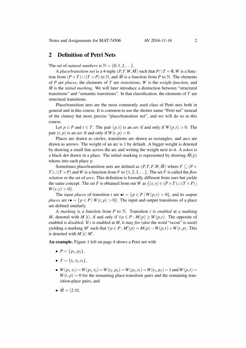
An example. Figure 1 left on page 4 shows a Petri net with

• P = {p1, p2},

• T = {t1, t2, t3},

• W (p1, t1)=W (p1, t2)=W (t2, p2)=W (p2, t3)=W (t3, p1)= 1 and W (p, t)=W (t, p) = 0 for the remaining place-transition pairs and the remaining tran-

sition-place pairs, and

• M = (2,0).


We have F = {(p1, t1),(p1, t2),(t2, p2),(p2, t3),(t3, p1)}. Furthermore, •p1 = {t3}and p1•= {t1, t2}. Also, M [t1〉 and M [t1〉 (1,0). ✷

5. Give a talk on capacities of places and the place / complement place con-

struction.

6. Give a talk on inhibitor arcs of Petri nets.

7. Give a talk on Coloured Petri Nets. Please concentrate on the intuitive idea

instead of the formal definition.

3 Reachability Graphs

The notation M [t1t2 · · · tn〉 M′ means that there are markings M0, M1, . . . , Mn such

that M = M0, Mn = M′, and for each 1 ≤ i ≤ n we have Mi−1 [ti〉 Mi.

A marking M′ is reachable from M if and only if there is a finite sequence σ

of transitions such that M [σ〉 M′. The set of markings that are reachable from M

is R(M) = {M′ | ∃σ ∈ T ∗ : M [σ〉 M′}. (Many authors use the notation [M〉 instead

of R(M).) A marking is reachable if and only if it is reachable from the initial

marking. The set of reachable markings of a Petri net is thus R(M). That is, it is

the set of those markings that can be obtained by starting at the initial marking and

firing any finite sequence of transitions. The opposite of reachable is unreachable.

Also the sequence of zero transitions is a finite sequence of transitions. Any

sequence of zero elements is called the empty sequence and denoted with ε. So

trivially M [ε〉 M holds for each marking M. This says that from any marking,

it is possible to fire nothing, and the result is the same marking. Furthermore,

M ∈ R(M) holds for every marking M.

The reachability graph (also called “occurrence graph”) of a Petri net is the

triple (R(M),∆,M), where ∆ = {(M, t,M′) | M ∈ R(M)∧M [t〉 M′}. The elements

of ∆ are called semantic transitions. Often the word “semantic” is dropped, causing

some risk of confusion with Petri net transitions.

That is, the reachability graph is a directed graph whose vertices are the reach-

able markings and edges are the semantic transitions between the reachable mark-

ings. The initial marking is distinguished.

Reachable markings are usually drawn as circles, ovals, or boxes with rounded

corners. Semantic transitions are drawn as arrows. The initial marking is distin-

guished with an arrow that starts outside all markings and ends at it. A marking M

can be represented as the vector (M(p1), M(p2), . . . , M(p|P|)). However, it often

consumes a lot of space, so it is common to use some denser representation. For

instance, if there always is precisely one token in some subset of places, then the

places may be given numbers, and the number of the marked place is shown in the

dense representation of the marking.

Reachability graphs are an example of state spaces. A state is a description of

the contents of all information-storing elements of a system. The state of a Petri


p1

p2

t1

t2 t3

t1 t1

t1t2 t3 t2 t3

t2 t3

2,0

1,1

0,2

1,0

0,1

0,0

Figure 1: An example Petri net and its reachability graph.

net is the marking. The phrase “state space” is often used informally to mean either

the set of the reachable states of a system or the directed graph that consists of the

reachable states and the semantic transitions between them.

An example. Figure 1 shows an example of a Petri net and its reachability graph.

In the example,

• R(M) = {(0,0),(0,1),(0,2),(1,0),(1,1),(2,0)},

• ∆ = {((2,0), t1,(1,0)),((1,0), t1 ,(0,0)),((2,0), t2 ,(1,1)), . . .}, and

• M = (2,0).

We have (2,0) [t2t1t3〉 (1,0). The marking (0,2) is reachable, but not reachable

from (0,1). The marking (1,2) is unreachable. ✷

8. Draw the reachability graph of this Petri net.

2 3

a b c

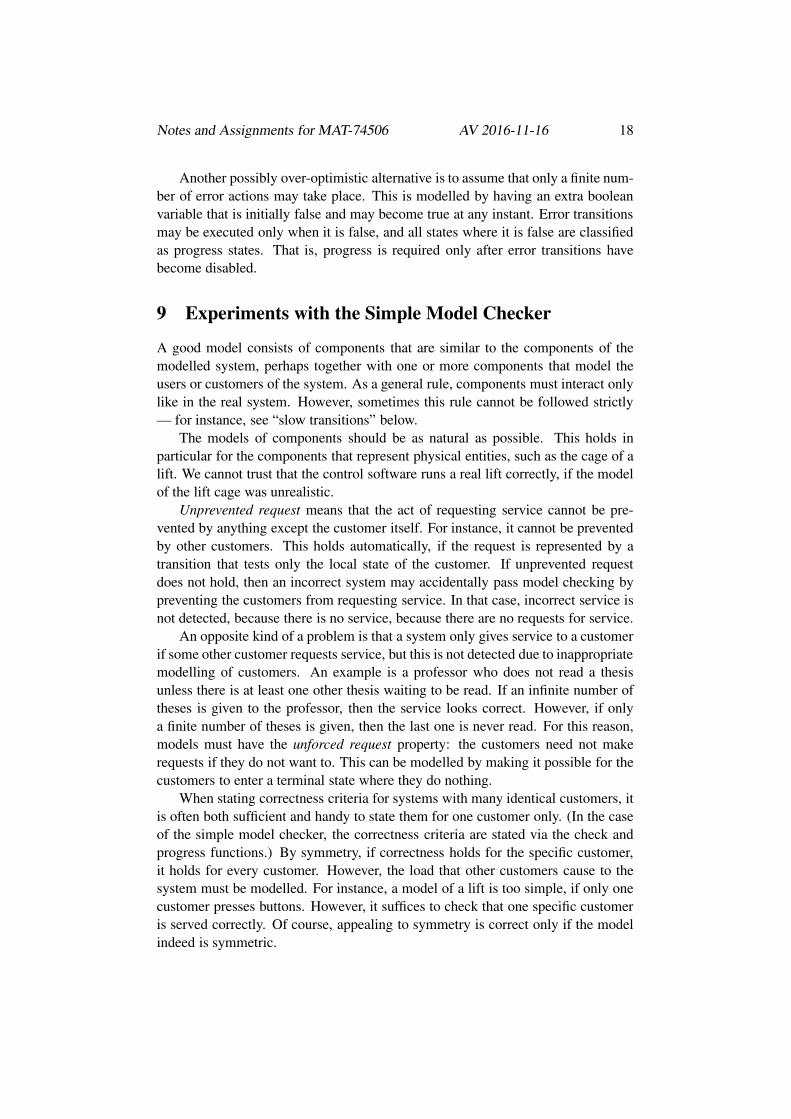
9. The Dining Philosophers’ system consists of n philosophers and n chop

sticks around a round table. Between each philosopher and the next philoso-

pher there is one chop stick. The life of each philosopher is like the follow-

ing:

1: take the chop stick from the left (wait if it is not there)

2: take the chop stick from the right (wait if it is not there)

3: return the chop stick to the left

4: return the chop stick to the right; goto 1

Local state 1 is also known as “thinking”, 2 as “has left”, 3 as “eating”, and 4

as “has right stick”. Philosopher i and the adjacent chop sticks are shown in

Figure 2 as a Petri net. Draw the reachability graph of the one philosophers’

system and of the two philosophers’ system.

10. Draw the reachability graph of the three philosophers’ system.


1itli

2i tri 3irli

4irri

csi

cs(imodn)+1

Figure 2: One dining philosopher as a Petri net.

11. Which of the following hold for all reachable markings M1, M2, and M3?

Justify your answers.

(a) If M2 ∈ R(M1), then M1 ∈ R(M2).

(b) If M2 ∈ R(M1) and M3 ∈ R(M2), then M3 ∈ R(M1).

(c) Either M2 ∈ R(M1) or M1 ∈ R(M2) or both.

(d) If M ∈ R(M1), then M2 ∈ R(M1).

4 Boundedness and Liveness

A place p of a Petri net is k-bounded if and only if for every reachable marking

M we have M(p) ≤ k. A Petri net is k-bounded if and only if its every place is

k-bounded. For instance, the Petri net in Figure 1 is 2-bounded. If a place is k-

bounded, then it also is (k+ 1)-bounded, (k+ 2)-bounded, and so on. A place is

bounded if and only if it is k-bounded for some k ∈ N. A Petri net is bounded if

and only if it is k-bounded for some k ∈N. The opposite of bounded is unbounded.

The simplest example of an unbounded Petri net is the following: . Its

reachability graph is t t t0 1 2 · · · .

Assume that P is finite. The Petri net is bounded if and only if its set of reach-

able markings is finite.

A transition t is dead at a marking M if and only if it is disabled at every element

of R(M). A dead marking is a marking where every transition is dead. Often the

word deadlock is used to mean a state where nothing can happen. With that usage,

a deadlock of a Petri net is the same as a dead marking. However, some authors

distinguish between deadlocks and successful termination. For them, a deadlock

of a Petri net is a marking where every transition is dead although that was not the

purpose.

12. For each of the following properties, draw a Petri net with at least two places

that has the property.

(a) Its all markings are reachable.


(b) It is 3-bounded and all markings that do not violate 3-boundedness are

reachable.

(c) It has precisely three reachable dead markings.

13. Draw a two-bounded Petri net with three places such that its initial marking

is reachable from every reachable marking and it has as many reachable

markings as possible. Justify your answer.

14. Let us say that a Petri net is bounded′ if and only if each of its places is

bounded.

(a) Assume that P is finite. Is bounded′ the same notion as bounded?

(b) Do not assume that P is finite. Is bounded′ the same notion as bounded?

15. (a) Give an example of a Petri net that is bounded and has an infinite num-

ber of reachable markings.

(b) Is there any finite Petri net that is unbounded and only has a finite

number of reachable markings?

16. Four types of liveness are often defined for Petri nets. Give a talk on them.

In the talk, for each 1 ≤ i ≤ 3, give an example of a Petri net that is live-i but

not live-(i+1).

ASSET exercises

17. (This problem is easy. You can make it even easier by fixing n = 2, that is,

only doing (a).)

Model a system consisting of a shared variable and n users, User 0, User 1,

. . . , User (n−1). Each user first takes a local copy of the value of the shared

variable. That is, User i assigns local[i] := shared. Then the user adds 2i to

its local copy, that is, assigns local[i] := local[i]+2i. Finally the user copies

its local value to the shared variable, that is, assigns shared := local[i]. Then

the user terminates. The users run in parallel.

Model the local state of each user with an array element that can get the

value 0, 1, 2, or 3. You can make ASSET print all end results by making

check deadlock call print state and return 0. When i is a small non-

negative integer, 2i can be computed as (1<<i).

(a) Demonstrate with ASSET that if n = 2, then, in the end, shared may

have three different values.

(b) How many different values shared may have in the end, if n = 1, n = 3,

or n = 4?


#define chk_deadlock

const char * check_deadlock(){ return "Illegal deadlock"; }

bool fire_transition( unsigned tr ){

if( tr < 2 ){

if( cli[ tr ] == 0 ){ req[ tr ] = 1; cli[ tr ] = 1; return true; }

if( cli[ tr ] == 1 && gra[ tr ] ){ cli[ tr ] = 2; return true; }

if( cli[ tr ] == 2 ){ req[ tr ] = 0; cli[ tr ] = 0; return true; }

}else{

tr -= 2;

if( server == 0 && req[ tr ] ){ server = 1+tr; return true; }

if( server == 1+tr ){ gra[ tr ] = 1; server = 3+tr; return true; }

if( server == 3+tr && !req[ tr ] ){ server = 5+tr; return true; }

if( server == 5+tr ){ gra[ tr ] = 0; server = 0; return true; }

}

return false;

}

Figure 3: A part of a faulty two-step handshake.

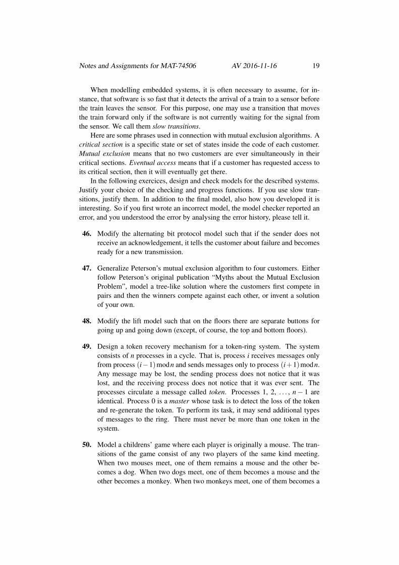
18. (Easy) Figure 3 shows a part of a model of a faulty mutual exclusion system

that consists of a server and two clients. Between Client i (i ∈ {0,1}) and the

server there are two variables, req[i] and gra[i]. Client i requests for access

to the critical section by assigning req[i] := 1. The server grants access by

assigning gra[i] := 1. When Client i leaves the critical section, it assigns

req[i] := 0 and goes back to its initial state. The server reacts to this by

assigning gra[i] := 0. Because the system models low-level hardware, each

transition can do altogether at most one operation (testing, reading, writing)

on the shared variables. For instance, the same transition cannot both detect

that req[0] = 1 and assign gra[0] := 1.

Complete the model. Then detect with ASSET that the model does not guar-

antee mutual exclusion. Finally, fix the model and verify with ASSET that

now it does guarantee mutual exclusion. A transition may access at most one

shared variable and do at most one operation (test, read, write) to it.

19. A camel can walk one camel-distance in a day. A desert is 12 camel-dis-

tances wide. The camel and its rider consume one unit of resources (water,

food, etc.) each day. The camel can carry 6 units in addition to the rider.

For instance, the camel can take 6 units of resources, walk 2 days into the

desert consuming 2 units of resources, leave 2 units there, and walk back

consuming the last 2 of the 6 units that it originally took. Later on the camel

can use the resources that had been left in the desert. How many units of

resources are needed to cross the desert?

20. A ring consists of n squares, where n ≥ 10. Find the smallest n such that the

following is possible. A grasshopper is on one of the squares. Nine squares


& ¬

& ¬

Figure 4: An arbiter circuit.

to the right of the grasshopper there is a trap square where the grasshopper

must never go. (If n = 10, then the trap is next to the left from the grasshop-

per’s original position.) The grasshopper also must never go back to a square

where it has already been. On step 1, the grasshopper jumps one square to

the left or to the right. On step 2, it jumps two squares to the left or to the

right, and so on. On the last step, it jumps n− 2 squares to the left or right.

Then it has visited all the squares except the trap.

21. There is a peg on each but one square of a 5 times 5 grid. The empty square

is in the middle of the leftmost row. A move consists of a peg moving two

squares left, right, up, or down such that it jumps over a peg and enters in an

empty square. The peg that is jumped over is removed. Find a sequence of

moves that leaves only one peg on the grid.

22. Alice and Bob are runners and digital electronic designers. They want to

know which one is the faster runner, but they are so equally fast that they

never see any difference. Therefore, they build the circuit shown in Figure 4.

When Alice or Bob gets to the goal, she or he presses her or his button,

causing the output of the button to change from 0 to 1. The output of the

button never goes back to 0. The circuit switches one of two LED lamps

on, telling who pressed first. The lamps are denoted with ⊗. The output of

a gate denoted with & is the logical and of its inputs. The output of a gate

denoted with ¬ is the logical negation of its input. Each transition sets the

output of one gate whose output is currently wrong or models the pressing

of a button. Show with ASSET that the system may fail to stop but cannot

lose the ability to stop.

23. There are n people who want to select a leader from among them. Everybody

must have the same probability of becoming the leader. They have coins

that, when tossed, yield 0 (tail) or 1 (head) with the same probability. First

the people considered organizing a cup, but soon they realized that to get

equal probabilities, n must be a power of 2. Then someone invented a ring

algorithm that gives equal probabilities because the system is symmetric.


Client i

0: ri := T [] goto 4

1: wait gi

2: ri := F

3: wait ¬gi; goto 0

4:

Server i

0: get token from previous server

1: if ¬ri then goto 5

2: gi := T

3: wait ¬ri

4: gi := F; goto 1

5: give token to next server; goto 0

Figure 5: The client and server of a token ring.

The people form a ring. Everyone can communicate with the previous and

the next person in the ring, but not with the others. Everyone has a suggestion

for the leader. Initially everyone suggests her- or himself. At any time, if two

adjacent people have different suggestions, they may agree on a common

suggestion by tossing a coin. The loser copies the suggestion of the winner

to itself. A transition may only access the variables of two adjacent persons,

but it may test, read from, and write to the variables of those two persons as

much as you want.

(a) For three different values of n that must be at least 3 (other than this,

you may choose them freely), show with ASSET that the system may

fail to stop but cannot lose the ability to stop.

(b) Show mathematically that when n is not a power of 2, there is no al-

gorithm that is guaranteed to stop and where everybody has the same

probability of becoming the leader.

24. (Not easy) The people tried the algorithm developed in the previous exercise

and realized that they cannot find out when it has stopped. Modify the algo-

rithm such that in the end, everyone agrees on the leader and everyone knows

that the leader has been found. A transition may only access the variables of

two adjacent persons, but it may test, read from, and write to the variables of

those two persons as much as you want.

25. A token-ring mutual exclusion system consists of n clients and n servers,

shown in Figure 5. Each client and server communicate via two Boolean

variables ri and gi. “xxx [] yyy” means that the process executes either xxx or

yyy.

(a) Write an ASSET model of the system with a check state function that

verifies mutual exclusion, check deadlock that verifies that each client has

terminated properly, and is may progress that verifies that client 0 cannot

be blocked into the state where it has requested for access to the critical

section but is not yet in the critical section.

(b) Demonstrate that if there are initially no tokens in the ring, the system works

incorrectly. Explain the error.


(c) Demonstrate that if there is initially one token in the ring, the system works

correctly.

(d) Demonstrate that if there are initially two tokens in the ring, the system

works incorrectly. Explain the error.

(e) Demonstrate that if there is initially one token in the ring and must-progress

is required instead of may-progress, the system works incorrectly. Explain

the error.

26. Modify the system of item (e) of the previous exercise so that although must-

progress is required, it works correctly.

27. Replace line 1 of the servers in the previous exercise by “wait ri”.

(a) Demonstrate that the system works incorrectly. Explain the error.

(b) Demonstrate that if “[] goto 4” is removed from the clients, then ASSET

detects no errors. Explain why the error is not detected.

5 Strong Components

A strong component of a directed graph is a maximal nonempty set of vertices such

that for any two vertices in the set, there is a path from the first to the second and a

path from the second to the first. Also a longer name maximal strongly connected

component is used. Each vertex belongs to precisely one strong component.

In the case of the reachability graph of a Petri net, if M ∈ R(M), then the strong

component that M belongs to is {M′ | M′ ∈ R(M)∧M ∈ R(M′)}.

Concurrent systems are often expected to be able to run indefinitely long: after

giving money to some customer, a cash dispenser should be able to give money

to the next customer; and after carrying one customer to some floor, a lift should

be ready to carry the next customer. Therefore, at least as seen from the outside,

the system must always be able to come back where it was and do the same thing

again.

On the other hand, it follows immediately from the definition of strong com-

ponents that if a system leaves a strong component, then it cannot come back.

Therefore, the existence of more than one strong component may be a sign of an

error. However, there are also legal reasons for extra strong components. For in-

stance, if the system can be switched off, then it correctly has a chain of strong

components leading to a dead state. Strong component analysis has been used as

a method of finding errors of certain kinds. However, nowadays there are better

methods that do not yield false positives.

A strong component C is terminal if and only if the system cannot leave it.

That is, if M ∈C and M [t〉M′, then also M′ ∈C. The opposite is nonterminal. A

strong component C is acyclic if and only if every edge that starts at it leaves it.


1 Found := {M}; Work := {M}2 while Work 6= /0 do

3 choose some M ∈ Work

4 if M has no transitions left then Work := Work \{M}; goto 2

5 let t be the next transition at M

6 if ¬M [t〉 then goto 2

7 let M′ be the marking such that M [t〉M′

8 if M′ /∈ Found then Found := Found∪{M′}; Work := Work∪{M′}9 ∆ := ∆∪{(M, t,M′)}

Figure 6: The basic reachability graph construction algorithm.

The opposite is cyclic. That is, C is cyclic if and only if it contains two markings

M and M′ such that there is t such that M [t〉M′. Here M and M′ are not necessarily

different.

28. Draw a directed graph such that its every vertex is reachable from the vertex

that you draw first, and it has precisely four strong components. One of the

components is terminal cyclic, one is terminal acyclic, one is nonterminal

cyclic, and one is nonterminal acyclic.

29. Give a talk on efficient algorithms for finding strong components.

6 Constructing Reachability Graphs

Figure 6 shows the principle of the construction of reachability graphs. There are

two main data structures: Found keeps track of the markings that have been found,

and Work keeps track of work that still has to be done. Each marking in Work keeps

track of which transitions have been tried at the marking.

Initially only M has been found. Because it has not yet been investigated, it

is put to Work. The main loop starts by picking some marking M from Work and

checking whether all transitions have been investigated at it. If yes, then M has

been fully investigated and is removed from Work. In the opposite case, the first

transition that has not yet been investigated at M is chosen. If it is enabled, it is

fired. If the resulting marking has not yet been found, it is added to Found and

Work. On line 9, the edge is added to the set of edges. The set ∆ and line 9 can be

dropped from the algorithm if ∆ is not needed.

We see that always when a new marking is found, it is put to both Found and

Work. It stays permanently in Found. While it is in Work, each transition is tried at

it in an unspecified order. When every transition has been tried at it, it is removed

from Work.

Often the order in which markings are chosen on line 3 is specified. In breadth-

first search, always the marking that has been the longest time in Work is chosen.

That is, Work operates as a first-in first-out queue. Such an implementation may


try the transitions in a for-loop instead of going from lines 6 and 9 back to line 2

to pick the next transition.

In depth-first search, always the marking that has been the shortest time in

Work is chosen. That is, Work is used as a stack. The execution must go back to

line 2 after each firing of a transition. Depth-first search has a simple recursive im-

plementation where Work is not implemented explicitly. Unfortunately, recursion

reduces speed and increases memory consumption. Construction of reachability

graphs is often a bottleneck, so its implementation should be as efficient as possi-

ble.

Always Work ⊆ Found. Usually Found is implemented as a hash table. The

implementations of Work vary a lot. Although in the abstract representation both

Found and Work contain markings, memory can be saved by making Work contain

pointers to markings instead of markings, so that the markings are not stored twice.

Tried transitions can be kept track of by adding an extra field to the marking record

that stores the number of (or a pointer to) the transition that was tried last.

In addition to the state of the system as a whole, it is often handy to talk about

the state of an individual component. To distinguish between these two uses, the

state of the system as a whole is called the global state and the state of an individual

component is a local state.

30. Write a breadth-first reachability graph construction algorithm and a recur-

sive depth-first reachability graph construction algorithm. Only show the

same level of detail as Figure 6 shows.

31. Give a talk on Sections 1 to 6 of “What the Small Rubik’s Cube . . . ” in the

reading material.

32. Give a talk on Sections 7 to 11 of “What the Small Rubik’s Cube . . . ” in the

reading material.

33. Draw the reachability graph of Peterson’s mutual exclusion algorithm, as

found in Valmari & Setala: Visual Verification of Safety and Liveness.

34. Consider the Dining Philosophers’ system.

(a) Design a representation of the global state. Try to use as few bits as

possible. How many bits (as a function of n) are used?

(b) Assume that the local states of the philosophers and chop sticks are

stored in int Ph[n] and int Cs[n] , respectively. Write program

code for packing and unpacking the state.

(c) Derive an upper bound to the number of reachable states as a function

of n.

35. A simplified version of the alternating bit protocol over unreliable channels

consists of a sender S, a receiver R, and two channels D and A. The purpose


of the system is to reliably deliver messages from C1 to C2. For simplic-

ity, we assume that there are two different messages: “Y” and “N”. The

notation “code1 [] code2” denotes that either code1 or code2 is executed. If

both code1 and code2 are enabled, then the choice between them is arbitrary.

Each send- and its corresponding receive-statement are executed simultane-

ously. So, for instance, “send 〈m,b〉 to D” is disabled as long as D contains

a message.

The components operate as follows:

S (b is a local variable with initial value 0)

1: receive m from C1;

2: send 〈m,b〉 to D; goto 2

[] receive a from A; if a 6= b then goto 2 else b := 1−b; goto 1

R (a is a local variable with initial value 0)

1: receive 〈m,b〉 from D

2: if b = a then send m to C2; a := 1−a endif

3: send b to A; goto 1

D

1: receive 〈m,b〉 from S;

2: send 〈m,b〉 to R; goto 1

[] goto 1

A

1: receive a from R;

2: send a to S; goto 1

[] goto 1

(a) How many local states do A and its a have together? Please notice that

the value of a need not be remembered while A is in its local state 1.

Leave out unnecessary data also in (b), (c), and (d).

(b) How many local states do D, m, and b have together?

(c) How many local states do R and its variables have together?

(d) How many local states do S and its variables have together?

(e) Write program code for packing and unpacking the state.

(f) Derive an upper bound to the number of reachable states.

36. Draw the reachability graph of the simplified alternating bit protocol of the

previous problem. To make the task easier, use only the message “Y” and

do not draw states that are symmetric to already drawn states with respect to

the b of S and the a of R.

37. Why is the alternating bit necessary also in the messages that go from R to S

via A?

7 Checking Properties from the State Space – Part 1

A state proposition is a yes/no-claim that holds or does not hold on an individual

state. “The lift is at floor 3” and “place p5 contains two tokens” are state propo-


sitions. “The lift will be at floor 3 some time in the future” and “in all reachable

markings, p5 contains at most two tokens” are not state propositions.

There are rich languages for expressing state propositions and complicated al-

gorithms for checking whether or not a given state proposition holds on a given

state. However, from the point of view of model checking they are a separate prob-

lem area that does not interfere much with the hard problems of model checking.

Research on languages, parsing, etc., has provided good tools for expressing state

propositions and checking whether they hold. In model checking, it is typically

just assumed that there is a set of state propositions and a practical way of deciding

whether s |= π, that is, whether state proposition π holds on state s.

A complementary way of encoding “elementary” information for model check-

ing is visible labels of structural transitions. That is, a structural transition (e.g., an

atomic statement of the program code or a Petri net transition) is given a name that

reflects its role in the service provided by the system. “The lift opens its doors” or

“20 euros are given to the customer” are examples. More than one transition may

have the same label.

Typically many transitions lack visible labels, because what they do is not im-

mediately visible to the user. An example is the transition with which the cash

dispenser sends the “20 euro withdraw request” message to the bank. Such transi-

tions are invisible. It is handy to reserve a special label for denoting the absence of

a visible label. Often τ is used for this purpose. So when we say that the label of

a transition is τ or that the transition is invisible, we mean that the transition does

not have a label that tells about its role.

Often it is easy to replace state propositions by visible labels. For instance, “the

lift is at floor 3” can be replaced by “the lift arrives floor 3” and “the lift leaves floor

3”. Replacing visible labels by state propositions may require adding one or more

variables to which visible transitions store information. For instance, a variable

may remember the most recent withdraw request that the user of a cash dispenser

has made.

Properties that refer to the history of the state can often be encoded as state

propositions by adding suitable code to the model, analogously to adding test code

or testing equipment to a real system. Consider the cash dispenser again. Assume

that when the customer makes a withdraw request, the amount is stored in an extra

variable. Later, when the money is given, the given amount can be compared to

the requested amount and a state proposition can be set to True if they are not the

same.

The idea of collecting information from the history and detecting that it obeys

some specific pattern is the idea behind classical finite automata. Indeed, finite

automata can be used in model checking by synchronising the automaton with (a

subset of) visible labels. However, it is often easier to implement the collection

and analysis of the history information in ordinary program code, using the same

language as for modelling the system under analysis.

Instead of detecting the error from some state proposition or some formula

on state propositions becoming True, the error may be detected from some error


detection transition becoming enabled. An error detection transition is a structural

transition that has been added to the system for this purpose. A natural candidate

is the transition that sees that the requested and given amounts of money are not

the same.

From now on it is assumed that some mechanism for checking individual states

exists. It is not important whether it is based on individual state propositions,

formulae on states, or error detection transitions.

In the state space construction algorithm, the best place to check a state against

errors is immediately after it has been detected that it is not in Found (line 8 in

Figure 6). In general, it is better to detect errors as early as possible, because

otherwise it may happen that the erroneous state has been constructed after the first

ten minutes but is detected only after ten hours. On the other hand, testing that the

state is not in Found is fast. By doing it first, the algorithm avoids checking the

same state against errors each time it is found anew.

If the tool reveals, for instance, that a banking system can take money from a

wrong account, the user of the tool typically wants to analyse how that can happen.

For that, a counterexample is often helpful. It is a path from the initial state to the

error, listing the details of the states along the path, the full names of the structural

transitions whose occurrences caused the edges of the path, or both. Breadth-first

search yields as short counterexamples as possible. Depth-first search tends to

yield long counterexamples that contain also many events that have nothing to do

with the error.

38. Add code to the alternating bit protocol that checks that the message that is

received is the same as the message that was sent. It communicates with the

protocol via the statements “send m to S” and “receive m from R”. Assume

that the language contains the statement error “text” with which errors can

be signalled.

39. A building has n floors. At each floor there are buttons △ (up) and ▽ (down)

with the two obvious exceptions. Inside the lift cage there is a button for each

floor. For each floor, a signal is available that tells that the lift stopped at that

floor. Ignore the opening and closing of the doors. Write code that checks

that the lift stops at the right floors.

40. Consider the n dining philosophers’ system as described in an earlier exer-

cise. How long is the shortest path from the initial state to the deadlock?

How long is the path constructed by depth-first search, assuming that the al-

gorithm tries first the transitions of philosopher 1, then of philosopher 2, and

so on? If you cannot solve this problem for n in general, solve it for n = 2

and n = 3.

41. Download the simple model checker and the alternating bit protocol model

from the course web page. By modifying the model, running the checker,

and analysing the result, answer the following questions.


(a) What goes wrong, if the data channel does not have the alternating

bit? (Hint: comment out the checking that the data message carries the

right bit value, and the transition that receives the data message with

the wrong bit value.)

(b) What goes wrong, if the acknowledgement channel does not have the

alternating bit?

(c) Can something go wrong, if the channels cannot lose messages?

42. Make changes to the alternating bit protocol model that do not invalidate it

for model checking but do reduce the size of its state space. How small can

you make it?

43. Modify the alternating bit protocol model by merging the states on both sides

of the sender timeout transition. Does it work correctly? Does it work cor-

rectly, if the channels cannot lose messages?

44. Write a new model for the alternating bit protocol that only uses a small

number of transition numbers. For instance, all transitions of the receiver

may have the same number, because more than one of them are never simul-

taneously enabled.

45. Model a lift for the simple model checker. The building must have at least

four floors. The model must contain at least one component for the lift cage

and at least one component for the software that receives signals from the

buttons and floor sensors and sends commands to the motor that moves the

lift cage up and down.

8 Checking Properties from the State Space – Part 2

The machinery of the previous section suffices for verifying so-called safety prop-

erties, that is, detecting if something happens that should not happen. It does not

suffice for verifying so-called liveness or progress properties, that is, detecting if

something fails to happen that should happen. For instance, that the lift does not

stop at a wrong floor is a safety property, because if the lift stops at a wrong floor

then one can say that now the property is violated. That the lift eventually arrives

is a liveness property, because even if it has not yet arrived, it is possible that it will

arrive in the next five seconds, five minutes, or five centuries.

It is typical of liveness properties that in real life it is never possible to say that

the property has been violated. However, it is often possible to detect violations

of liveness properties from state spaces, by detecting infinite executions where the

awaited thing (like the arrival of the lift) does not happen. So liveness proper-

ties can never be tested, although they can often be model-checked. In real life,

violations of liveness properties manifest themselves by the system not respond-

ing within a “reasonable” time. What we really want is not liveness but “short


enough” response times. However, liveness is often a reasonable abstraction for

“quickly enough”. This is similar to the fact that often in programming, integers

are discussed instead of 32-bit integers.

At this stage it is appropriate to give a warning: in Petri net literature, the

concept of “safe Petri net” has been defined, but it is not the same as the safety that

has been discussed above.

We saw in the previous section that it is easy to make state space construction

tools detect violations of safety properties. Another class of easily detectable error

situations consists of illegal deadlocks. It suffices that some specific state propo-

sition or formula tells whether termination is allowed. Each time when the tool

detects that a state does not have enabled transitions, it checks whether the formula

yields True. If it does not, the tool reports an illegal deadlock.

Literature disagrees on whether freedom from illegal deadlocks is a safety

property. The opinion of the present author is that it is better to consider it as a

class of its own, but if it must be classified as safety or liveness, it is liveness.

Non-progress is a subclass of relatively easily detectable liveness errors. The

structural transitions of the system are divided to two classes: ordinary transitions

and progress transitions. For instance, the visible transitions may be declared as

progress transitions while the invisible transitions are ordinary. The question is

then “does the state space contain a non-progress cycle, that is, a cycle such that all

edges in it are caused by occurrences of ordinary transitions?” The counterexample

consists of a sequence that leads from the initial state to a non-progress cycle,

followed by the cycle. The same idea can be implemented using states instead

of transitions. In the simple model checker, such states are called “must-type”

progress states.

Liveness properties often depend on complicated assumptions. For instance, if

a channel can lose messages without limit, then it is impossible to guarantee that

a protocol always eventually delivers the message that it was given for delivery.

Therefore, it is often assumed that the channel can only lose a finite number of

messages in a row. This is an example of a strong fairness assumption: if some

transition is enabled infinitely often (the transition that represents correct channel

operation), then it is executed infinitely often. However, with a more complicated

protocol it may be that two successive messages (such as a connection request and

a data message) must get through the channel for successful delivery. Then a more

complicated strong fairness assumption is needed.

For this reason, sometimes a simple but somewhat over-optimistic global fair-

ness assumption is made: if a choice situation is encountered infinitely often, then

each of the choices is taken infinitely often. By “global” it is meant that the model

checker makes it automatically, so the user need not model it. In terms of (finite)

state spaces this means that unreachability of the desired action is considered an

error, but the existence of a cycle that does not contain the desired action is not

considered an error as such. In the simple model checker, this is represented via

“may-type” progress states. The checker declares an error when a state is reached

from which no may-type progress state can be reached.


Another possibly over-optimistic alternative is to assume that only a finite num-

ber of error actions may take place. This is modelled by having an extra boolean

variable that is initially false and may become true at any instant. Error transitions

may be executed only when it is false, and all states where it is false are classified

as progress states. That is, progress is required only after error transitions have

become disabled.

9 Experiments with the Simple Model Checker

A good model consists of components that are similar to the components of the

modelled system, perhaps together with one or more components that model the

users or customers of the system. As a general rule, components must interact only

like in the real system. However, sometimes this rule cannot be followed strictly

— for instance, see “slow transitions” below.

The models of components should be as natural as possible. This holds in

particular for the components that represent physical entities, such as the cage of a

lift. We cannot trust that the control software runs a real lift correctly, if the model

of the lift cage was unrealistic.

Unprevented request means that the act of requesting service cannot be pre-

vented by anything except the customer itself. For instance, it cannot be prevented

by other customers. This holds automatically, if the request is represented by a

transition that tests only the local state of the customer. If unprevented request

does not hold, then an incorrect system may accidentally pass model checking by

preventing the customers from requesting service. In that case, incorrect service is

not detected, because there is no service, because there are no requests for service.

An opposite kind of a problem is that a system only gives service to a customer

if some other customer requests service, but this is not detected due to inappropriate

modelling of customers. An example is a professor who does not read a thesis

unless there is at least one other thesis waiting to be read. If an infinite number of

theses is given to the professor, then the service looks correct. However, if only

a finite number of theses is given, then the last one is never read. For this reason,

models must have the unforced request property: the customers need not make

requests if they do not want to. This can be modelled by making it possible for the

customers to enter a terminal state where they do nothing.

When stating correctness criteria for systems with many identical customers, it

is often both sufficient and handy to state them for one customer only. (In the case

of the simple model checker, the correctness criteria are stated via the check and

progress functions.) By symmetry, if correctness holds for the specific customer,

it holds for every customer. However, the load that other customers cause to the

system must be modelled. For instance, a model of a lift is too simple, if only one

customer presses buttons. However, it suffices to check that one specific customer

is served correctly. Of course, appealing to symmetry is correct only if the model

indeed is symmetric.


When modelling embedded systems, it is often necessary to assume, for in-

stance, that software is so fast that it detects the arrival of a train to a sensor before

the train leaves the sensor. For this purpose, one may use a transition that moves

the train forward only if the software is not currently waiting for the signal from

the sensor. We call them slow transitions.

Here are some phrases used in connection with mutual exclusion algorithms. A

critical section is a specific state or set of states inside the code of each customer.

Mutual exclusion means that no two customers are ever simultaneously in their

critical sections. Eventual access means that if a customer has requested access to

its critical section, then it will eventually get there.

In the following exercices, design and check models for the described systems.

Justify your choice of the checking and progress functions. If you use slow tran-

sitions, justify them. In addition to the final model, also how you developed it is

interesting. So if you first wrote an incorrect model, the model checker reported an

error, and you understood the error by analysing the error history, please tell it.

46. Modify the alternating bit protocol model such that if the sender does not

receive an acknowledgement, it tells the customer about failure and becomes

ready for a new transmission.

47. Generalize Peterson’s mutual exclusion algorithm to four customers. Either

follow Peterson’s original publication “Myths about the Mutual Exclusion

Problem”, model a tree-like solution where the customers first compete in

pairs and then the winners compete against each other, or invent a solution

of your own.

48. Modify the lift model such that on the floors there are separate buttons for

going up and going down (except, of course, the top and bottom floors).

49. Design a token recovery mechanism for a token-ring system. The system

consists of n processes in a cycle. That is, process i receives messages only

from process (i−1)modn and sends messages only to process (i+1)modn.

Any message may be lost, the sending process does not notice that it was

lost, and the receiving process does not notice that it was ever sent. The

processes circulate a message called token. Processes 1, 2, . . . , n− 1 are

identical. Process 0 is a master whose task is to detect the loss of the token

and re-generate the token. To perform its task, it may send additional types

of messages to the ring. There must never be more than one token in the

system.

50. Model a childrens’ game where each player is originally a mouse. The tran-

sitions of the game consist of any two players of the same kind meeting.

When two mouses meet, one of them remains a mouse and the other be-

comes a dog. When two dogs meet, one of them becomes a mouse and the

other becomes a monkey. When two monkeys meet, one of them becomes a


mouse and the other becomes a human. Humans do not participate meetings.

Based on model checking results with different numbers of players, state a

hypothesis on the possible end situations of the game. Can you confirm the

hypothesis by reasoning?

51. Model an airline reservation system that consists of an airline company and

at least two travel agencies. The travel agencies may reserve flights from the

airline company one at a time. They may also cancel reservations. Between

any two reservations and/or cancellations, the other travel agencies may per-

form reservations and/or cancellations. A customer of a travel agency wants

a sequence of flights such that if it is not possible to get all flights in the se-

quence, then the customer takes no flights at all. This implies that the travel

agency must try to reserve the flights of the sequence one at a time, and if it

cannot get them all, then it must cancel those that it did get.

To the extent that you can, ensure that as many customers as possible get

their flights. To obtain that goal, it may help to add a third value to the

airline database: “confirmed”, meaning that the travel agency succeeded in

getting all the flights that the customer wanted, and thus will not cancel the

flight.

10 Linear Temporal Logic

A linear temporal logic (abbreviated LTL) formula is of any of the following forms,

where π is a state proposition (see Section 7), and ϕ and ψ are linear temporal logic

formulae:

π (ϕ) ϕ∧ψ ϕ∨ψ ¬ϕ ϕ → ψ ϕ ↔ ψ ©ϕ ✷ϕ ✸ϕ ϕ U ψ

An LTL formula holds or does not hold on an infinite sequence of states. It may

help to think about a sequence of days, starting today. With that interpretation,

• ©ϕ is read as “next ϕ”. It holds today if and only if ϕ holds tomorrow.

• ✷ϕ is read as “always ϕ”. It holds today if and only if ϕ holds today, tomor-

row, the day after tomorrow, and so on.

• ✸ϕ is read as “eventually ϕ”. It holds today if and only if ϕ holds today or

some day in the future.

• ϕ U ψ is read as “ϕ until ψ”. It holds today if and only if ψ holds today

or some day in the future, and every day between today and that day, today

included but that day excluded, ϕ holds every day.

The parentheses ( and ) have the same purpose as in many places in mathematics:

they specify how a formula is constructed from subformulae. The operators ∧, ∨,

¬, →, and ↔ are the familiar logical operators “and”, “or”, “not”, “implies”, and


“is logically equivalent to”. If it is claimed that an LTL formula holds without

mentioning the day, then the intention is that it holds today.

That an LTL formula ϕ holds on an infinite sequence s0s1 · · · of states is written

as s0s1 · · · |= ϕ and formally defined as follows:

• s0s1 · · · |= π holds if and only if s0 |= π holds, that is, π holds on the first state

of the sequence. (Because π is a state proposition, whether or not it holds on

the first state only depends on the first state.)

• s0s1 · · · |= (ϕ) holds if and only if s0s1 · · · |= ϕ holds. (The parentheses have

no semantic effect.)

• s0s1 · · · |= ϕ∧ψ holds if and only if both s0s1 · · · |= ϕ and s0s1 · · · |= ψ hold.

• s0s1 · · · |= ϕ∨ψ holds if and only if either s0s1 · · · |= ϕ, s0s1 · · · |= ψ, or both

hold.

• s0s1 · · · |= ¬ϕ holds if and only if s0s1 · · · |= ϕ does not hold.

• s0s1 · · · |=ϕ→ψ holds if and only if s0s1 · · · |=ϕ does not hold or s0s1 · · · |=ψ

holds.

• s0s1 · · · |= ϕ ↔ ψ holds if and only if either none or both of s0s1 · · · |= ϕ and

s0s1 · · · |= ψ hold.

• s0s1 · · · |=©ϕ holds if and only if s1s2 · · · |= ϕ holds, that is, ϕ holds on the

sequence that is obtained from the original by removing the first state.

• s0s1 · · · |=✷ϕ holds if and only if for every i ≥ 0 we have sisi+1 · · · |= ϕ.

• s0s1 · · · |=✸ϕ holds if and only if for some i ≥ 0 we have sisi+1 · · · |= ϕ.

• s0s1 · · · |= ϕ U ψ holds if and only if there is i such that ψ |= sisi+1 · · ·, and

for 0 ≤ j < i we have ϕ |= s js j+1 · · ·.

An LTL formula holds on a system if and only if it holds on every complete

execution of the system. A complete execution starts at the initial state and ei-

ther ends in a deadlock or never ends. For each complete execution, the formula

is checked against the infinite sequence of states that the states of the execution

constitute. In the case of a deadlocking execution, its last state is repeated for-

ever to get an infinite sequence of states. That is, if the sequence of states of the

execution is s0s1 · · · sn and sn is a deadlock, then the formula is checked against

s0s1 · · · sn−1snsnsn · · ·.If an LTL formula does not hold on a system, then the system has a complete

execution that violates the formula (and vice versa). This execution can be given as

a counterexample. It is analogous to a test run where the system failed. Checking

whether the formula holds on the system is equivalent to checking whether the

system has an execution that satisfies the negation of the formula.

Some operators can be expressed in terms of the others:


ϕ∨ψ ⇔ ¬(¬ϕ∧¬ψ) ✸ϕ ⇔ True U ϕ

ϕ → ψ ⇔ ¬ϕ∨ψ ✷ϕ ⇔ ¬✸¬ϕ

ϕ ↔ ψ ⇔ (ϕ → ψ)∧ (ψ → ϕ)

Intuitively also the following hold:

✸ϕ ⇔ ϕ∨©ϕ∨©©ϕ∨ ·· · and ✷ϕ ⇔ ϕ∧©ϕ∧©©ϕ∧ ·· · .

However, the formulae on the right hand sides are infinite. Therefore, they cannot

be processed by computers.

An LTL formula is stuttering-insensitive if and only if its validity does not

depend on the number of times that a state repeats in a row, as long as the number

is finite. In practice it means that it does not matter whether a banking system made

one, five, or one hundred transitions before giving money. Let r denote “request”

and s denote “service”. The formula

✷(r→✸s)

specifies that every request that is made today or later is eventually served. (The

service must come at the same time as or later than the request. Requests and ser-

vices are not counted. That is, one service suffices to satisfy all earlier requests and

even a simultaneous request.) The formula is stuttering-insensitive. An example of

a stuttering-sensitive formula is ✷(r →©©©s). It says that each request must

be served precisely three states later.

Typically we want specifications be stuttering-insensitive. A formula is cer-

tainly stuttering-insensitive, if it does not contain the operator ©. Therefore, we

typically do not use © in specifications.

However, © is important for explaining algorithms for checking whether a

system satisfies a formula. They often exploit the following fact, or its analogue to

✷ and ✸ (the analogues can be derived from formulae given above and ¬©ϕ ⇔©¬ϕ):

ϕ U ψ ⇔ ψ∨ϕ∧©(ϕ U ψ)

To understand its significance, consider the problem of deciding whether ϕ U ψ

holds on some state of some infinite path through a finite state space. Any infinite

path through a finite state space eventually starts to go around one or more cycles.

To simplify the discussion, we assume that the path consists of a (possibly empty)

initial part and one cycle. Let s0s1 · · · denote the corresponding sequence of states.

Assume that for every si, it is already known whether sisi+1 · · · |= ϕ and sisi+1 · · · |=ψ.

If ψ holds on the current state, then also ϕ U ψ holds on the current state. If

neither ϕ nor ψ holds on the current state, then also ϕ U ψ does not hold on the

current state. Otherwise the result depends on whether ϕ U ψ holds on the next

state of the sequence. So the algorithm goes there. If the algorithm repeatedly goes

to the next state without finding the answer, it eventually goes around the cycle. At

that point it is certain that ψ does not hold in the rest of the infinite path. So ✸ψ

and thus ϕ U ψ do not hold.


52. Which of the following hold? Justify your answers.

(a) ©©ϕ ⇔ ©ϕ (f) ✷(ϕ∨ψ) ⇔ (✷ϕ)∨✷ψ

(b) ✷✷ϕ ⇔ ✷ϕ (g) ✷(ϕ∧ψ) ⇔ (✷ϕ)∧✷ψ

(c) ✸✸ϕ ⇔ ✸ϕ (h) ✸✷✸ϕ ⇔ ✷✸ϕ

(d) ©✷ϕ ⇔ ✷©ϕ (i) ✷✸✷ϕ ⇔ ✸✷ϕ

(e) ©✸ϕ ⇔ ✸©ϕ (j) ¬(ϕ U ψ) ⇔ (✷¬ψ)∨ (¬ψ U¬ϕ)

53. Let ϕ1 and ϕ2 be any two formulae from the following list. Give all implica-

tions of the form ϕ1 ⇒ ϕ2 that hold.

ϕ ©ϕ ✷ϕ ✸ϕ ©✷ϕ ©✸ϕ ✷✸ϕ ✸✷ϕ

54. Using the laws in this document, the laws of propositional logic, and other

laws that you can justify, prove the following:

(a) ¬✷(r→✸s) ⇔ ✸(r∧✷¬s)

(b) ¬((✷✸r)→✷✸s) ⇔ (✷✸r)∧✸✷¬s

55. Is ϕ U (ψ U ζ) equivalent to (ϕ U ψ)U ζ?

56. Let ϕ1(x)⇔ x, ϕ2(x)⇔✷x, ϕ3(x)⇔✸x, ϕ4(x)⇔✷✸x, and ϕ5(x)⇔✸✷x.

Let a be a state proposition. Let 1 ≤ i ≤ j ≤ 5. Which of the formulae of the

form ϕi(a)∧ϕ j(¬a) can hold?

11 Fairness

Catching bad states and bad terminal states is unproblematic both for modellers

and model checking tools. However, they do not check liveness properties beyond

what can be reasoned from terminal states. With only them, it may happen that

if the verification model is so badly wrong that the customers do not issue any

requests in it, then it passes verification. Because there are no requests, there are

no incorrectly served requests.

May-type progress is in a many ways good solution to this problem. It is easy

for the modeller, because so-called fairness assumptions that are the topic of the

rest of this section are not needed. It is easy to implement in verification tools that

do not aim at maximum performance. It works together with stubborn sets that are

a method of reducing the number of states that must be constructed.

However, may-type progress also has negative aspects. The progress guarantee

that it gives is not always strong enough. For instance, when verifying Peterson’s

algorithm, it is important to catch must-type livelocks, because one goal of the al-

gorithm is to guarantee that there are none. If the state space is incompletely con-

structed, like with Holzmann’s bit state hashing, then false alarms may be given.


A counterexample consists of an execution that leads to a state from which no

progress state is reachable. It is not necessarily obvious what information to give

to the modeller, to help her/him find out why progress states are unreachable.

The classical approach with LTL consists of weak fairness and strong fairness.

It is perhaps easiest to understand them as means of ruling out counterexamples

that must not be classified as counterexamples. To discuss this, let us consider a

model consisting of two customers, two travel agencies and one airline company.

Customer 1 negotiates with travel agency 1 and customer 2 with travel agency 2.

During and based on the negotiation, the travel agency reserves flights from the

airline company.

Without any fairness assumptions, must-type verification reports that customer

1 may fail to get the flight, because the system may run around in a cycle where

customer 2 negotiates, travel agency 2 makes a reservation, customer 2 leaves, and

a new customer 2 comes and starts to negotiate. The negotiation between customer

1 and travel agency 1 does not make progress in this cycle, although there is no

rational reason for it to not make progress. It is like time is stopped for customer

1 and travel agency 1, but not for customer 2 and travel agency 2. Usually this is

grossly against what would happen in a real system. Therefore, it should not be

reported as a counterexample.

Weak fairness is defined to a set of sets of transitions. The simplest case is one

set consisting of one transition. Weak fairness to a transition t means that if in an

infinite execution, from some state onwards, t is enabled in every state but does not

occur in any, then the execution must not be reported as a counterexample, even if

it would otherwise seem to be one. Please notice that the state in question need not

be the first after which t is enabled in every state (the state in question included).

Instead, it may be the first or any state after that.

Another way of saying this is that if t is enabled in every state from some state

onwards, then t must eventually occur during or after that state. It follows from this

that t must occur infinitely many times, because otherwise after its last occurrence,

t would be enabled in every state from some state onwards but would not occur.

(✸✷ t is enabled) ⇒ ✷✸ t occurs

In terms of finite state spaces, violation of weak fairness is a cycle where t does not

participate although it is enabled in every state of the cycle.

Weak fairness to a set of transitions means that if, from some state onwards, in

every state some transition in the set is enabled (it may be a different transition in

different states), then some transition from the set must eventually occur. That is,

if for each state after some state, at least some transition in the set is enabled but

no transition in the set occurs, then the sequence must not be taken as a counterex-

ample.

(✸✷ ∃t ∈W : t is enabled) ⇒ ✷✸ ∃t ∈W : t occurs

Assume that t1 is enabled in odd-numbered states and disabled in the rest, and

t2 has it the other way round. In this case, weak fairness to {t1} and {t2} does


not require anything, because neither transition is enabled in every state from some

state onwards. However, in this example weak fairness to {t1, t2} does require that

t1 or t2 or both occur infinitely many times.

Weak fairness rules out the counterexamples where customer 1 does not get

service because (s)he and the airline company cannot negotiate because time is

stopped for them. Depending on how the airline company is modelled, there may

still be another counterexample where travel agency 1 tries to make a reservation,

but the airline company does not serve it, because travel agency 2 makes reserva-

tions again and again, and the airline company always chooses to serve it first. This

could be solved by implementing, for instance, Peterson’s algorithm to the com-

munication between the travel agencies and the airline company. However, one

does not usually want to represent such a low-level issue in a verification model

that is at a higher level of abstraction.

Instead, it is common to assume strong fairness. It is similar to weak fairness,

except that the obligation that a transition must be fired holds if the transition is

enabled in infinitely many states. That is, strong fairness towards t rules out an

infinite execution as a counterexample if t is enabled in infinitely many states but

does not occur infinitely many times. This is equivalent to the existence of a state

after which t does not occur, although it is infinitely many times enabled after that

state. (If t is enabled infinitely many times, then, for any state, t is enabled infinitely

many times after that state.) Strong fairness to a transition and a set of transitions

can be expressed by the following formulae:

(✷✸ t is enabled) ⇒ ✷✸ t occurs

(✷✸ ∃t ∈ S : t is enabled) ⇒ ✷✸ ∃t ∈ S : t occurs

In terms of finite state spaces, violation of strong fairness is a cycle where t

does not participate although it is enabled in some state of the cycle.

Strong fairness implies weak fairness but not necessarily vice versa.

With small verification models it is often the case that there are so few pro-

cesses that there are no other processes that can run around without the interesting

processes doing anything. Then weak fairness need not be assumed in practice.

The opposite case is that there are other processes that can run around without

the interesting processes doing anything. Let weak fairness be assumed to every

process. If there is a valid reason why the model does not provide service, then its

counterexample contains, in addition to activity (which may be absent) by the in-

teresting processes, a cycle by each of the other processes that may do something.

Otherwise it would be unfair to the other processes! This activity by the other pro-

cesses is irrelevant for the error, but makes the counterexample longer and harder

to read and understand. If the counterexample is because the interesting processes

ended up in a mutual deadlock, then the only activity that it contains is by the other

processes. Even if the interesting processes run around in an unproductive cycle,

the counterexample contains irrelevant activity.


Finally, consider a bank system where the cash dishpenser first sends the query

to the bank whether the personal identification number is correct, and in the positive

case then sends the query whether there is enough money in the bank account. The

protocol sender in the cash dispenser tries to send each message at most three times.

If no reply arrives to them, the cash dispenser tells the customer that the connection

is broken and gives the card back. If there are infinitely many customers and if the

connection may lose any message but is strongly fair to passing a message, then

infinitely many identification queries get through and replies to infinitely many

(although not necessarily all) of them get through. So the cash dispenser sends

infinitely many times the enough money query. However, strong fairness does not

prevent the loss of the next three messages. That is, strong fairness does not suffice

to guarantee that any enough money query gets through.

If the connection guarantees for each direction separately that infinitely often

two successive messages get through, and if there are no premature timeouts, then

infinitely many enough money queries get to the bank. However, there is still a

strongly fair cycle where no money is given to the customer. In it, first an identi-

fication query and its reply get through. Then all three enough money queries are

lost. Then another identification query, its reply, and the three money queries get

through, but the replies to the money queries are lost. The connection has passed

four successive messages from the cash dispenser to the bank. The replies that

were passed were successive in that direction. So the cycle is strongly fair.

In conclusion, sometimes formulating a sufficient natural credible strong fair-

ness assumption is difficult.

57. Show that if W is finite, then

(✸✷ ∃t ∈W : t is enabled) ⇒ ✷✸ ∃t ∈W : t occurs

is equivalent to

(✸✷ ∃t ∈W : t is enabled) ⇒ ∃t ∈W : ✷✸ t occurs

but not to

(∃t ∈W : ✸✷ t is enabled) ⇒ ∃t ∈W : ✷✸ t occurs .

58. The action names are r (request), s (service), l (lose message), d (deliver

message), and o (others). Write an LTL formula saying that assuming strong

fairness to delivery, all requests are eventually served.

59. Write an LTL formula saying that if t is enabled infinitely many times, then,

for any state, t is enabled infinitely many times after that state.

60. Show that strong fairness to {t1, t2} is not necessarily the same thing as strong

fairness to {t1} and to {t2}.


12 Buchi Automata

A Buchi automaton is of the form (Q,Σ,∆, q,F), where Q is the set of states, Σ

is the alphabet, ∆ is the set of transitions (∆ ⊆ Q×Σ×Q), q is the initial state

(q ∈ Q), and F is the set of accepting states (F ⊆ Q). It is assumed that Q and

Σ are finite (then also ∆ is finite). The structure is like that of a finite automaton,

but acceptance is defined differently. A Buchi automaton accepts or rejects infinite

sequences of elements of Σ. It accepts a0a1 · · · if and only if it can read a0a1 · · ·such that it visits some accepting state infinitely many times.

As was mentioned in Section 7, elementary information can be encoded as

visible labels of structural transitions. Then Σ is the set of visible labels together

with τ. Unlike in process algebras, in this context τ is treated similarly to the visi-

ble labels, instead of as an action that the Buchi automaton and the model can do

independently of each other. The other common option is to encode elementary

information as state propositions. Then Σ is typically not the set of state propo-

sitions, but the set of the sets of state propositions. This is necessary to make a

single transition check, for instance, that both g1 and g2 hold in the current state.

In practice, one can write propositional formulae along the transitions of a Buchi

automaton.

Each time when the system under model checking makes a move, also the

Buchi automaton makes a move. If the elementary information is in states, then the

first move of the Buchi automaton is determined by the initial state. If the model

enters a terminal state, then the Buchi automaton continues by making infinitely

many τ-moves or moves determined by the valid state propositions of the terminal

state. We say that a state of the combination of the model and the Buchi automaton

is accepting, if and only if in it, the Buchi automaton is in an accepting state.

If the state space of the combination is finite, then the Buchi automaton accepts

if and only if the state space contains a cycle that contains an accepting state. Such

a cycle obviously corresponds to a complete execution that the Buchi automaton

accepts. However, a complete execution that the Buchi automaton accepts need not

end with a cycle that is repeated forever. Instead, it may irregularly alternate be-

tween many cycles. However, even in that case the execution visits some accepting

state infinitely many times. By following the execution until it visits the accepting

state for the second time and then repeating forever the path from the first visit to

the second visit, an accepting cycle is obtained.

As was mentioned in Section 10, checking a model against an LTL formula es-

sentially means searching for a complete execution that violates the formula. Such

an execution satisfies the negation of the formula. Therefore, a Buchi automaton

is typically designed for the negation of the property that is being checked. For in-

stance, to check ✷(r→✸s) (every request is eventually served), a Buchi automaton

that expresses ¬✷(r→✸s) is designed. This formula is equivalent to ✸(r∧✷¬s).Counterexamples to ✸s can be caught with a deterministic Buchi automaton

that has only one state. It has one transition, and its label is ¬s.Counterexamples to ✷✸s require a nondeterministic Buchi automaton. To see


that, assume that there is a deterministic Buchi automaton for ✸✷¬s. Let σi denote

σ repeated i times, and σω denotes σ repeated infinitely many times. Let n be the

number of states of the automaton. It accepts (s(¬s)n)n(¬s)ω. Because there are

only n different states, there are 0 ≤ i < j ≤ n such that the automaton is in the

same state after (s(¬s)n)i and after (s(¬s)n) j. If the corresponding cycle contains

an accepting state, then the automaton accepts (s(¬s)n)i((s(¬s)n) j−i)ω, which is

incorrect. If the corresponding cycle does not contain an accepting state, then

the automaton incorrectly rejects (s(¬s)n)is(¬s)ω, because also (¬s)n makes the

automaton enter a cycle because of lack of more than n different states.

Nondeterminism implies duplication of states: the same state of the model

may combine with more than one states of the Buchi automaton, yielding more

than one states of the combination of the model and the Buchi automaton. Non-

progress cycles can detect violations of ✷✸s without duplication of states. In this

sense, Buchi automata are a less efficient way of detecting violations of ✷✸s than

non-progress cycles.

On the positive side, Buchi automata can be used to check more properties than

non-progress cycles. Indeed, any LTL formula can be translated to a Buchi au-

tomaton that accepts precisely those complete executions that violate the formula.

However, the translation may yield exponentially big Buchi automata. Indeed,

the complexity of model checking an LTL formula on a state space is PSPACE-

complete in the size of the formula, but the complexity of checking a state space

against a Buchi automaton is obviously polynomial in the size of the Buchi au-

tomaton. (Both are polynomial in the size of the state space, but the state space

may be exponential in the size of the model.)

On the other hand, a property may be encoded directly as a Buchi automaton,

without first representing it as an LTL formula. This may even be easier than

writing the LTL formula.

61. The action names are r (request), s (service), l (lose message), d (deliver

message), and o (others). Design a Buchi automaton that catches counterex-

amples of “assuming strong fairness to delivery, all requests are eventually

served”.

62. Design a Buchi automaton that catches counterexamples of “if the execution

is weakly fair to all labels, then every request (label r) is eventually served

(s)”. Other actions have the label o.

63. Which of the following can be represented as deterministic Buchi automata?

✷p ✸✷p (✷p)∨✷¬p (✸✷p)∨✸✷¬p

✸p ✷✸p (✸p)∧✸¬p (✷✸p)∧✷✸¬p

13 Isomorphism, Bisimulation, and Symmetries

Kripke structures. In temporal logics, information on what is going on is repre-

sented via propositions on states. They talk about the situation one state at a time


(we often call it the current state), and are either true or false. Examples: Client 3

is in local state 2, fifo Q is empty, the alternating bit value of the receiver is 1, the

light is on, and M(p3)> 2.

In this context, Kripke structures are used as state spaces. A Kripke structure

(S,Π,ν,∆, s) consists of five components:

S set of states;

Π set of state propositions;

ν evaluation function, which is a function S 7→ 2Π (that is, from S to 2Π) that,

for each state s, yields the set of atomic propositions that are true on s;

∆ set of transitions; we have ∆ ⊆ S× S; typically it is required that for each

s ∈ S there is s′ ∈ S such that (s,s′) ∈ ∆ (that is, deadlocks are replaced by

infinite repetition of the deadlock state); and

s initial state; we have s ∈ S.

It is often handy to use an evaluation function that inputs a state and an atomic

proposition, and outputs a truth value. Then ν(s,π) = true if and only if π ∈ ν(s).Sometimes, especially when discussing symmetries, a set of initial states S

is used instead of a single initial state s. Obviously S ⊆ S. It is reasonable to

require S 6= /0, because otherwise there is no behaviour to investigate. Formally, a

Kripke structure with S = /0 is a funny object, because it satisfies every linear time

specification on Π: none of its executions is a counterexample to any linear time

specification, because it has no executions.

The word “transition” is used above differently from Petri nets. A Petri net

transition is something that may cause one step of activity, whereas a member of

∆ is the activity itself. An atomic statement in program code is analogous to Petri

net transitions. To distinguish the two meanings, we call entities that cause activity

structural transitions, and the activity itself semantic transitions. So a semantic

transition corresponds to an occurrence of a Petri net transition, or to an execution

of an atomic statement of a program. A semantic transition is an edge in the state

space.

Stuttering-insensitivity. Most of the time we are interested only in stuttering-

insensitive properties. A property is stuttering-insensitive if and only if collapsing

every as long as possible finite sequence of observationally identical states to a

single state never changes the truth value of the property. Observationally identical

means that each state proposition yields the same truth value in both states, but the

states may differ in aspects that are not represented via the propositions.

After the collapsing, there are two kinds of executions. Either each state differs

from the next via at least one state proposition, or the execution has a prefix with

this property followed by an infinite sequence of observationally identical states.


Stuttering-sensitive formulae can be specified with the next state operator ©.

For instance, ©P is stuttering-sensitive, because, showing the evolution of the

truth value of P, FF(T)ω fails it, but F(T)ω satisfies it. It has been proven that any

property specified by a linear temporal logic formula that does not contain © is

stuttering-insensitive.

Labelled transition systems. In process algrebras, information on what is going

on is represented via names of transitions, also known as actions. They talk about

what happens in one atomic operation. Examples: The client requests “withdraw

10 euros”, fifo Q loses the message, Client 1 enters its critical section, and the light

switches on. Often an action is invisible to the users of a system. For this purpose,

the greek letter τ has been reserved to denote invisible actions. All other action

names denote visible actions. An invisible action is different from a sequence of

zero actions, that is, τ 6= ε. The occurrence of τ is stuttering.

In process algebras, labelled transition systems are used as state spaces. A la-

belled transition system (abbreviated LTS) (S,Σ,∆, s) consists of four components:

S set of states;

Σ alphabet; we have τ /∈ Σ;

∆ set of transitions; we have ∆ ⊆ S× (Σ∪{τ})×S; and

s initial state; we have s ∈ S.

Here, too, a set of initial states S may be used instead of a single initial state.

Again, zero initial states yields an LTS that satisfies every linear time specification.

The transitions in ∆ are semantic transitions.

Isomorphism. Intuitively, isomorphic objects are the same object represented

using different names of the states.

Two Kripke structures K and K′ are isomorphic if and only if they have the

same state propositions and there is a bijection (that is, a 1-to-1 mapping) f be-

tween their sets of states such that it respects the initial states, truth values of atomic

propositions, and transitions. That is, for each state s, s1, and s2 of K, s′ = f (s),ν′( f (s)) = ν(s), and ( f (s1), f (s2)) ∈ ∆′ if and only if (s1,s2) ∈ ∆.

Two labelled transition systems L and L′ are isomorphic if and only if they have

the same alphabet and there is a bijection f between their sets of states such that it

respects the initial states and transitions. That is, for each state s, s1, and s2 of L,

s′ = f (s), and ( f (s1),a, f (s2)) ∈ ∆′ if and only if (s1,a,s2) ∈ ∆.

A set of initial states must satisfy f (s) ∈ S′ if and only if s ∈ S.

Assume that Kripke structure K has an execution with some sequence of truth

value combinations of atomic propositions. It arises from an execution s0s1s2 · · ·,where s0 = s and (si−1,si)∈∆ for every i∈Z

+. The sequence is ν(s0)ν(s1) · · ·. If f

is an isomorphism mapping K to K′, then s′ = f (s) = f (s0) and ( f (si−1), f (si))∈∆


for every i∈Z+. So K′ has the execution f (s0) f (s1) f (s2) · · ·. It yields the sequence

ν′( f (s0))ν′( f (s1))ν

′( f (s2)) · · ·= ν(s0)ν(s1)ν(s2) · · ·, that is, the original sequence.

In a similar fashion, it can be proven that any interesting property of an object

holds also on any isomorphic object, assuming that the component on which the

mapping applies has been chosen appropriately. Above, the mapping applies to

states. When discussing symmetries below, also another mapping is needed that

applies on state propositions. This difference is because, to the extent we can ob-

serve the behaviour, here we expect the objects to behave in the same way, whereas

there we expect them to behave in a symmetric way.

Here the mapping is applied to states but not to state propositions, because we

assume that we can observe state propositions but not other information on states.

We have an abstract view to the states. Even so, the abstraction does not allow

to map two distinct states to the same state, even if precisely the same atomic

propositions hold on them.

Checking whether two objects are isomorphic seems to be impossible in poly-

nomial time, but not NP-complete. In practice, this means that it is computationally

expensive.

Symmetry mappings. In the context of symmetry methods, because the initial

state is often not symmetric, it is common to use a set of initial states. For instance,

instead of assuming that the alternating bit is 0 in the sender and receiver of the

alternating bit protocol, it is assumed that either it is 0 in both or 1 in both.

Please notice that in the definition below, f is not necessarily 1-to-1. The

savings provided by the symmetry method arise from mapping many states to the

same state. The symmetry mapping maps each object to its representative. For

instance, the representative of a state with precisely one lamp on may be obtained

by rotating the system such that lamp 1 is on. On the other hand, g is 1-to-1,

because it acts on the observable aspect. For instance, a symmetric version of

“lamp 3 is on” is “lamp 1 is on”, not “any lamp is on”.

A symmetry mapping of a Kripke structure with a set of initial states is a pair

of functions f : S 7→ S and g : S ×Π 7→ Π such that for each state s, s1, and s2

and each π ∈ Π we have ν( f (s),g(s,π)) = ν(s,π); ( f (s1), f (s2)) ∈ ∆ if and only if

(s1,s2) ∈ ∆; and f (s) ∈ S if and only if s ∈ S.

A symmetry mapping of a labelled transition system with a set of initial states

is a pair of functions f : S 7→ S and g : S×Σ 7→ Σ such that ( f (s),g(s,a), f (s′)) ∈ ∆

if and only if (s,a,s′) ∈ ∆, and f (s) ∈ S if and only if s ∈ S.

The functions f and g are obtained either informally or from a description of

the symmetry at the level of a structural description of the system. For instance,

some places and transitions of a Petri net may have double indices pi, j and ti, j where

j ranges from 0 to n−1, and the system is symmetric with respect to mapping pi, j

to pi, j⊕1 and ti, j to ti, j⊕1, where j ⊕ k = ( j + k)mod n. Let us also assume that

ν(M,π j)⇔ M(p3, j)> 0. Then rotation of k positions corresponds to f (M)(pi, j) =M(pi, j⊕k) and g(M,π j) = π j⊖k. We have ν( f (M),g(M,π j)) ⇔ ν( f (M),π j⊖k) ⇔


f (M)(p3, j⊖k)> 0 ⇔ M(p3, j⊖k⊕k)> 0 ⇔ M(p3, j)> 0 ⇔ ν(M,π j).We usually also assume f ( f (s)) = f (s) for every state s, that is, the repre-

sentatives are mapped to themselves, because it is usually easy to obtain, and not

having it makes the reduction worse. However, this assumption is often not men-

tioned, because of being unnecessary for the proof of correctness of the symmetry

method.

The symmetry method works by mapping each state to its representative before

processing it further. It is the representative, not the state itself (unless it is its

own representative), that is stored in the state space. Therefore, where ordinary

state space generation starts at some initial state s, the symmetry method starts at

f (s); and where the ordinary method constructs a transition (s,a,s′), the symmetry

method constructs (s,a, f (s′)). (Here s = f (s), because s is the representative of a

state met earlier.)

This leads to symmetry hops in counterexamples: when everything is ready for

Client 2 to enter its critical section, in the next state it is Client 1 that is in its critical

section. This may be compensated for by keeping track of the currently valid f and

g when printing the counterexample. However, sometimes we do not want to do

that because of the reason illustrated with the following example. Assume that the

counterexample consists of a token going a full cycle in a ring without anything

useful happening. In the raw counterexample, the token moves from one station to

the next, but just when it would reach the next station, a symmetry hop returns it to

the previous station, and the counterexample is complete. In the processed coun-

terexample, the token literally moves around the ring, so a long counterexample is

obtained where symmetric versions of the same sequence of events occur as many

times as there are stations in the ring.

Bisimilarity. Bisimilarity resembles isomorphism, but the mapping is not a func-

tion but a relation, that is, many-to-many. Isomorphic objects are bisimilar but not

necessarily vice versa. That is, bisimularity abstracts away from strictly more in-

formation than isomorphism. In particular, it allows changing the number of states.

In concurrency theory, bisimilarity is widely considered the right notion to compare

objects at a detailed level. According to this view, stronger notions are useful only

in that they imply bisimilarity, and weaker notions are considered as abstractions.

Two Kripke structures K and K′ are bisimilar if and only if they have the same

state propositions and there is a relation “∼” between their sets of states such that it

respects the initial states, truth values of atomic propositions, and transitions. That

is, s ∼ s′, and for each state s1 and s2 of K and each state s′1 and s′2 of K′, if s1 ∼ s′1,

then

• ν(s1) = ν(s′1),

• if (s1,s2) ∈ ∆, then there is z′2 such that s2 ∼ z′2 and (s′1,z′2) ∈ ∆′, and

• if (s′1,s′2) ∈ ∆′, then there is z2 such that z2 ∼ s′2 and (s1,z2) ∈ ∆.


The relation “∼” is called bisimulation.

Two LTSs L and L′ are bisimilar if and only if they have the same alphabets and

there is a relation “∼” between their sets of states such that it respects the initial

states and transitions. That is, s ∼ s′, and for each state s1 and s2 of L and each

state s′1 and s′2 of L′, and each a ∈ Σ∪{τ}, if s1 ∼ s′1, then

• if (s1,a,s2) ∈ ∆, then there is z′2 such that s2 ∼ z′2 and (s′1,a,z′2) ∈ ∆′, and

• if (s′1,a,s′2) ∈ ∆′, then there is z2 such that z2 ∼ s′2 and (s1,a,z2) ∈ ∆.

There is a fast algorithm for testing whether two Kripke structures or LTSs are

bisimilar. Furthermore, for any Kripke structure or LTS, there is a unique (up to

isomorphism) smallest bisimilar Kripke structure or LTS, and it can be constructed

quickly.

64.

Draw a bisimulation

between the two la-

belled transition sys-

tems in the picture.

a a

b ca

b ba a b

a

b c a b bb a

65.

Which of the three labelled transition

systems are bisimilar with each other?

Justify briefly your answer.

Σ = {a}a

Σ = {a} Σ = {a}a

66.

Which of the three la-

belled transition systems

are bisimilar with each

other? Justify your an-

swer.

a c

a c c ac a

a

a a c cc

a ca

c c ac a

67. (a) Let L1 and L2 be isomorphic labelled transition systems. If L′1 and L′

2

are made by reversing the transitions in them, are L′1 and L′

2 necessarily

isomorphic with each other? Justify briefly, or give a counterexample.

(b) The same question as above, but using bisimilarity instead of isomor-

phism.

68. Assume that two values may be inputted, 1 and 2. Model each of the follow-

ing programs as an LTS such that each numbered line is modelled with one

transition. Model inputting of 1 with the action inp1, outputting of 2 with

out2, and so on. Are any two of the three LTSs isomorphic? Are any two

bisimilar?

A

1: input x; x := 0

2: output x

3: goto 1

B

1: input x

2: output x

3: goto 1

C

1: input x

2: output x; x := 0;

3: goto 1


69. Let Π = {p}. Draw two Kripke structures such that they are not bisimilar

but both of them satisfy precisely the same linear time specifications.

70. Let A be an array of size N where each array element may have the values 0,

1, . . . , k−1. Initially A[i] = 0 for 0 ≤ i < N, n = 0, and h = 0. Consider the

three models of fifo of capacity N shown below. Each has 2k actions: put x

is enabled when n < N, and it stores the value x in the fifo. get x is enabled

when n > 0, and it returns a value from the fifo. In these, x ∈ {0, . . . ,k−1}.

For each model, compute the number of reachable states. (If you cannot

solve the general case, try the special cases k = 1 and k = 2.) Are any two of

the three models isomorphic? Are any two bisimilar?

put x get x

(a) A[n] := x x := A[0]n := n+1 n := n−1

return for i := 0 to n−1 do A[i] := A[i+1] endfor

A[n] := 0

return x

(b) A[n] := x x := A[0]n := n+1 n := n−1

return for i := 0 to n−1 do A[i] := A[i+1] endfor

return x

(c) A[h] := x x := A[ (N +h−n)mod N ]n := n+1 n := n−1

h := (h+1)mod N return x

return

71. The state space of the system (b) in the previous exercise has 12 states. Draw

it. Then find the minimal equivalent state space using block splitting. You

may treat the system as a deterministic finite automaton whose every state is

final.

72.

Which of the three la-

belled transition systems

are bisimilar with each

other? Justify briefly your

answer.

a a a

b b bc

a a

b b bc

a a

b b b c

73. Minimize the LTSs in the previous exercise using block splitting.

74. Block splitting can also be applied to Kripke structures so that the result

satisfies precisely the same CTL* (and thus CTL and LTL) formulae as the

original.

(a) How should the initial blocks be chosen?


(b) Assuming that the blocks are represented using the partition data struc-

ture described in the reading material, give a good algorithm for com-

puting the initial blocks.

75. In bisimilarity, the existence of a single relation “∼” is required that facil-

itates simulation in both directions. We consider another notion where the

existence of two relations is required, one facilitating simulation in one di-

rection and the other facilitating simulation in the opposite direction. Is this

another notion the same thing as bisimilarity? Either sketch a proof that it is,

or give a counterexample demonstrating that it is not.

14 Algorithms for Checking Liveness Properties

It is known well that depth-first search can be used to detect cycles. When it starts,

all vertices are white. The search paints a vertex grey when it finds it, and black

when it backtracks from it. The graph contains a cycle if and only if the search

ever finds a grey vertex. This can be harnessed for finding non-progress cycles

by postponing the investigation of progress transitions until there are no uninves-

tigated ordinary transitions at any state in the Work of Figure 6, and investigating

the ordinary transitions in depth-first order.

In the case of non-progress cycles, a counterexample consists of a path from the

initial state to some state of the cycle together with the cycle. The above algorithm

suffers from the tendency of depth-first search to yield long counterexamples. If

there is enough time and memory, then both the states and the edges between them

can be stored as a graph, which can be analysed to yield shorter counterexamples.

Unfortunately, often it is challenging enough to just to visit the reachable states.

A strictly bigger set of properties can be encoded via Buchi acceptance. Some

states of the system are declared as accepting states. For instance, accepting states

may be those where a certain state proposition is True. The system violates the

property if and only if its state space contains an accepting cycle, that is, a cycle

with at least one accepting state. It has an accepting cycle if and only if its state

space contains a cyclic strong component with at least one accepting state.

The most famous algorithm for detecting accepting cycles was published by

Costas Courcoubetis, Moshe Y. Vardi, Pierre Wolper, and Mihalis Yannakakis in

1990. It is often called nested depth-first search. It consists of an outer and a set

of inner depth-first searches of the state space. Each time when the outer search

backtracks from an accepting state, an inner search is started (unless the state has

already been investigated by an inner search). An inner search does not re-enter

states that have been found during earlier inner searches. If an inner search finds its

start state anew, then an accepting cycle is detected and the algorithm terminates.

The correctness of nested depth-first search is not obvious. If it announces

an accepting cycle, then there trivially is one. It is more difficult to see why the

algorithm does not lose accepting cycles although its inner searches do not re-enter

states that have already been found during inner searches.


Depth-first search has the property that for any vertex v, when the search back-

tracks from v, either v is in a cycle or the search has investigated every vertex that

is reachable from v. In the case of nested depth-first search, only the latter applies

to earlier inner searches, because otherwise the algorithm would have already ter-

minated. So each strong component has been investigated either completely or not

at all by earlier inner searches.

Let s be an accepting state where an inner search is started. Let C be the strong

component that contains s. Let s′ be any accepting state that is reachable from s

but not in C. The earlier inner searches have found no state of C. Therefore, if C is

cyclic, then the algorithm finds a path from s to itself and announces an accepting

cycle. If C is acyclic, then the outer search had found s′, backtracked from it, and

started an inner search at it before starting the inner search at s. Thus no other

uninvestigated accepting state than s itself is reachable from s, and there are no

accepting cycles to be unnounced in the scope of the new inner search.

Nested depth-first search need not store the edges of the state space, because

it can generate them for both searches by firing structural transitions. It needs to

store many states twice, but that can be done by adding two bits to each state in

Found that tell whether the state has been found by the outer and by the inner

search. Its Work consists of two stacks. Because a stack is only processed at

the top, most of it can reside in slow disk memory without causing much harm

to the speed of the program. The virtual memory system of modern computers

automatically moves blocks of memory to disk and back to fast random access

memory as needed. Thus the nested depth-first search (and ordinary depth-first

search) can use most of the fast memory for Found. Nested depth-first search is

also compatible with Holzmann’s bit-state hashing that will be discussed later.

A drawback of the nested depth-first search is that it starts detecting errors

when it starts to backtrack. It tends to lead to rather late detection of errors and long

counterexamples. The algorithm by Geldenhuys and Valmari of 2004 is guaranteed

to find an accepting cycle as soon as the search has investigated every edge of it.

???

76. How does the simple model checker detect may-type and must-type non-

progress? Compare its advantages and disadvantages to the techniques de-

scribed above.

77. Give a talk on how Gerard Holzmann’s Spin tool detects non-progress cy-

cles. Compare its advantages and disadvantages to the techniques described

above.

78. Can breadth-first search use most of the fast memory for Found?

79. Show that for any vertex v, when depth-first search backtracks from v, either

v is in a cycle or the search has investigated every vertex that is reachable

from v (or both).


80. Show with an example that an inner search of nested depth-first search may

find a state that has not yet been found by the outer search. Can this be

prevented by fixing the order in which structural transitions are investigated

at each state?

Talk topics

Give a talk on one of the following topics. The talk must be extensive enough

so that the whole meeting time (105 min) is used for the talk and the resulting

discussions. You may assume that 15 min is used for discussions. Reserve a topic

and a date by sending an email to the teacher. If there are overlapping reservations,

the first that has arrived wins.

The possible days are the following days of November 2014: 4, 6, 11, 13, 14,

18, 20, 21.

Binary decision diagrams. OY 21

Bounded model checking. TM 20

CTL, CTL*, and CTL model checking algorithm. BD 11

Promela and Spin. YS 18

Notes and Assignments for MAT-74506 - TUTava/mPexer.pdfNotes and Assignments for MAT-74506 AV...

Documents

Transcript of Notes and Assignments for MAT-74506 - TUTava/mPexer.pdfNotes and Assignments for MAT-74506 AV...