Using human-inspired models for guiding robot locomotion
161
HAL Id: tel-01589659 https://tel.archives-ouvertes.fr/tel-01589659 Submitted on 18 Sep 2017 HAL is a multi-disciplinary open access archive for the deposit and dissemination of sci- entific research documents, whether they are pub- lished or not. The documents may come from teaching and research institutions in France or abroad, or from public or private research centers. L’archive ouverte pluridisciplinaire HAL, est destinée au dépôt et à la diffusion de documents scientifiques de niveau recherche, publiés ou non, émanant des établissements d’enseignement et de recherche français ou étrangers, des laboratoires publics ou privés. Using human-inspired models for guiding robot locomotion Christian Vassallo To cite this version: Christian Vassallo. Using human-inspired models for guiding robot locomotion. Other [cs.OH]. Uni- versité Paul Sabatier - Toulouse III, 2016. English. NNT : 2016TOU30177. tel-01589659
Transcript of Using human-inspired models for guiding robot locomotion

HAL Id: tel-01589659https://tel.archives-ouvertes.fr/tel-01589659
Submitted on 18 Sep 2017
HAL is a multi-disciplinary open accessarchive for the deposit and dissemination of sci-entific research documents, whether they are pub-lished or not. The documents may come fromteaching and research institutions in France orabroad, or from public or private research centers.
L’archive ouverte pluridisciplinaire HAL, estdestinée au dépôt et à la diffusion de documentsscientifiques de niveau recherche, publiés ou non,émanant des établissements d’enseignement et derecherche français ou étrangers, des laboratoirespublics ou privés.
Using human-inspired models for guiding robotlocomotion
Christian Vassallo
To cite this version:Christian Vassallo. Using human-inspired models for guiding robot locomotion. Other [cs.OH]. Uni-versité Paul Sabatier - Toulouse III, 2016. English. �NNT : 2016TOU30177�. �tel-01589659�

THÈSETHÈSEEn vue de l’obtention du
DOCTORAT DE L’UNIVERSITÉ DE TOULOUSE
Délivré par : l’Université Toulouse 3 Paul Sabatier (UT3 Paul Sabatier)
Présentée et soutenue le 4 Octobre 2016 par :
Christian VASSALLO
USING HUMAN-INSPIRED MODELS FOR GUIDING ROBOTLOCOMOTION
JURYM. PHILIPPE FRAISSE Prof. à l’ Univ. de Montpellier 2 RapporteurM. FRANCESCO NORI Tenure Track Researcher IIT RapporteurM. PHILIPPE SOUÈRES Directeur de Recherche CNRS Membre du JuryM. OLIVIER STASSE Directeur de Recherche CNRS Membre du JuryM. JULIEN PETTRÉ Chargé de Recherche INRIA Membre du Jury
École doctorale et spécialité :EDSYS : Robotique 4200046
Unité de Recherche :Laboratoire d’Analyse et d’Architecture des Systèmes
Directeur(s) de Thèse :M. Philippe SOUÈRES et M. Olivier STASSE
Rapporteurs :M. Philippe FRAISSE et M. Francesco NORI


A miei genitori Paolo e Giulia,
che mi hanno insegnato ad amare.
A mio fratello Enrico,
che mi ha mostrato come diventare.
To Andrea, Nemo and Andreas,
because I wouldn’t have done this without them.
A Shila,
il mio più bel dolce ricordo.


i
Acknowledgement
First of all, I would like to thank Philippe Fraisse and Francesco Nori for reviewing this
thesis. I really appreciate your availability and commitment.
I would like to thank the European Commission for founding the project KoroiBot of
which this thesis is part. It allowed to have really interesting collaborations with different
partners and know new people.
These three years have been the most important and difficult ones of my life. It has
been really challenging to leave my country, my family, my friends and start a new life
in a foreign place, knowing nobody. I want to thank Francesco Morsillo, who helped
me in the first days introducing me to my first "Toulouse family". Luckily, I have found
an amazing work team and I want to thank all the members of Gepetto that in these
years were always available and funny. In particular, I want to thank Maximilian Naveau
because he helped me a lot with French bureaucracy and supported me in bad working time.
I gratefully acknowledge my supervisor Philippe Souères. He never stopped to believe
in me, even when I was really far from results. He helped me many times, also for my
personal problems, and he really showed me one of the best examples of people that I
would like to become. Thank you very much Philippe.
I also want to thank Olivier Stasse. He encouraged me so much at the beginning of
my thesis, and sometimes I was feeling below his expectations. However, at the end he
was happy about my work and I realized that he was just trying to get the best out of me.
Thank you Olivier.
I want to express my sincerest gratitude to Julien Pettré, Anne-Hélène Olivier and
Armel Crétual. It has been a pleasure to work with them. Our work has been really inten-
sive but I have always been greatly motivated by their experience and easygoing approach.
In particular, I really appreciated the way they made me feel comfortable when I was in
Rennes. It has been really precious and an experience of life. Thank you so much.

ii
A special thank is for my bros Andrea, Andreas, Olivier, Nemo, Nemanja and François.
They have been amazing colleagues and friends. They are examples of great people. I
shared with them the best memories here in Toulouse and, also, the worst ones. They
always have been there for me. They always offered me their shoulders to cry on. Always.
I cannot forget this, I will never do. Thank you bros.
Un ringraziamento speciale va alla mia famiglia che, seppur distante, mi è sempre
rimasta vicino dall’inizio alla fine. A mia Zia Ro e a mio Zio Chicco, che mi hanno sempre
rifornito di cibo e amore ogni volta che tornavo dall’ Italia. Quante volte son tornato tardi
da lavoro e un’ottima cena era già pronta grazie a voi. A mia cugina Patrizia, che per ore
e ore ha sempre ascoltato i miei problemi al telefono dandomi preziosi consigli. Come
potrei dimenticare? Grazie.
A mia madre Giulia e a mio padre Paolo, che non hanno mai smesso di credere in me.
È grazie a loro, più di tutti, se sono riuscito a terminare i miei studi. Mi hanno aiutato a
crescere, a credere in me, a non mollare e a non perdere la retta via. A mio fratello Enrico,
alla piccola Gaia e a Silvia, che mi hanno tenuto compagnia per tutti questi anni da dietro
uno schermo, riuscendo a farmi sorridere anche quando non ne avevo proprio voglia.
Thank to everybody that in these years shared with me amazing memories. Thank you
Michele, Giulio, Matilde, Giovanni, Roberta, Laura, Mylène, Hager, Justin, Justine and
Léa. You have been really important experiences of my life. All of you.
I love to say "My bad time is not still over" and that’s true. But thanks to all these
people, I would say that "my bad time" have been so amazing :)
Contents
Introduction 1
1 How humans avoid moving obstacle crossing their way? 171.1 Introduction . . . . . . . . . . . . . . . . . . . . . . . . . . . . . . . . . . 19
1.2 Minimal Predicted Distance . . . . . . . . . . . . . . . . . . . . . . . . . 21
1.3 Materials and Methods . . . . . . . . . . . . . . . . . . . . . . . . . . . . 22
Participants . . . . . . . . . . . . . . . . . . . . . . . . . . . . . . . . . . 22
Apparatus . . . . . . . . . . . . . . . . . . . . . . . . . . . . . . . . . . . 23
Participant Task . . . . . . . . . . . . . . . . . . . . . . . . . . . . . . . . 23
Recorded Data . . . . . . . . . . . . . . . . . . . . . . . . . . . . . . . . 23
Experimental plan . . . . . . . . . . . . . . . . . . . . . . . . . . . . . . . 24
Robot Behavior . . . . . . . . . . . . . . . . . . . . . . . . . . . . . . . . 24
1.4 Obstacle Control . . . . . . . . . . . . . . . . . . . . . . . . . . . . . . . 26
1.5 Analysis . . . . . . . . . . . . . . . . . . . . . . . . . . . . . . . . . . . . 28
Signed Minimal Predicted Distance . . . . . . . . . . . . . . . . . . . . . 28
Kinematic data . . . . . . . . . . . . . . . . . . . . . . . . . . . . . . . . 28
Statistics . . . . . . . . . . . . . . . . . . . . . . . . . . . . . . . . . . . . 30
1.6 Results . . . . . . . . . . . . . . . . . . . . . . . . . . . . . . . . . . . . . 30
1.7 Discussion . . . . . . . . . . . . . . . . . . . . . . . . . . . . . . . . . . . 35
1.8 Conclusion . . . . . . . . . . . . . . . . . . . . . . . . . . . . . . . . . . 36
2 Human and Robot interaction:cooperative strategies for collision avoidance 392.1 Introduction . . . . . . . . . . . . . . . . . . . . . . . . . . . . . . . . . . 41
2.2 Materials and Methods . . . . . . . . . . . . . . . . . . . . . . . . . . . . 43
2.2.1 Participants . . . . . . . . . . . . . . . . . . . . . . . . . . . . . . 43
2.2.2 Apparatus . . . . . . . . . . . . . . . . . . . . . . . . . . . . . . . 43
2.2.3 Participant Task . . . . . . . . . . . . . . . . . . . . . . . . . . . . 44
2.2.4 Recorded Data . . . . . . . . . . . . . . . . . . . . . . . . . . . . 44
2.2.5 Experimental plan . . . . . . . . . . . . . . . . . . . . . . . . . . 45
2.3 Robot Behavior . . . . . . . . . . . . . . . . . . . . . . . . . . . . . . . . 45
2.3.1 Passive Behavior . . . . . . . . . . . . . . . . . . . . . . . . . . . 46
2.3.2 Cooperative Behavior . . . . . . . . . . . . . . . . . . . . . . . . . 46
2.4 Analysis . . . . . . . . . . . . . . . . . . . . . . . . . . . . . . . . . . . . 47
iv Contents
2.4.1 Kinematic data . . . . . . . . . . . . . . . . . . . . . . . . . . . . 47
2.4.2 Statistics . . . . . . . . . . . . . . . . . . . . . . . . . . . . . . . 49
2.5 Results . . . . . . . . . . . . . . . . . . . . . . . . . . . . . . . . . . . . . 49
2.5.1 Passive Robot . . . . . . . . . . . . . . . . . . . . . . . . . . . . . 49
2.5.2 Cooperative Robot . . . . . . . . . . . . . . . . . . . . . . . . . . 53
2.5.3 Crossing Distance . . . . . . . . . . . . . . . . . . . . . . . . . . 57
2.6 Discussion . . . . . . . . . . . . . . . . . . . . . . . . . . . . . . . . . . . 57
2.7 Conclusion . . . . . . . . . . . . . . . . . . . . . . . . . . . . . . . . . . 58
3 Learning Movement Primitivesfor the Humanoid Robot HRP2 593.1 Introduction . . . . . . . . . . . . . . . . . . . . . . . . . . . . . . . . . . 61
3.1.1 Modeling of whole-body movements in computer graphics . . . . . 61
3.1.2 Biological motor control of multi-step sequences . . . . . . . . . . 62
3.1.3 Related approaches in humanoid robotics . . . . . . . . . . . . . . 62
3.2 System architecture . . . . . . . . . . . . . . . . . . . . . . . . . . . . . . 64
3.2.1 Human data . . . . . . . . . . . . . . . . . . . . . . . . . . . . . . 64
3.2.2 Stack Of Tasks (SoT) . . . . . . . . . . . . . . . . . . . . . . . . . 69
3.2.3 Walking Pattern Generator (WPG) with Dynamic Filter . . . . . . . 72
3.2.4 Robotics Implementation . . . . . . . . . . . . . . . . . . . . . . . 73
3.2.5 Overall architecture . . . . . . . . . . . . . . . . . . . . . . . . . . 74
3.3 Results . . . . . . . . . . . . . . . . . . . . . . . . . . . . . . . . . . . . . 75
3.3.1 Real Experiments . . . . . . . . . . . . . . . . . . . . . . . . . . . 75
3.4 Conclusions . . . . . . . . . . . . . . . . . . . . . . . . . . . . . . . . . . 77
4 The geometry of confocal curves for passing through a door 794.1 Introduction . . . . . . . . . . . . . . . . . . . . . . . . . . . . . . . . . . 81
4.2 Problem Statement . . . . . . . . . . . . . . . . . . . . . . . . . . . . . . 84
4.3 Some Basic Geometry Around The Door . . . . . . . . . . . . . . . . . . . 85
4.3.1 Elliptic Coordinates . . . . . . . . . . . . . . . . . . . . . . . . . 88
4.3.2 Kinematic Model of the vehicle in Elliptic Coordinates . . . . . . . 89
4.4 Feedback Control Law in Elliptic Coordinates . . . . . . . . . . . . . . . . 90
4.5 The Bundle of circles . . . . . . . . . . . . . . . . . . . . . . . . . . . . . 92
4.5.1 Bipolar Coordinates . . . . . . . . . . . . . . . . . . . . . . . . . 94
4.5.2 Kinematic model of the vehicle in bipolar coordinates . . . . . . . 95
4.5.3 A simple strategy to steer the vehicle through the door exploiting
the geometric properties of the bundle of circles . . . . . . . . . . . 95

Contents v
4.6 Feedback Control Law in Bipolar Coordinates . . . . . . . . . . . . . . . . 96
4.7 Simulations . . . . . . . . . . . . . . . . . . . . . . . . . . . . . . . . . . 98
4.8 Experiments . . . . . . . . . . . . . . . . . . . . . . . . . . . . . . . . . . 103
4.8.1 Technical Details . . . . . . . . . . . . . . . . . . . . . . . . . . . 103
4.8.2 Experimental Results . . . . . . . . . . . . . . . . . . . . . . . . . 107
4.9 Analysis of FOV limits . . . . . . . . . . . . . . . . . . . . . . . . . . . . 108
4.9.1 Control strategy in case of FOV limits . . . . . . . . . . . . . . . . 111
4.10 Conclusions . . . . . . . . . . . . . . . . . . . . . . . . . . . . . . . . . . 112
Conclusion and Perspectives 113
A Mobile Robot Robulab10 123A.1 Robulab10 Motion Control . . . . . . . . . . . . . . . . . . . . . . . . . . 125
A.1.1 The robotic platform . . . . . . . . . . . . . . . . . . . . . . . . . 125
A.1.2 Robot Remote Control . . . . . . . . . . . . . . . . . . . . . . . . 126
Bibliography 129


List of Figures
1 Project components of KoroiBot and Interdisciplinary foundations. . . . . . 4
2 The seven humanoid robot platforms of the KoroiBot consortium dreaming
of human walking capabilities. . . . . . . . . . . . . . . . . . . . . . . . . 5
3 Challenges of the KoroiBot project. In red the challenges addressed by the
LAAS-CNRS. . . . . . . . . . . . . . . . . . . . . . . . . . . . . . . . . . 5
4 Pert chart of the KoroiBot work packages and their interrelationships Our
studies concerned WP1 and WP2. . . . . . . . . . . . . . . . . . . . . . . 6
5 An overview of two different scenarios tested in this study. In the left pic-
ture, two TurtleBots dressed with some papers to make them look bigger.
The participant had to walk straight and avoid them. In the right picture,
we improved the experimental setup introducing some occluding walls and
considering the wheeled robot Robulab that is faster and looks heavier.
Each experimental setup, required at least one week of work to be realized
and calibrated. . . . . . . . . . . . . . . . . . . . . . . . . . . . . . . . . 8
6 An overview of the experimental setup of the study presented in Chap. 2. . 10
7 An illustrated overview of the work presented in Chap. 3. In the left, an
avatar is reproducing some movements recorded from a human. In the
center, an avatar of the humanoid robot HRP-2 is performing the same
movements but in a realistic simulation. In the right, a snapshot of real
experiments done with the robot HRP-2 at LAAS-CNRS. . . . . . . . . . 12
8 An overview of the experimental setup of the work shown in Chap. 4.
The wheeled robot is the same as the one used for the works presented
in Chap. 1– 2. The entire work was done at LAAS-CNRS. . . . . . . . . . 13
9 Illustration of four different tasks. From top-left to bottom-right: walking
on a soft mattress, walking on a beam, stepping stones, walking stairs up.
The kinematic data and the related normal forces are depicted in the smaller
images. . . . . . . . . . . . . . . . . . . . . . . . . . . . . . . . . . . . . 14
10 (Left) The robot is moving according to the position of the red pylon engine
in order to maintain the same distance (1 meter). (Right) Situation of the
experiment: the robot has to go in the vicinity of the pylon engine, depicted
in blue, avoiding the red moving toolbox. The robot has to re-plan its
path in real-time. In both cases, the robot is tracking the objects using the
motion capture system. . . . . . . . . . . . . . . . . . . . . . . . . . . . . 15

viii List of Figures
1.1 Illustration of the mpd evolution during the reaction phase between two
humans crossing each other [Olivier 2012]. We defined tsee as the instant
of time in which the participant starts to see the other one, and tcross as the
crossing time. From the picture, we observe that the mpd at tsee is around
0.32m, that means the participants will not collide but they are going to pass
near to each other. Once the Reaction phase starts, the mpd is increasing
because one of the participants (or perhaps both of them) is reacting to
increase the future distance at tcross. In the end of the reaction phase, the
mpd is around 0.7m. . . . . . . . . . . . . . . . . . . . . . . . . . . . . . 22
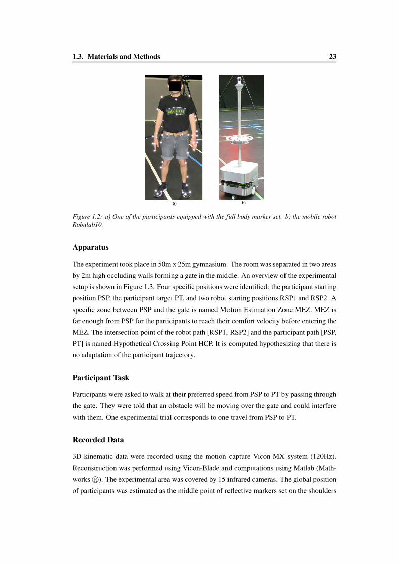
1.2 a) One of the participants equipped with the full body marker set. b) the
mobile robot Robulab10. . . . . . . . . . . . . . . . . . . . . . . . . . . . 23
1.3 Experimental apparatus and task. In this trial the robot was moving from
RSP1 to RSP2. Participant decided to pass behind the robot. . . . . . . . . 24
1.4 Representation of the tracking problem. . . . . . . . . . . . . . . . . . . . 27
1.5 Example of the analysis of one trial in which a switch of mpd sign occurred.
a) robot and pedestrian trajectories during the trial: triangles and star points
are their position at trob and tcross respectively. b) velocity profile of the
walker and the obstacle. c) mpd components. d) mpd evolution during
reaction phase (between trob and tcross). . . . . . . . . . . . . . . . . . . . 29
1.6 Example of the analysis of one of PosPos trials. . . . . . . . . . . . . . . . 29
1.7 smpd plots for all the 243 trials, after resampling over the interaction time
[trob, tcross]. . . . . . . . . . . . . . . . . . . . . . . . . . . . . . . . . . . 30
1.8 Three examples of participant-robot trajectories, for PosPos (a), PosNeg
(b) and NegNeg (c) category of trial. The part of the trajectory correspond-
ing to the interaction [trob, tcross] is bold. Time equivalent participant-
robot positions are linked by dotted line. . . . . . . . . . . . . . . . . . . . 31
1.9 (a) Mean evolution of smpd for each category of trial ±1 SD. (b) Time
derivative of the mean smpd. . . . . . . . . . . . . . . . . . . . . . . . . . 32
1.10 a) Comparison between initial and final values of smpd at trob and tcrossfor all trials of each non-empty category (PosPos, PosNeg, NegNeg). A
significant difference in values means that adaptations were made to the
trajectory by the participant (**p<0.01, ***p<0.001). b) Comparison be-
tween initial and final values of smpd at trob and tcross for all the trials of
each subgroup of the PosPos category. c) Total variation for smpd over
the interaction. d) Minimum distance observed between the robot and the
participant at tcross, with trial grouped by passing order of the participant. . 33

List of Figures ix
2.1 Experimental apparatus and task. The covered area was extended with
respect to the previous work. . . . . . . . . . . . . . . . . . . . . . . . . . 44
2.2 Experimental setup when robot is cooperative. The pedestrian moves from
PSP to the gate through the MEZ. At 0.67m before crossing the gate, the
actor is able to see the robot (tsee). In the following trial, the robot decel-
erates and passes behind the actor, going through VP1. The red robot and
the red actor illustrate the hypothetical crossing configuration. . . . . . . . 47
2.3 (a) smpd>0: The robot starts from RPS1, decelerates and turns right.
(b) smpd<0: the robot starts from RPS1, accelerates and turns left. (b)
smpd<0: the robot starts from RPS2, accelerates and turns right. . . . . . . 48
2.4 smpd plots for all the 278 trials, after resampling over the interaction time
[trob, tcross]. . . . . . . . . . . . . . . . . . . . . . . . . . . . . . . . . . . 50
2.5 Examples of participant and robot trajectories for each category of trial.
The bold trajectory represents the interaction time [trob, tcross]. . . . . . . . 51
2.6 Mean evolution of smpd ±1 Standard Deviation for the three categories
where the robot is passive. . . . . . . . . . . . . . . . . . . . . . . . . . . 52
2.7 smpd plots for all the 278 trials, after resampling over the interaction time
[tsee, tcross]. . . . . . . . . . . . . . . . . . . . . . . . . . . . . . . . . . . 54
2.8 Mean evolution of smpd ±1 the Standard Deviation (SD) for the three cat-
egories where the robot is cooperative. The category NegPos was not con-
sidered. . . . . . . . . . . . . . . . . . . . . . . . . . . . . . . . . . . . . 55
2.9 Examples of participant and robot trajectories for each category of trial.
The bold trajectory represents the interaction time [tsee, tcross]. . . . . . . . 56
3.1 General overview of the system architecture. . . . . . . . . . . . . . . . . 64
3.2 Illustration of important intermediate postures of the human behavior: step
with initiation of reaching, standing while opening of drawer, and reaching
for the object. . . . . . . . . . . . . . . . . . . . . . . . . . . . . . . . . . 65
3.3 Predictive planning of real human trajectories. Distances from the pelvis
to the front panel of the drawer (green, yellow and red), and the distance
between the front panel and the object (blue) for the ten trials (reproduced
from [Mukovskiy 2015a]). (b) The result of the re-targeting process: hu-
man avatar and HRP-2 robot during drawer opening task. . . . . . . . . . . 66
3.4 Extracted source signals. . . . . . . . . . . . . . . . . . . . . . . . . . . . 67
3.5 Architecture for the online synthesis of body movements using dynamic
primitives, [Giese 2009a]. This figure represents the module "Kinematic
Pattern Synthesis" (see page 74) . . . . . . . . . . . . . . . . . . . . . . . 68

x List of Figures
3.6 Scheme of the feedback loop used to control the humanoid robot HRP-2.
[vref ,ωref ] are respectively the linear and angular velocity and qupperbody
the upper body joint trajectories computed from the kinematic pattern syn-
thesis. q, q, q are respectively the generalized position and velocity vectors
computed using the Stack of Tasks (SoT). . . . . . . . . . . . . . . . . . . 74
3.7 (a) Off-line synthesized trajectories generated with the OpenHRP simulator. (b)
The humanoid robot HRP-2 in LAAS-CNRS during the experiments. . . . . . . . 75
3.8 Forces on the vertical axis (z) measured during the experiment. . . . . . . . 77
4.1 Objective: to steer a vehicle through a door using only visual measures.
The door is represented by two landmarks, FL and FR and the vehicle,
represented as a directed point, has an on-board camera and is subject to
nonholonomic constraints. . . . . . . . . . . . . . . . . . . . . . . . . . . 86
4.2 Elliptic coordinate system. Ellipses and hyperbolae intersect perpendicularly. 87
4.3 For any point Oc = (x, z) there always exists a circle Cα passing through
Oc and the projections in the motion plane of landmarks FL and FR. The
angle at the circumference α is constant along Cα. Notice that, the tangent
and perpendicular line inOc to the hyperbola throughOc, intersect theXW
axis in points A and B, respectively. The segment AB is the diameter of
circle Cα. . . . . . . . . . . . . . . . . . . . . . . . . . . . . . . . . . . . 92
4.4 The bipolar coordinate system consists of two orthogonal bundles of cir-
cles. Starting from the same point Oc, circle C⊥α crosses segment FLFR
in a point which is closer to the middle of the door than the one reachable
by following the hyperbola through Oc. . . . . . . . . . . . . . . . . . . . 93
4.5 Function F (τ, α) for different values of α and τ andK = 1. The minimum
is at the origin, i.e. at the middle of the door. . . . . . . . . . . . . . . . . . 96
4.6 Vector field obtained as the gradient of F (τ, α) with K = 1. . . . . . . . . 97
4.7 Trajectories of the vehicle starting from the same initial configuration q =(200,−50,7π/6), for different values of a in the control law: a = 40 cm
(the actual value), a= 80 cm (twice the actual value) and a= 20 cm (half
of the actual value). . . . . . . . . . . . . . . . . . . . . . . . . . . . . . . 100
4.8 Simulations with the feedback control law in elliptic coordinates: trajec-
tories of the vehicle without and with white Gaussian noise, representing
continuous and dashed lines, respectively. The vehicle leaves a room in (a),
(b) and enters a room from a corridor (c), by passing through a door. . . . . 101

List of Figures xi
4.9 Simulations with the feedback control law in bipolar coordinates: trajec-
tories of the vehicle with and without white Gaussian noise, representing
continuous and dashed lines, respectively. The vehicle leaves a room in (a),
(b) and enters a room from a corridor (c), by passing through a door. . . . . 102
4.11 Experimental setup. . . . . . . . . . . . . . . . . . . . . . . . . . . . . . . 103
4.10 PT7137 camera . . . . . . . . . . . . . . . . . . . . . . . . . . . . . . . . 103
4.12 Experimental results obtained applying the control law in elliptic coordi-
nates. The control parameters are w = 0.0012, K = 0.7 and λ = 310,
an the average linear velocity v = 0.3 m/s. . . . . . . . . . . . . . . . . . 108
4.13 Experimental results obtained applying the control law in bipolar coordi-
nates. The control parameters are K = 2, K1 = 4 and Kν = 0.15. Average
linear velocity of 0.4 m/s. . . . . . . . . . . . . . . . . . . . . . . . . . . . 109
4.14 Analysis of the FOV limits. . . . . . . . . . . . . . . . . . . . . . . . . . . 110
4.15 Some examples of trajectories with the same final orientation, generated by
the control laws in elliptic and bipolar coordinates and by Humans. In (a),
(b) and (c) the final orientation is 120 deg. (a) By elliptic coordinates. (b)
By bipolar coordinates. (c) By humans (from, [Arechavaleta 2008] cour-
tesy of the authors). . . . . . . . . . . . . . . . . . . . . . . . . . . . . . . 121
A.1 (a) The basic version of Robulab10 and (b) the one with the Pan–Tilt cam-
era PT7137 mounted on the top used for the experiments. . . . . . . . . . . 125

xii List of Figures

List of Tables
1.1 Organization of the trials. . . . . . . . . . . . . . . . . . . . . . . . . . . . 25
2.1 Organization of the trials . . . . . . . . . . . . . . . . . . . . . . . . . . . 45
2.2 Statistical analysis results of the smpd data during trob and tcross in the case
that the robot is passive. The Wilcoxon signed-rank test was performed
using Statistica v.8 . . . . . . . . . . . . . . . . . . . . . . . . . . . . . . . 51
2.3 Statistical analysis results of the smpd data during tsee and tcross in the case
that the robot is passive. The Wilcoxon signed-rank test was performed
using Statistica v.8 . . . . . . . . . . . . . . . . . . . . . . . . . . . . . . . 54
A.1 Main technical features of Robulab10. . . . . . . . . . . . . . . . . . . . . 125

xiv List of Tables

Introduction


3
F UTURISTIC visions of the world show humans and robots sharing the same envi-
ronment at different levels of interaction. Fifty years ago the idea that autonomous
systems could be active agents in the humans environment was just a dream realizable
only in movies. However, in the last decades the scientific community has done huge
improvements in this direction and robots are more and more integrated next to humans
for supporting them in different kinds of tasks. Recently, the robotics community started
to investigate what are the techniques to improve the performances of robots and, in
particular, their acceptance in the human society. Probably inspired by the past science
fictions, in which the robots had similar appearances and abilities than humans, scientists
started to believe that one way to increase robot capabilities was to endorse them with
human-like morphological characteristics and behaviors. For these reasons, an increasing
number of studies focus on the analysis and the identification of principles, invariants and
strategies used by a humans to daily interact with their environments. The development
of robots is improved by the progressive evolution of technology, allowing the realization
and control of more powerful and complex robots that look more and more like humans.
Nowadays the design of humanoid robots, able to help humans and work with them in a
real scenario, has became a very important scientific challenge.
The works described in this thesis are directed in such a direction. Assuming that the
planning of human movements is optimal, we wanted to study human behaviors during
walking tasks. Do we have implicit strategies when we interact with the surrounding
environment? Do we act differently each time we have to avoid an obstacle or do we use
implicit principles? What are the rules that drive us when we have to walk in a constrained
environment like passing through a door? Can we identify and model them? When humans
perform a simple action, is it really "simple" or is it made up with hierarchical sequence
of sub-tasks? During this thesis we addressed these questions, basing our studies on the
analysis of human walking behavior in different situations, with the aim of identifying the
invariants of human movements and transfer them to robots.
A large part of the work done in this thesis was done within the framework of the
European project KoroiBot. The aim of this project was to improve walking motions of
humanoid robots in different scenarios, providing software tools based on mathematical
models and methods, in particular optimization, and learning from human data. A more
detailed description of the project is provided in the following section.

4 Introduction
The European Project KoroiBot
Figure 1: Project components of KoroiBot and Interdisciplinary foundations.
The goal of the KoroiBot project is to enhance the ability of humanoid robots to walk
in a dynamic and versatile fashion in the way humans do. Research and innovation work
in KoroiBot mainly targets novel motion control methods for existing hardware, but also
derives optimized design principles for next generation robots. The new software technolo-
gies are based on biological data, with the aim of increasing the performance of humanoid
walking. Especially for humanoid robots with redundant degrees of freedom (DoF), opti-
mization and learning might be solutions to make the redundancy a benefit rather than a
burden. As depicted in Fig. 1, the project methodology can be divided into four pillars:
(1) investigation of human walking by experiments, and related extraction of motion prim-
itives by mathematical models and identification of walking principles; (2) development of
adequate transfer rules; (3) development of novel optimization and learning based control
approaches for humanoids walking, (4) integration of these algorithm on several robots
(see Fig. 2). In order to test and evaluate the developed software, an interesting scenario
consisting of different challenges for the humanoid robots was proposed (Fig. 3).

5
Figure 2: The seven humanoid robot platforms of the KoroiBot consortium dreaming of humanwalking capabilities.
Figure 3: Challenges of the KoroiBot project. In red the challenges addressed by the LAAS-CNRS.

6 Introduction
The work in the KoroiBot context
The European project KoroiBot is an interdisciplinary project. Each partner was assigned
to different work packages (WP) focused on particular studies, as shown in Fig. 4. Among
these WPs the work that I did during my thesis is related to WP1 and WP2. The former
consisted to make different experiments for recording human walking data, aimed at
the modeling and the developing of novel motion control laws inspired by biology. The
latter targets to synthesize complex actions from sequences of elementary motor tasks and
transfer them to the humanoid robots of the consortium.
Figure 4: Pert chart of the KoroiBot work packages and their interrelationships Our studies con-cerned WP1 and WP2.

7
Overview of the thesis
The work presented in this thesis is mainly focused on the analysis of human motion and
the identification of human principles that can be transferred to robots for improving their
capabilities. The manuscript can be roughly divided in two parts: the first one describes the
studies that have been done in the context of the KoroiBot project. The second part presents
a collaboration that has been done internally at LAAS-CNRS. The thesis is divided in four
main chapters that can be summarized as follows:
ä Chap. 1 and 2 : Identification of walking strategies for avoiding a moving obstacle,
ä Chap. 3 : Use of motion primitives to implement complex movements on humanoid
robots,
ä Chap. 4 : Vision-based control to pass through a door.
An overview of each chapter is provided in the following sections.
Chapter 1
Title: How humans avoid moving obstacle crossing their way?Study: Identification of walking strategies for avoiding a moving obstacle
Context: KoroiBot project, WP1
Time: during 1st and 2nd year
Collaborators: INRIA-Rennes, MimeTIC research team
and University of Rennes 2, M2S lab
People: Anne-Hélène Olivier, Julien Pettré and Armel Crétual
Place: LAAS-CNRS (Toulouse) and Campus de Ker Lann (Rennes)
Key Words: Human direct-goal locomotion, Motion Capture System,
Moving obstacle, Collision avoidance strategies, Passive Behavior
Summary
One of the first steps of this thesis was to analyze human walking motions during situa-
tions which could perturb the natural behavior of a person. With this aim, we decided to
make experiments in which a pedestrian, that was walking calmly and naturally, was sig-
nificantly disturbed. To this end, we wanted to introduce one or multiple external agents in
the scenario, as obstacles, in order to record human reactions in terms of trajectory (speed
and turning) and body organization (orientation of the feet, shoulders, head and the step
frequency). In order to generate such a situation, the "obstacle" had to move. In particular,
as we wanted to create precise and repeatable experiments, we chose to control a wheeled

8 Introduction
robot to impersonate the moving obstacle. Having in mind the related works on human
locomotion, we found interesting the possibility to collaborate with specialists in this field.
So, we started a productive partnership with researchers of INRIA-Rennes who, in their
previous studies, had investigated the strategies set by two humans crossing each other or
in a crowd scenario. In particular, the main idea was to compare the human strategies that
our partners already identified, with the ones set to avoid a moving obstacle. Given their
experience in human motion and our knowledge in robot control, we setup interesting ex-
periments in which a moving obstacle had to perpendicularly cross the pedestrian path. The
control algorithm allowed us to generate specific interactions that aimed to be as similar as
possible to the ones observed between two humans. All the experiments took place in the
Campus de Ker Lann which provides a huge gymnasium supplied with a motion capture
system that perfectly matched our objectives. The recorded human data have been shared
and uploaded in the KoroiBot database. After several tests we realized the ideal experimen-
tal setup: the robot starting position had to be hidden by some occluding walls otherwise
the pedestrians were adapting too early; moreover, the wheeled robot had to be a fast and a
robust object in order to perturb significantly the behavior of the participants. To help the
reader to figure out the scenarios, an overview of them is shown in Fig. 5. In the following
chapter, we will present experiments where the moving obstacle was controlled to behave
passively (1). In this way, only the participant contributed to solve the collision.
Figure 5: An overview of two different scenarios tested in this study. In the left picture, two Turtle-Bots dressed with some papers to make them look bigger. The participant had to walk straightand avoid them. In the right picture, we improved the experimental setup introducing some oc-cluding walls and considering the wheeled robot Robulab that is faster and looks heavier. Eachexperimental setup, required at least one week of work to be realized and calibrated.
Passive Behavior (1)
In this manuscript we use the term "Passive Behavior" to indicate that the robot was
controlled to move straight and at constant speed. The robot was not reacting to the
adaptations performed by the participants.
9
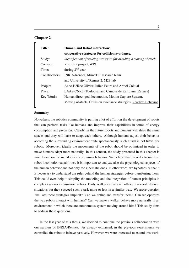
Chapter 2
Title: Human and Robot interaction:cooperative strategies for collision avoidance.
Study: Identification of walking strategies for avoiding a moving obstacle
Context: KoroiBot project, WP1
Time: during 3rd year
Collaborators: INRIA-Rennes, MimeTIC research team
and University of Rennes 2, M2S lab
People: Anne-Hélène Olivier, Julien Pettré and Armel Crétual
Place: LAAS-CNRS (Toulouse) and Campus de Ker Lann (Rennes)
Key Words: Human direct-goal locomotion, Motion Capture System,
Moving obstacle, Collision avoidance strategies, Reactive Behavior
Summary
Nowadays, the robotics community is putting a lot of effort on the development of robots
that can perform tasks like humans and improve their capabilities in terms of energy
consumption and precision. Clearly, in the future robots and humans will share the same
spaces and they will have to adapt each others. Although humans adjust their behavior
according the surrounding environment quite spontaneously, such a task is not trivial for
robots. Moreover, ideally the movements of the robot should be optimized in order to
make humans adapt more naturally. In this context, the study presented in this chapter is
more based on the social aspects of human behavior. We believe that, in order to improve
robot locomotion capabilities, it is important to analyze also the psychological aspects of
the human behavior and not only the kinematic ones. In other word, we hypothesize that it
is necessary to understand the rules behind the human strategies before transferring them.
This could even help to simplify the modeling and the integration of human principles in
complex systems as humanoid robots. Daily, walkers avoid each others in several different
situations but they succeed such a task more or less in a similar way. We arose question
like: are these strategies implicit? Can we define and transfer them? Can we optimize
the way robots interact with humans? Can we make a walker behave more naturally in an
environment in which there are autonomous system moving around him? This study aims
to address these questions.
In the last year of this thesis, we decided to continue the previous collaboration with
our partners of INRIA-Rennes. As already explained, in the previous experiments we
controlled the robot to behave passively. However, we were interested to extend this work,

10 Introduction
by controlling the robot in a more unpredictable way to perturb more considerably the
innate walking of the pedestrians. To this end, in this second part we controlled the robot
to behave reactively (2). We transferred the collision avoidance strategies observed in
humans to the robot and we analyzed the human reactions. The main idea was to study
the differences with respect to the case in which the robot behaves passively. Moreover,
we wanted also to compare the avoidance strategies of the participants, in the case that
the robot acts like a human, with respect to the ones observed between two pedestrians
[Olivier 2013]. We reproduced the same experimental setup of the Chap. 1, improving the
quality and the design of the experiments. We used the same robot platform. An overview
of the scenario is shown in Fig. 6.
Figure 6: An overview of the experimental setup of the study presented in Chap. 2.
Reactive Behavior (2)
In this manuscript we use the term "Reactive Behavior" (or "Active Behavior")
to indicate that the robot was controlled to positively contribute to the collision
avoidance. In reactive mode, the robot predict human movements and it adapts its
velocity and orientation in order to avoid the collision.

11
Chapter 3
Title: Learning Movement Primitives for the Humanoid Robot HRP-2Study: Use of motion primitives to implement complex movements
on humanoid robots
Context: KoroiBot project, WP2
Time: during 2nd and 3rd year
Partners: University Clinic Tübingen, Department of Cognitive Neurology
People: Albert Mukovskiy, Martin A. Giese
Place: LAAS-CNRS (Toulouse)
Key Words: Robotics, Goal-directed walking, Motion primitives,
Walking pattern generator, Motor coordination, Action sequences
Humanoid robots are complex and redundant mechanical systems. One of the robotics
community challenges is to create humanoid robots equipped with human features
i.e. communication skills, walking capabilities, adaptation and reactive movements.
However, humans and humanoid robots are really different in terms of size, geometrical
proportions, velocity and acceleration limits, power and energy consumption. Human
abilities are learned and improved by life experience and they are further improved
everyday. For this reason, it is really challenging to find the way to transfer such advanced
human capabilities to robots. However, recent studies on human motion have shown that
complex actions can be represented as a sequence of motor primitives (3) [Flash 2005].
These motion primitives are hypothesized as being the "building bricks" of any action.
Therefore, the main idea is that instead of analyzing and trying to reproduce human
full-body complex motion, one should identify the "alphabet" of movements used by the
brain. In other words, assuming that an alphabet of movements is known, it could be
possible to compose any kind of complex movements as a sequence of contribution of
simple letters that are the motion primitives.
In the framework of the KoroiBot project, the WP2 proposed to integrate complex
motion strategies into locomotion control as simple sequences of individual steps or step
phases, which mimic optimal behavior of humans. Based on some extracted primitives,
techniques as machine learning and optimal control should be used to derive models
and data, and transfer them to humanoid robots. In this context, we decided to consider
walking-to-grasp movements and implement them on the humanoid robot HRP-2 at
LAAS-CNRS.

12 Introduction
In this chapter we will present a novel highly flexible approach to model complex
movements based on an hierarchical use of motion primitives. These primitives can be
combined in space and time and over multiple temporal scales. They are learned by bio-
logical kinematic data and then reformulated in a mathematical framework which allows
their implementation in optimal control systems. The methods we used for learning the
motion primitives are based on previous works done by our partners from Tübingen. They
allow to decompose complex movements in terms of motion primitives, based on kinematic
data [Giese 2009b, Mukovskiy 2013]. In this context, we proposed a whole body controller
in which the upper-body movements are generated by a combination of such motion prim-
itives whereas the lower body behavior is computed by a walking pattern generator.
Figure 7: An illustrated overview of the work presented in Chap. 3. In the left, an avataris reproducing some movements recorded from a human. In the center, an avatar of thehumanoid robot HRP-2 is performing the same movements but in a realistic simulation. Inthe right, a snapshot of real experiments done with the robot HRP-2 at LAAS-CNRS.
Motion Primitives (3)
"Motion Primitives" (or "Motor Primitives") refer roughly to building blocks at
different levels of the motor hierarchy. They do need to be universal and the same
building block is not necessarily used for all the possible behaviors or tasks. Instead,
they might be specific to only a particular representation of movements or tasks.
The crucial feature is that many different movements can be derived from a limited
number of motor primitives through appropriate operations and transformations,
and that these movements can be combined through a well defined syntax of motion
to generate more complex actions. An exhausting description of Motion Primitives,
at different levels (behavioral, neural, muscle, kinematic and dynamic), has been
provided by Tamara Flash [Flash 2005]

13
Chapter 4
Title: The geometry of confocal curves for passing through a doorStudy: Vision-based control to pass through a door
Context: Internal collaboration (LAAS-CNRS)
Time: during 1st and 2nd year
Collaborator: ERC Actanthrope
People: Paolo Salaris, Jean-Paul Laumond
Place: LAAS-CNRS (Toulouse)
Key Words: Nonholonomic motion planning, Visual servoing, Wheeled robots
From the experience gained and the software developed to control a wheeled robot as a
moving obstacle, we developed an internal collaboration at LAAS-CNRS within the frame-
work of ERC Actanthrope. The aim of this work was to implement some vision-based
control laws to steer a robot through a door by using advanced geometric parametriza-
tion provided by confocal curves. At the beginning we planned to implement this control
on HRP-2, however given the difficulties to obtain accurate vision-based controls during
walking on humanoid robots, we decided to initially test the algorithm into a nonholonomic
wheeled robot equipped with a rigidly pinhole camera. We developed and implement con-
trol strategies to detect a door, identified by two landmarks attached to its vertical supports,
and steer the vehicle to pass through it. We built around the door a planar geometry of
bundles of hyperbolas, ellipses and orthogonal circles. The method is able to drive the
robot to the goal by using static feedback control laws that are function of the current state
of the system expressed in suitable coordinates. The originality of this work is that these
new coordinates can be directly measured in the camera plane. Although the methods
was implemented on a wheeled robot and not an anthropomorphic system, we found that
the proposed approach had similarities with the strategy adopted by humans for passing
through a door. An overview of the experimental setup is depicted in Fig. 8.
FRFLRobulab 10
On-board camera
Robulab 10
Door
DoorFR FL On-board camera
From behind the door
Figure 8: An overview of the experimental setup of the work shown in Chap. 4. The wheeled robotis the same as the one used for the works presented in Chap. 1– 2. The entire work was done atLAAS-CNRS.

14 Introduction
Other contributions
During the three years of my thesis I also had some other minor contributions. They are
rapidly described in this introduction but not further developed in the manuscript.
Recording human motion in the KoroiBot scenario
In the context of the Koroibot WP1, we participated with our project partners from
University of Tübingen and University of Heidelberg to experiments for recording human
movements in the KoroiBot scenario previously shown in Fig. 3. In all the experiments
the body kinematics was recorded with 10 Vicon-MX cameras and the normal forces
under the feed was collected with Pedar System. The participants were told to perform
the following tasks: walking straight, walking stairs up and down forwards, walking on a
soft mattress, walking on a beam forwards, walking on different slopes fast up and down,
stepping stones with two different configurations, walking following a circular trajectory
at different speed. An overview of the experiments is shown in the pictures above. An
illustration of some experiments is provided in Fig. 9.
Figure 9: Illustration of four different tasks. From top-left to bottom-right: walking on a softmattress, walking on a beam, stepping stones, walking stairs up. The kinematic data and the relatednormal forces are depicted in the smaller images.

15
A new tool for tracking HRP-2 with the motion capture system of LAAS-CNRS
Another minor contribution during this thesis has been done at the beginning of the first
year. Supported by Airbus/Future of Aircraft Factory and CNRS, we presented a prelim-
inary proof of concept aiming at introducing humanoid robots in an aircraft factory. The
goal was to demonstrate the capabilities of HRP-2 to deal with three aspects needed in a
factory: reactivity to the changes of the environment, visual feedback and on-line motion
generation. In particular, the robot had to move from a random starting position to a prede-
fined target, while avoiding a moving obstacle crossing its way (respectively the red pylon
engine depicted in blue and the red moving toolbox in Fig. 10). In order to localize the
position of the robot, the obstacle and the target in the environment, each of them were
equipped with markers and tracked by a motion capture system (MoCap) in the area. My
contribution was to find the transformation matrix that links the HRP-2 joint frames and
the MoCap system. In other words, we determined a tool to express the position and the
orientation of each joint frame of HRP-2 in the MoCap frame. Thanks to this tool, that it
is still currently used, we have been able to make improvements for our laboratory setup.
For example, it has been possible to implement an algorithm into the crane control system
for an automatic tracking and following of the robot during the experiments in the area.
Moreover, we used this tool also for the benchmark of KoroiBot. Through motion cap-
ture system, we evaluate the precision and the improvement of HRP-2 walking controls,
comparing the expected configurations and the real ones in different trials of walking.
Figure 10: (Left) The robot is moving according to the position of the red pylon engine in order tomaintain the same distance (1 meter). (Right) Situation of the experiment: the robot has to go inthe vicinity of the pylon engine, depicted in blue, avoiding the red moving toolbox. The robot hasto re-plan its path in real-time. In both cases, the robot is tracking the objects using the motioncapture system.

16 Introduction
Publications
Journal
Accepted
n C. Vassallo, AH. Olivier, P. Souères, A. Crétual, O. Stasse et Pettré J. How do walkers
avoid a mobile robot crossing their way? Gate and Posture, vol. 51, pages 97 – 103,
2017
n P. Salaris, C. Vassallo, P. Souères et JP. Laumond. The geometry of confocal curves
for passing through a door. IEEE Transactions on Robotics, vol. 31, no. 5, pages
1180–1193, 2015
Under review
n A. Mukovskiy, C. Vassallo, M. Naveau, O. Stasse, P. Souères et MA. Giese. Adap-
tive synthesis of dynamically feasible full-body movements for the Humanoid Robot
HRP-2 by flexible combination of learned dynamic movement primitives. Robotics
and Autonomous Systems, 2016. Corrected version under review
Conference
Accepted
n P. Salaris, C. Vassallo, P. Souères et J-P. Laumond. Image-based control relying
on conic curves foliation for passing through a gate. In 2015 IEEE International
Conference on Robotics and Automation (ICRA), pages 684–690. IEEE, 2015
n O. Stasse, F. Morsillo, M. Geisert, N. Mansard, M. Naveau et C. Vassallo. Air-
bus/future of aircraft factory HRP-2 as universal worker proof of concept. In 2014
IEEE-RAS International Conference on Humanoid Robots, pages 1014–1015. IEEE,
2014
n A Mukovskiy, C. Vassallo, M. Naveau, O. Stasse, P. Souères et Giese MA. Learning
Movement Primitives for the Humanoid Robot HRP-2. In IEEE IROS 2015 Work-
shop on "Towards truly human-like bipedal locomotion: the role of optimization,
learning and motor primitives". Hamburg, Germany, 2015

CHAPTER 1
How humans avoid moving obstaclecrossing their way?

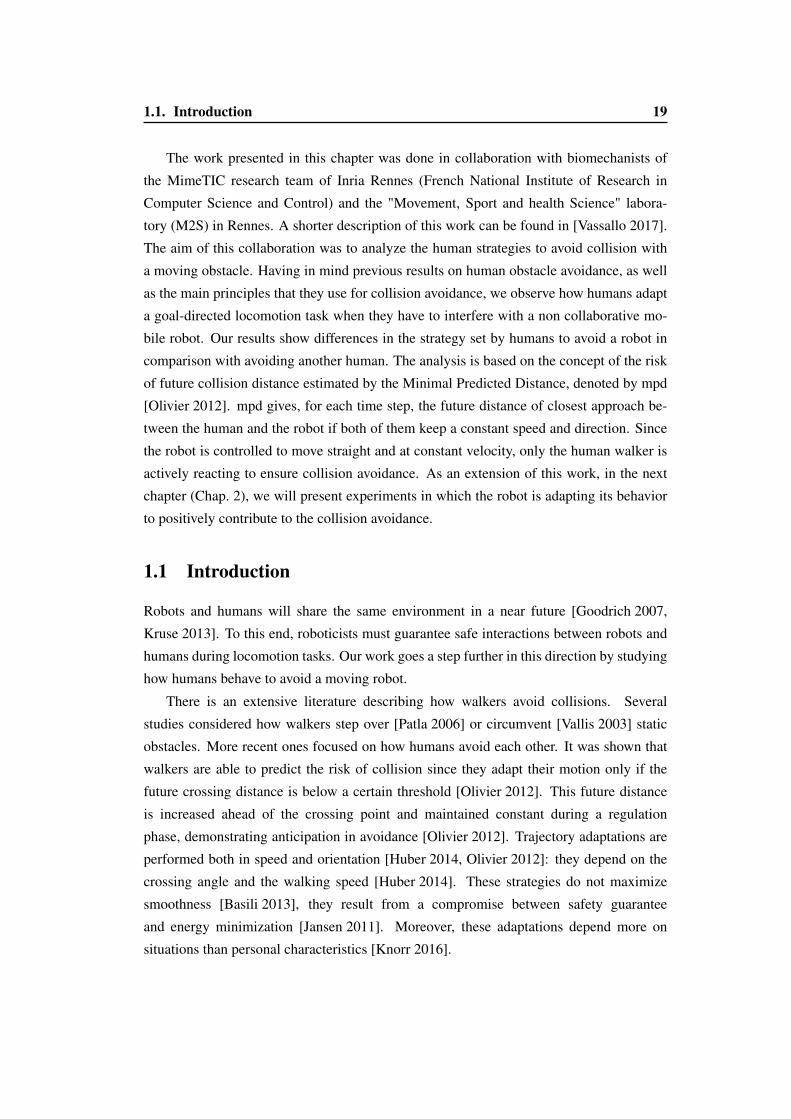
1.1. Introduction 19
The work presented in this chapter was done in collaboration with biomechanists of
the MimeTIC research team of Inria Rennes (French National Institute of Research in
Computer Science and Control) and the "Movement, Sport and health Science" labora-
tory (M2S) in Rennes. A shorter description of this work can be found in [Vassallo 2017].
The aim of this collaboration was to analyze the human strategies to avoid collision with
a moving obstacle. Having in mind previous results on human obstacle avoidance, as well
as the main principles that they use for collision avoidance, we observe how humans adapt
a goal-directed locomotion task when they have to interfere with a non collaborative mo-
bile robot. Our results show differences in the strategy set by humans to avoid a robot in
comparison with avoiding another human. The analysis is based on the concept of the risk
of future collision distance estimated by the Minimal Predicted Distance, denoted by mpd
[Olivier 2012]. mpd gives, for each time step, the future distance of closest approach be-
tween the human and the robot if both of them keep a constant speed and direction. Since
the robot is controlled to move straight and at constant velocity, only the human walker is
actively reacting to ensure collision avoidance. As an extension of this work, in the next
chapter (Chap. 2), we will present experiments in which the robot is adapting its behavior
to positively contribute to the collision avoidance.
1.1 Introduction
Robots and humans will share the same environment in a near future [Goodrich 2007,
Kruse 2013]. To this end, roboticists must guarantee safe interactions between robots and
humans during locomotion tasks. Our work goes a step further in this direction by studying
how humans behave to avoid a moving robot.
There is an extensive literature describing how walkers avoid collisions. Several
studies considered how walkers step over [Patla 2006] or circumvent [Vallis 2003] static
obstacles. More recent ones focused on how humans avoid each other. It was shown that
walkers are able to predict the risk of collision since they adapt their motion only if the
future crossing distance is below a certain threshold [Olivier 2012]. This future distance
is increased ahead of the crossing point and maintained constant during a regulation
phase, demonstrating anticipation in avoidance [Olivier 2012]. Trajectory adaptations are
performed both in speed and orientation [Huber 2014, Olivier 2012]: they depend on the
crossing angle and the walking speed [Huber 2014]. These strategies do not maximize
smoothness [Basili 2013], they result from a compromise between safety guarantee
and energy minimization [Jansen 2011]. Moreover, these adaptations depend more on
situations than personal characteristics [Knorr 2016].

20 Chapter 1. How humans avoid moving obstacle crossing their way?
The crossing order during collision avoidance is an interesting parameter to con-
sider. Indeed, it has been shown that trajectory adaptations are collaboratively performed
[Olivier 2012] but are role-dependent. The walker giving way (2nd at the crossing) con-
tributes more than the one passing first. This role attribution appears to contribute pos-
itively before the interaction [Knorr 2016, Olivier 2013] and can be predicted with 95%
confidence at almost 2.5m before crossing, even before any adaptation [Knorr 2016].
Studies resulted into simulation models of navigation and interaction. Warren and Fa-
jen [Warren 2008] proposed to model the walker and the environment as coupled dynamical
systems: the walker paths result from all the forces acting on them, where goals are consid-
ered as attractors and obstacles as repellors. This model is based on the distance to the goal
and to the obstacles as well as the sign of change of the bearing angle. An integration of the
bearing angle theory into some artificial vision system for crowd simulation was proposed
by Ondrej et al. [Ondrej 2010].
These previous studies reached common conclusions about the human ability to
accurately estimate the situation (crossing order, risk of collision, adaptations), and
considered interactions with a moving objects. The kinematics of adaptations by a
walker avoiding a moving obstacle (a mannequin mounted on a rail) are studied in
[Cinelli 2007, Cinelli 2008, Gérin-Lajoie 2005]. Trajectories crossing at 45◦ resulted into
adaptations both in the antero-posterior and medio-lateral planes, with successive anticipa-
tion and clearance phases [Gérin-Lajoie 2005]. Analysis is based on the notion of personal
space modeled as a free elliptic area around each walker. When trajectories are colinear
(the mannequin comes from the front), a 2-step avoidance strategy is observed: participants
first adapt their locomotion in heading, then by speed [Cinelli 2008]. Moreover, the obsta-
cle velocity influences the lateral rate of change of the walker trajectory [Cinelli 2007];
the slower the velocity, the lower the lateral rate of change. These experiments with man-
nequins were not designed to study the question of the crossing order. Other studies in-
vestigated human interactions with robots. It was shown that it is easier to understand and
predict the behavior of robots if they are human-like [Carton 2013, Lichtenthäler 2013].
Some studies demonstrated that human-like behaviors [Dragan 2015, Kato 2015] improve
on many levels the performance of human-robot collaboration. Nevertheless, the benefit
of programming a robot with human-like capabilities to move and avoid collision with a
human walker has not been demonstrated yet.
The chapter is structured as follows. Firstly, we recall the meaning of Minimal Pre-
dicted Distance. Then we present our approach in which a moving robot has to interfere
with a pedestrian. The experimental setup is detailed in Section 1.3. In Section 1.4 we
show how to control the robot to reproduce similar kinematic condition of interaction than
the ones studied in [Olivier 2012] (in terms of relative angle, position, and velocities) and

1.2. Minimal Predicted Distance 21
we apply a similar analysis in Section 1.5. While the nature of the interaction is changed,
our results show differences in the strategy set by humans to avoid a robot in comparison
with avoiding another human (Section 1.6 and Section 1.7). Finally we will see in Sec-
tion 1.8 how humans prefer to give the way to the robot even when they are likely to pass
first at the beginning of the interaction.
1.2 Minimal Predicted Distance
As explained before, the crossing configuration and the risk of future collision were esti-
mated by the Minimal Predicted Distance, noted mpd [Olivier 2012]. In other world, the
mpd functions provides information about the risk of collision: the smaller the mpd, the
higher the risk of collision. For each time step, its value correspond to the future distance of
closest approach if both the robot and the participant keep a constant speed and direction.
Thus, as the robot is moving straight at constant speed (in the time phase of the experi-
ments which are presented in this chapter), a variation of mpd means that the participant is
performing adaptations. In other words, collision avoidance could be analyzed with respect
to the variation of speed v and the orientation θ during the reaction phase (see Figure 1.1).
In order to identify what were the main adaptations (accelerating/decelerating or turning),
we partially derived the mpd function. Indeed, denoting by θ1 and s1 the instantaneous
orientation and speed of participant #1 (θ2 and s2 for #2 respectively) and X = (a,b) the
relative position of participant #2 with respect to #1, the mpd turns on to be a function of
all these variables:
mpd= f(a,b,θ1,s1,θ2,s2) (1.1)
For any of the 6 parameters ∈ {a,b,θ1,s1,θ2,s2}, the instantaneous individual effect of p,
in the mpd, can be expressed by the following partial derivative:
εp = ∂mpd
∂p·dp= ∂f
∂p·dp (1.2)
The total instantaneous effect5f of the 6 parameters is then:
5f = εa+εb+εθ1 +εθ2 +εv1 +εv2 (1.3)
As an extension of the previous works [Olivier 2012, Olivier 2013], we introduced a signed
definition of the mpd, noted smpd. The sign of this function depends on who, among the
human and the robot, is likely to pass first or give way to the other participant. Further
details will be treated in Section 1.5.

22 Chapter 1. How humans avoid moving obstacle crossing their way?
Figure 1.1: Illustration of the mpd evolution during the reaction phase between two humans cross-ing each other [Olivier 2012]. We defined tsee as the instant of time in which the participant startsto see the other one, and tcross as the crossing time. From the picture, we observe that the mpd attsee is around 0.32m, that means the participants will not collide but they are going to pass near toeach other. Once the Reaction phase starts, the mpd is increasing because one of the participants(or perhaps both of them) is reacting to increase the future distance at tcross. In the end of thereaction phase, the mpd is around 0.7m.
1.3 Materials and Methods
Participants
Seven volunteers participated in the experiment (1 woman and 6 men). They were 26.1
(± 5.4) years old and 1.78m tall (±0.21). They had no known vestibular, neurological or
muscular pathology that would affect their locomotion. All of them had normal or corrected
sight and hearing. Participants gave written and informed consent before their inclusion in
the study. The experiments respect the standards of the Declaration of Helsinki (rev. 2013),
with formal approval of the ethics evaluation committee Comitè d’Evaluation Ethique de
l’Inserm (IRB00003888, Opinion number 13-124) of the Institut National de la Santé et
de la Recherche Médicale, INSERM, Paris, France (IORG0003254, FWA00005831). All
the participants were equipped with a full body marker set (53 markers) (see Figure 1.2a).
They were located following the standard marker placement of Koroibot project 1.
1https : //koroibot−motion−database.humanoids.kit.edu/markerset/
1.3. Materials and Methods 23
Figure 1.2: a) One of the participants equipped with the full body marker set. b) the mobile robotRobulab10.
Apparatus
The experiment took place in 50m x 25m gymnasium. The room was separated in two areas
by 2m high occluding walls forming a gate in the middle. An overview of the experimental
setup is shown in Figure 1.3. Four specific positions were identified: the participant starting
position PSP, the participant target PT, and two robot starting positions RSP1 and RSP2. A
specific zone between PSP and the gate is named Motion Estimation Zone MEZ. MEZ is
far enough from PSP for the participants to reach their comfort velocity before entering the
MEZ. The intersection point of the robot path [RSP1, RSP2] and the participant path [PSP,
PT] is named Hypothetical Crossing Point HCP. It is computed hypothesizing that there is
no adaptation of the participant trajectory.
Participant Task
Participants were asked to walk at their preferred speed from PSP to PT by passing through
the gate. They were told that an obstacle will be moving over the gate and could interfere
with them. One experimental trial corresponds to one travel from PSP to PT.
Recorded Data
3D kinematic data were recorded using the motion capture Vicon-MX system (120Hz).
Reconstruction was performed using Vicon-Blade and computations using Matlab (Math-
works r). The experimental area was covered by 15 infrared cameras. The global position
of participants was estimated as the middle point of reflective markers set on the shoulders

24 Chapter 1. How humans avoid moving obstacle crossing their way?
Figure 1.3: Experimental apparatus and task. In this trial the robot was moving from RSP1 toRSP2. Participant decided to pass behind the robot.
(acromion anatomical landmark, LSHO-RSHO). The stepping oscillations were filtered out
by applying a Butterworth low-pass filter (2nd order, dual pass, 0.5Hz cut-off frequency).
Experimental plan
Each participant performed 40 trials (see Table 1.1). Robot starting position (50% in RSP1,
50% in RSP2) was randomized among the trials. To introduce a bit of variability, in 4 trials
the robot did not move and the participant did not have to react. Only the 36 trials with
potential interaction were analyzed.
Robot Behavior
We used a prototype of RobuLAB10 wheeled robot from the Robosoft company (dimen-
sion: 0.45 x 0.40 x 1.42m, weight 25 Kg, maximal speed around 3 m/s) (see Figure 1.2b).
The robot position was detected as the center point in its base (more details are given in

1.3. Materials and Methods 25Table 1.1: Organization of the trials.
Trial Robot Moving RSP MPD Trial Robot Moving RSP SMPD1 Yes Right 0.8 21 Yes Left -0.12 Yes Left 0.8 22 No Left – –3 Yes Right 0 23 Yes Right 0.14 Yes Right 0.1 24 Yes Left 0.15 Yes Right 1.2 25 Yes Left -0.86 No Right – – 26 Yes Left 1.27 Yes Left 0.1 27 Yes Left -0.38 No Right – – 28 Yes Left 1.29 Yes Right -0.3 29 Yes Right 0.8
10 Yes Left 0.3 30 Yes Right 0.311 Yes Left -0.3 31 Yes Right -0.112 Yes Left 0 32 Yes Left 013 Yes Left 0.8 33 Yes Left -0.114 Yes Right 0 34 Yes Right 1.215 Yes Left -1.2 35 Yes Right 0.316 Yes Left -1.2 36 Yes Left 0.317 Yes Right -1.2 37 Yes Left -0.818 No Left – – 38 Yes Right -0.819 Yes Right -0.8 39 Yes Right -0.120 Yes Right -0.3 40 Yes Right -1.2
Section 1.4). We programmed the robot to execute a straight trajectory between RSP1 and
RSP2 at constant speed (1.4 m/s). The robot was controlled to generate specific interac-
tions with the participant. In particular, the robot was either: a) on a full collision course
(reach HCP at the same time than the participant), b) on a partial collision course (the robot
reaches HCP slightly before or after the participant), or c) not on a collision course. To this
end, we measured the participants speed through MEZ and estimated the time thcp at which
HCP was reached. We deduced the time trs at which the robot should start to reach HCP at
thcp. We finally added an offset 4t to trs in order to obtain the desired interactions based
on mpd values selected from the range [-1.2m, 1.2m]. Although the sequence of interac-
tions was pre-defined in the remote control station (see Table 1.1), the participants were
unaware about it. Each trial was repeated twice.
At the beginning of each trial, the software read the respective line of the table above.
The robot starting position was initialized based on the robot velocity (set as constant) and
the walker speed. To estimate the latter we used a Kalman Filter, modeling the walker
as a material point moving along a line at constant speed (no acceleration). Tests have
shown that participant velocity was almost constant in MEZ, then such an approximation
was sufficient to reliably estimate the gait speed.

26 Chapter 1. How humans avoid moving obstacle crossing their way?
1.4 Obstacle Control
The robot position was tracked using a Vicon motion capture system. The robot position
was computed as the centroid of seven markers fixed on its base. The remote control
station was an external computer, communicating with the robot platform and the motion
capture software through Wi-Fi. The exchange of data between the control station and the
Vicon system was established by the ROS Hydro package vicon_bridge 2 which contains
the driver needed for the communication. The robot was controlled by the remote station
though an UDP connection. Further details about the low-level control of the robot Robulab
are provided in Appendix A.
An overview of the experiment was shown in the previous section. The participant had
to walk straight, from PSP to PT, pass through the gate and avoid a moving obstacle. The
middleware ROS Hydro was used to interface the robot with the motion capture system and
the remote control station. In order to guarantee accuracy and reliability of the experiments,
a virtual robot with reference behavior was defined to plan the collision. Since obstacle
velocity was set as constant (1.4 m/s), the initial position of the virtual robot changed
according to the walker gait speed. In other words, the mobile obstacle was controlled
in order to follow precisely the behavior of a virtual robot designed to obtain the desired
crossing situation. Tracking control was considered for this task.
A right-handed reference frame W with origin in Ow and axes Xw and Yw is attached
to the plane of the robot motion. The configuration of the vehicle is described by q(t) =(x(t),y(t),θ(t)), where (x(t),y(t)) is the position in W of a reference point of the vehicle
and θ(t) is the orientation with respect to Xw. Denoting by v(t) and ω(t) the forward and
angular velocities, the kinematics is:
x
y
θ
=
cosθ 0sinθ 0
0 1
vω
(1.4)
The tracking problem, under the assumption that the robot velocity never vanishes, is to
find a feedback control law such that the configuration q(t) of the real robot matches the
one qr(t) of the virtual robot. The error e(t) = q(t)− qr(t) can be written as:
e=
e1
e2
e3
=
cosθ sinθ 0−sinθ cosθ 0
0 0 1
xr−xyr−yθr−θ
(1.5)
2http : //wiki.ros.org/vicon_bridge

1.4. Obstacle Control 27
Figure 1.4: Representation of the tracking problem.
In [Zheng 1994] the authors have proposed the follows change of inputs
u1 =−v+vr cose3
u2 = ωr−ω
and proved that the following nonlinear feedbacks make the error q(t)− qr(t) converge to
zero
u1 =−k1(vr,ωr)e1
u2 =−k4vrsine3e3
e2−k3(vr,ωr)e3
where k4 is a positive constant and k1,k3 are continuous functions of vr and ωr, strictly
positive. The starting point of the virtual robot changed according to the gait speed of the
actor. Considering s as the distance between RSP and HCP, and vg as the average walking
speed of the participant, it is possible to determine the time needed by the walker to reach
HCP (tcross). Defining this interval as Time To Contact TTC, we obtain:
TTC = s+mpd
vg(1.6)
Since the robot needs time to reach a constant velocity, it was starting to move before the
participant crossed the gate. In this way, the obstacle was perceived to move at constant
speed. In order to guarantee that the tracking was feasible, the following condition needed
to be satisfied: if the virtual robot was slightly ahead to the real one, the latter started to
follow the former. Without this control, the real robot was moving backward. However,
a considerable acceleration was required at the beginning to quickly minimize the error
components e1 and e2.

28 Chapter 1. How humans avoid moving obstacle crossing their way?
1.5 Analysis
Signed Minimal Predicted Distance
As an extension of the previous works [Olivier 2012, Olivier 2013], we introduced a signed
definition of the mpd, noted smpd. The sign of this function depends on who, among the
participant and the robot, is likely to reach HCP first (still assuming constant motion).
smpd is positive if the participant should arrive first or negative otherwise. A change of
sign of smpd means that the future crossing order between the robot and the participant
is switched. Our study focuses on the section of data when adaptations are performed:
smpd is normalized in time by resampling the function at 100 intervals between trob (time
0%) and tcross (time 100%). Quantity of adaptation is computed as the absolute value of
the difference between smpd(trob) and smpd(tcross). This extension was needed because it
was observed that in human-human interaction the participants were always respecting the
crossing order and no switch of mpd sign occurred.
Kinematic data
For each trial we computed trob, the time at which the robot reaches its constant cruise
speed (when the acceleration amplitude was below a fixed threshold, 0.003 m/s2), and
tcross, the time of closest approach between the participant and the robot. We decided to
consider trob instead of tsee (the instant of time in which the participant crossed the gate)
because of the robot did not reach its steady state velocity at tsee yet. Such a variation of
velocity influenced too much the initial value of mpd, entailing wrong results. An exam-
ple of the kinematic data for one of the trials is shown in Figure 1.5. By combining the
trajectories shown in Figure 1.5a and the velocity profiles in Figure 1.5b, it is possible to
deduce that the participant decided to decelerate and turn left, giving way to the robot. This
hypothesis is confirmed by Figure 1.5c in which the mpd components gave us information
about the main strategy adopted. Since the robot is moving straight at constant velocity,
its components are almost equal to zero (no contribution). Analyzing the pedestrian ones,
we deduce that the pedestrian mainly solves the collision by firstly decelerating (velocity
component), then turning. From Figure 1.5d, we can conclude that the participant was
slightly in advance with respect to the obstacle (smpd(ttrob)= 0.12), however he decided
to decelerate and after turning to give way to the robot and pass behind with a distance of
0.49 meter (smpd(tcross) w -0.48). The hypothetical smpd was 0.1. Another example of
the kinematic data is reported in Figure 1.6. In this trial, the actor is in advance with re-
spect to the robot. Indeed, smpd at time tcross is 0.78m (hypothetical smpd equal to 0.8m).
During the reaction phase, the participant decides to keep the crossing order and then pass

1.5. Analysis 29
Figure 1.5: Example of the analysis of one trial in which a switch of mpd sign occurred. a) robotand pedestrian trajectories during the trial: triangles and star points are their position at trob andtcross respectively. b) velocity profile of the walker and the obstacle. c) mpd components. d) mpdevolution during reaction phase (between trob and tcross).
Figure 1.6: Example of the analysis of one of PosPos trials.

30 Chapter 1. How humans avoid moving obstacle crossing their way?
in front of the robot. Although the participant is sufficiently in advance to keep constant his
strategy, he decided to accelerate and slightly turn in order to increase the crossing distance
to 0.96m. In almost all the trials PosPos in which smpd(tcross) is lesser than one meter, we
observed such kind of reaction to increase the future distance. This aspect will be further
analyzed in the discussion section.
Statistics
Statistics were performed using Statistica (Statsoft r). All effects were reported at p<0.05.
Normality was assessed using a Kolmogorov-Smirnov test. Depending on the normality,
values are expressed as median (M) or mean ± SD. Wilcoxon signed-rank tests were used
to determine differences between values of mpd at trob and tcross. The influence of the
crossing order evolution on the smpd values was assessed using a Kruskal-Wallis test with
post hoc Mann-Whitney tests for which a Bonferroni correction was applied: all effects are
reported at a 0.016 level of significance (0.05/3). Finally, we used a Mann-Whitney test to
compare the crossing distance depending on the final crossing order.
1.6 Results
We considered 243 trials because 9 of the 252 were removed, as the robot failed to start.
Figure 1.7 depicts the evolution of smpd for all trials. The sign of smpd at tcross shows
that the participants passed first in 42% of all the trials, they gave way in the 58% of other
Figure 1.7: smpd plots for all the 243 trials, after resampling over the interaction time [trob, tcross].

1.6. Results 31
cases. Combining this information with the sign of smpd at trob (beginning of interaction),
we could evaluate if participants switched their role during interaction, i.e., change the
crossing order. We divided trials into four categories depending on the sign of smpd at troband at tcross: PosPos, NegNeg, PosNeg and NegPos. For example, the PosNeg category is
for trials with smpd(trob)>0 and smpd(tcross)<0.
All the trials are distributed among those categories in the following way: PosPos=104
trials (43%), NegNeg=69 trials (28%), PosNeg=70 trials (29%), NegPos=0 trials (0%). Ex-
amples of corresponding trajectories for each category are illustrated in Figure 1.8. In 29%of cases, participants were likely to pass first at the crossing point but adapted their trajec-
(a) (b)
(c)
Figure 1.8: Three examples of participant-robot trajectories, for PosPos (a), PosNeg (b) and Neg-Neg (c) category of trial. The part of the trajectory corresponding to the interaction [trob, tcross]is bold. Time equivalent participant-robot positions are linked by dotted line.

32 Chapter 1. How humans avoid moving obstacle crossing their way?
tory to finally give way to the robot. However, the opposite case for which the participant
would be likely to give way and finally would pass first was never observed. The mean
evolution of smpd in each category is shown in Figure 1.9a and its time derivative in Fig-
ure 1.9b. From these curves we can distinguish the reaction period from the regulation one
as defined by [Olivier 2012]. They respectively correspond to periods during which partic-
ipants perform adaptations (smpd varies) or consider collision to be avoided (the derivative
Figure 1.9: (a) Mean evolution of smpd for each category of trial ±1 SD. (b) Time derivative of themean smpd.
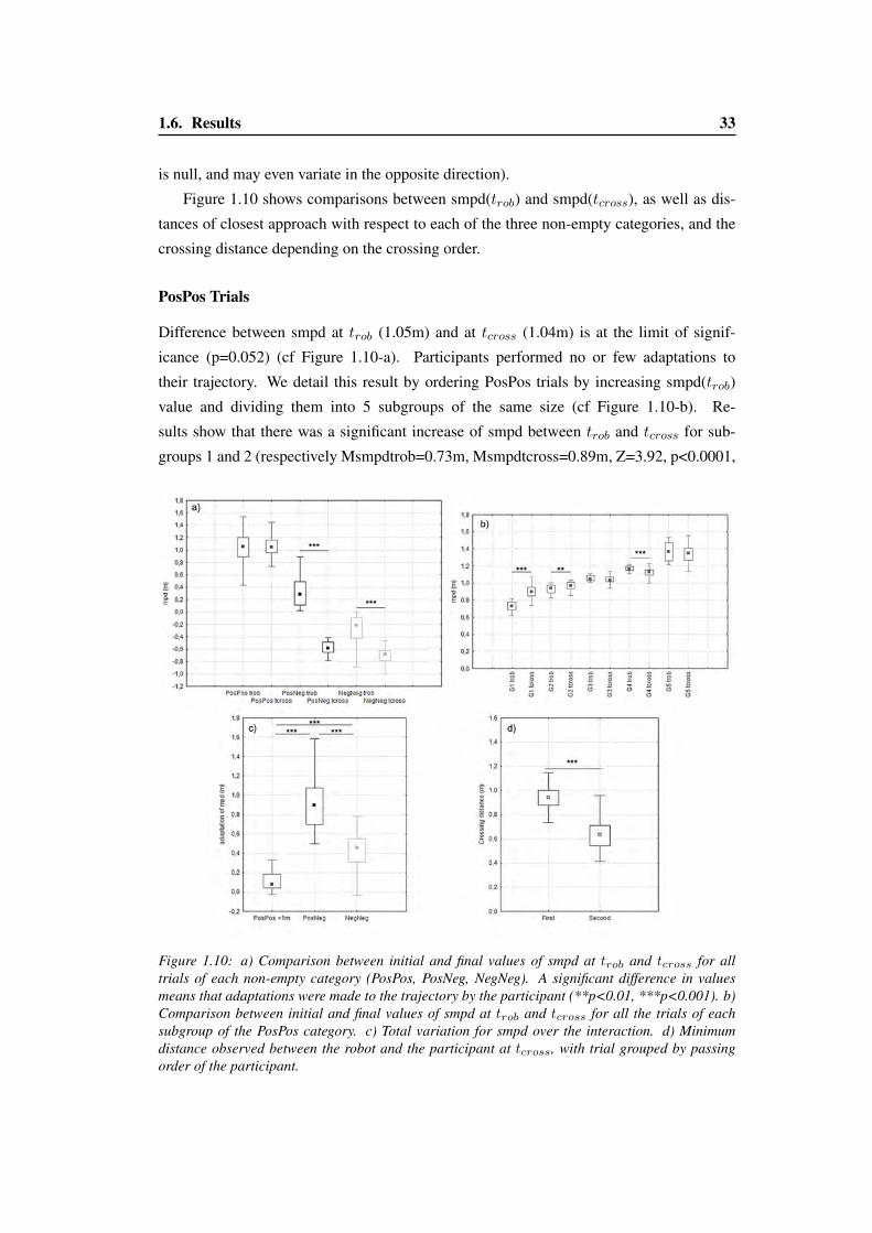
1.6. Results 33
is null, and may even variate in the opposite direction).
Figure 1.10 shows comparisons between smpd(trob) and smpd(tcross), as well as dis-
tances of closest approach with respect to each of the three non-empty categories, and the
crossing distance depending on the crossing order.
PosPos Trials
Difference between smpd at trob (1.05m) and at tcross (1.04m) is at the limit of signif-
icance (p=0.052) (cf Figure 1.10-a). Participants performed no or few adaptations to
their trajectory. We detail this result by ordering PosPos trials by increasing smpd(trob)
value and dividing them into 5 subgroups of the same size (cf Figure 1.10-b). Re-
sults show that there was a significant increase of smpd between trob and tcross for sub-
groups 1 and 2 (respectively Msmpdtrob=0.73m, Msmpdtcross=0.89m, Z=3.92, p<0.0001,
Figure 1.10: a) Comparison between initial and final values of smpd at trob and tcross for alltrials of each non-empty category (PosPos, PosNeg, NegNeg). A significant difference in valuesmeans that adaptations were made to the trajectory by the participant (**p<0.01, ***p<0.001). b)Comparison between initial and final values of smpd at trob and tcross for all the trials of eachsubgroup of the PosPos category. c) Total variation for smpd over the interaction. d) Minimumdistance observed between the robot and the participant at tcross, with trial grouped by passingorder of the participant.

34 Chapter 1. How humans avoid moving obstacle crossing their way?
r=0.88 and Msmpdtrob=0.94m, Msmpdtcross=0.97m, Z=3.17, p<0.01, r=0.71). For sub-
groups 3 and 5, there was no significant mpd variation between trob and tcross (respec-
tively Msmpdtrob=1.05m, Msmpdtcross=1.04m, p=0.14 and Msmpdtrob=1.37m, Msm-
pdtcross=1.35m, p=0.11). For subgroup 4 there was a significant decrease of smpd between
trob and tcross (Msmpdtrob=1.18m, Msmpdtcross=1.16m, Z=2.42, p<0.05, r=0.54). This
result suggests that when the initial value of smpd(trob) is lower than 1m, participants sig-
nificantly adapted their trajectory. Considering the previous example of PosPos trial in
Figure 1.6, we can confirm that the obtained results actually reflect the general behavior of
the participants. In addition, it was observed that when the pedestrian pass in front of the
obstacle, the distance between them is around 1 meter.
In the sequel we neglected subgroups 3, 4 and 5 since they do not capture avoidance
adaptations. The updated Pos-Pos group is then named PosPos<1m. Its median values of
smpd(trob) and smpd(tcross) were respectively 0.81m and 0.94m.
PosNeg Trials
Results show a significant difference of smpd between trob and tcross (Msmpdtrob=0.29m,
Msmpdtcross=-0.58m, Z=7.23, p<0.0001, r=0.86). When participants initially were likely
to pass first with an existing risk of collision, they finally decided to give way. Moreover,
it was observed that the distance between the obstacle and the walker at the crossing time
was around 0.5m.
NegNeg Trials
Results show a significant difference of smpd between trob and tcross (Msmpdtrob=-0.22m,
Msmpdtcross=-0.68m, Z=7.21, p<0.0001, r=0.87). When participants were likely to give
way, still with an existing risk of collision, they increased the future distance of closest
approach while maintaining the crossing order.
Quantity of adaptation
The more smpd variation, the more adaptation performed (Figure 1.10c). By Kruskal-
Wallis test, it results that there is an influence of the group on the quantity of adaptation:
H(2,180)=132.17, p<0.0001). Post hoc test showed that more adaptation are performed
for trials of the PosNeg group (M=0.90m) than for NegNeg (M=0.46m). Both show more
adaptation than for PosPos<1m (M=0.07mn), p<0.001.

1.7. Discussion 35
Crossing distance
The average distance of closest approach was 0.83m (± 0.27m). The crossing order influ-
enced this distance (Figure 1.10d). It was higher when participants passed first (M=0.94m)
(U=175, Z=-9.03, p<0.0001).
1.7 Discussion
We studied how humans adapt their trajectory to avoid collision with a moving robot.
We considered situations which are similar to previous studies on human-human collision
avoidance and our analysis was based on concept of smpd to enable comparisons.
Results show that, concerning some aspects, humans have similar behavior when avoid-
ing a robot or another human [Olivier 2012]. They accurately estimate the future risk of
collision: they do not perform adaptations when smpd is initially high (smpd(trob)>1m).
They also solve collision avoidance with anticipation. Figure 1.9 shows that smpd plateaus
in the latter period of interaction, called the regulation phase. A constant smpd indicates
that the avoidance maneuvers are over, and this happens significantly before tcross.
A significant difference about crossing configuration concerns the crossing order in-
versions that was observed in 29% of the trials: participants were initially likely to pass
first but adapted their trajectory to finally give way to the robot. This threshold can be
defined so that smpd(trob) is around 0.8m, which is the value of smpd(trob) for the Pos-
Pos<1m group: above this threshold, participants remain first, otherwise they change the
crossing order to give way to the robot. There was an overlapping in the smpd(trob) val-
ues between Pos-Pos<1m and Pos-Neg groups. To confirm such a threshold, we compared
these smpd(trob) values using a Mann-Whitney test. Results showed that smpd(trob) for
Pos-Pos<1m trials (M=0.81m) was higher than for the Pos-Neg trials (M=0.30m) (U=104,
Z=7.69, p<0.0001). We can link this 0.8m threshold to the crossing distance observed be-
tween two pedestrians in similar conditions [Olivier 2012] that was 0.81m. Moreover, it
was observed that when participants decide to pass in front of the robot, the distance at
the crossing time is around 1m while, in the case of PosNeg trials, such distance is around
0.5m. We correlated this difference to the concept of personal space and safer behavior.
The absence of inversion NegPos was also similarly observed and modeled by the
bearing angle theory [Kruse 2013]. Assuming that the robot obeys the bearing angle model
and the pedestrian contradicts it by re-inverting the sign of the bearing angle change, the
two adaptations could cancel each other out, ending into failure.
Which factors may explain such an inversion of role? We can assume that changing role
in the crossing order is somehow inefficient: no physiological or kinematic factor explains

36 Chapter 1. How humans avoid moving obstacle crossing their way?
this observation. It is not relevant to explain this based on perceptual factors (can humans
early perceive the role they are likely to have?). Indeed, inversion is observed in only one
direction (Pos-Neg), and we observed that the risk of collision is correctly perceived. We
interpret the role inversion as an extreme adaptation to preserve the personal space, directly
related to the perceived risk of collision. Passing in front of the robot may be perceived
as more dangerous. We suggest the following hypotheses to explain this feeling of danger.
First, humans ignored how the robot was controlled and its goal. The ongoing situation
cannot be easily predicted by pedestrians during short interactions. Even though we would
have instructed participants that the robot would not react to them, they may fear that the
robot would have unexpected motion changes. Our second hypothesis deals with the lack
of experience of participants to interact with an autonomous system. Humans perform
collision avoidance with other humans daily and they may expect collaboration from them.
Human-Robot collisions occur very rarely in real life. Our third hypothesis is about the
fear of getting hurt: visually the robot looks quite heavy, metallic and compact. Colliding
with it could certainly hurt legs which makes reasonable that participants prefer to adopt a
safer behavior than when crossing a human.
1.8 Conclusion
In the work described in this chapter, we reproduce the experimental protocol proposed by
Olivier et al. [Olivier 2013] in order to compare the differences between human-human
and human-robot collision avoidance. We programmed a moving robot to cross the path of
a walker in different ways: a) on a full collision course, b) on a partial collision course (the
robot was slightly in advance or late with respect to the participant), or c) not on a collision
course. In order to control the robot to obtain these configurations, the walking speed of
the participants was estimated once they reached their comfort speed. Results showed that
the strategies to avoid a moving obstacle have similarities with human-human interactions
(estimation of collision risk, anticipation) but also leads to some major differences. Hu-
mans preferentially give way to the robot, even though this choice is not optimal to avoid
collision. Moreover, humans never decided, in the cases in which they were second in the
crossing order, to accelerate and pass as first. We interpret this behavior based on the no-
tion of perceived danger and safety. This conservative strategy could be due to the lack of
understanding of how the robot behaves and the lack of experience of such an interaction
with an autonomous system. However, human always succeeded in avoiding the robot with
anticipation and without aberrant reaction. We also raised questions about humans reac-
tions facing a robot programmed to behave as a human. Would humans understand that the
robot cooperates and adapt their own strategy accordingly?
1.8. Conclusion 37
The conclusion of this study opens paths for future research. A first direction is to better
understand the possible effect of this notion of danger during human-robot interactions.
What are the aspects that influence more human perception (velocity, shape, size)? A
second direction is the design of safe robot motion amidst human walkers. How should the
robot adapt to humans? Should it be collaborative with the risk of compensating human
avoidance strategies? Should it be passive? We believe that robots should be first equipped
with human abilities to early detect human avoidance strategy and adapt to it.
In the next chapter, we will extend this study of human-robot crossing interaction: the
robot will be equipped with collision avoidance capabilities, imitating human strategies.
The idea is to investigate the differences on strategies set by participants if the robot is
cooperative instead of passive.


CHAPTER 2
Human and Robot interaction:cooperative strategies for collision
avoidance

2.1. Introduction 41
In the previous chapter we analyzed the human strategies to avoid an obstacle which
moves straight and at constant velocity. Tests showed that the participants preferred to give
way to the robot even if this solution was not optimal to avoid the obstacle. We hypothe-
sized that the lack of experience of the participants to interact with this kind of autonomous
systems implicate insecurity, and then they adopt a safer approach. In particular, we inter-
preted such a situation as a passive interaction: since the robot is not reacting but still mov-
ing, the participant could actually be surprised. Moreover, they adopt strategies that are
less performing with respect to the ones that they apply when they cross another human.
Therefore, our guess is that pedestrians would consider the robot as a non collaborative
agent or an unpredictable moving obstacle. This seems reasonable since humans are shar-
ing their environment daily with other humans, which lead them to develop implicit and
cooperative strategies based on the respect of social rules. Considering all these aspects,
in this chapter we present a new study in which the moving obstacle is now cooperative
and reactive in order to avoid the collision with the walker. The aim of this study is to
understand if the comfort1 of the pedestrian to share the environment with an autonomous
system can be improved if the robot behaves like a human.
2.1 Introduction
Since robots are progressively leaving their security cage to move in human popu-
lated environment, for applications such as service robotics or the factory of the fu-
ture, social aspects have to be considered to drive their behavior. Previous works
have shown that the compliance of the social aspects improve the acceptance, com-
fort and perceived safety of robots when they share the environment with other humans
[Buss 2011, Carton 2013, Lichtenthäler 2012]. Nowadays, social aspects are typically
taken into account to develop robot features inspired from humans [Breazeal 2005]. Read-
ability, legibility and predictability are terms widely used in this research area. In fact,
they describe the effect that it is easier for human to predict and understand the purpose of
motions if they are human-like [Carton 2013, Dragan 2013, Lichtenthäler 2013]. However,
it has not been defined yet whether human get used faster to interact with robots if they be-
have in a human-like way. Our work analyzes how humans react with a mobile robot that
behaves as a human. In particular, we focus on a collision avoidance task. Avoidance strate-
gies have been studied widely by psychologists, sociologists and in robotics. The general
goal is to avoid collision in accordance with a minimum effort principle and by preserving
the personal space. Several theories regarding the effectiveness of readable locomotion are
1In the sequel of this manuscript we will use the term "comfort" to indicate the natural behavior of a walker.In particular, "to improve the comfort" it means that the participant behaves smoother and more calmly.

42Chapter 2. Human and Robot interaction:
cooperative strategies for collision avoidance
provided in literature about the behavior of pedestrians. The sociologist Erving Goffman
observed in his studies that humans externalize themselves that means to make their desired
future motion predictable and clearer in a nonverbal way [Goffman 1971]. In his theory,
humans are consistently scanning the environment, especially the area in front of them,
when they walk towards and also expect others to act similarly. Moreover, pedestrians
scan the area mainly to perceive nonverbal signals from others to mutually avoid colli-
sions. Virtualization of avoidance behavior is widely studied in literature. Van Basten et al.
[van Basten 2009] synthesized human behavior for virtual characters in computer games
but without transferring rules about human-robot interactions. They based their work on
the concept of collaboration, anticipation, clearance and synchronization, by examining
the contribution of each agent to avoid collision. Reliastic collision avoidance for virtual
characters is also studied in [Karamouzas 2010]. One of the fundamental works in the hu-
man locomotion behavior has been provided by Fajen et al. [Fajen 2003]. They propose
a steering model to avoid collision at constant velocity, derived by human data. They also
compare the difference between the strategies set in real and in virtual environments. Ex-
periments in which two pedestrians are crossing each other (usually perpendicularly) are
considered by many studies [Albrecht 2012, Basili 2013, Huber 2014, Olivier 2013]. The
authors focus on personal behavior and respective adaptations. A specific common prin-
ciple is hard to find since several factors influence the results. Some approaches classified
velocity adaptation as the main strategies [Basili 2013] whereas others sustain that collision
avoidance is performed both in velocity and path adaptation (orientation) [Olivier 2012].
Recently, Carton et al. [Carton 2016] studies the differences between Human-Human and
Human-Robot moving face-to-face and the relative strategies to avoid collision. In order
to evaluate the effectiveness of readability for humans and robot, they compare the adapta-
tion in terms of path variation and velocity. Their experimental results show that readable
locomotion positively contribute to the locomotion planning of the other agent sharing the
same environment. Moreover, their study confirm that humans apply the same behaviors
for locomotion planning with humans and with robots. Human strategies to avoid a moving
obstacle that imitates a pedestrian behavior, in a real scenario and in a 90◦ crossing config-
uration has not still been considered. Our work moves forward in this direction. We repro-
duced the same experimental setup than previous studies ([Olivier 2013], [Vassallo 2017])
in order to understand the different reactions of a walker avoiding another human walker,
a passive moving obstacle and a cooperative robot. Comparisons are based on the concept
of smpd introduced in the previous chapter.
The chapter is structured as follows. The experimental setup and the apparatus are
explained in Section 2.2. In particular, we highlight the improvements made in this context,
in order to improve the quality of the results. The way how we control the robot to behave

2.2. Materials and Methods 43
as human is presented in Section 2.3. Follows the relative analysis based on smpd and then
the discussion. We also compared the avoidance strategies when the robot is active with
respect to the passive one previously studied. A conclusive section ends the chapter.
2.2 Materials and Methods
2.2.1 Participants
Ten volunteers participated in the experiment (2 women and 8 men). They were 29.2
(± 8.4) years old and 1.74m tall (±0.11m). They had no known vestibular, neurological or
muscular pathology that would affect their locomotion. All of them had normal or corrected
sight and hearing. Participants gave written and informed consent before their inclusion in
the study. The experiments respect the standards of the Declaration of Helsinki (rev. 2013),
with formal approval of the ethics evaluation committee Comitè d’Evaluation Ethique de
l’Inserm (IRB00003888, Opinion number 13-124) of the Institut National de la Santé et de
la Recherche Médicale, INSERM, Paris, France (IORG0003254, FWA00005831). All the
participants were equipped with 6 markers fixed to a helmet that they were wearing.
2.2.2 Apparatus
The experimental setup was almost identical to the one already presented in Section 1.3.
The experiments took place in 50m x 25m gymnasium. Two areas were defined and sep-
arated by 2m high occluding walls, forming a gate in the middle. One of the problems
of the previous experiment was that the lateral area of the gymnasium was not sufficiently
covered by the cameras field of view. To this end, the devices were reorganized such that
the robot starting position could be farther (around 2 meters more for each side). Thereby,
the accuracy of the tracking was improved since the starting position of the real robot and
the virtual one was almost the same or really near. An overview of the experimental setup
is shown in Figure 2.1. Four specific positions were identified: the participant starting po-
sition PSP, the participant target position PT, and two robot starting positions RSP1 and
RSP2. The walking speed was measured in the Motion Estimation Zone area (MEZ). With
respect to the previous chapter, the participant were starting to move from farther, in the
uncovered area. We improved the system in order to identify and track the actor position
in a faster way. To this end, the distance between PT and MEZ was increased from 1.6m to
4m, allowing participants to reach their cruise speed more comfortably. The length of the
MEZ area was extended too, from 2.8m to 3.5m. The intersection point of the robot path
[RSP1, RSP2] and the participant path [PSP, PT] is named Hypothetical Crossing Point
HCP. In this experimental setup we added two new positions next to HCP: the via points

44Chapter 2. Human and Robot interaction:
cooperative strategies for collision avoidance
PSPMotion Estimation
Zone
PT
RSP1
RSP2
HCP gate
4m3.2m2.8m3.2m
1.4
m
occluding divider screen
1m 0.5m
t_see
0.67m
Figure 2.1: Experimental apparatus and task. The covered area was extended with respect to theprevious work.
VP1 and VP2. They are defined as intermediate waypoints in the robot trajectory to pass
behind or in front of the participant (more details in Section 2.3.2).
2.2.3 Participant Task
Participants were asked to walk at their preferred speed from PSP to PT by passing through
the gate. They were told that an obstacle will be moving over the gate and could interfere
with them. Participants were completely unaware about the robot behavior. One experi-
mental trial corresponds to one travel from PSP to PT.
2.2.4 Recorded Data
3D kinematic data were recorded using the motion capture Vicon-MX system (100Hz).
Reconstruction was performed using Vicon-Blade and computations using Matlab (Math-
works r). The experimental area was covered by 15 infrared cameras. Contrary to pre-
vious experiments, we estimated the global position of participants as the centroid of re-
flective markers set on the helmet that they were wearing, because it was less subjected
to noise, especially during the crossing through the door. The stepping oscillations were
filtered out by applying a Butterworth low-pass filter (2nd order, dual pass, 0.5Hz cut-off
frequency).

2.3. Robot Behavior 45
ID Trial Cooperative Behavior RSP Side SMPD ID Trial Cooperative Behavior RSP Side SMPD1 Yes Left -0.6 31 No Left 02 Yes Right 0 32 Yes Right 0.33 Yes Right 0.6 33 No Left 0.64 No Right -0.9 34 Yes Left 0.95 Yes Left -0.3 35 No Right – –6 No Right 0.9 36 No Left -0.37 Yes Left -0.3 37 Yes Left -0.98 No Right 0.6 38 No Left 0.99 No Right -0.6 39 Yes Left 0.6
10 Yes Right 0.9 40 Yes Right 0.911 No Right -0.9 41 Yes Left 012 Yes Left 0.3 42 Yes Right -0.613 Yes Left 0 43 Yes Left -0.914 No Right 0.3 44 No Right 015 Yes Right 0.6 45 No Right -0.316 No Right – – 46 No Left -0.617 Yes Right -0.3 47 Yes Left 0.318 Yes Right 0.3 48 No Left 0.619 No Right -0.3 49 Yes Right 020 No Left 0.9 50 No Right 0.921 No Left – – 51 Yes Right -0.622 Yes Left 0.9 52 Yes Right -0.323 No Left 0.3 53 No Left -0.324 No Right 0.6 54 No Left – –25 No Right 0 55 No Left -0.626 No Left 0 56 No Left 0.327 No Right 0.3 57 Yes R -0.928 Yes Right -0.9 58 Yes Left -0.629 Yes Left 0.6 59 No Left -0.930 No Left -0.9 60 No Right -0.6
Table 2.1: Organization of the trials
2.2.5 Experimental plan
Each participant performed 60 trials (see Table 2.1). The robot starting position (50% in
RSP1, 50% in RSP2) was randomized among the trials. To introduce a bit of variability,
in 4 trials the robot did not move and so the participant did not have to react. Only the 56
trials with potential interaction were analyzed.
2.3 Robot Behavior
We used a prototype of RobuLAB10 wheeled robot from the Robosoft company (dimen-
sion: 0.45 x 0.40 x 1.42m, weight 25 Kg, maximal speed around 3 m/s) (see Figure 1.2b).
The robot position was detected as the center point in its base. Despite previous work, we
limited the smpd trials in the range [-0.9m, 0.9m] since it was observed that over this range

46Chapter 2. Human and Robot interaction:
cooperative strategies for collision avoidance
the interactions were not significant. We control the robot to behave either cooperatively
or passive (50% passive and 50% active). In the cases in which the robot was active, in
function of smpd sign, it decided to move in such a way to maintain its role (even if this
choice was not optimal). The two behaviors were randomized among the trials.
2.3.1 Passive Behavior
In this work we also replicated the robot passive behavior in order to confirm the previ-
ous results and compare them with the new ones. The robot was controlled to generate
specific interactions with the participant; the robot was either: a) on a full collision course
(reach HCP at the same time than the participant), b) on a partial collision course (the robot
reaches HCP slightly before or after the participant), or c) not on a collision course. Walk-
ing speed was measured in MEZ and the crossing configuration was computed as a function
of the desired smpd, exactly as in the previous work. Each trial was repeated twice.
2.3.2 Cooperative Behavior
In the previous chapter, we observed that humans behave differently depending on whether
they have to pass in front of the obstacle or behind. In particular, it emerged that if they pass
ahead the obstacle, the distance is greater than when passing behind. In fact, the distance
are respectively around 1m and 0.5m. Moreover, participants were used to accelerate to
pass as first or decelerate to give way. Based on these observations, in the new experiments
the robot is controlled in order to behave as a human. Initially its velocity is regulated to
be equal to the one of the participant.
Once the interaction phase begins (the walker had almost crossed the door and the robot is
visible at tsee) (see Figure 2.2), we generate specific reactive movements of the robot based
on the value of smpd:
- when robot is late (smpd > 0): the vehicle is controlled to first decelerate and then
turn to pass behind the human, see Figure 2.2, 2.3(a);
- when the human is late (smpd < 0): the vehicle is controlled to first accelerate and
then turn to pass in front of the human, see Figure 2.3(b), 2.3(c);
- in case of full collision course (smpd = 0): given the actor position and the relative
velocity, the robot estimates at tsee who is reaching HCP as first. Then it reacts to
pass as first or to give way, as in the cases of smpd<0 or smpd>0 respectively.
At the beginning of each trial, the software read the relative trial configuration (Ta-
ble 2.1). The robot starting position was computed in real time, based on the actor velocity.
Once the actor was over the MEZ area, the robot started to move at the same speed as the

2.4. Analysis 47
pedestrian. We estimate this velocity as in the previous study (Kalman Filter, material point
moving along a line, no acceleration).
2.4 Analysis
2.4.1 Kinematic data
The analysis of the data for the trials in which the robot as a passive behavior was the
same as in the previous chapter. We computed trob, the time at which the robot reaches
its constant cruise speed (acceleration below a fixed threshold, 0.003 m/s2), and tcross,
the time of closest approach between the participant and the robot. However, for the trials
in which the robot is active, we cannot define trob since the reactive behavior of the robot
implies several variations of its velocity. Moreover, in the previous chapter, we considered
trob instead of tsee because the aim of the work was to analyze the human strategies to
avoid a passive obstacle. The smpd components relative to the robot were minimized and
the participants mainly contributed to change the smpd. However, in the following work,
PSPMotion Estimation
Zone
PT
RSP1
RSP2
4m3.2m2.8m3.2m
1.4
m
occluding divider screen
1m 0.5m
VP1
HCP
gate
t_see
0.67m
Figure 2.2: Experimental setup when robot is cooperative. The pedestrian moves from PSP to thegate through the MEZ. At 0.67m before crossing the gate, the actor is able to see the robot (tsee).In the following trial, the robot decelerates and passes behind the actor, going through VP1. Thered robot and the red actor illustrate the hypothetical crossing configuration.

48Chapter 2. Human and Robot interaction:
cooperative strategies for collision avoidance
PT
RSP1
3.2m
VP1
gate
t_see
0.67m
(a)
PT
RSP1
3.2m
VP2
gate
t_see
0.67m
(b)
PT
3.2m
VP2
RSP2
1m 0.5m
gate
t_see
0.67m
(c)
Figure 2.3: (a) smpd>0: The robot starts from RPS1, decelerates and turns right. (b) smpd<0:the robot starts from RPS1, accelerates and turns left. (b) smpd<0: the robot starts from RPS2,accelerates and turns right.

2.5. Results 49
we control the robot to be either passive or active. Therefore, when the robot is active,
the smpd is influenced both by the robot and the participant. So that, we consider the
interaction phase starting at tsee, the time in which the participant was approaching the
gate. The general profile of the smpd was tested with different distances from the door,
from which we supposed that the person could start seeing the robot. In particular we
compare the general behavior when the participant was before, exactly and slightly over the
door line. Tests showed that reliable results are obtained if we consider tsee as the instant
of time where the participant passed the door of 0.2 meter. This is due to the high variation
of the mobile robot velocity at its start. Similarly to the previous chapter (see page 33) four
different groups of trials were considered, according to the sign of mpd at the beginning
and at the end of the interaction: PosPos, PosNeg, NegPos and NegNeg. We considered
trob for the trials in which the robot is passive and tsee for the ones in which it is active.
2.4.2 Statistics
All the statistical analyzes were performed using Statistica (Statsoft r). All effects were
reported at p<0.05. We normalized all the data by using a Kolmogorov-Smirnov test. Based
on the normality, the values are expressed as median (M) or mean ±SD. The variation of
smpd sign during the interaction time was determined by Wilcoxon signed-rank tests. To
compare the crossing distance depending on the final crossing order, we used a Mann-
Whitney test.
2.5 Results
We considered 552 trials because 8 of the 560 initial trials were removed, as the robot failed
to start. Each participant performed 60 trials of which 4 were not considered because the
robot did not move and so there was no interaction. In each experience, the robot was
active for 50% of the trials and passive for the remaining 50%. In total, we had 274 trials
where the robot was active and 278 where it was passive. The analysis and the results
have been divided for the two cases. At the end of the chapter, based on the behavior of
the participants, these two cases will be compared with each other. Statistical results were
computed considering 280 trials.
2.5.1 Passive Robot
We based our analysis on the concept of smpd. In particular, we investigated the smpd
values at trob and tcross. It resulted that, at the beginning of the interaction, the participants
were first in the crossing order in 38.41% of all cases. However, they decided to give way

50Chapter 2. Human and Robot interaction:
cooperative strategies for collision avoidance
in 15.22% of trials. Globally, it emerges that the smpd categories are distributed among
the trials in the following way: PosPos=64 trials (23.18%), NegNeg=169 trials (61.23%),
PosNeg=42 trials (15.22%), NegPos=1 trial (0.36%). Clearly, this last category won’t be
considered in the future analysis. The evolution of the smpd for all the trials is depicted in
Figure 2.4.
Comparing these results with the one of the previous chapter (Figure 1.9, page 32), it
emerges that the general behavior is almost identical. Examples of corresponding trajec-
tories are illustrated in Figure 2.5. The mean evolution of the smpd for each category is
shown in Figure 2.6.
Statistical Results
Since we reduced the smpd range (from [-1.2m,1.2m] to [-0.9m,0.9m]) we did not observe
too many trails in which there is no interaction for PosPos and NegNeg groups. For this
reason, we did not subdivided these two groups into subgroups for further analysis. From
the statistical analysis of the variation of the smpd between trob and tcross , it results that
participants performed significant adaptations in all the groups.
Table 2.2 shows the median value of smpd at trob, Msmpdtrob, and at trob, Msmpdtcross.
0 10 20 30 40 50 60 70 80 90 100
−2
−1.5
−1
−0.5
0
0.5
1
1.5
2
2.5MPD Normalized Signed (Passive)
MP
D [m
]
Time Normalized
Figure 2.4: smpd plots for all the 278 trials, after resampling over the interaction time [trob, tcross].

2.5. Results 51
From Statistica, we report the Wilcoxon signed-rank test using the Z parameter (r repre-
sents the reliability of the test). The reader is invited to give a look at Figure 2.6 to better
understand the results described below.
Table 2.2: Statistical analysis results of the smpd data during trob and tcross in the case that therobot is passive. The Wilcoxon signed-rank test was performed using Statistica v.8 .
Category Msmpdtrob Msmpdtcross Z rPosPos 0.73m 1.05m 4.04 0.7379PosNeg 0.41m -0.83m 5.23 0.8719NegNeg -0.58m -0.84m 4.69 0.5739
PosPos Trials
Results show a significant difference of smpd between trob and tcross and they confirm the
ones presented in the previous chapter. Participants adapted their trajectory to pass first if
the smpd(trob) was less than 1 meter, otherwise no adaptation was noticed.
Figure 2.5: Examples of participant and robot trajectories for each category of trial. The boldtrajectory represents the interaction time [trob, tcross].

52Chapter 2. Human and Robot interaction:
cooperative strategies for collision avoidance
0 10 20 30 40 50 60 70 80 90 100
−1.5
−1
−0.5
0
0.5
1
1.5
Mean MPD Passive
Mea
n M
PD
[m]
Time Normalized
PosPosPosNegNegPosNegNeg
(a) Mean evolution of smpd for each category of trial.
0 10 20 30 40 50 60 70 80 90 100
−1.5
−1
−0.5
0
0.5
1
1.5
2Mean MPD POSPOS Passive
Mea
n M
PD
[m]
Time Normalized
(b) PosPos
0 10 20 30 40 50 60 70 80 90 100
−1.5
−1
−0.5
0
0.5
1
1.5
2Mean MPD POSNEG Passive
Mea
n M
PD
[m]
Time Normalized
(c) PosNeg
0 10 20 30 40 50 60 70 80 90 100
−1.5
−1
−0.5
0
0.5
1
1.5
2Mean MPD NEGNEG Passive
Mea
n M
PD
[m]
Time Normalized
(d) NegNeg
Figure 2.6: Mean evolution of smpd±1 Standard Deviation for the three categories where the robotis passive.

2.5. Results 53
PosNeg Trials
Results show a significant difference of smpd between trob and tcross and they confirm the
ones presented in the previous chapter. When participants initially were likely to pass first
with a possible risk of collision, they decided to give way to the robot. Such a behavior is
observed if there exists an high risk of collision (future crossing distance around 0.5 meter).
NegNeg Trials
Results show a significant difference of smpd between trob and tcross and they confirm
the ones presented in the previous chapter. Participants maintained the crossing order by
giving way to the robot. If the future crossing distance was small enough to be considered
as risky, participants also adapted their trajectory to increment it.
2.5.2 Cooperative Robot
As previously explained, we consider tsee as the instant of time at which the reaction phase
begins. The sign of mpd at tsee shows that the participant passed first in 52% of all cases
and gave way in the other 48%. Combining this information with the sign of mpd at tcross,
it turns on that the smpd categories are distributed among the trials in the following way:
PosPos=140 trials (50.91%), NegNeg=110 trials (40%), PosNeg=22 trials (8%), NegPos=3
trials (1.09%). The evolution of the smpd for all the trials is depicted in Figure 2.7. Since
NegPos group is composed by only 3 trails that are mainly outliers, we will not consider
them in the future analysis.
If we compare these results with the ones observed in the previous chapter (Figure 2.4,
page 50), it appears that the general behavior is slightly changed. In fact, we still have Pos-
Neg trials but the crossing order is mainly preserved. Such preservation of the roles reflects
more the behavior observed by Olivier et al. [Olivier 2013] with two humans crossing each
other. The mean evolution of the smpd for each category is shown in Figure 2.8. Examples
of corresponding trajectories are illustrated in Figure 2.9.

54Chapter 2. Human and Robot interaction:
cooperative strategies for collision avoidance
Figure 2.7: smpd plots for all the 278 trials, after resampling over the interaction time [tsee, tcross].
Statistical Results
In the experiments with a cooperative robot, the average behavior of the smpd for all the
categories is more uniformly distributed among all the trials. In particular, we notice that
the switch of roles PosNeg is more sporadic (only 8% of trials). We statistically analyzed
the smpd at tsee and tcross in order to understand if there is a significant variation: partici-
pants performed considerable adaptations in all the groups. Results are shown in Table 2.3,
where Msmpdsee and Msmpdtcross are respectively the medium value of smpd at tseeand tcross. Also in this case, the reader is invited to give a look at Figure 2.8 to better
understand the following results.
Category Msmpdtsee Msmpdtcross Z rPosPos 0.71m 1.08m 9.17 0.7863PosNeg 0.29m -0.71m 8.98 0.8748NegNeg -0.46m -1.14m 4.11 0.8711
Table 2.3: Statistical analysis results of the smpd data during tsee and tcross in the case that therobot is passive. The Wilcoxon signed-rank test was performed using Statistica v.8 .

2.5. Results 55
0 10 20 30 40 50 60 70 80 90 100
−1.5
−1
−0.5
0
0.5
1
1.5
Mean MPD Active
Mea
n M
PD
[m]
Time Normalized
PosPosPosNegNegPosNegNeg
(a) Mean evolution of smpd for each category of trial.
0 10 20 30 40 50 60 70 80 90 100
−1.5
−1
−0.5
0
0.5
1
1.5
2Mean MPD POSPOS Active
Mea
n M
PD
[m]
Time Normalized
(b) PosPos
0 10 20 30 40 50 60 70 80 90 100
−1.5
−1
−0.5
0
0.5
1
1.5
2Mean MPD POSNEG Active
Mea
n M
PD
[m]
Time Normalized
(c) PosNeg
0 10 20 30 40 50 60 70 80 90 100
−1.5
−1
−0.5
0
0.5
1
1.5
2Mean MPD NEGNEG Active
Mea
n M
PD
[m]
Time Normalized
(d) NegNeg
Figure 2.8: Mean evolution of smpd±1 the Standard Deviation (SD) for the three categories wherethe robot is cooperative. The category NegPos was not considered.

56Chapter 2. Human and Robot interaction:
cooperative strategies for collision avoidance
Figure 2.9: Examples of participant and robot trajectories for each category of trial. The boldtrajectory represents the interaction time [tsee, tcross].
PosPos Trials
Results show a significant difference of smpd between tsee and tcross. Participants pre-
served the crossing order if the smpd(tsee) was around 0.65m. In contrast to the previous
results, the average behavior is shifted toward the zero of around 0.2m. It means that, even
if the risk of collision was high (0.1m), there was no an arbitrary switch of roles.
PosNeg Trials
Results show a significant difference of smpd between tsee and tcross. Similarly to the
previous experiments, the participant decided to give way to the robot if significant risk of
collision existed (future distance around 0.35m). However the PosNeg trials are few with
respect to the experiments where the robot was behaving passively (8% versus 15.21%).

2.6. Discussion 57
NegNeg Trials
Results show a significant difference of smpd between tsee and tcross. During NegNeg
trials, both the actor and the robot were positively contributing to maintain the crossing
order. Indeed, by comparing Figure 2.8(d) and Figure 2.6(d) it can be noticed that there
is an increment of smpd. This variation is bigger than for the PosPos group, because the
actors behaved in order to maintain a larger distance from the robot, compared with the case
in which they pass behind. This results is coherent with the one observed in the previous
experiments: participants passed closer to the robot closer when passed behind.
2.5.3 Crossing Distance
The average distance of closest approach for PosPos and NegNeg group is 1.13m (± 0.3m).
It is 1.10m (± 0.31m) for the PosNeg group.
2.6 Discussion
We investigated the strategies set by humans to avoid a moving robot. We considered
a situation similar to the one of previous studies on collision avoidance between two
humans [Olivier 2013] and collision avoidance between a human and a robot moving
straight at constant speed (Chapter 1). The analysis was based on smpd (Section 1.5) to
enable comparison. We programmed the robot to be either passive or cooperative. In the
first case, we confirmed the previous results: participants do not perform adaptation if
the smpd is initially high (smpd(trob>1m) and the collision avoidance is performed with
anticipation. Moreover, participants preferred to give way to the robot although they were
likely to pass first. It results that in most of the cases (76.45%), the participants pass
second. Considering the trials in which the robot was active, we observed similarities but
major differences. Similarly to human-human interaction, the crossing order is mainly
respected (around 90% of all cases). However, we still observe a tendency of actors to give
way to the robot (PosNeg group corresponds to 8% of trails). The switch of roles NegPos
was not observed.
Which factors may explain such a change of behavior between passive and cooperative
cases? It appears that the inactive behavior of the robot is somehow counterproductive.
Humans daily set implicit strategies when they have to cross each other. When pedestrians
have to interact with an autonomous system, the feeling of insecurity and danger may be
natural because they are not used to share their environment with robots. In the previous
discussion, we hypothesized that participants preferred to preserve their personal space

58Chapter 2. Human and Robot interaction:
cooperative strategies for collision avoidance
rather than succeeding the collision avoidance task quickly and smoothly. However, in
view of the last results, it appears that when the robot applies the observed human avoidance
strategies, the comfort of the pedestrians is eased. Considering the number of trials in which
the crossing order is preserved, we clearly observed that the robot behavior successfully
suggests the future crossing order to the human. In the previous work [Olivier 2013], our
partners found out that the participant giving way (#2) was contributing more than the one
passing first (#1). Moreover, it resulted that the participant #2 preferred to adapt mainly
his speed during at the beginning of the interaction and, in turn, both participants were
adapting their orientation. This behavior was similarly observed in the last experiments:
the robot was initially accelerating or decelerating and then it slightly turned. Although
such a behavior was not really evident, it was sufficient for the pedestrians to understand
the intentions of the robot and then, in turn, their own role on the crossing order.
2.7 Conclusion
In this chapter, we used the experimental protocol proposed by Olivier et al. [Olivier 2013]
and Vassallo et al. [Vassallo 2017]. We based our analysis on the concept of smpd intro-
duced in Section 1.5. In these last experiments we programmed a wheeled robot to move
either passively (as well as in the previous chapter) or in a cooperative way. In order to be
cooperative, the robot follows simplified observed strategies that were identified in humans:
it accelerates and turns to pass ahead the participant or it decelerates and turns to pass be-
hind. Since the study of this work is divided in two parts, we obtained several results that
could have compared. Firstly, we confirm the observations previously presented: humans
do not behave optimally in terms of time and energy when they have to interact with a pas-
sive robot. They prefer to preserve their personal space. Secondly, we observe how humans
react if the robot cooperates to avoid the collision. Results show that walkers behave more
naturally: the crossing order is respected in most of cases and the adaptations, in terms of
speed variation, are smoother. Although we observed a change of roles (8% of cases), we
related this phenomenon to the fact that pedestrians have still a tendency to give way to the
robot. We hypothesize that, with appropriate analysis and improvements of the observed
strategies, the percentage of change of roles could be further decreased. Therefore we con-
clude that, in terms of safety and efficiency, the performance of human-robot collaboration
is improved if the robot behaves in a human-like way. This result was already observed in
literature by many authors [Kato 2015, Dragan 2015]. In addition, we proved the verac-
ity of the hypothesis, proposed by [Carton 2013, Dragan 2013, Lichtenthäler 2013]: it is
easier for humans to predict and understand the purpose of the robot motions if they are
human-like.

CHAPTER 3
Learning Movement Primitivesfor the Humanoid Robot HRP2


3.1. Introduction 61
The modeling of online reactive motion is an important challenge in humanoid robotics.
In particular, the generation of complex full-body movement, maintaining the dynamic
stability of the gait, is an extreme difficult task, although it is a natural behavior for humans.
Therefore, walking pattern generators have to consider online-reactive motion of both low-
body and upper-body part. The work presented in this chapter provides a new step in
this direction. It has been done in collaboration with computational neuroscientists of the
University Clinic Tubingen, within the framework of the European project Koroibot. We
propose a new approach to synthesize realistic complex humanoid robot movements with
motion primitives. The control framework proposed combines biologically-inspired online
planning for the upper body and model predictive control for the lower body. The upper-
body movements are generated via a coupled dynamical motion primitives. Such primitives
are learned from human data recorded with a motion capture system, after appropriate re-
targeting and adjustment in order to respect the constraints of the robot. The lower body
is controlled by the walking pattern generator developed al LAAS-CNRS by Naveau et al.
[Naveau 2017].
3.1 Introduction
The planning of flexible and adaptive behavior for humanoid robots cannot be accom-
plished satisfactorily by the off-line synthesis of dynamically stable behaviors. The rea-
son for that is the continuous change of the environment and the error in state estimations.
Moreover, the optimal control of human-like multi-joint systems is a computationally chal-
lenging problem. Current solutions involve near real-time whole body Model Predictive
Control with regularized modeling of contacts in order to decrease the associated computa-
tional cost [Tassa 2012, Koenemann 2015]. A precise modeling of contact phases requires
hours of offline computation time [Koschorreck 2012]. Another challenging issue for the
generation of human-like behaviors is the sequential planning of multi-step sequences,
where individual steps can be associated with different sub-goals or constraints (like con-
tact with goal objects or step-length constraints). This problem being multidisciplinary,
we quickly review associated work in computer graphics, biological motor control, and
humanoid robotics.
3.1.1 Modeling of whole-body movements in computer graphics
Synthesizing complex whole body movements is a problem widely addressed in com-
puter graphics, e.g. [Levine 2012], and many learning-based approaches have been pro-
posed that provide low-dimensional parametrization of classes of whole body motion

62Chapter 3. Learning Movement Primitives
for the Humanoid Robot HRP2
[Hsu 2005, Wang 2008]. In particular, recent works focused on methods for the blend-
ing of learned motion primitives, whose concatenations over time have to satisfy additional
task constraints. For example, in [Feng 2012] captured motion samples were blended ex-
ploiting a "prioritized stack of controllers". In [Shoulson 2014] the instantaneous blending
weights of controllers were prioritized by their serial order. In [Huang 2014] the coordina-
tion between locomotion and arm pointing in the last step was modeled by blending and
selecting arm pointing primitives dependent on the gait phase.
3.1.2 Biological motor control of multi-step sequences
Human motor behavior including action sequences has been shown to be highly predictive.
This has been investigated, for example, in a recent study on the coordination of walking
and reaching [Land 2013]. Human subjects had to walk towards a drawer and to grasp an
object, which was located at different positions in the drawer. Participants optimized their
behavioral from multiple steps before the object contact, predicting the maximum end-state
comfort during the reaching action [Weigelt 2010, Rosenbaum 2008]. This means that the
steps prior to the reaching were modulated in a way that optimizes the distance for the
reaching action [Land 2013]. In [Mukovskiy 2015a], our KoroiBot partners have proposed
a learning-based framework that is based on movement primitives, learned from motion
capture data. They are able to reproduce such human planning strategies in computer ani-
mation. The underlying architecture is simple and approximates complex full-body move-
ments by dynamic movement primitives that are modeled by nonlinear dynamical systems.
These primitives are constructed from kinematic primitives that are learned from trajectory
sets by an anechoic demixing. Similarly to previous works [Gams 2008, Buchli 2006],
the proposed method generates complex movements by combination of a small number
of learned dynamical movement primitives. [Mukovskiy 2015a, Giese 2009a] have previ-
ously demonstrated the advantages of this approach for the adaptive online generation of
multi-step sequences with coordinated arm movements.
3.1.3 Related approaches in humanoid robotics
Several approaches have been proposed in robotics for the synthesis of walking combined
with grasping movements. Indeed, the DARPA robotics challenge valve manipulation task
forced the researchers to find efficient and robust methods to perform reaching and ma-
nipulation tasks. [Ajoudani 2014] proposed a hybrid controller, where the robot is using
a goal-driven fast foot step planner in combination with visual servoing for the reaching
and grasp of the valve. [Kuindersma 2015] proposed a complete control architecture for
the humanoid robot Atlas that is able to localize the robot and automatically find foot steps

3.1. Introduction 63
around or over obstacles in order to reach a user-defined goal. The architecture contains
also a whole-body controller which allows the robot to get up from a lying down position, or
to do complex tasks like turning the valve. Another team (IHMC) presented an architecture
in [Johnson 2015] with a more sophisticated control of the locomotion [Englsberger 2014].
All three mentioned control architectures can make a humanoid robot reach, and then grasp
or manipulate objects as required for the robotics challenge. Walking to grasp and manip-
ulation tasks are usually subdivided in two different sub-tasks and, to our knowledge, a
simultaneous coordination of both tasks has not been demonstrated so far. Other solu-
tions for the combination of walking and vision-controlled reaching of a static and mo-
bile target during walking were proposed in [Stasse 2008] and [Brandao 2013]. Other ap-
proaches include adaptation of randomized motion planning algorithms to generate com-
plex body motion in a constrained environment [Dalibard 2013], but with the disadvantage
of high computational time. A further work based on imitation and learning has been pro-
posed by [Miihlig 2010], which also combines walking and grasping as two separate tasks.
[Gienger 2010] proposed an algorithm for the computation of optimal stance locations with
respect to the position of a reaching target, where a dynamical systems approach was used
to generate the reaching behavior. [Yoshida 2007] used a task priority approach, based on
a generalized inverse kinematics, in order to organize several sub-tasks, including step-
ping, hand motion, and gaze control. Another work has exploited global path planning in
combination with walking pattern generators (WPGs) [Kajita 2003], in order to generate
collision-free dynamically stable gait paths. A first attempt to transfer human reaching
movements to humanoid robots by using motion-primitives was proposed in [Taïx 2013].
In this work the primitives were extracted by using PCA and the behavior was success-
fully implemented on the HRP-2 robot by involving the trunk and arm joints. The use of
motion primitives in robotics was also proposed in [Gams 2013], which even includes the
integration of force-feedback. Systems which are able to modulate dynamical movement
primitives to generate complex motion in real-time were proposed by [Ijspeert 2013] and
[Ajallooeian 2013].

64Chapter 3. Learning Movement Primitives
for the Humanoid Robot HRP2
3.2 System architecture
In this section the whole process that we used to generate walking to grasp motion is il-
lustrated, starting from the recorded human data. The acquisition of data through motion
capture, the scaling and the adaptation to match the humanoid robot constraints, the rel-
ative decomposition in dynamic primitives and the learning part have been developed by
our Koroibot partner from Tübingen [Mukovskiy 2015b]. Our principal contribution was
to implement the unstable trajectories inside the walking pattern generator (developed at
LAAS-CNRS by Naveau et al. [Naveau 2017]) and to combine the two sub-tasks (grasping
and walking) into a single one which is feasible and dynamically stable.
A general overview of the system architecture is shown in Figure 3.1. The extraction of
the training data from the human data and the relative segmentation and re-targeting have
been done offline. However, the generation of movement by the learned re-targeted motion
primitives and the robot control have been performed online.
3.2.1 Human data
3.2.1.1 Drawer opening task
The modeling of walking-to-grasp was based on a motion capture data set obtained by
recording humans walking toward a drawer and grasping an object. In the experiment, the
initial distance from the drawer and the position of the object inside it was varied, in order
to analyze the adapting behavior [Mukovskiy 2015a] (see Figure 3.2 and a related video1
available online). The whole motion can be sub-divided in three parts:
1. normal walking, starting and ending with the left heel strike,
2. adaptive stepping until reaching the drawer with the left hand,
3. grasping, end of walking and taking the object with the right hand.
Figure 3.1: General overview of the system architecture.

3.2. System architecture 65
The data set consists of the trajectories of ten trials of a single participant performing the
task. The human data was recorded at Bielefeld University with a Vicon motion capture
system, consisting of 12 MX-F20 CCD cameras (f=400Hz, accuracy of 1.5mm). The actor
was equipped with 41 markers. The length of each action, in terms of space, is shown in
Figure 3.3(a).
3.2.1.2 Preprocessing
The recorded motion capture was processed and animated with the 3D Character Ani-
mation Software MotionBuilder (Autodesk), using an avatar whose geometric parameters
were adapted to the recorded subject. The trajectory were cut, starting at the first heel strike
and ending once the object was reached. The kinematic model of HRP was created with
the Computer Animation and Modeling Software Maya (Autodesk), neglecting kinematic
constraints. All the ten trajectories were re-targeted to the HRP-2 model in MotionBuilder.
In particular, the markers were fixed on the avatar body, scaled and synchronized, in order
to "control" the virtual character motion by the recorded real trajectories. In other words,
the avatar was "moved" by the real markers, reproducing the human motion. During re-
targeting, the feet position was constrained to be parallel to the level ground. Also the step
lengths were scaled in order to match the size difference between the actor and HRP-2.
Once obtained the resulting scaled motion with the virtual character, the joint trajectories
were extracted using the Denavit-Hartenberg (DH) convention. In turn, they were seg-
mented and the step sizes were stored separately. The computed trajectories were further
analyzed with Matlab (Mathworks r) and re-sampled, resulting in a normalized duration
of 1.6sec for each action. The data was divided into two subsets, separating pelvis trajecto-
1https://tinyurl.com/he3dhb2
Figure 3.2: Illustration of important intermediate postures of the human behavior: step with initi-ation of reaching, standing while opening of drawer, and reaching for the object.

66Chapter 3. Learning Movement Primitives
for the Humanoid Robot HRP2
-2.5 -2 -1.5 -1 -0.5 0 0.559827631014
1st action 2nd action Dist. to drawer Dist. to object
Distances in meters
Tra
ject
ories
Samples are sorted according to the initial distance to the drawer
(a) (b)
Figure 3.3: Predictive planning of real human trajectories. Distances from the pelvis to the frontpanel of the drawer (green, yellow and red), and the distance between the front panel and the object(blue) for the ten trials (reproduced from [Mukovskiy 2015a]). (b) The result of the re-targetingprocess: human avatar and HRP-2 robot during drawer opening task.
ries (position and orientation in Transverse plane), and the upper body trajectories (HRP-2
joint angles extracted from DH representation). Pelvis position was rescaled in order to
ensure the maximal admissible velocity propagation for HRP-2 (0.5 m/s). After such a
rescaling, inverse kinematics method was applied to correct the upper body motion in or-
der to satisfy the joint limits constraints during the reaching phase. We used the angular
and linear velocity of the pelvis as input for the walking pattern generator. In Figure 3.3(b)
the trajectories animated for a human avatar and the corresponding re-targeted trajectories
for HRP-2 model are shown through Motion Builder. The related video is available here
http://tinyurl.com/j8qnbtp.
3.2.1.3 Learning of the kinematic primitives
In order to learn low-dimensional representations of every individual segmented motions
we applied the anechoic demixing algorithm [Omlor 2011, Chiovetto 2013], that repre-
sents the trajectories as linearly weighted superpositions of time-shifted source signals.
The underlying anechoic mixture model approximates the joint trajectories in the form:
ξi(t)︸︷︷︸angles
=mi+∑j
wij σj (t− τij)︸ ︷︷ ︸sources
where, for each angle trajectory, ξi(t) is represented as the linear mixture of j source signals
σj(t) with the linear weights wij plus the angle mean value mi. The individual source
signals can be shifted in time by delays τij , which vary according to the angles and source
components considered. It was shown that this method leads to compact approximations
of human full-body trajectories, providing an accurate approximation of complex motions,

3.2. System architecture 67
-1.5
-0.5
-1
0
0.5
1
1.5
2
Time-2
-1.5
-1
-0.5
0
0.5
1
1.5
2
Time
1st step additional sources: steps 2 & 3
nonperiodic source
Figure 3.4: Extracted source signals.
often with less than 4-5 learned source functions. In our standard implementation, we
first extracted the mean angle values from the data, then we estimated the weights of an
additional non-periodic source component. Such a non-periodic function was pre-specified,
given by the function s0(t) = cos(πt/T ), where T was the time length of the slowest
periodic source function. For the first action (walking forward) three periodic sources and
a non periodic one were sufficient. To model the second, which requires adaptive steps,
we added two periodic sources since only three were not sufficient. The weight of the
last two source signals were learned from the residual (the difference between the original
trajectories and the ones given by the learning with the three periodic sources and the non
periodic one). The delay was constrained to be equal across the trial. In this way the
blending between different motion styles is simplified, since the delays of the sources are
identical over styles. The resulting shapes of learned source functions are presented in
Figure 3.4.
3.2.1.4 Online kinematic motion synthesis of multi-action sequences
In order to synthesize whole body trajectories online we propose an architecture that gen-
erates the learned trajectories by expressing the source signals as stable solutions of an au-
tonomous dynamical system, which can be regarded as a system of coupled central pattern
generators (CPGs) [Omlor 2011, Chiovetto 2013]. Using this method, we generated on-
line kinematic primitives from these dynamical systems, called dynamic primitives DMPs
[Buchli 2006, Ijspeert 2008]. Then we mapped the solutions of the dynamic primitives onto
source signals by Support Vector Regression (using a Radial Basis Function kernel and the
LIBSVM Matlabr library [Chang 2001]). The resulting architecture is summarized at
Figure 3.5. Since the attractors of this nonlinear system can be mapped to a circle in the
phase plane, delays can be represented by a rotation angle of the vectors in state space. In
this way, we are able to model coupled networks with delay between different CPGs by a
set of coupled set of different equations without explicit time delays [Giese 2009a]. This

68Chapter 3. Learning Movement Primitives
for the Humanoid Robot HRP2
Limit cycle attractors Periodic signals
time
Mixing model
Joint angles
3D positions
x(t) SVR
s (t)0
timeNon-periodic signal Kinematic model
x(t) = m + w s (t - t)Si i ij j ijj
s (t - t) j ij
f ( M x(t) ) j tij
timing control
Figure 3.5: Architecture for the online synthesis of body movements using dynamic primitives,[Giese 2009a]. This figure represents the module "Kinematic Pattern Synthesis" (see page 74)
results in a dynamic stable system, with methods of coupling based the on Contraction
Theory [Park 2009]. The instantaneous phase of the leading DMP is even used to control
the timing of the non-periodic source signal. In order to model the action with different
styles, we learned nonlinear mappings between the task parameters and the weights of the
source function in our mix model. These mappings were learned from training data using
Locally Weighted Linear Regression (LWLR) [Atkeson 1997, Mukovskiy 2015a]. The rel-
evant task parameters were step lengths and timings. To define the multi-steps sequence,
we computed the step lengths as function of the estimated distance from the target. Based
on training data, the achievable step ranges were computed: for the first phase, we automat-
ically introduced additional steps if the target could not be reached within three steps, then
for the second one we adjusted the step length in order to reach the target at a maximum
comfort distance. The smooth interpolation of the weights of the kinematic primitives at
the transition between the phases is described in [Mukovskiy 2015a].
As previously explained, the delay can be modeled as an additional rotation in
the phase plane. Representing the attractors of this nonlinear system as circles, we
can represent delays as a rotation of vectors, by an angle. In this way, for the periodic
DMPs we chose a limit cycle oscillator (Andronov-Hopf oscillator) as canonical dynamics.

3.2. System architecture 69
It can be characterized by two coupled nonlinear differential equations, where ω defines
the eigenfrequency, for the pair of state variables [x(t),y(t)]:
x(t) = [1− (x2(t) +y2(t))]x(t)−ωy(t)
y(t) = [1− (x2(t) +y2(t))]y(t) +ωx(t))
The online phase-shifting is modeled as an additional rotation of the oscillator phase plane,
such that, due to the circular shape of the attractor limit cycle of Andronov-Hopf oscillator,
the trajectories on the attractor exhibit simple time-delays, c.f. [Giese 2009a].
3.2.2 Stack Of Tasks (SoT)
In this section we roughly present the framework Stack Of Tasks (SoT), implement-
ing a Generalized Inverted Kinematics (GIK). The GIK introduced by Nakamura et
al [Nakamura 1987] to control redundant robots is widely used in humanoid robotics
[Gienger 2005, Neo 2005], as well as its counter part in the force domain. Based on the
notion of task [Samson 1991], priority between tasks is introduced by projecting the tasks
with lower priority in the kernel of tasks having a higher priority. The Stack of Tasks is
mostly dedicated to implement the GIK formalism in an efficient manner.
Task definition
Let q be the vector of the robot articular positions. Let ei be a tasks. Its Jacobian Ji is
defined by:
ei = ∂ei∂q
= Jiq (3.1)
with Ji assumed to be of full rank. Assuming that the robot is controlled by q, we can
compute its value as:
qi = J+i ei∗ (3.2)
where ei∗ is the desired motion in the task space and J+i is the pseudo-inverse of Ji. The
motion is generally constrained to follow a differential equation:
ei∗ =−λei (3.3)
The following control law is:
qi =−λJ+i ei (3.4)
Finally, a task ei is defined as a difference between a desired feature s∗i and its current
value si:
ei = si−s∗i (3.5)

70Chapter 3. Learning Movement Primitives
for the Humanoid Robot HRP2
An example of desired feature could be a particular configuration (or a vector of configu-
rations) of the right hand or the left hand that we want to reach, e.g. for grasping an object.
Considering a secondary task e2, it is defined as:
e2 = J2P q2 +J2q∗1 (3.6)
where J2q∗1 is the drift of the task. The control input q2 can be obtained by numerical
inversion [Siciliano 1991]:
q∗2 = (J2P )+(e2−J2q∗) +P2q3 (3.7)
where P2 is the projector into the null space of J2P . The same scheme can be reproduced
iteratively to take into account any number of tasks until Pi is null.
Stack of Tasks
Let (e1,J1)...(en,Jn) be n tasks with a priority order. The control law should ensure the
realization of task eith , such that the ei does not disturb the task ej if i > j. A recursive
computation of the joint velocity was proposed by Siciliano et al. [Siciliano 1991]: q0 = 0
qi = qi−1 + (JiPAi−1)+(e−Jiqi−1), i= 1..n(3.8)
where PAi is the projector onto the null-space of the augmented Jacobian JAi = (J1, ...,Ji),
realizing all the tasks in the stack q = qn. The projector can be recursively computed by:
PAi = PAi−1− (JiPAi−1)+JiPAi−1 (3.9)
At each time t, one control iteration has to be performed. For each active task the systems
computes the error related to a task. To this end, it is necessary to compute the feature
s(q(t), t) related to the robot stat at time t. For some tasks the desired feature value s∗
could be also dependent on t. Since an efficient mechanism should ensure that a value is
not computed twice, the Stack of Task provides methods to share the information already
processed. In other words, if an entity performs an operation, the resulting value is shared
in order that if another entity had to do the same operation, the result is already available
and accessible. An exhaustive and detailed description about the architecture of the Stack
of Tasks have been provided by Mansard, Stasse et al in [Mansard 2009].
When facing simultaneous tasks, the corresponding equations can be grouped in a sin-
gle system or, better, sorted in priority and solved each in the solutions set of higher priority

3.2. System architecture 71
tasks. Its limitation lies in the handling of inequality constraints, which are usually trans-
formed into more restrictive equality constraints through potential fields. Kanoun et al.
[Kanoun 2011] proposed a new prioritized task-regulation framework based on a sequence
of quadratic programs (QP) that removes the limitation. They implemented and tested in
simulation on the humanoid robot HRP-2. In other words, it is possible to rewrite a task as
a QP because, though this formulation, both linear equalities and inequalities can be con-
sidered. A QP is composed of a quadratic cost function to be minimized, while satisfying
the set of constraints [Fletcher 1971]. It can be seen as a two-level hierarchy, where the
set of constraints has priority over the cost. Inequalities are set as the top priority. The
introduction of slack variables is a classical solution to handle an equality at the second
priority level [Boyd 2004]. In [Kanoun 2009], use of the slack variables was proposed to
generalize the QP to more than two levels of hierarchy and, thus, to build a hierarchical
quadratic problem (HQP) handling inequalities. If we consider a single task, the optimal
solution to the problem can be expressed as:
minq‖Jq− e∗‖2 (3.10)
By applying the QP resolution scheme, both equalities and inequalities can be considered.
Considering two inequality bounds (e∗ , e∗), where e∗ and e∗ are, respectively, the lower
and upper bounds on the reference behavior, we have:
e∗ ≤ e∗ ≤ e∗ (3.11)
For instance, in the case of two tasks with priority order e1 < e2, the QP expression is
given by:minq,w2‖w2‖2
s.t. e∗1 ≤ J1q+w∗1 ≤ e∗1
e∗2 ≤ J2q+w2 ≤ e∗2
where w1 and w2 are slack variables used to add some freedom to the solver if no solu-
tion can be found given the constraints. In robotics, when a constraint is expressed as an
inequality, it is very likely to be put as the top priority: typically joint limits and obstacle
avoidance. Using this framework, it is also possible to handle inequalities at the second
priority level (i.e., in the cost function). A typical case is to prevent visual occlusion when
possible, or to keep a low velocity if possible, without disturbing the robot behavior when
it is not necessary. The same approach can be applied for solving Inverse Dynamics un-
der constraints. These methods have been embedded in the SoT framework developed at
LAAS-CNRS.

72Chapter 3. Learning Movement Primitives
for the Humanoid Robot HRP2
3.2.3 Walking Pattern Generator (WPG) with Dynamic Filter
In this section we provide an overview of the walking pattern generator and the dynamic
filter that have been developed at LAAS-CNRS. The first WPG based on Model Predictive
Control (MPC) was proposed by Kajita [Kajita 2003]. This method computed the refer-
ence nominal Zero Moment Point (ZMP) trajectory from the desired placements of feet
during the gait cycle. A simplified linear inverted pendulum dynamics (also denoted as
Cart-Table model) was used to link the Center of Mass (CoM) and the ZMP. In turn, Herdt
et al. [Herdt 2010] proposed an "inverted" approach, with respect to the one of Kajita,
that allows to exploit the position and the orientation velocities of the CoM as reference
trajectories (for a time horizon of the next two steps), returning the foot placement and the
optimal ZMP trajectories as results of the non linear model predictive control (NMPC).
In the last years at LAAS-CNRS, Naveau et al. showed that real-time NMPC can be
implemented on position controlled for humanoid robots. In [Naveau 2017], they proposed
a WPG that takes into account simultaneously the position and the orientation of the feet.
In addition, the algorithm exploits the Dynamic Filter that uses the whole-body dynamics
to correct the center of mass trajectory of the underlying simplified mode. A more detailed
description of the Dynamic Filter is provided below.
Re-paraphrasing these concepts in a more schematic way, in this work the WPG gener-
ates real-time dynamically stable reference trajectories for the CoM and ZMP, and the foot
position. They are respectively noted as CoM∗, ZMP∗ and Xf . Once computed, they
are given as inputs to the Dynamic Filter which operates as follows.
1. The joint trajectories are computed by an analytical inverse kinematics (AIK). This
operation is very fast because it assumes that the CoM and the free flyer are rigidly
connected. Moreover, such a inverse kinematics was developed specifically for the
HRP2 model.
(q, q, q) =AIK(single_mass_model, c, c, c, Xf )
where q, q, q are the joint position, velocity and acceleration and c, c, c are the posi-
tion, velocity and acceleration of the CoM.
2. Given (q, q, q), it is possible to compute the inverse kinematics (ID) in order to
compute the ZMP of the real robot. We noted it as ZMP multi-body ZMPMB and

3.2. System architecture 73
it is an approximation of the multi-body dynamics of the real robot.
( f, τ ) = ID(complete_model, q, q, q)ZMPMB
x = − τy
mg
ZMPMBy = τx
mg
ZMPMBz = 0
3. In turn, the error on the ZMP was computed on a preview window.
∆ZMP = ZMP∗−ZMPMB
4. The error ∆ZMP can be used as input in the Preview Control proposed by Kajita et
al. [Kajita 2003] to obtained the corresponding error for the CoM position, velocity
and acceleration.
∆CoM =KajitaPreviewControl(∆ZMP)
5. Finally, we sum this error to the reference CoM in order to obtain the corrected
trajectory that will be used to compute the joint trajectory using a Generalize Inverse
Kinematics (provided by the Stack of Task software).
CoM = COM∗+∆CoM
We exploit this framework, developed at LAAS-CNRS for the humanoid robot HRP-2
[Naveau 2014, Naveau 2017], for the design of the WPG in our architecture.
3.2.4 Robotics Implementation
The implementation in the real robot was done in collaboration with Maximilien Naveau
and Olivier Stasse at LAAS-CNRS, Gepetto Team. The lower part of the robot was con-
trolled by the walking pattern generator with model predictive control, which computed
the foot placements and the ZMP trajectory. The interesting part is that the walking pattern
generator was able to generate a real-time stable walking given as input only the refer-
ence velocity and orientation of the pelvis. We can see this method as a top level ap-
proach to control the humanoid robotic platform in an easier way for the user. Moreover,
the algorithm has been well tested and it can ensure stability and safety in terms of bal-
ance and self-collision. Since the upper body part can be considered as a perturbation that
could destabilize the locomotion, the walking pattern generator included the dynamic filter
[Naveau 2017] to compensate such perturbations. The upper body trajectories were further
filtered before being sent to the system, in order to avoid discontinuities in velocity and

74Chapter 3. Learning Movement Primitives
for the Humanoid Robot HRP2
acceleration. Moreover, an interpolation was necessary between the initial position and the
first step motion, since the initial velocities were not equal to zero.
3.2.5 Overall architecture
Robot(positioncontrol)
Estimator(robot and objectsrelative positions)
WalkingPattern
Generator
DynamicFilter
QP
(generalizedinverse
kinematics,SoT)
KinematicPattern
Synthesis
[v ref , ω ref]
q upper body
CoMre f ,1ZMPre f
Feetre f
CoMre f ,2ZMPre f
Feetre f
q, q, qsensors datascene parameters
Figure 3.6: Scheme of the feedback loop used to control the humanoid robot HRP-2. [vref ,ωref ]are respectively the linear and angular velocity and qupperbody the upper body joint trajectoriescomputed from the kinematic pattern synthesis. q, q, q are respectively the generalized position andvelocity vectors computed using the Stack of Tasks (SoT).
In the following section we give a brief overview of the proposed robotics implemen-
tation (see Figure 3.6). The module labelled ’Kinematic Pattern Synthesis’ is the system
described in the previous Section 3.2.1. This module computes the upper body trajectories
and the control inputs for the lower body (pelvis velocity and orientation). It is linked to the
Walking Pattern Generator which computes the foot trajectories and the ZMP trajectories.
Therefore they are sent to the dynamic filter which computes the appropriate compensation
on the actual CoM position to make the whole body motion stable. The whole upper and
lower body joint angles are then combined and the articular trajectories are computed by a
generalized inverse kinematics using the Stack of Tasks, that allows to do inverse kinemat-
ics for an hierarchy of tasks. The operations performed in each task are in the null space
of tasks with higher priority. Therefore, we compute the angular trajectories for the legs
and the upper body. The executed behavior respects the dynamic stability constraints of
the robot and, at the same time, the desired behavior of the upper body. During the motion
execution, the real-world environment, the task parameters (step length and distance to the
goal) and the current state of the robot are sent in the module ’Kinematic Pattern Synthesis’
which recomputes another set of upper body trajectories and low body inputs for adaptive
interaction. This module has not been tested online yet.

3.3. Results 75
0.4 sec 2.0 sec
3.6 sec 5.2 sec
6.8 sec 8.4 sec
(a) (b)
Figure 3.7: (a) Off-line synthesized trajectories generated with the OpenHRP simulator. (b) Thehumanoid robot HRP-2 in LAAS-CNRS during the experiments.
3.3 Results
The experimental setup was divided in two steps. Firstly, the resulting motion was tested
in simulation using the OpenHRP2 simulator (version 3.1) and the HRP-2 robot model.
The robots started from half-sitting position (Figure 3.7(a), first image from top-left). The
transition from this position to the first step is guided by a spline interpolation of each joint
angle. The interpolation takes into account the linear and angular velocities during the first
step. The transition time between the half-sitting position and the beginning of the first step
is around one second. Three steps are then performed for reaching the drawer. At the end
of the first phase, a further spline interpolation is required in order to make the stop phase
as smooth as possible. An illustration of the executed motion is shown in Figure 3.7(a).
At the end, it turned out that ten trajectories were not sufficient for the learning process to
generate appropriate movements for reaching the drawer and grasping the object with good
accuracy. For this reason, we did not consider the drawer in the real experiments.
3.3.1 Real Experiments
For the experiments the trajectories were re-sampled in order to be normalized with a du-
ration of 1.6 second for each action. The data was divided in lower and upper body part:
we sent the reference pelvis linear and angular velocity (vref ,ωref ) to control the legs and
the steps, whereas the joint trajectories with relative velocity and acceleration (q, q, q) were

76Chapter 3. Learning Movement Primitives
for the Humanoid Robot HRP2
used as reference to control the torso and the arms. The pelvis velocity was rescaled to
ensure the feasibility of the motion (max. speed 0.5 m/s). Since the perturbation provided
by the chest motion (one of the heaviest part of the robot) was perturbation too much the
equilibrium, we constrained the chest pitch joint to zero. Moreover, we scaled the yaw mo-
tion between the chest and the waist because it was creating an angular momentum around
the vertical axis that the dynamic filter did not compensate. After these compensations,
a customized inverse kinematics was applied to recompute the upper body trajectories in
order to satisfy joint limit constraints and ensure a dynamical stable motion. In the final
implementation on the real robot HRP-2, the upper body trajectories were further filtered
using a Savitzky-Golay filter.
After training, for the learned parameters, the system generates human-like three-step
sequences which cover a distance between 2.34 and 2.94 meters. This can be observed in
video2. If the distance to goal exceeded such interval, the system automatically introduced
additional gait steps in order to adapt the behavior for goal distance above 3 meters. In
video3 two examples of generated sequences for larger goal distances are presented.
The high degree of real-time online adaptivity is demonstrated in video4. The avatar has
almost reached the target when suddenly the target jumps away towards a farther position,
that can not be reached with the originally planned number of steps. Then the online
planning algorithm automatically introduces an additional steps and adjusts the others, so
that the behavior can successfully be accomplished.
A movie of the full 3-action sequence is presented in video5, and a movie showing a
4-action sequence can be found in video6. As final step, the architecture was also tested
using the real HRP-2 robot, see Figure 3.7(b).
3.3.1.1 Feasible motion
The trajectories were played successfully for 5 times consecutively with the real robot,
as shown in video7. The forces measured on the vertical axis are depicted in Figure 3.8.
Maximum force was less than 700N , which is safe for the robot if we consider that during
a static pose the forces applied on the feet are around 549.36N (robotweight ∗ gravity =56kg ∗ 56 ∗ 9.81m/s2). The impact forces were less than half of the maximum threshold
(over it, the sensors could break). We concluded that the motion performed was feasible
and safe for the humanoid robot HRP-2.2http://tinyurl.com/jtkc6g73http://tinyurl.com/zu55rox4http://tinyurl.com/hnxluuk5http://tinyurl.com/jfda5ql6http://tinyurl.com/j7dobcn7http://tinyurl.com/jo42o55

3.4. Conclusions 77
0 2 4 6 8 10time (s)
−100
0
100
200
300
400
500
600
700
Forc
e(N
)
Force RF ZForce LF Z
Figure 3.8: Forces on the vertical axis (z) measured during the experiment.
3.4 Conclusions
In this chapter, we have presented an architecture that combines the highly flexible online
generation of coordinated full-body movements using dynamic primitives. The control
architecture is based on a walking pattern generator that exploits nonlinear Model Predic-
tive Control. The proposed architecture is suitable for the planning of complex coordi-
nated full-body movements in real-time, and generates dynamically feasible behavior of
the robot with appropriate balance control during walking. The high computation speed
distinguishes the proposed framework from other approaches, which exploit optimum con-
trol for the synthesis of dynamically feasible complex full-body movements.
Ten trajectories of human walking and grasp task have been recorded. From this data,
we animated a HRP-2 avatar after an appropriate re-targeting. The animations were pro-
cessed by the software MotionBuilder (Autodesk) and the models created by Maya (Au-
todesk). Once satisfying unconstrained results were obtained in animation, the joint tra-
jectories were extracted considering the kinematic robot constraints. In order to learn low-
dimensional representations, we represent the trajectories as weighted linear combinations
of time-shifted source signals in an anechoic mixture form. The trajectories generated by
the learning were further analyzed with Matlab (Mathworks r) and re-sampled and nor-
malized in time. The data was divided into two subsets, separating pelvis and the upper-
body trajectories. The former were considered as input to generate walking steps whereas
the latter were used as reference motion for the grasping task. Results have shown the
feasibility of the motion generated using this type of architecture.


CHAPTER 4
The geometry of confocal curves forpassing through a door

4.1. Introduction 81
The work presented in this chapter was done in an internal collaboration at LAAS-
CNRS within the framework of ERC Actanthrope. The goal of this work was to implement
some vision-based control laws to steer a robot through a door by using advanced geometric
parametrization provided by confocal curves. In the following chapter we will present the
strategies that we used to detect a door, identified by two landmarks attached to the vertical
supports, and control the vehicle to pass through it. The originality of this work is that
the proposed methods are able to directly provide the control inputs to steer the vehicle to
accomplish the task, only using the landmarks coordinated directly measured in the camera
plane. Therefore, our approach avoids the computational cost of a state observer that would
require to localize the robot with respect to the goal. In the end of the chapter, we show
the results in simulation and in a real scenario, where we employed the wheeled robot
Robulab10, already presented in Chap. 1 and Chap. 2.
4.1 Introduction
Visual servoing techniques have been used both to drive a robot towards a target, with
and without obstacles and for indoor navigation, as e.g. along a corridor. For in-
stance, in [Dedieu 2000] two control strategies based on measurements coming from a
pan camera and a 2D laser range sensor have been proposed for steering the vehicle to-
wards a target amidst obstacles. In [Hayet 2012] a landmark-based navigation approach
among obstacles has been developed for humanoid robots. It integrates high-level mo-
tion planning capabilities and a stack of feasible visual servoing tasks based on foot-
prints following. The motion planning is based on the shortest path synthesis provided
in [Salaris 2010, Bhattacharya 2007] where the limited Field–Of–View (FOV) problem is
taken into account. In [Salaris 2011, López-Nicolás 2010] control laws to follow the short-
est paths are also provided. In [Soueres 2005], a robust control strategy w.r.t. uncertainty
on the depth of the target points and that takes into account the limits of actuator dynamics
and the visibility constraint has been provided. On the other hand, in [Vassallo 1998] au-
thors provided a visual-based control strategy to steer the vehicle along a corridor by using
the vanishing point defined by the intersection of the corridor guidelines. For the same
problem, in [Carelli 2002] the optic flow was also used in combination with the perspec-
tive lines of the corridor. In [Dev 1997] the temporal derivative of the optic flow has been
exploited to determine the system state (orientation of the wall and distance to the wall),
that is required to drive the robot through the center of the corridor.
Steering a vehicle through a door is one of the basic problem in visual servoing widely
addressed in the literature. In [Pasteau 2016] a framework for vision-based autonomous
indoor navigation in a wheelchair, capable of following a corridor and passing through
82 Chapter 4. The geometry of confocal curves for passing through a door
doors using a single doorpost is provided. In particular, once a door is detected, the nearest
doorpost, is considered and a control law able to steer the vehicle in front of the doorpost
with a preassigned tolerance m is provided. Then, a circular path of radius m and centered
at the doorpost is performed. In [Monasterio 2002] door crossing is solved combining vi-
sion and ultrasonic sensor information. The robot approaches the door until an adequate
distance is reached. Door traversing is then performed using sonar sensors. A similar
problem has been solved in [Dai 2013] for a large indoor surveillance robot equipped with
a Kinect while crossing narrow doors. After having detected and located the door, the
robot is steered through it by a nonlinear adaptive controller. A sensor based algorithm
for guiding a wheelchair through a doorway has been proposed also in [Patel 2002]. The
controller uses a camera and a laser range finder to perform the navigation. The prob-
lem of limited field-of-view constraints is also taken into account. In [Wang 2012] the
same problem is solved by dynamically generating Bézier-curve based trajectories while
in [Cheein 2010] the door crossing problem in unknown environment for a wheelchair has
been solved by a dynamic path planning algorithm based on successive points determina-
tion. Finally, in [Cheein 2009] the authors propose a solution to a door crossing problem
for an autonomous wheelchair equipped with a laser by solving a dynamic path planning al-
gorithm based on successive points determination. An adaptive trajectory tracking control
is then implemented to steer the wheelchair motion along the path in a smooth movement.
The approach that we propose in this chapter is different from the previous publica-
tions and the literature therein. Indeed, our method does not consist in a pre-planned path
among via-points or a multi-stage strategy. On the contrary, we designed static feedback
control laws (the vehicle velocities) that are functions of the current state of the system
that is expressed in suitable coordinate systems that in turn can be directly measured in the
image. As a consequence, the method avoids the computational cost of a state observer
that would require to localize the robot. Moreover, no delay is added due to the time of
convergence of a state observer to the true values. The use of static feedback control laws
instead of dynamic ones simplifies the implementation of our method and the analysis of
the overall controlled system in discrete time. Moreover, being a feedback and not a feed-
forward control or a planning, it intrinsically possesses robustness against disturbances and
uncertainties. Finally, as our method does not need the depth information, only a fixed
monocular camera is needed as opposed to several other approaches where the camera data
are often fused with other sensor data as e.g. sonar and laser.
In particular, the method we propose takes benefits from the geometry that naturally
emerges from the problem statement. Seen from above, in the plane of the robot motion,
the door is determined by two points: the footprints of its vertical supports. The originality
of our approach is to introduce coordinate systems relative to these two points. The plane

4.1. Introduction 83
around the door is hence foliated by using confocal (the footprints of the door being the
foci) hyperbolae and ellipses (a.k.a. elliptic coordinates system) and confocal circles that
intersect at right angles (a.k.a. bipolar coordinates system). Using visual servoing we prove
that these coordinates can be directly measured in the camera image plane. In other words,
there exists a direct link between the geometry described by hyperbolae, ellipses and circles
and the projection in the image plane of two landmarks located on the door supports and at
the same height w.r.t. the the plane of the robot motion. We then provide feedback control
laws based on these coordinate systems as well as proofs of asymptotic stability of the
controlled system by using the Lasalle-Krasowskii principle. As both coordinates systems
are immediately available in the image plane, we provide a so called Image–Based control
scheme (see [Chaumette 2006], [Chaumette 2007] and [Hutchinson 1996]).
The chapter is structured as follows. The problem statement is given in section 4.2.
In section 4.3 elliptic coordinates are introduced and the direct link between these coordi-
nates and the image plane is established. In section 4.4 the control law able to steer the
vehicle through the door by using these coordinates is proposed, and the stability of the
closed–loop system is shown. A second coordinates system, aka bipolar coordinates, is
then introduced in section 4.5 and the link with the image plane is established. A control
law to accomplish the task by using these coordinates is then provided in section 4.6 and
the stability of the controlled system is shown. In sections 4.7 and 4.8 simulations and
experiments then illustrate the effectiveness of our control laws are shown. In particular,
in 4.8 technical details about the implementation of the control on the real robot are pro-
vided. It is important to note that in own approach we did not implement a door detector
algorithm, reasonably assuming that it will be always possible to determine two points in
the image plane corresponding to the doorposts e.g. the top corners of the door. In section
4.9 a complete analysis of the FOV constraints and strategies to solve them are proposed.
Some conclusions and a resume of perspectives and open problems close the chapter.

84 Chapter 4. The geometry of confocal curves for passing through a door
4.2 Problem Statement
Let us consider a vehicle moving on a plane where a right-handed reference frame 〈W 〉 is
defined with origin inOW and axesXW ,ZW . The configuration of the vehicle is described
by q(t) = (x(t),z(t),θ(t)), where (x(t),z(t)) is the position in 〈W 〉 of a reference point
of the vehicle, and θ(t) is the vehicle heading with respect to the XW axis. Moreover, we
assume that the dynamics of the vehicle is negligible. Using this notation, and denoting by
ν(t) and ω(t) the robot linear and angular velocity, respectively, the kinematics exposes:
x
z
θ
=
cosθ 0sinθ 0
0 1
νω
. (4.1)
This is the so-called unicycle in the literature [Minguez 2008]. The vehicle is equipped
with a rigidly fixed pinhole camera with reference frame 〈C〉= {Oc,Xc,Yc,Zc} such that
the optical center Oc corresponds to the robot center [x(t),z(t)]T and the optical axis Zc is
aligned with the robot forward direction (see Fig 4.1).
The main objective of this work is to steer this nonholonomic vehicle through a door
by using measurements coming from the on–board camera. The door is represented by
two visual landmarks located on each of its two vertical supports, at the same height hww.r.t. the plane of the robot motion. We denoted them by FL and FR (where R and L
indicate the “Right” and “Left” support of the door). Without loss of generality, we assume
that the Cartesian coordinates of these two points w.r.t. 〈W 〉 are FR = (0,hw,a) and FL =(0,hw,−a), respectively.
Based on the pinhole camera model [Hartley 2003], the position of the projection of
the landmark in the image plane is given by:
Ixi = αxcxiczi
, (4.2)
Iyi = αyhczi
, (4.3)
with i= {R,L} and where cxi and czi are the coordinates of the i–th landmark in the cam-
era frame 〈C〉, h is the height of the landmarks w.r.t the plane (Xc,Zc), while αx and αy are
the camera intrinsic parameters, achievable by a calibration procedure and representing the
focal length of the camera in terms of pixel dimensions in the x and y direction respectively.
Notice that, plane (Xc,Zc) usually does not coincide with the plane (XW ,ZW ). Finally,
the velocity of the landmark w.r.t. the camera reference frame due to vehicle movement is

4.3. Some Basic Geometry Around The Door 85
given by:cxi = ω czi
cyi = 0czi =−ν−ω cxi ,
(4.4)
with i= {R,L}.
Remark 1 In next sections, we assume a camera with a large FOV (as humans beings)
so that the problem of keeping the landmarks in view is alleviated. This assumption does
not impact the use of the control laws provided in next sections on a real system where
the camera has a limited FOV. However, in Section 4.9, the FOV limits in case of a fixed
on–board camera will be taken into account and analyzed.
Remark 2 Even though the methodology used in this work to design the control laws can
be used also for different nonholonomic systems, e.g. unicycle, car-like and trailers, the
feedback control laws developed in the next sections work only with the unicycle. However,
the obtained trajectories can be directly used as reference trajectories for those nonholo-
nomic vehicles as long as a tracking controller is provided.
4.3 Some Basic Geometry Around The Door
In this section we describe the intrinsic geometry that naturally emerges around the door
and we show how this geometry is useful to design a feedback control law that steers the
vehicle through it.
Referring to Figure 4.1, assume that the forward velocity of the vehicle is constant,
e.g. ν = 1, and that the vehicle moves while satisfying the following equality:
IxR(t)≡−IxL(t) , (4.5)
for all t ∈ [0, T ]. In this case the vehicle is aligned with the bisector of angle FLOcFR. In
other words, the bearing angles1 αR(t) and αL(t) w.r.t. each landmark have equal ampli-
tude but opposite signs. Indeed, from (4.2) and (4.5) we have:
cxRczR≡−
cxLczL
⇒ tanαR(t)≡−tanαL(t) (4.6)
and hence αR(t) =−αL(t) = α(t)2 .
1The bearing angle w.r.t. a goal is the angle between the heading of the robot and the direction to the goal.

86 Chapter 4. The geometry of confocal curves for passing through a door
Moreover, by deriving the first equality in (4.6) and substituting (4.4) with ν = 1, we
obtain the control ω that steers the vehicle along a path where (4.6) is satisfied, i.e.
ω =−cxL
cz2R+ cxR
cz2L
cxRcxLcz2R+ cx2
Rcz2L+ cz2
RczL(czR+ czL)
. (4.7)
By using this strategy, the vehicle moves along a hyperbola, i.e. the locus of points
where the absolute value of the difference between distances to the two foci (i.e. the pro-
jections on the motion plane of the two landmarks), is constant. Indeed, let us consider the
distances ρR =√cx2R+ cz2
R and ρL =√cx2L+ cz2
L between the robot and each landmark
respectively. By using (4.4) with i=R,L, respectively, and by setting ν = 1, the dynamics
of ρR and ρL reduces to
ρR =−zRρR, ρL =−zL
ρL.
As zR = ρR cosαR and zL = ρL cosαL, if the control ω given by: (4.7) is applied, αR =αL = α/2 and hence
ρR− ρL =−cosαR+ cosαL = 0.
We conclude that ρR−ρL =K = const. along the path.
Figure 4.1: Objective: to steer a vehicle through a door using only visual measures. The door isrepresented by two landmarks, FL and FR and the vehicle, represented as a directed point, has anon-board camera and is subject to nonholonomic constraints.

4.3. Some Basic Geometry Around The Door 87
The parametric equations of a generic hyperbola with foci FR and FL are given by:
x= acosη sinhξ
z = asinη coshξ(4.8)
with ξ ∈ [0,∞] and η constant with values in [−π,π). Constant K is equal to 2asinη,
i.e. the distance between the two vertices. In the canonical form we have: z2
a2 sin2 η−
x2
a2 cos2 η = cosh2 ξ− sinh2 ξ = 1 . Hence, curves with constant η form hyperbolae. In the
special case of η ∈ {0,±π}, the hyperbola degenerates into a straight line passing perpen-
dicularly through the middle of the segment [FR, FL] (see Figure 4.2).
Notice that, by using the strategy described above, the vehicle definitely goes through
the door. Indeed, any such hyperbola crosses the segment between the landmarks. How-
ever, among all hyperbolae, the one followed by the vehicle depends on initial conditions.
As a consequence, the vehicle might pass too near to the left or to the right jamb of the
door. The ideal a good behavior would be to go as close as possible to the middle of the
door. We will address this issue in section 4.4.
Coming back to the parametric equations of the hyperbola (4.8), let us consider the
case in which ξ is constant and η varies. Such curves, which are known as ellipses, can be
expressed in the canonical form as: x2
a2 sinh2 ξ+ z2
a2 cosh2 ξ= cos2 η+ sin2 η = 1 . The bundle
of hyperbolae, obtained for different values of η and the bundle of ellipses, obtained for
different values of ξ, form an orthogonal coordinate system, a.k.a. elliptic coordinates, in
which the coordinate lines are confocal ellipses and hyperbolae.
Figure 4.2: Elliptic coordinate system. Ellipses and hyperbolae intersect perpendicularly.

88 Chapter 4. The geometry of confocal curves for passing through a door
4.3.1 Elliptic Coordinates
Denoting by ρR =√
(z−a)2 +x2 and ρL =√
(z+a)2 +x2 the distance from the foci,
i.e. the projections in the plane of the robot motion of the landmarks FR and FL, respec-
tively, the elliptic coordinates (ξ,η) can be expressed as:
ξ = arccosh(ρR+ρL
2a
), η = π
2 −arccos(ρL−ρR
2a
)(4.9)
Notice that, at the limit a→ 0, elliptic coordinates reduce to polar coordinates (ρ, ψ).
In particular, η→ ψ and acoshξ→ ρ. This also happens when the vehicle is sufficiently
far from the door. To complete this set of coordinates and to univocally describe the vehi-
cle configurations, let us introduce a generalization of the bearing angle that is the angle
between the heading of the vehicle and the tangent to the hyperbola passing through the
vehicle position:
βe = arctan(tanhξ tanη)−θ+π . (4.10)
Remark 3 Assuming a calibrated camera, elliptic coordinates can be directly computed
from the measurements of features in the image plane, hence basically without a state
observer, even if h is unknown. Indeed, from (4.2) and (4.3) we have:
ρi = αyαx
hIyi
√Ix2i +α2
x , i=R,L.
while the distance between the two landmarks is given by:
2a= αyh
αxIyRIyL
√(IxRIyL− IxLIyR)2 +α2
x (IyL− IyR)2 .
Hence,
ξ = arccosh
IyL√Ix2R+α2
x+ IyR√Ix2L+α2
x√(IxRIyL− IxLIyR)2 +α2
x (IyL− IyR)2
(4.11)
η = π
2 −arccos
IyL√Ix2R+α2
x− IyR√Ix2L+α2
x√(IxRIyL− IxLIyR)2 +α2
x (IyL− IyR)2
(4.12)
that does not depend on h. Notice that, (4.11) and (4.12) come from the definition of
the elliptic coordinates (4.9). For geometric properties, ρR +ρL ≥ 2a and ρR−ρL ≤ 2aand hence, the arguments in (4.11) and (4.12) are always well defined. Moreover, for the

4.3. Some Basic Geometry Around The Door 89
particular 3D positions of landmarks, the denominators cannot be equal to zero.
Finally, it is easy to prove that the bearing angle βe is given, in the image plane, by:
βe =−12
(arctan
(IxRαx
)+ arctan
(IxLαx
))(4.13)
Notice that, in case of landmarks at different height, results in Remark 3 do not hold any-
more, as coordinates (ξ, η) depend also on those values. However, the heights are constant
and can be considered known or estimated by an observer.
4.3.2 Kinematic Model of the vehicle in Elliptic Coordinates
The vehicle kinematic model in elliptic coordinates ζ = (ξ,η,βe), with ξ ∈ [0,∞) and
η ∈ (−π/2,π/2) is:
ξ =− ν cosβe secη sechξ
a√
1 + tan2 η tanh2 ξ
η = 2ν cosη coshξ(sinγ+ cosγ tanη tanhξ)a(cos(2η) + cosh(2ξ))
βe =−ω− 2ν(cosβe sechξ sinη− sinβe secη sinhξ)
a(cos(2η) + cosh(2ξ))√
1 + tan2 η tanh2 ξ
(4.14)
and γ = βe−arctan(tanη tanhξ). Notice that the denominators of previous equations is
equal to zero if cos(2η) + cosh(2ξ) = 0. However, as cosh(2ξ)≥ 1, being exactly 1 when
the vehicle is on the segment [FR, FL], the expression can be zero only on [FR, FL] if
and only if η =±π/2. Being η =±π/2 only on the half-lines from FR and FL to infinity,
i.e. along the ZW axis, outside the segment [FR, FL], the denominators of the kinematic
model in elliptic coordinates can never be zero.
Next section is dedicated to the design of a feedback control law that steers the vehicle
through the middle of the door by exploiting the planar geometry that has been previously
described.
Remark 4 The problem to be solved can be viewed as determining a smooth and time-
invariant feedback control law for stabilizing the system at ζ = 0 by a smooth. However,
the existence of such control law for this kind of nonholonomic systems is subject to Brock-
ett’s result [Brockett 1983]. In the special case of (4.14), i.e. a driftless affine-in-control
system, the input vector fields are linearly independent at the origin. Moreover, the number
secη = 1cosη ; sechη = 1
coshη

90 Chapter 4. The geometry of confocal curves for passing through a door
of controls is less than the number of state variables. Hence, we can conclude that there
exists no solution to the stabilization problem by a smooth and time invariant feedback
control law. Notice that, in polar coordinates, i.e. the degenerate case of elliptic coordi-
nates in case of a→ 0, a solution to the stabilization problem at the origin exists, as proved
in [Aicardi 1995].
4.4 Feedback Control Law in Elliptic Coordinates
Let us consider the problem of designing a feedback control law that steers the vehicle
through the door as close as possible to the middle. To design a such control law, let us first
consider the following change of inputs:
ν = wa cosη coshξ√
1 + tan2 η tanh2 ξ (4.15)
ω =−ωo+ 2u(cosβ sechξ sinη− sinβ secη sinhξ)
a(cos(2η) + cosh(2ξ))√
1 + tan2 η tanh2 ξ(4.16)
where w and ωo are new control variables. By substituting (4.15) and (4.16) in (4.14) the
kinematic model reduces toξ =−w cosβeη = w sinβeβe = ωo .
(4.17)
The objective is now to design w and ωo such that η and βe converge to zero. Let us hence
assume w = w and consider the following candidate of Lyapunov:
V (η,βe) = 12(λη2 +β2
e
),
where λ is a positive constant parameter. Its time derivative, after substituting (4.17),
expresses:
V (η,βe) = wλη sinβe+βeωo , (4.18)
and by choosing
ωo =−Kβe− wληsinβeβe
6 0 (4.19)
with K > 0 a constant parameter, we obtain
V (η,βe) =−Kβ2e ,

4.4. Feedback Control Law in Elliptic Coordinates 91
This derivative is negative semi-definite. However, the control ωo is well definite and
smooth everywhere. Let us define R = {(η,βe)|V = 0}: in this case, we have that R ={(η,βe)|βe = 0}, i.e. βe is constantly zero. As a consequence, in R, also βe = 0. Hence,
it is straightforward to observe that the only trajectory of (4.17) in R with control input
given by (4.19) is such that βe = 0 = ωo = −wλη. By assuming that w and λ are not
zero, the previous equality is verified only if η is equal to zero as well. In conclusion,
R does not contain any trajectory of the system, except the trivial trajectory (η,βe) =(0,0). All conditions of the local Krasowskii-Lasalle principle are satisfied. We hence
conclude that every trajectory starting from inside a given level curve of V that contains
the origin, converges to the origin as t→∞. Moreover, as V is radially unbounded, we
can conclude on the global asymptotic stability of the origin. Of course, other nonlinear
control approaches could be used with system (4.17) to steer the vehicle through the door.
For example, an input-output feedback linearization with η as measurement.
The control law (4.19), basically solves a path following problem in elliptic coordi-
nates. A similar solution can be obtained in Cartesian coordinates to stabilize the vehicle
along the ZW axis (models (4.1) and (4.17) are very similar). However, elliptic coordinates
have some advantages: they can be obtained directly from measurements in the image plane
(hence basically a state observer is not required). Moreover, all hyperbolae pass through
the door, hence guaranteeing that the vehicle goes through it.
Remark 5 Each hyperbola intersects each ellipse in two points, symmetric w.r.t. the ZWaxis. The control laws developed in this work are immune to this fact as long as in remarks 3
the order of the landmarks is respected: the landmark on the left side, labelled by “L”, and
the landmark on the right side, labelled by “R”. On the other hand, by using this strategy,
the vehicle cannot go through the door from the half-plane characterized by x > 0 starting
from the half-plane with x < 0 and vice-versa. However, in a real scenario this is not a
standard situation.

92 Chapter 4. The geometry of confocal curves for passing through a door
4.5 The Bundle of circles
The feedback control laws provided in the previous section is not able to steer the vehicle
through the middle of the door but only near to it. The distance between the middle of
the door and the point where the vehicle crosses the door depends on initial conditions and
hence, the values of the constant parameters K and λ in (4.19) should be suitably chosen
to reduce as much as possible this error.
In this section, we will provide a feedback control law able to drive the vehicle exactly
to the middle of the door, independently from the initial configuration. We will start by
analyzing the angle between the directions towards the two landmarks (angle α in Figure
4.3) and its first time derivative. Then, we will show how this study brings to a particular
geometry, i.e. two mutually orthogonal bundles of circles, that can be exploited to solve the
problem at hand, overcoming all drawbacks of the control law furnished in the previous
section.
For any point Oc = (x, z) there always exists a circle Cα passing through Oc and
through the projections of landmarks FL and FR in the motion plane (see Figure 4.3). The
angle α= FLOcFR is constant along Cα (a.k.a. angle at the circumference).
Of course, on the contrary, for each value α ∈ [0, π] there are two circles passing
through FR and FL and symmetric w.r.t. the ZW axis whose angle at the circumference
is α: by varying α ∈ [0,π] we obtain a bundle of circles Cα that, with the previous defined
bundle of hyperbolae, form a skew coordinates system.
Figure 4.3: For any point Oc = (x, z) there always exists a circle Cα passing through Oc and theprojections in the motion plane of landmarks FL and FR. The angle at the circumference α isconstant along Cα. Notice that, the tangent and perpendicular line in Oc to the hyperbola throughOc, intersect the XW axis in points A and B, respectively. The segment AB is the diameter ofcircle Cα.

4.5. The Bundle of circles 93
Indeed, circles and hyperbolae do not intersect orthogonally. The expression of α in terms
of ξ and η is
α= arccos(
1− 4cos2 η
cos(2η) + cosh(2ξ)
), (4.20)
while its time derivative α, which is not reported here for the sake of space, assumes the
maximum value when
βe = βmax =−sgn(η)arccos( √
2cosη coshξ√cos(2η) + cosh(2ξ)
), (4.21)
hence necessarily βe 6= 0. Indeed, if βe ≡ βmax the vehicle is aligned to the perpendicular
to the circle Cα passing through the current position of the vehicle. Of course, this happens
for all values of α and for all points in Cα. The set of all possible curves orthogonal to all
members of Cα constitutes a second bundle of circles C⊥α , as shown in Figure 4.4. In other
words, for any point Q ∈Cα there always exists a circle C⊥α of C⊥α , perpendicular to Cα in
Q. Moreover, C⊥α crosses perpendicularly all circles of Cα.
Figure 4.4: The bipolar coordinate system consists of two orthogonal bundles of circles. Startingfrom the same point Oc, circle C⊥
α crosses segment FLFR in a point which is closer to the middleof the door than the one reachable by following the hyperbola through Oc.
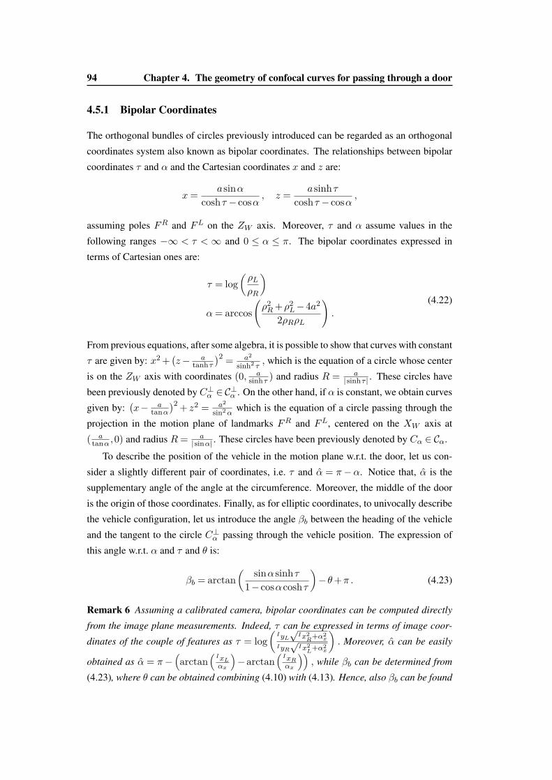
94 Chapter 4. The geometry of confocal curves for passing through a door
4.5.1 Bipolar Coordinates
The orthogonal bundles of circles previously introduced can be regarded as an orthogonal
coordinates system also known as bipolar coordinates. The relationships between bipolar
coordinates τ and α and the Cartesian coordinates x and z are:
x= asinαcoshτ − cosα , z = asinhτ
coshτ − cosα ,
assuming poles FR and FL on the ZW axis. Moreover, τ and α assume values in the
following ranges −∞ < τ <∞ and 0 ≤ α ≤ π. The bipolar coordinates expressed in
terms of Cartesian ones are:
τ = log(ρLρR
)α= arccos
(ρ2R+ρ2
L−4a2
2ρRρL
).
(4.22)
From previous equations, after some algebra, it is possible to show that curves with constant
τ are given by: x2 +(z− a
tanhτ)2 = a2
sinh2 τ, which is the equation of a circle whose center
is on the ZW axis with coordinates (0, asinhτ ) and radius R = a
|sinhτ | . These circles have
been previously denoted by C⊥α ∈ C⊥α . On the other hand, if α is constant, we obtain curves
given by:(x− a
tanα)2 + z2 = a2
sin2αwhich is the equation of a circle passing through the
projection in the motion plane of landmarks FR and FL, centered on the XW axis at
( atanα ,0) and radius R= a
|sinα| . These circles have been previously denoted by Cα ∈ Cα.
To describe the position of the vehicle in the motion plane w.r.t. the door, let us con-
sider a slightly different pair of coordinates, i.e. τ and α = π−α. Notice that, α is the
supplementary angle of the angle at the circumference. Moreover, the middle of the door
is the origin of those coordinates. Finally, as for elliptic coordinates, to univocally describe
the vehicle configuration, let us introduce the angle βb between the heading of the vehicle
and the tangent to the circle C⊥α passing through the vehicle position. The expression of
this angle w.r.t. α and τ and θ is:
βb = arctan( sinαsinhτ
1− cosαcoshτ
)−θ+π . (4.23)
Remark 6 Assuming a calibrated camera, bipolar coordinates can be computed directly
from the image plane measurements. Indeed, τ can be expressed in terms of image coor-
dinates of the couple of features as τ = log(
IyL
√Ix2
R+α2x
IyR
√Ix2
L+α2x
). Moreover, α can be easily
obtained as α = π−(arctan
(IxLαx
)−arctan
(IxRαx
)), while βb can be determined from
(4.23), where θ can be obtained combining (4.10) with (4.13). Hence, also βb can be found

4.5. The Bundle of circles 95
directly from image plane measurements.
4.5.2 Kinematic model of the vehicle in bipolar coordinates
The kinematic model of the vehicle in bipolar coordinates λ= (τ, α, βb) is
τ = ν
a((1 + cos αcoshτ)sin(βb−arccot(cot αcothτ + csc αcschτ))+
+cos(βb−arccot(cot αcothτ + csc αcschτ))sin αsinhτ)˙α= ν
a(−cos(βb−arccot(cot αcothτ + csc αcschτ))(cos αcoshτ + 1)+
+sin αsin(βb−arccot(cot αcothτ + csc αcschτ))sinhτ)
βb =−ω− νa
(cos α+ coshτ)2(cosβb csc α+ cschτ sinβb)(cos α− coshτ)
√1 + (cot αcothτ + csc αcschτ)2
.
(4.24)
Based on (4.20) and (4.21) the maximum value ˙αmax of ˙α is obtained along circles of C⊥α ,
i.e. with βb = 0. By the second of (4.24) we have:
˙αmax = ˙α∣∣∣βb=0
=−ν(cos α+ coshτ)a
. (4.25)
For positive values of ν, the function (4.25), is negative and equal to zero if τ = 0 and
α= π (or α= 0), i.e. very far from the door.
4.5.3 A simple strategy to steer the vehicle through the door exploiting thegeometric properties of the bundle of circles
A strategy to steer the vehicle through the middle of the door follows from these geometric
facts: for any point Q ∈ C⊥α the tangent line to C⊥α passes through the center of the circle
Cα through Q. Moreover, the center of Cα is in turn at the intersection between axis
XW and the circle C2α (i.e. a circle of Cα whose angle at the circumference is 2α). In
particular, the center of circle Cπ/2 coincides with the middle of the door (see Figure 4.4).
Hence, starting from points Q such that α < π/2, a possible strategy is to follow a circle
C⊥α of bundle C⊥α until the circumference characterized by α= π/2 is reached. Then, it is
sufficient to move along a straight line to pass through the middle of the door.
Even though the strategy previously described is able to steer the vehicle through the
middle of the door, it has some drawbacks w.r.t. the feedback control law given by (4.29)
and (4.28). Indeed, while during the first phase a feedback control law guarantees that the
vehicle follows a circle of C⊥α until Cπ/2, during the second phase, a feedforward control
with ω = 0 and u = const. is applied. Moreover, the crossing angle, which is not π/2,
depends on the point reached on the circle Cπ/2. Finally, if at the beginning α > π/2, the

96 Chapter 4. The geometry of confocal curves for passing through a door
vehicle has to reach Cπ/2 backward. Next section is dedicated to the design of a feed-
back control law in bipolar coordinates overcoming all drawbacks of the simple strategy
described in this subsection.
4.6 Feedback Control Law in Bipolar Coordinates
The main idea of designing the feedback control law in bipolar coordinates is to define a
smooth vector field E(·) obtained by derivation of an appropriate potential function F (·).
Let us hence consider the following function:
F (τ, α) = (−cos α+K coshτ)a
, (4.26)
where K is a positive constant. This function is always positive and has a global minimum
at the middle of the door, i.e. when τ = 0 and α = 0 (see also Figure 4.5). Notice that,
function F (·) is very similar to (4.25). Considering F (τ, α) as a potential function, the
associated vector field is:
E(τ, α) =∇F (τ, α) = coshτ − cos αa2
K sinhτ−sin α
. (4.27)
Figure 4.6(a) shows level curves of F (τ, α) as well as the vector field. Notice that, all flow
lines converge toward the point (τ, α) = (0,0), that, in Cartesian coordinates, corresponds
to the middle of the door. In Figure 4.6(b), the same potential field and associated vector
field in Cartesian coordinates is also reported.
The objective is now to determine a feedback control law that steers the vehicle along
the vector field represented in Figure 4.6(a) in bipolar coordinates, or represented in Figure
↵ ⌧-2
0
2
-2
0
2
0
5
10
Figure 4.5: Function F (τ, α) for different values of α and τ and K = 1. The minimum is at theorigin, i.e. at the middle of the door.
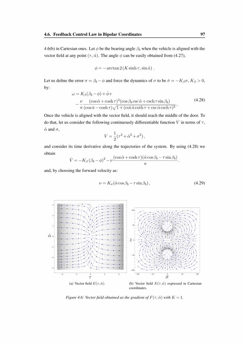
4.6. Feedback Control Law in Bipolar Coordinates 97
4.6(b) in Cartesian ones. Let φ be the bearing angle βb when the vehicle is aligned with the
vector field at any point (τ, α). The angle φ can be easily obtained from (4.27),
φ=−arctan2(K sinhτ, sin α) .
Let us define the error σ = βb−φ and force the dynamics of σ to be σ =−Kβσ, Kβ > 0,
by:ω =Kβ(βb−φ) + φ+
− νa
(cos α+ coshτ)2(cosβb csc α+ cschτ sinβb)(cos α− coshτ)
√1 + (cot αcothτ + csc αcschτ)2 ,
(4.28)
Once the vehicle is aligned with the vector field, it should reach the middle of the door. To
do that, let us consider the following continuously differentiable function V in terms of τ ,
α and σ,
V = 12(τ2 + α2 +σ2) ,
and consider its time derivative along the trajectories of the system. By using (4.28) we
obtain
V =−Kβ (βb−φ)2−ν (cos α+ coshτ)(αcosβb− τ sinβb)a
.
and, by choosing the forward velocity as:
ν =Kν(αcosβb− τ sinβb) , (4.29)
-4 -2 0 2 4
-3
-2
-1
0
1
2
3
↵
⌧(a) Vector field E(τ, α).
-100 -50 0 50 100
-100
-50
0
50
100
x
z
(b) Vector field E(τ, α) expressed in Cartesiancoordinates.
Figure 4.6: Vector field obtained as the gradient of F (τ, α) with K = 1.

98 Chapter 4. The geometry of confocal curves for passing through a door
we finally have:
V =−K1 (βb−φ)2− (cos α+ coshτ)(αcosβb− τ sinβb)2
a≤ 0 ,
which is negative semi-definite. As the function V is positive definite, according to the
Lasalle’s invariance principle, the system trajectories converge to the largest invariant set
R = {λ|V (λ) = 0}. By simple computation, R = R1 ∪R2 where R1 = {λ|{αcosβb−τ sinβb = 0}∩{βb = φ}} and R2 = {λ|{α= 0, τ = 0}∩{βe = φ}}. After simple algebra,
we obtain that R1 = {λ|{α= π}∩{τ = 0}} while R2 = {λ|λ= 0}. It is possible to show
that, if K 6= 0, R1 is not an invariant set. Indeed, for λ = [0, π, 0]T we have ν 6= 0 and
thus the system can escape from R1. As a consequence, the point λ= (0, 0, 0) is the only
invariant set and we can conclude on the local asymptotic stability of the origin. Moreover,
as the Lyapunov function is radially unbounded, we can conclude on the global asymptotic
stability of the origin. Differently from the control law developed in Section 4.4, the control
law developed in this section is able to steer the vehicle exactly through the middle of the
door.
As for hyperbolae and ellipses, each circle of bundleCα intersects each circle of bundle
C⊥α in two points, symmetric w.r.t. the ZW axis. Also the control laws in bipolar coordi-
nates are immune to this fact by following the same reasoning as in Remark 5.
4.7 Simulations
In this section, simulations showing the effectiveness of control laws proposed in Sec-
tions 4.4 and 4.6 are presented. For both cases, two virtual scenario are considered. In
the first one, the robot is inside a room and the objective is to leave the room passing
through the door. In the second one, the robot is in a corridor and the objective is to en-
ter a room passing through the door. The door is represented by two 3D points located
at (0, 70, 40) cm and at (0, 70,−40) cm w.r.t. a global reference frame. These points are
at the same height above the plane of the robot motion. The 3D points of the scene are
projected in the image plane through a simulated pinhole camera. The size of the image
is 640× 480 and the characteristic angle of the camera is almost π. Moreover, the image
frames are captured with a frequency of 15 frames per second. If possible, both elliptic
and bipolar coordinates are computed through image measurements and different levels of
white Gaussian noise with standard deviation σ = 5, 15 pixel to points in the image plane
is also added. Indeed, as in this work the camera is fixed on the robot, it is not possible
in the second scenario (see Figs. 4.8(c) and 4.9(c)) to perform the task without loosing at
least one landmark, even if a very large FOV has been considered. For this reason, in the

4.7. Simulations 99
second scenario we directly assume that elliptic or bipolar coordinates are available and
some white Gaussian noise, equivalent to have a 5 pixel Gaussian noise in the image plane,
is directly added to the state variables.
In Figs. 4.8 and 4.9 trajectories of the vehicle are shown with and without noise
for the two cases, chosen among the several trajectories analyzed for each case. The
absolute average error w.r.t. the middle of the door is also reported in the caption of each
picture with and without noise, i.e. εw and εwo, respectively. The simulations confirm
that both feedback control laws work properly in spite of image noise. Moreover, while
the control law in elliptic coordinates is only able to steer the vehicle near the middle
of the door (the error depends on the constant parameters in the control law), the one
in bipolar coordinates can drive the vehicle exactly to the middle of the door. However,
this is not the only difference. In particular, in bipolar coordinates the behavior of the
vehicle is more suitable to accomplish the task of entering in a room from a corridor.
On the other hand, both methods are able to accomplish the task of going out of a room
even if the trajectories followed by the vehicle are quite different, being more suitable the
one in elliptic coordinates. Indeed, in elliptic coordinates, small variations in the control
parameters traduce in very different shape of the trajectories. However, to reduce as much
as possible the crossing error at the entrance of the door, this parameters should be selected
as a function of the initial conditions. It is important to note that both the control laws in
elliptic and bipolar coordinates guarantee good performance with levels of image noise
up to 15 pixels, which constitutes a very high amount of noise. The use of a feedback
control expressed in elliptic and bipolar coordinates seems to play a very important role in
reducing the effects of noise. Future works will be dedicated to deeply analyze this aspect.
However, the control law in bipolar coordinates seems to be more sensitive to image noise
than the control law in elliptic coordinates when the vehicle is far away from the door,
making difficult the tuning of the control parameters. On the other hand, the control laws
in bipolar coordinates work very well near the door, especially while entering a room from
the corridor. This may suggest a possible strategy: use elliptic control laws when the robot
is far away from the door and bipolar ones when it is sufficiently near the door or when the
vehicle is very near the wall. As a final observation, it is important to point out that, even
if the method relies on the assumption that the two landmarks are at the same height, we
have simulated our method also in case of differences in height up to 10 cm, observing that
the method works quite well also in this case. Both control laws depend on the parameter
a which is half of the width of the door. This parameter is constant and can be assumed
to be known or estimated via a suitable observer. However, Figure 4.7 shows how errors
in the estimation of a influence the trajectories of the vehicle. In particular, starting from
the same configuration, we have considered three cases: a = 40 cm (the actual value),

100 Chapter 4. The geometry of confocal curves for passing through a door
a = 80 cm (twice the actual value) and a = 20 cm (half of the actual value). Simulations
show that errors in the estimation of the parameter a do not compromise the effectiveness
of the control laws. The feedback control law in elliptic coordinates seems to be more
sensitive to variations of the parameter a than the one in bipolar coordinates.
0 50 100 150 200
−80
−60
−40
−20
0
20
40
60
FL
FR
XW [cm]
Z W [c
m]
a = 80
a = 40
a = 20
(a) Control laws in elliptic coordinates developed insection 4.4.
0 50 100 150 200
−80
−60
−40
−20
0
20
40
60
FL
FR
XW [cm]
Z W [c
m]
a = 80
a = 40
a = 20
(b) Control laws in bipolar coordinates developed insection 4.6.
Figure 4.7: Trajectories of the vehicle starting from the same initial configuration q =(200,−50,7π/6), for different values of a in the control law: a = 40 cm (the actual value),a= 80 cm (twice the actual value) and a= 20 cm (half of the actual value).

4.7. Simulations 101
0 100 200 300 400−50
0
50
100
150
200
250
300
350
400
FL
FR
XW [cm]
Z W [c
m]
(a) σ = 5 pixel: εw = 2.00 ± 1.15 cm andεwo = 1.79 ± 1.02 cm.
0 100 200 300 400−50
0
50
100
150
200
250
300
350
400
FL
FR
XW [cm]
Z W [c
m]
(b) σ = 15 pixel: εw = 2.61 ± 1.43 cm andεwo = 1.88 ± 1.03 cm.
−200 −100 0 100 200 300−50
0
50
100
150
200
250
300
350
400
FL
FR
XW [cm]
Z W [c
m]
(c) σ = 5 pixel: εw = 4.43 ± 4.68 cm andεwo ≈ 6.85 ± 2.92 cm.
Figure 4.8: Simulations with the feedback control law in elliptic coordinates: trajectories of thevehicle without and with white Gaussian noise, representing continuous and dashed lines, respec-tively. The vehicle leaves a room in (a), (b) and enters a room from a corridor (c), by passingthrough a door.

102 Chapter 4. The geometry of confocal curves for passing through a door
0 100 200 300 400−50
0
50
100
150
200
250
300
350
400
FL
FR
XW [cm]
Z W [c
m]
(a) σ = 5 pixel: εw = 0.0028 ± 0.096 cm andεwo = 0.0017 ± 0.0011 cm.
0 100 200 300 400−50
0
50
100
150
200
250
300
350
400
FL
FR
XW [cm]
Z W [c
m]
(b) σ = 15 pixel: εw = 0.14 ± 0.70 cm andεwo = 0.0017 ± 0.001 cm.
−200 −100 0 100 200 300−50
0
50
100
150
200
250
300
350
400
FL
FR
XW [cm]
Z W [c
m]
(c) σ = 5 pixel: εw = 0.1 ± 0.33 cm andεwo ≈ 0 cm.
Figure 4.9: Simulations with the feedback control law in bipolar coordinates: trajectories of thevehicle with and without white Gaussian noise, representing continuous and dashed lines, respec-tively. The vehicle leaves a room in (a), (b) and enters a room from a corridor (c), by passingthrough a door.

4.8. Experiments 103
FRFLRobulab 10
On-board camera
Robulab 10
Door
DoorFR FL On-board camera
From behind the door
Figure 4.11: Experimental setup.
4.8 Experiments
Figure 4.10:PT7137 camera
Referring to Figure 4.11, the experimental setup was comprised of a
Vivotek Wireless Network Camera with Pan–Tilt (PT7137) (see Figure
4.10) fixed at the middle of the wheel axis of the RobuLAB–10 (by Ro-
bosoft) mobile platform. The image resolution was 640× 480 and the
camera horizontal and vertical FOV amplitude were around 50 deg and
40 deg, respectively. Moreover, in our experiments, the pan–tilt mech-
anism was not used. The camera was calibrated by the Matlab c© cal-
ibration toolbox. The result of this procedure, has furnished the focal
length: αx = 712.28± 3.32 pixel and αy = 711.93± 3.27 pixel;
the principal point: Pcc = [330.98, 273.42]± [6.69, 6.06] pixel;
the skew: αc = 0, angle of pixel axes is π/2; the distortion:
Kc = [−0.40, 0.24, 0.0018, −0.00011, 0] ± [0.02, 0.09, 0.0015, 0.0012, 0]; the pixel
error: perr = [0.35, 0.29] pixel.
Notice that, the camera presents a radial distortion. The noise level was estimated to have
a standard deviation σ = 0.05 pixel and the controller rate was around 20 Hz. The distance
between the two landmarks was 68 cm.
4.8.1 Technical Details
Without loss of generality and to simplify the experimental setup, we have decided to avoid
the use of door detection algorithms from which the two landmarks characterizing the door
can be obtained. The door is indeed represented by two red circular landmarks at the same
height from the plane of the robot motion. It is important to note that in own approach we
did not implement a door detector algorithm, reasonably assuming that it will be always
possible to determine two points in the image plane corresponding to the doorposts, e.g. the

104 Chapter 4. The geometry of confocal curves for passing through a door
top corners of the door. In the method proposed we assumed that the two landmarks are
at the same height. In case they are not, it is necessary to estimate it. Moreover, in such
case, both bipolar and elliptic coordinates would depend not only on the positions of the
landmarks in the image plane but also on their respective heights. The algorithms have
been developed in C++. Two scripts were run in parallel, communicating with each other
by ROS Hydro. The first one was dedicated to grab an image from the wireless camera
and provide information about the position of the landmarks in the image plan. The second
program was dedicated to receive the information about landmarks and compute the control
inputs ν and ω and to send them to the vehicle. An exhaustive description of the two
programs is provided in the following sections. They are called "Image Processing" and
"Robot Control" algorithm.
Image Processing
The aim of the first program was to read the data from the wireless camera, detect and track
the landmarks. The connection was establish through UDP protocol that allowed real-time
video streams. However, some packets might be lost due to network burst traffic and im-
ages might be obscured. To solve this problem, invalid information were considered as an
exception. If too many of theme occurred (around half second) and the system was not
able to receive correct and valid images, the robot was safety stopped. Since the quality
of the image was really poor (the camera was a web-cam, concerned to remain at a fixed
position, resolution 640x480, 60Hz, frame rate 30 fps), it was necessary to apply several
filtering in order to obtain a robust detection and tracking of the landmarks. We mainly
used OpenCV (version 2.4.9) [Bradski 2000] and ViSP (Visual Servoing Platform, version
2.9.0) [Marchand 2005] libraries. The first step was to convert the image colors from RGB
to HSV space, since the latter has the desirable property to identify a particular color using
a single value (Hue) instead of three. Afterward a Gaussian smoothing was applied to blur
the image and reduce the noise. Since the quality of the data was low and the application
of filters further reduced image details, it was necessary to find an efficient compromise
between noise-reduction and quality. Moreover, a direct detection of the red landmarks
was not the most robust solution since several parameters were required (dimension of the
landmarks, threshold for the edge detector, dimension of the mask for features detection,
parameters of the Gaussian filter) and their values were too dependent on the light condi-
tions of the environment. In order to obtain a robust detection and tracking system of the
landmarks, different approach have been tested. Mainly, we used OpenCV for the detec-
tion of the features and ViSP to track them. Since the landmarks had circular shapes, the
program was made to detect two ellipses.

4.8. Experiments 105
Once they were detected, we used ViSP library for the tracking. If one of landmarks was
lost, the software stopped the tracking and the research of the ellipses started again. Tests
showed that the research was sufficiently fast to maintain the smoothness robot trajectory.
Different approaches were tested and compared to detect and track the landmarks.
Detection : Two approaches were tested based on circles or ellipses detection. Both of
them require to isolated the red color by setting the HSV values (H = [95,145],S = [75,142], V = [90,150]) and turning them to white, while the rest of the pix-
els were set to black. Following this elementary method, we obtained a white and
black image in which the two landmarks were clearly visible. The circle detection
approach was based on the OpenCV function HoughCircles and it provided good per-
formances. However, when the robot was not moving perpendicularly to the door, the
landmarks (that were circles) became more elliptical and the algorithm was not able
to detect them anymore. To solve this problem, we tested a 2-step approach based on
ellipse detection: firstly we used findContours to highlight the landmarks and then
fitEllipse to localize them (the functions are based respectively on [Suzuki 1985] and
[Fitzgibbon 1996] algorithms).
Tracking : OpenCV provides functions to find circles or ellipse and the ViSP library provides
several tools to track objects like moving-edge tracking, template tracking, ellipse
tracking and blobs tracking. After many tests, we found out that blobs tracking
provided the best performance for our task. We used vpDot2 class which requires
the initial position of the blobs that we need to track. To this end, the position
of the two landmarks detected by OpenCV were provided. This approach, even if
it is not direct, allowed us to have a robust tracking system. Although the ViSP
library provides functions to automatically detect circles or ellipses in a image, the
basic OpenCV tools finally guaranteed more robust results for the initial landmarks
detection. However, the tracking task by OpenCV was not smooth, probably due to
the low quality of the image and the noise. We finally concluded that OpenCV ellipse
detector and ViSP blob tracker was the optimal combination for our purpose, given
the limited performance of the camera. In the last step, the position of the landmarks
in the camera plane (u and v coordinates) were sent to the Robot Control algorithm
using ROS Hydro.
106 Chapter 4. The geometry of confocal curves for passing through a door
Robot Control
The aim of this program was to compute the robot control inputs v and ω based on the
landmarks position in the camera plane provided by Image Processing algorithm. The
communication between robot and computer station was established through UDP proto-
col.
The way we controlled the robot is explained in Appendix A. In Image Processing control
we focused only on the landmarks detection and we did not set any kind of control. We
limited the previous algorithm because of computational time limits: image data is quite
heavy and it was necessary to minimize the number of operations. However, several prob-
lems could occur due to such a lack of security control. To this end, the Robot Control
algorithm had to perform several security checks before sending the control signal to the
real robot.
- Image Data validation: if the landmarks were correctly detected, a 6D-vector
m = [u1,v1, r1,u2,v2, r2] was sent from Image Processing to Robot Control
(u1,v1, r1, u2,v2, r2 were respectively the two coordinates in the camera plane and
the ray of the landmarks). However, if the landmarks were not correctly detected, the
vector m was not 6-dimension and the security system had to safety stop the robot
motion. Since the software must provide smooth motion and it is important that the
robot does not hiccup, the angular velocity ω was set to zero and the linear velocity v
remained constant. The idea was that if the landmarks were still in front of the cam-
era and it could be still possible re-detect them, without needing to turn the robot and
then the camera. Regardless, if after half second the landmarks were not re-detected
correctly, the robot was forced to stop.
- Landmark role-assign: The 6-vector m contained information about the two land-
marks. However, there was not a specific order and it was necessary to clarify, be-
fore computing the control law, which information was relative to the left landmark
rather than the right one. A simple check on u coordinates was sufficient to solve
this problem.
- Control inputs: once the control inputs ω and v were computed, a last check was
done to understand if their value were reasonable (if their values were respectively
higher than 1.6 m/s and 2 π). If they were not, the robot was safely stopped.
Because of the limited FOV aperture, the robot lost the landmarks while passing through
the door. Indeed, as shown in the next paragraph, there is a region around the door where
the robot cannot maintain in view the landmarks. To circumvent this problem, in our ex-
periments, the parameters in the control laws were chosen in order to align the vehicle with

4.8. Experiments 107
the line passing through the middle of the door, perpendicularly to the segment [FL,FR],
just before losing the landmarks. Starting from this configuration, which is quite near to the
door, depending on the FOV amplitude, an open loop control law with ω= 0 and ν = const.
was applied. Of course, other solutions might be used. For example, if the heights of the
landmarks were available, by using the last measurements of the landmarks in the image
plane (just before going outside) and the pinhole camera model, a prediction of the future
positions of the landmarks in the image plane could be obtained. These predictions can
be used in the feedback control laws provided in this work to steer the vehicle through the
door even if the landmarks are outside of the image plane. The heights of the landmarks
can be assumed to be known or estimated by a suitable procedure or observer.
4.8.2 Experimental Results
Figure 4.12 and 4.13 report the trajectories of the robot starting from different initial con-
figurations and obtained by applying the feedback control laws based on elliptic and bipolar
coordinates, respectively. The state variables of the robot and hence the trajectories towards
the door have been measured by using the Motion Analysis Capture system. Of course, no
information coming from this sensor system are used in the control laws which provide a
purely Image-Based visual servo control. A video2 of the experiments is available.
2http : //projects.laas.fr/gepetto/uploads/Members/ICRA2015_video.mp4

108 Chapter 4. The geometry of confocal curves for passing through a door
4.9 Analysis of FOV limits
The control laws developed in this work did not take into account the Field–Of–View
(FOV) limits of the on–board camera. In this section we will study and analyze this as-
pect.
Let us first consider the region of points that violate the FOV limits for any orientation
of the robot. In other words, in this region, both landmarks cannot be maintained inside the
FOV, whatever the orientation of the vehicle.
Let γ and γ be the horizontal and vertical FOV aperture, respectively. Because of
horizontal FOV limits, there exists a region Z1 around the door such that the two landmarks
cannot be simultaneously maintained between the left and right bounds of the image plane.
It is straightforward to show (see [Salaris 2010]) that Z1 is bounded by two arcs of circle
(Caγ and Cbγ) whose angle at the circumference is exactly equal to γ (see Figure 4.14(a)).
0 100 200 300 400 500−150
−100
−50
0
50
100
150
200
250
FL
FR
XW [cm]
Z W [c
m]
(a) Trajectories followed by the vehicle.
0 5 10 15 20 250
100
200
300
400
500
600
t [s]
X [c
m]
(b) x.
0 5 10 15 20 25−40
−20
0
20
40
60
80
100
120
140
160
t [s]
Z [c
m]
(c) z
0 5 10 15 20 25−0.2
−0.1
0
0.1
0.2
0.3
0.4
0.5
0.6
0.7
t [s]
θ [ra
d]
(d) θ.
Figure 4.12: Experimental results obtained applying the control law in elliptic coordinates. Thecontrol parameters are w = 0.0012, K = 0.7 and λ = 310, an the average linear velocityv = 0.3 m/s.

4.9. Analysis of FOV limits 109
Because of vertical FOV limits, considering each landmark separately, there is a re-
gion around it that the vehicle cannot reach while maintaining the landmark between
the upper and lower bounds of the image plane. Also in this case, it is easy to show
(see [Salaris 2015a]) that this regions is bounded by two circumferences (CRγ and CLγ for
the right and left landmark) centered at the projection of the landmark on the motion plane
and with radius equal to Rb = htan(γ/2) (see Figure 4.14(b)). However, if we consider the
problem of maintaining both landmarks between the upper and lower bounds of the image
plane, the region Z2 that the vehicle cannot reach is a planar capsule delimited by two
straight lines sI and two semicircle ends (see Figure 4.14(b)). This is a direct consequence
of the fact that when the landmark is on the upper (or lower) bound of the image plane,
the vehicle is aligned with the tangent to the involute of circle passing through the current
position of the vehicle (see [Salaris 2015a]). These involute of circles, named by IR and
IL (see Figure 4.14(b)), have CRγ and CLγ , respectively, as base circles. When both features
0 100 200 300 400 500−150
−100
−50
0
50
100
150
200
250
FL
FR
XW [cm]
Z W [c
m]
(a) Trajectories followed by the vehicle.
0 5 10 150
100
200
300
400
500
600
t [s]
X [c
m]
(b) x.
0 5 10 15−20
0
20
40
60
80
100
120
140
160
180
t [s]
Z [c
m]
(c) z
0 5 10 15−3.4
−3.3
−3.2
−3.1
−3
−2.9
−2.8
−2.7
−2.6
−2.5
t [s]
θ [ra
d]
(d) θ.
Figure 4.13: Experimental results obtained applying the control law in bipolar coordinates. Thecontrol parameters are K = 2, K1 = 4 and Kν = 0.15. Average linear velocity of 0.4 m/s.
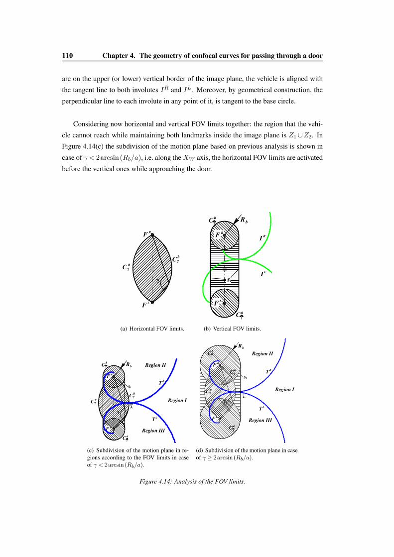
110 Chapter 4. The geometry of confocal curves for passing through a door
are on the upper (or lower) vertical border of the image plane, the vehicle is aligned with
the tangent line to both involutes IR and IL. Moreover, by geometrical construction, the
perpendicular line to each involute in any point of it, is tangent to the base circle.
Considering now horizontal and vertical FOV limits together: the region that the vehi-
cle cannot reach while maintaining both landmarks inside the image plane is Z1 ∪Z2. In
Figure 4.14(c) the subdivision of the motion plane based on previous analysis is shown in
case of γ < 2arcsin(Rb/a), i.e. along theXW axis, the horizontal FOV limits are activated
before the vertical ones while approaching the door.
(a) Horizontal FOV limits. (b) Vertical FOV limits.
(c) Subdivision of the motion plane in re-gions according to the FOV limits in caseof γ < 2arcsin(Rb/a).
(d) Subdivision of the motion plane in caseof γ ≥ 2arcsin(Rb/a).
Figure 4.14: Analysis of the FOV limits.

4.9. Analysis of FOV limits 111
4.9.1 Control strategy in case of FOV limits
From the previous section, it is clear that the vehicle cannot reach the middle of the door
while maintaining both landmarks in sight. To avoid this problem, the control law devel-
oped in Section 4.6 can be modified in order to reach the configuration λ= [0, π−γ, 0]T ,
i.e. point λ in Figure 4.14(c), instead of the configuration λ= [0, π, 0]T . This can be done
by considering the modified potential function
Fγ(α, τ) = (−cos(α− (π− δ)) +K coshτ)a
and vector field
Eγ(τ, α) = coshτ − cos(α− (π− δ))a
K sinhτ−sin(α− (π− δ))
.and finally the following candidate Lyapunov function
V = 12(τ2 + (α− (π− δ))2 +σ2
), (4.30)
where δ = γ. Once the vehicle reaches λ, an open loop control can be applied, e.g. with
controls ν = const. and ω = 0. However, especially from a practical point of view, de-
pending on both the value of γ (and hence the distance between the reached point and the
door) and the final error which depends also on the image noise, this strategy might steer
the vehicle very far from the middle of the door. In this case, an estimation of the landmark
positions based on the camera model can be used until a new pair of landmarks is available.
To do that, the height of the landmarks must be known, e.g. from an observer that estimates
h during the first phase, in which the vehicle is approaching λ. Once h is obtained, it can
be used to estimate landmark positions on the image plane (even though their are outside
it) that can be in turn used in the feedback control laws.
Finally, when the vehicle is sufficiently far from the door, the horizontal limits
of the FOV become more restrictive than the vertical ones. From results reported
in [Salaris 2010], when the landmark moves on the right or on the left border of the image
plane, the vehicle moves along a logarithmic spiral rotating counterclockwise or clockwise,
respectively, around the projection on the motion plane of the landmark position. Depend-
ing on the value of γ, there exist two logarithmic spirals, TR and TL in Figure 4.14(c),
passing through λ, whose characteristic angle3 is constant and equal to γ/2. The spirals
are tangent in (τ, π− γ) and subdivide the motion plane in three regions. Referring to
3Given a point Q= (ρQ,ψQ) on a logarithmic spiral rotating around point OW , the characteristic angle isthe angle between the tangent to the spiral in Q and the radial line at the point Q.

112 Chapter 4. The geometry of confocal curves for passing through a door
Figure 4.14(c), starting from Region II and III with an orientation such that both landmarks
are in view, the vehicle cannot reach point λ while maintaining both landmarks inside the
FOV along the whole trajectory. From these regions, a preliminary maneuver that steers
the vehicle in Region I is needed to achieve the task. Indeed, from Region I the control
law obtained from (4.30) might be able to steer the vehicle in λ by appropriately choosing
the control parameters. If one feature reaches the right or left border of the image plane,
the vehicle can move along the logarithmic spiral until point λ is reached. In this case, the
value of δ to be used in the Lyapunov function (4.30) is 2arcsin(Rb/a). Previous analysis
is valid even if Rb ≥ asin(γ/2), or γ ≥ 2arcsin(Rb/a). In this case, the point λ is in
the middle of the line sI where logarithmic spiral are not tangent (see Figure 4.14(d)). In
particular, if γ = π, Caγ and Cbγ reduce to the segment FRFL while the logarithmic spirals
become two circles centered at the projection on the motion plane of each landmark and
passing through the middle of the door.
4.10 Conclusions
In this chapter, a geometric approach to steer a robot subject to nonholonomic constraints
through a door by using visual measures coming from a fixed on-board monocular camera,
has been provided. The planar geometry that, in a natural way, has been built around the
door consists of bundle of hyperbolae, ellipses and orthogonal circles. The method pro-
posed is able to accomplish such an task through static feedback control laws that are func-
tions of the current state of the system expressed in suitable coordinate, directly measured
in the camera plane. Indeed, our approach does not consist in a pre-planned path among
via-points or a multi-stage strategy. Therefore, we avoid the computational cost of a state
observed that would require to localize the robot. Realistic simulations and experiments
have been also reported to show that the method proposed is robust against disturbances
and uncertainties.

Conclusion and Perspectives


115
The first part of this thesis work has been done within the framework of the Euro-
pean project KoroiBot which aimed to improve humanoid robots capabilities inspired by
humans. In this context, we investigated some principles that underlie the organization
of human walking, with the aim to transfer them to humanoid robots. Our work in this
direction gave rise to two main contributions. First, in collaboration with specialists in
crowd simulation and motion planning at INRIA-Rennes, we investigated the human prin-
ciples which guide collision avoidance strategies during goal-directed locomotion. Then,
in collaboration with our KoroiBot partner from Tübingen, we proposed a novel approach
to synthesize realistic complex humanoid robot movements based on motion primitives.
Aside the KoroiBot project, we had an internal collaboration at LAAS-CNRS with Paolo
Salaris and Jean-Paul Laumond which led a the third contribution. It concerns the synthesis
of vision-based controllers based on original parametrization for passing through a door.
This work has been supported by European Research Council within the ERC Actanthrope.
The outcomes related to these three contributions are detailed below. Some perspectives
are developed in each case.
Identification of human walking strategies for avoiding a moving obstacle
One of the first steps of our study has been to record humans walking motions in order to
investigate and identify the natural and biological strategies to avoid a moving obstacle.
The main idea was to create situations for which the behavior of the walker was consid-
erably perturbed by an external agent. To this aim, we programmed a wheeled robot that
had to cross the pedestrian path. Considering the related works on this topic, we started
a collaboration with specialists on human locomotion at INRIA-Rennes. They previously
investigated the strategies used by two pedestrians crossing each other and they found out
that both participants were able to predict the future crossing order. Moreover, it turned out
that the collision avoidance is collaboratively performed by both participants and that the
walker giving way contributes more than the one passing first. They concluded that it exists
a natural tacit understanding of roles which guides humans avoidance strategies. In order
to determine if those observed principles could be extended to the case of a human crossing
a moving robot, we reproduced the same experimental setup by replacing one of the walk-
ers by a wheeled robot. Initially, we considered the robotic platform TurtleBot4 that has
open-source software and it is well known in the scientific community. However, due to
its limited speed and dimensions, we observed that the behavior of the participants was not
sufficiently perturbed. For this reason, we considered the wheeled robot Robulab10 that is
heavier and faster.
4http://www.turtlebot.com/

116 Conclusion and Perspectives
In the first part of this study we decided to control the robot in a passive way. The word
"passive" means that the robot is moving straight at constant speed and it is not reacting to
the participant adaptations. All the analyzes were based on the concept of signed minimal
predicted distance (smpd), which provides information about the future crossing order
given the position, the velocity and the orientation of both agents. Since the speed and
the direction of the moving obstacle were set constant, only the walker contributed to
solve the collision avoidance. In this case we observed that humans preferentially give
way to the robot, even though this choice is not optimal to avoid collision. Moreover,
humans never decided, in the cases in which they were second in the crossing order, to
accelerate and pass as first. We correlated this behavior to the notion of danger and safety,
hypothesizing that during walking the humans set some prioritized sub-tasks as reaching
the goal, scanning the environment, avoiding obstacles, etc. The conservative strategy
observed led to conclude that avoiding the collision and, in particular, the preservation
of the personal space, are the sub-tasks with higher priority during walking. From these
observations, we concluded that, since the robot is not reacting but keeps moving straight,
the participants did not feel comfortable to interact with it and, sometimes, they could
have been even surprised. In addition, since the pedestrian is the only one to solve the
collision avoidance then the task requires more effort from his side. Finally, it results that
the passive behavior of the robot is somehow counterintuitive for the human.
In the second part of this study, having in mind the results observed in the passive
case, we reproduced the same experimental setup but by controlling the robot in a reactive
way. Our goal was to observe the human behavior in this case and compare with the ones
previously examined. In order to be cooperative, the robot was programmed to follow the
avoidance strategies observed in humans when crossing each other: accelerating at the be-
ginning of the interaction and then turning to pass ahead the participant or decelerating and
turning to pass behind . The results showed that the comfort of the walkers was improved:
they solved all the tasks (reaching the goal and the collision avoidance) with smoother
adaptation and their behavior was more natural. We interpreted this phenomenon by the
fact that it is easier for the pedestrian to understand the ongoing situation when the robot
is taking decision too in a human-like way. This outcome is reasonable if we correlate the
concept of implicit strategies for collision avoidance: people interact with each other daily
and they do it almost the same way. These adaptations are optimized, learned and improved
by our life experience. For these reason, it is easier for a walker to predict how to solve
collision avoidance if the robot is acting like a human.

117
Future Works
The conclusion of these two studies opens path for future research. We addressed ques-
tions as: Do humans understand when a robot is cooperating rather than passive? Do they
adapt their strategies accordingly? Is it useful to transfer human locomotion strategies to
an autonomous robot? We observed that the humans behave more naturally if the robot
moves in a human-like way and the collision avoidance is bilaterally solved, mainly at the
beginning of the reaction phase. No extreme changes of direction or drastic speed variation
are needed to make humans understand the robot intentions. Given these results, we raise
new questions: would it be possible to further improve the comfort of the humans if the
robot would have humans aspects? This concept could be even related to the challenge
of integrating humanoid robots in the human society. Assuming that humanoid robots of
the future will have communication skills similar to the human ones, it is normal to hy-
pothesize that we could maximize the use of such abilities to better succeed the collision
avoidance task. In fact, pedestrians interact each other mainly in two ways: verbal and non-
verbal communication. Normally, some basic postures (or body messages) are sufficient
to clearly show own intentions. However, in wavering situation, it is often necessary to
perform more showy movements, e.g. stepping laterally ("I am going left/right"), stopping
and waiting ("I am giving way to you"), performing longer steps and accelerating ("I am
passing as first"). Hand signals, face expressions, eyes contact are also common methods
to communicate with others. Although people may talk, that would be the faster and easier
way, the lack of confidentiality led to have more nonverbal messages. Given these observa-
tions, which level of communication would be optimal to have an exhaustive understanding
in terms of locomotion strategies? Which actions could make easier the collision avoidance
for humans? Would it be faster to adapt and behave naturally with humanoid robots, if they
use gestures and/or they talk during an interact? or people would be frightened because it
is unnatural? We believe that the work we have done in Chap. 1 and Chap. 2 could serve
as an interesting basis for addressing these questions with humanoid robots.
Use of motion primitives to implement complex movements on humanoidrobots
In Chap. 3 we proposed a whole body controller based on movement primitives extracted
from human behavior. This work has been done in collaboration with our neuroscientists
partners from Tübingen in the framework of the KoroiBot project. The considered no-
tion of motion primitive was defined in space and in time and based on kinematic data
acquired by a motion capture system [Giese 2009b, Mukovskiy 2013]. In this context, ten
trajectories of a human during walking-to-grasp tasks have been recorded. Since humans

118 Conclusion and Perspectives
and humanoid robots are different in terms of size, step lengths, joint limits, torque limits,
etc., the recorded whole body movements have been rescaled and retargeted in order to
match the kinematics of the humanoid robot HRP-2. Once the scaled motions were ob-
tained, we extracted the joint trajectories and then we segmented and normalized them in
terms of time. The step lengths were analyzed too but they were stored separately. At
this point, two subsets of trajectories were collected: one concerning the pelvis linear and
angular velocity and the other one related to the upper-body configurations. In order to
learn low-dimensional representations of each segmented motion, we applied the anechoic
demixing algorithm. By this method, all the trajectories could have been represented as
a linear weighted superpositions of source signals shifted in time. To represent the entire
walking-to-grasp movement, we used a total of five periodic source signals and two nonpe-
riodic ones. Since the trajectories generated for the legs did not provide stable walking for
our robotic platform, we decided to use the walking pattern generator and the related dy-
namic filter developed at LAAS-CNRS roughly described in Section 3.2.3. In conclusion,
the control of the lower body was driven by the pelvis trajectory whereas the upper-body
was controlled by the motion primitives extracted from human data. The global task was
divided in three phases. In the first one, three steps were generated to reach the object to
grasp. If they were not sufficient to arrive at the target, additional steps were automatically
introduced. For this first action, three source signals have been considered. The second
phase consists in approaching the target: the robot has to decelerate and stop at the optimal
distance for grasping the object. To model this action and the third phase, which required
adaptive steps and upper body motion for grasping, we added two periodic sources. The
proposed algorithm has been tested in realistic simulation (OpenHRP2) and in the real
humanoid robot HRP-2. It resulted that all the motions generated were feasible.
Future Works
As a future work, it could be interesting to extend the training set which should include
some additional motion data that maximize the variation of parameters for each individual
action. The training set will have to contain only feasible behaviors, that are extracted
directly from the robot simulator. In other words, instead of building the training set with
the human data, we propose to use the joint trajectories computed by the generalized inverse
kinematics in the Stack of Tasks. In this way, the learning process would be based on
feasible data and it would provide motions that are more appropriated. Moreover, the
learning process should take into account that the pitch joint of the chest is fixed to zero
and that the ground could be not flat. Since the joint trajectories in the training set are
extracted from feasible motion, the generated movements from the learning process should

119
be more dynamically stable for the robot and increase the flexibility and computational
efficiency of the proposed architecture. It would be also interesting to record other kinds
of actions and test them based on the same algorithm.
Vision-based control to pass though a door
In Chap. 4 we described a novel vision-based control to steer a robot to pass through a
door. We considered a nonholonomic wheeled robot that was equipped with a fixed on-
board monocular camera. In the proposed approach, we built around the door a planar
geometry of bundle of hyperbolas, ellipses and orthogonal circles. The method is able to
steer the vehicle through the door by static feedback control laws that are function of the
current state of the system expressed in suitable coordinates that can be directly measured
in the camera image plane. In other word, given the position of the two landmarks in the
image plane, our method is able to directly provide the control inputs to steer the vehicle
to accomplish the task. Therefore, our approach avoids the computational cost of a state
observer that would require to localize the robot with respect to the goal. In this work, the
theoretical contribution consists in elaborating two feedback control laws, in elliptic and
bipolar coordinates respectively. Both controllers have been tested in simulation and on
the real robot. The experimental results confirmed that both feedback control laws work
properly in spite of image noise. Moreover, while the control law in elliptic coordinates is
only able to steer the vehicle near the middle of the door, the one in bipolar coordinate can
drive the vehicle exactly to the middle of the door. This is not the only major difference.
In fact, in bipolar coordinates the behavior of the vehicle is more suitable to accomplish
the task of entering inside the door from a corridor, whereas the elliptic coordinates pro-
vide more suitable trajectory to move close to the door. Although both methods guarantee
good performance despite image noise, the control law in bipolar coordinates turns out
to be more sensitive to noise than the elliptic one if the vehicle is distant from the door,
making difficult the tuning of the control parameters. We conclude that an optimal strategy
might be to use the elliptic control law when the robot is far from the door and then switch
to bipolar strategy when it is sufficiently close to it or when it is really near the adjacent
walls.
Future Works
This work can be easily extended to other navigation and control problems, as e.g. con-
trolling the vehicle amidst obstacles, under the condition that pairs of features correspond
to the 3D position of the obstacles and that they can be extracted from the image
plane. The vision-based strategy presented in this work can also be related to human

120 Conclusion and Perspectives
locomotion. In [Mombaur 2010], by modeling the human locomotion as a unicycle
[Arechavaleta 2008], an inverse optimal control approach was used for understanding
the cost functional that humans minimize during a rest–to–rest task, as e.g. to approach
a door. The results enlighten the role of the bearing angle, and by consequence the role
of vision, in the formation of locomotor trajectories. In Figure 4.15(c) some examples
of trajectories followed by humans are reported. Subjects, starting from the same initial
configuration, have to reach different final positions with the same orientation, i.e. 120 deg
in Figure 4.15(c). We reproduced the similar experiment by simulating the unicycle vehicle
controlled by the feedback control laws in elliptic and bipolar coordinates developed in
Chap. 4. Results of this simulation are reported in Figs. 4.15(a) and 4.15(b). Strikingly
the trajectories followed by the vehicle resemble the human ones. As a future work it
should be interesting to continue the study in this direction and evaluate the effect of
varying the different control parameters. It would be also interesting to introduce a pan–tilt
mechanism to take into account that humans can turn the head and gaze [Hicheur 2005].
However, when a human subject goes toward a target at a constant velocity it is shown that
he behaves as a nonholonomic system: its velocity remains roughly tangent to its sagittal
plane [Arechavaleta 2008].
For all these reasons, it would be interesting to integrate this methodology in walking
pattern generators to steer humanoid robots, e.g. the HRP-2, towards a target. In particu-
lar, it would be interesting to study how the proposed planar geometry allows to combine
both the bearing angle and the focus of expansion to generate a visual feedback control of
locomotion as humans do [Warren 2001].

121
−200 −100 0 100 2000
100
200
300
400
500
600
700
800
900
Z W [c
m]
XW [cm]
(a) By elliptic coordinates.
−200 −100 0 100 2000
100
200
300
400
500
600
700
800
900
Z W [c
m]
XW [cm]
(b) By bipolar coordinates.
The point of view addressed in this paper differs from theprevious ones. We do not consider neither the sensory in-puts nor the complexity of mechanical system modeling thehuman body. The point of view is complementary and moremacroscopic than the standard biomechanics approaches.We want to take advantage of the observation of the shapeof the locomotion trajectories in the simple 3-dimensionalspace of both the position and the orientation of the body.We show that the shape of the human trajectories can bedescribed by a simple differential system. The differentialmodel we propose opens an original bridge between theresearches performed in the human physiology and themathematical background developed on the nonholonomicsystems in mobile robotics. This point of view consti-tutes the first contribution of the paper. The most popularnonholonomic system is a rolling vehicle. This vehiclerolls without sliding. This non-sliding constraint definesthe distribution of Eq. (1). Motion planning and control forrolling vehicles is an active research area in mobile robotics[2], [8]. The controls of a vehicle are usually the linearvelocity (via the accelerator and the brake) and the angularvelocity (via the steering wheel). The question addressedin this paper can be roughly formulated as: where is the“steering wheel” of the human body located? Several bodyframes have been considered on the human skeleton (head,pelvis and trunk). The conclusion of our experimental studyis to show, first that there exists a body frame that accountsfor the nonholonomic nature of the human locomotion andsecond that the trunk is the best “steering wheel” comparedto the head and the pelvis.
The following section presents the experimental proto-col. This protocol is original. This is the first one thatconsiders the problem of the shape of the human loco-motion trajectories just defined by a goal to be reachedin both position and orientation. Then we present the dataanalysis and processing in Section III. A comparative studyinvolving head, pelvis and trunk frames is presented inSection IV. The differential model of Eq. (1) is instantiatedwith the trunk frame in Section V. By integrating such adifferential model we show that the simulated trajectoriesfit with the real ones from a statistical study including 1,560trajectories performed by seven subjects. The conclusiondevelops the interest of the proposed differential model forfuture research directions.
II. APPARATUS AND PROTOCOL
We used motion capture technology to record the trajec-tories of body movements. Subjects were equipped with 34light reflective markers located on their head and bodies.The sampling frequency of the markers was 120 Hz usingan optoelectronic Vicon motion device system (Vicon V8,Oxford metrics) composed of 24 cameras. It is importantto mention that we do not apply any kind of filter to rawdata in our analysis (see Fig. 1).
(a) (b)
(c) (d)
Fig. 1. Some examples of actual trajectories with the same finalorientation. (a), (b), (c) and (d) show all actual trajectories where thefinal orientation is 330 deg., 120 deg., 90 deg. and 270 deg. respectively.
To examine the geometrical properties of human loco-motor paths, actual trajectories were recorded, in a largegymnasium in seven normal healthy males who volunteeredfor this study. Their ages and heights ranged from 25 to30 years and from 1.60 to 1.80 m respectively.
In order to specify the position of the subject on the planewe established a relationship between the laboratory’s fixedreference frame and the trajectory’s reference frame whichcan be computed using either head, trunk or pelvis markersas we explain in Section III. Hence, the configuration A ofthe subject is described as a 3-vector (xa, ya, θa).
(c) By humans (From [Arechavaleta 2008],courtesy of the authors).
Figure 4.15: Some examples of trajectories with the same final orientation, generated by the con-trol laws in elliptic and bipolar coordinates and by Humans. In (a), (b) and (c) the final orien-tation is 120 deg. (a) By elliptic coordinates. (b) By bipolar coordinates. (c) By humans (from,[Arechavaleta 2008] courtesy of the authors).


APPENDIX A
Mobile Robot Robulab10


A.1. Robulab10 Motion Control 125
A.1 Robulab10 Motion Control
In this appendix we present the technical details about the wheeled robot Robulab from
RobuSoft and the methods used to control it. The software that is going to be presented
was developed as basis to implement the tracking control exploited in Chap. 1 and Chap. 2
and the vision-based control laws described in Chap. 4.
A.1.1 The robotic platform
Robulab10 is a multi-purpose mobile robot designed to embed various "applications mod-
ules". It is a generic base plate (platform) industrialized to be used for various applications
thanks to the additional modules that can be integrated, e.g. a Pant–Tilt camera on the top.
The robot is equipped with an internal computer called RobuBOX that provides different
features i.e. manual remote control by joypad, obstacle detection, wire or wireless control.
Although the control of the robot is mainly developed for Microsoft Robotics Studio, also
some basic functions, needed by most of automatic guided vehicles, are provided. In par-
ticular, it is possible to control the robot by a remote station by a wireless communication
through an UDP connection.
(a) (b)
Figure A.1: (a) The basic version of Robulab10 and (b) the one with the Pan–Tilt camera PT7137mounted on the top used for the experiments.
Dimension 450 x 400 x 243 mm. (L x W x H)Payload 30 KgWeight 20 Kg, including batteries
Max speed 4 m/sCommunication Wi-Fi and LAN
Table A.1: Main technical features of Robulab10.

126 Appendix A. Mobile Robot Robulab10
A.1.2 Robot Remote Control
In order to control the robot we connected our remote station through wi-fi connection and
we send low-level messages by an UDP connection. These messages have to be sent with
a particular order. To define the priority of the messages, we have to specify their priority
by some square brackets. An example is reported below. The principal commands are:
n Alive : needed to avoid that WatchDog1 stops the robot;
n Start : it allows to set the robot in remote-control mode;
n Drive : it is the move command. The linear and and angular velocity must be ex-
pressed in cm/s and rad/sec.
Example: to move the robot straight at 1.4 m/s, instructions that have to be sent ( f = 50Hz):
[1] Alive[2] Start[3] Drive 140 0
The programming language considered was C++. I created the class Robulab10 that
had to be defined at the beginning of the program. The class provided three main methods:
ä establish_connection() : it checks and creates the sockets to establish the UDP con-
nection. The IP address of the robot must be defined inside this function in order to
send the message. This method must be called just after the definition of the class;
ä move_robot(double lin_vel, double ang_vel) : to send the control inputs;
ä stop_robot() : it stops immediately the robot;
The code aims to be user-friendly and open source 2. Unfortunately, the official documen-
tation is not anymore available and it has not been possible to improve further the software
with new functions. The code developed can be used by any user and can be integrated
with other communications e.g. ROS and YARP. In our experiments, we used ROS to
communicate with the MoCap (Vicon or Motion Analysis) for obtaining the robot position
and orientation. Therefore, we computed the robot inputs by using path following con-
trol (predefined path) or tracking control (reference behavior). The developed software is
compatible and tested with ROS Groovy, Hydro and Indigo version.1The WatchDog, sometimes called as computer operating properly timer, is an electronic timer that is used
to detect and recover from computer malfunctions. The WatchDog in Robulab10 checks every 800ms if therobot is in "Alive" mode or not. If it is not, the robot is stopped.
2https://github.com/Christian-Vassallo/robot_follow_mocap/blob/master/src/Robulab10Class.hpp

Bibliography
[Aicardi 1995] M. Aicardi, G. Casalino, A. Bicchi et A. Balestrino. Closed loop steering
of unicycle like vehicles via Lyapunov techniques. IEEE Robotics & Automation
Magazine, vol. 2, no. 1, pages 27–35, 1995. (Cited in page 90.)
[Ajallooeian 2013] M. Ajallooeian, J. van den Kieboom, A. Mukovskiy, MA. Giese et AJ.
Ijspeert. A general family of morphed nonlinear phase oscillators with arbitrary
limit cycle shape. Physica D: Nonlinear Phenomena, vol. 263, pages 41–56, 2013.
(Cited in page 63.)
[Ajoudani 2014] A. Ajoudani, J. Lee, A. Rocchi, M. Ferrati, EM. Hoffman, A. Settimi,
DG Caldwell, A. Bicchi et NG. Tsagarakis. A manipulation framework for compli-
ant humanoid COMAN: Application to a valve turning task. In Humanoid Robots
(Humanoids), 2014 14th IEEE-RAS International Conference on, pages 664–670,
2014. (Cited in page 62.)
[Albrecht 2012] S. Albrecht, P. Basili, S. Glasauer, M. Leibold et M. Ulbrich. Modeling
and analysis of human navigation with crossing interferer using inverse optimal
control. IFAC Proceedings Volumes, vol. 45, no. 2, pages 475–480, 2012. (Cited
in page 42.)
[Arechavaleta 2008] G. Arechavaleta, JP. Laumond, H. Hicheur et A. Berthoz. On the
nonholonomic nature of human locomotion. Autonomous Robots, vol. 25, no. 1-2,
pages 25–35, 2008. (Cited in pages xi, 120 et 121.)
[Atkeson 1997] CG. Atkeson, AW. Moore et S. Schaal. Locally Weighted Learning. A.I.
Review, vol. 11, pages 11–73, 1997. (Cited in page 68.)
[Basili 2013] P. Basili, M. Saglam, T. Kruse, M. Huber, A. Kirsch et S. Glasauer. Strate-
gies of locomotor collision avoidance. Gait and posture, vol. 37, no. 3, pages
385–390, 2013. (Cited in pages 19 et 42.)
[Bhattacharya 2007] S. Bhattacharya, R. Murrieta-Cid et S. Hutchinson. Optimal paths
for landmark-based navigation by differential-drive vehicles with field-of-view con-
straints. IEEE Transactions on Robotics, vol. 23, no. 1, pages 47–59, 2007. (Cited
in page 81.)
[Boyd 2004] Stephen Boyd et Lieven Vandenberghe. Convex optimization. Cambridge
university press, 2004. (Cited in page 71.)

128 Bibliography
[Bradski 2000] G. Bradski. Dr. Dobb’s Journal of Software Tools, 2000. (Cited in
page 104.)
[Brandao 2013] M. Brandao, L. Jamone, P. Kryczka, N. Endo, K. Hashimoto et A. Takan-
ishi. Reaching for the unreachable: integration of locomotion and whole-body
movements for extended visually guided reaching. In Proc. of 13th IEEE-RAS Int.
Conf. on Humanoid Robots (Humanoids), pages 28–33, 2013. (Cited in page 63.)
[Breazeal 2005] C. Breazeal, CD. Kidd, AL. Thomaz, G. Hoffman et M. Berlin. Effects of
nonverbal communication on efficiency and robustness in human-robot teamwork.
In 2005 IEEE/RSJ International Conference on Intelligent Robots and Systems,
pages 708–713. IEEE, 2005. (Cited in page 41.)
[Brockett 1983] RW. Brockettet al. Asymptotic stability and feedback stabilization. Dif-
ferential geometric control theory, vol. 27, no. 1, pages 181–191, 1983. (Cited in
page 89.)
[Buchli 2006] J. Buchli, L. Righetti et AJ. Ijspeert. Engineering Entrainment and Adapta-
tion in Limit Cycle Systems - from biological inspiration to applications in robotics.
Biol. Cyb., vol. 95, no. 6, pages 645–664, 2006. (Cited in pages 62 et 67.)
[Buss 2011] M. Buss, D. Carton, B. Gonsior, K. Kuehnlenz, C. Landsiedel, N. Mit-
sou, R. de Nijs, J. Zlotowski, S. Sosnowski, E. Strasseret al. Towards proac-
tive human-robot interaction in human environments. In Cognitive Infocommu-
nications (CogInfoCom), 2011 2nd International Conference on, pages 1–6. IEEE,
2011. (Cited in page 41.)
[Carelli 2002] R. Carelli, C. Soria, O. Nasisi et E. Freire. Stable AGV corridor naviga-
tion with fused vision-based control signals. In IECON 02 [Industrial Electronics
Society, IEEE 2002 28th Annual Conference of the], volume 3, pages 2433–2438.
IEEE, 2002. (Cited in page 81.)
[Carton 2013] D. Carton, A. Turnwald, D. Wollherr et M. Buss. Proactively approaching
pedestrians with an autonomous mobile robot in urban environments. In Experi-
mental Robotics, pages 199–214. Springer, 2013. (Cited in pages 20, 41 et 58.)
[Carton 2016] D. Carton, W. Olszowy et D. Wollherr. Measuring the Effectiveness
of Readability for Mobile Robot Locomotion. International Journal of Social
Robotics, pages 1–21, 2016. (Cited in page 42.)

Bibliography 129
[Chang 2001] CC. Chang et CJ. Lin. LIBSVM: a library for support vector machines,
2001. Software available at http://www.csie.ntu.edu.tw/~cjlin/
libsvm. (Cited in page 67.)
[Chaumette 2006] F. Chaumette et S. Hutchinson. Visual servo control. I. Basic ap-
proaches. IEEE Robotics & Automation Magazine, vol. 13, no. 4, pages 82–90,
2006. (Cited in page 83.)
[Chaumette 2007] F. Chaumette et S. Hutchinson. Visual servo control, Part II: Advanced
approaches. IEEE Robotics and Automation Magazine, vol. 14, no. 1, pages 109–
118, 2007. (Cited in page 83.)
[Cheein 2009] FA. Cheein, C. De La Cruz, R. Carelli et TF. Bastos-Filho. Solution to a
door crossing problem for an autonomous wheelchair. In 2009 IEEE/RSJ Inter-
national Conference on Intelligent Robots and Systems, pages 4931–4936. IEEE,
2009. (Cited in page 82.)
[Cheein 2010] F. Cheein, C. De La Cruz, T. Bastos et R. Carelli. Slam-based cross-a-door
solution approach for a robotic wheelchair. Int J Adv Robot Syst, vol. 7, no. 2,
pages 155–164, 2010. (Cited in page 82.)
[Chiovetto 2013] E. Chiovetto, A. d’Avella, D. Endres et MA. Giese. A unifying algo-
rithm for the identification of kinematic and electromyographic motor primitives.
Bernstein Conference, vol. 0, page 0, April 2013. not reviewed. (Cited in pages 66
et 67.)
[Cinelli 2007] ME. Cinelli et AE. Patla. Travel path conditions dictate the manner in
which individuals avoid collisions. Gait and Posture, vol. 26, no. 2, pages 186–
193, 2007. (Cited in page 20.)
[Cinelli 2008] ME. Cinelli et AE. Patla. Locomotor avoidance behaviours during a visu-
ally guided task involving an approaching object. Gait and posture, vol. 28, no. 4,
pages 596–601, 2008. (Cited in page 20.)
[Dai 2013] DW. Dai, GL. Jiang, J. Xin, X. Gao, LL. Cui, YS Ou et GQ. Fu. Detecting,
locating and crossing a door for a wide indoor surveillance robot. In Robotics and
Biomimetics (ROBIO), 2013 IEEE International Conference on, pages 1740–1746.
IEEE, 2013. (Cited in page 82.)
[Dalibard 2013] S. Dalibard, A. El Khoury, F. Lamiraux, A. Nakhaei, M. Taïx et JP. Lau-
mond. Dynamic Walking and Whole-Body Motion Planning for Humanoid Robots:

130 Bibliography
an Integrated Approach. Int. Journal of Robotics Research, vol. 32, no. 9-10, pages
1089–1103, 2013. (Cited in page 63.)
[Dedieu 2000] D. Dedieu, V. Cadenat et P. Souères. Mixed camera-laser based control for
mobile robot navigation. In Intelligent Robots and Systems, 2000.(IROS 2000).
Proceedings. 2000 IEEE/RSJ International Conference on, volume 2, pages 1081–
1086. IEEE, 2000. (Cited in page 81.)
[Dev 1997] A. Dev, B. Krose et F. Groen. Navigation of a mobile robot on the temporal
development of the optic flow. In Intelligent Robots and Systems, 1997. IROS’97.,
Proceedings of the 1997 IEEE/RSJ International Conference on, volume 2, pages
558–563. IEEE, 1997. (Cited in page 81.)
[Dragan 2013] A. Dragan et S. Srinivasa. Generating legible motion. 2013. (Cited in
pages 41 et 58.)
[Dragan 2015] AD. Dragan, S. Bauman, J. Forlizzi et SS. Srinivasa. Effects of robot
motion on human-robot collaboration. In Proceedings of the Tenth Annual
ACM/IEEE International Conference on Human-Robot Interaction, pages 51–58.
ACM, 2015. (Cited in pages 20 et 58.)
[Englsberger 2014] J. Englsberger, T. Koolen, S. Bertrand, J. Pratt, C. Ott et A. Albu-
Schäffer. Trajectory generation for continuous leg forces during double support
and heel-to-toe shift based on divergent component of motion. pages 4022–4029,
Sept 2014. (Cited in page 63.)
[Fajen 2003] BR. Fajen et WH. Warren. Behavioral dynamics of steering, obstable avoid-
ance, and route selection. Journal of Experimental Psychology: Human Perception
and Performance, vol. 29, no. 2, page 343, 2003. (Cited in page 42.)
[Feng 2012] AW. Feng, Y. Xu et A. Shapiro. An example-based motion synthesis technique
for locomotion and object manipulation. pages 95–102. ACM, 2012. (Cited in
page 62.)
[Fitzgibbon 1996] A. W. Fitzgibbon, R. B. Fisheret al. A buyer’s guide to conic fitting.
DAI Research paper, 1996. (Cited in page 105.)
[Flash 2005] Tamar Flash et Binyamin Hochner. Motor primitives in vertebrates and in-
vertebrates. Current opinion in neurobiology, vol. 15, no. 6, pages 660–666, 2005.
(Cited in pages 11 et 12.)

Bibliography 131
[Fletcher 1971] R Fletcher. A general quadratic programming algorithm. IMA Journal of
Applied Mathematics, vol. 7, no. 1, pages 76–91, 1971. (Cited in page 71.)
[Gams 2008] A. Gams, L. Righetti, AJ. Ijspeert et J. Lenarcic. A dynamical system for
online learning of periodic movements of unknown waveform and frequency. In
Biomedical Robotics and Biomechatronics, 2008. BioRob 2008. 2nd IEEE RAS &
EMBS International Conference on, pages 85–90. IEEE, 2008. (Cited in page 62.)
[Gams 2013] A. Gams, B. Nemec, L. Zlajpah, M. Wächter, AJ. Ijspeert, T. Asfour et
A. Ude. Modulation of Motor Primitives using Force Feedback: Interaction with
the Environment and Bimanual Tasks. In Proc. IEEE/RSJ Int. Conf. on Intelligent
Robots and Systems (IROS 2013), pages 5629–5635, 2013. (Cited in page 63.)
[Gérin-Lajoie 2005] M. Gérin-Lajoie, CL. Richards et BJ. McFadyen. The negotiation of
stationary and moving obstructions during walking: anticipatory locomotor adap-
tations and preservation of personal space. Motor control, vol. 9, no. 3, pages
242–69, 2005. (Cited in page 20.)
[Gienger 2005] Michael Gienger, Herbert Janssen et Christian Goerick. Task-oriented
whole body motion for humanoid robots. In 5th IEEE-RAS International Confer-
ence on Humanoid Robots, 2005., pages 238–244. IEEE, 2005. (Cited in page 69.)
[Gienger 2010] M. Gienger, M. Toussaint et C. Goerick. Whole-body motion planning–
building blocks for intelligent systems. In Motion Planning for Humanoid Robots.
2010. (Cited in page 63.)
[Giese 2009a] MA. Giese, A. Mukovskiy, A. Park, L. Omlor et JJE. Slotine. Real-Time
Synthesis of Body Movements Based on Learned Primitives. In D. Cremers et al.,
editeur, Stat. and Geom. Appr. to Vis. Mot. Anal., LNCS5604, pages 107–127.
Springer, 2009. (Cited in pages ix, 62, 67, 68 et 69.)
[Giese 2009b] MA. Giese, A. Mukovskiy, A. Park, L. Omlor et JJE. Slotine. Real-Time
Synthesis of Body Movements Based on Learned Primitives. In D. Cremers et al.,
editeur, Stat. and Geom. Appr. to Vis. Mot. Anal., LNCS5604, pages 107–127.
Springer, 2009. (Cited in pages 12 et 117.)
[Goffman 1971] Erving Goffman. Relations in public. microstudies of the public order.
london (allen lane) 1971. 1971. (Cited in page 42.)
[Goodrich 2007] MA. Goodrich et AC. Schultz. Human-robot interaction: a survey.
Foundations and trends in human-computer interaction, vol. 1, no. 3, pages 203–
275, 2007. (Cited in page 19.)

132 Bibliography
[Hartley 2003] R. Hartley et A. Zisserman. Multiple view geometry in computer vision.
Cambridge university press, 2003. (Cited in page 84.)
[Hayet 2012] JB. Hayet, C. Esteves, G. Arechavaleta, O. Stasse et E. Yoshida. Humanoid
locomotion planning for visually guided tasks. International Journal of Humanoid
Robotics, vol. 9, no. 02, page 1250009, 2012. (Cited in page 81.)
[Herdt 2010] Andrei Herdt, Holger Diedam, Pierre-Brice Wieber, Dimitar Dimitrov, Katja
Mombaur et Moritz Diehl. Online walking motion generation with automatic foot-
step placement. Advanced Robotics, vol. 24, no. 5-6, pages 719–737, 2010. (Cited
in page 72.)
[Hicheur 2005] H. Hicheur, S. Vieilledent et A. Berthoz. Head motion in humans alter-
nating between straight and curved walking path: combination of stabilizing and
anticipatory orienting mechanisms. Neuroscience letters, vol. 383, no. 1, pages
87–92, 2005. (Cited in page 120.)
[Hsu 2005] E. Hsu, K. Pulli et J. Popovic. Style translation for human motion. ACM
Trans. on Graphics, vol. 24, pages 1082–1089, 2005. (Cited in page 62.)
[Huang 2014] Y. Huang et M. Kallmann. Planning Motions for Virtual Demonstrators. In
Intelligent Virtual Agents, pages 190–203. Springer, 2014. (Cited in page 62.)
[Huber 2014] M. Huber, YH. Su, M. Krüger, K. Faschian, S. Glasauer et J. Hermsdörfer.
Adjustments of speed and path when avoiding collisions with another pedestrian.
PloS one, vol. 9, no. 2, page e89589, 2014. (Cited in pages 19 et 42.)
[Hutchinson 1996] S. Hutchinson, GD. Hager et PI. Corke. A tutorial on visual servo
control. IEEE transactions on robotics and automation, vol. 12, no. 5, pages 651–
670, 1996. (Cited in page 83.)
[Ijspeert 2008] AJ. Ijspeert. Central pattern generators for locomotion control in animals
and robots: A review. Neural Networks, vol. 21, no. 4, pages 642–653, 2008.
(Cited in page 67.)
[Ijspeert 2013] AJ. Ijspeert, J. Nakanishi, H. Hoffmann, P. Pastor et S. Schaal. Dynami-
cal movement primitives: Learning attractor models for motor behaviors. Neural
Computation, vol. 25, no. 2, pages 328–373, 2013. (Cited in page 63.)
[Jansen 2011] SEM. Jansen, A. Toet et PJ. Werkhoven. Human locomotion through a mul-
tiple obstacle environment: Strategy changes as a result of visual field limitation.
Bibliography 133
Experimental Brain Research, vol. 212, no. 3, pages 449–456, 2011. (Cited in
page 19.)
[Johnson 2015] M. Johnson, B. Shrewsbury, S. Bertrand, T. Wu, D. Duran, M. Floyd,
P. Abeles, D. Stephen, N. Mertins, A. Lesmanet al. Team IHMC’s lessons learned
from the DARPA robotics challenge trials. Journal of Field Robotics, vol. 32, no. 2,
pages 192–208, 2015. (Cited in page 63.)
[Kajita 2003] S. Kajita, F. Kanehiro, K. Kaneko, K. Fujiwara, K. Harada, K. Yokoi et
H. Hirukawa. Biped walking pattern generation by using preview control of zero-
moment point. Taipe, Taiwan, September 2003. (Cited in pages 63, 72 et 73.)
[Kanoun 2009] Oussama Kanoun, Florent Lamiraux, Pierre-Brice Wieber, Fumio Kane-
hiro, Eiichi Yoshida et Jean-Paul Laumond. Prioritizing linear equality and in-
equality systems: application to local motion planning for redundant robots. In
Robotics and Automation, 2009. ICRA’09. IEEE International Conference on,
pages 2939–2944. IEEE, 2009. (Cited in page 71.)
[Kanoun 2011] Oussama Kanoun, Florent Lamiraux et Pierre-Brice Wieber. Kinematic
control of redundant manipulators: Generalizing the task-priority framework to
inequality task. IEEE Transactions on Robotics, vol. 27, no. 4, pages 785–792,
2011. (Cited in page 71.)
[Karamouzas 2010] I. Karamouzas et M. Overmars. Simulating human collision avoid-
ance using a velocity-based approach. 2010. (Cited in page 42.)
[Kato 2015] Y. Kato, T. Kanda et H. Ishiguro. May i help you?: Design of human-like
polite approaching behavior. In Proceedings of the Tenth Annual ACM/IEEE In-
ternational Conference on Human-Robot Interaction, pages 35–42. ACM, 2015.
(Cited in pages 20 et 58.)
[Knorr 2016] AG. Knorr, L. Willacker, J. Hermsdörfer, S. Glasauer et M. Krüger. Influence
of Person-and Situation-Specific Characteristics on Collision Avoidance Behavior
in Human Locomotion. 2016. (Cited in pages 19 et 20.)
[Koenemann 2015] J. Koenemann, A. Del Prete, Y. Tassa, E. Todorov, O. Stasse, M. Ben-
newitz et N. Mansard. Whole-body Model-Predictive Control Applied to the HRP-2
Humanoid. In IEEE/RSJ International Conference on Intelligent Robots and Sys-
tems (IROS), pages 3346–3351, 2015. (Cited in page 61.)
134 Bibliography
[Koschorreck 2012] J. Koschorreck et K. Mombaur. Modeling and Optimal Control of Hu-
man Platform Diving With Somersaults and Twists. Optimization and Engineering,
vol. 13, no. 1, pages 29–56, 2012. (Cited in page 61.)
[Kruse 2013] T. Kruse, AK. Pandey, R. Alami et A. Kirsch. Human-aware robot nav-
igation: A survey. Robotics and Autonomous Systems, vol. 61, no. 12, pages
1726–1743, 2013. (Cited in pages 19 et 35.)
[Kuindersma 2015] S. Kuindersma, R. Deits, M. Fallon, A. Valenzuela, H. Dai, F. Perme-
nter, T. Koolen, P. Marion et R. Tedrake. Optimization–based locomotion planning,
estimation, and control design for the Atlas humanoid robot. Autonomous Robots,
pages 1–27, 2015. (Cited in page 62.)
[Land 2013] WM. Land, DA. Rosenbaum, S. Seegelke et T. Schack. Whole-body posture
planning in anticipation of a manual prehension task: Prospective and retrospec-
tive effects. Acta Psychologica, vol. 114, pages 298–307, 2013. (Cited in page 62.)
[Levine 2012] S. Levine, J. M. Wang, A. Haraux, Z. Popovic et V. Koltun. Continuous
Character Control with Low-Dimensional Embeddings. ACM SIGGRAPH 2012.
ACM Transactions on Graphics, Article N.28, vol. 31, no. 4, page 28, 2012. (Cited
in page 61.)
[Lichtenthäler 2012] C. Lichtenthäler, T. Lorenzy et A. Kirsch. Influence of legibility on
perceived safety in a virtual human-robot path crossing task. In 2012 IEEE RO-
MAN: The 21st IEEE International Symposium on Robot and Human Interactive
Communication, pages 676–681. IEEE, 2012. (Cited in page 41.)
[Lichtenthäler 2013] C. Lichtenthäler et A. Kirsch. Towards legible robot navigation-how
to increase the intend expressiveness of robot navigation behavior. In International
conference on social robotics-workshop embodied communication of goals and
intentions, 2013. (Cited in pages 20, 41 et 58.)
[López-Nicolás 2010] G. López-Nicolás, N. R Gans, S. Bhattacharya, C. Sagues, JJ. Guer-
rero et S. Hutchinson. Homography-based control scheme for mobile robots with
nonholonomic and field-of-view constraints. IEEE Transactions on Systems, Man,
and Cybernetics, Part B (Cybernetics), vol. 40, no. 4, pages 1115–1127, 2010.
(Cited in page 81.)
[Mansard 2009] Nicolas Mansard, Olivier Stasse, Paul Evrard et Abderrahmane Kheddar.
A versatile generalized inverted kinematics implementation for collaborative work-

Bibliography 135
ing humanoid robots: The stack of tasks. In Advanced Robotics, 2009. ICAR 2009.
International Conference on, pages 1–6. IEEE, 2009. (Cited in page 70.)
[Marchand 2005] E. Marchand, F. Spindler et F. Chaumette. ViSP for visual servoing: a
generic software platform with a wide class of robot control skills. IEEE Robotics
and Automation Magazine, vol. 12, no. 4, pages 40–52, December 2005. (Cited in
page 104.)
[Miihlig 2010] M. Miihlig, M. Gienger et JJ. Steil. Human-Robot Interaction for Learn-
ing and Adaptation of Object Movements. In Proc. of IEEE/RSJ Int. Conf. on
Intelligent Robots and Systems (IROS 2010), pages 4901–4907, 2010. (Cited in
page 63.)
[Minguez 2008] J. Minguez, F. Lamiraux et JP. Laumond. Motion planning and obstacle
avoidance. In Springer handbook of robotics, pages 827–852. Springer, 2008.
(Cited in page 84.)
[Mombaur 2010] K. Mombaur, A. Truong et JP. Laumond. From human to humanoid
locomotion an inverse optimal control approach. Autonomous robots, vol. 28,
no. 3, pages 369–383, 2010. (Cited in page 120.)
[Monasterio 2002] I. Monasterio, E. Lazkano, I. Rañó et B. Sierra. Learning to traverse
doors using visual information. Mathematics and computers in simulation, vol. 60,
no. 3, pages 347–356, 2002. (Cited in page 82.)
[Mukovskiy 2013] A. Mukovskiy, JJE. Slotine et MA. Giese. Dynamically stable control
of articulated crowds. Journal of Computational Science, vol. 4, no. 4, pages 304–
310, 2013. (Cited in pages 12 et 117.)
[Mukovskiy 2015a] A. Mukovskiy, W. Land, T. Schack et MA. Giese. Modeling of predic-
tive human movement coordination patterns for applications in computer graphics.
Journal of WSCG, vol. 23, no. 2, pages 139–146, 2015. (Cited in pages ix, 62, 64,
66 et 68.)
[Mukovskiy 2015b] A Mukovskiy, C. Vassallo, M. Naveau, O. Stasse, P. Souères et Giese
MA. Learning Movement Primitives for the Humanoid Robot HRP-2. In IEEE
IROS 2015 Workshop on "Towards truly human-like bipedal locomotion: the role
of optimization, learning and motor primitives". Hamburg, Germany, 2015. (Cited
in page 64.)
[Mukovskiy 2016] A. Mukovskiy, C. Vassallo, M. Naveau, O. Stasse, P. Souères et MA.
Giese. Adaptive synthesis of dynamically feasible full-body movements for the

136 Bibliography
Humanoid Robot HRP-2 by flexible combination of learned dynamic movement
primitives. Robotics and Autonomous Systems, 2016. Corrected version under
review. (Not cited.)
[Nakamura 1987] Yoshihiko Nakamura et Hideo Hanafusa. Optimal redundancy control
of robot manipulators. The International Journal of Robotics Research, vol. 6,
no. 1, pages 32–42, 1987. (Cited in page 69.)
[Naveau 2014] M. Naveau, J. Carpentier, S. Barthelemy, O. Stasse et P. Soueres. META-
POD - Template META-PrOgramming applied to Dynamics: CoP-CoM trajecto-
ries filtering. 2014. (Cited in page 73.)
[Naveau 2017] M. Naveau, M. Kudruss, O. Stasse, C. Kirches, K. Mombaur et P. Soueres.
A Reactive Walking Pattern Generator Based on Nonlinear Model Predictive Con-
trol. vol. 2, no. 1, pages 10–17, 2017. (Cited in pages 61, 64, 72 et 73.)
[Neo 2005] Ee Sian Neo, Kazuhito Yokoi, Shuuji Kajita, Fumio Kanehiro et Kazuo Tanie.
A switching command-based whole-body operation method for humanoid robots.
IEEE/ASME Transactions on Mechatronics, vol. 10, no. 5, pages 546–559, 2005.
(Cited in page 69.)
[Olivier 2012] AH. Olivier, A. Marin, A. Crétual et J. Pettré. Minimal predicted distance:
A common metric for collision avoidance during pairwise interactions between
walkers. Gait and Posture, vol. 36, no. 3, pages 399–404, jul 2012. (Cited in
pages viii, 19, 20, 21, 22, 28, 32, 35 et 42.)
[Olivier 2013] AH. Olivier, A. Marin, A. Crétual, A. Berthoz et J. Pettré. Collision avoid-
ance between two walkers: role-dependent strategies. Gait and posture, vol. 38,
no. 4, pages 751–6, 2013. (Cited in pages 10, 20, 21, 28, 36, 42, 53, 57 et 58.)
[Omlor 2011] L. Omlor et MA. Giese. Anechoic Blind Source Separation using Wigner
Marginals. J. of Machine Learning Res., vol. 12, pages 1111–1148, 2011. (Cited
in pages 66 et 67.)
[Ondrej 2010] J. Ondrej, J. Pettré, AH. Olivier et S. Donikian. A synthetic-vision based
steering approach for crowd simulation. In ACM Transactions on Graphics (TOG),
volume 29, page 123. ACM, 2010. (Cited in page 20.)
[Park 2009] A. Park, A. Mukovskiy, J. E. Slotine et MA. Giese. Design of Dynamical
Stability Properties in Character Animation. In VRIPHYS, pages 85–94, 2009.
(Cited in page 68.)

Bibliography 137
[Pasteau 2016] F. Pasteau, VK. Narayanan, M. Babel et F. Chaumette. A visual servoing
approach for autonomous corridor following and doorway passing in a wheelchair.
Robotics and Autonomous Systems, vol. 75, pages 28–40, 2016. (Cited in page 81.)
[Patel 2002] S. Patel, SH. Jung, JP. Ostrowski, R. Rao et CJ. Taylor. Sensor based door
navigation for a nonholonomic vehicle. In Robotics and Automation, 2002. Pro-
ceedings. ICRA’02. IEEE International Conference on, volume 3, pages 3081–
3086. IEEE, 2002. (Cited in page 82.)
[Patla 2006] AE. Patla et M. Greig. Any way you look at it, successful obstacle negotiation
needs visually guided on-line foot placement regulation during the approach phase.
Neuroscience letters, vol. 397, no. 1, pages 110–114, 2006. (Cited in page 19.)
[Rosenbaum 2008] DA. Rosenbaum. Reaching while walking: reaching distance costs
more than walking distance. Psych. Bull. Rev., vol. 15, pages 1100–1104, 2008.
(Cited in page 62.)
[Salaris 2010] P. Salaris, D. Fontanelli, L. Pallottino et A. Bicchi. Shortest paths for
a robot with nonholonomic and field-of-view constraints. IEEE Transactions on
Robotics, vol. 26, no. 2, pages 269–281, 2010. (Cited in pages 81, 108 et 111.)
[Salaris 2011] P. Salaris, L. Pallottino, S. Hutchinson et A. Bicchi. From optimal planning
to visual servoing with limited fov. In 2011 IEEE/RSJ International Conference on
Intelligent Robots and Systems, pages 2817–2824. IEEE, 2011. (Cited in page 81.)
[Salaris 2015a] P. Salaris, A. Cristofaro, L. Pallottino et A. Bicchi. Epsilon-Optimal Syn-
thesis for Vehicles With Vertically Bounded Field-Of-View. IEEE Transactions on
Automatic Control, vol. 60, no. 5, pages 1204–1218, 2015. (Cited in page 109.)
[Salaris 2015b] P. Salaris, C. Vassallo, P. Souères et J-P. Laumond. Image-based control
relying on conic curves foliation for passing through a gate. In 2015 IEEE Inter-
national Conference on Robotics and Automation (ICRA), pages 684–690. IEEE,
2015. (Not cited.)
[Salaris 2015c] P. Salaris, C. Vassallo, P. Souères et JP. Laumond. The geometry of con-
focal curves for passing through a door. IEEE Transactions on Robotics, vol. 31,
no. 5, pages 1180–1193, 2015. (Not cited.)
[Samson 1991] Claude Samson, Bernard Espiau et Michel Le Borgne. Robot control: the
task function approach. Oxford University Press, 1991. (Cited in page 69.)

138 Bibliography
[Shoulson 2014] A. Shoulson, N. Marshak, M. Kapadia et NI. Badler. ADAPT: The Agent
Development and Prototyping Testbed. IEEE Trans. on Visualiz. and Comp. Graph-
ics (TVCG), vol. 99, pages 1–14, 2014. (Cited in page 62.)
[Siciliano 1991] Bruno Siciliano et J-JE Slotine. A general framework for managing multi-
ple tasks in highly redundant robotic systems. In Advanced Robotics, 1991.’Robots
in Unstructured Environments’, 91 ICAR., Fifth International Conference on,
pages 1211–1216. IEEE, 1991. (Cited in page 70.)
[Soueres 2005] P. Soueres, S. Tarbouriech et B. Gao. A robust vision-based controller
for mobile robots navigation: application to the task sequencing problem. In
2005 IEEE/RSJ International Conference on Intelligent Robots and Systems, pages
2191–2196. IEEE, 2005. (Cited in page 81.)
[Stasse 2008] O. Stasse, F. Saïdi, K. Yokoi, B. Verrelst, B. Vanderborght, A. Davison,
N. Mansard et C. Esteves. Integrating walking and vision to increase humanoid
autonomy. International Journal of Humanoid Robotics, vol. 5, no. 02, pages 287–
310, 2008. (Cited in page 63.)
[Stasse 2014] O. Stasse, F. Morsillo, M. Geisert, N. Mansard, M. Naveau et C. Vas-
sallo. Airbus/future of aircraft factory HRP-2 as universal worker proof of con-
cept. In 2014 IEEE-RAS International Conference on Humanoid Robots, pages
1014–1015. IEEE, 2014. (Not cited.)
[Suzuki 1985] S. Suzukiet al. Topological structural analysis of digitized binary images
by border following. Computer Vision, Graphics, and Image Processing, vol. 30,
no. 1, pages 32–46, 1985. (Cited in page 105.)
[Taïx 2013] M. Taïx, MT. Tran et E. Souères P. Guigon. Generating human-like reaching
movements with a humanoid robot: A computational approach. J. of Computa-
tional Science, vol. 4, pages 269–284, 2013. (Cited in page 63.)
[Tassa 2012] Y. Tassa, T. Erez et E. Todorov. Synthesis and stabilization of complex behav-
iors through online trajectory optimization. pages 4906–4913. IEEE, 2012. (Cited
in page 61.)
[Vallis 2003] LA. Vallis et BJ. McFadyen. Locomotor adjustments for circumvention of
an obstacle in the travel path. Experimental brain research, vol. 152, no. 3, pages
409–414, 2003. (Cited in page 19.)

Bibliography 139
[van Basten 2009] BJH. van Basten, SEM. Jansen et I. Karamouzas. Exploiting motion
capture to enhance avoidance behaviour in games. In International Workshop on
Motion in Games, pages 29–40. Springer, 2009. (Cited in page 42.)
[Vassallo 1998] RF. Vassallo, HJ. Schneebeli et J. Santos-Victor. Visual navigation: com-
bining visual servoing and appearance based methods. In International Sympo-
sium on Intelligent Robotic Systems, SIRS, volume 98. Citeseer, 1998. (Cited in
page 81.)
[Vassallo 2017] C. Vassallo, AH. Olivier, P. Souères, A. Crétual, O. Stasse et Pettré J. How
do walkers avoid a mobile robot crossing their way? Gate and Posture, vol. 51,
pages 97 – 103, 2017. (Cited in pages 19, 42 et 58.)
[Wang 2008] J. M. Wang, D. J. Fleet et A. Hertzmann. Gaussian Process Dynamical Mod-
els for Human Motion. IEEE Trans. on Pattern Analysis and Machine Intelligence,
vol. 30, no. 2, pages 283–298, 2008. (Cited in page 62.)
[Wang 2012] S. Wang, L. Chen, H. Hu et K. McDonald-Maier. Doorway passing of an in-
telligent wheelchair by dynamically generating bezier curve trajectory. In Robotics
and Biomimetics (ROBIO), 2012 IEEE International Conference on, pages 1206–
1211. IEEE, 2012. (Cited in page 82.)
[Warren 2001] WH. Warren, BA. Kay, WD. Zosh, AP. Duchon et S. Sahuc. Optic flow is
used to control human walking. Nature neuroscience, vol. 4, no. 2, pages 213–216,
2001. (Cited in page 120.)
[Warren 2008] WH. Warren et BR. Fajen. Behavioral dynamics of visually guided loco-
motion. In Coordination: neural, behavioral and social dynamics, pages 45–75.
Springer, 2008. (Cited in page 20.)
[Weigelt 2010] M. Weigelt et T. Schack. The Development of End-State Comfort Planning
in Preschool Children. Exper. Psych., vol. 57, no. 6, pages 476–782, 2010. (Cited
in page 62.)
[Yoshida 2007] E. Yoshida, A. Mallet, F. Lamiraux, Kanoun. O., O. Stasse, M. Poirier, PF.
Dominey, JP Laumond et K. Yokoi. Give me the Purple Ball – he said to HRP-2
N.14. In IEEE RAS/RSJ Conference on Humanoids Robots, pages 89–95, 2007.
(Cited in page 63.)
[Zheng 1994] YF. Zheng. Recent trends in mobile robots, volume 11. World scientific,
1994. (Cited in page 27.)


Résumé en français:
Cette thèse a été effectuée dans le cadre du projet européen Koroibot dont l’objectif est le développement d’algorithmes demarche avancés pour les robots humanoïdes. Dans le but de contrôler les robots d’une manière sûre et efficace chez les humains,il est nécessaire de comprendre les règles, les principes et les stratégies de l’ homme lors de la locomotion et de les transférer àdes robots. L’objectif de cette thèse est d’étudier et d’identifier les stratégies de locomotion humaine et créer des algorithmes quipourraient être utilisés pour améliorer les capacités du robot. La contribution principale est l’analyse sur les principes de piétonsqui guident les stratégies d’évitement des collisions. En particulier, nous observons comment les humains adapter une tâche delocomotion objectif direct quand ils ont à interférer avec un obstacle en mouvement traversant leur chemin. Nous montrons lesdifférences entre la stratégie définie par les humains pour éviter un obstacle non-collaboratif et le stratégie pour éviter un autreêtre humain, et la façon dont les humains interagissent avec un objet si se déplaçant en manier simil à l’humaine. Deuxièmement,nous présentons un travail effectué en collaboration avec les neuroscientifiques de calcul. Nous proposons une nouvelle approchepour synthétiser réalistes complexes mouvements du robot humanoïde avec des primitives de mouvement. Trajectoires humaineswalking-to-grasp ont été enregistrés. L’ensemble des mouvements du corps sont reciblées et proportionnée afin de correspondreà la cinématique de robots humanoïdes. Sur la base de cette base de données des mouvements, nous extrayons les primitivesde mouvement. Nous montrons que ces signaux sources peuvent être exprimées sous forme de solutions stables d’un systèmedynamique autonome, qui peut être considéré comme un système de central pattern generators (CPGs). Sur la base de cetteapproche, les stratégies réactives walking-to-grasp ont été développés et expérimenté avec succès sur le robot humanoïde HRP-2au LAAS-CNRS. Dans la troisième partie de la thèse, nous présentons une nouvelle approche du problème de pilotage d’unrobot soumis à des contraintes non holonomes par une porte en utilisant l’asservissement visuel. La porte est représentée pardeux points de repère situés sur ses supports verticaux. La plan géométric qui a été construit autour de la porte est constituéede faisceaux de hyperboles, des ellipses et des cercles orthogonaux. Nous montrons que cette géométrie peut être mesuréedirectement dans le plan d’image de la caméra et que la stratégie basée sur la vision présentée peut également être lié à l’homme.Simulation et expériences réalistes sont présentés pour montrer l’efficacité de nos solutions.
Mots clés: Modèles inspirés de l’humain, locomotion des robots, interaction homme-robot, robots humanoid, systéme decapture de mouvement
Abstract:
This thesis has been done within the framework of the European Project Koroibot which aims at developing advancedalgorithms to improve the humanoid robots locomotion. It is organized in three parts. With the aim of steering robots ina safe and efficient manner among humans it is required to understand the rules, principles and strategies of human duringlocomotion and transfer them to robots. The goal of this thesis is to investigate and identify the human locomotion strategies andcreate algorithms that could be used to improve robot capabilities. A first contribution is the analysis on pedestrian principleswhich guide collision avoidance strategies. In particular, we observe how humans adapt a goal-direct locomotion task whenthey have to interfere with a moving obstacle crossing their way. We show differences both in the strategy set by humans toavoid a non-collaborative obstacle with respect to avoid another human, and the way humans interact with an object movingin human-like way. Secondly, we present a work done in collaboration with computational neuroscientists. We propose anew approach to synthetize realistic complex humanoid robot movements with motion primitives. Human walking-to-grasptrajectories have been recorded. The whole body movements are retargeted and scaled in order to match the humanoid robotkinematics. Based on this database of movements, we extract the motion primitives. We prove that these sources signals canbe expressed as stable solutions of an autonomous dynamical system, which can be regarded as a system of coupled centralpattern generators (CPGs). Based on this approach, reactive walking-to-grasp strategies have been developed and successfullyexperimented on the humanoid robot HRP at LAAS-CNRS. In the third part of the thesis, we present a new approach to theproblem of vision-based steering of robot subject to non-holonomic constrained to pass through a door. The door is representedby two landmarks located on its vertical supports. The planar geometry that has been built around the door consists of bundles ofhyperbolae, ellipses, and orthogonal circles. We prove that this geometry can be directly measured in the camera image plane andthat the proposed vision-based control strategy can also be related to human. Realistic simulation and experiments are reportedto show the effectiveness of our solutions.
Key words: Human-inspired models, robot locomotion, human-robot interaction, motion capture system