1

Time varying decomposition of posted bid-ask spreads

Fredrik Berchtold

Department of Finance, School of Business, Stockholm University, S-106 91 Stockholm, Sweden.

Abstract

In this study, Huang and Stoll’s (1997) three way decomposition model for posted bid-ask

spreads is estimated using a data set which consists of 376 131 observations from 10 stocks

traded at Stockholmsbörsen (SB), randomly selected from the OMX stock index. The Huang

and Stoll (1997) model encompasses statistical and trade indicator models by for example

Ross (1984), Stoll (1989), George et al (1991), Glosten and Harris (1988), decomposing

posted bid-ask spreads into order processing, inventory and adverse selection components.

This study supports the Huang and Stoll’s (1997) three way decomposition of posted bid-ask,

when adjusted to accommodate for the way transactions are recorded at SB. Fixed

probabilities of reversed trade’s ranges from 12.38 to 21.25 percent, i.e. trade continuations

are highly probable. The signs of estimated adverse selection cost coefficients are positive for

all stocks, ranging from 0.31 to 10.75 percent. No bunching procedure is used, which yielded

higher adverse selection coefficients in Huang and Stoll’s (1997) study. Also, the adjusted

Huang and Stoll’s model is extended to account for repeating time of day patterns in the

probability of a reversed trade. Notably, this extension does not affect the adverse selection or

inventory coefficients. The pattern is consistent with the idea that expected mid quote changes

is diurnal. Also, the results are consistent with informed trading right after the opening call.

Keywords: Bid-ask, spread, quote, decomposition, time varying, diurnal, inventory,

asymmetric information

JEL classification: G10; G13; G14

2

1. Introduction

New life has been brought to market microstructure models of the bid-ask spread by the

availability of large data sets, often containing hundreds of thousands of transactions. Several

questions have been answered, while some remain. How does the bid-ask spread evolve from

transaction to transaction? How do different types of investors affect the outcome?

Empirically, transactions are irregularly spaced in time. Some occur seconds apart while other

are separated by minutes or more. Also, agreed prices are discrete and change in multiples of

the smallest allowed price unit. Most notably, repeating time of day, or diurnal, volatility and

trading volume patterns have been documented. Resent empirical research strongly suggests

that high frequency data exhibit strong dependencies not found in daily, weekly or monthly

data.

In addition, data sets differ. For example, the Trade and Quote (TAQ) distributed by the

NYSE, have transaction prices recorded with posted bid-ask quotes. Interestingly, the

definition of posted bid-ask quotes vary. At the NYSE, posted quotes are valid for a fixed

quantity of shares (or “depth”), and among electronic exchanges, Taiwan stock exchange

posts non binding “reference” bid-ask quotes. Also the timing convention may differ, i.e. how

transactions are recorded in databases.

The market micro structure literature focuses on how transacted prices and posted bid-ask

quotes adjust. Ideally, information is made available to all investors simultaneously and prices

immediately adjust to equilibrium. This is a fair approximation in some situations, but at the

high frequency level information is likely to be unevenly distributed. For example, the

processing speed might differ among investors. Also, the attitude to information and the

availability of information may be different among investors. In the most extreme case, so

called liquidity investors are assumed to invest simply when they have excess funds and

disinvest when they need money for other purposes. Therefore they invest without private

information1, which is in contrast to informed investors2 who trade on private information.

1 Private information can be legal or illegal. For example, if one analyst finds a pattern in public information which all other analysts fail to find, the private information is legal. 2 Interestingly, ethical aspects of informed trading have reached very different conclusions. According to Kay (1988) insider trading is not really harmful, but King and Roell (1988) argue that asymmetric information increases the bid-ask bid-ask spread. Both these views are discussed in Sen (1993).

3

To accommodate for these differences, asymmetric information bid-ask spread models have

been proposed by Copeland and Galai (1983), Glosten and Milgrom (1985), Easley and

O’Hara (1987) and Foster and Viswanathan (1994). Often three investor categories are

proposed, where market makers, or other limit order investors, have an information

disadvantage relative to informed investors while liquidity investors trade randomly. To

market makers, informed and liquidity investors are indistinguishable. Informed investors

profit from trading with market makers and liquidity investors and market makers post bid-

ask quotes wide enough to compensate for trading with informed investors. In addition to

order processing and asymmetric information models, inventory models have been proposed

by for example Stoll (1978), Amihud and Mendelson (1980, 1982), Ho and Stoll (1981)

where market makers are compensated for holding unwanted inventories. Also, statistical

models have been proposed. Following Roll (1984), covariance models have been proposed

by for example George, Kaul and Nimalendran (1991) and Stoll (1989). Finally, trade

indicator models have been proposed by for example Glosten and Harris (1988) and

Madhavan, Richardson and Roomans (1996). Hasbrouck (1988 and 1991) contributed to this

field by proposing and testing a vectorised autoregressive (VAR) trade indicator model.

Among empirical research, Afflek-Graves, Hegde and Miller (1994), Jones and Lipson

(1995), Lin, Sanger and Booth (1995), Porter and Weaver (1995) compared dealer and

auction markets. Among those who examined repeating time of day, or diurnal, patterns in the

bid-ask spread during a trading session, Madhavan, Richardsson and Roomans (1996) are

found. Lately, Declerck (2000) examined the order book from the Paris Bourse, Majois and

De Winne (2003) the order book from Euronext Brussels and De Winne and Platten (2003)

the order book from Nasdaq Europe.

In 1997 Huang and Stoll published a paper where they extended Roll’s model (1984),

combining order processing, inventory and asymmetric information cost components. Huang

and Stoll (1997) examined 20 stocks traded at the NYSE, included in the Major Market Index.

Since then, Huang and Stoll’s (1997) model has been used in several different empirical

settings.

This study uses Huang and Stoll’s (1997) model for posted bid-ask spreads. The purpose is to

decompose the posted bid-ask spread of 10 randomly selected OMX stock index stocks into

Huang and Stoll’s (1997) order processing, inventory and adverse selection components.

Following Huang and Stoll (1997), trades before the opening and closing call are removed.

4

Interestingly, the trading mechanism at the NYSE and Stockholmsbörsen (SB) differ. Notably

there are no market makers or specialists at SB. Also, the trading system at SB has been

computerized since 1989. Although there are no formal market makers at SB, limit order

trading is supported by the exchange, sustaining behavior similar to that of market makers.

Huang and Stoll’s (1997) model for posted bid-ask quotes is estimated with ordinary least

squares (OLS) regressions, as well as an extended version with diurnal probability of a

reversed trade. Among closely related empirical research, De Winne and Platten (2003) used a

dataset from Nasdaq Europe including market maker identification codes for trades and bid-

ask quotes and Declerck (2000) examined the limit order book at the Paris Bourse and

estimated average hourly probabilities of reversed trades.

This study contributes to previous research in three ways. First, the timing convention of

Huang and Stoll’s (1997) three way decomposition of posted bid-ask is adjusted to

accommodate for the way transactions are recorded at SB. For example, bid-ask quote

revisions without trades are not excluded from the data set, as limit orders may change posted

bid-ask quotes even if trades does not occur. Second, a version of the adjusted Huang and

Stoll’s (1997) model where the probability of a reversed trade is time varying, or diurnal, is

proposed and successfully estimated. The diurnal probability of a reversed trade is modeled

with polynomials. Third, a dataset with five month of transactions from 10 stocks randomly

selected from the Swedish OMX stock index have been examined. This data set has not been

widely examined before.

The results in this study support the Huang and Stoll (1997) model. The probability of a

reversed trade ranges from 12.38 to 21.25 percent for the stocks, so trade continuations are

highly probable. All adverse selection coefficients are positive, ranging from 0.31 to 10.75

percent. No bunching procedure is used in this study, which yielded higher adverse selection

coefficients in Huang and Stoll’s (1997) original study. Also, this study finds a repeating time

varying, or diurnal, pattern in the probability of a reversed trade. However, this does not affect

the adverse selection or inventory components coefficients. But still, the diurnal probability of

a reversed trade does have an important implication for the size of the expected changes in the

mid quote. The diurnal pattern in the probability of a reversed trade is consistent with the idea

of informed trading following the opening call. This should be of considerable interest to

regulators, investors and researchers.

5

The remainder of the study is organised as follows. Section 2 contains a description of the

market structure at SB. Section 3 presents the methodology and section 4 the data set. The

study ends with section 5, empirical results, and section 6, concluding remarks.

2. Market structure at Stockholmsbörsen

The trading system at Stockholmsbörsen (SB) was fully computerised in 1989. Since then,

brokers enter orders for stocks, convertibles, premium bonds and warrants with a trading

application called SAXESS from their offices. Entered orders are matched against limit orders

already in the electronic order book. If an arriving limit order is not filled it is added to the

order book as another limit order. Order can be entered as “Fill or kill”; where all shares have

to be processed, or as “Fill and kill”; where as many shares as possible are filled at the

specified price and the rest killed. There is also a division between small and large orders.

Large orders are of the magnitude of 20 000 SEK or more. The number of shares of a large

order depends on the share price, and is adjusted to nearest 50 or 100 shares every 6 months

depending on the current price. When a large order consists of slightly more than let’s say 500

shares, then 500 are filled immediately and the rest passed to the electronic order book for

small orders.

Brokers can specify the validation time of orders with a maximum of eight days, although

some broker firm have systems which allows them to offer longer times to customers. It is

also possible to enter an order so that it is terminated at a certain date or time of day.

Prevailing limit orders are executed strictly by order of arrival, except for trades where one

broker acts both as seller and buyer. Then internal crossings are prioritized before time. Price

always has the highest priority, no trades are allowed outside the bid-ask spread. Inside trades

are allowed. On exceptions, transactions can be reported manually outside the order book if a

trade is agreed on outside opening hours (i.e. by phone). Even transactions outside the bid-ask

spread can be reported if an explanation is attached, but then the brokers may have to explain

the reasons to the exchange and the market.

SAXESS trading is conducted by members of the exchange; there are no formal market

makers. However, there are market makers on SB’s derivatives market, but at SB’s cash

market the member who shows a limit order in the order book only pays 40 percent of the

total commission whereas the other member pays 60 percent. The idea is to support liquidity

and limit order trading. Trades can be negotiated outside the computer trading system. When

6

a broker acts as buyer and seller, he pays 50 percent on both transactions. Such a trade must

be reported to the exchange within a certain time frame.

Finally, there is an opening and closing call. Small orders are not participating in the price

process during the morning call which starts simultaneously at 9:15 for all listed stocks. At

9:30, the first stock gets an opening price and is thereafter traded continuously. The official

opening time is 9:30, and this holds for summer as well as winter time. For example, on the

16 of October 2003, Sweden switched from summer to winter time and will switch back on

the 27 of Mars 2004. Meanwhile, SB officially opens at 9:30 winter time. After about 7

minutes, around 9:37, an opening price has been calculated for each listed stock, and then

buyers and sellers have been matched for every stock. The closing call is entered around

17:20 and completed 17:30, the official closing time when official closing prices are

calculated. All stocks enter the closing call simultaneously and are closed in the same order as

in the opening call.

3. Methodology

In early bid-ask spread models, serial covariance in the price process played an important

role. Roll (1984) proposed the following bid-ask spread model where the efficient bid-ask

spread is a function of the covariance of the price process;

(1) ),cov(2 1−∆∆−= tt ppS

where S is a constant bid-ask spread and tp∆ the price change at time t . The probability of a

reversed trade was assumed to be 50 percent.

Roll’s (1984) model assumes only order processing costs and pure bid-ask bounces, which are

strong assumptions, since adverse selection and inventory costs are likely. Later Stoll (1989)

proposed a model based on the idea that the probability of reverse trades would exceed 50

percent if market makers post bid-ask quotes in response to unwanted inventories. Stoll

(1989) proposed that the expected revenue for market makers or other limit order investors,

on a roundtrip trade, is ( )Sδπ −2 , assuming that bid-ask quotes are adjusted in response to

incoming orders from liquidity and informed investors. The remaining ( )[ ]Sδπ −− 21 is the

proportion of the bid-ask spread not earned by the market maker. Here, S is the constant bid-

ask spread, π is the probability of a reversed trade and δ the price continuation as a percent

7

of the spread. A reversed trade is defined as a trade at the bid (ask) followed by a trade at the

ask (bid).

As orders arrive, market makers holdings may diverge from the desired inventory level. This

forces market makers to adjust posted bid-ask quotes. For example, if the holding is long,

posted bid-ask quotes might be lowered relative to the desired inventory level. In theory,

market makers may even end up posting bid-ask quotes that diverge from the theoretical value

of the shares. On average this results in expected losses, an inventory, for market makers.

In their paper, Huang and Stoll (1997) proposed an extended model which added a trade

indicator, Q , which equals 1 if a transaction is buyer initiated, -1 if it is seller initiated and 0

otherwise. Notably, it is possible to determine whether the transaction is buyer or seller

initiated by comparing the transaction price with the prevailing posted bid-ask quotes. Huang

and Stoll (1997) proposed that the underlying value is unobservable, but that in absence of

transaction costs it can be modeled as;

(2) tttt QSVV εα ++= −− 11 2

where tV is the unobservable value at time t, α the percentage of the half bid-ask spread

attributed to adverse selection, 2S the constant half bid-ask spread, 1−tQ the trade indicator at

time 1−t and tε uncorrelated public information shocks.

Huang and Stoll (1997) noted that the average of posted bid-ask quotes, the mid quote tM ,

can be observed, and proposed the following relation between the unobserved value tV and

the mid quote;

(3) ∑−

=+=

1

12

t

titt QSVM β

where tM is the mid bid-ask quote at time t , β the percentage of the half bid-ask spread

attributed to inventory holding costs, 2S the constant half bid-ask spread, and iQ the trade

indicator at time i .

8

Also, Huang and Stoll (1997) proposed that mid bid-ask changes, can be predicted based on

historical trades, conditioned to the mid bid-ask quote at time 1−t ( 1−tM ) and the trade

indicator at time 2−t ( 2−tQ );

(4) ( ) ( ) 2212 −−=∆ tt QSME πβ

where ( )tME ∆ is expected change in the mid quote, π the probability of a reversed trade and

2−tQ the trade indicator at time 2−t .

Based on model (1) and (2), Huang and Stoll (1997) proposed two and three way

decompositions of the bid-ask spread. The two way bid-ask spread model separated the order

processing and inventory components, while the three way decomposition separated the

adverse selection inventory and order processing components. Again, a reversed trade is

defined as a trade at the bid followed by a trade at the ask, or vice versa.

The “bid-ask spread” does not refer only to the posted difference between bid-ask quotes. In

Huang and Stoll (1997), an “effective” bid-ask spread is also estimated, which reflect the true

transaction cost for an average sized trade. While investors meet market maker or indicative

bid-ask quotes on some exchanges, the posted bid-ask quote on SB represent true bid-ask

quotes.

The first difference of model (1) and model (2) implies that bid-ask quotes are adjusted to

reflect the inventory and the information which was known by the time of the last trade, and

that the mid bid-ask change can be modeled as;

(5) ( ) ttt QSM εβα ++=∆ −12

where tM∆ is the mid bid-ask change at time t , ( )βα + the excess component and tε the

remaining error. All costs in excess of the order processing cost are measured by ( )βα + ,

where α is the adverse selection component and β inventory component.

Huang and Stoll (1997) separated the adverse selection and inventory components and

proposed the following model;

9

(6) ( ) ( ) tttt QSQSM επαβα +−−+=∆ −− 2122 21

where positive coefficients are expected. After some rearrangements, Huang and Stoll’s

(1997) model for posted bid-ask spreads is estimated with ordinary least squares (OLS):

(7) ( ) ( ) ttt

tt

t QS

QS

M επαβα +−−+=∆ −−

−− 21

22 22

11

where 2

1−tS is the posted half bid-ask spread at time 1−t . While Huang and Stoll estimate

their model with GMM (as a system of equations), in this study the fixed probability of a

reversed trade (π ) is simply computed as the total number of reversed trades divided by the

total number of trades in each sample.

For some stocks, posted bid-ask quotes change quite frequently without trades. A bid-ask

quote revision without a trade is recorded when a limit order is entered into the order book

which raises the prevailing bid or lowers the prevailing ask quote without resulting in an

immediate trade. Bid-ask quote revisions without trades are kept in the dataset. Therefore,

posted bid-ask spreads are computed with the latest possible quotes. Quote revisions without

trades are excluded from the calculation of the probability of a reversed trade. Finally, the

transacted price and quantity at time t is recorded together with the quotes which prevail after

the transaction, i.e. the quotes which are a result of the transaction. For simplicity and clarity,

this has been adjusted without changing Huang and Stoll’s original timing convention,

assuming that the data is recorded incorrectly3.

In this study, the following repeating time of day, or diurnal, version of Huang and Stoll’s

(1997) three way decomposition model of posted bid-ask spreads is estimated with OLS;

(8) ( ) ( ) tttt

tt

t QS

QS

M επαβα +−−+=∆ −−

−− ˆ21

22 22

11

where the diurnal probability of a reversed trade ( tπ ) depends on the time of the day. The

diurnal probability of a reversed trade is estimate with OLS allowing a polynomial of up to

four degrees;

3 An alternative is to claim that Huang and Stoll’s timing convention is wrong.

10

(9) tttttt dkdkdkdkk ηπ +++++= 44

33

22

110ˆ

where d is the time of the day and k the coefficients. A polynomial of up to four degrees fits

the data well. The result is a row vector containing polynomial coefficients.

In practice, a large order might be broken up and executed as several small orders. Also, if the

size of a single arriving market order is greater than the first limit order in the order book,

then that order will be recorded as at least two successive trades with the same sign by

construction of the electronic order book. For example this affects the calculation of the

probability of a reversed trade, defined as a trade at the bid followed by a trade at the ask or

vice versa.

Huang and Stoll (1997) proposed and estimated models with dummies for the trade size, but

although their sample is large, some of these results are insignificant. Also, with a data set

allowing a more precise bunching procedure for trades, De Winne and Platten (2003) found

that Huang and Stoll (1997) probably bunched too many trades together. This analysis was

possible since De Winne and Platten (2003) had access to a data set with market maker

identification codes. Even with detailed records of each trade, it is impossible to know the true

size of each order. For example, should the true size be judged by the choice of the seller or

the buyer?

Three explanations of positive autocorrelation in trade signs are probable. First, as mentioned

earlier, large orders may be broken up into several smaller orders with the same trade sign,

where some orders also could be submitted to different brokers. Second, if the size of an

arriving order is greater than the first order in the order book, the arriving order will be

recorded as at least two successive orders with the same sign. Third, uneven orders are

adjusted to nearest 50 or 100 shares, resulting in more than one recorded trade with the same

sign. Some effects work in opposite way with respect to the reversed trade calculation. For

example, an optimal large orders strategy could involve trades in the opposite direction of the

desired side, resulting in trades of the opposite sign. Trades within a limited time span with

the same sign are not bunched together as one trade in this study.

4. The data set

The data set covers five month of transactions from the trading system at Stockholmsbörsen

(SB) from which 10 stocks included in the OMX stock index are randomly selected, covering

11

the period 1 October, 2003 to 26 February, 2004. The total number of observation is 376 131,

of which 37 346 are bid-ask quote revisions without trades and 60 302 reversed trades. The

average stock has 37 613 observations in the data set, of which 3 735 are bid-ask quote

revisions without trades and 6 030 reversed trades. The average fixed probability of a reversed

trade is 0.1785.

From the file, trades during the opening and closing call are excluded leaving all trades

executed between 9:30 and 17:10 included. The data set details transaction time, price,

volume together with posted bid-ask quotes after each transaction. Bid-ask quote revisions

without trades are preserved in the data set. The latest available posted bid-ask spread is

always used in estimations, following the logic that limit order investors may adjust bid-ask

quotes without trades. It is possible to determine whether the trade is buyer or seller initiated

by comparing the price at time t with the best prevailing posted bid-ask quotes.

5. Empirical results

In this study, Huang and Stoll’s (1997) three way decomposition model for posted bid-ask

spreads is estimated using a data set which consists of 376 131 observations from 10 stocks

traded at Stockholmsbörsen (SB), randomly selected from the OMX stock index. The trading

mechanism at SB differs in some respects from the trading mechanism at the NYSE and

NASDAQ. Although there are no formal market makers or specialists for stocks, limit order

trading is promoted by SB which supports behavior similar to that of market makers.

The estimated Huang and Stoll (1997) decomposition model assumes three types of investors:

Liquidity investors who trade without private information and market makers, or other limit

order investors, who trade to profit from the difference between posted bid-ask quotes, i.e. the

posted bid-ask spread. The third category is informed investors who trade when they have

private information4. On average market makers profit from trading with liquidity investors

and lose to informed investors. Remarkably, Huang and Stoll’s (1997) model encompasses

earlier statistical and trade indicator models by for example Ross (1984), Stoll (1989), George

et al (1991), Glosten and Harris (1988), decomposing posted bid-ask spreads into order

processing, adverse selection and inventory components. Earlier studies find the order

processing component to be largest, while the relation between the adverse selection and

4 As this study is concerned with whether the presence of informed investors has an effect on posted bid-ask bid-ask spreads, the concerned is not whether the private information is legal or illegal.

12

inventory component vary. Most researcher report positive adverse selection coefficients, for

example 12 studies quoted in Chueh and Yen (1999) report positive coefficients.

Interestingly, Majois and De Winne (2003), who examine the electronic order book at

Euronext Brussels, find 16 out of 19 adverse selection coefficients negative. They

acknowledge that the probability of a reversed trade is a critical parameter, and argue that low

probabilities of reversed trades contribute to their unreasonable results, unreasonable because

in their study privately informed investors are a positive thing for market makers and limit

order investors.

Majois and De Winne (2003) argue that the Huang and Stoll (1997) model might not be

suitable for markets with electronic order books. This study however, strongly supports

Huang and Stoll’s (1997) model, when the timing convention is adjusted to match the

electronic order book at SB. A close review of the data set revealed that the transacted price

and quantity is recorded together with posted bid-ask quotes prevailing after the transaction in

question. Also, in this study bid-ask quote revisions without trades are kept in the data set for

the purpose of an accurate calculation of the posted bid-ask spread which prevailed before the

transaction of interest. Bid-ask quote revisions without trades were excluded from the

calculation of the probability of a reversed trade.

For the adjusted Huang and Stoll model, the results are that the fixed probability of a reversed

trade range from 12.38 to 21.25 percent (Table 2a). This is consistent with the idea that trade

continuations are highly probable. Also, positive adverse selection cost coefficients range

from 0.31 to 10.755 percent. The mean of the adverse selection coefficients is 5.02 percent,

which is consistent with relatively infrequent informed trades at SB, although there is some

variation. One stock has an adverse selection cost coefficient which is not significant at

common significance levels, consistent with the idea that the information about Investor

(INVE-B) is symmetric. In the case of Skanska (SKA-B), the adverse selection cost

coefficient is not significantly different from zero at the five percent level. Inventory

coefficients range from 5.15 to 27.28 percent, with a mean of 13.97 percent. No bunching

procedure is used in this study, which yielded higher adverse selection coefficients in Huang

and Stoll (1997), as the adverse selection coefficient was correlated positively with the trade

size.

5 It is tempting to report the cost of adverse selection for a stock by multiply the average spread with the number of traded shares and the adverse selection cost coefficient. However, this would be too simplistic.

13

This study identifies repeating time of day, or diurnal, patterns in the probability of a reversed

trade. Figure 1 is consistent with the idea that the probability of a reversed trade is lowest

right after the opening call. This is especially visible for stocks where the adverse selection

cost coefficient (Table 2a) is significant and relatively large. An anonymous stock broker6 at a

major bank described the information situation in the morning as a fully set dinner table. The

stock broker trades the banks account on this information, which was considered private.

According to the broker, the best time to utilize private information is right after the opening

call. The reason for waiting until after the opening call is that then it is also possible to

observe and interact with other investors. This does not rule out other interpretations.

Some stocks exhibit simple diurnal patterns, while those with a relatively high adverse

selection coefficient tend to have more complex patterns. This is consistent with the idea that

when the adverse selection coefficient is high more coefficients in the polynomial are

significant. For stocks with a high adverse selection cost coefficient, the probability of a

reversed trade is low right after the opening call, which is consistent with the idea that this

period exhibit strong dependency in the order flow. While this makes it easy to predict the

order flow, a directional order flow also makes it difficult for market makers to manage the

inventory. If market makers and limit order investors are risk averse, following a trade at the

bid quote they will revise the posted ask quote downwards, and vice versa for a trade at the

ask quote. When the order flow is directional, the probability of being able to offset a trade

with a limit order will be low.

When the diurnal version of the adjusted Huang and Stoll model is estimated, the coefficients

for adverse selection or inventory components remain unchanged. Even so, the diurnal

probability of a reversed trade has an important implication for the expected change in the

mid quote, i.e. the average of posted bid-ask quotes. As the probability of a reversed trade

approaches zero, the term ( )dπ21− in Model (8) approaches one. Therefore, for most stock in

the data set the half bid-ask spread two trades ago (2

2−tS) affects expected changes in the mid

quote relatively more right after the opening call. While one can argue that this effect also can

be captured with time varying parameters for inventory and asymmetric information

components, here the impact of the last trade (2

1−tS) is stable throughout the day.

6 Telephone interview 23 September, 2004.

14

Besides Model (8) being parsimonious, diurnal patterns in the probability of a reversed trade

are empirical facts. Also, the probability of a reversed trade can be considered exogenous7.

Using diurnal probabilities of reversed trades seems more reasonable than to use diurnal

coefficients for inventory and adverse selection components. In conjunction with earlier

notions of larger bid-ask spreads right after the opening call, this should be of considerable

interest to market makers and liquidity investors who want to minimize losses to informed

investors. It is difficult to generalize about the results. However, the results in this study are

consistent with the idea of informed trading at SB, although adverse selection cost

coefficients are relatively small. Also, the diurnal pattern in the probability of a reversed trade

is consistent with informed trading right after the opening call. This should be of considerable

interest to regulators, investors and researchers.

6. Concluding remarks

In the market microstructure literature, three types of investors frequently reappear. Market

makers, or other limit order investors, are assumed to have an information disadvantage

relative to so called informed investors. In addition, liquidity investors trade randomly while

so called informed investors profit from trading with market makers and liquidity investors.

To market makers, informed and liquidity investors are indistinguishable. To compensate for

trading with informed investors, market makers post wider bid-ask quotes.

In addition to the obvious cost of order processing, market microstructure models which

incorporate inventory costs have been proposed by for example Stoll (1978), Amihud and

Mendelson (1980, 1982), Ho and Stoll (1981). In these models, in addition to the order

processing cost, market makers are compensated for holding unwanted inventories. Also,

market microstructure models of the bid-ask spread which accommodates asymmetric

information costs has been proposed by Copeland and Galai (1983), Glosten and Milgrom

(1985), Easley and O’Hara (1987) and Foster and Viswanathan (1994). In addition to this,

various statistical models have been proposed by for example Roll (1984), Stoll (1989) and

George, Kaul and Nimalendran (1991) and so called trade indicator models by for example

Glosten and Harris (1988) and Madhavan, Richardson and Roomans (1996).

7 In this case the probability of a reversed trade can be considered strongly exogenous, which implies that current and lagged changes in the mid quote trades does not explain the probability of a reversed trade.

15

In this study, Huang and Stoll’s (1997) three way decomposition model of posted bid-ask

spreads is estimated using a data set which consists of 10 stocks traded at Stockholmsbörsen

(SB), randomly selected from the OMX stock index. The Huang and Stoll (1997) model

decomposes posted bid-ask spreads into three types of costs and nests several other models,

and features from them. The dataset consists of 376 131 observations, and is interesting as the

trading mechanism at SB differs from the NYSE and NASDAQ. Notably SB has had an

electronic order book since 1989, and there are no market makers or specialists for stocks.

Although there are no formal market makers, limit order trading is promoted by SB,

supporting trading behavior similar to that of market makers.

This study contributes to previous research in three ways. First, the timing convention of

Huang and Stoll’s (1997) three way decomposition of posted bid-ask is adjusted to

accommodate for the way transactions are recorded at SB. Second, a version of the adjusted

Huang and Stoll’s (1997) model where the probability of a reversed trade is time varying, or

diurnal, is proposed and successfully estimated. The diurnal probability of a reversed trade is

modeled with polynomials. Third, a dataset with five month of transactions from 10 stocks

randomly selected from the Swedish OMX stock index is examined. This data set has not

been widely examined before.

The results are that the fixed probability of a reversed trade range from 12.38 percent to 21.25

percent. Trade continuations are highly probable. Even so, this study supports the Huang and

Stoll (1997) model. The signs of estimated adverse selection coefficients are positive for all

stocks ranging from 0.31 to 10.75 percent. No bunching procedure is used in this study, which

probably yielded higher adverse selection coefficients in Huang and Stoll’s (1997) study.

Also, this study finds diurnal patterns in the probability of a reversed trade. However, this

does not change the coefficients for adverse selection or inventory components. But diurnal

probabilities of reversed trades do have an important implication for the size of the expected

changes in the mid quote. Notably, the diurnal pattern in the probability of a reversed trade is

consistent with the idea of informed trading following the opening call. This should be of

considerable interest to regulators, investors and researchers.

16

References

Affleck-Graves, J., S. Hedge, and R. Miller, 1994, Trading Mechanisms and the components

of the bid-ask spread, Journal of finance, 49, 1471-1488.

Amihud Y, and H. Mendelson, 1980, Dealership market: Market making with inventory,

Journal of Financial Economics, 8, 31-53.

Copeland, T. C., and D. Galai, 1983, Information effects on the bid-ask spread, Journal of

Finance, 38, 1457-1469.

Declerck, F. 2000, Trading costs on a limit order book market; Evidence from the Paris

Bourse, Working paper, Université de Lille 2.

De Winne, R., and I. Platten, 2003, An analysis of market maker’s behaviour on Nasdaq

Europe, Working paper, Catholic University of Mons.

Easley, D., and M. O’Hara, 1987, Price, trade size, and information in securities markets,

Journal of Financial Economics, 19, 69-90.

Engle and Russel, 2002, Analysis of high frequency data. Working Paper.

Foster, F. and S. Viswanathan, 1994, Strategic trading with asymmetrically informed

investors and longed-lived information, Journal of Financial and Quantitative Analysis, 29,

499-518.

George, T. J., G. Kaul, and M. Nimalendran, 1991, Estimation of the bid-ask spread and its

components: a new approach, Review of Financial Studies, 4, 623-656.

Glosten, L. R., and L. E. Harris, 1988, Estimating the components of the bid-ask spread,

Journal of Financial Economics, 21, 123-142.

Glosten, L. R. and P. R. Milgrom, 1985, Bid, ask and transaction prices in a specialist market

with heterogeneously informed traders, Journal of Financial Economics, 14, 71-100.

Hasbrouck, J., 1988, Trades, quotes, inventories and information, Journal of Financial

Economics, 22, 229-52.

17

Hasbrouck, J., 1991, Measuring the information content of stock trades, Journal of Finance,

46, 179-207.

Ho, T., and H. R. Stoll, 1981, Optimal dealer pricing under transactions and return

uncertainty, Journal of Financial Economics, 9, 47-73.

Huang R. D., and H. R. Stoll, 1997, The components of the bid-ask spread: A general

approach. The Review of Financial Studies 10, 995-1034.

Jegadeesh, N., and S. Titman, 1995, Short-horizon return reversals and the bid-ask spread,

Journal of Financial Intermediation, 4, 116-132.

Jones, C., and M. Lipson, 1995, Continuations, reversals, and adverse selection on th Nasdaq

and Nyse/Amex, Financial Research Center Memorandum, 152, Princeton University.

Lin, J-C., G. Sanger, and G. Booth, 1995a, External information costs and the adverse

selection problem: A compairson of Nasdaq and NYSE stocks.

Madhavan, A., M. Richardson, and M. Roomans, 1996, Why do security prices change? A

transaction-level analysis of Nyse stocks, Working paper, University of Southern California.

Majois, C., and R. De Winne, 2003, A compairson of alternative Bid-ask spread

decomposition models on Euronext Brussels, Working paper, Catholic University of Mons.

Roll, R., 1984, A simple implicit measure of the effective bid-ask spread in an efficient

market, Journal of Finance, 39, 1127-1139.

Sen, A. (1993), Money and Value. On the Ethics and Economics of Finance. Economics and

Philosophy 9, 203-227.

Stoll, H., 1978, The supply of dealer services in security markets, Journal of Finance, 33,

1133-1151.

Stoll, H., 1989, inferring the components of the bid-ask spread: theory and empirical tests,

Journal of Finance, 44, 115-134.

18

Table 1. Descriptive statistics

Company Number of observations

Bid-ask quote revisions without trades

Reversed trades

In between trades

Fixed probability of a reversed trade

ALIV 56 037 7 876 7 969 8 175 0.1653

ATCO-B 42 941 14 695 3 496 12 458 0.1238

DROT-B 21 822 1 400 4 222 1 272 0.2067

ENRO 21 617 558 4 475 748 0.2125

FSPA-A 48 841 1 490 8 800 2 538 0.1858

HOLM-B 36 613 5 248 5 778 4 439 0.1842

INVE-B 45 686 833 9 374 1 893 0.2090

SKA-B 36 405 628 6 206 1 239 0.1735

STE-R 35 421 4 091 5 006 4 380 0.1598

SWMA 30 748 527 4 976 1 237 0.1647

Average 37 613 3 735 6 030 3 838 0.1785

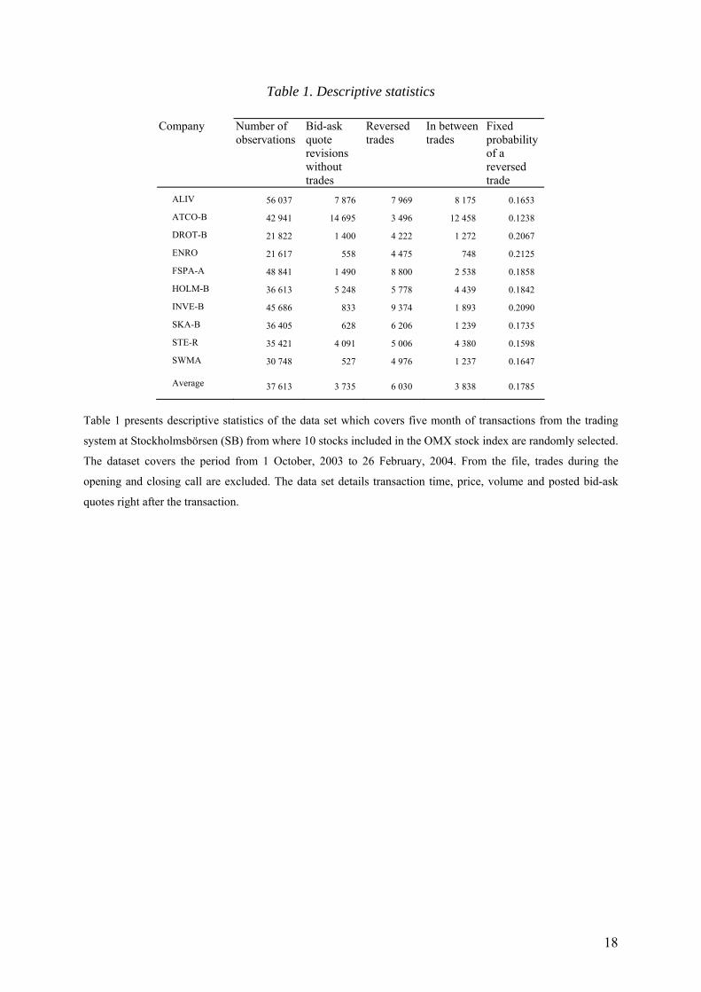
Table 1 presents descriptive statistics of the data set which covers five month of transactions from the trading

system at Stockholmsbörsen (SB) from where 10 stocks included in the OMX stock index are randomly selected.

The dataset covers the period from 1 October, 2003 to 26 February, 2004. From the file, trades during the

opening and closing call are excluded. The data set details transaction time, price, volume and posted bid-ask

quotes right after the transaction.

19

Table 2a. Fixed probabilities; adverse selection and inventory holding components

Adverse Selection, α Inventory Holding, β

Company Coefficient Std. Error Coefficient Std. Error

ALIV 0.1075 0.0089 0.2395 0.0062

ATCO-B 0.0812 0.0126 0.2697 0.0084

DROT-B 0.0737 0.0110 0.1451 0.0079

ENRO 0.0247 0.0093 0.1009 0.0066

FSPA-A 0.0258 0.0059 0.0933 0.0040

HOLM-B 0.0936 0.0103 0.1958 0.0073

INVE-B 0.0031 0.0052 0.0602 0.0037

SKA-B 0.0091 0.0052 0.0516 0.0034

STE-R 0.0635 0.0095 0.1817 0.0064

SWMA 0.0197 0.0058 0.0562 0.0038

Average 0.0502 0.0084 0.1394 0.0058

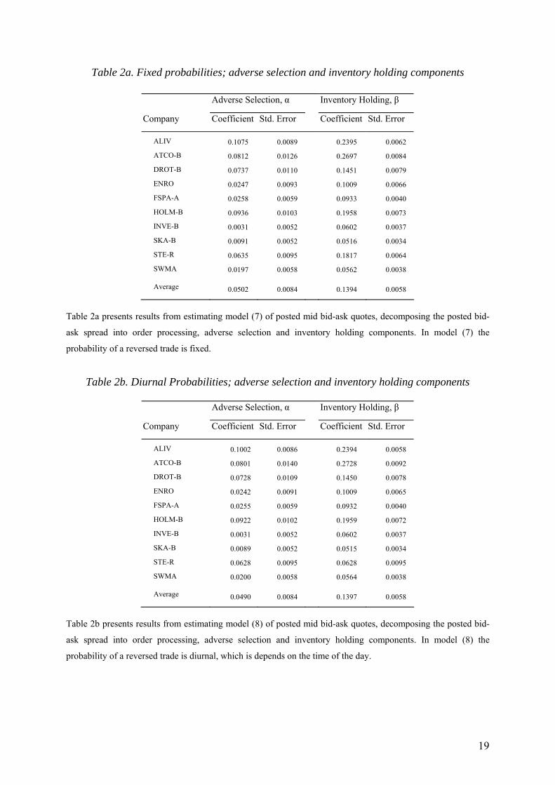
Table 2a presents results from estimating model (7) of posted mid bid-ask quotes, decomposing the posted bid-

ask spread into order processing, adverse selection and inventory holding components. In model (7) the

probability of a reversed trade is fixed.

Table 2b. Diurnal Probabilities; adverse selection and inventory holding components

Adverse Selection, α Inventory Holding, β

Company Coefficient Std. Error Coefficient Std. Error

ALIV 0.1002 0.0086 0.2394 0.0058

ATCO-B 0.0801 0.0140 0.2728 0.0092

DROT-B 0.0728 0.0109 0.1450 0.0078

ENRO 0.0242 0.0091 0.1009 0.0065

FSPA-A 0.0255 0.0059 0.0932 0.0040

HOLM-B 0.0922 0.0102 0.1959 0.0072

INVE-B 0.0031 0.0052 0.0602 0.0037

SKA-B 0.0089 0.0052 0.0515 0.0034

STE-R 0.0628 0.0095 0.0628 0.0095

SWMA 0.0200 0.0058 0.0564 0.0038

Average 0.0490 0.0084 0.1397 0.0058

Table 2b presents results from estimating model (8) of posted mid bid-ask quotes, decomposing the posted bid-

ask spread into order processing, adverse selection and inventory holding components. In model (8) the

probability of a reversed trade is diurnal, which is depends on the time of the day.

20

Table 3. Diurnal Probabilities; polynomial coefficients

Company k0 k1 k2 k3 k4

ALIV -1.136333 0.002991 -2.30E-06 5.70E-10

(0.327365) (0.000771) (5.96E-07) (1.51E-10)

ATCO-B -10.733860 0.034604 -4.10E-05 2.14E-08 -4.10E-12

(1.676133) (0.005245) (6.07E-06) (3.08E-09) (5.79E-13)

DROT-B -8.277829 0.026173 -3.00E-05 1.52E-08 -2.83E-12

(3.853978) (0.012155) (1.42E-05) (7.28E-09) (1.38E-12)

ENRO 7.057532 -0.023057 2.87E-05 1.60E-08 3.15E-12

(4.046646) (0.012709) (1.48E-05) (7.55E-9) (1.43E-12)

FSPA-A 0.128795 3.87E-05

(0.00973) (7.21E-06)

HOLM-B -13.684600 0.043056 -4.96E-05 2.51E-08 -4.72E-12

(2.732022) (0.008595) (1.00E-05) (5.12E-09) (9.71E-13)

INVE-B -6.773262 0.021311 -2.40E-05 1.18E-08 -2.14E-12

(2.737811) (0.008617) (1.00E-05) (5.14E-09) (9.77E-13)

SKA-B 0.117828 3.98E-05

(0.010922) (8.11E-06)

STE-R -5.409943 0.017674 -2.08E-05 1.08E-08 -207E-12

(2.671018) (0.008418) (9.82E-06) (5.03E-09) (9.56E-13)

SWMA 0.291947 -0.000279 1.32E-07

(0.076000) (0.000118) (4.44E-08)

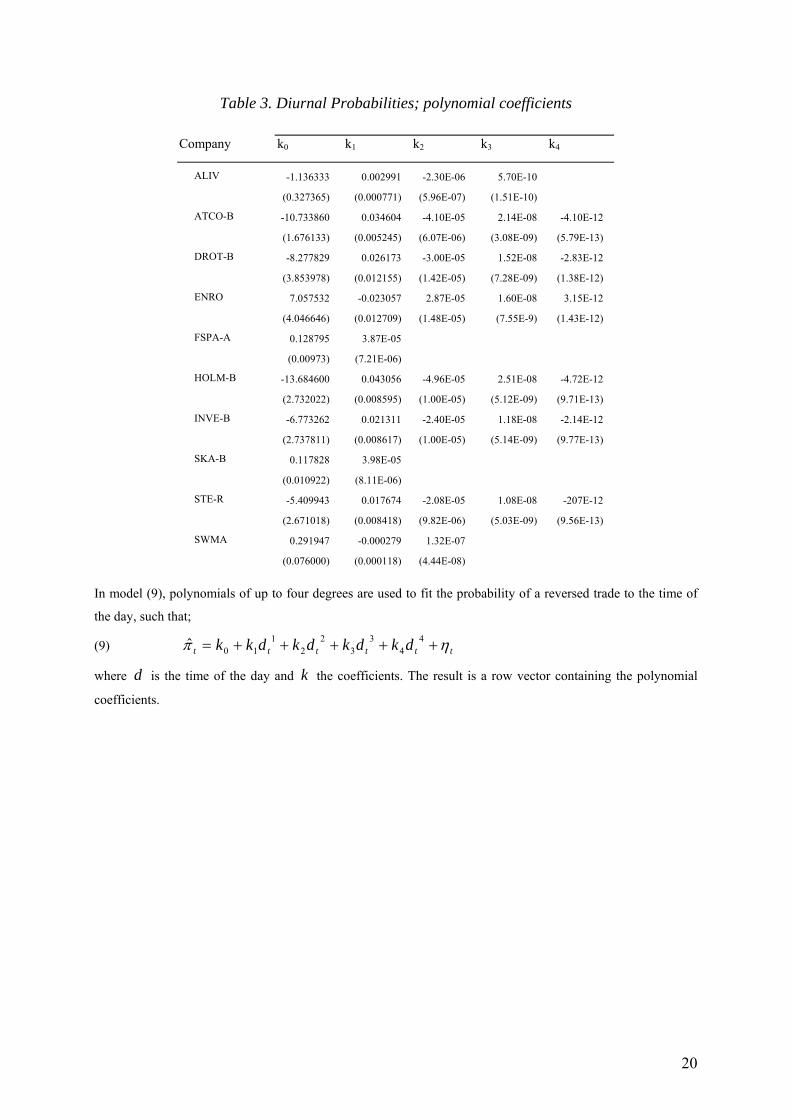
In model (9), polynomials of up to four degrees are used to fit the probability of a reversed trade to the time of

the day, such that;

(9) tttttt dkdkdkdkk ηπ +++++= 44

33

22

110ˆ

where d is the time of the day and k the coefficients. The result is a row vector containing the polynomial

coefficients.

21

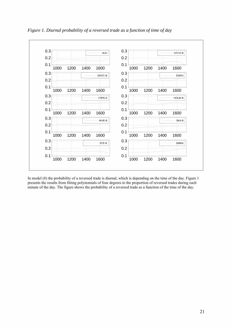
Figure 1. Diurnal probability of a reversed trade as a function of time of day

1000 1200 1400 16000.1

0.2

0.3 ALIV

1000 1200 1400 16000.1

0.2

0.3 ATCO-B

1000 1200 1400 16000.1

0.2

0.3DROT-B

1000 1200 1400 16000.1

0.2

0.3ENRO

1000 1200 1400 16000.1

0.2

0.3 FSPA-A

1000 1200 1400 16000.1

0.2

0.3 HOLM-B

1000 1200 1400 16000.1

0.2

0.3INVE-B

1000 1200 1400 16000.1

0.2

0.3SKA-B

1000 1200 1400 16000.1

0.2

0.3STE-R

1000 1200 1400 16000.1

0.2

0.3SWMA

In model (8) the probability of a reversed trade is diurnal, which is depending on the time of the day. Figure 1 presents the results from fitting polynomials of four degrees to the proportion of reversed trades during each minute of the day. The figure shows the probability of a reversed trade as a function of the time of the day.