
SHErrLoc: A Static Holistic Error Locator · ACM Reference format:...
47
18 SHErrLoc: A Static Holistic Error Locator DANFENG ZHANG, Pennsylvania State University ANDREW C. MYERS, Cornell University DIMITRIOS VYTINIOTIS and SIMON PEYTON-JONES, Microsoft Research Cambridge We introduce a general way to locate programmer mistakes that are detected by static analyses. The pro- gram analysis is expressed in a general constraint language that is powerful enough to model type checking, information flow analysis, dataflow analysis, and points-to analysis. Mistakes in program analysis result in unsatisfiable constraints. Given an unsatisfiable system of constraints, both satisfiable and unsatisfiable con- straints are analyzed to identify the program expressions most likely to be the cause of unsatisfiability. The likelihood of different error explanations is evaluated under the assumption that the programmer’s code is mostly correct, so the simplest explanations are chosen, following Bayesian principles. For analyses that rely on programmer-stated assumptions, the diagnosis also identifies assumptions likely to have been omitted. The new error diagnosis approach has been implemented as a tool called SHErrLoc, which is applied to three very different program analyses, such as type inference for a highly expressive type system implemented by the Glasgow Haskell Compiler—including type classes, Generalized Algebraic Data Types (GADTs), and type families. The effectiveness of the approach is evaluated using previously collected programs containing errors. The results show that when compared to existing compilers and other tools, SHErrLoc consistently identifies the location of programmer errors significantly more accurately, without any language-specific heuristics. CCS Concepts: • Theory of computation → Program analysis;• Software and its engineering → Software testing and debugging;• Security and privacy → Information flow control ; Additional Key Words and Phrases: Error diagnosis, static program analysis, type inference, information flow, Haskell, OCaml, Jif ACM Reference format: Danfeng Zhang, Andrew C. Myers, Dimitrios Vytiniotis, and Simon Peyton-Jones. 2017. SHErrLoc: A Static Holistic Error Locator. ACM Trans. Program. Lang. Syst. 39, 4, Article 18 (August 2017), 47 pages. https://doi.org/10.1145/3121137 1 INTRODUCTION Type systems and other static analyses help reduce the need for debugging at runtime, but sophis- ticated type systems and other program analyses can lead to terrible error messages. The difficulty This work was supported by the National Science Foundation (CCF-0964409, CCF-1566411), the Office of Naval Research (N00014-13-1-0089) and the Air Force Office of Scientific Research (FA9550-12-1-0400). Authors’ addresses: D. Zhang, the bulk of the research was done at Cornell University. He is currently affiliated with Department of Computer Science and Engineering, Pennsylvania State University, W369 Westgate Building, University Park, PA 16802, USA; email: [email protected]; A. C. Myers, Department of Computer Science, Cornell University, 428 Gates Hall, Ithaca, NY 14853, USA; email: [email protected]; D. Vytiniotis and S. Peyton-Jones, Microsoft Research Cambridge, 21 Station Road, Cambridge CB1 2FB, United Kingdom; emails: {dimitris, simonpj}@microsoft.com. Permission to make digital or hard copies of all or part of this work for personal or classroom use is granted without fee provided that copies are not made or distributed for profit or commercial advantage and that copies bear this notice and the full citation on the first page. Copyrights for components of this work owned by others than ACM must be honored. Abstracting with credit is permitted. To copy otherwise, or republish, to post on servers or to redistribute to lists, requires prior specific permission and/or a fee. Request permissions from [email protected]. © 2017 ACM 0164-0925/2017/08-ART18 $15.00 https://doi.org/10.1145/3121137 ACM Transactions on Programming Languages and Systems, Vol. 39, No. 4, Article 18. Publication date: August 2017.
-
Upload
vuongtuyen -
Category
Documents
-
view
213 -
download
0
Transcript of SHErrLoc: A Static Holistic Error Locator · ACM Reference format:...
18
SHErrLoc: A Static Holistic Error Locator
DANFENG ZHANG, Pennsylvania State University
ANDREW C. MYERS, Cornell University
DIMITRIOS VYTINIOTIS and SIMON PEYTON-JONES, Microsoft Research Cambridge
We introduce a general way to locate programmer mistakes that are detected by static analyses. The pro-
gram analysis is expressed in a general constraint language that is powerful enough to model type checking,
information flow analysis, dataflow analysis, and points-to analysis. Mistakes in program analysis result in
unsatisfiable constraints. Given an unsatisfiable system of constraints, both satisfiable and unsatisfiable con-
straints are analyzed to identify the program expressions most likely to be the cause of unsatisfiability. The
likelihood of different error explanations is evaluated under the assumption that the programmer’s code is
mostly correct, so the simplest explanations are chosen, following Bayesian principles. For analyses that rely
on programmer-stated assumptions, the diagnosis also identifies assumptions likely to have been omitted.
The new error diagnosis approach has been implemented as a tool called SHErrLoc, which is applied to three
very different program analyses, such as type inference for a highly expressive type system implemented
by the Glasgow Haskell Compiler—including type classes, Generalized Algebraic Data Types (GADTs), and
type families. The effectiveness of the approach is evaluated using previously collected programs containing
errors. The results show that when compared to existing compilers and other tools, SHErrLoc consistently
identifies the location of programmer errors significantly more accurately, without any language-specific
heuristics.
CCS Concepts: • Theory of computation → Program analysis; • Software and its engineering →
Software testing and debugging; • Security and privacy → Information flow control;
Additional Key Words and Phrases: Error diagnosis, static program analysis, type inference, information flow,
Haskell, OCaml, Jif
ACM Reference format:
Danfeng Zhang, Andrew C. Myers, Dimitrios Vytiniotis, and Simon Peyton-Jones. 2017. SHErrLoc: A Static
Holistic Error Locator. ACM Trans. Program. Lang. Syst. 39, 4, Article 18 (August 2017), 47 pages.
https://doi.org/10.1145/3121137
1 INTRODUCTION
Type systems and other static analyses help reduce the need for debugging at runtime, but sophis-ticated type systems and other program analyses can lead to terrible error messages. The difficulty
This work was supported by the National Science Foundation (CCF-0964409, CCF-1566411), the Office of Naval Research
(N00014-13-1-0089) and the Air Force Office of Scientific Research (FA9550-12-1-0400).
Authors’ addresses: D. Zhang, the bulk of the research was done at Cornell University. He is currently affiliated with
Department of Computer Science and Engineering, Pennsylvania State University, W369 Westgate Building, University
Park, PA 16802, USA; email: [email protected]; A. C. Myers, Department of Computer Science, Cornell University, 428
Gates Hall, Ithaca, NY 14853, USA; email: [email protected]; D. Vytiniotis and S. Peyton-Jones, Microsoft Research
Cambridge, 21 Station Road, Cambridge CB1 2FB, United Kingdom; emails: {dimitris, simonpj}@microsoft.com.
Permission to make digital or hard copies of all or part of this work for personal or classroom use is granted without fee
provided that copies are not made or distributed for profit or commercial advantage and that copies bear this notice and
the full citation on the first page. Copyrights for components of this work owned by others than ACM must be honored.
Abstracting with credit is permitted. To copy otherwise, or republish, to post on servers or to redistribute to lists, requires
prior specific permission and/or a fee. Request permissions from [email protected].
© 2017 ACM 0164-0925/2017/08-ART18 $15.00
https://doi.org/10.1145/3121137
ACM Transactions on Programming Languages and Systems, Vol. 39, No. 4, Article 18. Publication date: August 2017.
18:2 D. Zhang et al.
of understanding these error messages interferes with the adoption of expressive type systems andother program analyses.
When deep, non-local software properties are being checked, the analysis may detect an incon-sistency in a part of the program far from the actual error, resulting in a misleading error message.The problem is that powerful static analyses and advanced type systems reduce an otherwise-highannotation burden by drawing information from many parts of the program. However, when theanalysis detects an error, the fact that distant parts of the program influence this determinationmakes it hard to accurately attribute blame. Determining from an error message where the trueerror lies can require an unreasonably complete understanding of how the analysis works.
We are motivated to study this problem based on experience with three programming languages:ML, Haskell [35], and Jif [41], a version of Java that statically analyzes the security of informationflow within programs. The expressive type systems in all these languages lead confusing, and evenmisleading, error messages [28, 55]. Prior work has explored a variety of methods for improving er-ror reporting in each of these languages. Although these methods are usually specialized to a singlelanguage and analysis, they still frequently fail to identify the location of programmer mistakes.
In this work, we take a more general approach. The insight is that most program analyses,including type systems and type inference algorithms, can be expressed as systems of constraintsover variables. In the case of ML type inference, variables stand for types, constraints are equalitiesbetween different type expressions, and type inference succeeds when the corresponding systemof constraints is satisfiable. With a sufficiently expressive constraint language, we show that moreadvanced features in other program analyses, such as programmer assumption in Jif informationflow analysis, quantified propositions involving functions over types, used in the Glasgow HaskellCompiler (GHC), can all be modeled in a concise yet powerful constraint language, SHErrLocConstraint Language (SCL; Section 4).
SHErrLoc comes with a customized constraint language and solver1 that identifies both sat-isfiable and unsatisfiable constraint subsets via a graph representation of the constraint system(Sections 6–8). When constraints are unsatisfiable, the question is how to report the failure indi-cating an error by the programmer. The standard practice is to report the first failed constraintalong with the program point that generated it. Unfortunately, this simple approach often resultsin misleading error messages—the actual error may be far from that program point. Another ap-proach is to report all expressions that might contribute to the error (e.g., [11, 19, 52, 55]). But suchreports are often verbose and hard to understand [24].
Our insight is that when the constraint system is unsatisfiable, a more holistic approach shouldbe taken. Rather than looking at a failed constraint in isolation, the structure of the constraintsystem as a whole should be considered. The constraint system defines paths along which infor-mation propagates; both satisfiable and unsatisfiable paths can help locate the error. An expressioninvolved in many unsatisfiable paths is more likely to be erroneous; an expression that lies on manysatisfiable paths is more likely correct. This approach can be justified on Bayesian grounds, underthe assumption, captured as a prior distribution, that code is mostly correct (Section 9).
In some languages, the satisfiability of constraint systems depends on environmental assump-tions, which we call hypotheses. The same general approach can also be used to identify hypothe-ses likely to be missing: a small, weak set of hypotheses that makes constraints satisfiable is morelikely than a large, strong set.
1One downside of using a customized constraint language and solver is the SHErrLoc solver may fall out of sync with the
ones in existing compilers, such as GHC. However, this approach is still preferable for its generality, since SHErrLoc is
intended to supplement existing compilers when they fail to provide useful error messages. As long as the solvers largely
agree on constraints, SHErrLoc can provide meaningful error reports when existing compilers are unsatisfactory.
ACM Transactions on Programming Languages and Systems, Vol. 39, No. 4, Article 18. Publication date: August 2017.
SHErrLoc: A Static Holistic Error Locator 18:3
In summary, this article presents the following contributions:
(1) We define a constraint language, SCL, and its constraint graph representation that can en-code a broad range of type systems and other analyses. In particular, we show that SCL canexpress a broad range of program analyses, such as ML type inference, Jif information flowanalysis, many dataflow analyses, points-to analysis, and features of the expressive typesystem of Haskell, including type classes, Generalized Algebraic Data Types (GADTs), andtype families (Section 4 and 5).
(2) We present a novel constraint-graph-based solving technique that handles the expressiveSCL constraint language. The novel technique allows the creation of new nodes and edgesin the graph and thereby to support counterfactual reasoning about type classes, typefamilies, and their universally quantified axioms. We prove that the new algorithm alwaysterminates (Section 6–8).
(3) We develop a Bayesian model for inferring the most likely cause of program mistakesidentified in the constraint analysis. Using a Bayesian posterior distribution [18], the al-gorithm suggests program expressions that are likely errors and offers hypotheses thatthe programmer is likely to have omitted (Section 9).
(4) We evaluate the accuracy and performance of SHErrLoc on three different sets of pro-grams written in OCaml, Haskell, and Jif. As part of this evaluation, we use large sets ofprograms collected from students using OCaml and Haskell to do programming assign-ments [20, 31]. Appealingly, high-quality results do not rely on language-specific tuning(Section 10).
Contributions in Relation to Prior Versions. This article supersedes its previous conference ver-sions presented at the Proceedings of the ACM Symposium on Principles of Programming Languages
2014 (POPL’14) [58] and the Proceedings of the ACM SIGPLAN Conference on Programming Lan-
guage Design and Implementation 2015 (PLDI’15) [59] in several ways:
• It provides the syntax (Section 4.1), graph construction (Section 6), and graph saturationalgorithm (Section 7) for the complete SCL constraint language. Earlier versions have omit-ted features for simplicity: The POPL’14 article [58] lacks quantified axioms in hypothesesand functions over constraint elements, and the PLDI’15 article [59] lacks contravariant/invariant constructors, projections, and join and meet operations on constraint elements.
• It provides an end-to-end overview of the core components of SHErrLoc (Section 2.4). Theoverview includes information that is omitted in the previous versions, such as a detaileddiscussion on how constraints are generated, how the Bayesian model works, and howerrors are reported by SHErrLoc.
• It provides a running example (Section 3) to give an in-depth view of the advanced featuresof SHErrLoc. The running example is explained throughout the article.
• It formalizes the entailment rules for the SCL constraint language (Section 4.2).• It provides more details on the decentralized label model (DLM) [40] and its encoding in
the constraint language; in particular, it proves that a confidentiality/integrity policy in theDLM model is a constructor on principals with the appropriate variance (Section 5.2).
• It shows that the SCL language is expressive enough to model a nontrivial program analysis:points-to analysis (Section 5.4).
• It proves that our constraint analysis algorithm always terminates (Section 7.5).• It also proves that “redundant” graph edges provide no extra information for error localiza-
tion (Section 8.4).
ACM Transactions on Programming Languages and Systems, Vol. 39, No. 4, Article 18. Publication date: August 2017.
18:4 D. Zhang et al.
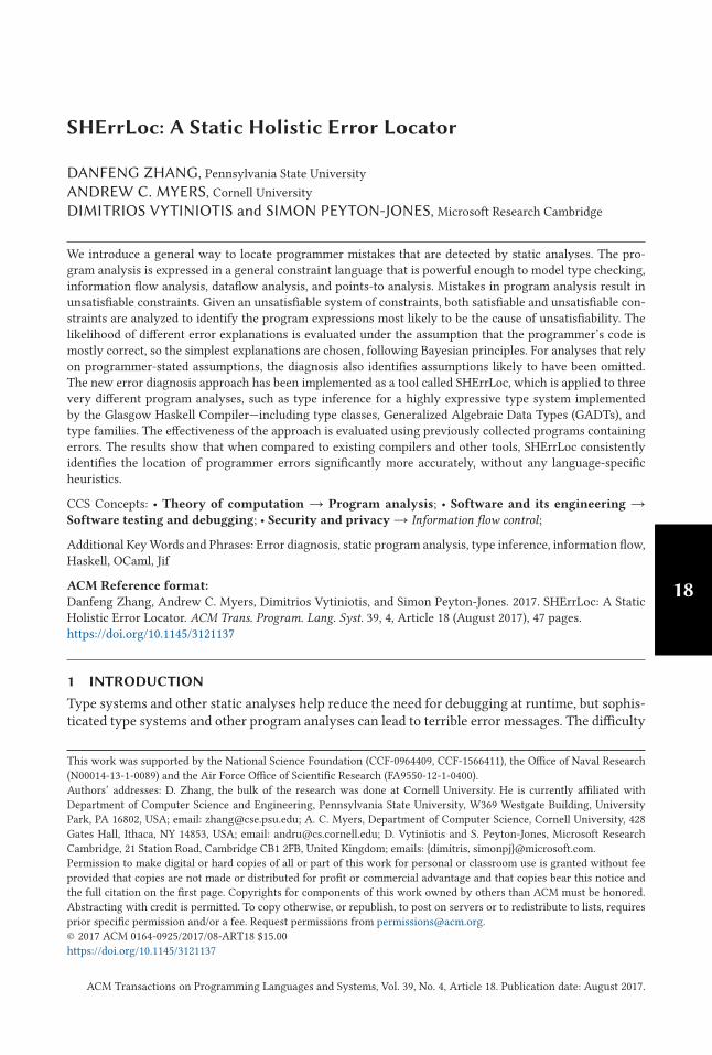
Fig. 1. OCaml example. Line 9 is blamed by OCaml compiler for a mistake at line 7.
• It describes an efficient search algorithm, based on A*, that searches for the most-likelyexplanation of program errors. The algorithm is proved to always return optimal solutions(Section 9.2).
2 APPROACH
Our general approach to diagnosing errors can be illustrated through examples from three lan-guages: ML, Haskell, and Jif.
2.1 ML Type Inference
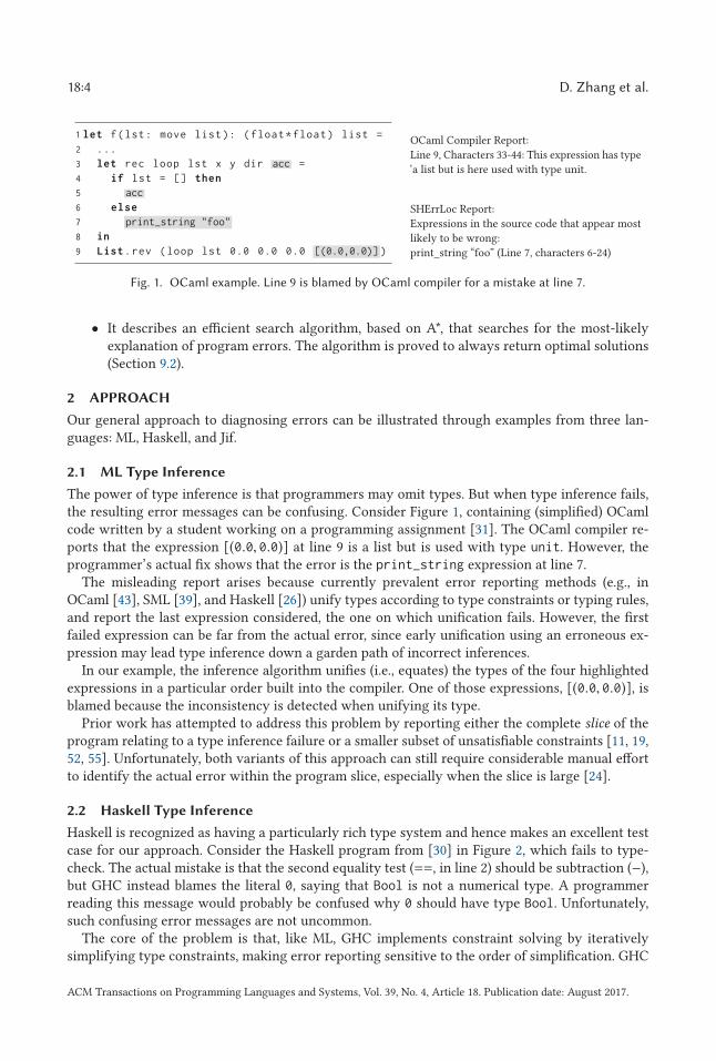
The power of type inference is that programmers may omit types. But when type inference fails,the resulting error messages can be confusing. Consider Figure 1, containing (simplified) OCamlcode written by a student working on a programming assignment [31]. The OCaml compiler re-ports that the expression [(0.0, 0.0)] at line 9 is a list but is used with type unit. However, theprogrammer’s actual fix shows that the error is the print_string expression at line 7.
The misleading report arises because currently prevalent error reporting methods (e.g., inOCaml [43], SML [39], and Haskell [26]) unify types according to type constraints or typing rules,and report the last expression considered, the one on which unification fails. However, the firstfailed expression can be far from the actual error, since early unification using an erroneous ex-pression may lead type inference down a garden path of incorrect inferences.
In our example, the inference algorithm unifies (i.e., equates) the types of the four highlightedexpressions in a particular order built into the compiler. One of those expressions, [(0.0, 0.0)], isblamed because the inconsistency is detected when unifying its type.
Prior work has attempted to address this problem by reporting either the complete slice of theprogram relating to a type inference failure or a smaller subset of unsatisfiable constraints [11, 19,52, 55]. Unfortunately, both variants of this approach can still require considerable manual effortto identify the actual error within the program slice, especially when the slice is large [24].
2.2 Haskell Type Inference
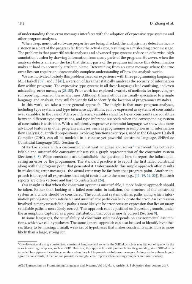
Haskell is recognized as having a particularly rich type system and hence makes an excellent testcase for our approach. Consider the Haskell program from [30] in Figure 2, which fails to type-check. The actual mistake is that the second equality test (==, in line 2) should be subtraction (−),but GHC instead blames the literal 0, saying that Bool is not a numerical type. A programmerreading this message would probably be confused why 0 should have type Bool. Unfortunately,such confusing error messages are not uncommon.
The core of the problem is that, like ML, GHC implements constraint solving by iterativelysimplifying type constraints, making error reporting sensitive to the order of simplification. GHC
ACM Transactions on Programming Languages and Systems, Vol. 39, No. 4, Article 18. Publication date: August 2017.
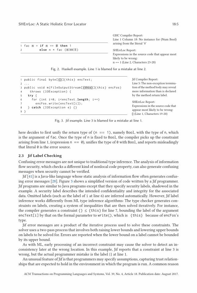
SHErrLoc: A Static Holistic Error Locator 18:5
Fig. 2. Haskell example. Line 1 is blamed for a mistake at line 2.
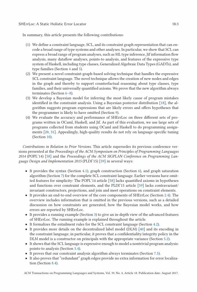
Fig. 3. Jif example. Line 3 is blamed for a mistake at line 1.
here decides to first unify the return type of (n == 1), namely Bool, with the type of n, whichis the argument of fac. Once the type of n is fixed to Bool, the compiler picks up the constraintarising from line 1, (expression n == 0), unifies the type of 0 with Bool, and reports misleadinglythat literal 0 is the error source.
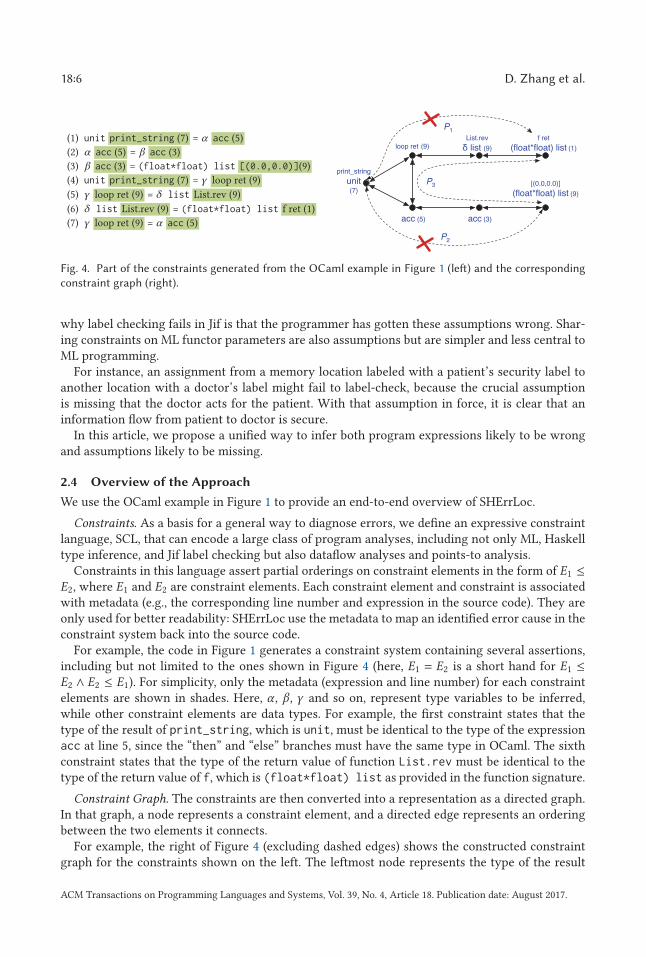
2.3 Jif Label Checking
Confusing error messages are not unique to traditional type inference. The analysis of informationflow security, which checks a different kind of nonlocal code property, can also generate confusingmessages when security cannot be verified.
Jif [41] is a Java-like language whose static analysis of information flow often generates confus-ing error messages [28]. Figure 3 shows a simplified version of code written by a Jif programmer.Jif programs are similar to Java programs except that they specify security labels, shadowed in theexample. A security label describes the intended confidentiality and integrity for the associateddata. Omitted labels (such as the label of i at line 6) are inferred automatically. However, Jif labelinference works differently from ML type inference algorithms: The type checker generates con-straints on labels, creating a system of inequalities that are then solved iteratively. For instance,the compiler generates a constraint {} ≤ {this} for line 7, bounding the label of the argumentencText[i] by that on the formal parameter to write(), which is {this} because of encFos’stype.
Jif error messages are a product of the iterative process used to solve these constraints. Thesolver uses a two-pass process that involves both raising lower bounds and lowering upper boundson labels to be solved for. Errors are reported when the lower bound on a label cannot be boundedby its upper bound.
As with ML, early processing of an incorrect constraint may cause the solver to detect an in-consistency later at the wrong location. In this example, Jif reports that a constraint at line 3 iswrong, but the actual programmer mistake is the label {} at line 1.
An unusual feature of Jif is that programmers may specify assumptions, capturing trust relation-ships that are expected to hold in the environment in which the program is run. A common reason
ACM Transactions on Programming Languages and Systems, Vol. 39, No. 4, Article 18. Publication date: August 2017.
18:6 D. Zhang et al.
Fig. 4. Part of the constraints generated from the OCaml example in Figure 1 (left) and the corresponding
constraint graph (right).
why label checking fails in Jif is that the programmer has gotten these assumptions wrong. Shar-ing constraints on ML functor parameters are also assumptions but are simpler and less central toML programming.
For instance, an assignment from a memory location labeled with a patient’s security label toanother location with a doctor’s label might fail to label-check, because the crucial assumptionis missing that the doctor acts for the patient. With that assumption in force, it is clear that aninformation flow from patient to doctor is secure.
In this article, we propose a unified way to infer both program expressions likely to be wrongand assumptions likely to be missing.
2.4 Overview of the Approach
We use the OCaml example in Figure 1 to provide an end-to-end overview of SHErrLoc.
Constraints. As a basis for a general way to diagnose errors, we define an expressive constraintlanguage, SCL, that can encode a large class of program analyses, including not only ML, Haskelltype inference, and Jif label checking but also dataflow analyses and points-to analysis.
Constraints in this language assert partial orderings on constraint elements in the form of E1 ≤E2, where E1 and E2 are constraint elements. Each constraint element and constraint is associatedwith metadata (e.g., the corresponding line number and expression in the source code). They areonly used for better readability: SHErrLoc use the metadata to map an identified error cause in theconstraint system back into the source code.
For example, the code in Figure 1 generates a constraint system containing several assertions,including but not limited to the ones shown in Figure 4 (here, E1 = E2 is a short hand for E1 ≤E2 ∧ E2 ≤ E1). For simplicity, only the metadata (expression and line number) for each constraintelements are shown in shades. Here, α , β , γ and so on, represent type variables to be inferred,while other constraint elements are data types. For example, the first constraint states that thetype of the result of print_string, which is unit, must be identical to the type of the expressionacc at line 5, since the “then” and “else” branches must have the same type in OCaml. The sixthconstraint states that the type of the return value of function List.rev must be identical to thetype of the return value of f, which is (float*float) list as provided in the function signature.
Constraint Graph. The constraints are then converted into a representation as a directed graph.In that graph, a node represents a constraint element, and a directed edge represents an orderingbetween the two elements it connects.
For example, the right of Figure 4 (excluding dashed edges) shows the constructed constraintgraph for the constraints shown on the left. The leftmost node represents the type of the result
ACM Transactions on Programming Languages and Systems, Vol. 39, No. 4, Article 18. Publication date: August 2017.
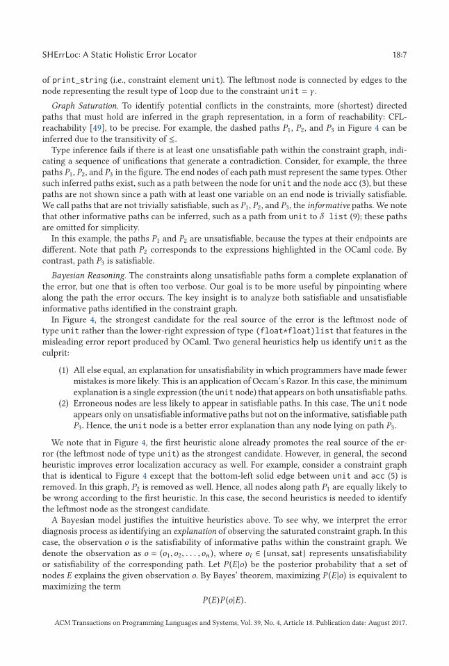
SHErrLoc: A Static Holistic Error Locator 18:7
of print_string (i.e., constraint element unit). The leftmost node is connected by edges to thenode representing the result type of loop due to the constraint unit = γ .
Graph Saturation. To identify potential conflicts in the constraints, more (shortest) directedpaths that must hold are inferred in the graph representation, in a form of reachability: CFL-reachability [49], to be precise. For example, the dashed paths P1, P2, and P3 in Figure 4 can beinferred due to the transitivity of ≤.
Type inference fails if there is at least one unsatisfiable path within the constraint graph, indi-cating a sequence of unifications that generate a contradiction. Consider, for example, the threepaths P1, P2, and P3 in the figure. The end nodes of each path must represent the same types. Othersuch inferred paths exist, such as a path between the node for unit and the node acc (3), but thesepaths are not shown since a path with at least one variable on an end node is trivially satisfiable.We call paths that are not trivially satisfiable, such as P1, P2, and P3, the informative paths. We notethat other informative paths can be inferred, such as a path from unit to δ list (9); these pathsare omitted for simplicity.
In this example, the paths P1 and P2 are unsatisfiable, because the types at their endpoints aredifferent. Note that path P2 corresponds to the expressions highlighted in the OCaml code. Bycontrast, path P3 is satisfiable.
Bayesian Reasoning. The constraints along unsatisfiable paths form a complete explanation ofthe error, but one that is often too verbose. Our goal is to be more useful by pinpointing wherealong the path the error occurs. The key insight is to analyze both satisfiable and unsatisfiableinformative paths identified in the constraint graph.
In Figure 4, the strongest candidate for the real source of the error is the leftmost node oftype unit rather than the lower-right expression of type (float*float)list that features in themisleading error report produced by OCaml. Two general heuristics help us identify unit as theculprit:
(1) All else equal, an explanation for unsatisfiability in which programmers have made fewermistakes is more likely. This is an application of Occam’s Razor. In this case, the minimumexplanation is a single expression (the unit node) that appears on both unsatisfiable paths.
(2) Erroneous nodes are less likely to appear in satisfiable paths. In this case, The unit nodeappears only on unsatisfiable informative paths but not on the informative, satisfiable pathP3. Hence, the unit node is a better error explanation than any node lying on path P3.
We note that in Figure 4, the first heuristic alone already promotes the real source of the er-ror (the leftmost node of type unit) as the strongest candidate. However, in general, the secondheuristic improves error localization accuracy as well. For example, consider a constraint graphthat is identical to Figure 4 except that the bottom-left solid edge between unit and acc (5) isremoved. In this graph, P2 is removed as well. Hence, all nodes along path P1 are equally likely tobe wrong according to the first heuristic. In this case, the second heuristics is needed to identifythe leftmost node as the strongest candidate.
A Bayesian model justifies the intuitive heuristics above. To see why, we interpret the errordiagnosis process as identifying an explanation of observing the saturated constraint graph. In thiscase, the observation o is the satisfiability of informative paths within the constraint graph. Wedenote the observation as o = (o1,o2, . . . ,on ), where oi ∈ {unsat, sat} represents unsatisfiabilityor satisfiability of the corresponding path. Let P (E |o) be the posterior probability that a set ofnodes E explains the given observation o. By Bayes’ theorem, maximizing P (E |o) is equivalent tomaximizing the term
P (E)P (o |E).
ACM Transactions on Programming Languages and Systems, Vol. 39, No. 4, Article 18. Publication date: August 2017.
18:8 D. Zhang et al.
With a couple of simplifying assumptions (Section 9.1), the most-likely explanation can be iden-tified as a set of nodes, E, such that
(1) Any unsatisfiable path uses at least one node in E, and(2) E minimizes the term C1 |E | +C2kE , where kE is the number of satisfiable paths using at
least one node in E, and C1, C2 are some tunable constants.
We note that the Bayesian model justifies the intuitive heuristics above: the explanation is likelyto contain fewer nodes (heuristic 1) and show less frequently on satisfiable edges (heuristic 2). Ap-pealingly, these two heuristics rely only on graph structure and are oblivious to the language andprogram being diagnosed. The same generic approach can therefore be applied to very differentprogram analyses.
Error Reporting. SHErrLoc uses an instance of A∗ search algorithm to identify top-ranked expla-nations according to the termC1 |E | +C2kE . Each explanation consists of one or multiple programexpressions. For example, SHErrLoc reports the only top-ranked explanation for the OCaml pro-gram in Figure 1 as follows:
Expressions in the source code that appear most likely to be wrong:print_string “foo” (Line 7, characters 6–24)
This explanation is exactly the true mistake in the program, according to the programmer’s actualerror fix.
For the programs in Figure 2 and Figure 3, the SHErrLoc reports are shown on the right of thefigures. Again, SHErrLoc correctly and precisely localizes the actual causes of the errors in thoseexamples.
3 RUNNING EXAMPLE
To explore more advanced features of SHErrLoc, we use the Haskell program in Figure 5 as arunning example for the rest of this article. This example involves a couple of sophisticated featuresin Haskell:
• Type classes introduce, in effect, relations over types, on top of ordinary unification con-straints. For example, the type of literal 0 can be any instance of the type class Num, such asInt and Float.
• Type families are functions at the level of types:
1 type instance F [a] = (Int,a)
2 f :: F [Bool] -> Bool
3 f x = snd x
In this example, it is okay to treat x as a pair although it is declared to have type F [Bool],because of the axiom describing the behavior of the type family F. (Note that in Haskell,type [Bool] represents a list of Bool’s.)
• Type signatures. Polymorphic type signatures introduce universally quantified variablesthat cannot be unified with other types [46]. Consider the following program.
1 f :: forall a. a -> (a,a)
2 f x = (True,x)
This program is ill typed, as the body of f indicates that the function is not really polymor-phic (consider applying f 42).
ACM Transactions on Programming Languages and Systems, Vol. 39, No. 4, Article 18. Publication date: August 2017.
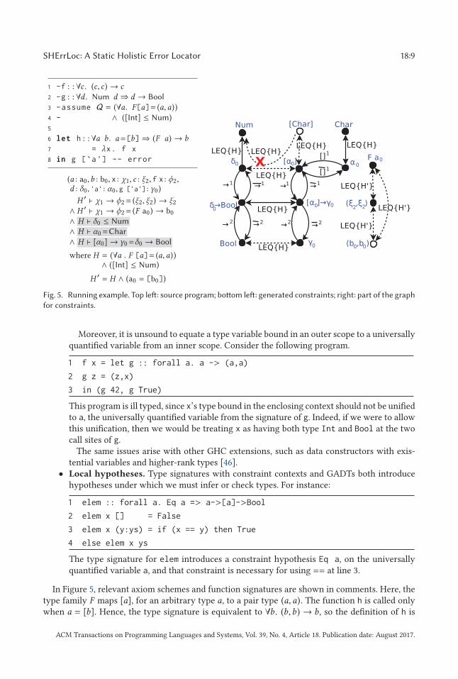
SHErrLoc: A Static Holistic Error Locator 18:9
Fig. 5. Running example. Top left: source program; bottom left: generated constraints; right: part of the graph
for constraints.
Moreover, it is unsound to equate a type variable bound in an outer scope to a universallyquantified variable from an inner scope. Consider the following program.
1 f x = let g :: forall a. a -> (a,a)
2 g z = (z,x)
3 in (g 42, g True)
This program is ill typed, since x’s type bound in the enclosing context should not be unifiedto a, the universally quantified variable from the signature of g. Indeed, if we were to allowthis unification, then we would be treating x as having both type Int and Bool at the twocall sites of g.
The same issues arise with other GHC extensions, such as data constructors with exis-tential variables and higher-rank types [46].
• Local hypotheses. Type signatures with constraint contexts and GADTs both introducehypotheses under which we must infer or check types. For instance:
1 elem :: forall a. Eq a => a->[a]->Bool
2 elem x [] = False
3 elem x (y:ys) = if (x == y) then True
4 else elem x ys
The type signature for elem introduces a constraint hypothesis Eq a, on the universallyquantified variable a, and that constraint is necessary for using == at line 3.
In Figure 5, relevant axiom schemes and function signatures are shown in comments. Here, thetype family F maps [a], for an arbitrary type a, to a pair type (a,a). The function h is called onlywhen a = [b]. Hence, the type signature is equivalent to ∀b . (b,b) → b, so the definition of h is
ACM Transactions on Programming Languages and Systems, Vol. 39, No. 4, Article 18. Publication date: August 2017.
18:10 D. Zhang et al.
Fig. 6. Syntax of SCL constraints.
well typed. On the other hand, expression (g [‘a’]) has a type error: The parameter type [Char]is not an instance of class Num, as required by the type signature of g.
The informal reasoning above corresponds to a set of constraints, shown on the bottom left ofFigure 5. From the constraints, SHErrLoc builds and saturates a constraint graph (shown on theright of Figure 5), where Bayesian reasoning is performed. We will return to the running examplewhen relevant components are introduced.
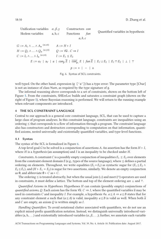
4 THE SCL CONSTRAINT LANGUAGE
Central to our approach is a general core constraint language, SCL, that can be used to capture alarge class of program analyses. In this constraint language, constraints are inequalities using anordering ≤ that corresponds to a flow of information through a program. The constraint languagealso has constructors and destructors corresponding to computation on that information, quanti-fied axioms, nested universally and existentially quantified variables, and type-level functions.
4.1 Syntax
The syntax of the SCL is formalized in Figure 6.A top-level goalG to be solved is a conjunction of assertionsA. An assertion has the form H � I ,
where H is a hypothesis (an assumption) and I is an inequality to be checked under H .
Constraints. A constraintC is a possibly empty conjunction of inequalities E1 ≤ E2 over elementsfrom the constraint element domain E (e.g., types of the source language), where ≤ defines a partialordering on elements. Throughout, we write equalities (E1=E2) as syntactic sugar for (E1 ≤E2 ∧E2 ≤E1), and (H � E1 = E2) is sugar for two assertions, similarly. We denote an empty conjunctionas ∅, and abbreviate ∅ � C as � C .
The ordering ≤ is treated abstractly, but when the usual join () and meet (�) operators are usedin constraints, it must define a lattice. The bottom and top of the element ordering are ⊥ and .
Quantified Axioms in Hypotheses. Hypotheses H can contain (possibly empty) conjunctions ofquantified axioms,Q . Each axiom has the form ∀a.C ⇒ I , where the quantified variables a may beused in constraintsC and inequality I . For example, a hypothesis ∀a. a≤A⇒ a≤B states that forany constraint element a such that (a≤A) is valid, inequality a≤B is valid as well. When both aand C are empty, an axiom Q is written simply as I .
Handling Quantifiers. To avoid notational clutter associated with quantifiers, we do not use anexplicit mixed-prefix quantification notation. Instead, we distinguish universally introduced vari-ables (a, b, . . .) and existentially introduced variables (α , β, . . .); further, we annotate each variable
ACM Transactions on Programming Languages and Systems, Vol. 39, No. 4, Article 18. Publication date: August 2017.
SHErrLoc: A Static Holistic Error Locator 18:11
with its level, a number that implicitly represents the scope in which the variable was introduced.For example, we write the formula a1=b1 � (a1, b1)=α2 to represent ∀a,b.∃α . a=b � (a, b)=α .Any assertion written using nested quantifiers can be put into prenex normal form [42] and there-fore can represented using level numbers.
Constructors and Functions over Constraint Elements. An element E may be (1) a variable; (2) an
application con_p E of a type constructor con ∈ Con, where the annotationp describes the variance
of the parameters; or (3) an application fun E of a type-function fun ∈ Fun. Constants are nullaryconstructors, with arity 0. Since constructors and functions are global, they have no levels.
The partial ordering on two applications of the same constructor is determined by the variancesp of that constructor’s arguments. For each argument, the ordering of the applications is covariantwith respect to that argument (denoted by +), contravariant with respect to that argument (−), orinvariant (±) with respect to it. For simplicity, we omit the variance p when it is irrelevant to thecontext.
The main difference between a type constructor con and a type function fun is that constructors
are injective and can be therefore be decomposed (that is, con τ = con τ ′ ⇒ τ = τ ′). Type functions
are not necessarily injective: fun τ = fun τ ′ does not entail that τ =τ ′.
Example. To model ML type inference, we can represent the type (int→ bool) as a constructorapplication fn(−,+) (int, bool), where int and bool are constants, the first argument is contravariant,
and the second argument is covariant. Its first projection fn1(fn(−,+) (int, bool)) is int.
Consider the expressions acc (line 5) and print_string (line 7) in Figure 1. These are branchesof an if statement, so one assertion is generated to enforce that they have the same type: � acc (5) ≤unit ∧ unit ≤ acc (5) .
Section 5 describes in more detail how assertions are generated for ML, Haskell, Jif, dataflowanalysis, and points-to analysis.
4.2 Validity and Satisfiability
An assertion A is satisfiable if there is a level-respecting substitution θ for A’s free unification vari-ables, such that θ[A] is valid.
A substitution θ is level respecting if the substitution is well scoped. More formally, ∀αl ∈dom(θ ), am ∈ fvs(θ[αl ]).m ≤ l . For example, an assertion a1=b1 � (a1=α2 ∧ α2=b1) is satisfiablewith substitution [α2 �→ a1]. But � α1=b2 is not satisfiable, because the substitution [α1 �→ b2]is not level respecting. The reason is that with explicit quantifiers, the latter would look like∃α∀b. � α =b and it would be ill scoped to instantiate α with b.
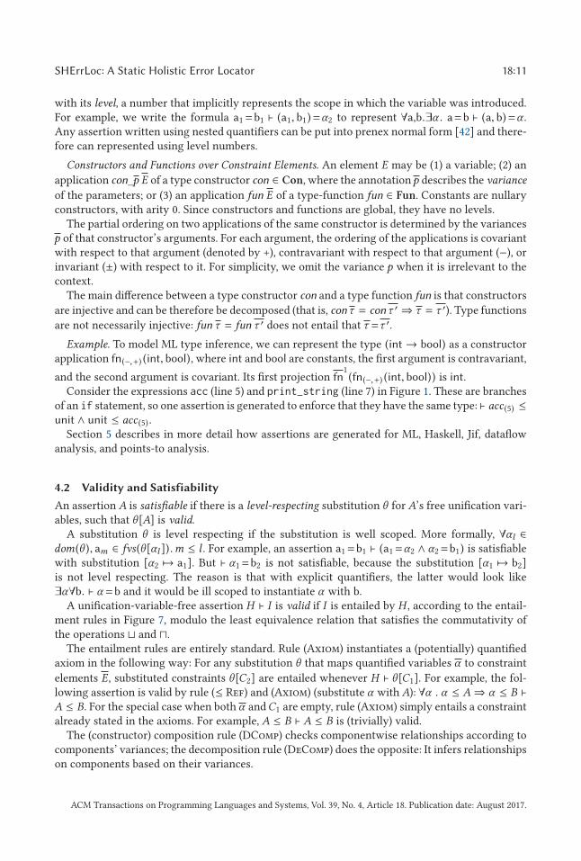
A unification-variable-free assertion H � I is valid if I is entailed by H , according to the entail-ment rules in Figure 7, modulo the least equivalence relation that satisfies the commutativity ofthe operations and �.
The entailment rules are entirely standard. Rule (Axiom) instantiates a (potentially) quantifiedaxiom in the following way: For any substitution θ that maps quantified variables α to constraint
elements E, substituted constraints θ[C2] are entailed whenever H � θ[C1]. For example, the fol-lowing assertion is valid by rule (≤ Ref) and (Axiom) (substitute α with A): ∀α . α ≤ A⇒ α ≤ B �A ≤ B. For the special case when both α andC1 are empty, rule (Axiom) simply entails a constraintalready stated in the axioms. For example, A ≤ B � A ≤ B is (trivially) valid.
The (constructor) composition rule (DComp) checks componentwise relationships according tocomponents’ variances; the decomposition rule (DeComp) does the opposite: It infers relationshipson components based on their variances.
ACM Transactions on Programming Languages and Systems, Vol. 39, No. 4, Article 18. Publication date: August 2017.
18:12 D. Zhang et al.
Fig. 7. Entailment rules.
5 EXPRESSIVENESS
The constraint language is the interface between various program analyses and SHErrLoc. To useSHErrLoc, the program analysis implementer must instrument the compiler or analysis to expressa given program analysis as a set of constraints in SCL.
As we now show, the constraint language is expressive enough to capture a variety of differentprogram analyses. Of course, the constraint language is not intended to express all program anal-yses, such as analyses that involve arithmetic. We leave incorporating a larger class of analysesinto our framework as future work.
5.1 ML Type Inference
ML type inference maps naturally into constraint solving, since typing rules can be usually beread as equality constraints on type variables. Numerous efforts have been made in this direction(e.g., [2, 19, 24, 37, 56]).
Most of these formalizations are similar, so we discuss how Damas’s Algorithm T [12] can be re-cast into our constraint language, extending the approach of Haack and Wells [19]. We follow thatapproach since it supports let-polymorphism. Further, our evaluation builds on an implementationof that approach.
For simplicity, we only discuss the subset of ML whose syntax is shown in Figure 8. However, ourimplementation does support a much larger set of language features, including match expressionsand user-defined data types.
ACM Transactions on Programming Languages and Systems, Vol. 39, No. 4, Article 18. Publication date: August 2017.
SHErrLoc: A Static Holistic Error Locator 18:13
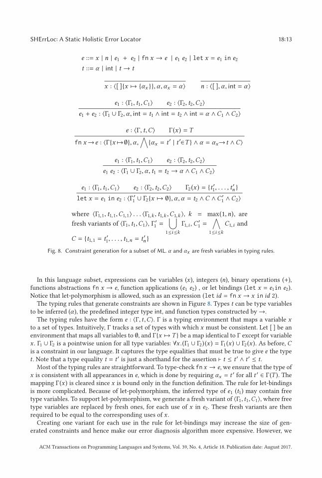
Fig. 8. Constraint generation for a subset of ML. α and αx are fresh variables in typing rules.
In this language subset, expressions can be variables (x ), integers (n), binary operations (+),functions abstractions fn x → e, function applications (e1 e2) , or let bindings (let x = e1in e2).Notice that let-polymorphism is allowed, such as an expression (let id = fn x → x in id 2).
The typing rules that generate constraints are shown in Figure 8. Types t can be type variablesto be inferred (α ), the predefined integer type int, and function types constructed by→.
The typing rules have the form e : 〈Γ, t ,C〉. Γ is a typing environment that maps a variable xto a set of types. Intuitively, Γ tracks a set of types with which x must be consistent. Let [ ] be anenvironment that maps all variables to ∅, and Γ{x �→ T } be a map identical to Γ except for variablex . Γ1 ∪ Γ2 is a pointwise union for all type variables: ∀x .(Γ1 ∪ Γ2) (x ) = Γ1 (x ) ∪ Γ2 (x ). As before, Cis a constraint in our language. It captures the type equalities that must be true to give e the typet . Note that a type equality t = t ′ is just a shorthand for the assertion � t ≤ t ′ ∧ t ′ ≤ t.
Most of the typing rules are straightforward. To type-check fn x → e, we ensure that the type ofx is consistent with all appearances in e, which is done by requiring αx = t ′ for all t ′ ∈ Γ(T ). Themapping Γ(x ) is cleared since x is bound only in the function definition. The rule for let-bindingsis more complicated. Because of let-polymorphism, the inferred type of e1 (t1) may contain freetype variables. To support let-polymorphism, we generate a fresh variant of 〈Γ1, t1,C1〉, where freetype variables are replaced by fresh ones, for each use of x in e2. These fresh variants are thenrequired to be equal to the corresponding uses of x .
Creating one variant for each use in the rule for let-bindings may increase the size of gen-erated constraints and hence make our error diagnosis algorithm more expensive. However, we
ACM Transactions on Programming Languages and Systems, Vol. 39, No. 4, Article 18. Publication date: August 2017.

18:14 D. Zhang et al.
find performance is still reasonable with this approach. One way to avoid this limitation is to addpolymorphically constrained types, as in [17]. We leave that as future work.
5.2 Information-flow Control
In information-flow control systems, information is tagged with security labels, such as “unclassi-fied” or “top secret.” Such security labels naturally form a lattice [13], and the goal of such systemsis to ensure that all information flows upward in the lattice.
To demonstrate the expressiveness of our core constraint language, we show that it can expressthe information flow checking in the Jif language [41]. To the best of our knowledge, ours is thefirst general constraint language expressive enough to model the challenging features of Jif.
Label Inference and Checking. Jif [41] statically analyzes the security of information flow withinprograms. All types are annotated with security labels drawn from the DLM [40].
Information flow is checked by the Jif compiler using constraint solving. For instance, given anassignment x := y, the compiler generates a constraint L(y) ≤ L(x ), meaning that the label of xmust be at least as restrictive as that of y.
The programmer can omit some security labels and let the compiler generate them. For instance,when the label of x is not specified, assignment x := y generates a constraint L(y) ≤ αx , where αx
is a label variable to be inferred.Hence, Jif constraints are broadly similar in structure to our general constraint language. How-
ever, some features of Jif are challenging to model.
Label Model. The basic building block of the DLM is a set of principals representing users andother authority entities. Principals are structured as a lattice with respect to a relation actsfor . Theproposition A actsfor B means A is at least as privileged as B; that is, A is at most as restricted inits activities as B.
For instance, if doctor A actsfor patient B, then doctor A is allowed to read all information thatpatient B can read. However, such relation does not grant doctor A to read any information patientC can read, unless doctor A actsfor patient C, too. The actsfor relation can be expressed by thepartial ordering ≤: For example, the relationship A actsfor B is modeled by the inequality B ≤ A.
Security policies on information are expressed as labels that mention these principals. For ex-ample, the confidentiality label {patient→ doctor} means that the principal patient permitsthe principal doctor to learn the labeled information. Principals can be used to construct integritylabels as well.
A (confidentiality) label L contains a set of principals called the owners. For each owner O , thelabel also contains a set of principals called the readers. Readers are the principals to whom ownerO is willing to release the information.
For instance, a label {o1 → r1 � r2; o2 → r2 � r3} can be read as follows: principal o1 allows prin-cipals r1 or r2 to read the tagged information, and principal o2 allows principals r2 or r3 to read.Only the principals in the effective reader set, the intersection of the readers of all owners, mayread the information.
In the presence of the actsfor relation ≤, the effective reader set readers(p,L), the set of principalsthat p believes should be allowed to read information with label L, is defined as follows:
readers(p,o → r ) � {q | if p ≤ o then(o ≤ q or r ≤ q)}.
When principal p does not trust o (o does not act for p), the effective reader set is all principals,since p does not credit the policy with any significance. In other words, p has to conservativelyassume that the information with the label o → r is not protected at all when p does not trust o.Note that though the effective reader set for p is all principals in this case, p is not allowed to read
ACM Transactions on Programming Languages and Systems, Vol. 39, No. 4, Article 18. Publication date: August 2017.
SHErrLoc: A Static Holistic Error Locator 18:15
the data if neither o ≤ p nor r ≤ p holds. The reason is that p is not in the effective reader set of o.As we formalize next, information flow is allowed only if a reader is in the effective reader sets ofall principals.
Using the definition of effective reader set, the “no more restrictive than” relation ≤ on confi-dentiality policies is formalized as:
c ≤ d ⇐⇒ ∀p. readers(p, c ) ⊇ readers(p,d ).
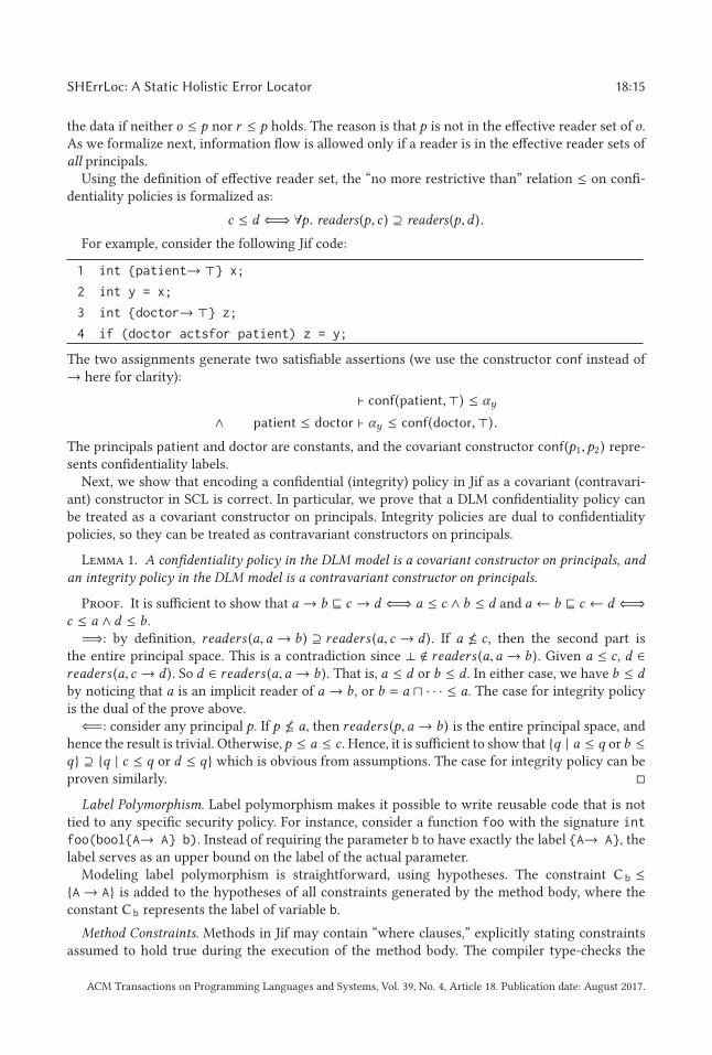
For example, consider the following Jif code:
1 int {patient→ } x;
2 int y = x;
3 int {doctor→ } z;
4 if (doctor actsfor patient) z = y;
The two assignments generate two satisfiable assertions (we use the constructor conf instead of→ here for clarity):
� conf(patient, ) ≤ αy
∧ patient ≤ doctor � αy ≤ conf(doctor, ).
The principals patient and doctor are constants, and the covariant constructor conf(p1,p2) repre-sents confidentiality labels.
Next, we show that encoding a confidential (integrity) policy in Jif as a covariant (contravari-ant) constructor in SCL is correct. In particular, we prove that a DLM confidentiality policy canbe treated as a covariant constructor on principals. Integrity policies are dual to confidentialitypolicies, so they can be treated as contravariant constructors on principals.
Lemma 1. A confidentiality policy in the DLM model is a covariant constructor on principals, and
an integrity policy in the DLM model is a contravariant constructor on principals.
Proof. It is sufficient to show that a → b � c → d ⇐⇒ a ≤ c ∧ b ≤ d and a ← b � c ← d ⇐⇒c ≤ a ∧ d ≤ b.=⇒: by definition, readers (a,a → b) ⊇ readers (a, c → d ). If a �≤ c , then the second part is
the entire principal space. This is a contradiction since ⊥ � readers (a,a → b). Given a ≤ c , d ∈readers (a, c → d ). So d ∈ readers (a,a → b). That is, a ≤ d or b ≤ d . In either case, we have b ≤ dby noticing that a is an implicit reader of a → b, or b = a � · · · ≤ a. The case for integrity policyis the dual of the prove above.⇐=: consider any principal p. If p �≤ a, then readers (p,a → b) is the entire principal space, and
hence the result is trivial. Otherwise,p ≤ a ≤ c . Hence, it is sufficient to show that {q | a ≤ q orb ≤q} ⊇ {q | c ≤ q or d ≤ q} which is obvious from assumptions. The case for integrity policy can beproven similarly. �
Label Polymorphism. Label polymorphism makes it possible to write reusable code that is nottied to any specific security policy. For instance, consider a function foo with the signature intfoo(bool{A→ A} b). Instead of requiring the parameter b to have exactly the label {A→ A}, thelabel serves as an upper bound on the label of the actual parameter.
Modeling label polymorphism is straightforward, using hypotheses. The constraint C b ≤{A→ A} is added to the hypotheses of all constraints generated by the method body, where theconstant C b represents the label of variable b.
Method Constraints. Methods in Jif may contain “where clauses,” explicitly stating constraintsassumed to hold true during the execution of the method body. The compiler type-checks the
ACM Transactions on Programming Languages and Systems, Vol. 39, No. 4, Article 18. Publication date: August 2017.
18:16 D. Zhang et al.
method body under these assumptions and ensures that the assumptions are true at all methodcall sites. In the constraint language, method constraints are modeled as hypotheses.
5.3 Dataflow Analysis
Dataflow analysis is used not only to optimize code but also to check for common errors such asuninitialized variables and unreachable code. Classic instances of dataflow analysis include reach-ing definitions, live variable analysis and constant propagation.
Aiken [1] showed how to formalize dataflow analysis algorithms as the solution of a set of con-straints with equalities over the following elements (a subclass of the more general set constraints
in [1]):
E ::= A1 | . . . | An | α | E1 ∪ E2 | E1 ∩ E2 |¬E,
where A1, . . . ,An are constants, α is a constraint variable, elements represents sets of constants,and ∪,∩,¬ are the usual set operators.
Consider live variable analysis. Let Sdef and Suse be the set of program variables that are definedand used in a statement S , and let succ (S ) be the statement executed immediately after S . Twoconstraints are generated for statement S :
Sin = Suse ∪ (Sout ∩ ¬Sdef )
Sout =⋃
X ∈succ (S )
Xin
where Sin , Sout ,Xin are constraint variables.Our constraint language is expressive enough to formalize common dataflow analyses since the
constraint language above is nearly a subset of ours: Set inclusion is a partial order, and negationcan be eliminated by preprocessing in the common case where the number of constants is finite(e.g., ¬Sdef is finite).
5.4 Points-to Analysis
Points-to analysis statically computes a set of memory locations that each pointer-valued expres-sion may point to. The analysis is widely used in optimization and other program analyses. Al-though points-to analysis is commonly used as a component of more complex analyses, such asescape analysis, the fact that a pointer-valued expression points to an unexpected location maylead to confusing analysis results.
We focus on two commonly used flow-insensitive approaches: the equality-based approach ofSteensgaard [51] and the subset-based approach of Andersen [3].
One subtlety in formalizing points-to analysis as constraint solving is that a reference can be-have both covariantly and contravariantly depending on whether a value is retrieved or set [16].Mutable reference type τ can be viewed as an abstract data type with two operations: get: unit→ τand set: τ → unit, where τ is covariant in get and contravariant in set. To reflect the get and set oper-ations of mutable references in typing rules, we follow the approach of Foster et al. [16], who use aconstructor ref (+,−) to choose the flow of information. Here, we demonstrate the expressive powerof SCL by casting the constraint generation algorithm proposed by Foster et al. [16] to equivalenttyping rules generating SCL constraints. However, the use of projections in SCL allows our typingrules to be simpler. The Andersen-style analysis for an imperative language subset is modeled by
ACM Transactions on Programming Languages and Systems, Vol. 39, No. 4, Article 18. Publication date: August 2017.
SHErrLoc: A Static Holistic Error Locator 18:17
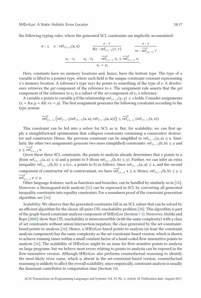
the following typing rules, where the generated SCL constraints are implicitly accumulated:
n : ⊥ x : ref (+,−) (x, x)e : τ
&e : ref (+,−) (τ ,τ )
e : τ
∗e : ref1
(+,−) τ
e1 : τ1 e2 : τ2 ref1
(+,−) τ2 ≤ ref2
(+,−) τ1
e1 = e2.
Here, constants have no memory locations and, hence, have the bottom type. The type of avariable is lifted to a pointer type, where each field is the unique constraint constant representingx ’s memory location. A reference’s type says &e points to something of the type of e . A derefer-ence retrieves the get component of the reference to e . The assignment rule asserts that the get
component of the reference to e2 is a subset of the set component of e1’s reference.A variable x points to variabley if the relationship ref (+,−) (y, y) ≤ x holds. Consider assignments
(x = &a;y = &b; ∗x = y). The first assignment generates the following constraint according to thetype system:
ref1
(+,−)
(ref (+,−) (ref (+,−) (a, a), ref (+,−) (a, a))
)≤ ref
2
(+,−) (ref (+,−) (x, x))
This constraint can be fed into a solver for SCL as is. But, for scalability, we can first ap-ply a straightforward optimization that collapses constraints containing a consecutive destruc-tor and constructor. Hence, the previous constraint can be simplified to ref (+,−) (a, a) ≤ x. Simi-larly, the other two assignments generate two more (simplified) constraints: ref (+,−) (b, b) ≤ y and
y ≤ ref2
(+,−) x.Given these three SCL constraints, the points-to analysis already determines that x points to a
(from ref (+,−) (a, a) ≤ x) and y points to b (from ref (+,−) (b, b) ≤ y). Further, we can infer an extrainequality ref (+,−) (b, b) ≤ a (i.e., a points to b) as follows. Since ref (+,−) (a, a) ≤ x, and the second
component of constructor ref is contravariant, we have ref2
(+,−) x ≤ a. Hence, ref (+,−) (b, b) ≤ y ≤ref
2
(+,−) x ≤ a.Other language features, such as functions and branches, can be handled by similarly as in [16].
Moreover, a Steensgaard-style analysis [51] can be expressed in SCL by converting all generatedinequality constraints into equality constraints. For a soundness proof of the constraint generationalgorithm, see [16].
Scalability. We observe that the generated constraints fall in an SCL subset that can be solved byan efficient algorithm for the classic all-pairs CFL-reachability problem [38]. This algorithm is partof the graph-based constraint analysis component of SHErrLoc (Section 7.1). Moreover, Melski andReps [2000] show that CFL reachability is interconvertible (with the same complexity) with a classof set constraints without union/intersection/negation, the class generated by the set-constraint-based points-to analysis [16]. Hence, a SHErrLoc-based points-to analysis (at least the constraintanalysis component) has the same complexity as the set-constraint-based version, which is shownto achieve running times within a small constant factor of a hand-coded flow-insensitive points-toanalysis [16]. The scalability of SHErrLoc might be an issue for flow-sensitive points-to analysison large programs, but we believe most errors relating to points-to analysis can be exposed in theflow-insensitive version. Although SHErrLoc also performs counterfactual reasoning to identifythe most-likely error cause, which is absent in the set-constraint-based version, counterfactualreasoning is unlikely to affect the overall scalability, since empirically, constraint analysis is usuallythe dominant contributor to computation time (Section 10).
ACM Transactions on Programming Languages and Systems, Vol. 39, No. 4, Article 18. Publication date: August 2017.
18:18 D. Zhang et al.
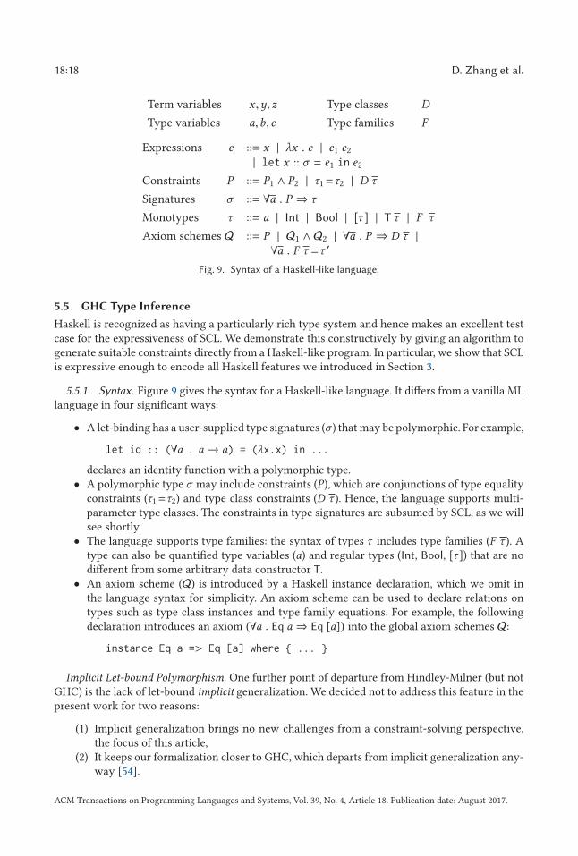
Fig. 9. Syntax of a Haskell-like language.
5.5 GHC Type Inference
Haskell is recognized as having a particularly rich type system and hence makes an excellent testcase for the expressiveness of SCL. We demonstrate this constructively by giving an algorithm togenerate suitable constraints directly from a Haskell-like program. In particular, we show that SCLis expressive enough to encode all Haskell features we introduced in Section 3.
5.5.1 Syntax. Figure 9 gives the syntax for a Haskell-like language. It differs from a vanilla MLlanguage in four significant ways:
• A let-binding has a user-supplied type signatures (σ ) that may be polymorphic. For example,
let id :: (∀a . a → a) = (λx.x) in ...
declares an identity function with a polymorphic type.• A polymorphic type σ may include constraints (P ), which are conjunctions of type equality
constraints (τ1=τ2) and type class constraints (D τ ). Hence, the language supports multi-parameter type classes. The constraints in type signatures are subsumed by SCL, as we willsee shortly.
• The language supports type families: the syntax of types τ includes type families (F τ ). Atype can also be quantified type variables (a) and regular types (Int, Bool, [τ ]) that are nodifferent from some arbitrary data constructor T.
• An axiom scheme (Q) is introduced by a Haskell instance declaration, which we omit inthe language syntax for simplicity. An axiom scheme can be used to declare relations ontypes such as type class instances and type family equations. For example, the followingdeclaration introduces an axiom (∀a . Eq a ⇒ Eq [a]) into the global axiom schemes Q:
instance Eq a => Eq [a] where { ... }
Implicit Let-bound Polymorphism. One further point of departure from Hindley-Milner (but notGHC) is the lack of let-bound implicit generalization. We decided not to address this feature in thepresent work for two reasons:
(1) Implicit generalization brings no new challenges from a constraint-solving perspective,the focus of this article,
(2) It keeps our formalization closer to GHC, which departs from implicit generalization any-way [54].
ACM Transactions on Programming Languages and Systems, Vol. 39, No. 4, Article 18. Publication date: August 2017.
SHErrLoc: A Static Holistic Error Locator 18:19
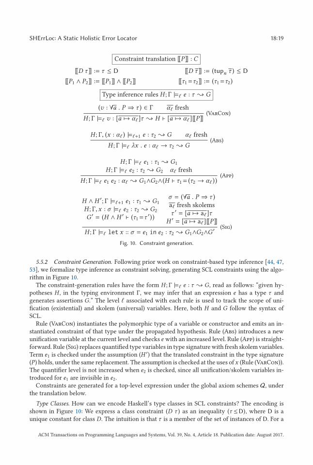
Fig. 10. Constraint generation.
5.5.2 Constraint Generation. Following prior work on constraint-based type inference [44, 47,53], we formalize type inference as constraint solving, generating SCL constraints using the algo-rithm in Figure 10.
The constraint-generation rules have the form H ; Γ |=� e : τ � G, read as follows: “given hy-potheses H , in the typing environment Γ, we may infer that an expression e has a type τ andgenerates assertions G.” The level � associated with each rule is used to track the scope of uni-fication (existential) and skolem (universal) variables. Here, both H and G follow the syntax ofSCL.
Rule (VarCon) instantiates the polymorphic type of a variable or constructor and emits an in-stantiated constraint of that type under the propagated hypothesis. Rule (Abs) introduces a newunification variable at the current level and checks e with an increased level. Rule (App) is straight-forward. Rule (Sig) replaces quantified type variables in type signature with fresh skolem variables.Term e1 is checked under the assumption (H ′) that the translated constraint in the type signature(P ) holds, under the same replacement. The assumption is checked at the uses of x (Rule (VarCon)).The quantifier level is not increased when e2 is checked, since all unification/skolem variables in-troduced for e1 are invisible in e2.
Constraints are generated for a top-level expression under the global axiom schemes Q, underthe translation below.
Type Classes. How can we encode Haskell’s type classes in SCL constraints? The encoding isshown in Figure 10: We express a class constraint (D τ ) as an inequality (τ ≤D), where D is aunique constant for class D. The intuition is that τ is a member of the set of instances of D. For a
ACM Transactions on Programming Languages and Systems, Vol. 39, No. 4, Article 18. Publication date: August 2017.
18:20 D. Zhang et al.
multi-parameter type class, the same idea applies, except that we use a constructor tupn to con-struct a single element from the parameter tuple of length n.
For example, consider a type class Mul with three parameters (the types of two operands andthe result of multiplication). The class Mul is the set of all type tuples that match the operators andresult types of a multiplication. Under the translation above, [[Mul τ1 τ2 τ3]] = (tup3 τ1 τ2 τ3 ≤ Mul).
Example. Return to the running example in Figure 5. The shaded constraints are generated forthe expression (g [‘a’]) in the following ways. Rule (VarCon) instantiates d in the signature ofg at type δ0 and generates the third constraint (recall that (Num δ0) is encoded as (δ0 ≤ Num)).Instantiate the type of character ‘a’ at type α0; hence α0=Char. Finally, using (App) on the call (g[‘a’]) generates a fresh type variable γ0 and the fifth constraint ([α0]→γ0) = (δ0→Bool). Thesethree constraints are unsatisfiable, revealing the type error for g [‘a’]. On the other hand, the firsttwo (satisfiable) constraints are generated for the implementation of function g. The hypothesesof these two constraints contain a0= [b0], added by rule (Sig).
5.6 Errors and Explanations
Recall that the goal of this work is to diagnose the cause of errors. Therefore, we are interested notjust in the satisfiability of a set of assertions but also in finding the best explanation for why theyare not satisfiable. Failures can be caused by both incorrect constraints and missing hypotheses.
Incorrect Constraints. One cause of unsatisfiability is the existence of incorrect constraints ap-pearing in the conclusions of assertions. Constraints are generated from program expressions, sothe presence of an incorrect constraint means the programmer wrote the wrong expression.
Missing Hypotheses. A second cause of unsatisfiability is the absence of constraints in the hypoth-esis. The absence of necessary hypotheses means the programmer omitted needed assumptions.
In our approach, an explanation for unsatisfiability may consist of both incorrect constraintsand missing hypotheses. To find good explanations, we proceed in two steps. The system of con-straints is first converted into a representation as a constraint graph (Section 6). This graph is thensaturated (Section 7), and paths are classified as either satisfiable or unsatisfiable (Section 8). Thegraph is then analyzed using Bayesian principles to identify the explanations most likely to becorrect (Section 9).
6 CONSTRAINT GRAPH
The SCL language has a natural graph representation that enables analyses of the system of con-straints. In particular, the satisfiability of the constraints can be tested via novel algorithms basedon context-free-language reachability in the graph.
6.1 Constraint Graph Construction in a Nutshell
A constraint graph is generated from assertions G as follows. As a running example, Figure 5shows part of the generated constraint graph for the constraints in the center column of the samefigure.
(1) For each assertion H � E1 ≤ E2, create black nodes for E1 and E2 (if they do not alreadyexist) and an edge LEQ{H } between the two. For example, nodes for δ0 → Bool and [α0]→γ0 are connected by LEQ{H }.
(2) For each constructor node con E) in the graph, create a black node for each of its immedi-ate sub-elements Ei (if they do not already exist); add a labeled constructor edge consi
from the sub-element to the node; and add a labeled decomposition edge consi in the
ACM Transactions on Programming Languages and Systems, Vol. 39, No. 4, Article 18. Publication date: August 2017.
SHErrLoc: A Static Holistic Error Locator 18:21
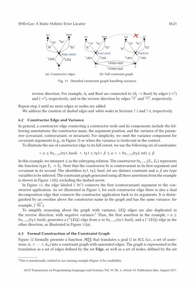
Fig. 11. Detailed constraint graph handling variance.
reverse direction. For example, δ0 and Bool are connected to (δ0 → Bool) by edges (→1)
and (→2), respectively; and in the reverse direction by edges→1 and→2, respectively.
Repeat step 2 until no more edges or nodes are added.We address the creation of dashed edges and white nodes in Sections 7.1 and 7.4, respectively.
6.2 Constructor Edge and Variance
In general, a constructor edge connecting a constructor node and its components include the fol-lowing annotations: the constructor name, the argument position, and the variance of the param-eter (covariant, contravariant, or invariant). For simplicity, we omit the variance component forcovariant arguments (e.g., in Figure 5) or when the variance is irrelevant in the context.
To illustrate the use of constructor edge to its full extent, we use the following set of constraints:
� α ≤ fn(−,+) (ty1, bool) ∧ ty1 ≤ ty2 � β ≤ α ∧ � fn(−,+) (ty2, int) ≤ β .
In this example, we interpret ≤ as the subtyping relation. The constructor fn(−,+) (E1,E2) representsthe function type E1 → E2. Note that the constructor fn is contravariant in its first argument andcovariant in its second. The identifiers ty1, ty2, bool, int are distinct constants and α , β are typevariables to be inferred. The constraint graph generated using all three assertions from the exampleis shown in Figure 11(b), excluding the dashed arrow.
In Figure 11, the edge labeled (−fn1) connects the first (contravariant) argument to the con-structor application. As we illustrated in Figure 5, for each constructor edge there is also a dualdecomposition edge that connects the constructor application back to its arguments. It is distin-guished by an overline above the constructor name in the graph and has the same variance: for
example, (−fn1).
To simplify reasoning about the graph with variance, LEQ edges are also duplicated inthe reverse direction, with negative variance.2 Thus, the first assertion in the example, � α ≤fn(−,+) (ty1, bool), generates a (+LEQ ) edge from α to fn(−,+) (ty1, bool), and a (−LEQ ) edge in theother direction, as illustrated in Figure 11(a).
6.3 Formal Construction of the Constraint Graph
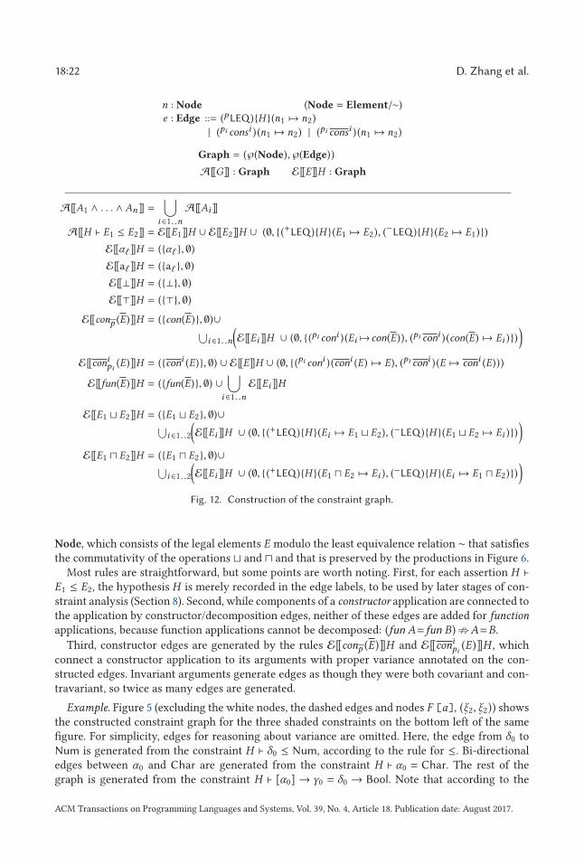
Figure 12 formally presents a function A[[]] that translates a goal G in SCL (i.e., a set of asser-tions A1 ∧ · · · ∧An ) into a constraint graph with annotated edges. The graph is represented in thetranslation as a set of edges defined by the set Edge, as well as a set of nodes, defined by the set
2This is intentionally omitted in our running example (Figure 5) for readability.
ACM Transactions on Programming Languages and Systems, Vol. 39, No. 4, Article 18. Publication date: August 2017.
18:22 D. Zhang et al.
Fig. 12. Construction of the constraint graph.
Node, which consists of the legal elements E modulo the least equivalence relation ∼ that satisfiesthe commutativity of the operations and � and that is preserved by the productions in Figure 6.
Most rules are straightforward, but some points are worth noting. First, for each assertion H �E1 ≤ E2, the hypothesis H is merely recorded in the edge labels, to be used by later stages of con-straint analysis (Section 8). Second, while components of a constructor application are connected tothe application by constructor/decomposition edges, neither of these edges are added for function
applications, because function applications cannot be decomposed: (fun A= fun B)�A=B.
Third, constructor edges are generated by the rules E[[conp (E)]]H and E[[conipi
(E)]]H , whichconnect a constructor application to its arguments with proper variance annotated on the con-structed edges. Invariant arguments generate edges as though they were both covariant and con-travariant, so twice as many edges are generated.
Example. Figure 5 (excluding the white nodes, the dashed edges and nodes F [a], (ξ2, ξ2)) showsthe constructed constraint graph for the three shaded constraints on the bottom left of the samefigure. For simplicity, edges for reasoning about variance are omitted. Here, the edge from δ0 toNum is generated from the constraint H � δ0 ≤ Num, according to the rule for ≤. Bi-directionaledges between α0 and Char are generated from the constraint H � α0 = Char. The rest of thegraph is generated from the constraint H � [α0]→ γ0 = δ0 → Bool. Note that according to the
ACM Transactions on Programming Languages and Systems, Vol. 39, No. 4, Article 18. Publication date: August 2017.
SHErrLoc: A Static Holistic Error Locator 18:23
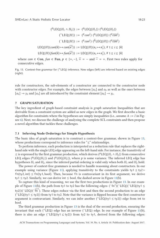
Fig. 13. Context-free grammar for (+LEQ ) inference. New edges (left) are inferred based on existing edges
(right).
rule for constructors, the sub-elements of a constructor are connected to the constructor nodewith constructor edges. For example, the edges between [α0] and α0 as well as the ones between[α0]→ γ0 and [α0] are all introduced by the constraint element [α0]→ γ0.
7 GRAPH SATURATION
The key ingredient of graph-based constraint analysis is graph saturation: Inequalities that arederivable from a constraint system are added as new edges in the graph. We first describe a basicalgorithm for constraints where the hypotheses are simply inequalities (i.e., assume A ::= I in Fig-ure 6). Next, we discuss the challenge of analyzing the complete SCL constraints and then proposea novel algorithm that tackles these challenges.
7.1 Inferring Node Orderings for Simple Hypothesis
The basic idea of graph saturation is to construct a context-free grammar, shown in Figure 13,whose productions correspond to inference rules for “≤” relationships.
To perform inference, each production is interpreted as a reduction rule that replaces the right-hand side with the single LEQ edge appearing on the left-hand side. For instance, the transitivity of≤ is expressed by the first grammar production, which derives (pLEQ{H1 ∧ H2}) from consecutiveLEQ edges (pLEQ{H1}) and (pLEQ{H2}), where p is some variance. The inferred LEQ edge hashypotheses H1 and H2, since the inferred partial ordering is valid only when both H1 and H2 hold.
The power of context-free grammars is needed to handle reasoning about constructors. In ourexample using variance (Figure 11), applying transitivity to the constraints yields ty1 ≤ ty2 �fn(ty2, int) ≤ fn(ty1, bool). Then, because fn is contravariant in its first argument, we derivety1 ≤ ty2. Similarly, we can derive int ≤ bool, the dashed arrow in Figure 11(b).
To capture this kind of reasoning, we use the first two productions in Figure 13. In our exam-ple of Figure 11(b), the path from ty1 to ty2 has the following edges: (−fn1) (−LEQ ) (−LEQ{ty1 ≤ty2}) (−LEQ ) (−fn
1). These edges reduce via the first and then the second production to an edge
(+LEQ{ty1 ≤ ty2}) from ty1 to ty2. Note that the variance is flipped because the first constructorargument is contravariant. Similarly, we can infer another (+LEQ{ty1 ≤ ty2}) edge from int tobool.
The third grammar production in Figure 13 is the dual of the second production, ensuring theinvariant that each (+LEQ ) edge has an inverse (−LEQ ) edge. In our example of Figure 11(b),there is also an edge (−LEQ{ty1 ≤ ty2}) from ty2 to ty1, derived from the following edges:
ACM Transactions on Programming Languages and Systems, Vol. 39, No. 4, Article 18. Publication date: August 2017.
18:24 D. Zhang et al.
(−fn1) (+LEQ ) (+LEQ{ty1 ≤ ty2}) (+LEQ ) (−fn1). These edges reduce via the first and then the third
production to an edge (−LEQ{ty1 ≤ ty2}) from ty2 to ty1.The last rule applies for function applications, reflecting the entailment rule (FComp) in Figure 7.Computing all inferable (+LEQ ) edges according to the context-free grammar in Figure 13 is an
instance of context-free-language reachability, which is well studied in the literature [6, 38] and hasbeen used for a number of program-analysis applications [49]. We adapt the dynamic programmingalgorithm of Barrett et al. [6] to find shortest (+LEQ ) paths. We call such paths supporting paths
since the hypotheses along these paths justify the inferred (+LEQ ) edges. We extend this algorithmto also handle join and meet nodes.
Take join nodes, for instance (meet is handled dually). The rule (Join2) in Figure 7 is alreadyhandled when we construct edges for join elements (Figure 12).
To handle the rule (Join1), we use the following procedure when a new edge (+LEQ ){H }(n1 �→n2) is processed: For each join element E where n1 is an argument of the operator, we add anedge from E to n2 if all arguments of the operator have a (+LEQ ) edge to n2.
7.2 Limitations of Pure CFL-reachability Analysis
However, graph saturation as described so far is insufficient to handle the full SCL language. Wecan see this by considering the constraint graph of the running example, in Figure 5. Excludingthe white nodes and the edges leading to and from them, this graph is fully saturated accord-ing to the rules in Figure 13. For example, the dashed edges between δ0 and [α0] can be derivedby the second production. However, a crucial inequality (edge) is missing in the saturated graph:([Char] ≤ Num), which can be derived from the shaded constraints in Figure 5. Since this inequal-ity reveals an error in the program being analyzed (that [Char] is not an instance of class Num),failure to identify it means an error is missed. Moreover, the edges between (ξ2, ξ2) and (F a0) aremistakenly judged as unsatisfiable, as we explain in Section 8.1.
7.3 Expanding the Graph
The key insight for fixing the aforementioned problems is to expand the constraint graph duringgraph saturation. Informally, nodes are added to the constraint graph so the fourth and fifth rulesin Figure 13 can be applied.
The (full) constraint graph in Figure 5 is part of the final constraint graph after running ourcomplete algorithm. The algorithm expands the original constraint graph with a new node [Char].Then, the dashed edge from [Char] to [α0] is added by the fourth production in Figure 13 and thenthe dashed edge from [Char] to Num by the first production. Therefore, the unsatisfiable inequality([Char] ≤ Num) is correctly identified by the complete algorithm. Moreover, the same mechanismdetermines that (F a0)= (b0, b0) can be entailed from hypothesis H ′, as we explain in Section 8.Hence, edges from and to (F a0) are correctly classified as satisfiable.
The key challenge for the expansion algorithm is to explore useful nodes without creating thepossibility of nontermination. For example, starting from α0=Char, a naive expansion algorithmbased on the insight above might apply the list constructor to add nodes [α0], [Char], [[α0]],[[Char]] and so on, infinitely.
7.4 The Complete Algorithm
To ensure termination, the algorithm distinguishes two kinds of graph nodes: black nodes are con-structed directly from the system of constraints (i.e., nodes added by the rules in Figure 12); white
nodes are added during graph expansion.
ACM Transactions on Programming Languages and Systems, Vol. 39, No. 4, Article 18. Publication date: August 2017.
SHErrLoc: A Static Holistic Error Locator 18:25
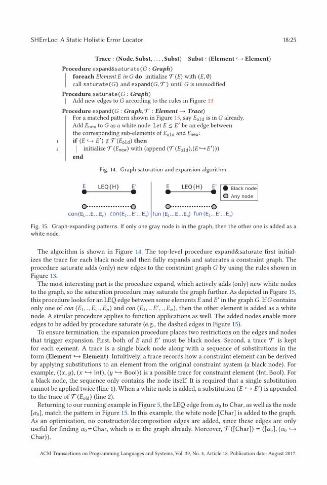
Fig. 14. Graph saturation and expansion algorithm.
Fig. 15. Graph-expanding patterns. If only one gray node is in the graph, then the other one is added as a
white node.
The algorithm is shown in Figure 14. The top-level procedure expand&saturate first initial-izes the trace for each black node and then fully expands and saturates a constraint graph. Theprocedure saturate adds (only) new edges to the constraint graph G by using the rules shown inFigure 13.
The most interesting part is the procedure expand, which actively adds (only) new white nodesto the graph, so the saturation procedure may saturate the graph further. As depicted in Figure 15,this procedure looks for an LEQ edge between some elements E and E ′ in the graphG. IfG containsonly one of con (E1, .,E, .,En ) and con (E1, .,E
′, .,En ), then the other element is added as a whitenode. A similar procedure applies to function applications as well. The added nodes enable moreedges to be added by procedure saturate (e.g., the dashed edges in Figure 15).
To ensure termination, the expansion procedure places two restrictions on the edges and nodesthat trigger expansion. First, both of E and E ′ must be black nodes. Second, a trace T is keptfor each element. A trace is a single black node along with a sequence of substitutions in theform (Element ↪→ Element). Intuitively, a trace records how a constraint element can be derivedby applying substitutions to an element from the original constraint system (a black node). Forexample, ((x ,y), (x ↪→ Int), (y ↪→ Bool)) is a possible trace for constraint element (Int,Bool). Fora black node, the sequence only contains the node itself. It is required that a single substitutioncannot be applied twice (line 1). When a white node is added, a substitution (E ↪→ E ′) is appendedto the trace of T (Eold) (line 2).
Returning to our running example in Figure 5, the LEQ edge from α0 to Char, as well as the node[α0], match the pattern in Figure 15. In this example, the white node [Char] is added to the graph.As an optimization, no constructor/decomposition edges are added, since these edges are onlyuseful for finding α0=Char, which is in the graph already. Moreover, T ([Char]) = ([α0], (α0 ↪→Char)).
ACM Transactions on Programming Languages and Systems, Vol. 39, No. 4, Article 18. Publication date: August 2017.
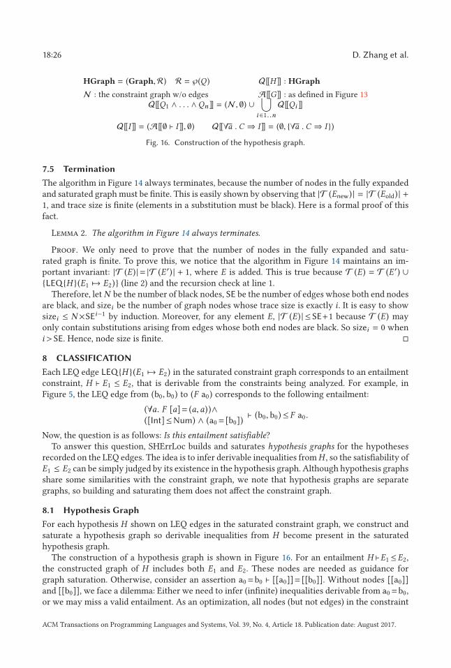
18:26 D. Zhang et al.
Fig. 16. Construction of the hypothesis graph.
7.5 Termination
The algorithm in Figure 14 always terminates, because the number of nodes in the fully expandedand saturated graph must be finite. This is easily shown by observing that |T (Enew) | = |T (Eold) | +1, and trace size is finite (elements in a substitution must be black). Here is a formal proof of thisfact.
Lemma 2. The algorithm in Figure 14 always terminates.
Proof. We only need to prove that the number of nodes in the fully expanded and satu-rated graph is finite. To prove this, we notice that the algorithm in Figure 14 maintains an im-portant invariant: |T (E) |= |T (E ′) | + 1, where E is added. This is true because T (E) = T (E ′) ∪{LEQ{H }(E1 �→ E2)} (line 2) and the recursion check at line 1.
Therefore, let N be the number of black nodes, SE be the number of edges whose both end nodesare black, and sizei be the number of graph nodes whose trace size is exactly i . It is easy to showsizei ≤ N ×SEi−1 by induction. Moreover, for any element E, |T (E) | ≤SE+1 because T (E) mayonly contain substitutions arising from edges whose both end nodes are black. So sizei = 0 wheni >SE. Hence, node size is finite. �
8 CLASSIFICATION
Each LEQ edge LEQ{H }(E1 �→ E2) in the saturated constraint graph corresponds to an entailmentconstraint, H � E1 ≤ E2, that is derivable from the constraints being analyzed. For example, inFigure 5, the LEQ edge from (b0, b0) to (F a0) corresponds to the following entailment:
(∀a. F [a]= (a,a))∧([Int]≤Num) ∧ (a0= [b0])
� (b0, b0)≤ F a0.
Now, the question is as follows: Is this entailment satisfiable?To answer this question, SHErrLoc builds and saturates hypothesis graphs for the hypotheses
recorded on the LEQ edges. The idea is to infer derivable inequalities fromH , so the satisfiability ofE1 ≤ E2 can be simply judged by its existence in the hypothesis graph. Although hypothesis graphsshare some similarities with the constraint graph, we note that hypothesis graphs are separategraphs, so building and saturating them does not affect the constraint graph.
8.1 Hypothesis Graph
For each hypothesis H shown on LEQ edges in the saturated constraint graph, we construct andsaturate a hypothesis graph so derivable inequalities from H become present in the saturatedhypothesis graph.
The construction of a hypothesis graph is shown in Figure 16. For an entailment H �E1 ≤E2,the constructed graph of H includes both E1 and E2. These nodes are needed as guidance forgraph saturation. Otherwise, consider an assertion a0=b0 � [[a0]]= [[b0]]. Without nodes [[a0]]and [[b0]], we face a dilemma: Either we need to infer (infinite) inequalities derivable from a0=b0,or we may miss a valid entailment. As an optimization, all nodes (but not edges) in the constraint
ACM Transactions on Programming Languages and Systems, Vol. 39, No. 4, Article 18. Publication date: August 2017.
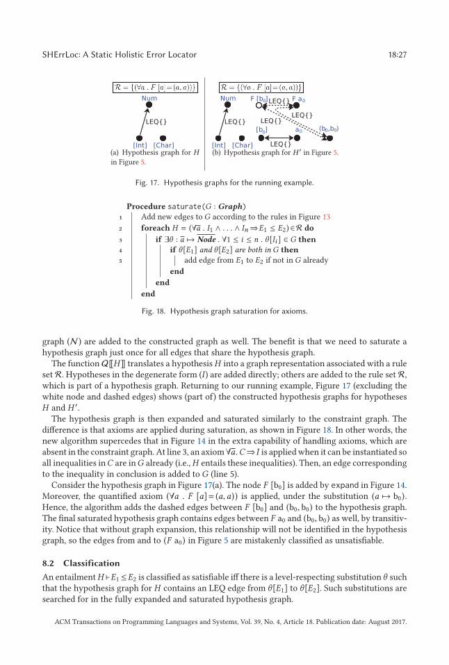
SHErrLoc: A Static Holistic Error Locator 18:27
Fig. 17. Hypothesis graphs for the running example.
Fig. 18. Hypothesis graph saturation for axioms.
graph (N ) are added to the constructed graph as well. The benefit is that we need to saturate ahypothesis graph just once for all edges that share the hypothesis graph.
The function Q[[H ]] translates a hypothesisH into a graph representation associated with a ruleset R. Hypotheses in the degenerate form (I ) are added directly; others are added to the rule set R,which is part of a hypothesis graph. Returning to our running example, Figure 17 (excluding thewhite node and dashed edges) shows (part of) the constructed hypothesis graphs for hypothesesH and H ′.
The hypothesis graph is then expanded and saturated similarly to the constraint graph. Thedifference is that axioms are applied during saturation, as shown in Figure 18. In other words, thenew algorithm supercedes that in Figure 14 in the extra capability of handling axioms, which areabsent in the constraint graph. At line 3, an axiom∀a.C⇒ I is applied when it can be instantiated soall inequalities inC are inG already (i.e.,H entails these inequalities). Then, an edge correspondingto the inequality in conclusion is added to G (line 5).
Consider the hypothesis graph in Figure 17(a). The node F [b0] is added by expand in Figure 14.Moreover, the quantified axiom (∀a . F [a]= (a,a)) is applied, under the substitution (a �→ b0).Hence, the algorithm adds the dashed edges between F [b0] and (b0, b0) to the hypothesis graph.The final saturated hypothesis graph contains edges between F a0 and (b0, b0) as well, by transitiv-ity. Notice that without graph expansion, this relationship will not be identified in the hypothesisgraph, so the edges from and to (F a0) in Figure 5 are mistakenly classified as unsatisfiable.
8.2 Classification
An entailmentH �E1 ≤E2 is classified as satisfiable iff there is a level-respecting substitution θ suchthat the hypothesis graph for H contains an LEQ edge from θ[E1] to θ[E2]. Such substitutions aresearched for in the fully expanded and saturated hypothesis graph.
ACM Transactions on Programming Languages and Systems, Vol. 39, No. 4, Article 18. Publication date: August 2017.
18:28 D. Zhang et al.
Returning to the running example in Figure 5, our algorithm correctly classifies the LEQ edgesbetween (b0, b0) and (F a0) as satisfiable, since the corresponding edges are in Figure 17(a). Ouralgorithm correctly classifies LEQ edges between (ξ2, ξ2) and (F a0) as satisfiable as well, withsubstitution ξ2 �→ b0. On the other hand, the LEQ edge from [Char] to Num is (correctly) judgedas unsatisfiable, since the inequality is not present in the fully expanded and saturated hypothesisgraph for H .
To see why the level-respecting substitution requirement is needed, consider the following ex-ample, adapted slightly from the introduction:
(λx. let g::(∀a . a → (a,a)) =
λy. (x, y) in ...)
This program generates an assertion ∅ � (β2 → (α0, β2))= (a1 → (a1, a1)), which requires thatthe inferred type for the implementation of g be equivalent to its signature. The final constraintgraph for the assertion contains two LEQ edges between nodes α0 and a1. These edges are correctlyclassified as unsatisfiable, since the only substitution candidate, α0 �→ a1, is not level respecting.
If the signature of g is (∀a . a= Int⇒a→ (a,a)), then the program is well typed, since the pa-rameter of g must be Int. This program generates the same assertion as the previous example butwith a hypothesis a1= Int. This assertion is correctly classified as satisfiable via a level-respectingsubstitution α0 �→ Int.
8.3 Informative Paths
When either end node of a satisfiable (+LEQ ) edge is a unification variable, its satisfiability is trivialand hence not informative for error diagnosis. Moreover, when either end node of an (+LEQ ) edgeis a (�) node where at least one argument of (�) is a variable, the edge is trivially satisfiable,too. For simplicity, we ignore such edges and refer subsequently only to informative (+LEQ ) edges.
When the partial ordering on the end nodes of a path is invalid, we say that the path is end-
to-end unsatisfiable. End-to-end unsatisfiable paths are helpful because the constraints along thepath explain why the inconsistency occurs.
Also useful for error diagnosis is the set of satisfiable paths: paths where there is a valid partialordering on any two nodes on the path for which a (+LEQ ) relationship can be inferred.
Any remaining paths are ignored in our error diagnosis algorithm, since by definition they mustcontain at least one end-to-end unsatisfiable subpath. For brevity, we subsequently use the termunsatisfiable path to mean a path that is end-to-end unsatisfiable.
8.4 Redundant Edges
The introduction of white nodes introduces redundant edges, whose satisfiability is determined byother edges in the graph. Consider Figure 5, the satisfiability of the edge between [α0] and [Char]merely repeats the edge between α0 and Char; the fact that end-nodes can be decomposed is alsouninformative because white nodes are constructed this way. In other words, this edge providesneither positive nor negative evidence that the constraints it captures are correct. It is redundant.We can soundly capture a large class of redundant edges:
Definition 1. An edge is redundant if
(1) both end-nodes are constructor applications of the same constructor, and at least one nodeis white; or
(2) both end-nodes are function applications to the same function, and for each simple edgealong this edge, at least one of its end-nodes is white.
Otherwise, an edge is non-redundant.
ACM Transactions on Programming Languages and Systems, Vol. 39, No. 4, Article 18. Publication date: August 2017.
SHErrLoc: A Static Holistic Error Locator 18:29
The following lemma shows that if an edge is redundant according to the previous definitionthen it does not add any positive or negative information in the graph—it is equivalent to someother set of non-redundant edges.
Lemma 3. For any redundant edge from E1 to E2, there exist non-redundant edges say Pi from Ei1
to Ei2, so E11 ≤ E12 ∧ · · · ∧ En1 ≤ En2 ⇔ E1 ≤ E2.
We first prove some auxiliary results.
Lemma 4 (Edge Simulation). For any single edge LEQ (E �→ E ′) in a fully saturated and expanded
graph G. If at least one node is white, and
(1) E = con τ and E ′ = con τ ′ for some constructor con, or
(2) E = fun τ and E ′ = fun τ ′ for some function fun,
then for any pair of corresponding parameters τi and τ ′i , either τi = τ′i , or there is an edge LEQ (τi �→
τ ′i ) in G.
Proof. Assume E is a white node without losing generality. By construction, E ∈ E ′[E1/E2] forsome elements E1 and E2.
For any pair of corresponding parameters τi and τ ′i , the interesting case is when τi � τ ′i . As-sume T (E) = (E0, s1, s2, . . . , sn ), where si ’s are substitutions. Since component substitution doesnot change the top-level structure, the black node E0 must have the form con τ0 (or fun τ0). Byconstruction, τ0i is a black node inG. Hence, the algorithm also adds τi by applying the same sub-stitutions on τ0i , as well as τ ′i by applying one more substitution τ0i [E1/E2]. LEQ (τi �→ τ ′i ) is alsoadded by saturation rules. �
Lemma 5 (Path Simulation-Cons). For any LEQ path from E1 to E2 in a fully saturated and
expanded graph G, where E1 = con τ1 and E2 = con τ2 for some constructor con. If at least one end
node is white, then for any pair of corresponding parameters τi and τ ′i , either τi = τ′i , or there is a path
from τi to τ ′i in G.
Proof. We prove by induction on the path length. The base case (length=1) is trivial byLemma 4.
Assume the conclusion holds for any path whose length ≤ k . Consider a path with length k + 1.Without losing generality, we assume E1 is a white node.
Since a white node only connects elements with same top-level constructor, the path from E1
to E2 has the form: con τ1 − con τ0 − con τ2 for some τ0. Result is true by Lemma 4 and inductionhypothesis unless both con τ0 and con τ2 are black nodes.
When both con τ0 and con τ2 are black, all of their parameters are black by graph construction.Moreover, there is a path on each pair (τ0i ,τi2) by the second production in Figure 13. ByLemma 4, there is an edge connecting τi1 and τ0i . Therefore, there is a path from τi1 to τi2 if theyare different. �
Lemma 6 (Path Simulation-Funs). For any LEQ path from E1 to E2 in a fully saturated and
expanded graphG where E1 = fun τ1 and E2 = fun τ2 for some function fun. If for any edge along the
path, at least one end node is white, then for any pair of corresponding parameters τi and τ ′i , either
τi = τ′i or there is a path from τi to τ ′i in G.
Proof. We prove by induction on the path length. The base case (length=1) is trivial byLemma 4.
ACM Transactions on Programming Languages and Systems, Vol. 39, No. 4, Article 18. Publication date: August 2017.
18:30 D. Zhang et al.
Assume the conclusion holds for any path whose length ≤ k . Consider a path with length k + 1.By assumption, every edge has at least one white node. Since a white node only connects ele-
ments with same top-level functions, the path from E1 to E2 has the form: fun τ1 − fun τ ′ − fun τ2
for some τ ′. Result is true by Lemma 4 and induction hypothesis. �
Proof of Lemma 3. For any redundant path from E1 to E2, there exist non-redundant paths inG, say, Pi from Ei1 to Ei2, so E11 ≤ E12 ∧ · · · ∧ En1 ≤ En2 ⇔ E1 ≤ E2.
Proof. We consider constructors and functions separately.
(1) When E1 = con τ1 and E2 = con τ2 for some constructor con.We construct the desired set of non-redundant paths, say,P, as follows. For each param-
eter pair τ1i and τ2i , either τ1i = τ2i or there is a path from τ1i to τ2i in G. We add nothingto P if τ1i = τ2i . Otherwise, we add the path to P if it is non-redundant. If the path is re-dundant, then we recursively add all non-redundant paths that determines τ1i ≤ τ2i to P.Easy-to-check P has the desired property, and the recursion terminates since all elementsare finite.
(2) When E1 = fun τ1 and E2 = fun τ2 for some constructor fun.Similarly to the case above, except we use Lemma 6 instead of Lemma 5 in the proof. �
Since redundant edges provides neither positive nor negative evidence for error explanation,for brevity, we subsequently use the term path to mean a path that is non-redundant.
9 BAYESIAN MODEL FOR RANKING EXPLANATIONS
The observed symptom of errors is a fully analyzed constraint graph (Section 8), in which allinformative LEQ edges are classified as satisfiable or unsatisfiable. For simplicity, in what follows,we write “edge” to mean “informative and non-redundant edge.”
Although the information along unsatisfiable paths already captures why a goal is unsat-isfiable, reporting all constraints along a path may give more information than the program-mer can digest. Our approach is to use Bayesian reasoning to identify programmer errors moreprecisely.
9.1 A Bayesian Interpretation
The cause of errors can be wrong constraints, missing hypotheses, or both. To keep our diagnosticmethod as general as possible, we avoid building in domain-specific knowledge about mistakesprogrammers tend to make. However, the framework does permit adding such knowledge in astraightforward way.
The language-level entity about which errors are reported can be specific to the language.OCaml reports typing errors in expressions, whereas Jif reports errors in information-flow con-straints. To make our diagnosis approach general, we treat entities as an abstract set Ω and assumea mapping Φ from entities to constraints. We assume a prior distribution on entities PΩ , definingthe probability that an entity is wrong. Similarly, we assume a prior distribution PΨ on hypothesesΨ, defining the probability that a hypothesis is missing.
Given entities E ⊆ Ω and hypotheses H ⊆ Ψ, we are interested in the probability that E andH are the cause of the error observed. In this case, the observation o is the satisfiability of in-formative paths within the program. We denote the observation as o = (o1,o2, . . . ,on ), whereoi ∈ {unsat, sat} represents unsatisfiability or satisfiability of the corresponding path. The ob-servation follows some unknown distribution PO .
ACM Transactions on Programming Languages and Systems, Vol. 39, No. 4, Article 18. Publication date: August 2017.
SHErrLoc: A Static Holistic Error Locator 18:31
We are interested in finding a subset E of entities Ω and a subset H of hypotheses Ψ for whichthe posterior probability P (E,H |o) is large, meaning that E and H are likely causes of the givenobservation o. In particular, a maximum a priori estimate is a pair (E,H ) at which the posteriorprobability takes its maximum value; that is, at arg maxE⊆Ω,H ⊆Ψ P (E,H |o).
By Bayes’ theorem, P (E,H |o) is equal to
PΩ×Ψ(E,H )P (o |E,H )/PO (o).
The factor PO (o) does not vary in the variables E and H , so it can be ignored. Assuming the priordistributions on Ω and Ψ are independent, a simplified term can be used:
PΩ (E)PΨ(H )P (o |E,H ).
PΩ (E) is the prior knowledge of the probability that a set of entities E is wrong. In principle, thisterm might be estimated by learning from a large corpus of buggy programs or using language-specific heuristics. For simplicity and generality, we assume that each entity is equally likely tobe wrong. We note that incorporating language-specific knowledge to refine the prior distributionPΩ (E) (e.g., assigning weights to different kinds of constraints) will likely improve the accuracy ofSHErrLoc, but we leave that to future work.
We also assume the probability of each entity being the cause is independent.3 Hence, PΩ (E) is
estimated by P |E |1 , where P1 is a constant representing the likelihood that a single entity is wrong.PΨ(H ) is the prior knowledge of the probability that hypotheses H are missing. Of course, not
all hypotheses are equally likely to be wrong. For example, the hypothesis ≤ ⊥ is too strong tobe useful: It makes all constraints succeed. The likely missing hypothesis is both weak and small.Our general heuristics for obtaining this term are discussed in Section 9.3.P (o |E,H ) is the probability of observing the constraint graph, given that entities E are wrong
and hypotheses H are missing. To estimate this factor, we assume that the satisfiability of theremaining paths is independent (again, refining this simplifying assumption will likely improvethe accuracy of SHErrLoc). This allows us to write P (o |E,H ) =
∏i P (oi |E,H ). The term P (oi |E,H )
is calculated using two heuristics:
(1) For an unsatisfiable path, either something along the path is wrong or adding H tothe hypotheses on the path makes the partial ordering on end nodes valid. So whenneither pi has an entity in E, nor adding H to hypotheses on pi makes it satisfiable,P (oi = unsat|E,H ) = 0 and P (oi = sat|E,H ) = 1.
(2) A satisfiable path is unlikely (with some constant probability P2 < 0.5) to contain a wrongentity. Therefore, if path pi contains a constraint generated by some entity in E, we haveP (oi = sat|E,H ) = P2 and P (oi = unsat|E,H ) = 1 − P2.
The first heuristic suggests we only need to consider the entities and hypotheses that explainall unsatisfiable paths (otherwise, P (oi |E,H ) = 0 for some oi = unsat by heuristic 1). We denotethis set by G. Suppose entities E appear on NE paths in total, among which kE paths are satisfiableby definition. We say entities E cut a path p iff p contains some entity in E; hypotheses H explaina path p iff adding H to the hypotheses on p makes the partial ordering on end nodes valid. Then,
3It seems likely that the precision of our approach could be improved by refining this assumption, since the (rare) missed
locations in our evaluation usually occur when the programmer makes a similar error multiple times.
ACM Transactions on Programming Languages and Systems, Vol. 39, No. 4, Article 18. Publication date: August 2017.
18:32 D. Zhang et al.
based on the simplifying assumptions made, we have
arg maxE⊆Ω,H ⊆Ψ
PΩ (E)PΨ(H )P (o |E,H )
= arg maxE⊆Ω,H ⊆Ψ
P |E |1 PΨ(H )ΠiP (oi |E,H )
= arg maxE⊆Ω,H ⊆Ψ
P |E |1 PΨ(H ) (Πi :E cut piP (oi |E,H ) · Πi :¬(E cut pi )∧¬(H explain pi )P (oi |E,H )
· Πi :¬(E cut pi )∧(H explain pi )P (oi |E,H ))
= arg maxE⊆Ω,H ⊆Ψ
P |E |1 PΨ(H )PkE
2 (1 − P2)NE−kE Πi :¬(E cut pi )∧¬(H explain pi )P (oi |E,H )
= arg max(E,H )∈G
P |E |1 (P2/(1 − P2))kE (1 − P2)NEPΨ(H ).
In the third equation, we drop the case ¬(E cuts pi ) ∧ (H explains pi ) because H always explaina path that is already satisfiable. Therefore, H being missing hypotheses does not affect the priordistribution P (oi |E,H ) in this case.
For simplicity, we approximate the most likely error causes by assuming NE is roughly thesame for all candidates in set G. Hence, ifC1=− log P1 andC2=− log(P2/(1 − P2)), maximizing the
likelihood is equivalent to minimizing the ranking metric |E | + ( C2
C1)kE . An intuitive understanding
is that the cause must explain all unsatisfiable edges; the wrong entities are likely to be small (|E | issmall) and not used often on satisfiable edges (sinceC2 > 0 by heuristic 2); the missing hypothesisis likely to be weak and small, as defined in Section 9.3, which maximizes the term PΨ(H ).
Notice that other than |E | and kE , the ranking metric only depends on the ratio betweenC2 andC1. Empirical results show that the ranking of expression sets according to this metric is insensitiveto the value of C2/C1 for both OCaml (Section 10.2.3) and Haskell (Section 10.3.3) programs. Thisresult suggests that SHErrLoc is likely to provide precise error locations for various applicationswithout language-specific tunings.
9.2 Inferring Likely Wrong Entities
The term P |E |1 (P2/(1 − P2))kE can be used to calculate the likelihood that a subset of entities is thecause. However, its computation for all possible sets of entities can be impractical. Therefore, wepropose an instance of A∗ search [22], based on novel heuristics, to calculate optimal solutions ina practical way.
A∗ search is a heuristic search algorithm for finding minimum-cost solution nodes in a graph ofsearch nodes. In our context, each search noden represents a set of entities deemed wrong, denotedEn . A solution node is one that explains all unsatisfiable paths—the corresponding entities appearin all unsatisfiable paths. An edge corresponds to adding a new entity to the current set.
The key to making A∗ search effective is a good cost function f (n). The cost function is the sumof two terms: д(n), the cost to reach node n, and h(n), a heuristic function estimating the cost fromn to a solution.
Before defining the cost function f (n), we note that maximizing the likelihood P |E |1 (P2/(1 −P2))kE is equivalent to minimizing C1 |E | +C2kE , where C1 = − log P1 and C2 = − log(P2/(1 − P2))are both positive constants because 0 < P1 < 1 and 0 < P2 < 0.5. Hence, the cost of reaching n is
д(n) = C1 |En | +C2kEn.
To obtain a good estimate of the remaining cost—that is, the heuristic function h(n)—our insightis to use the number of entities required to cover the remaining unsatisfiable paths, denoted as Prm,
ACM Transactions on Programming Languages and Systems, Vol. 39, No. 4, Article 18. Publication date: August 2017.
SHErrLoc: A Static Holistic Error Locator 18:33
since C1 is usually larger than C2. More specifically, h(n) = 0 if Prm = ∅. Otherwise, h(n) = C1 ifPrm is covered by one single entity; h(n) = 2C1 otherwise.
An important property of the heuristic function is its optimality: All and only the most likelywrong subsets of entities are returned. This result is proven in Lemma 7. The heuristic searchalgorithm is also efficient in practice: On current hardware, it takes about 10s even when the sizeof the search space is 21000. More performance details are given in Section 10.
Lemma 7. The heuristic search algorithm is optimal.
Proof. Since the heuristic search algorithm is based on A∗ search, we only need to show thath(n) is consistent. That is, for every node n and every successor n′ of n, we have h(n) ≤ c (n,n′) +h(n′), where c (n,n′) is the cost from n to n′.
Since the successor always contains one more program entity, we haveC1 ≤ c (n,n′). When 0 ≤h(n) ≤ C1, we have h(n) ≤ C1 + 0 ≤ c (n,n) + h(n′) for all n,n′. When h(n) = 2C1, we know thath(n′) ≥ C1 for any successor n′ of n by the design of h(n). Hence, h(n) = C1 +C1 ≤ c (n,n′) + h(n′)when h(n) = 2C1. �
Algorithm. The algorithm maintains a priority queue Q , a set of solutions S , and the minimumsolution cost min. To avoid duplicated search states, we assume without loss of generality thatentities in Ω are associated with unique identifiers. The algorithm works as follows. Notice thatthe algorithm returns all optimal explanations.
(1) Initially, Q contains a single node n0 representing the empty set, S = ∅, and min is set toinfinity.
(2) At each step, the algorithm removes a node n with the smallest cost from Q , w.r.t. thecost function f (n) = д(n) + h(n) that we have define above and tests whether En coversall unsatisfiable paths.(a) If En is a cover, then add En to S if f (n) ≤ min and setmin to f (n) whenmin is infinity.
If f (n) > min, then go to step 3.(b) Otherwise, for each entity e ∈ Ω with an ID larger than any element in En , create a
node n′, where En′ = En ∪ {e ′}, and add n′ to Q . Then repeat step 2.(3) Return set S .
9.3 Inferring Missing Hypotheses
Another factor in the Bayesian interpretation is the likelihood that hypotheses (assumptions) aremissing. Recall that a path from element E1 to E2 in a constraint graph is unsatisfiable if the con-junction of hypotheses along the path is insufficient to prove the partial ordering E1 ≤ E2. So weare interested in inferring a set of missing hypotheses that are sufficient to repair unsatisfiablepaths in a constraint graph.
9.3.1 Motivating Example. Consider the following assertions:
(Bob ≤ Carol � Alice ≤ Bob)
∧(Bob ≤ Carol � Alice ≤ Carol)
∧(Bob ≤ Carol � Alice ≤ Carol ⊥).
Since the only hypothesis we have is Bob ≤ Carol (meaning Carol is more privileged than Bob),none of the three constraints in the conclusion holds. One trivial solution is to add all invalidconclusions to the hypothesis. This approach would add Alice ≤ Bob ∧ Alice ≤ Carol ∧ Alice ≤Carol ⊥ to the hypotheses. However, this naive approach is undesirable for two reasons:
ACM Transactions on Programming Languages and Systems, Vol. 39, No. 4, Article 18. Publication date: August 2017.
18:34 D. Zhang et al.
(1) An invalid hypothesis may invalidate the program analysis. For instance, adding an in-secure information flow to the hypotheses can violate security. The programmer has thetime-consuming, error-prone task of checking the correctness of every hypothesis.
(2) A program analysis may combine static and dynamic approaches. For instance, althoughmost Jif label checking is static, some hypotheses are checked dynamically. So a largehypothesis may also hurt runtime performance.
It may also be tempting to select the minimal missing hypothesis, but this approach does notwork well either: A single assumption ≤ ⊥ is always a minimal missing hypothesis for all un-satisfiable paths. Given ≤ ⊥, any partial order E1 ≤ E2 can be proved since E1 ≤ ≤ ⊥ ≤ E2.However, this assumption is obviously too strong to be useful.
Intuitively, we are interested in a solution that is both weakest and minimal. In the exampleabove, our tool returns a hypothesis with only one constraint Alice ≤ Bob: both weakest andminimal.
We now formalize the minimal weakest missing hypothesis and give an algorithm for finding thismissing hypothesis.
9.3.2 Missing Hypothesis. Consider an unsatisfiable path P that supports an (+LEQ ) edgee = (+LEQ ){H }(n1 �→ n2). For simplicity, we denote the hypothesis of P as H (P ) = H , and theconclusion C (P ) = n1 ≤ n2.
We define a missing hypothesis as follows:
Definition 2. Given unsatisfiable paths P = {P1, P2, . . . , Pn }, a set of inequalities S is a missinghypothesis for P iff ∀Pi ∈ P . H (Pi ) ∧∧I ∈S I � C (Pi ).
Intuitively, adding all inequalities in the missing hypothesis to the assertions’ hypotheses re-moves all unsatisfiable paths in the constraint graph.4
Example. Returning to the example in Section 9.3.1, it is easy to verify that Alice ≤ Bob is amissing hypothesis that makes all of the assertions valid.
9.3.3 Finding a Minimal Weakest Hypothesis. We are not interested in all missing hypotheses;instead, we want to find one that is both minimal and as weak as possible.
To simplify the notation, we further define the conclusion set of unsatisfiable paths P as theunion of all conclusions: C (P ) =
⋃{C (Pi ) | Pi ∈ P}.The first insight is that the inferred missing hypothesis should not be too strong.
Definition 3. For a set of unsatisfiable paths P, a missing hypothesis S is no weaker than S ′ iff
∀I ′ ∈ S ′ . ∃P ∈ P . H (P ) ∧∧
I ∈SI � I ′.
That is, S is no weaker than S ′ if all inequalities in S ′ can be proved from S , using at most oneexisting hypothesis.
Given this definition, the first property we show is that every subset of C (P ) that forms amissing hypothesis is maximally weak:
Lemma 8. ∀S ⊆C (P ). S is a missing hypothesis⇒ no missing hypothesis is strictly weaker than S .
Proof. Suppose there exists a strictly weaker missing hypothesis S ′. Since S ′ is a missing hy-pothesis, H (Pi ) ∧∧I ′ ∈S ′ I
′ � C (Pi ) for all i . Since S ⊆ C (P ), ∀I ∈ S . H (Pi ) ∧∧I ′ ∈S ′ I′ � I . So S ′
is no weaker than S . Contradiction. �
4A more general form of missing hypothesis might infer individual hypotheses for each path. But it is less feasible to do
so.
ACM Transactions on Programming Languages and Systems, Vol. 39, No. 4, Article 18. Publication date: August 2017.
SHErrLoc: A Static Holistic Error Locator 18:35
The lemma above suggests that subsets of C (P ) may be good candidates for a weak missinghypothesis. However, they are not necessarily minimal. For instance, the entire set C (P ) is a max-imally weak missing hypothesis.
To remove the redundancy in this weakest hypothesis, we observe that some of the conclusionsare subsumed by others. To be more specific, we say a conclusion ci subsumes another conclusionc j = C (Pj ) if ci ∧H (Pj ) � c j . Intuitively, if ci subsumes c j , then adding ci to the hypothesis of Pj
makes Pj satisfiable.
Example. Return to the example in Section 9.3.1. The missing hypothesis Alice ≤ Bob is both theweakest and minimal.
Based on Lemma 8 and the definition above, finding a minimal weakest missing hypothesis inC (P ) is equivalent to finding the minimum subset of C (P ) which subsumes all c ∈ C (P ). Thisgives us the following algorithm:
Algorithm. Given a set of unsatisfiable paths P = {P1, P2, . . . , Pn }:
(1) Construct the set C (P ) from the unsatisfiable paths.(2) For all ci , c j in C (P ), add c j to set Si , the set of conclusions subsumed by ci , if ci subsumes
c j .(3) Find the minimum cover M of C (P ), where S = {S1, . . . , Sn } and M ⊆ S.(4) Return {ci | Si ∈ M }.
A brute-force algorithm for finding the minimal weakest missing hypothesis may check all pos-
sible hypotheses; that is, on the order of 2N 2(the number of all subsets of ≤ orderings on elements),
where N is the total number of elements used in the constraints. While the complexity of our al-gorithm is exponential in the number of unsatisfiable paths in the constraint graph, this numberis usually small in practice. So the computation is still feasible.
10 EVALUATION
10.1 Implementation
We implemented our general error diagnostic tool SHErrLoc in Java. SHErrLoc reads in constraintsfollowing the syntax of Figure 6 and computes constraints most likely to have caused errors in theconstraint system being analyzed. The implementation includes about 8,000 lines of source code,excluding comments and blank lines. The SHErrLoc tool is released as open source [50].
To evaluate our error diagnostic tool on real-world program analyses, we modified severalcompilers to generate constraints in our constraint language format: Jif, EasyOCaml [15], andGHC [35]. EasyOCaml is an extension of OCaml 3.10.2 that generates the labeled constraints de-fined in [19].
Generating constraints in our constraint language format involved only at most modest effort.For Haskell type inference, little effort was required. We modified the GHC compiler (version 7.8.2),which already generates and solves constraints during type inference, to emit unsimplified, un-solved constraints. The modification is minimal: only 50 lines of code (LOC) are added or modified.Constraints in GHC’s format are then converted by a lightweight Perl script (about 400 LOC) intothe syntax of our error diagnosis tool.
Changes to the Jif compiler include about 300 LOC above more than 45,000 LOC in the un-modified compiler. Changes to EasyOCaml include about 500 LOC above the 9,000 LOC of theEasyOCaml extension. Slightly more effort is required for EasyOCaml because that compiler didnot track the locations of type variables; this functionality had to be added so constraints could betraced back to the corresponding source code.
ACM Transactions on Programming Languages and Systems, Vol. 39, No. 4, Article 18. Publication date: August 2017.
18:36 D. Zhang et al.
10.2 Case Study: OCaml Error Reporting
To evaluate the quality of our ranking algorithm on OCaml, we used a corpus of previously col-lected OCaml programs containing errors, collected by Lerner et al. [31]. The data were collectedfrom a graduate-level programming-language course for part-time students with at least two yearsof professional software development experience. The data came from five homework assignmentsand 10 students participating in the class. Each assignment requires students to write 100–200 linesof code.
From the data, we analyzed only type mismatch errors, which correspond to unsatisfiable con-straints. Errors such as unbound values or too many arguments to a constructor are more easilylocalized and are not our focus.
We also exclude programs using features not supported by EasyOCaml and files where the user’sfix is unclear. After excluding these files, 336 samples remain.
10.2.1 Evaluation Setup. Analyzing a file and the quality of error report message manually canbe inherently subjective. We made the following efforts to make our analysis less subjective:
(1) Instead of judging which error message is more useful, we judged whether the error loca-tions the tools reported were correct.
(2) To locate the actual error in the program, we use the user’s changes with larger timestampsas a reference. Files where the error location is unclear are excluded in our evaluation.
To ensure the tools return precisely the actual error, a returned location is judged as correctonly when it is a subset of the actual error locations.
One subtlety of judging correctness is that multiple locations can be good suggestions, becauseof let-bindings. For instance, consider a simple OCaml program: let x = true in x + 1.
Even if the programmer later changed true to be some integer, the error suggestion of the let-binding of x and the use of x are still considered to be correct since they bind to the same expressionas the fix. However, the operation + and the integer 1 are not since the fix is not related.
Since the OCaml error message reports an expression that appears to have the wrong type, tomake the reports comparable, we use expressions as the program entities on which we run ourinference algorithm—our tool reports likely wrong expressions in evaluation. Recall that our toolcan also generate reports of why an expression has a wrong type, corresponding to unsatisfiablepaths in the constraint graph. Using such extra information might improve the error message, butwe do not use that capability in the evaluation.
Another mismatch is that our tool inherently reports a small set of program entities (expressionsin this case) with the same estimated quality, whereas OCaml reports one error at one time. Tomake the comparison fair, we make the following efforts:
(1) For cases where we report a better result (our tools finds the error location that OCamlmisses), we ensure that all locations returned are correct.
(2) For other cases, we ensure that the majority of the suggestions are correct.
Moreover, the average top rank suggestion size is smaller than 2. Therefore, our evaluationresults should not be affected much by the fact that our tool can offer multiple suggestions.
10.2.2 Error Report Accuracy. For each file we analyze, we consider both the error location re-ported by OCaml and the top-ranked suggestion of our tool (based on the setting P1 = (P2/1 −P2)3). We reused the data offered by the authors of the Seminal tool [31], who labeled the correct-ness of Seminal’s error location report.
ACM Transactions on Programming Languages and Systems, Vol. 39, No. 4, Article 18. Publication date: August 2017.
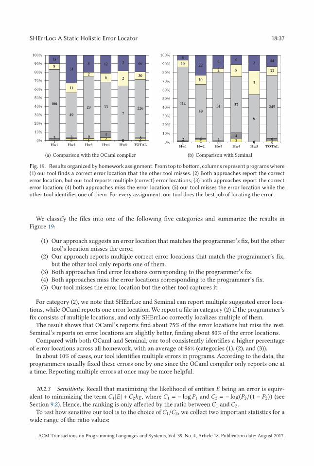
SHErrLoc: A Static Holistic Error Locator 18:37
Fig. 19. Results organized by homework assignment. From top to bottom, columns represent programs where
(1) our tool finds a correct error location that the other tool misses. (2) Both approaches report the correct
error location, but our tool reports multiple (correct) error locations; (3) both approaches report the correct
error location; (4) both approaches miss the error location; (5) our tool misses the error location while the
other tool identifies one of them. For every assignment, our tool does the best job of locating the error.
We classify the files into one of the following five categories and summarize the results inFigure 19:
(1) Our approach suggests an error location that matches the programmer’s fix, but the othertool’s location misses the error.
(2) Our approach reports multiple correct error locations that match the programmer’s fix,but the other tool only reports one of them.
(3) Both approaches find error locations corresponding to the programmer’s fix.(4) Both approaches miss the error locations corresponding to the programmer’s fix.(5) Our tool misses the error location but the other tool captures it.
For category (2), we note that SHErrLoc and Seminal can report multiple suggested error loca-tions, while OCaml reports one error location. We report a file in category (2) if the programmer’sfix consists of multiple locations, and only SHErrLoc correctly localizes multiple of them.
The result shows that OCaml’s reports find about 75% of the error locations but miss the rest.Seminal’s reports on error locations are slightly better, finding about 80% of the error locations.
Compared with both OCaml and Seminal, our tool consistently identifies a higher percentageof error locations across all homework, with an average of 96% (categories (1), (2), and (3)).
In about 10% of cases, our tool identifies multiple errors in programs. According to the data, theprogrammers usually fixed these errors one by one since the OCaml compiler only reports one ata time. Reporting multiple errors at once may be more helpful.
10.2.3 Sensitivity. Recall that maximizing the likelihood of entities E being an error is equiv-alent to minimizing the term C1 |E | +C2kE , where C1 = − log P1 and C2 = − log(P2/(1 − P2)) (seeSection 9.2). Hence, the ranking is only affected by the ratio between C1 and C2.
To test how sensitive our tool is to the choice ofC1/C2, we collect two important statistics for awide range of the ratio values:
ACM Transactions on Programming Languages and Systems, Vol. 39, No. 4, Article 18. Publication date: August 2017.
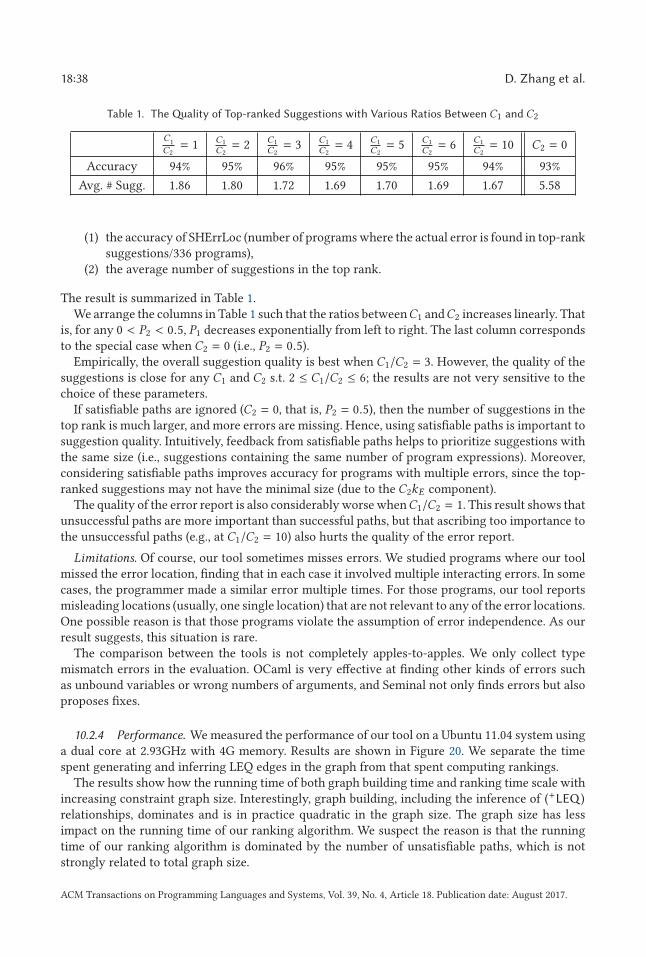
18:38 D. Zhang et al.
Table 1. The Quality of Top-ranked Suggestions with Various Ratios Between C1 and C2
C1
C2= 1 C1
C2= 2 C1
C2= 3 C1
C2= 4 C1
C2= 5 C1
C2= 6 C1
C2= 10 C2 = 0
Accuracy 94% 95% 96% 95% 95% 95% 94% 93%
Avg. # Sugg. 1.86 1.80 1.72 1.69 1.70 1.69 1.67 5.58
(1) the accuracy of SHErrLoc (number of programs where the actual error is found in top-ranksuggestions/336 programs),
(2) the average number of suggestions in the top rank.
The result is summarized in Table 1.We arrange the columns in Table 1 such that the ratios betweenC1 andC2 increases linearly. That
is, for any 0 < P2 < 0.5, P1 decreases exponentially from left to right. The last column correspondsto the special case when C2 = 0 (i.e., P2 = 0.5).
Empirically, the overall suggestion quality is best when C1/C2 = 3. However, the quality of thesuggestions is close for any C1 and C2 s.t. 2 ≤ C1/C2 ≤ 6; the results are not very sensitive to thechoice of these parameters.
If satisfiable paths are ignored (C2 = 0, that is, P2 = 0.5), then the number of suggestions in thetop rank is much larger, and more errors are missing. Hence, using satisfiable paths is important tosuggestion quality. Intuitively, feedback from satisfiable paths helps to prioritize suggestions withthe same size (i.e., suggestions containing the same number of program expressions). Moreover,considering satisfiable paths improves accuracy for programs with multiple errors, since the top-ranked suggestions may not have the minimal size (due to the C2kE component).
The quality of the error report is also considerably worse whenC1/C2 = 1. This result shows thatunsuccessful paths are more important than successful paths, but that ascribing too importance tothe unsuccessful paths (e.g., at C1/C2 = 10) also hurts the quality of the error report.
Limitations. Of course, our tool sometimes misses errors. We studied programs where our toolmissed the error location, finding that in each case it involved multiple interacting errors. In somecases, the programmer made a similar error multiple times. For those programs, our tool reportsmisleading locations (usually, one single location) that are not relevant to any of the error locations.One possible reason is that those programs violate the assumption of error independence. As ourresult suggests, this situation is rare.
The comparison between the tools is not completely apples-to-apples. We only collect typemismatch errors in the evaluation. OCaml is very effective at finding other kinds of errors suchas unbound variables or wrong numbers of arguments, and Seminal not only finds errors but alsoproposes fixes.
10.2.4 Performance. We measured the performance of our tool on a Ubuntu 11.04 system usinga dual core at 2.93GHz with 4G memory. Results are shown in Figure 20. We separate the timespent generating and inferring LEQ edges in the graph from that spent computing rankings.
The results show how the running time of both graph building time and ranking time scale withincreasing constraint graph size. Interestingly, graph building, including the inference of (+LEQ )relationships, dominates and is in practice quadratic in the graph size. The graph size has lessimpact on the running time of our ranking algorithm. We suspect the reason is that the runningtime of our ranking algorithm is dominated by the number of unsatisfiable paths, which is notstrongly related to total graph size.
ACM Transactions on Programming Languages and Systems, Vol. 39, No. 4, Article 18. Publication date: August 2017.
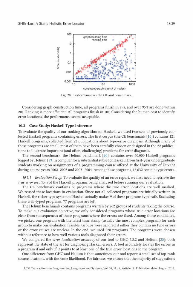
SHErrLoc: A Static Holistic Error Locator 18:39
Fig. 20. Performance on the OCaml benchmark.
Considering graph construction time, all programs finish in 79s, and over 95% are done within20s. Ranking is more efficient: All programs finish in 10s. Considering the human cost to identifyerror locations, the performance seems acceptable.
10.3 Case Study: Haskell Type Inference
To evaluate the quality of our ranking algorithm on Haskell, we used two sets of previously col-lected Haskell programs containing errors. The first corpus (the CE benchmark [10]) contains 121Haskell programs, collected from 22 publications about type-error diagnosis. Although many ofthese programs are small, most of them have been carefully chosen or designed in the 22 publica-tions to illustrate important (and often, challenging) problems for error diagnosis.
The second benchmark, the Helium benchmark [20], contains over 50,000 Haskell programslogged by Helium [23], a compiler for a substantial subset of Haskell, from first-year undergraduatestudents working on assignments of a programming course offered at the University of Utrechtduring course years 2002–2003 and 2003–2004. Among these programs, 16,632 contain type errors.
10.3.1 Evaluation Setup. To evaluate the quality of an error report, we first need to retrieve thetrue error locations of the Haskell programs being analyzed before running our evaluation.
The CE benchmark contains 86 programs where the true error locations are well marked.We reused these locations in evaluation. Since not all collected programs are initially written inHaskell, the richer type system of Haskell actually makes 9 of these programs type-safe. Excludingthese well-typed programs, 77 programs are left.
The Helium benchmark contains programs written by 262 groups of students taking the course.To make our evaluation objective, we only considered programs whose true error locations areclear from subsequences of those programs where the errors are fixed. Among those candidates,we picked one program with the latest time stamp (usually the most complex program) for eachgroup to make our evaluation feasible. Groups were ignored if either they contain no type errorsor the error causes are unclear. In the end, we used 228 programs. The programs were chosenwithout reference to how well various tools diagnosed their errors.
We compared the error localization accuracy of our tool to GHC 7.8.2 and Helium [25]; bothrepresent the state of the art for diagnosing Haskell errors. A tool accurately locates the errors ina program if and only if it points to at least one of the true error locations in the program.
One difference from GHC and Helium is that sometimes, our tool reports a small set of top-ranksource locations, with the same likelihood. For fairness, we ensure that the majority of suggestions
ACM Transactions on Programming Languages and Systems, Vol. 39, No. 4, Article 18. Publication date: August 2017.
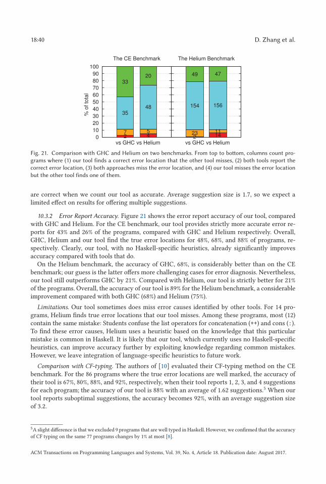
18:40 D. Zhang et al.
Fig. 21. Comparison with GHC and Helium on two benchmarks. From top to bottom, columns count pro-
grams where (1) our tool finds a correct error location that the other tool misses, (2) both tools report the
correct error location, (3) both approaches miss the error location, and (4) our tool misses the error location
but the other tool finds one of them.
are correct when we count our tool as accurate. Average suggestion size is 1.7, so we expect alimited effect on results for offering multiple suggestions.
10.3.2 Error Report Accuracy. Figure 21 shows the error report accuracy of our tool, comparedwith GHC and Helium. For the CE benchmark, our tool provides strictly more accurate error re-ports for 43% and 26% of the programs, compared with GHC and Helium respectively. Overall,GHC, Helium and our tool find the true error locations for 48%, 68%, and 88% of programs, re-spectively. Clearly, our tool, with no Haskell-specific heuristics, already significantly improvesaccuracy compared with tools that do.
On the Helium benchmark, the accuracy of GHC, 68%, is considerably better than on the CEbenchmark; our guess is the latter offers more challenging cases for error diagnosis. Nevertheless,our tool still outperforms GHC by 21%. Compared with Helium, our tool is strictly better for 21%of the programs. Overall, the accuracy of our tool is 89% for the Helium benchmark, a considerableimprovement compared with both GHC (68%) and Helium (75%).
Limitations. Our tool sometimes does miss error causes identified by other tools. For 14 pro-grams, Helium finds true error locations that our tool misses. Among these programs, most (12)contain the same mistake: Students confuse the list operators for concatenation (++) and cons (:).To find these error causes, Helium uses a heuristic based on the knowledge that this particularmistake is common in Haskell. It is likely that our tool, which currently uses no Haskell-specificheuristics, can improve accuracy further by exploiting knowledge regarding common mistakes.However, we leave integration of language-specific heuristics to future work.
Comparison with CF-typing. The authors of [10] evaluated their CF-typing method on the CEbenchmark. For the 86 programs where the true error locations are well marked, the accuracy oftheir tool is 67%, 80%, 88%, and 92%, respectively, when their tool reports 1, 2, 3, and 4 suggestionsfor each program; the accuracy of our tool is 88% with an average of 1.62 suggestions.5 When ourtool reports suboptimal suggestions, the accuracy becomes 92%, with an average suggestion sizeof 3.2.
5A slight difference is that we excluded 9 programs that are well typed in Haskell. However, we confirmed that the accuracy
of CF typing on the same 77 programs changes by 1% at most [8].
ACM Transactions on Programming Languages and Systems, Vol. 39, No. 4, Article 18. Publication date: August 2017.
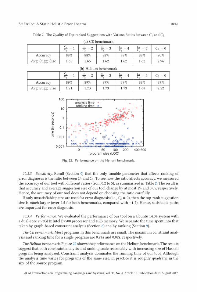
SHErrLoc: A Static Holistic Error Locator 18:41
Table 2. The Quality of Top-ranked Suggestions with Various Ratios between C1 and C2
(a) CE benchmarkC1
C2= 1 C1
C2= 2 C1
C2= 3 C1
C2= 4 C1
C2= 5 C2 = 0
Accuracy 88% 88% 88% 88% 88% 90%
Avg. Sugg. Size 1.62 1.65 1.62 1.62 1.62 2.96
(b) Helium benchmarkC1
C2= 1 C1
C2= 2 C1
C2= 3 C1
C2= 4 C1
C2= 5 C2 = 0
Accuracy 89% 89% 89% 89% 88% 87%
Avg. Sugg. Size 1.71 1.73 1.73 1.73 1.68 2.52
Fig. 22. Performance on the Helium benchmark.
10.3.3 Sensitivity. Recall (Section 9) that the only tunable parameter that affects ranking oferror diagnoses is the ratio betweenC2 andC1. To see how the ratio affects accuracy, we measuredthe accuracy of our tool with different ratios (from 0.2 to 5), as summarized in Table 2. The result isthat accuracy and average suggestion size of our tool change by at most 1% and 0.05, respectively.Hence, the accuracy of our tool does not depend on choosing the ratio carefully.
If only unsatisfiable paths are used for error diagnosis (i.e.,C2 = 0), then the top-rank suggestionsize is much larger (over 2.5 for both benchmarks, compared with ∼1.7). Hence, satisfiable pathsare important for error diagnosis.
10.3.4 Performance. We evaluated the performance of our tool on a Ubuntu 14.04 system witha dual-core 2.93GHz Intel E7500 processor and 4GB memory. We separate the time spent into thattaken by graph-based constraint analysis (Section 6) and by ranking (Section 9).
The CE benchmark. Most programs in this benchmark are small. The maximum constraint anal-ysis and ranking time for a single program are 0.24s and 0.02s, respectively.
The Helium benchmark. Figure 22 shows the performance on the Helium benchmark. The resultssuggest that both constraint analysis and ranking scale reasonably with increasing size of Haskellprogram being analyzed. Constraint analysis dominates the running time of our tool. Althoughthe analysis time varies for programs of the same size, in practice it is roughly quadratic in thesize of the source program.
ACM Transactions on Programming Languages and Systems, Vol. 39, No. 4, Article 18. Publication date: August 2017.
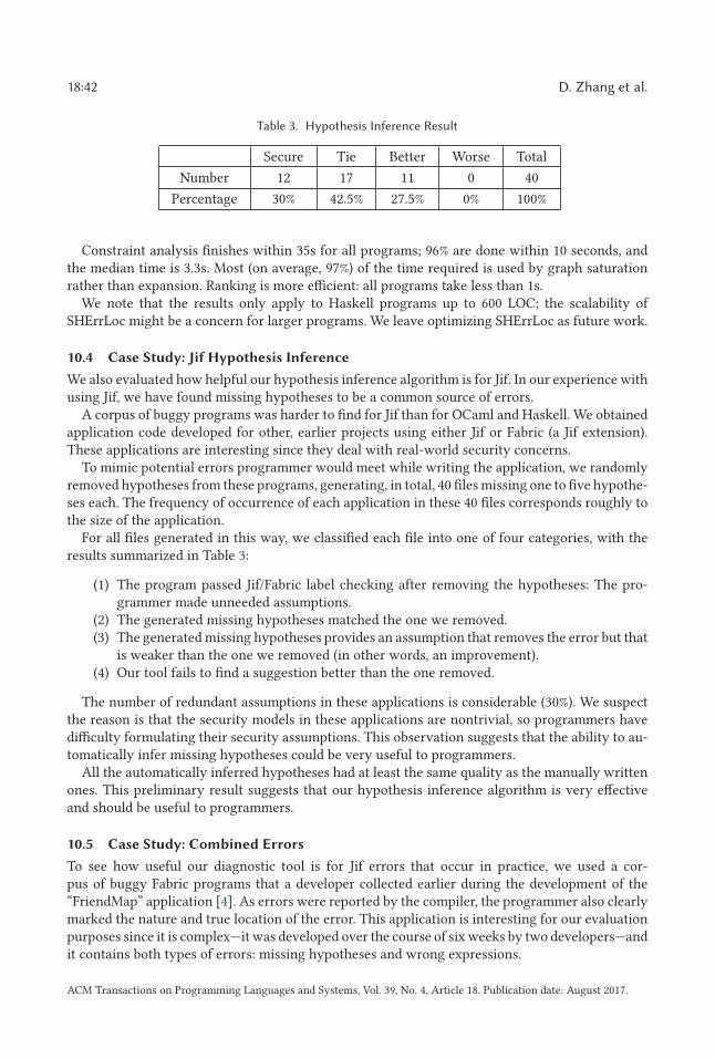
18:42 D. Zhang et al.
Table 3. Hypothesis Inference Result
Secure Tie Better Worse Total
Number 12 17 11 0 40
Percentage 30% 42.5% 27.5% 0% 100%
Constraint analysis finishes within 35s for all programs; 96% are done within 10 seconds, andthe median time is 3.3s. Most (on average, 97%) of the time required is used by graph saturationrather than expansion. Ranking is more efficient: all programs take less than 1s.
We note that the results only apply to Haskell programs up to 600 LOC; the scalability ofSHErrLoc might be a concern for larger programs. We leave optimizing SHErrLoc as future work.
10.4 Case Study: Jif Hypothesis Inference
We also evaluated how helpful our hypothesis inference algorithm is for Jif. In our experience withusing Jif, we have found missing hypotheses to be a common source of errors.
A corpus of buggy programs was harder to find for Jif than for OCaml and Haskell. We obtainedapplication code developed for other, earlier projects using either Jif or Fabric (a Jif extension).These applications are interesting since they deal with real-world security concerns.
To mimic potential errors programmer would meet while writing the application, we randomlyremoved hypotheses from these programs, generating, in total, 40 files missing one to five hypothe-ses each. The frequency of occurrence of each application in these 40 files corresponds roughly tothe size of the application.
For all files generated in this way, we classified each file into one of four categories, with theresults summarized in Table 3:
(1) The program passed Jif/Fabric label checking after removing the hypotheses: The pro-grammer made unneeded assumptions.
(2) The generated missing hypotheses matched the one we removed.(3) The generated missing hypotheses provides an assumption that removes the error but that
is weaker than the one we removed (in other words, an improvement).(4) Our tool fails to find a suggestion better than the one removed.
The number of redundant assumptions in these applications is considerable (30%). We suspectthe reason is that the security models in these applications are nontrivial, so programmers havedifficulty formulating their security assumptions. This observation suggests that the ability to au-tomatically infer missing hypotheses could be very useful to programmers.
All the automatically inferred hypotheses had at least the same quality as the manually writtenones. This preliminary result suggests that our hypothesis inference algorithm is very effectiveand should be useful to programmers.
10.5 Case Study: Combined Errors
To see how useful our diagnostic tool is for Jif errors that occur in practice, we used a cor-pus of buggy Fabric programs that a developer collected earlier during the development of the“FriendMap” application [4]. As errors were reported by the compiler, the programmer also clearlymarked the nature and true location of the error. This application is interesting for our evaluationpurposes since it is complex—it was developed over the course of six weeks by two developers—andit contains both types of errors: missing hypotheses and wrong expressions.
ACM Transactions on Programming Languages and Systems, Vol. 39, No. 4, Article 18. Publication date: August 2017.
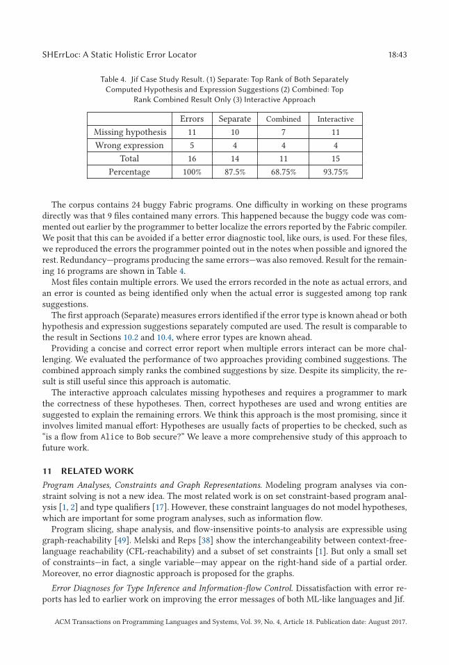
SHErrLoc: A Static Holistic Error Locator 18:43
Table 4. Jif Case Study Result. (1) Separate: Top Rank of Both Separately
Computed Hypothesis and Expression Suggestions (2) Combined: Top
Rank Combined Result Only (3) Interactive Approach
Errors Separate Combined Interactive
Missing hypothesis 11 10 7 11
Wrong expression 5 4 4 4
Total 16 14 11 15
Percentage 100% 87.5% 68.75% 93.75%
The corpus contains 24 buggy Fabric programs. One difficulty in working on these programsdirectly was that 9 files contained many errors. This happened because the buggy code was com-mented out earlier by the programmer to better localize the errors reported by the Fabric compiler.We posit that this can be avoided if a better error diagnostic tool, like ours, is used. For these files,we reproduced the errors the programmer pointed out in the notes when possible and ignored therest. Redundancy—programs producing the same errors—was also removed. Result for the remain-ing 16 programs are shown in Table 4.
Most files contain multiple errors. We used the errors recorded in the note as actual errors, andan error is counted as being identified only when the actual error is suggested among top ranksuggestions.
The first approach (Separate) measures errors identified if the error type is known ahead or bothhypothesis and expression suggestions separately computed are used. The result is comparable tothe result in Sections 10.2 and 10.4, where error types are known ahead.
Providing a concise and correct error report when multiple errors interact can be more chal-lenging. We evaluated the performance of two approaches providing combined suggestions. Thecombined approach simply ranks the combined suggestions by size. Despite its simplicity, the re-sult is still useful since this approach is automatic.
The interactive approach calculates missing hypotheses and requires a programmer to markthe correctness of these hypotheses. Then, correct hypotheses are used and wrong entities aresuggested to explain the remaining errors. We think this approach is the most promising, since itinvolves limited manual effort: Hypotheses are usually facts of properties to be checked, such as“is a flow from Alice to Bob secure?” We leave a more comprehensive study of this approach tofuture work.
11 RELATED WORK
Program Analyses, Constraints and Graph Representations. Modeling program analyses via con-straint solving is not a new idea. The most related work is on set constraint-based program anal-ysis [1, 2] and type qualifiers [17]. However, these constraint languages do not model hypotheses,which are important for some program analyses, such as information flow.
Program slicing, shape analysis, and flow-insensitive points-to analysis are expressible usinggraph-reachability [49]. Melski and Reps [38] show the interchangeability between context-free-language reachability (CFL-reachability) and a subset of set constraints [1]. But only a small setof constraints—in fact, a single variable—may appear on the right-hand side of a partial order.Moreover, no error diagnostic approach is proposed for the graphs.
Error Diagnoses for Type Inference and Information-flow Control. Dissatisfaction with error re-ports has led to earlier work on improving the error messages of both ML-like languages and Jif.
ACM Transactions on Programming Languages and Systems, Vol. 39, No. 4, Article 18. Publication date: August 2017.
18:44 D. Zhang et al.
Efforts on improving type-error messages in ML-like languages can be traced to the early workof Wand [55] and of Johnson and Walz [27]. These two pieces of work represent two directions inimproving error messages: The former traces everything that contributes to the error, whereas thelatter attempts to infer the most likely cause. We only discuss the most related among them, butHeeren’s summary [24] provides more details.
In the first direction, several efforts [11, 17, 19, 48, 52] improve the basic idea of Wand [55]in various ways. Despite the attractiveness of feeding a full explanation to the programmer, thereports are usually verbose and hard to follow [24].
In the second direction, one approach is to alter the order of type unification [9, 30, 36]. But sincethe error location may be used anywhere during the unification procedure, any specific order failsin some circumstance. Some prior work [21, 24, 27, 34, 45] also builds on constraints, but theseconstraint languages at most have limited support for sophisticated features such as type classes,type signatures, type families, and GADTs. Most of these approaches also use language-specificheuristics to improve report quality. For example, the accuracy of MinErrLoc [45] depends on theapplication-specific weight assigned to each constraint, while the accuracy of Mycroft [34] dependson the identification of certain hard constraints (i.e., constraints that should never be blamed) forOCaml type inference. As reported by Loncaric et al. [34], SHErrLoc achieves at least comparableaccuracy on OCaml programs while treating all constraints as equally likely to be wrong.
A third approach is to generate fixes for errors by searching for similar programs [31, 37] ortype substitutions [10] that do type-check. Unfortunately, we cannot obtain a common corpus toperform direct comparison with McAdam [37]. We are able to compare directly with the workof [31]; the results of Section 10.2 suggest that SHErrLoc improves on accuracy of [31] by 10%.Moreover, the results on the CE benchmark (Section 10.3.2) suggest that our tool localizes true errorlocations more accurately than the prior approach of Chen and Erwig [10]. Although SHErrLoccurrently does not provide suggested fixes, accurate error localization is likely to provide goodplaces to search for fixes. Combining these two techniques may be a fruitful area for future work.
For information-flow control, King et al. [28] propose to generate a trace explaining theinformation-flow violation. Although this approach also constructs a diagnosis from a dependencygraph, only a subset of the DLM model is handled. As in type-error slicing, reporting whole pathscan yield very verbose error reports. Recent work by Weijers et al. [57] diagnoses information-flow violations in a higher-order, polymorphic language. But the mechanism is based on tailoredheuristics and a more limited constraint language. Moreover, the algorithm in [57] diagnoses asingle unsatisfiable path, while our algorithm diagnoses multiple errors.
Probabilistic Inference. Applying probabilistic inference to program analysis has appeared in ear-lier work, particularly on specification inference [29, 33]. Our contribution is to apply probabilisticinference to a general class of static analyses, allowing errors to be localized without language-specific tuning. Also related is work on statistical methods for diagnosing dynamic errors (e.g., [32,60]). These algorithms rely on a different principle—statistical interpretation—and do not handleimportant features for static analysis, such as constructors and hypotheses.
The work of Ball et al. [5] on diagnosing errors detected by model checking has exploited a sim-ilar insight by using information about traces for both correct execution and for errors to localizeerror causes. Beyond differences in context, that work differs in not actually using probabilisticinference; each error trace is considered in isolation, and transitions are not flagged as causes ifthey lie on any correct trace.
Missing Hypothesis Inference. The most related work on inferring likely missing hypotheses isthe recent work by Dillig et al. [14] on error diagnosis using abductive inference. This work com-putes small, relevant queries presented to a user that capture exactly the information a program
ACM Transactions on Programming Languages and Systems, Vol. 39, No. 4, Article 18. Publication date: August 2017.

SHErrLoc: A Static Holistic Error Locator 18:45
analysis is missing to either discharge or validate the error. It does not attempt to identify incorrectconstraints.
With regard to hypothesis inference, the Dillig algorithm infers missing hypotheses for a singleassertion, whereas our tool finds missing hypotheses that satisfy a set of assertions. Further, theDillig algorithm infers additional invariants on variables (e.g., x ≤ 3 for a constraint variable x ),while our algorithm also infers missing partial orderings on constructors (such as Alice ≤ Bob inSection 9.3.1).
Recent work by Blackshear and Lahiri [7] assigns confidence to errors reported by modular as-sertion checkers. This is done by the computation of an almost-correct specification that is usedto identify errors likely to be false positives. This idea is largely complementary to our approach:although their algorithm returns a set of high-confidence errors, it does not attempt to infer theirlikely cause. At least for some program analyses, the heuristics they develop might also be use-ful for classifying whether errors result from missing hypotheses or from wrong constraints. Aswith the comparison to Dillig et al. [14], our algorithm also infers missing partial orderings onconstructors, not just additional specifications on variables.
12 CONCLUSION
Better tools for helping programmers locate the errors detected by type systems and other programanalyses should help adoption of the many powerful program analyses that have been developed.The science of diagnosing programmer errors is still in its infancy, but this article takes a steptowards improving the situation. Our analysis of program constraint graphs offers a general, prin-cipled way to identify both incorrect expressions and missing assumptions. Results on three verydifferent languages, OCaml, Haskell, and Jif, with no language-specific customization, suggest thisapproach is promising and broadly applicable.
There are many interesting directions to take this work. Though we have shown that the tech-nique works well on three very different type systems, it would likely be fruitful to apply theseideas to other type systems and program analyses, such as dataflow analysis and points-to analysis,as we sketched in this article, and to explore more sophisticated ways to estimate the likelihoodof different error explanations by incorporating prior knowledge about likely errors.
REFERENCES
[1] Alexander Aiken. 1999. Introduction to set constraint-based program analysis. Sci. Comput. Program. 35, 2–3 (1999),
79–111.
[2] Alexander Aiken and Edward L. Wimmers. 1993. Type inclusion constraints and type inference. In Proceedings of the
Conference on Functional Programming Languages and Computer Architecture. 31–41.
[3] Lars Ole Andersen. 1994. Program Analysis and Specialization for the C Programming Language. Ph.D. Dissertation.
DIKU, University of Copenhagen.
[4] Owen Arden, Michael D. George, Jed Liu, K. Vikram, Aslan Askarov, and Andrew C. Myers. 2012. Sharing mobile
code securely with information flow control. In Proceedings of the IEEE Symposium on Security and Privacy. 191–205.
[5] Thomas Ball, Mayur Naik, and Sriram Rajamani. 2003. From symptom to cause: Localizing errors in counterexample
traces. In Proceedings of the ACM Symposium on Principles of Programming Languages (POPL’03). 97–105.
[6] Chris Barrett, Riko Jacob, and Madhav Marathe. 2000. Formal-language-constrained path problems. SIAM J. Comput.
30, 3 (2000), 809–837.
[7] Sam Blackshear and Shuvendu K. Lahiri. 2013. Almost-correct specifications: A modular semantic framework for
assigning confidence to warnings. In Proceedings of the ACM SIGPLAN Conference on Programming Language Design
and Implementation (PLDI’13). 209–218.
[8] Shen Chen. 2014. Accuracy of CF-Typing. Private communication. (2014).
[9] Sheng Chen and Martin Erwig. 2014. Better Type-Error Messages Through Lazy Typing. Technical Report. Oregon State
University.
[10] Sheng Chen and Martin Erwig. 2014. Counter-factual typing for debugging type errors. In Proceedings of the ACM
Symposium on Principles of Programming Languages (POPL’14).
ACM Transactions on Programming Languages and Systems, Vol. 39, No. 4, Article 18. Publication date: August 2017.
18:46 D. Zhang et al.
[11] Venkatesh Choppella and Christopher T. Haynes. 1995. Diagnosis of Ill-typed Programs. Technical Report. Indiana
University.
[12] Luis Manuel Martins Damas. 1985. Type Assignment in Programming Languages. Ph.D. Dissertation. Department of
Computer Science, University of Edinburgh.
[13] Dorothy E. Denning. 1976. A Lattice model of secure information flow. Commun. ACM 19, 5 (1976), 236–243.
[14] Isil Dillig, Thomas Dillig, and Alex Aiken. 2012. Automated error diagnosis using abductive inference. In Proceedings
of the ACM SIGPLAN Conference on Programming Language Design and Implementation (PLDI’12). 181–192.
[15] EasyOCaml. 2009. EasyOCaml. Retrieved from http://easyocaml.forge.ocamlcore.org.
[16] Jeffrey S. Foster, Manuel Fahndrich, and Alexander Aiken. 1997. Flow-Insensitive Points-to Analysis with Term and Set
Constraints. Technical Report. Berkeley, CA, USA.
[17] Jeffrey S. Foster, Robert Johnson, John Kodumal, and Alex Aiken. 2006. Flow-insensitive type qualifiers. ACM Trans.
Program. Lang. Syst. 28, 6 (Nov. 2006), 1035–1087.
[18] Andrew Gelman, John B. Carlin, Hal S. Stern, and Donald B. Rubin. 2004. Bayesian Data Analysis (2nd ed.). Chapman
& Hall/CRC.
[19] Christian Haack and J. B. Wells. 2004. Type error slicing in implicitly typed higher-order languages. Sci. Comput.
Program. 50, 1–3 (2004), 189–224.
[20] Jurriaan Hage. 2014. Helium benchmark programs (2002–2005). Private communication. (2014).
[21] Jurriaan Hage and Bastiaan Heeren. 2007. Heuristics for type error discovery and recovery. In Implementation and
Application of Functional Languages, Zoltán Horváth, Viktória Zsók, and Andrew Butterfield (Eds.). Lecture Notes in
Computer Science, Vol. 4449. Springer, 199–216.
[22] P. E. Hart, N. J. Nilsson, and B. Raphael. 1968. A formal basis for the heuristic determination of minimum cost paths.
IEEE Trans Syst. Sci. Cybernet. 4, 2 (1968), 100–107.
[23] Bastiaan Heeren, Daan Leijen, and Arjan van IJzendoorn. 2003. Helium, for learning Haskell. In Proceedings of the
2003 ACM SIGPLAN Workshop on Haskell. 62–71.
[24] Bastiaan J. Heeren. 2005. Top Quality Type Error Messages. Ph.D. Dissertation. Universiteit Utrecht, The Netherlands.
[25] Helium 1.8(2014) 2014. Helium (ver. 1.8). Retrieved from https://hackage.haskell.org/package/helium.
[26] Paul Hudak, Simon Peyton Jones, and Philip Wadler. 1992. Report on the programming language Haskell. SIGPLAN
Not. 27, 5 (May 1992).
[27] Gregory F. Johnson and Janet A. Walz. 1986. A maximum flow approach to anomaly isolation in unification-based
incremental type inference. In Proceedings of the ACM Symposium on Principles of Programming Languages (POPL’86).
44–57.
[28] Dave King, Trent Jaeger, Somesh Jha, and Sanjit A. Seshia. 2008. Effective blame for information-flow violations. In
Proceedings of the International Symposium on Foundations of Software Engineering. 250–260.
[29] Ted Kremenek, Paul Twohey, Godmar Back, Andrew Ng, and Dawson Engler. 2006. From uncertainty to belief: Infer-
ring the specification within. In Proceedings of the USENIX Symposium on Operating Systems Design and Implementa-
tion (OSDI’06). 161–176. http://dl.acm.org/citation.cfm?id=1298455.1298471
[30] Oukseh Lee and Kwangkeun Yi. 1998. Proofs about a folklore let-polymorphic type inference algorithm. ACM Trans.
Program. Lang. Syst. 20, 4 (July 1998), 707–723. http://doi.acm.org/10.1145/291891.291892
[31] Benjamin S. Lerner, Matthew Flower, Dan Grossman, and Craig Chambers. 2007. Searching for type-error messages.
In Proceedings of the ACM SIGPLAN Conference on Programming Language Design and Implementation (PLDI’07). 425–
434.
[32] Ben Liblit, Mayur Naik, Alice X. Zheng, Alex Aiken, and Michael I. Jordan. 2005. Scalable statistical bug isolation. In
Proceedings of the ACM SIGPLAN Conference on Programming Language Design and Implementation (PLDI’05). 15–26.
[33] Benjamin Livshits, Aditya V. Nori, Sriram K. Rajamani, and Anindya Banerjee. 2009. Merlin: Specification inference
for explicit information flow problems. In Proceedings of the ACM SIGPLAN Conference on Programming Language
Design and Implementation (PLDI’09). 75–86.
[34] Calvin Loncaric, Satish Chandra, Cole Schlesinger, and Manu Sridharan. 2016. A practical framework for type infer-
ence error explanation. 781–799.
[35] Simon Marlow and Simon Peyton-Jones. 1993. The Glasgow Haskell Compiler. Retrieved from http://www.aosabook.
org/en/ghc.html.
[36] Bruce James McAdam. 1998. On the unification of substitutions in type inference. In Implementation of Functional
Languages. 139–154.
[37] Bruce James McAdam. 2001. Repairing Type Errors in Functional Programs. Ph.D. Dissertation. Laboratory for Foun-
dations of Computer Science, The University of Edinburgh.
[38] David Melski and Thomas Reps. 2000. Interconvertibility of a class of set constraints and context-free language reach-
ability. Theoret. Comput. Sci. 248, 1–2 (2000), 29–98.
ACM Transactions on Programming Languages and Systems, Vol. 39, No. 4, Article 18. Publication date: August 2017.
SHErrLoc: A Static Holistic Error Locator 18:47
[39] Robin Milner, Mads Tofte, and Robert Harper. 1990. The Definition of Standard ML. MIT Press, Cambridge, MA.
[40] Andrew C. Myers and Barbara Liskov. 1997. A decentralized model for information flow control. In Proceedings of the
ACM Symposium on Operating System Principles (SOSP’97). 129–142.
[41] Andrew C. Myers, Lantian Zheng, Steve Zdancewic, Stephen Chong, and Nathaniel Nystrom. 2006. Jif 3.0: Java In-
formation Flow. Software release, www.cs.cornell.edu/jif. (July 2006).
[42] Anil Nerode and Richard Shore. 1997. Logic for Applications (2nd ed.). Springer, New York, NY.
[43] OCaml. 2016. OCaml programming language. Retrieved from http://ocaml.org.
[44] Martin Odersky, Martin Sulzmann, and Martin Wehr. 1999. Type inference with constrained types. Theor. Pract. Object
Syst. 5, 1 (Jan. 1999), 35–55. http://dx.doi.org/10.1002/(SICI)1096-9942(199901/03)5:1〈35::AID-TAPO4〉3.0.CO; 2-4
[45] Zvonimir Pavlinovic, Tim King, and Thomas Wies. 2014. Finding minimum type error sources. In Proceedings of the
2014 ACM SIGPLAN Conference on Object-Oriented Programming, Systems, Languages and Applications (OOPSLA’14).
525–542.
[46] Simon Peyton Jones, Dimitrios Vytiniotis, Stephanie Weirich, and Mark Shields. 2007. Practical type inference for
arbitrary-rank types. J. Funct. Program. 17, 1 (Jan. 2007), 1–82. DOI:https://doi.org/10.1017/S0956796806006034
[47] Francois Pottier and Didier Rémy. 2005. The essence of ML type inference. In Advanced Topics in Types and Program-
ming Languages, Benjamin C. Pierce (Ed.). MIT Press, 389–489.
[48] Vincent Rahli, J. B. Wells, and Fairouz Kamareddine. 2010. A Constraint System for a SML Type Error Slicer. Technical
Report HW-MACS-TR-0079. Heriot-Watt University.
[49] Thomas Reps. 1998. Program analysis via graph reachability. Info. Softw. Technol. 40, 11–12 (1998), 701–726.
[50] SHErrLoc. 2014. SHErrLoc (Static Holistic Error Locator) Tool Release (ver 1.0). Retrieved from http://www.cs.cornell.
edu/projects/sherrloc.
[51] Bjarne Steensgaard. 1996. Points-to analysis in almost linear time. In Proceedings of the ACM Symposium on Principles
of Programming Languages (POPL’96). 32–41. http://doi.acm.org/10.1145/237721.237727
[52] Frank Tip and T. B. Dinesh. 2001. A slicing-based approach for locating type errors. ACM Trans. Softw. Eng. Methodol.
10, 1 (2001), 5–55.
[53] Dimitrios Vytiniotis, Simon Peyton Jones, Tom Schrijvers, and Martin Sulzmann. 2011. OutsideIn(X): Modular type
inference with local assumptions. J. Funct. Program. 21, 4–5 (2011), 333–412.
[54] Dimitrios Vytiniotis, Simon Peyton Jones, and Tom Schrijvers. 2010. Let should not be generalized. In Proceedings
of the 5th ACM SIGPLAN Workshop on Types in Language Design and Implementation. ACM, New York, NY, 39–50.
DOI:https://doi.org/10.1145/1708016.1708023
[55] Mitchell Wand. 1986. Finding the source of type errors. In Proceedings of the ACM Symposium on Principles of Pro-
gramming Languages (POPL’86).
[56] Mitchell Wand. 1987. A simple algorithm and proof for type inference. Fundam. Inform. 10, 2 (1987), 115–122.
[57] Jeroen Weijers, Jurriaan Hage, and Stefan Holdermans. 2013. Security type error diagnosis for higher-order, poly-
morphic languages. In Proceedings of the ACM SIGPLAN Workshop on Partial Evaluation and Program Manipulation.
3–12. http://doi.acm.org/10.1145/2426890.2426894
[58] Danfeng Zhang and Andrew C. Myers. 2014. Toward general diagnosis of static errors. In Proceedings of the ACM
Symposium on Principles of Programming Languages (POPL’14). 569–581. http://www.cs.cornell.edu/andru/papers/
diagnostic.
[59] Danfeng Zhang, Andrew C. Myers, Dimitrios Vytiniotis, and Simon Peyton Jones. 2015. Diagnosing type errors with
class. In Proceedings of the ACM SIGPLAN Conference on Programming Language Design and Implementation (PLDI’15).
12–21.
[60] Alice X. Zheng, Ben Liblit, and Mayur Naik. 2006. Statistical debugging: Simultaneous identification of multiple bugs.
In Proceedings of the International Conference on Machine Learning (ICML’06). 1105–1112.
Received August 2016; revised June 2017; accepted June 2017
ACM Transactions on Programming Languages and Systems, Vol. 39, No. 4, Article 18. Publication date: August 2017.


![[ACM-ICPC] 0 - ACM-ICPC](https://static.fdocuments.net/doc/165x107/555603ead8b42a3f168b4838/acm-icpc-0-acm-icpc.jpg)