
RENATO LEONI - UniFIlocal.disia.unifi.it/leoni/analisi_dati/metodi/cca.pdf · RENATO LEONI...
40
RENATO LEONI Canonical Correlation Analysis UNIVERSITY OF FLORENCE DEPARTMENT OF STATISTICS "G. PARENTI" FLORENCE, 2007
Transcript of RENATO LEONI - UniFIlocal.disia.unifi.it/leoni/analisi_dati/metodi/cca.pdf · RENATO LEONI...

RENATO LEONI
Canonical Correlation Analysis
UNIVERSITY OF FLORENCE
DEPARTMENT OF STATISTICS "G. PARENTI"
FLORENCE, 2007

This paper is intended for a personal use only. Trading is not
allowed.

CANONICAL CORRELATION ANALYSIS 3
1 INTRODUCTION
In analysing a data matrix such as that considered in PCA, it is often
possible to recognize homogeneous sets of variables (e.g., economic, de-
mographic, social), each set representing a certain aspect of the phenom-
enon under study.
The focus of canonical correlation analysis (CCA) is on the study of
relationships among these sets of variables by an appropriate synthesis of
the original variables of each set, providing at the same time the researcher
with a graphical representation of results on a subspace of low dimension
(usually one or two).
It may be worth adding that, although the applications of CCA are rather
limited since the interpretation of results is often difficult, CCA provides a
general framework for many multidimensional methods like regression,
discriminant analysis and correspondence analysis, which are all special
cases of CCA.
Unlike other approaches to CCA, in this paper no reference to an under-
lying probabilistic model will be done. Moreover, we will confine ourselves
to considering the case of two sets of variables.
The contents of the paper can be summarized as follows.
In Section 2, the basic data and their algebraic structure are introduced.
In Section 3, an approach to CCA is presented. In Section 4, rules for a
graphical representation of results are given. Finally, in Section 5, other
approaches to CCA are set out (1).
(1) Numerical examples, based both on fictitiuos and real data, are provided apart. Relevant alge-braic concepts are stated in [17].
4 RENATO LEONI
2 BASIC DATA AND THEIR ALGEBRAIC STRUCTURE
2.1 BASIC DATA
Consider the matrix
X = x1 1 x1 p
xn1 xnp
where xi j (i = 1, ... , n; j = 1, ... , p) denotes the value of the jth quantitative
variable observed on the ith individual (2).
Setting (j = 1, ... , p)
x j = x1 j
xn j
and (i = 1, ... , n)
x i = x i 1
x ip
,
we can write
X = x1 xp
and
X' = x1 xn .
Considering the notation just introduced, we say that x1 , ... , xp and
x1 , ... , xn represent, respectively, the p variables and the n individuals.
Moreover, suppose that the p variables x1 , ... , xp are partitioned into two
sets − the first consisting of the p1 variables x1 , ... , xp1, the second of the
p2 ≥ p1 variables xp1+ 1 , ... , xp1+ p2 (p1+ p2 = p).
(2) In what follows we consider acquired the main concepts and definitions introduced in [18], partlysummarized here.

CANONICAL CORRELATION ANALYSIS 5
Then, we can write
X = x1 xp1 xp1+ 1 xp1+ p2
= X1 X2 .
2.2 ALGEBRAIC STRUCTURE
With reference to the variables, regarding them as elements of Rn, Rn
(variable space) is equipped with a Euclidean metric in the following way.
As in PCA, the matrix (symmetric and positive definite (p.d.)) of the
Euclidean metric in Rn − with respect to the basis consisting of the n
canonical vectors u 1 , ... , u n − is
M = diag (m1 , ... , m n )
where m i > 0 (i = 1, ... , n), Σ i m i = 1, represents the weight given to the ith
individual and denotes its «importance» in the set of the n individuals.
Since the matrix Y of the p variables measured in terms of deviations
from the means − partitioned in the same way as X − becomes
Y = y1 yp1 yp1+ 1 yp1+ p2 = Y1 Y2 ,
the covariance matrix V of the p variables can be written as
V = Y'MY = Y1' MY1 Y 1' MY2
Y2' MY1 Y 2' MY2
= V1 1 V1 2
V2 1 V2 2
.
Notice that − assuming that r (Y1) = p1 and r (Y2) = p2 − is
r (V1 1) = p1 , r (V2 2) = p2 .
Moreover,
r (V1 2) = r (Y1' MY2) = r (Y1' M1
2M1
2Y2) ≤ min {r (Y1) , r (Y2)} = p1 .
Of course, r (V1 2) = r (V2 1).
We will suppose that r (V1 2) = k > 0. The reasons of this assumption will

6 RENATO LEONI
become apparent from what follows.
With reference to the individuals, regarding them as elements of Rp, Rp
(individual space) is equipped with a Euclidean metric in the following way.
The matrix of the Euclidean metric in Rp − with respect to the basis
consisting of the p canonical vectors u1 , ... , up − is (block Mahalanobis
metric)
Q = diag (V 1 1-1 , V2 2
-1 ) .
Clearly, as V1 1-1 and V2 2
-1 are symmetric and p.d., Q is symmetric and p.d.
too.
The choice of this metric is a natural extension of the choice made in
PCA, where the scope of obtaining homogeneus variances was reached
setting Q = Q1 / σ 2 . Obviously, in the present case, instead of the inverses of
the variances of the variables, it is necessary to consider the inverses of the
covariance matrices of the two sets of variables.
As will be afterwards shown, this choice is coherent with other ways of
presenting CCA (Section 5.2).

CANONICAL CORRELATION ANALYSIS 7
3 AN APPROACH TO CCA
3.1 CANONICAL FACTORS, CANONICAL VARIABLES, AND CANONICAL
CORRELATION COEFFICIENTS
3.1.1 THE FIRST STEP
The first step of the approach to CCA we are considering consists in
determining a linear combination z (1) 1 of y1 , ... , yp1 and a linear combination
z (2) 1 of yp1+ 1 , ... , yp1+ p2 such that the cosine of the angle they form (the linear
correlation coefficient) cos(z (1) 1 , z (2) 1) is a maximum (3).
Setting
z (1) 1 = y 1 a (1) 1 + ... + y p1a (1) p1
= y1 yp1 a (1) 1
a (1) p1
= Y1 a (1) 1 ,
z (2) 1 = y p1+ 1 a (2) p1+ 1 + ... + y p1+ p2a (2) p1+ p2
= yp1+ 1 yp1+ p2 a (2) p1+ 1
a (2) p1+ p2
= Y2 a (2) 1 ,
cos(z (1) 1 , z (2) 1) = cos(Y1a (1) 1 , Y2 a (2) 1)
= a (1) 1' Y1' MY2 a (2) 1
{(a (1) 1' Y1' MY1 a (1) 1)(a (2) 1' Y2' MY2 a (2) 1)}1
2=
a (1) 1' V1 2 a (2) 1
{(a (1) 1' V1 1 a (1) 1)(a (2) 1' V2 2 a (2) 1)}1
2 ,
we have to find out
(1) Max a (1) 1 , a (2) 1
a (1) 1' V1 2 a (2) 1
{(a (1) 1' V1 1 a (1) 1)(a (2) 1' V2 2 a (2) 1)}1
2 .
In order to facilitate the solution of this problem, first it is useful to notice
that cos(z (1) 1 , z (2) 1) is invariant when z (1) 1 (or a (1) 1) is multiplied by c1 and
z (2) 1 (or a (2) 1) is multiplied by c2 , where c1 , c2 are different from zero and of
the same sign.
(3) Coherently with the aim of CCA, principally directed to the study of relationships among setsof variables, we will mainly refer to the solution in the variable space.

8 RENATO LEONI
Therefore, we may consider z (1) 1 and z (2) 1 as vectors of unitary square
length (variance), so (1) is simplified in the following way
(1') Max a (1) 1 , a (2) 1
a (1) 1' V1 2 a (2) 1 , a (1) 1' V1 1 a (1) 1 = 1 , a (2) 1' V2 2 a (2) 1 = 1 .
To solve the problem of constrained maximization set in (1'), consider the
Lagrange function
L(a (1) 1 , a (2) 1 , µ 1 , µ 2) = a (1) 1' V1 2 a (2) 1 − 12
µ 1 (a (1) 1' V1 1 a (1) 1 − 1)
− 12
µ 2 (a (2) 1' V2 2 a (2) 1 − 1)
where µ 1 , µ 2 are Lagrange multipliers.
At (a (1) 1 , a (2) 1 , µ 1 , µ 2) where L(a (1) 1 , a (2) 1 , µ 1 , µ 2) has a maximum, it
must be (4)
∂L∂a (1) 1
(a (1) 1 , a (2) 1 , µ 1 , µ 2)
= V1 2 a (2) 1 − µ 1 V1 1 a (1) 1 = 0
∂L∂a (2) 1
(a (1) 1 , a (2) 1 , µ 1 , µ 2)
= V2 1 a (1) 1 − µ 2 V2 2 a (2) 1 = 0
∂L∂µ 1
(a (1) 1 , a (2) 1 , µ 1 , µ 2)
= a (1) 1' V1 1 a (1) 1 = 1
∂L∂µ 2
(a (1) 1 , a (2) 1 , µ 1 , µ 2)
= a (2) 1' V2 2 a (2) 1 = 1
from which we immediately deduce that
a (1) 1' V1 2 a (2) 1 = µ 1 , a (2) 1' V2 1 a (1) 1 = µ 2
and hence that
a (1) 1' V1 2 a (2) 1 = µ 1 = cos(z (1) 1 , z (2) 1) = µ 2 = a (2) 1' V2 1 a (1) 1 .
Therefore − since it must be
(4) Here and in what follows 0 denotes a zero column vector of appropriate order.
CANONICAL CORRELATION ANALYSIS 9
V1 2 a (2) 1 = cos(z (1) 1 , z (2) 1) V1 1 a (1) 1 , V2 1 a (1) 1 = cos(z (1) 1 , z (2) 1) V2 2 a (2) 1
a (1) 1' V1 1 a (1) 1 = 1 , a (2) 1' V2 2 a (2) 1 = 1
− we realize that cos(z (1) 1 , z (2) 1) and a (1) 1 , a (2) 1 must be found among the
solutions of the system
(2)−r V1 1 V1 2
V2 1 −r V2 2
a (1) 1
a (2) 1 = 0 , a (1) 1' V1 1 a (1) 1 = 1 , a (2) 1' V2 2 a (2) 1 = 1
in the unknowns r , a (1) 1 , a (2) 1 .
To this end, pay attention to the system
(3)−r V1 1 V1 2
V2 1 −r V2 2
a (1) 1
a (2) 1 = 0
and ask for which values of r it admits non-trivial solutions with respect to
the unknowns a (1) 1 , a (2) 1 (5).
In order for it to possibly happen it is necessary and sufficient that
(4) det −r V1 1 V1 2
V2 1 −r V2 2 = 0 .
Assuming for the sake of simplicity that the solutions different from zero
of this latter equation are all distinct (6), it can be seen that the p = p1+ p2
real values of r which become available are of the kind:
• k = r (V1 2) = r (V2 1) positive values r1 > ... > rk ;
• p − 2k zero values r0 ;
• k negative values −rk > ... > −r1.
Let us consider the value r1 .
Notice that r1 can also be obtained as square root of the first largest
eigenvalue of the equation
(5) On account of the constraints of normalization in (2), it is necessary to consider only the non-trivial solutions of the system (3).
(6) The case in which the solutions different from zero are not all distinct does not present anydifficulty and is considered in [15].

10 RENATO LEONI
(5) det(− r2 I p 1 + V 1 1
-1 V1 2 V2 2-1 V2 1) = 0
where V1 1-1 V1 2 V2 2
-1 V2 1 may be interpreted as the matrix of a selfadjoint
transformation in the metric represented by V1 1 ((V 1 1-1 V1 2 V2 2
-1 V2 1)'V1 1 =V1 2 V2 2
-1 V2 1 = V 1 1 (V 1 1-1 V1 2 V2 2
-1 V2 1)).
Now, consider the system
(6) −r1 V1 1 V1 2
V2 1 −r1 V2 2
a (1) 1
a (2) 1 = 0 , a (1) 1' V1 1 a (1) 1 = 1 , a (2) 1' V2 2 a (2) 1 = 1
in the unknowns a (1) 1 , a (2) 1 , obtained by setting r = r1 in (2).
Pay attention to the system represented by the first equation in (6),
namely
(6')−r1 V1 1 V1 2
V2 1 −r1 V2 2
a (1) 1
a (2) 1 = 0 .
Premultiplying both members of (6') by the matrix
(7)r1 I p 1
V1 2 V2 2-1
O (p 2 , p 1) (1 r1) V2 2-1
,
we get the system
(8) (− r 12 I p 1
+ V 1 1-1 V1 2 V2 2
-1 V2 1) a (1) 1 = 0 , a (2) 1 = 1 r1
V2 2-1 V2 1 a (1) 1
and, as the matrix (7) is nonsingular, the systems (6') and (8) are equiv-
alent.
Clearly, the first equation in (8) admits the eigenvector a (1) 1 such that
a (1) 1' V1 1 a (1) 1 = 1, corresponding to the eigenvalue r 12.
In turn, the second equation in (8), for a (1) 1 = a (1) 1 , gives the vector
a (2) 1 = 1 r1
V2 2-1 V2 1 a (1) 1
such that a (2) 1' V2 2 a (2) 1 = 1.
In fact, taking into account that

CANONICAL CORRELATION ANALYSIS 11
{(− r 12 I p 1
+ V 1 1-1 V1 2 V2 2
-1 V2 1) a (1) 1 = 0} ⇔ {V1 1-1 V1 2 V2 2
-1 V2 1 a (1) 1 = r 12 a (1) 1}
⇔ {a (1) 1' V1 2 V2 2-1 V2 1 a (1) 1 = r 1
2} ,
we have
a (2) 1' V2 2 a (2) 1 = 1 r 1
2 a (1) 1' V1 2 V2 2
-1 V2 2 V2 2-1 V2 1 a (1) 1 = 1
r12 a (1) 1' V1 2 V2 2
-1 V2 1 a (1) 1
= 1 r 1
2 r 1
2 = 1 .
Thus, we conclude that a (1) 1 , a (2) 1 , solutions of the system (8) with the
properties mentioned above, are also solutions of the system (6).
Before maintaining that a (1) 1 = a (1) 1 , a (2) 1 = a (2) 1 solve the problem set in
(1) it is necessary to verify that r 12 ≤ 1, which implies that the solutions of
equation (4) fall within the (closed) interval −1 , +1 .
Actually, we can write (a (1) 1' V1 1 a (1) 1 = 1)
r 12 =
a (1) 1' V1 2 V2 2-1 V2 1 a (1) 1
a (1) 1' V1 1 a (1) 1
= a (1) 1' Y1' MY2 (Y2' MY2)
- 1 Y2' MY1 a (1) 1
a (1) 1' Y1' MY1 a (1) 1
= a (1) 1' Y1' MY2 (Y2' MY2)
- 1 Y2' MY2 (Y2' MY2)- 1 Y2' MY1 a (1) 1
a (1) 1' Y1' MY1 a (1) 1
= (P 2 Y1 a (1) 1) 'M(P 2 Y1 a (1) 1)
a (1) 1' Y1' MY1 a (1) 1
= P 2 Y1 a (1) 1
2
Y1 a (1) 12
where P 2 = Y2 (Y 2' MY2)- 1 Y 2' M denotes the orthogonal projection matrix on
the subspace S(Y2) of Rn spanned by the column vectors of Y2 .
Therefore, as the square length of the orthogonal projection P 2 Y1 a (1) 1 of
Y1 a (1) 1 on S(Y2) is not greater than the square length of Y1 a (1) 1 (Pythago-
ras theorem), we have that r 12 ≤ 1.
The vectors a (1) 1 and a (2) 1 , such that
a (1) 1' V1 1 a (1) 1 = 1 , a (2) 1' V2 2 a (2) 1 = 1 , a (1) 1' V1 2 a (2) 1 = a (2) 1' V2 1 a (1) 1 = r 1 ,
12 RENATO LEONI
are called (the first two) canonical factors.
The vectors z (1) 1 = Y1 a (1) 1 and z (2) 1 = Y2 a (2) 1 , such that
z (1) 1' Mz (1) 1 = 1 , z (2) 1' M z (2) 1 = 1 , z (1) 1' Mz (2) 1 = z (2) 1' Mz (1) 1 = r 1 ,
are called (the first two) canonical variables or canonical vectors.
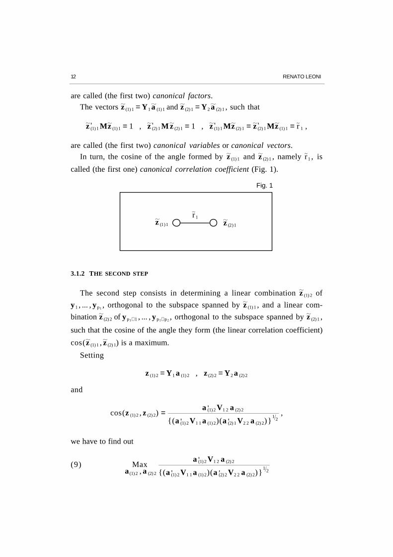
In turn, the cosine of the angle formed by z (1) 1 and z (2) 1 , namely r1 , is
called (the first one) canonical correlation coefficient (Fig. 1).
z (2)1z (1)1
Fig. 1
r1
3.1.2 THE SECOND STEP
The second step consists in determining a linear combination z (1) 2 of
y1 , ... , yp1, orthogonal to the subspace spanned by z (1) 1 , and a linear com-
bination z (2) 2 of yp1+ 1 , ... , yp1+ p2, orthogonal to the subspace spanned by z (2) 1 ,
such that the cosine of the angle they form (the linear correlation coefficient)
cos(z (1) 1 , z (2) 1) is a maximum.
Setting
z (1) 2 = Y1 a (1) 2 , z (2) 2 = Y2 a (2) 2
and
cos(z (1) 2 , z (2) 2) = a (1) 2' V1 2 a (2) 2
{(a (1) 2' V1 1 a (1) 2)(a (2) 1' V2 2 a (2) 2)}1
2 ,
we have to find out
(9) Max a (1) 2 , a (2) 2
a (1) 2' V1 2 a (2) 2
{(a (1) 2' V1 1 a (1) 2)(a (2) 2' V2 2 a (2) 2)}1
2

CANONICAL CORRELATION ANALYSIS 13
under the constraints
z (1) 2' M z (1) 1 = a (1) 2' Y 1' MY1a (1) 1 = a (1) 2' V1 1 a (1) 1 = 0
(10)
z (2) 2' M z (2) 1 = a (2) 2' Y2' MY2 a (2) 1 = a (2) 2' V2 2 a (2) 1 = 0 .
Equivalently, assuming that z (1) 2 and z (2) 2 are vectors of unitary square
length, we have to look for
(9') Max a (1) 2 , a (2) 2
a (1) 2' V1 2 a (2) 2 , a (1) 2' V1 1 a (1) 2 = 1 , a (2) 2' V2 2 a (2) 2 = 1
under the constraints in (10).
To solve the problem of constrained maximization set in (9') and (10),
consider the Lagrange function
L(a (1) 2 , a (2) 2 , κ 1 , κ 2 , κ 3 , κ 4) = a (1) 2' V1 2 a (2) 2 − 12
κ 1 (a (1) 2' V1 1 a (1) 2 − 1)
− 12
κ 2 (a (2) 2' V2 2 a (2) 2 − 1) − 12
κ 3 (a (1) 2' V1 1 a (1) 1) − 12
κ 4 (a (2) 2' V2 2 a (2) 1)
where κ 1 , κ 2 , κ 3 , κ 4 are Lagrange multipliers.
At (a (1) 1 , a (2) 1 , κ 1 , κ 2 , κ 3 , κ 4) where L(a (1) 2 , a (2) 2 , κ 1 , κ 2 , κ 3 , κ 4) has a
maximum, it must be
∂L∂a (1) 2
(a (1) 1 , a (2) 1 , κ 1 , κ 2 , κ 3 , κ 4)
= V1 2 a (2) 2 − κ 1 V1 1 a (1) 2 = 0
∂L∂a (2) 2
(a (1) 1 , a (2) 1 , κ 1 , κ 2 , κ 3 , κ 4)
= V2 1 a (1) 2 − κ 2 V2 2 a (2) 2 = 0
∂L∂κ 1
(a (1) 1 , a (2) 1 , κ 1 , κ 2 , κ 3 , κ 4)
= a (1) 2' V1 1 a (1) 2 = 1
∂L∂κ 2
(a (1) 1 , a (2) 1 , κ 1 , κ 2 , κ 3 , κ 4)
= a (2) 2' V2 2 a (2) 2 = 1
∂L∂κ 3
(a (1) 1 , a (2) 1 , κ 1 , κ 2 , κ 3 , κ 4)
= a (1) 2' V1 1 a (1) 1 = 0
∂L∂κ 4
(a (1) 1 , a (2) 1 , κ 1 , κ 2 , κ 3 , κ 4)
= a (2) 2' V2 2 a (2) 1 = 0

14 RENATO LEONI
from which we immediately deduce that
a (1) 2' V1 2 a (2) 2 = κ 1 , a (2) 2' V2 1 a (1) 2 = κ 2
and hence that
a (1) 2' V1 2 a (2) 2 = κ 1 = cos(z (1) 2 , z (2) 2) = κ 2 = a (2) 2' V2 1 a (1) 2 .
Therefore − since it must be
V1 2 a (2) 2 = cos(z (1) 2 , z (2) 2) V1 1 a (1) 2 , V2 1 a (1) 2 = cos(z (1) 2 , z (2) 2) V2 2 a (2) 2
a (1) 2' V1 1 a (1) 2 = 1 , a (2) 2' V2 2 a (2) 2 = 1
a (1) 2' V1 1 a (1) 1 = 0 , a (2) 2' V2 2 a (2) 1 = 0
− we realize that cos(z (1) 2 , z (2) 2) and a (1) 2 , a (2) 2 must be found among the
solutions of the system
(11) −r V1 1 V1 2
V2 1 −r V2 2
a (1) 2
a (2) 2 = 0 ,
a (1) 2' V1 1 a (1) 2 = 1 , a (2) 2' V2 2 a (2) 2 = 1
a (1) 2' V1 1 a (1) 1 = 0 , a (2) 2' V2 2 a (2) 1 = 0
in the unknowns r , a (1) 2 , a (2) 2 .
To this end, consider the system
(12)−r V1 1 V1 2
V2 1 −r V2 2
a (1) 2
a (2) 2 = 0
and ask for which values of r it admits non-trivial solutions with respect to
the unknowns a (1) 2 , a (2) 2 (7).
This system − similar to that one written in (3) − admits the solution r2
for the unknown r.
This solution can also be obtained as square root of the second largest
eigenvalue of the equation (5).
Now, consider the system
(7) On account of the constraints of normalization in (11), it is necessary to consider only the non-trivial solutions of the system (12).

CANONICAL CORRELATION ANALYSIS 15
(13) −r2 V1 1 V1 2
V2 1 −r2 V2 2
a (1) 2
a (2) 2 = 0 ,
a (1) 2' V1 1 a (1) 2 = 1 , a (2) 2' V2 2 a (2) 2 = 1
a (1) 2' V1 1 a (1) 1 = 0 , a (2) 2' V2 2 a (2) 1 = 0
in the unknowns a (1) 2 , a (2) 2 , obtained by setting r = r2 in (11).
Pay attention to the system represented by the first equation in (13),
namely
(13')−r2 V1 1 V1 2
V2 1 −r2 V2 2
a (1) 2
a (2) 2 = 0 .
Premultiplying both members of (13') by the matrix
(14)r2 I p 1
V1 2 V2 2-1
O (p 2 , p 1) (1 r2) V2 2-1
,
we get the system
(15) (− r 22 I p 1
+ V 1 1-1 V1 2 V2 2
-1 V2 1) a (1) 2 = 0 , a (2) 2 = 1 r2
V2 2-1 V2 1 a (1) 2
and, as the matrix (14) is nonsingular, the systems (13') and (15) are
equivalent.
Clearly, the first equation in (15) admits the eigenvector a (1) 2 such that
a (1) 2' V1 1 a (1) 2 = 1 and a (1) 2' V1 1 a (1) 1 = 0, corresponding to the eigenvalue r 22 .
In turn, the second equation in (15), for a (1) 2 = a (1) 2 , gives the vector
a (2) 2 = 1 r2
V2 2-1 V2 1 a (1) 2
such that a (2) 2' V2 2 a (2) 2 = 1 and a (2) 2' V2 2 a (2) 1 = 0.
In fact, taking into account that
{(− r 22 I p 1
+ V 1 1-1 V1 2 V2 2
-1 V2 1) a (1) 2 = 0} ⇔ {V1 1-1 V1 2 V2 2
-1 V2 1 a (1) 2 = r 22 a (1) 2}
⇔ {a (1) 2' V1 2 V2 2-1 V2 1 a (1) 2 = r 2
2} ,
we have

16 RENATO LEONI
a (2) 2' V2 2 a (2) 2 = 1 r 2
2 a (1) 2' V1 2 V2 2
-1 V2 2 V2 2-1 V2 1 a (1) 2 = 1
r22 a (1) 2' V1 2 V2 2
-1 V2 1 a (1) 2
= 1 r 2
2 r 2
2 = 1 .
Further, since V1 2 a (2) 1 = r 1 V1 1 a (1) 1 (Section 3.1.1), we get
a (2) 2' V2 2 a (2) 1 = 1 r2
a (1) 2' V1 2 V2 2-1 V2 2 a (2) 1 = 1
r2
a (1) 2' V1 2 a (2) 1
= r 1
r 2
a (1) 2' V1 1 a (1) 1 = 0 .
Thus, we immediately conclude that a (1) 2 , a (2) 2 , solutions of the system
(15) with the properties mentioned above, are also solutions of the system
(13).
Of course, a (1) 2 = a (1) 2 , a (2) 2 = a (2) 2 represent a solution of the problem set
in (9) and (10).
Finally, it can easily be shown that
a (1) 1' V1 2 a (2) 2 = a (2) 1' V2 1 a (1) 2 = 0 .
The vectors a (1) 2 and a (2) 2 , such that
a (1) 2' V1 1 a (1) 2 = 1 , a (2) 2' V2 2 a (2) 2 = 1 ,
a (1) 2' V1 1 a (1) 1 = a (2) 2' V2 2 a (2) 1 = 0 , a (1) 1' V1 2 a (2) 2 = a (2) 1' V2 1 a (1) 2 = 0 ,
a (1) 2' V1 2 a (2) 2 = a (2) 2' V2 1 a (1) 2 = r 2 ,
are called (the second two) canonical factors.
The vectors z (1) 2 = Y1 a (1) 2 and z (2) 2 = Y2 a (2) 2 , such that
z (1) 2' M z (1) 2 = 1 , z (2) 2' M z (2) 2 = 1 ,
z (1) 2' M z (1) 1 = z (2) 2' M z (2) 1 = 0 , z (1) 1' M z (2) 2 = z (2) 1' M z (1) 2 = 0 ,
z (1) 2' M z (2) 2 = z (2) 2' Mz (1) 2 = r 2 ,
are called (the second two) canonical variables or canonical vectors.
The cosine of the angle formed by z (1) 2 and z (2) 2 , namely r2 , is called (the

CANONICAL CORRELATION ANALYSIS 17
second one) canonical correlation coefficient (Fig. 2).
z (1)1 z (2)1
z (1)2 z (2)2r2
r1
Fig. 2
3.1.3 THE FOLLOWING STEPS
The procedure described in the preceding pages may be iterated for
s = 3 , ... , k.
At the sth step the problem lies in finding a linear combination z (1) s of
y1 , ... , yp1, orthogonal to the subspace spanned by z (1) 1 , ... , z (1) s -1 , and a
linear combination z (2) s of yp1+ 1 , ... , yp1+ p2, orthogonal to the subspace
spanned by z (2) 1 , ... , z (2) s -1 , such that the cosine of the angle they form (the
linear correlation coefficient) cos(z (1) s , z (2) s) is a maximum.
Setting
z (1) s = Y1 a (1) s , z (2) s = Y2 a (2) s
and
cos(z (1) s , z (2) s) = a (1) s' V1 2 a (2) s
{(a (1) s' V1 1 a (1) s)(a (2) s' V2 2 a (2) s)}1
2 ,
we have to find out
(16) Max a (1) s , a (2) s
a (1) s' V1 2 a (2) s
{(a (1) s' V1 1 a (1) s)(a (2) s' V2 2 a (2) s)}1
2
18 RENATO LEONI
under the constraints (3 ≤ s ≤ k; t = 1 , ... , s − 1)
z (1) s' M z (1) t = a (1) s' Y 1' MY1a (1) t = a (1) s' V1 1 a (1) t = 0
(17)
z (2) s' M z (2) t = a (2) s' Y2' MY2 a (2) t = a (2) s' V2 2 a (2) t = 0 .
Equivalently, assuming that z (1) s and z (2) s are vectors of unitary square
length, we have to look for
(16') Max a (1) s , a (2) s
a (1) s' V1 2 a (2) s , a (1) s' V1 1 a (1) s = 1 , a (2) s' V2 2 a (2) s = 1
under the constraints in (17).
Solving the problem of maximization set in (16') and (17) by the
Lagrange method − since at the maximum it must be (8)
V1 2 a (2) s = cos(z (1) s , z (2) s) V1 1 a (1) s , V2 1 a (1) s = cos(z (1) s , z (2) s) V2 2 a (2) s
a (1) s' V1 1 a (1) s = 1 , a (2) s' V2 2 a (2) s = 1
a (1) s' V1 1 a (1) t = 0 , a (2) s' V2 2 a (2) t = 0
− we realize that cos(z (1) s , z (2) s) and a (1) s , a (2) s has to be found among the
solutions of the system
(18) −r V1 1 V1 2
V2 1 −r V2 2
a (1) s
a (2) s = 0 ,
a (1) s' V1 1 a (1) s = 1 , a (2) s' V2 2 a (2) s = 1
a (1) s' V1 1 a (1) t = 0 , a (2) s' V2 2 a (2) t = 0
in the unknowns r , a (1) s , a (2) s .
To this end, consider the system
(19)−r V1 1 V1 2
V2 1 −r V2 2
a (1) s
a (2) s = 0
and ask for which values of r it admits non-trivial solutions with respect to
(8) Details are left to the reader.

CANONICAL CORRELATION ANALYSIS 19
the unknowns a (1) s , a (2) s (9).
This system − similar to that one written in (3) − admits the solution
rs > 0 for the unknown r.
This solution can also be obtained as square root of the sth largest
eigenvalue of the equation (5).
Now, consider the system
(20) −rs V1 1 V1 2
V2 1 −rs V2 2
a (1) s
a (2) s = 0 ,
a (1) s' V1 1 a (1) s = 1 , a (2) s' V2 2 a (2) s = 1
a (1) s' V1 1 a (1) t = 0 , a (2) s' V2 2 a (2) t = 0
in the unknowns a (1) s , a (2) s , obtained by setting r = r s in (18).
Pay attention to the system represented by the first equation in (20),
namely
(20')−rs V1 1 V1 2
V2 1 −rs V2 2
a (1) s
a (2) s = 0 .
Premultiplying both members of (20') by the matrix
(21)rs I p 1
V1 2 V2 2-1
O (p 2 , p 1) (1 rs) V2 2-1
,
we get the system
(22) (− r s2 I p 1
+ V 1 1-1 V1 2 V2 2
-1 V2 1) a (1) s = 0 , a (2) s = 1 r s
V2 2-1 V2 1 a (1) s
and, as the matrix (21) is nonsingular, the systems (20') and (22) are
equivalent.
Clearly, the first equation in (22) admits the eigenvector a (1) s such that
a (1) s' V1 1 a (1) s = 1 and a (1) s' V1 1 a (1) t = 0, corresponding to the eigenvalue r s2.
In turn, the second equation in (22), for a (1) s = a (1) s , gives the vector
(9) On account of the constraints of normalization in (17), it is necessary to consider only the non-trivial solutions of the system (19).

20 RENATO LEONI
a (2) s = 1 r s
V2 2-1 V2 1 a (1) s
such that a (2) s' V2 2 a (2) s = 1 and a (2) s' V2 2 a (2) t = 0.
Thus, we conclude that a (1) s , a (2) s , solutions of the system (22) with the
properties mentioned above, are also solutions of the system (20).
Of course, a (1) s = a (1) s , a (2) s = a (2) s represent a solution of the problem set
in (16) and (17).
Finally, it can easily be shown that
a (1) t' V1 2 a (2) s = a (2) t' V2 1 a (1) s = 0 .
The vectors a (1) s and a (2) s , such that
a (1) s' V1 1 a (1) s = 1 , a (2) s' V2 2 a (2) s = 1 ,
a (1) s' V1 1 a (1) t = a (2) s' V2 2 a (2) t = 0 , a (1) t' V1 2 a (2) s = a (2) t' V2 1 a (1) s = 0 ,
a (1) s' V1 2 a (2) s = a (2) s' V2 1 a (1) s = r s ,
are called (the sth two) canonical factors.
The vectors z (1) s = Y1 a (1) s and z (2) s = Y2 a (2) s , such that
z (1) s' M z (1) s = 1 , z (2) s' M z (2) s = 1 ,
z (1) s' M z (1) t = z (2) s' M z (2) t = 0 , z (1) t' M z (2) s = z (2) t' M z (1) s = 0 ,
z (1) s' Mz (2) s = z (2) s' Mz (1) s = r s ,
are called (the sth two) canonical variables or canonical vectors.
The cosine of the angle formed by z (1) s and z (2) s , namely rs , is called (the
sth one) canonical correlation coefficient.
3.2 FUNDAMENTAL PROPERTIES OF CCA
Writing
A (1) = a (1) 1 a (1) k , A (2) = a (2) 1 a (2) k , R = diag (r1 , ... , rk)
and

CANONICAL CORRELATION ANALYSIS 21
Z (1) = z (1) 1 z (1) k = Y1 A (1) , Z (2) = z (2) 1 z (2) k = Y2A (2) ,
some fundamental properties of CCA can be pointed out.
1. We have
(23) Z (1)' MZ (1) = A (1)' V1 1 A (1) = I k , Z (2)' MZ (2) = A (2)' V2 2 A (2) = I k .
In other words, the canonical variables z (1) 1 , ... , z (1) k of the first set are
uncorrelated and with unitary variance; the same is true for the canonical
variables z (2) 1 , ... , z (2) k of the second set.
2. We have
(24) Z (1)' MZ (2) = A (1)' V1 2 A (2) = R .
Namely, each canonical variable of the first set presents correlation rh > 0
(h = 1 , ... , k) with the corresponding canonical variable of the second set,
while each of the remaining canonical variables of the first set is uncorre-
lated with each of the remaining canonical variables of the second set.
REMARK 1. Since canonical variables and canonical correlation coefficients
are, as can easily be shown, invariant with respect to scale changes, CCA
is very often performed after standardization of each original variable, which
leads us to work with correlation matrices rather than with covariance ma-
trices.
REMARK 2. In order to compute the canonical correlation coefficients
r1 , ... , rk , instead of the equation
(i) det(− r2 I p 1 + V 1 1
-1 V1 2 V2 2-1 V2 1) = 0 ,
we could employ the equation
(ii) det(− r2 I p 2 + V 2 2
-1 V2 1 V1 1-1 V1 2) = 0
where V2 2-1 V2 1 V1 1
-1 V1 2 may be interpreted as the matrix of a selfadjoint
22 RENATO LEONI
transformation in the metric represented by V2 2 ((V 2 2-1 V2 1 V1 1
-1 V1 2)'V2 2 =
V2 1 V1 1-1 V1 2 = V 2 2 (V 2 2
-1 V2 1 V1 1-1 V1 2)).
Analogously, to the end of computing the canonical factors a (1) 1 , ... , a (1) k
and a (2) 1 , ... , a (2) k , instead of the equations (h = 1 , ... , k)
(iii) (− r h2 I p 1
+ V 1 1-1 V1 2 V2 2
-1 V2 1) a (1) h = 0 , a (2) h = 1 rh
V2 2-1 V2 1 a (1) h .
we could employ the equations (h = 1 , ... , k)
(iv) (− r h2 I p 2
+ V 2 2-1 V2 1 V1 1
-1 V1 2) a (2) h = 0 , a (2) h = 1 rh
V1 1-1 V1 2 a (2) h .
However, from the computation point of view, employing (ii) and (iv)
instead of (i) and (iii) is the same if p1 = p2 , and is not convenient if
p1 < p2 .
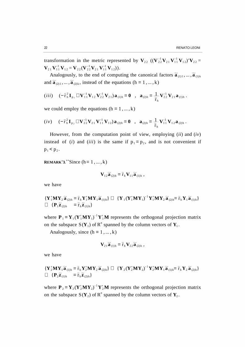
REMARK 3. Since (h = 1 , ... , k)
V1 2 a (2) h = rh V1 1 a (1) h ,
we have
{Y 1' MY2 a (2) h = rh Y1' MY1 a (1) h} ⇔ {Y 1 (Y1' MY1)- 1 Y1' MY2 a (2) h= rh Y1 a (1) h}
⇔ {P1 z (2) h = rh z (1) h}
where P 1 = Y1 (Y 1' MY1)- 1 Y 1' M represents the orthogonal projection matrix
on the subspace S(Y1) of Rn spanned by the column vectors of Y1 .
Analogously, since (h = 1 , ... , k)
V2 1 a (1) h = rh V2 2 a (2) h ,
we have
{Y 2' MY1 a (1) h = rh Y2' MY2 a (2) h} ⇔ {Y 2 (Y2' MY2)- 1 Y2' MY1 a (1) h= rh Y2 a (2) h}
⇔ {P2 z (1) h = rh z (2) h}
where P 2 = Y2 (Y 2' MY2)- 1 Y 2' M represents the orthogonal projection matrix
on the subspace S(Y2) of Rn spanned by the column vectors of Y2 .

CANONICAL CORRELATION ANALYSIS 23
Hence, the orthogonal projection of z (2) h on S(Y1) is homothetic with z (1) h
and, similarly, the orthogonal projection of z (1) h on S(Y2) is homothetic with
z (2) h (Fig. 3).
Fig. 3
z (1)h
z (2)hP2 z (1)h
P1 z (2)h
REMARK 4. Taking into account what was mentioned above, is immediately
apparent that we can write
P 1 P 2 z (1) h = r h2 z (1) h , P2 P 1 z (2) h = r h
2 z (2) h .
Thus, square canonical correlation coefficients and canonical variables
may also be interpreted as eigenvalues and eigenvectors of the linear
transformations corresponding to the matrices P 1 P 2 and P 2 P 1 (10).
REMARK 5. Some particular aspects of CCA should be noticed.
a. If p1 = 1 = p2 , the equation (5) can be written as
det (− r2 + σ1 22
σ 12 σ 2
2) = 0 .
Then,
r12 = σ1 2
2
σ 12 σ 2
2 ,
(10) As can easily be verified, the restrictions of these linear transformations, respectively, toS(Y1) and S(Y2) are selfadjoint.

24 RENATO LEONI
the square linear correlation coefficient between the variables y1 and y2 .
b. If p1 = 1 and p2 > 1, the equation (5) can be written as
det (− r 2 + V1 2 V2 2-1 V2 1
σ 12
) = 0 .
Then,
r12 = V1 2 V2 2
-1 V2 1
σ 12
,
the square multiple linear correlation coefficient between the variables y1
and y2 , ... , y1+ p2.
c. Denote by ρ(z (1) h , Y2) (h = 1 , ... , k) the square multiple linear correlation
coefficient between the variables z (1) h = Y1 a (1) h and yp1+ 1 , ... , yp1+ p2.
Moreover, denote by
z (1) h , Y2 = Y2 (Y 2' MY2)
- 1 Y 2' MY1 a (1) h
the orthogonal projection of z (1) h on the subspace spanned by the variables
yp1+ 1 , ... , yp1+ p2.
Then, as can easily be verified, it results
ρ(z (1) h , Y2) = cos2 ( z (1) h , z (1) h , Y2) = a (1) h' V1 2 V2 2
-1 V2 1 a (1) h = rh2 .
Analogously, denote by ρ(z (2) h , Y1) (h = 1 , ... , k) the square multiple
linear correlation coefficient between the variables z (2) h = Y2 a (2) h and
y1 , ... , yp1.
Moreover, denote by
z (2) h , Y1 = Y1 (Y 1' MY1)
- 1 Y 1' MY2 a (2) h
the orthogonal projection of z (2) h on the subspace spanned by the variables
y1 , ... , yp1.
Then, it results
ρ(z (2) h , Y1) = cos2 ( z (2) h , z (2) h , Y1) = a (2) h' V2 1 V1 1
-1 V1 2 a (2) h = rh2 .

CANONICAL CORRELATION ANALYSIS 25
REMARK 6. Assuming that k < p1 ≤ p2 , the k canonical variables
z (1) 1 , ... , z (1) k
form an orthonormal basis of a (proper) subspace of the space S(Y1) (of
dimension p1) spanned by the column vectors of Y1 and, analogously, the k
canonical variables
z (2) 1 , ... , z (2) k
form an orthonormal basis of a (proper) subspace of the space S(Y2) (of
dimension p2) spanned by the column vectors of Y2 .
In order to complete these bases, we can proceed as follows.
Firstly, find p1 − k canonical factors a (1) k+ 1 , ... , a (1) p1 and p2 − k canon-
ical factors a (2) k+ 1 , ... , a (2) p2 − which are solutions, respectively, of the
equations (u = k +1 , ... , p1 ; v = k +1 , ... , p2)
V2 1 a (1) u = 0 or (V 1 1-1 V1 2 V2 2
-1 V2 1) a (1) u = 0
and
V1 2 a (2) v = 0 or (V 2 2-1 V2 1 V1 1
-1 V1 2) a (2) v = 0
− such that, setting
A(1) + = a (1) k +1 a (1) p1 , A(2) + = a (2) k + 1 a (2) p2
,
we have (I , O of appropriate order)
A(1) +' V1 1 A(1) + = I , A(2) +' V2 2 A(2) + = I
A(1)' V1 2 A(2) + = O , A(2)
' V2 1 A(1) + = O
A(2) +' V2 1 A(1) + = O , A(1)' V1 1 A(1) + = O
A(2)' V2 2 A(2) + = O .
Successively, define p1 − k canonical variables
z (1) k+ 1 = Y1 a (1) k+ 1 , ... , z (1) p1 = Y1 a (1) p1

26 RENATO LEONI
and p2 − k canonical variables
z (2) k+ 1 = Y2 a (2) k+ 1 , ... , z (2) p2 = Y2 a (2) p2
such that, setting
Z (1) + = z (1) k+ 1 z (1) p1 , Z (2) + = z (2) k+ 1 z (2) p2
,
we have (I , O of appropriate order)
Z (1) +' M Z (1) + = I , Z (2) +' M Z (2) + = I
Z (1)' M Z (2) + = O , Z (2)
' M Z (1) + = O
Z (2) +' M Z (1) + = O , Z (1)' M Z (1) + = O
Z (2)' M Z (2) + = O .
Notice that, writing
A(1) + + = A(1) A(1) + , A(2) + + = A(2) A(2) + ,
Z (1) + + = Z (1) Z (1) + , Z (2) + + = Z (2) Z (2) + ,
it results (I , O of appropriate order)
A(1) + +' V1 1 A(1) + + = I , A(2) + +' V2 2 A(2) + + = I
A(1) + +' V1 2 A(2) + + = diag(R , O)
and
Z (1) + +' M Z (1) + + = I , Z (2) + +' M Z (2) + + = I
Z (1) + +' M Z (2) + + = diag(R , O) .
REMARK 7. As can easily be verified, from the relations
Z (1) + + = Y1 A(1) + + , Z (2) + + = Y2 A(2) + + ,
we get the so-called reconstitution formulas
Y1 = Z (1)A(1)' V1 1 + Z (1) +A(1) +' V1 1 , Y2 = Z (2)A(2)
' V2 2 + Z (2) +A(2) +' V2 2 .

CANONICAL CORRELATION ANALYSIS 27
4 GRAPHICAL REPRESENTATION OF VARIABLES
AND INDIVIDUALS
4.1 GRAPHICAL REPRESENTATION OF VARIABLES
A graphical representation of the p variables y1 , ... , yp (measured in
terms of deviations from the means) is usually obtained by their orthogonal
projections on the subspace spanned by the first canonical variable
(canonical axis) or the first two canonical variables (canonical plane),
belonging to S(Y1) or S(Y2).
In S(Y1), for example, the orthogonal projection y j of y j (j = 1, ... , p) on
the canonical plane S (z (1) 1 , z (1) 2) is given by
y j = z (1) 1 z (1) 1' M y j + z (1) 2 z (1) 2' M y j = z (1) 1 σ j r1 j + z (1) 2 σ j r2 j
where r1 j and r2 j denote, respectively, the linear correlation coefficients of
z (1) 1 and z (1) 2 with y j .
However, since we are mainly interested in representing linear correla-
tions between pairs of variables or between a variable and a canonical
variable, it is more suitable to work with standardized variables.
In that case, the orthogonal projection y j* of the standardized variable
y j* = y j σ j (j = 1, ... , p) on the canonical plane S (z (1) 1 , z (1) 2) is given by
y j* = z (1) 1 z (1) 1' M y j
* + z (1) 2 z (1) 2' M y j* = z (1) 1 r1 j + z (1) 2 r2 j .
Thus, the co-ordinates of y j* relative to z (1) 1 , z (1) 2 are (r1 j , r2 j) (Fig. 4).
Of course, each y j* (j = 1, ... , p) lies inside a circle of centre 0 and radius 1
(the so-called correlation circle).
Moreover, the quality of representation of y j* on S (z (1) 1 , z (1) 2) can be
judged by means of the square cosine of the angle formed by y j* and y j
*
which is given by ((y j*)'M(y j
*) = 1)
QR(j ; z (1) 1 , z (1) 2) = [(y j
*)'M( y j*)]2
[(y j*)'M(y j
*) ] [ (y j*)'M( y j
*) ] =
[(y j*)'M( y j
*)]2
( y j*)'M( y j
*) .

28 RENATO LEONI
y j*
r1 j
r2 j
Fig. 4
0z (1)1
z (1)2
l
ll
l
l
A high QR(j ; z (1) 1 , z (1) 2) − for example, QR(j ; z (1) 1 , z (1) 2) ≥ 0.7 − means
that y j* is well represented by y j
* ; on the contrary, a low QR(j ; z (1) 1 , z (1) 2)
means that the representation of y j* by y j
* is poor.
Notice that another expression of QR(j ; z (1) 1 , z (1) 2) may be obtained
taking into account that
(y j*)'M( y j
*) = (y j*)'M(z (1) 1 r1 j + z (1) 2 r2 j) = r1 j
2 + r2 j2
and
( y j*)'M( y j
*) = (z (1) 1 r1 j + z (1) 2 r2 j)'M(z (1) 1 r1 j + z (1) 2 r2 j) = r1 j2 + r2 j
2 .
Thus,
QR(j ; z (1) 1 , z (1) 2) = r1 j2 + r2 j
2 .
On the other hand, since QR(j ; z (1) 1 , z (1) 2) also denotes the square
distance of y j* from the correlation circle centre, we can see that well-
represented variables lie near the circumference of the correlation circle.
Concluding, for well-represented variables we can visualize on the corre-
lation circle:

CANONICAL CORRELATION ANALYSIS 29
• which variables are correlated among themselves and with each
canonical variable;
• which variables are uncorrelated (orthogonal) among themselves and
with each canonical variable.
Of course, an analogous representation may be carried out on the can-
onical plane S (z (2) 1 , z (2) 2) .
These two representations refer to different ways of visualization and are
very similar provided that the canonical correlation coefficients between
each pair of corresponding canonical variables are close to 1.
4.2 GRAPHICAL REPRESENTATION OF INDIVIDUALS
Now, let us consider the n column vectors (individuals) y (1) 1 , ... , y (1) n of
Y1' and the n column vectors (individuals) y (2) 1 , ... , y (2) n of Y2' .
Suppose that these vectors belong, respectively, to the vector spaces Rp1
and Rp2.
Moreover, assume that V1 1-1 and V2 2
-1 are the matrices of the scalar
product in Rp1 and Rp2, relative to their corresponding canonical bases.
Setting (h = 1 , ... , k)
c(1) h = V 1 1 a (1) h , c(2) h = V 2 2 a (2) h
it is immediately apparent that
[c(1) 1 c(1) k ]'V1 1-1 [c(1) 1 c(1) k ]= I k , [c(2) 1 c(2) k ]'V2 2
-1 [c(2) 1 c(2) k ]= I k .
In Rp1, a graphical representation of the n individuals y (1) 1 , ... , y (1) n is
usually obtained by their orthogonal projections on the subspace S (c(1) 1)
spanned by c(1) 1 or on the subspace S (c(1) 1 , c(1) 2) spanned by c(1) 1 , c(1) 2 .
Confining ourselves to considering this last type of representation, we
notice that the orthogonal projection y (1) i of y (1) i (i = 1 , ... , n) on S (c(1) 1 , c(1) 2)
is given by

30 RENATO LEONI
y (1) i = [c(1) 1 c(1) 2 ][c(1) 1 c(1) 2 ]'V1 1-1 y (1) i
= c(1) 1 c(1) 1' V1 1-1 y (1) i + c(1) 2 c(1) 2' V1 1
-1 y (1) i
= c(1) 1 a (1) 1' y (1) i + c(1) 2 a (1) 2' y (1) i
= c(1) 1 z i 1 + c(1) 2 z i 2
where z i j (j = 1 , 2) is the ith element of the canonical vector z (1) j .
Thus, the co-ordinates of y (1) i relative to c(1) 1 , c(1) 2 are (z i 1 , z i 2) (Fig. 5).
Fig. 5
0
y (1)i
z i 1
z i 2
c(1)1
c(1)2
l
l
l
l
l
Moreover, the quality of representation of each y (1) i (i = 1 , ... , n) on
S (c(1) 1 , c(1) 2) can be judged by means of the square cosine of the angle
formed by y (1) i and y (1) i which is given by
QR(i ; c(1) 1 , c(1) 2) = (y (1) i' V1 1
-1 y (1) i)2
(y (1) i' V1 1-1 y (1) i) (y (1) i' V1 1
-1 y (1) i) .
A high QR(i ; c(1) 1 , c(1) 2) − for example, QR(i ; c(1) 1 , c(1) 2) ≥ 0.7 − means
that y (1) i is well represented by y (1) i ; on the contrary, a low QR(i ; c(1) 1 , c(1) 2)
means that the representation of y (1) i by y (1) i is poor.
Of course, the procedure described above may be applied for the
representation of y (2) 1 , ... , y (2) n on the subspace S (c(2) 1 , c(2) 2) spanned by
c(2) 1 , c(2) 2 .

CANONICAL CORRELATION ANALYSIS 31
5 OTHER APPROACHES TO CCA
5.1 THE APPROACH IN TERMS OF THE MULTIVARIABLE LINEAR MODEL
The approach we would like to mention is based on the multivariable
linear model.
Firstly, consider the model
Y1 = Y2H 2 + E 2
where E2 is a matrix of «residuals» and H 2 is a matrix, of order (p2 , p1), of
unknown coefficients.
In order to determine the matrix H 2 , we can choose a least square
criterion.
However, without any assumption regarding the rank of H 2 , the best
solution is trivially given by
H 2 = (Y2' MY2) -1 Y2' MY1
where r (H 2) ≤ p1 = r (Y1) .
Then, assume that H 2 has rank k* < p 1 , so that it may be written in the
form (F2 and G2 of order, respectively, (p2 , k*) and (k* , p1))
H 2 = F2 G2
where r(F2) = r(G 2) = k*.
In this case, our model becomes
Y1 = Y2 F2 G2 + E 2
and we propose to find out
(25) Min tr {(Y1 − Y2 F2 G2)'M(Y1 − Y2 F2 G2) V1 1-1 } , F2' V2 2 F2 = I k * .
F2 , G2
To this end, first notice that, taking into account the constraint on the
matrix F2 , we can write

32 RENATO LEONI
tr {(Y1 − Y2F2 G2)'M(Y1 − Y2F2 G2) V1 1-1 }
= tr {Y1' MY1V1 1-1 } − tr {Y1' MY2F2 G2 V1 1
-1 }
− tr {G2' F2' Y2' MY1V1 1-1 } + tr {G2' F2' Y2' MY2 F2 G2 V1 1
-1 }
= tr {I k *} − 2 tr {V1 2 F2 G2 V1 1-1 } + tr {G2' G2 V1 1
-1 } .
Thus, our problem lies in finding out
(25') Max {2 tr {V1 2 F2 G2 V1 1-1 } − tr {G2' G2 V1 1
-1 }} , F2' V2 2 F2 = I k ∗ .F2 , G2
Now, consider the function
L(F 2 ,G2 ,L2) = 2tr {V1 2 F2 G2 V1 1-1 } − tr {G2' G2 V1 1
-1 }} − tr {(F2' V2 2 F2 − Ik *) L2}
where L2 = L 2' is a matrix of Lagrange multipliers of order (k* , k*).
At (F2 ,G2 , L2) where L(F 2 ,G2 ,L2) has a maximum, as can easily be
verified, it must be
V2 1 V1 1-1 G2
' = V2 2 F2 L2
F2' V2 1 = G2
F2' V2 2 F2 = I k * .
Therefore, we must find out solutions of the system
V2 1 V1 1-1 G2' = V2 2 F2 L2
F2' V2 1 = G 2
F2' V2 2 F2 = I k *
in the unknowns F2 , G2 , L2 .
Clearly,
F2 = A(2)* = a (2) 1 a (2) k * , G2 = (A(2)
* )' V2 1 , L2 = (R*) 2 = diag (r 12 , ... , r k *
2 )
is a solution of our problem.
Successively, consider the model
Y2 = Y1H 1 + E 1
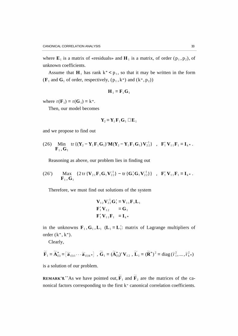
CANONICAL CORRELATION ANALYSIS 33
where E1 is a matrix of «residuals» and H 1 is a matrix, of order (p1 , p2), of
unknown coefficients.
Assume that H 1 has rank k* < p 1 , so that it may be written in the form
(F1 and G1 of order, respectively, (p1 , k*) and (k* , p2))
H 1 = F1 G1
where r(F1) = r(G 1) = k*.
Then, our model becomes
Y2 = Y1 F1 G1 + E 1
and we propose to find out
(26) Min tr {(Y2 − Y1 F1 G1)'M(Y2 − Y1 F1 G1) V2 2-1 } , F1' V1 1 F1 = I k * .
F1 , G1
Reasoning as above, our problem lies in finding out
(26') Max {2 tr {V2 1 F1 G1 V2 2-1 } − tr {G1' G1 V2 2
-1 }} , F1' V1 1 F1 = I k * .F1 , G1
Therefore, we must find out solutions of the system
V1 2 V2 2-1 G1' = V1 1 F1 L1
F1' V1 2 = G 1
F1' V1 1 F1 = I k *
in the unknowns F1 , G1 , L1 (L1 = L 1': matrix of Lagrange multipliers of
order (k* , k*).
Clearly,
F1 = A(1)* = a (1) 1 a (1) k * , G1 = (A(1)
* )' V1 2 , L1 = (R*) 2 = diag (r 12 , ... , r k *
2 )
is a solution of our problem.
REMARK 8. As we have pointed out, F1 and F2 are the matrices of the ca-
nonical factors corresponding to the first k* canonical correlation coefficients.

34 RENATO LEONI
In turn, G1 and G2 − taking into account that Z (1)* = Y1F1 and Z (2)
* = Y2F2
are the matrices of the first k* canonical variables − can be interpreted as
the matrices of the orthogonal projection coefficients of Y1 and Y2 on the sub-
spaces spanned by those canonical variables.
REMARK 9. Notice the relations
F1 = V 1 1-1 V1 2 F2 (R*)- 1 = V 1 1
-1 G2' (R*)- 1 , F2 = V 2 2
-1 V2 1 F1 (R*)- 1 = V 2 2-1 G1
' (R*)- 1 .
Alternatively, consider the model
Y1A1 = Y2A2 + E 3
where E3 is a matrix of «residuals», A1 and A2 are matrices of unknown
coefficients of order, respectively, (p1 , k*) and (p2 , k*), such that r(A 1) =r(A 2) = k* .
We propose to find out
(27) Min tr {(Y1A1 − Y2A2)'M(Y1A1 − Y2A2)} , A 1' V1 1 A1 = I k * .A1 , A2
To this end, first notice that, taking into account the constraint on the
matrix A1 , our problem lies in finding out
(27') Max 2 tr {A1' V1 2 A2} − tr {A2' V2 2 A2} , A1' V1 1 A1 = I k * .A1 , A2
Now, consider the function
L(A 1,A2 ,L3) = 2tr {A1' V1 2 A2} − tr {A2' V2 2 A2}} − tr {(A 1' V1 1 A(1) − Ik *) L3}
where L3 = L 3' is a matrix of Lagrange multipliers of order (k* , k*).
At (A1,A2 , L3) where L(A 1,A2 ,L3) has a maximum, it must be
V1 2 A2 = V1 1 A1 L3
V2 1 A1 = V2 2 A2
A1' V1 1 A1 = I k * .

CANONICAL CORRELATION ANALYSIS 35
Therefore, we must find out solutions of the system
V1 2 A2 = V1 1 A1 L3
V2 1 A1 = V2 2 A2
A1' V1 1 A1 = I k *
in the unknowns A1,A2 ,L3 .
Clearly,
A1 = F1 , A2 = F2 R* , L3 = (R*) 2
is a solution of our problem.
Analogously, consider the model
Y2B2 = Y1B1 + E 4
where E4 is a matrix of «residuals», B2 and B1 are matrices of unknown
coefficients of order, respectively, (p2 , k*) and (p1 , k*), such that r(B 2) =r(B 1) = k* .
It can easily be shown that
B2 = F2 , B1 = F1 R* .
REMARK 10. Notice that
B1 = A1 R* , B2 = A2 (R*)- 1 .
5.2 THE APPROACH IN TERMS OF PCA
Consider again the fundamental equation of CCA, namely the equation
−r V1 1 V1 2 V2 1 −r V2 2
a (1)
a (2) = 0 .
Setting
−r = 1 − λ ,
we can write (Q = diag (V 1 1-1 , V2 2
-1 ); O of appropriate order)

36 RENATO LEONI
{(1 − λ) V1 1 V1 2
V2 1 (1 − λ) V2 2
a (1)
a (2) = 0}
⇔ {( V1 1 V1 2 V2 1 V2 2
− λ V1 1 O O λ V2 2
) a (1)
a (2) = 0}
⇔ {( V1 1 V1 2 V2 1 V2 2
V1 1
-1 OO V2 2
-1 − λ I p )
V1 1 OO V2 2
a (1)
a (2) = 0}
⇔ {(VQ − λ I p) Q-1
a (1)
a (2) = 0}
⇔ {(VQ − λ I p) Q-1
a (1)
a (2) 1
2 = 0} .
Thus, the canonical correlation coefficients and the canonical factors are
linked to the eigenvalues and to the eigenvectors (appropriately norma-
lized) of the fundamental equation of PCA
(VQ − λ Ip) c = 0 ,
by means of the relations (h = 1 , ... , k)
−rh = 1 − λ h , a (1) h
a (2) h
= 2 Q ch .
Moreover, as is easily seen − for 0 < rh ≤ 1, namely for 1 < λ h ≤ 2 − the
principal component yh is linked to the canonical variables z (1) h , z (2) h by
means of the formula
(28) yh = Y1 Y2 Q ch = Y1 Y2 a (1) h
a (2) h
12
= z (1) h 12
+ z (2) h 12
.
Finally, since
(29) P1 yh = P1 z (1) h 12
+ P1 z (2) h 12
= z (1) h 12
+ rh z (1) h 12
= z (1) h 12
+ (λ h − 1) z (1) h 12
= z (1) h 12
+ λ h z (1) h 12
− z (1) h 12
= λ h z (1) h 12
and, analogously,

CANONICAL CORRELATION ANALYSIS 37
(30) P2 yh = λ h z (2) h 12
we also find that
(31) (P1 + P2) yh = λ h z (1) h 12
+ λ h z (2) h 12
= λ h (z (1) h 12
+ z (2) h 12
)
= λ h yh .
In other words, yh is an eigenvector of the matrix (P1 + P2) corresponding
to the eigenvalue λ h (11).
REMARK 11. Notice that from (29) and (30) we get the relations
z (1) h = 2 P1 yh
λ h
, z (2) h = 2 P2 yh
λ h
.
REMARK 12. Whenever n > p1 + p2 = p, as often happens in practical applica-
tions, it is not convenient, from the computation point of view, to use the
equation (P1 + P2)y = λ y to obtain first the eigenvalues λ 1 , ... , λ k and the
principal components y1 , ... , yk , then the canonical variables z (1) 1 , z (2) 1 , ... ,
z (1) k , z (2) k .
Rather, it is more suitable to perform a PCA to obtain first the eigen-
values and the principal components, then the canonical variables.
It is important to point out the statistical criterion underlying (31).
To this end, suppose we want to find a normalized linear combination y (1)
of y1 , ... , yp maximizing the sum of square multiple linear correlation coeffi-
cients ρ 1 + ρ2 between y (1) and the column vectors of Y1 and Y2 .
Denote by y a generic normalized linear combination of y1 , ... , yp .
Since we have (y 'M y = 1)
ρ 1 = cos2( y , P1 y) = y ' M P1 y , ρ2 = cos2( y , P2 y) = y ' M P2 y ,
(11) As can easily be verified, the linear transformation associated to (P1 + P2) is selfadjoint.

38 RENATO LEONI
we must find out
Max (ρ 1 + ρ 2) = Max (y'M(P1 + P 2)y ) , y'My = 1 .
y y
This problem of constrained maximization can be solved very easily.
It results that y (1) is given by the normalized eigenvector of (P1 + P2)
associated with the eigenvalue λ 1 .
In other words, y (1) = y1 , the first standardized principal component.
Of course, an analogous meaning may be attributed to each of the sub-
sequent standardized principal components.

CANONICAL CORRELATION ANALYSIS 39
REFERENCES
[l] Anderson, T.W., Introduction to Multivariate Statistical Analysis,
John Wiley and Sons, New York, 1958.
[2] Basilevsky, A., Statistical Factor Analysis and Related Methods,
John Wiley and Sons, New York, 1994.
[3] Bertier, P., Bouroche, J.M., Analyse des données multidimension-
nelles, PUF, Paris, 1977.
[4] Bouroche, J.M., Saporta, G., L'analisi dei dati, CLU, Napoli, 1983.
[5] Cailliez, F., Pages, G.P., Introduction à l'analyse des données,
Smash, Paris, 1976.
[6] Carroll, J.D., A Generalization of Canonical Correlation to Three
or More Sets of Variables, Proc. 76th Conv. Amer. Psych. Ass.,
1968.
[7] Coppi, R., Appunti di statistica metodologica: analisi lineare dei
dati, Dipartimento di Statistica, Probabilità e Statistiche Applicate,
Roma, 1986.
[8] Delvecchio, F., Analisi statistica di dati multidimensionali, Cacuc-
ci Editore, Bari, 1992.
[9] Diday, E., Lemaire, J., Pouget, J., Testu, F., Eléments d'analyse des
données, Dunod, Paris, 1982.
[10] Fabbris, L., Analisi esplorativa di dati multidimensionali, cleup
editore, Padova, 1990.
[11] Kettenring, R.J., Canonical Analysis of Several Sets of Variables,
Biometrika, 1971.
[12] Krzanowski, W.J., Principles of Multivariate Analysis, Oxford
University Press, Oxford, 2000.

40 RENATO LEONI
[13] Kshirsagar, A.M., Multivariate Analysis, Marcel Dekker, Inc.,
New York, 1972.
[14] Leoni, R., Alcuni argomenti di analisi statistica multivariata,
Dipartimento Statistico, Firenze, 1978.
[15] Leoni, R., Canonical Correlation Analysis, in «Methods for Multi-
dimensional Data Analysis», European Courses in Advanced
Statistics, Anacapri, 1987.
[16] Leoni, R., Modello lineare multivariato e analisi statistica mul-
tidimensionale, in «Conferenze di statistica nell'anno del 750°anniversario dell'Università degli Studi di Siena», Dipartimento di
Metodi Quantitativi, Siena, 1994.
[17] Leoni, R., Algebra lineare per le applicazioni statistiche,
Dipartimento di Statistica "G. Parenti", Firenze, 2007 (sta in
<http://www.ds.unifi.it> alla voce Materiale Didattico).
[18] Leoni, R., Principal Component Analysis, Department of Statistics
"G. Parenti", Florence, 2007.
[19] Mardia, K.V., Kent, I.T., Bibby, J.M., Multivariate Analysis,
Academic Press, London, 1979.
[20] Rizzi, A., Analisi dei dati, NIS, Roma, 1985.
[21] Saporta, G., Probabilités, Analyse des données et Statistique, E di-
tions Technip, Paris, 1990.
[22] Seber, G.A.F., Multivariate Observations, John Wiley and Sons,
New York, 1984.
[23] Volle, M., Analyse des données, Economica, Paris, 1981.