ALMA MATER STUDIORUM

UNIVERSITA' DI BOLOGNA

SCUOLA DI SCIENZE

Corso di laurea magistrale in Biologia Marina

Prokaryotic community structure in ultra-slow

spreading Southwest Indian Ridge

Tesi di laurea in

Microbiologia Marina e Cicli Biogeochimici

Relatore Presentata da

Prof. Roberto Borghese Gilda Varliero

Correlatore

Massimiliano Molari

II sessione

Anno Accademico 2014/2015

Contents

1. Introduction ......................................................................................................... 5

1.1 Deep sea ecosystems ................................................................................ 5

1.2 Hydrothermal systems and life ................................................................... 6

1.3 Ridge Systems ........................................................................................... 7

1.4 South West Indian Ridge ..........................................................................12

2. Objectives ..........................................................................................................14

3. Materials and Methods .......................................................................................15

3.1 Sample collection ......................................................................................15

3.2 Area Characterisation ...............................................................................16

3.3 DNA Extraction..........................................................................................18

3.4 DNA Sequencing.......................................................................................23

3.5 Statistical analysis .....................................................................................25

3.6 Phylogenetic Tree’s Construction..............................................................27

4. Results ...............................................................................................................29

4.1 Bacterial Diversity .....................................................................................29

4.1.1 Comparison between surface and subsurface .............................29

4.1.2 Comparison between areas: surface ...........................................32

4.1.3 Comparison between areas: subsurface .....................................33

4.2 Bacterial Community Composition ............................................................33

4.2.1 Subsurface ..................................................................................34

4.2.2 Surface ........................................................................................37

4.3 Archaeal Diversity .....................................................................................40

4.3.1 Comparison between surface and subsurface .............................40

4.3.2 Comparison between areas: surface ...........................................40

4.3.3 Comparison between areas: subsurface .....................................41

4.4 Archaeal Community Composition ............................................................41

4.4.1 Surface and subsurface ...............................................................42

5. Discussion ..........................................................................................................53

6. Conclusions ........................................................................................................64

7. Supplementary materials ....................................................................................65

7.1 Figures ......................................................................................................65

7.2 Tables .......................................................................................................66

8. Bibliography .......................................................................................................69

5

1. Introduction

1.1 Deep sea ecosystems

Deep-sea ecosystem extends from the continental shelf, about 200 m depth, to

the abyssal environments, of which the deepest point is the Mariana Trench

(11000 m; Danovaro et al., 2014). This ecosystem includes about 95% of seafloor

and about 67% of the Earth’s lithosphere (Jørgensen and Boetius et al., 2007).

Here, the average depth is about 4000 m, the average temperature is below than

4 °C and the average hydrostatic pressure is about 400 atm (Danovaro et al.,

2014). Sunlight penetrates maximum up to 300 m of the water column, so the

deep sea is in the dark and no photosynthesis occurs here (Orcutt et al., 2011),

and therefore the dominant biological process is respiration. About 1-40% of the

photosynthetic fixed carbon in the euphotic zone is exported in dark deep sea

(Herndl et al., 2013), but only 0,4% of primary production is buried in oceanic

sediment, due to efficiently removal of organic matter by pelagic heterotrophic

microorganisms (Middelburg et al., 2007). For all these characteristics, this

environment was considered homogenous and extreme for life. However in the

last fifty years, the intensification of explorations and the development of

technology in remote mapping (e.g. multibeam acoustics) and observation (e.g.

videos from remotely or autonomous operated vehicles) revealed a broad range

of benthic deep sea habitats, which provide highly diverse condition for metazoan

and microbial communities favouring high biodiversity. In particular our view of

deep-sea changed drastically with the discovery of hydrothermal vents and their

associated fauna along the Galapagos Rift in 1977 (Corliss et al., 1979) and of

cold seeps in the 1980s on continental margins (Paull et al., 1985).

6

1.2 Hydrothermal systems and life

In seabed systems where hydrothermal circulation is present, life thrives. Here,

the primary producers are chemolithoautotrophics, microorganisms able to use

chemical compounds as energy source to produce biomass fixing carbon dioxide

into organic compounds (McCollom and Shock, 1997). This process is called

chemosynthesis. The high abundance and intense activity of chemolithotrophs

make veritable “oasis of food” in the deep-sea (Tunnicliffe, 1988). Indigenous

organic matter allows the presence of rich communities of metazoan like tube

warms, clams, mussels and shrimps. They are supported by primary production

in different ways: symbiotic associations, direct consumption of microbes or

parasitism. These macrofaunal communities are endemic and general ephemeral

because depend totally on microbial productivity generated by hydrothermal vent

discharge (Kelley et al., 2002).

Seafloor hydrothermal circulation plays a significant role in the cycling of energy

and mass between the solid earth and the oceans. Hydrothermal vent is a zone

of the oceanic crust where geothermal heated water leaks. The mechanism is a

rapidly advective fluid flow. Deep seawater percolates downward into exposed

outcrops of the ocean´s crust due to thermal and pressure gradients; it is first

heated and then undergoes chemical modification through reaction with the host

rocks as it continues downward reaching maximum temperatures which can

exceed 400°C. At these temperatures the fluid become buoyant and rise back to

the seafloor where they are expelled into the overlaying water column (German

and Seyfried, 2014). When the thermal gradient is strong, there is formation of

hydrothermal mineral deposits in the form of chimney structures, called black

smokers. Black smokers are an example of seafloor hydrothermal circulation in

7

high temperature (>400 °C) but they are a small fraction of the total hydrothermal

heat flux close to the ridge axes. Every different hydrothermal vent has a different

composition and varies on short timescale. Chemistry of vent fluids is largely

dependent on the composition of the source rock, temperature and pressure

condition that found during the transition in the ocean crust (Kelley et al., 2002).

In these systems, chemolithoautotrophic community thrives because there is an

input of water rich in reduced inorganic compounds like hydrogen, carbonic

dioxide, methane, reduce sulfur compounds, iron, manganese and ammonium.

Furthermore, metabolic pathways and their efficiencies are influenced by which

kind of electron acceptors are present in the system: oxygen, nitrate, nitrite,

manganese and iron oxides, oxidized sulfur compounds, carbon dioxide (Orcutt

et al., 2011). In the dark ocean, metabolic strategies are based on chemical redox

reactions, which occur when they are thermodynamically favorable and yield

enough energy for ATP generation. The hydrothermal vents (Figure 1.1), due to

wide range and high amount of reduced and oxidized are characterized by high

biomass of prokaryotes and high metabolic diversity compounds (Whitman et al.,

1998; DeLong, 2004).

1.3 Ridge Systems

After the discovery of the fist submarine hydrothermal vent, many hydrothermal

vents have been discovered and more than 60% are distributed along mid-ocean

ridge (Tao et al. 2011). The mid-ocean ridge is a continuous chain of underwater

mountains and volcanoes that is spread around the Earth. This global spreading

system occurs where there is the boundary of two tectonic plates (Figure 1.2) and

extends over 60000 km on the oceanic crust and represents the main region of

8

Fig

ure

1

.1.

Me

tabo

lism

s

of

au

totr

op

hs,

ele

ctr

on

d

ono

r a

nd

acce

pto

r com

po

un

ds a

nd

ca

rbo

n

fixa

tio

n p

ath

ways i

n

diffe

ren

t

oce

an

syste

ms.

Re

leva

nt

ca

rbo

n

fixa

tio

n p

ath

ways,

ap

art

fro

m t

he

Ca

lvin

-Be

nso

n-B

assh

am

cycle

(CB

B),

th

e r

ed

uctive

trica

rbo

xylic

acid

cycle

(r

TC

A),

th

e

Woo

d-

Lju

ngd

ahl

pa

thw

ay

(WL

),

the

3-

hyd

roxyp

ropio

nate

/4-

hyd

roxyb

uty

rate

cycle

(3

-HP

/4-

HB

),

an

d

the

d

ica

rboxyla

te/

4-

hyd

roxyb

uty

rate

cycle

(D

C/4

-HB

).

Re

ce

ntly,

it

beca

me

cle

ar

tha

t

the

se

pa

thw

ays p

rovid

e im

po

rta

nt

co

ntr

ibu

tio

ns t

o c

arb

on

fix

ation

in

ma

ny o

ce

anic

en

vir

onm

ents

, m

ost

no

tably

d

ee

p-s

ea

h

yd

roth

erm

al

ve

nts

, co

ld s

eep

s,

the m

eso

- a

nd

ba

thyp

ela

gic

o

cea

n,

oxyg

en

de

ficie

ncy z

on

es, re

doxclin

es, a

nd

eu

xin

ic

wa

ters

. A

bb

revia

tio

ns:

An

AP

, a

no

xyg

enic

a

ero

bic

ph

oto

syn

thesis

; O

P,

oxyge

nic

ph

oto

syn

thesis

; a

na

mm

ox,

an

ae

rob

ic

am

mon

ium

oxid

atio

n;

S-o

xid

ation

, su

lph

ur

oxid

atio

n;

Fe

2+

-oxid

ation

, iro

n

oxid

atio

n;

Sre

d,

red

uce

d

su

lph

ur

co

mp

ou

nd

s;

Ga

mm

as,

Ga

mm

ap

rote

ob

acte

ria

; E

psilo

ns,

Ep

silo

np

rote

ob

acte

ria;

Zeta

s,

Ze

tap

rote

ob

acte

ria;

PO

C,

pa

rtic

ula

te

org

an

ic

ca

rbo

n.

(Hu

gle

r a

nd

Sie

ve

rt,

20

11

)

9

internal heat transport and dissipation of Earth, hosting almost 70% of Earth´s

magmatism (Standish et al. 2010). Different morphology of spreading ridge can

develop based on different factors such the melt supply rate, the spreading rate

and the effectiveness of hydrothermal cooling (Kelley et al. 2002). The main

classification of the spreading ridge is based on the spreading rate (Figure 1.2):

1) fast spreading ridges have a spreading rate between 80-180 mm/yr; this

system is characterized by low axial highs of about 400 m and well-defined axial

valleys at the ridge center; the axial topography is strongly correlated with the

spreading rate. Their morphology tends to be dominated by volcanism. 2)

Intermediate spreading ridges has a spreading rate between 55-77 mm/yr and

they have long alternating sections with either slow or fast spreading ridge

morphology. 3) Slow spreading ridges have a spreading rate of less than 55

mm/yr. The rift valley is deep with highly variable and steep relieves from 400 to

Figure 1.2. . The global ridge system. In grey are the global plate boundaries; in green the fast spreading ridges (spreading rate of 80-100 mm/yr); in red the ultraslow spreading ridges (spreading rate lower than 20 mm/yr); and in yellow all the other ridge segments. GR = Gakkel ridge, IT = lena trough, KR = Knipovich ridge, MR = Mohns ridge, CT = Cayman trough, AAR = America-Antarctic ridge, and SWIR = Southwest Indian ridge. (Snow and Edmonds, 2007)

10

2500 m and rough rift mountain topography weakly correlated to spreading rate.

The morphology tends to be dominated by tectonic force (Dick et al. 2003). 4)

Ultraslow spreading ridges.

Ultraslow spreading ridges include the Southwest Indian Ridge, the Gakkel Ridge

and several smaller ridges. They are mainly sited at the poles with a total length

of 15000 km, representing about 25% of the global mid ocean ridge system

(Solomon, 1989). This ridge class is characterized by spreading rate of <20

mm/year and a thin oceanic crust (1-4 km) (Snow and Edmonds, 2007). The

morphology of this ridge is similar of that of slow spreading ridge: high valley walls

and rugged rift mountains. The axis of ultraslow spreading ridge is constituted by

both magmatic and amagmatic accretionary ridge segments and they are linked

together to make up a “supersegment”. In faster systems there are mainly

magmatic segments that are linked together between transform faults to build

first-order segments. In these systems transform faults are not present and are

replaced by amagmatic accretionary ridge segments that are key component of

ultraslow spreading ridges. Contrary to magmatic segments, they can assume

any orientation relative to the spreading direction (Dick et al. 2003).

Extensive outcrops of serpentinized peridotites are exposed in the crust of these

systems (Cannat et al., 2010), due to prevalence of tectonic processes that lead

the uplift and exposure of material from upper mantle and lower crust. This

material, low-silica ultramafic rocks (mainly olivine and pyroxene), undergoes

water-rock reactions (Schrenk et al., 2013). The result is the oxidation of ferrous

iron from olivine and pyroxene, the precipitation of ferric iron in magnetite and

other minerals and the release of diatomic hydrogen. The combination of diatomic

hydrogen and carbon dioxide or carbon oxide under highly reducing conditions

11

leads to formation of methane (Charlou et al., 2010). These reactions are highly

exothermic and contribute significantly to the overall hydrothermal fluxes (Früh-

Green et al. 2003). These fluxes provide reduced energy to the system and

develop a diffused dissipation of the heat from the lithosphere (Dick et al. 2003).

Another factor that could lead to a heat diffused system is the low thickness of

the crust, due to the proximity of hot mantle to seawater and sediments. All these

aspects could have a strong impact on generation of hydrothermal circulation and

therefore on the structure of the microbial community, whose structure could be

influenced (e.g. less chemolithotrophs) if a minor input of reduced molecules

occurs as result of diffused input of hydrothermal fluids (Kelley et al., 2007).

Habitats that have characteristics similar to ultramafic systems are seep systems.

Here the leakage of heat is widespread like in ultramafic systems and the fluid

have a similar composition, being rich in methane and poor of reduced metals

(Hovland et al., 2012).

In 1990s a linear relationship between the spreading rate and hydrothermal

activities was proposed (Baker et al., 1996). Because of the very slow spreading

rate of these ridges they were supposed to be inactive and without any

hydrothermal activity. Furthermore, their geographical position (mainly the poles)

didn’t allow the study of this class of ridge until a development of research devices

(German et al., 2010). Afterwards, the ultraslow spreading ridge was supposed

to have only tectonic activities because the magma supply was supposed to be

insufficient to support significant convection (Edmonds, 2010). First indirect

evidence of the presence of hydrothermal venting in ultraslow spreading ridges

was obtained in 1997 through a survey of water anomalies in SWIR (German et

al., 1998). The first hydrothermal plume was detected during at the R/V Knorr

12

Cruise 162 in segment 10 and 16°E of SWIR (Bach et al., 2002). Another

evidence of hydrothermal activity in this system was obtained in 2007 during the

Chinese research cruise DY115-19 (Tao et al., 2012). At the Gakkel Ridge,

evidences of hydrothermal activity where found in 2003 during the AMORE

cruise, and in 2008 during an International Polar Year expedition pyroclastic

deposits with fragmented magma were found (Sohn et al., 2008). All these works

support the hypothesis that high temperature hydrothermal circulation is

widespread along all ultraslow spreading ridges despite the low magma supply.

1.4 South West Indian Ridge

Southwest Indian Ridge (SWIR) extends between the Rodrigues Triple Point in

the southern Indian Ocean and the Bouvet Triple Junction in the south Atlantic,

so it represents the only way for chemosynthetic deep sea vent fauna for their

dispersion between Atlantic and Pacific ridge systems (Baker at al., 2004). The

vent fields may provide suitable “stepping stone” niche environments that can

sustain chemosynthetic ecosystems and enhance the flow among different

systems. During the ChEss programme, whose aim was an improving of the

knowledge of the biogeography of deep water chemosynthetically driven

systems, it was observed as vent species along the Southeast Indian Ridge

showed increasing influence of Pacific faunas, whereas along the Southwest

Indian Ridge, Atlantic influences were greater (Tyler et al., 2003). However, due

to few studies describing the hydrothermal communities at SWIR (Peng et al,

2011), there are weak evidences in support of this observation.

The SWIR can be divided into a number of subsections based on changes in the

obliquity of the ridge axis and on the variation of regional axial depth. As obliquity

increase, the spreading rate slows proportionally (Tao et al., 2012). The average

13

speed of SWIR is almost 14 mm/year but we can find several segments with

different speed; in the work of Dick et al. (2003) this ridge is defined as a

transitional system between slow and ultraslow spreading ridge.

The SWIR segment, which I deal in my thesis, extends between 10°-16°E. The

average depth is 4000 m and extended peridotite outcrops in the ridge axis are

present. This area has the slowest spreading rate of any other oceanic ridge (8.4

mm/year); this peculiar characteristic is due to its very oblique orientation (51°

from the spreading direction; Dick et al., 2003). Here, during the R/V Knorr Cruise

162, evidences of two active vent sites, massive sulfide deposits, sepiolite

deposits, silica deposits and Mn-oxide breccias were revealed. This discovery is

remarkable because it proves that the presence of hydrothermal material and

activity is not strictly connected with magma supply rate and mantle upwelling, as

along this section they are lower than on any other studied ridge segments.

Therefore, the presence of hydrothermal activity in this area could reflect a

tectonic control on fluid circulation (Bach at al., 2002), and contribute to

dispersion route for the hydrothermal fauna.

14

2. Objectives

In 2013 along the segment 10°-16° E of the South West Indian Ridge a

multidisciplinary survey, involving seismologic, geologic, microbiological

analyses, was carried out during the expedition ANTXXIX/8.

Sediment sampling was focused on selected target sites that were characterized

by anomalies in water column, situated in fault systems or showed high heat flux.

No hydrothermal plumes or black smoker systems were found in this area.

However, high heat flux was measured in one station, and in another station

sediment enriched in reduced compounds was collected and the presence of vent

fauna were reported by photographic survey. All these aspects suggest that a

hydrothermal circulation was present in this investigated SWIR segment. Thus if

this hydrothermalism is associated to fluid emissions then benthic organisms

should be influenced in some extent.

The aim of my work is to provide a biological evidence of the presence of

hydrothermal circulation in this area, as no previous microbial studies have been

conducted in this segment. In my study, I hypothesized that a difference in the

microbial community structure is present amongst areas that show different

geochemical characteristics and in particular, I expect to find a microbial

community related to those isolated from hydrothermal-driven systems in the

area where high reduced molecules and hydrothermal fauna have been

observed.

15

3. Materials and Methods

3.1 Sample collection

The samples were collected during the expedition ANTXXIX/8 between

November and December 2013 in the segment 10°-16°E of the Southwest Indian

Ridge (SWIR), with R/V POLARSTERN. Sediment samples have been taken

from seabed at depth range of 2228 and 4869 m. Superficial sediment samples,

the first 30-40 cm, have been collected with multi corers device (MUC) and

subsurface samples, from 1 m below seafloor (bsf) up to 6 m bsf, with a gravity

core (GC). All sampled sediments were stored at -80° C. I investigated sediments

sampled in one reference station, located outside and south of the rift valley, and

5 stations inside the valley (Figure 3.1). I analysed one sediment layer, 0-5 cm

bsf, in the reference area and three different layers in areas situated inside the

ridge valley: 0-5 cm, 110 cm and 410 cm bsf (Table 3.1). These layers have been

selected according to geochemical profiles (Figure 3.2).

Figure 3.1. Map of study areas; a) SWIR area and the reference station (A0); b) the location of the study stations inside the SWIR area.

16

3.2 Area Characterisation

During RV POLARSTERN cruise P81 to the SWIR, an integrated study was

carried out employing seismology, geology, microbiology, deep-sea ecology,

heat flow and others. The objectives of this expedition were to confirm the

presence of hydrothermal circulation, hypothesized by earlier study (Bach et al.,

2002), and to identify and localize the origin of hydrothermal plume.

The data collected on field did not provide evidence of temperature, redox

potential and turbidity anomalies in water column, usually applied like a proxy for

hydrothermal plume signature, as previously described by Bach and colleagues

(2002), as well as vigorous fluid flow in the form of black smokers or shimmering

water could not be observed at seafloor. However enhanced heat flow due to

upward pore water migration was measured. This leads to values of very high

heat flow (up to 850 mW/m2) and advection rates up to 25 cm/s. Enhanced

biomass and a greater variation of megafauna along those sites of high heat flow

could be inferred from reconnaissance observations with a camera sledge. A

closer investigation of microbial activity in the material of gravity corers revealed

favorable living conditions for microorganisms. Furthermore in few stations

chemosynthetic fauna, typical of deep-sea hydrothermal habitats such as clams

and worms, has been collected.

Table 3.1. Description of stations here investigated.

Station Depth bsf Area Sampling Station Device Latitude Longitutide Water Depth Temperature Area Characteristic

cm m °C

A0 0-5 A0 PS81/626 TV-MUC -54°55.547' 12°27.748' 4869 Reference Area (South Mount)

A1 0-5 A1 PS81/649 TV-MUC -52°10.095 14°10.620' 3655 High Heat Flow Area

A2 0-5 A2 PS81/659 TV-MUC -52°22.051' 13°19.215' 3941 Heat Flow Area (Bach et al.,2002)

A2m 0-5 A2 PS81/639 TV-MUC -52°26.063' 13°18.287 4375 Heat Flow Area (Bach et al.,2002)

A3 0-5 A3 PS81/661 TV-MUC -52°26.462' 13°8.196' 4415 Axis Centre

A3m 0-5 A3 PS81/636 TV-MUC -52°29.790' 13°3.870' 4199 Clam Area

A1 110 A1 PS81/653 gravity core -52°10.220' 14°10.830' 3709 2.3 High Heat Flow Area

A2 110 A2 PS81/656 gravity core -52°21.970' 13°19.040' 3968 1.0 Heat Flow Area (Bach et al.,2002)

A3 110 A3 PS81/657 gravity core -52°26.450' 13°8.110' 2228 0.5 Axis Centre

A1 410 A1 PS81/653 gravity core -52°10.220' 14°10.830' 3709 5.8 High Heat Flow Area

A2 410 A2 PS81/656 gravity core -52°21.970' 13°19.040' 3968 1.5 Heat Flow Area (Bach et al.,2002)

A3 410 A3 PS81/657 gravity core -52°26.450' 13°8.110' 2228 0.8 Axis Centre

17

The geochemical analysis of pore water extracted both from MUC and GC

sediments showed interesting differences between stations inside the valley and

the reference station. In particular anomalies and upward decreasing in

concentration of ammonia, methane, sulfide and dissolved inorganic carbon

(DIC) suggest the presence of hydrothermal emissions in western area of SWIR’s

segment investigated (Figure 3.2).

According with these preliminary results the sampling stations were grouped into

four areas with different characteristics: 1) area 0 (A0): reference station located

outside and south of SWIR; 2) area 1 (A1): higher heat flow; 3) area 2 (A2): sites

were plume signature were reported in previous study; 4) area 3 (A3): sites with

geochemical anomalies in pore water and where chemosynthetic fauna (e.g.

Vesycomid clam) has been retrieved.

Figure 3.2. Geochemical sedimentary profiles for MUC and gravity core samples: a) Ammonium; b)

Methane; c) Sulphide; d) DIC. * Logarithmic scale.

18

3.3 DNA Extraction

In order to study the microbial community, DNA was extracted from different

stations and layers of the four areas described above. I selected 6 samples of the

layer 0-1 cm, 6 samples of the layer 1-5 cm, 4 samples of 110 cm and 4 samples

of 410 cm (shown in Table S1). As the samples are constituted by different

sediment typologies, and this can affect DNA extraction yield, I tested different

extraction procedures in order to obtain similar DNA amount and quality from all

areas. The following DNA extraction kits were tested: UltraCleanTM Soil DNA

Isolation Kit (MoBio laboratories Inc.), FastDNATM SPIN Kit for Soil (Q-BIOgene),

PowerSoilTM DNA Isolation Kit (MoBio laboratories Inc.). All the extractions were

performed following the manual protocols. I selected four different samples

according with sediment tipology: A0, A2, A3 and one subsurface sample (soil

characteristics shown in Table 3.2). I extracted DNA from 0.5 g of sediment from

each sample. After each extraction, DNA concentrations and DNA quality,

measured as 260/280 (it indicates the purity of DNA and RNA; a ratio of about

1.8 indicates “pure” DNA) and 260/230 ratio (it indicates the nucleic acid purity;

the ratio is normally in the range of 2.0-2.2), have been quantified with NanoDrop

(Thermo SCIENTIFIC 1000). As shown in Table 3.2, the higher amount of DNA

was obtained with FastDNATM SPIN Kit for Soil but with this method, the lower

quality of DNA was obtained. This could be due to presence of humic acids in the

sediments (Tebbe and Vahjen, 1993); in order to remove these compounds, I

performed a DNA precipitation on samples extracted with FastDNATM SPIN Kit

for Soil (Table 3.2). Precipitation was executed in ethyl acetate and isopropanol.

After the addition of an amount of ethyl acetate (7.5 M) equal to 1/3 of the sample

volume and of an amount of isopropanol equal to the volume of the sample, DNA

19

was incubated overnight at -20 °C. Then a centrifugation was performed to allow

the DNA precipitation and the removal of the supernatant. DNA was suspended

in ethanol 70% in order to clean again the DNA. The solution was centrifuged

again and the ethanol was removed. The last suspension was made with TE

buffer. All the DNA samples were stored at -20°C.

Furthermore, I tested the amplificabily of the 16S segment of the extracted DNA,

performing a PCR (Polymerase Chain Reaction). The amplifications were carried

out in 20-μl reaction mixtures that consisted of 1 μl of DNA template, 1.5 mM 10×

PCR buffer (Mg++), 200 μM deoxynucleoside triphosphate, 0.5 μM

concentrations of each primer, 0.0125 U/μl of Taq DNA polymerase. In order to

amplify nearly full length 16S rRNA, I used universal bacterial primers GM3F and

GM4R (5'-AGAGTTTGATCMTGGC-3' and 5'-TACCTTGTTACGACTT-3'); and

archaeal universal primers 20F (5‘-TTCCGGTTGATCCYGCCRG-3‘) and 1492R

(5'-TACGGYTACCTTGTTACGACTT-3‘). 20 ul of DNA from each sample was

Table 3.2. Results of DNA extractions carried out with different extraction kits. UC, samples extracted with the UltraCleanTM Soil DNA Isolation Kit; F, FastDNATM SPIN Kit for Soil; PS, PowerSoilTM DNA Isolation Kit; P, FastDNATM SPIN Kit for Soil followed by precipitation. Sub, subsurface sample. 260/280 and 260/230 are ratios that indicate the purity of the DNA: a 260/280 ratio of about 1.8 indicates “pure” DNA and 260/230 ratio indicates a good nucleic acid purity if it is in the range of 2.0-2.2.

Sample Soil characteristic DNA amount 260/280 260/230

ng

A0UC Compact surface sediment 0.2 1.89 0.96

A0PS Compact surface sediment 0.7 1.73 1.59

A0F Compact surface sediment 2.7 2.04 0.05

A0P Compact surface sediment 0.7 1.68 1.02

A2UC Soft surface sediment 0.9 1.90 1.66

A2PS Soft surface sediment 0.0 1.83 0.99

A2F Soft surface sediment 1.8 2.31 0.04

A2P Soft surface sediment 0.4 1.79 1.93

A3UC Fluffy sediment (diatom ooze) 0.1 1.94 1.76

A3PS Fluffy sediment (diatom ooze) 0.0 2.54 1.07

A3F Fluffy sediment (diatom ooze) 0.5 3.81 0.01

A3P Fluffy sediment (diatom ooze) 0.1 2.27 0.76

SubPS Compact subsurface sediment 0.0 4.59 0.45

SubF Compact subsurface sediment 0.7 2.81 0.01

SubP Compact subsurface sediment 0,1 1.46 0.56

20

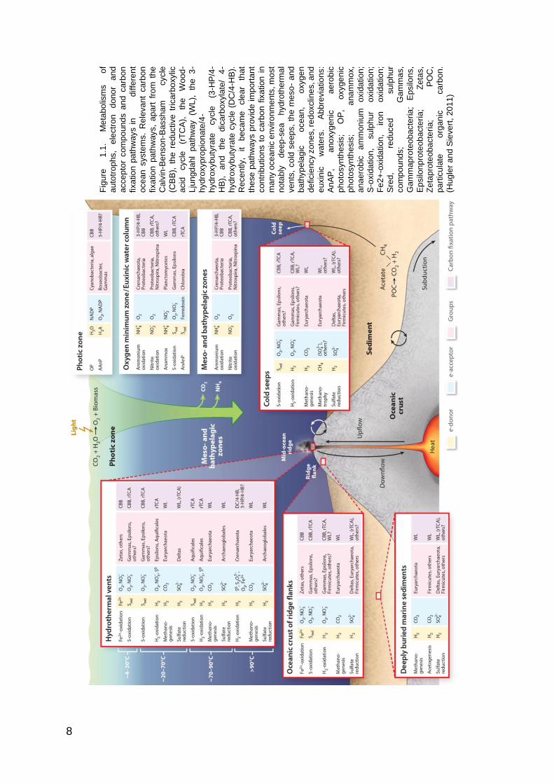
loaded in Thermal Cycler (ThermoFisher SCIENTIFIC): bacterial DNA was

amplified for 30 cycles (1 min of denaturation at 95°C, 1.5 min of annealing at

44°C, and 3 min of elongation at 72°C); archaeal DNA was amplified for 30 cycles

(1 min of denaturation at 95°C, 1 min of annealing at 55°C, and 2 min of

elongation at 72°C). The electrophoresis was performed on agarose gel (1%); in

order to control the reliability of PCR, positive and negative controls were used.

The gel was visualized under ultraviolet light after ethidium bromide bath. In

Figure 3.3, it is shown as the better results were obtained with FastDNATM SPIN

Kit for Soil.

FastDNATM SPIN Kit for Soil was selected to extract DNA from all the samples

reported in the Table S1. The FastDNA extraction is not a chloroform phenol

method; briefly the procedure followed these steps: i) the mechanical cell lysis is

carried out by a mixture of ceramic and silica particles; ii) the addition of reagents

permits to protect and solubilize nucleic acid upon cell lysis, minimize RNA

contaminations, enhance the protein precipitation; iii) the addition of a DNA

binding reagent allows the DNA holding; iv) the passage of DNA through a filter

permits the holding of DNA at the filter (this passage has to be repeated 3-4

times); v) the DNA is eluted in pure PCR water and stored at -20°C. After every

DNA extraction, DNA yield was measured.

The DNA concentrations of subsurface samples were lower than the surface

sediment (Table S1), thus the subsurface DNA was precipitated and suspended

in appropriate volume to have comparable concentration with surficial DNA

(precipitation procedure is described above). Furthermore, in order to have

comparable amount of DNA, I performed 2 extractions on surface samples and 4

21

extractions on subsurface samples. The DNA extracted from layers 0-1 cm and

1-5 cm was combined. A total of 2 g of sediment per samples were extracted from

both surface and subsurface layers.

To verify that the extracted DNA was amplifiable, I performed PCR on all the

extracted DNA samples (with the same procedure described above). I had some

problems to amplify archaeal DNA, which were resolved changing annealing

temperature, PCR reaction mixture and using a pair of primers that amplify a

shorter fragment (958R [5’-CCGGCGTTGANTCCAATT-3‘] and 20F).

In the Table 3.3, the selected and shipped samples are shown; the Figure 3.4

shows PCR products on electrophoresis gel of these final samples.

Figure 3.3. Electrophoretic run in agarose gel (1%) for PCR products (amplified 16S segments) of DNA extracted with different kits; a)archaeal 16S; b)bacterial 16S. Highlighted in red are the DNA samples extracted with FastDNATM SPIN Kit for Soil.

22

Figure 3.4. Results of PCR for testing the 16S amplification of DNA for sequencing. a) bacterial samples; b) archaeal samples. La, low DNA Mass Ladder; PCb, Positive Bacterial Control; NCb, Negative bacterial Conrol; PCa, Positive Archaeal Control; NCa, Negative archaeal Control. In yellow are the 0-10 cm sediments; in orange the 110 cm sediments; in blue the 410 cm sediments.

Table 3.3. Table that reports DNA concentrations, volume, amount and 260/280 and 260/230 ratios of DNA samples that were shipped for the amplification.

Station Depth bsf DNA Concentration Volume Amount of DNA 260/280 260/230

cm ng/ul ul ng

A0 0-5 19.2 10 192.2 1.91 0.03

A1 0-5 21.0 10 209.9 1.85 0.04

A2 0-5 21.8 10 217.6 1.94 0.04

A2m 0-5 17.2 10 171.7 2,00 0.03

A3 0-5 8.0 13 103.9 2.49 0.01

A3m 0-5 13.2 10 132.0 1.9 0.02

A1 110 16.2 10 162.2 1.49 1,00

A2 110 17.6 10 176.1 1.62 0.67

A3 110 18.5 10 185.5 1.62 1.37

A1 410 17.8 10 178.8 1.58 0.5

A2 410 17.0 10 169.9 1.53 0.61

A3 410 18.3 10 183.3 1.61 0.7

23

3.4 DNA Sequencing

The extracted DNA was shipped to CeBiTec laboratory (Centrum für

Biotechnologie, Universität Bielefeld) and was sequenced with the Illumina MiSeq

platform. For 16S amplicon library preparation we used bacterial primers 341F

(5´-CCTACGGGNGGCWGCAG-3´) and 785R (5´-GACTACHVGGGTATC

TAATCC-3´) and archaeal primers Arch349F (5´-GYGCASCAGKCGMGAAW-3´)

and Arch915R (5´-GTGCTCCCCCGCCAATTCCT-3´), which amplified 16S

region V3-V4 for Bacteria (length fragment 420 bp) and V4-V6 for Archaea (length

fragment 510 bp).

The amplicon library was sequenced with the MiSeq v3 chemistry, in a 2x300

bases paired device. The Illumina sequencing mechanism is, briefly: i) short DNA

sequences (adaptors) are attached to the DNA fragments; ii) DNA segments are

denatured with sodium hydroxide, and made single stranded; iii) once prepared,

the DNA fragments are washed across the flowcell and the complementary DNA

binds to primers on the surface of the flowcell whereas the DNA that doesn’t

attach is washed away; iv) the DNA attached to the flowcell is replicated to form

clusters of DNA with the same sequence; these clusters have to be big enough

to emit a strong signal that will be detected by a camera; v) unlabelled nucleotide

bases and DNA polymerase are added to extend and join the strands of DNA

attached to the flowcell. This creates ‘bridges’ of double-stranded DNA between

the primers on the flowcell surface; the double-stranded DNA is then denatured

into single-stranded DNA using heat, leaving several million dense clusters of

identical DNA sequences; vi) primers and fluorescent labelled terminators,

nucleotide bases that stop DNA synthesis, are added to the flowcell; vii) the

primer attaches to the DNA being sequenced, vii) the DNA polymerase then binds

24

to the primer and adds the first fluorescently-labelled terminator to the new DNA

strand. Once a base has been added no more bases can be added to the strand

of DNA until the terminator base is cut from the DNA; ix) lasers are passed over

the flowcell to activate the fluorescent label on the nucleotide base; the

fluorescence is detected by a camera and recorded on a computer; each of the

terminator (different bases) emits in a different colour; x) the fluorescently-

labelled terminator group is then removed from the first base and the next

fluorescently-labelled terminator base can bind the DNA stand; this process

continues until millions of clusters have been sequenced.

The output of the this sequencing are millions of reverse and forward reads that

overlap for a variable number of base pairs, depending on the used primer; in our

samples the overlap is about 40-80% for bacteria and about 30% for archaea.

Thus the reverse and forward reads had to be merged before to analyze the

sequencing date, as well as cleaning and quality control was carried out. The

Table 3.4 reports the number of sequences before and after cleaning and

merging. First, I removed the primers from the reads with the command-line tool

cutadapt (Martin, 2011). Then I used the software TRIMMOMATIC (Bolger et al.,

2015) in order to remove the sequences that did not have a good quality; this

step has been performed before the reads merging for bacteria and after merging

for archaea. The difference in the procedure is due to the different length of the

segments (and consequently, the overlapped region between reverse and

forward reads). The quality of the sequencing is usually lower at 3’-region of the

reads (Bartram et al., 2011), so if there are long fragments, as I have for archaea,

it is better performed the trimmomatic step after the merging because these could

enhance the number of the holding reads. The merging step was performed with

25

the PEAR software (Zang et al. 2013). The operational taxonomic unit (OTU)

clustering has been made with SWARM (Mahè et al. 2014). OTUs were built with

a similarity threshold of 97%. I used this method because the clustering is low

influenced by clustering parameters and products robust OTUs. The taxonomic

classification is based on SILVA database (Quast et al., 2013). During this step,

sequences with less than 90% of similarity with SILVA sequences have been

removed; this removal was done in order to remove the presence of amplification

and sequencing artifacts, as chimera; the weakness of this approach is the high

probability to exclude unknown organisms.

3.5 Statistical analysis

All analyses were carried out in the R statistical environment (R Development

Core Team, 2009) with the packages vegan (Oksanen et al., 2010) and ggplot2

(Wickham, 2009), as well as with custom R scripts.

The bacterial and archaeal communities of surface and subsurface sediments

were analyzed separately. The number of singletons, doubletons and unique

OTUs was calculated separately for surface and subsurface. Singletons (SSO)

a

A0 A1 A2 A2m A3 A3m A1 A2 A3 A1 A2 A3

Reads* 87522 123394 59037 55752 39162 54320 169752 159425 92251 48417 115178 146723

Clipped reads* 83590 118163 56328 53224 37440 51852 162567 152438 88613 46317 110355 140707

Trimmed reads* 83558 118126 56312 53195 37431 51833 162498 152383 88574 46295 110324 140663

Assembled reads 82921 117610 56083 52985 37130 51583 161040 151510 88019 45941 109743 139931

b

A0 A1 A2 A2m A3 A3m A1 A2 A3 A1 A2 A3

Reads* 51982 57240 52121 59126 52415 96761 58347 63821 52467 59727 52298 50405

Clipped reads* 32171 39895 33848 38961 40481 71740 46766 44516 41141 49139 37144 38872

Assembled reads 27023 33308 28817 33633 30577 58977 27556 31290 30787 32840 28368 30339

Trimmed reads 3666 3464 3657 6502 10456 11691 2466 5104 3711 4833 2528 4901

0-5 110 410

0-5 110 410

Table 3.4. Table with number of reads after every steps of the quality cleaning. *these numbers represent only the reverse or forward reads, as these steps were performed before the reads merging.

26

are defined as the OTUs that are represented with one sequence in the entire

dataset; doubletons (DSO) are the OTUs that are presents with two sequences

in only one sample; and unique OTU (OTUunique) are OTUs that are present only

in one samples but with more than 2 sequences. With absolute percentage

(SSOabs, DSOabs and OTU unique abs) I refer to number of singletons, doubletons

and unique OTUs present in a sample relative to total number of OTUs of the

surface or subsurface dataset, whereas with relative percentage (SSOrel) I refer

to the contribution of singletons present in a certain sample to total number of

OTUs for that sample.

Inverse Simpson (InvS), Exponential Shannon (ExpS), and Chao1 were

calculated on a subsampled community to minimize the influence of errors due

to the DNA amplification and sequencing. Subsampling was performed randomly

taking in consideration the minor number of sequences (30826 for Bacteria and

2073 for Archaea). In order to assess if the subsampling invalidated Chao1,

ExpS, InvS indexes and the nOTU, Mantel tests were performed on Eucliden

matrixes calculated on those indexes values (calculated with and without

subsampling). Furthermore, to calculate if the community structure (CS) between

subsampled and not sampled dataset changed, Mantel test was performed on a

Bray-Curtis dissimilarity matrix.

To study the diversity between different samples, beta diversity was calculated

applying Jaccard index on OTUs presence/absence matrix. Thus the beta-

diversity is here a OTUs turnover, showing the number of OTUs shared amongst

samples.

The other analyses where performed on the dominant community, here defined

as the community without the presence of singletons. Non-metric

27

multidimensional scaling (nMDS) scatterplots have been performed with average

method at OTUs and every taxa levels in order to visualize the main clusters and

patterns of the dataset.

Similarity Percentages (SIMPER) analysis was performed on OTU dataset to

identify the main OTUs responsible of differences observed in nMDS plot.

As the SIMPER analysis tends to underlines the most abundant objects that are

responsible for the observed dissimilarity, an in-depth analysis of the dataset was

performed in order to detect all the interesting taxa. Particular importance was

given to those taxa that were exclusively, or mainly present in A3 or that showed

a decrease abundance from A3 to A0. In addition, in order to have results less

biased as possible, I inspected taxa that showed highest relative abundances in

A0.

Taxa analyses were carried out with BLAST software (Camacho et al., 2009) and

the construction of phylogenetic trees.

3.6 Phylogenetic Tree’s Construction

The phylogenetic trees were constructed with Arb software (Ludwig et al., 2004)

for those taxa that were highlighted by SIMPER or that showed important

changes in relative abundance between areas. The aim of my phylogenetic trees

was to see where the prokaryotes more phylogenetically related to my sequences

where isolated and if metabolic information were available. The latter is a critical

issue, since microbial community of deep sea ecosystems are barely studied and

really few organisms have already been cultured (Sogin et al., 2006) so metabolic

information were not present for the majority of taxa present in my dataset.

First, the sequences of the studied taxon were aligned with SINA aligner (Pruesse

et al., 2012); then they were added to the Silva tree with Parsimony method.

28

Closest reference sequences were selected and used to build a new tree with

Maximum Likelihood method with bootstrap statistical analysis (500 repetitions);

the used software was RAxML 8 (Stamatakis, 2014).

Once, constructed the tree backbone with the referenced sequences, my

sequences were added with Parsimony method, without any change in the tree

topology.

I applied this procedure because the Illumina 16S tag sequencing produces

sequences too short (<550 bp) to allow the construction of a solid backbone tree,

which, for this reason, was built using only 16S segments longer than 900 bp.

Furthermore, because the taxonomy of the family DHVEG-6 changed recently

(Eme and Doolittle, 2015), for this archaeal family I choose to build a second

phylogenetic tree. The procedure for the construction of this tree has been the

same but, as reference sequences, I selected only organisms previously cultured

(Castelle et al., 2005). This approach allowed to better inferring about potential

metabolism of OTUs belonging this taxon.

The phylogenetic trees were ultimate in the R statistical environment (R

Development Core Team, 2009) with the packages phyloseq (McMurdie and

Holmes, 2014), ade (Paradis et al., 2004), ggplot2 (Wickham, 2009), stringi

(Gagolewski and Tartanus, 2015) and plyr (Hadley, 2011).

29

4. Results

Since the rare biosphere (i.e. singletons) represented the large fraction of total

OTUs and the number of sequences recovered showed an high variability

between samples (Table 4.1; Table 4.2), thus subsampling of Illumina sequences

was performed in order to normalize the dataset and therefore to have a better

comparison of alpha-diversity between samples.

Mantel test, showing a high correlation between alpha-diversity indexes and

community composition calculated on the whole dataset and the subsampling

dataset (Table 4.3), highlighted that the bacterial and archaeal diversity and

community structure in the subsampling dataset reflected the patterns observed

for whole dataset. For this reason, differences in bacterial and archaeal

community composition were analysed on whole dataset. Furthermore the rare

biosphere (i.e. the singleton component) was not taken into account for analysis

of differences in community composition. Conversely, to be conservative, in the

following section I described the OTU richness (number of OUTs) for whole

dataset and diversity indices (i.e. Chao1, Exponential-Shannon and Inverse-

Simpson) for subsampled dataset. Instead sequence number (nSeq), single-

sequence OTU or singleton (SSO), double-sequence OUT or doubleton (DSO)

and unique OTU (OTUunique) were referred to whole dataset.

4.1 Bacterial Diversity

4.1.1 Comparison between surface and subsurface

The sequencing dataset showed a variable number of sequences amongst

different samples (Table 4.1). In general, the sequence number was higher in

subsurface samples than in surface samples.

30

Table 4.1. Description of bacterial number of sequences, richness, alpha-diversity and rare biosphere at each site. a) surface layers; b) subsurface layers. nSEQ, total number of sequences; nOTU, number of OTUs; SSO, number of singletons; SSOabs, percentage of singletons relative to total number of OTUs; SSOrel, percentage of singletons relative to number of OTUs of each sample; DSO, number of doubletons; DSOabs, percentage of doubletons relative the total number of OTUs; OTUunique, number of unique OTU; OTUunique abs: percentage of unique OTUs relative to total number of OTUs. InvS, Inverse Simpson index; ExpS, exponential Shannon index. Subsampling was performed using the minimum bacterial sequences value (30826).

a

A0 A1 A2 A2m A3 A3m Tot

nSEQ 80637 112328 53776 50510 30826 45910 373987

nOTU 27721 31079 18347 16378 9264 14610 98710

SSO 23146 23070 12324 10971 6047 10191

SSOabs (%) 23.45 23.37 12.49 11.11 6.13 10.32

SSOrel (%) 83.50 74.23 67.17 66.99 65.27 69.75

DSO 376 705 186 206 275 460

DSOabs (%) 0.38 0.71 0.19 0.21 0.28 0.47

OTUunique 330 356 74 82 304 517

OTUunique abs (%) 0.33 0.36 0.07 0.08 0.31 0.52

Subsampling

nOTU 12100 11343 11872 11120 9264 10715

Chao1 95973 50049 57113 53657 41439 51152

InvS 285.43 663.45 888.37 703.37 454.89 586.43

ExpS 2752.97 3325.77 3915.25 3174.53 2174.39 2880.82

b

110 cm 410 cm

A1 A2 A3 A1 A2 A3 Tot

nSEQ 145953 141502 78211 41852 104178 126448 638144

nOTU 24732 23900 13264 11710 19929 21861 104839

SSO 21545 19504 10178 9163 16771 18137

SSOabs (%) 20.55 18.60 9.71 8.74 16.00 17.30

SSOrel (%) 87.11 81.61 76.73 78.25 84.15 82.97

DSO 291 410 230 123 202 387

DSOabs (%) 0.28 0.39 0.22 0.12 0.19 0.37

OTUunique 971 609 208 98 241 344

OTUunique abs (%) 0.93 0.58 0.20 0.09 0.23 0.33

Subsampling

nOTU 6724 6982 6257 9027 7082 6761

Chao1 42112 34914 34929 74467 50125 41660

InvS 92.63 64.61 55.25 113.34 38.02 47.26

ExpS 653.12 610.01 459.22 1058.43 517.80 478.38

0-5 cm

31

Table 4.2. Description of archaeal number of sequences, richness, alpha-diversity and rare biosphere at each site. a) surface layers; b) subsurface layers. nSEQ, total number of sequences; nOTU, number of OTUs; SSO, number of singletons; SSOabs, percentage of singletons relative to total number of OTUs; SSOrel, percentage of singletons relative to number of OTUs of each sample; DSO, number of doubletons; DSOabs, percentage of doubletons relative the total number of OTUs; OTUunique, number of unique OTU; OTUunique abs: percentage of unique OTUs relative to total number of OTUs. InvS, Inverse Simpson index; ExpS, exponential Shannon index. Subsampling was performed using the minimum bacterial sequences value (2073).

a

A0 A1 A2 A2m A3 A3m Tot

nSEQ 3433 3239 3442 6348 6936 9036 32434

nOTU 1704 1610 1699 2962 3694 4349 15463

SSO 1629 1502 1598 2859 3352 4044

SSOabs (%) 10.53 9.71 10.33 18.49 21.68 26.15

SSOrel (%) 95.60 93.29 94.06 96.52 90.74 92.99

DSO 4 2 0 1 47 39

DSOabs (%) 0.03 0.01 0.00 0.01 0.30 0.25

OTUunique 8 1 1 0 78 26

OTUunique abs (%) 0.05 0.01 0.01 0.00 0.50 0.17

Subsampling

nOTU 806 814 811 781 971 844

Chao1 36049 21475 19506 21941 8827 13316

InvS 65.38 56.15 45.07 43.63 111.58 32.11

ExpS 261.60 271.62 248.24 226.02 511.97 243.18

b

110 cm 410 cm

A1 A2 A3 A1 A2 A3 Tot

nSEQ 1565 3257 2746 3345 2073 4115 17101

nOTU 1058 1716 1646 1802 1133 1715 8724

SSO 986 1617 1556 1677 1053 1608

SSOabs (%) 11.30 18.54 17.84 19.22 12.07 18.43

SSOrel (%) 93.19 94.23 94.53 93.06 92.94 93.76

DSO 4 9 5 14 1 9

DSOabs (%) 0.05 0.10 0.06 0.16 0.01 0.10

OTUunique 3 14 5 9 1 8

OTUunique abs (%) 0.03 0.16 0.06 0.10 0.01 0.09

Subsampling

nOTU 1058 857 964 885 865 691

Chao1 30676 20666 27118 20308 32725 14960

InvS 141.13 54.00 59.03 64.56 43.46 23.53

ExpS 540.37 282.16 363.67 347.93 270.97 142.59

0-5 cm

32

The lowest number of sequences was found in the superficial sample A3 (30826

sequences) and the highest value was shown in the sample A1 (145953

sequences), collected at 410 cm bsf. The number of OTUs was also variable

between samples, with maximum value at the surface sample A1 (31079 OTUs)

and the minimum value at the surface sample A3 (9264 OTUs). The singleton

percentages per sample (SSOrel) were higher in subsurface, ranged between

76% and 87%, than in surface samples, ranged between 65% and 83%. Lowest

Chao1 was found at 110 cm in all areas (ranged between 34914 and 42112), and

the highest values were described for deeper subsurface layer in A1 (74467);

superficial samples ranged between 41439 and 57113. Inverse-Simpson (InvS)

and Exponential-Shannon (ExpS) indexes are higher in superficial samples (455-

888 and 2174-3915 respectively) than subsurface ones (38-113 and 459-1058).

4.1.2 Comparison between areas: surface

The maximum number of sequences and OTUs was found in A1 (112328 and

31079, respectively), whereas the lower values were observed in A3 (30826 and

9264, respectively). The number and relative abundance of singletons decreased

from A0 (23146 and 23%, respectively) to A3 (6047-10191 and 6-10%,

respectively). The expected richness (Chao1) was higher in A0 than SWIR areas,

Table 4.3. Mantel test performed on bacterial and archaea entire datasets and subsampled dataset. Mantel test on CS (Community Structure) has been performed on Euclidean distances matrix calculated on Bray-Curtis dissimilarity matrix; whereas, Mantel tests on Chao1 index, ExpS (Exponential Shannon) index, InvS (InverseSimpson) index and nOTU (number of OTUs) have been performed on Euclidean distance matrixes.

Test r p r p

CS 0.96 0.001 0.96 0.001

Chao1 0.96 0.001 0.98 0.001

ExpS 0.82 0.0005 0.95 0.001

InvS 0.86 0.001 0.67 0.014

nOTU 0.99 0.001 1.00 0.001

Bacteria Archaea

33

with lower richness in A3. InvS and ExpS indexes showed the lowest value in A0

and A3, and the highest in A2 (Table 4.1a).

4.1.3 Comparison between areas: subsurface

At 110 cm bsf we observed a decrease of the number of sequences and OTUs

from area 1 to area 3, whereas an opposite trend was found for samples at 410

cm bsf. The SSOabs was highest at A1 for layer 110 cm (20%) and lowest at A1

for layer 410 cm (8%). Chao1, InvS and ExpS were higher in A1 than A2 and A3,

in A1 these indices were higher at 410 cm than at 110 cm (Table 4.1b).

4.2 Bacterial Community Composition

The nMDS, performed on OTUs Bray-Curtis similarity matrix, showed two main

clusters composed by surface and subsurface samples (Figure 4.1); samples

inside these 2 groups had a dissimilarity values under the threshold of 90%.

Considering a threshold of 80%, the two superficial A3 samples established a

different cluster from the other surface samples; the same happens for the

subsurface samples A1. With a dissimilarity threshold of 50% other clusters are

formed: two superficial samples, A1 and control area, clustered separately;

subsurface samples of Area 1 clustered separately from each other (Figure S1).

nMDS performed at taxonomic levels (phylum, class, order, family and genus)

showed similar clusters (data not shown). Analysing beta-diversity along the

vertical profiles, the highest shared OTUs was between the two subsurface

layers, and the value ranged between 15% and 39%. Values between surface

and subsurface layers ranged between 0.4-6.5% (110 cm) and between 1.0-4.5%

(410 cm). At A3, the number of shared OTUs along vertical profile was highest

(6.5%, 39% and 4-4.5%, Figure 4.2c). Analysing horizontal surface profiles, the

lowest beta-diversity value was observed amongst A3 other areas (5-14%).

34

Instead, in the subsurface layers the shared OTUs were higher between A2 and

A3 (20%) than between A2 and A1 (13-18%; figure 4.2a).

4.2.1 Subsurface

The Figure 4.3 and Figure 4.4 show the relative abundance of the 10 most

abundant families and classes per samples, respectively, and their patterns in

areas investigated. At class level the differences between surface and subsurface

community’s composition were mainly driven by dominance of Dehalococcoida,

Candidate division OP8 and Candidate division JS1 in subsurface samples,

whereas Gammaproteobacteria, Deltaproteobacteria, Alphaproteobacteria,

Flavobacteria and Acidimicrobia were mostly present in superficial samples.

The Candidate division JS1 increased from A1 to A3 in both layers, conversely

Dehalococcoida and Candidate division OP8 did not show any consistent

patterns between stations and layers. Interesting 9 OTUs belonging to JS1 and

16 OTUs belonging OP8 explained 25%, 25% and 27% of differences between

Figure 4.1 Multi-Dimensional Scaling (nMDS) plot performed on bacterial community with average method. The broken line indicates a dissimilarity threshold of 80%.

35

Figure 4.2. Diagram of beta-diversity amongst different stations and layers. Beta-diversity has been calculated applying dissimilarity Jaccard index on OTUs presence/absence matrix. a) bacterial beta-diversity along vertical profiles; b) archaeal beta-diversity along vertical profiles; c) bacterial beta-diversity along horizontal profiles; d) archaeal beta-diversity along horizontal profiles. Values in the brackets refer to A2m and A3m stations.

36

Figure 4.4. Plot representing the 10 most relative abundant bacterial classes in each sample.

Figure 4.3. Plot representing the 10 most relative abundant bacterial families in each sample.

37

A3 and A1, between A2 and A1, and between A3 and A2, respectively (SIMPER;

Table S2). Phylogenetic trees of JS1 and OP8 candidate division showed that

these OTUs were phylogenetic related to bacterial clones found mainly in seeps,

volcanoes and other subsurface ridges (Figure 4.5; Figure 4.6). The OTU55 and

OTU105, belonging to the class Dehalococcoidia and explaining 0.8% of the

differences between A3 and other areas, showed a higher relative abundance at

A3 (2.4% and 1%, respectively) than at A2 and A1 (0.2% and 0.1%, respectively).

However the BLAST alignment showed that only OTU105 was close related to

Bacteria isolated from chemosynthetic environments (seep and mud volcano).

Four OTUs (OTU77, 17OTU, 40OTU and 146OTU), belonging to Candidate

Division KB1, had a relative abundance of 0.6%, 3.3% and 8.5%, respectively in

A1, A2 and A3, and in phylogenetic tree they were clustered close to bacteria

isolated from methane seeps (Figure 4.7).

4.2.2 Surface

The SIMPER highlighted that 25% of differences between surface community

structure at A3 and those at other areas (A0, A1 and A2) were explained by 47

OTUs, 77 OTUs, and 88 OTUs, respectively, belonging to 49 different bacterial

taxa (Table S3). Only for those OTUs whose relative abundance was higher at

A3 than at A0, A1 and A2 the phylogenetic trees were constructed. The OTUs

belonging to SEEP-SRB1 were present only in SWIR areas, and they were close

related to bacteria isolated from deep-sea seeps, volcano and ridge habitats

(Figure 4.8). In particular the OTU129 had a relative abundance of 0.2% and

1.8% at A3 and A3m, respectively, and explained 0.6-0.7% of differences in

nMDS plots between A3 and other areas. The bacterial family JTB255 showed

lowest relative abundance in A3 (Figure 4.3), however the relative abundance of

38

OUT187, belonging to not classified genus of JTB255, was higher at A3 (0.9-

1.3%) than at A1 and A2, whereas it was not present A0, and it explained 0.7%

of differences in bacterial community structure. The phylogenetic tree clustered

this OTU close to bacteria isolated from ridge and hydrothermal systems (data

not shown). The OTU224 belonging to bacterial class VC2.1 Bac22 showed a

higher relative abundance in A3m (1.1%) than A3 (0.03%) and it was nearly

absent in other areas. The phylogenetic tree showed this OTU clustered with an

endosymbiont chemolithoautotrophic bacteria (Figure 4.9). The OTU170 and

OTU101 belonging to Family SAR406 clade (Marine Group A) were dominant

OTUs at A3 (1.6-1.7%, respectively) and explained 1.5-1.7% of differences

between bacterial community at A3 and those at A0, A1 and A2. Closer related

bacteria were found in marine sulfide deposit and ridge methane seeps (Figure

4.10). Furthermore, the OTU6369 and OTU6594 were found only in A3 surface

samples (0.06% and 0.04% in A3 and A3m; respectively), and they were

phylogenetically close to chemolithoautotroph bacterial clones. The differences

in surficial bacterial community structure were also driven for 0.9-1% by OTU150

and OTU173 (family Anaerolineaceae), whom were present only at A3 (0.4-1%)

and related bacteria were found in deep-sea methane and oil rich environments,

and ridge fluids (data not shown). The Family Desulfarculaceae was found only

in A3, representing 5.3% of bacterial community. In particular the OTU498 and

OTU408, contributing to explain 0.3-0.4%, respectively, of SIMPER analysis,

were clustered close to bacteria isolated from hydrothermal, mud volcano and oil

polluted marine sediments (data not shown). The relative abundance of OTU402

and OTU794, belonging to phylum Candidate Division OP8, was 0.3% and 1.2%

at A3 and A3m, respectively, and they were not found in other areas. They

39

explained 0.3-0.5% of difference in surficial community structure and were

clustered close to bacteria isolated from deep-sea sediments and anaerobic

methanotrophs isolated from mud-volcano (Figure 4.6). The OUT507, OTU599,

OTU698 represented 1.3% of bacterial community at A3m, less than 0.1% in

other SWIR areas, and they were not present in reference area. They belonged

to family WCHB1-69, and they explained 0.3% of differences between areas.

OTU507 and OTU698 clustered close to bacterial clones found in deep sea

hydrothermal vent, terrestrial sulphide spring and hypersaline microbial mat.

OTU599 clustered close to coral endosymbiont clones (data not shown). The

OTUs belonging to subsurface phylum Candidate division JS1 (OTU48, OTU131

and OTU4) were only present in A3, with a relative abundance of 0.9-1.1%, and

explained 0.7% of differences between bacterial communities. OTU131 and

OTU48 clustered close to mud volcano and anoxic fjord bacterial clones; whereas

OTU4 close to subsurface drilling sediment clones (Figure 4.5). Sulfurovum and

Sulfurimonas (family Helicobacteraceae) were not selected by SIMPER, however

they were exclusively present in A3, with highest relative abundance at A3m

(0.9%). These genera include chemolithotrophic bacteria isolated from marine

hydrothermal vents and cold seep systems (Figure 4.11).

The genus Spirochaeta showed an abundance of 1.3-1.5% in A3, whereas it is

lower in the other areas. The phylogenetic tree showed that the OTUs, here found

belonging to this genus, were related to systems of hydrothermal vents and

methane seeps (data not shown). The genus Acidiferribacter showed a relative

abundance of 0.6% and 0.2% in A3m and A3, respectively, and it was absent in

A0; the analysis performed on BLAST platform highlighted its phylogenetic affinity

to chemosynthetic organisms.

40

Furthermore, a crosscheck was carried out on OTUs that were highlighted by the

SIMPER and that showed higher relative abundance in A0. The analysed taxa

S085, Pseudomonas, Rubritalea, Candidate Division OM1 were found correlated

with bacterial clones previously isolated from deep sea sediment.

4.3 Archaeal Diversity

4.3.1 Comparison between surface and subsurface

Superficial samples showed a higher number of sequences than subsurface

samples, ranging between 3239-9036 and 1565-4115, respectively (Table 4.2).

Number of OTUs showed a similar trend, with 1610-4349 OTUs in surficial

samples and 1058-1802 in subsurface samples. The SSOrel was 91-96% and 93-

95% for surficial and subsurface samples, respectively. The percentage of

OTUunique was lower than 0.2% in all samples. Chao1 ranged between 8827 and

36049 in surface samples, and between 14960 and 32725 subseafloor layers.

InvS showed values between 32 and 111 in surface layer and between 23 and

141 in subsurface layers. In surface samples, ExpS had a minimum value of 226

and a maximum value of 512, and it ranged between 143 and 540 in subsurface

samples.

4.3.2 Comparison between areas: surface

The highest number of sequences and OTUs was observed in A3 (6936-9036

and 3694-4349, respectively) and in the sample A2m (6348 and 2962,

respectively); in the other samples these values were less than 3500 sequences

and 1800 OTUs. Highest SSOabs was observed in A3 and A3m (22% and 25%;

respectively); in other areas, this value ranged between 10% (A0, A1 and A2)

and 18% (A2m). Highest Chao1 value was calculated for A0 (36050), inside the

SWIR the estimated richness decreased from A1 to A3 (21475-8827). InvS and

41

ExpS decreased from A0 to A3m (65.4-32.1 and 162-243, respectively), however

highest values were observed for A3 (111.6 and 512, respectively; Table 4.2a).

4.3.3 Comparison between areas: subsurface

In A1 and A3 the number of sequences and OTUs increased from 110 cm to 410

cm bsf, whereas an opposite trend was observed for A2. SSOabs didn’t show any

pattern between areas and layers; this value ranged between 11% and 19%.

Chao1 didn´t show any consistent trend between areas and layers. InvS and

ExpS were higher at A1 than at A2 and A3, and they decreased from 110 cm to

410 cm (bsf) in all areas (Table 4.2b).

4.4 Archaeal Community Composition

The NMDS plot showed that the A0 clustered separately from SWIR areas with

a dissimilarity value of 70% (Figure 4.12). Considering a dissimilarity threshold of

60%, the superficial sample A3 clustered apart from the other samples. Whereas

with the 40% of dissimilarity, four other clusters formed: A2 subsurface layers and

A1 110 cm layer; A1 410 cm layer; both A3 subsurface layers and A3m surficial

layer; A1 and A2 surficial layers (Figure S2).

Beta-diversity along vertical profile of A1 and A3, the surficial layer shared a major

number of OUTs with deeper layer (410 cm) than with 110 cm. In A2 the number

of OUTs shared between surficial layer and subseafloor layers decreased with

sediment depth. In A2 and A3 the shared OTUs between subsurface layers were

higher than those shared between surface layer and subsurface layers.

42

Conversely, in A1 the shared OTUs between subsurface layers were lower than

those shared by surface and 410 cm layers (Figure 4.2d).

The analysis of surficial beta-diversity showed the same pattern observed for

bacterial beta-diversity. I observed a lower number of shared OTUs between A2

and A3 than between A2 and A1, and a higher number of shared OTUs between

A1 and A0 than between A1 and A3, with lowest OTUs shared between A3 and

A0. In the 110 cm layer the beta-diversity decreased with distance between

areas, conversely in 410 cm layer the number of shared OTUs between A2 and

A3 was higher than between A2 and A1 (Figure 4.2b).

4.4.1 Surface and subsurface

At A0, the archaeal community was dominated by unclassified archaea belonging

to Marine Group I and by Candidatus Nitrosopumilus (Figure 4.13). The latter

dominated also in surficial and subsurface samples at SWIR areas, with

exception for superficial station A3, where the dominant archaeal family was

Figure 4.12. Multi-Dimensional Scaling (nMDS) plot performed on archaeal community with average method. The broken line indicates a dissimilarity threshold of 70%.

43

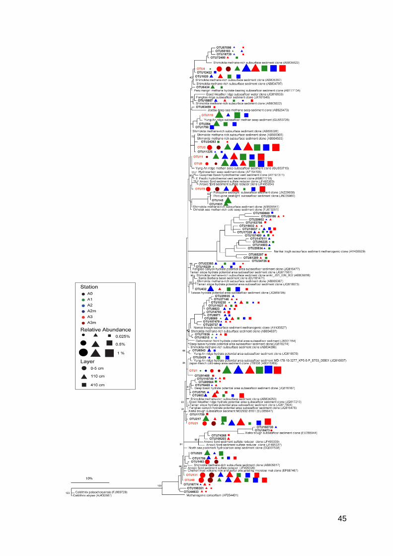
Deep Sea Hydrothermal Vent Gp 6 (DHVEG-6; 53%). In subsurface layers other

two important taxa were Marine Benthic Group D and Deep Sea Hydrothermal

Vent Gp 1 (MBGD and DHVEG-1) and Group C3. The highest relative abundance

of MBGD and DHVEG-1 was found in A1 (21% in the 110 cm layer and 16% in

410 cm layer); it was about 7% in A2 and 5% in A3. The relative abundance of

C3 showed higher values in the deepest layer, here the value ranged between

9% and 12% in contrast with the 110 cm layer where the values ranged between

5% and 8%. Interesting phylogenetic tree showed that the majority of OTUs,

belonging to DHVEG-6, clustered close to archaea isolated from hydrothermal

and seep environments (Figure 4.14). Likewise, OTUs belonging to MBGD and

DHVEG-1 were related to archaea identified in chemosynthetic environments

(data not shown). The family Diapherotrites was found exclusively in surficial

sediments of A3, and in particular the OTU47, representing 2.7% of archaeal

community in the superficial sample of A3, was close to hydrothermal archaea in

phylogenetic tree (data not shown). Five OTUs belonging to Marine Hydrothermal

Vent Group (MHVG) were also found only at A3 (1.2%) and they were related to

archaea described for chemosynthetic and methanogenic environments.

Figure 4.13. Plot representing the most abundant archaeal families in the dataset. *genus level

44

The phylogenetic tree of Marine Group I showed lack of differential OTUs

clustering amongst investigated areas, with related archaea isolated both from

deep-sea and hydrothermal systems (data not shown). Furthermore, I analysed

OTUs belonging to the genus Candidatus Nitrosopumilus on the BLAST platform

and, of particular concern is the OTU1 that was dominant at A3 (with a relative

abundance of 27% in A3m), showed a decreasing trend from A2 to A0 (2%) and

resulted phylogenetically close to methane-seep archaeal clones.

Figure 4.5. Phylogenetic tree of the phylum Candidate Division JS1. The tree backbone was constructed, including only the reference sequences, with Maximum Likelihood Method and 500 bootstraps were performed; then SWIR JS1 sequences were added with Parsimony Method. SWIR JS1 sequences are bolded. Red writings indicate highlighted OTUs by the SIMPER. (next page)

45

46

47

Figure 4.6. Phylogenetic tree of the phylum Candidate Division OP8. The tree backbone was constructed, including only the reference sequences, with Maximum Likelihood Method and 500 bootstraps were performed; then SWIR OP8 sequences were added with Parsimony Method. SWIR OP8 sequences are bolded. Red writings indicate highlighted OTUs by the SIMPER. (previous page)

Figure 4.7. Phylogenetic tree of the phylum Candidate Division KB1. The tree backbone was constructed, including only the reference sequences, with Maximum Likelihood Method and 500 bootstraps were performed; then SWIR KB1 sequences were added with Parsimony Method. SWIR KB1 sequences are bolded. Red writings indicate highlighted OTUs by the SIMPER.

48

Figure 4.8. Phylogenetic tree of the genus SEEP-srb1. The tree backbone was constructed, including only the reference sequences, with Maximum Likelihood Method and 500 bootstraps were performed; then SWIR SEEP-srb1 sequences were added with Parsimony Method. SWIR SEEP-srb1 sequences are bolded. Red writings indicate highlighted OTUs by the SIMPER.

49

Figure 4.9. Phylogenetic tree of the order VC2.1 Bac22. The tree backbone was constructed, including only the reference sequences, with Maximum Likelihood Method and 500 bootstraps were performed; then SWIR VC2.1 Bac22 sequences were added with Parsimony Method. SWIR VC2.1 Bac22 sequences are bolded. Red writings indicate highlighted OTUs by the SIMPER.

Figure 4.10. Phylogenetic tree of the family Sar406. The tree backbone was constructed, including only the reference sequences, with Maximum Likelihood Method and 500 bootstraps were performed; then SWIR Sar406 sequences were added with Parsimony Method. SWIR Sar406 sequences are bolded. Red writings indicate highlighted OTUs by the SIMPER. (next page)

50

51

Figure 4.11. Phylogenetic tree of the family Helicobacteraceae. The tree backbone was constructed, including only the reference sequences, with Maximum Likelihood Method and 500 bootstraps were performed; then SWIR Helicobacteraceae sequences were added with Parsimony Method. SWIR Helicobacteraceae sequences are bolded.

Figure 4.14. Phylogenetic tree of the archaeal family DHVEG-6. The tree backbone was constructed, including only the reference sequences, with Maximum Likelihood Method and 500 bootstraps were performed; then SWIR DHVEG-6 sequences were added with Parsimony Method. SWIR DHVEG-6 sequences are bolded. (next page)

52

53

5. Discussion

The segment 10°-16°E of South West Indian Ridge (SWIR), with a spreading

speed of only 8 mm/year, is the slowest segment of any other spreading ridge

(Dick et al. 2003). Despite the low spreading rate and the reduced magma input,

Bach et al. (2002) measured temperature and turbidity anomalies in bottom water

of this SWIR section, suggesting the presence of hydrothermal emissions. To

confirm the presence of hydrothermal circulation, in 2013 the expedition

ANTXXIX/8 was carried out employing seismology, geology, microbiology, heat

flow analyses and others. The presence of hydrothermal plume in bottom water

was not confirmed and it has not been observed water/gas emissions at seafloor.

However, anomalies in heat flow, typically a signature of magma upwelling, and

pore water biogeochemistry and also the recovery of organisms related to fauna

vents suggested the existence of some type of hydrothermal circulation at SWIR.

The results of this intensive survey allowed to identify three areas with different

properties: Area 1 (A1) with higher heat flux below the seafloor; Area 2 (A2) where

in 2002 it was hypothesized the presence of hydrothermal emissions (Bach et al.,

2002), but not confirmed by expedition ANTXXIX/8; Area 3 (A3) with anomalies

of methane, ammonium, sulphide and dissolved inorganic carbon (DIC) in pore

water sediment profiles, and recovery of fauna vents (i.e. Vesicomyid clam and

tube worm Pogonophora).

The hypothesis of my thesis is that the presence of hydrothermal fluxes, changing

the sediment geochemistry, is responsible of benthic microbial community

modification. In particular, the biogeochemistry observed in this A3 could support

chemolithoautotrophic prokaryotes and specific microbial consortia. To test this

hypothesis I analyzed sediment samples collected in three SWIR’s areas (A1, A2

54

and A3) and in a reference area (A0), located outside and south to the ridge. In

order to assess differences in benthic prokaryotic assemblage between areas,

Illumina 16S gene tag sequencing was applied to describe bacterial and archaeal

diversity and community structure. Statistical tools were used to highlight

differences amongst areas and identify prokaryotic taxa responsible for these

differences. Furthermore, with the construction of phylogeny trees, I investigated

relationship between the OTUs identified in this study and Bacteria and Archaea

found in deep-sea chemosynthetic environments (e.g. hydrothermal vents, cold

seeps, hydrate-bearing sediments, mud volcanos).

The comparison of bacterial and archaeal community structure showed that A3

held a different prokaryotic community compared to other SWIR’s areas (mostly

for Bacteria) and reference area, both Bacteria and Archaea (Figure 4.1; Figure

4.12). In particular it is relevant that Bacteria, representing the dominant

prokaryotic domain in all stations investigated (relative abundance higher than

70%; data not shown), showed a community composition very different to those

observed in other areas (up to 70% of dissimilarity). The presence of specific

bacterial and archaeal communities in A3 was also supported by analysis of beta-

diversity (i.e. OTUs turnover). The A3 shared less OTUs with A2 than those

shared between A2 and A1, despite A2 was closer to A3 than A1 (Figure 4.2).

Even the reference area, which was about equally distant from all the SWIR

areas, shared more OTUs with A1 and A2 than with A3. Thus prokaryotic taxa

turnover at A3 did not show a typical distant-decay relationship, as expected for

deep-sea surface sediments (Zinger et al., 2014). Indeed under homogenous

environmental setting and not isolate ecosystems (e.g. without physical or

biogeochemical barriers), the similarity in taxonomic composition of biological

55

assemblages decreases with increasing of geographic distances (Nekola and

White, 1999). Conversely taxa turnover at A3 is similar to those describe for

microbial communities at hydrothermal/seep environments, where, due to the

presence of biogeochemical barriers, the microbial assemblages are isolated

from other environments, sharing with them lowest number of taxa (Zinger et al.,

2011; Ruff et al., 2014). Also the alfa-diversity suggests the presence of

hydrothermal related bacterial and archaeal communities at A3. Both bacterial

and archaeal OTUs estimated richness were lower at A3 than at other areas. The

decrease of diversity and increase of endemism is expected in presence of

hydrothermal/seep fluxes, which, leading a supply of chemical energy sources

and a highly reduced environment, favours the development of a microbial

community dominated by specialised taxa (Leibold et al., 2004; Ruff et al, 2014).

The higher bacterial diversity and the increase of rare biosphere observed in

other SWIR and reference areas align with what previously findings for the deep-

sea environment (Sogin et al., 2006).

The bacterial and archaeal communities in subsurface layers investigated, 110

cm and 410 cm below seafloor (bsf), were weakly area specific (Figure 4.3; Figure

4.4; Figure 4.13) and they did not show substantial differences in alpha-diversity

(Table 4.1; Table 4.2). A reason could be that, in general, the subsurface

sedimentary compartment is more homogenous than the surface habitat (Takai

et al., 2004). Unfortunately the lack of reference samples for these layers makes

not possible to assess if the similarity between SWIR areas may be due or not to

a hydrothermal circulation effect on subsurface environment along all rift valley.

Analysing bacterial beta-diversity along vertical sediments profiles, I observed

that at A3 the subsurface layers shared a higher numbers of OTUs with surficial

56

layer compared to what saw at A2 and A3. Furthermore at A3 the surficial and

subsurface bacterial communities were more similar to each other than at A2 and

A1 (Figure 4.2c). Since the differentiation of microbial community with sediment

depth is mainly driven by sediment burial and aging (Durbin and Teske, 2011),

the higher beta-diversity and similarity of bacterial communities observed at A3

can be due to the presence of hydrothermal circulation, which promotes

exchanges between surface and subsurface environments.

Some of dominant bacterial and archaeal classes identified in area 3 are typically

described also for deep-sea hydrothermal and seep systems, and these are

Deltaproteobacteria and JS1 for Bacteria, and Halobacteria and Thermoplasmata

for Archaea (Anderson et al., 2015; Ruff et al., 2015; Webster et al., 2004;

Harrison et al., 2009). Conversely the reference area is dominated by deep-sea

benthic taxa, such as Gammaproteobacteria, Alphaproteobacteria,

Acidomicrobiia and Planctomycetacia (Figure 4.3). Interesting A0 showed a

bacterial community composition similar to that described by Ruff and colleagues

(2014) for station located in Antarctic Polar Front, at northeast of the SWIR

(52,011 °S; 10,011 °E). This station was characterized by thick diatom ooze,

which was also observed in SWIR stations. The presence of this diatom ooze in

deep-sea sediments is typical for the Antarctic Polar Front, whereas it did not

occur south of SWIR, where the reference area (A0) was located, which sediment

is dominated by siliciclastic clay (Dutkiewicz et al. 2015). Despite the areas

outside the SWIR have different sedimentary properties (i.e. sediment

composition and porosity), bacterial communities were more similar than the

communities between the northern site and A3, even if, here, the sediment had

the same composition. For example, Rhodospirillaceae, Rhodobacteraceae,

57

Sh766B-TzT-29, Planctomycetaceae, Phycisphaeraceae and Acidobacteraceae

are taxa that in both the reference sites compose the majority of the bacterial

dominant community and they are barely represented in A3.

The highest bacterial sequences phylogenetically related to bacteria isolated in

hydrothermal and seep environments were found in Area 3, reaching 40-43% of

dominant community (defined here as those OTUs that are present with more

than one sequence in the whole dataset). Furthermore the percentage decreased

with the distance from A3, with lowest value at reference area (<5%; Figure 5.1).

The same trend was observed in archaea dominant community: in A3 the

community was constituted for 40-70% by sequences related to Archaea found

in deep-sea hydrothermal vents and seeps. In the reference area, only 2% of

archaeal sequences were associated with seep and hydrothermal isolated

(Figure 5.2). At studied areas, the potential chemolithoautotrophic organisms

constituted a minor part of the dominant bacterial and archaeal communities. In

fact, it represented about 6% of all the sequences; 4% of which was found in A3

(Figure 5.1). I decided not to include ammonia oxidizing organisms in this

estimate, like bacterial Nitrosomonas and archaeal Nitrosopumilus, since the

oxidation of ammonia is a process not related only to hydrothermalism, as the

ammonia is a product of organic matter degradation, and these taxa are

ubiquitous in marine sediments (Vannelli et al., 1990; Walker et al., 2010). In my

dataset the chemolithoautotrophic community was composed by bacteria

belonging to Epsilonproteobacteria, Acidoferribacterales, Sar406 and VC2.1

Bac22. The phylum Epsilonbacteria is usually dominant in hydrothermal systems

(Nakagawa et al., 2005). The found genera are Sulfurovum, Sulfurimonas and

Arcobacter, which are classified as sulphur oxidizers (Nunoura et al., 2012).

58

Figure 5.1. Histogram showing the relative abundance of bacterial sequences close related to hydrothermal –driven systems. The sequences close related to chemolithoautotrophic bacterial clones are in yellow.

Figure 5.2. Histogram showing the relative abundance of archaeal sequences close related to hydrothermal –driven systems.

59

Another potential sulphur oxidizers belonged to Acidoferribacterales (Hallberg,

2011), which was also identify in A3. Interesting, the higher sulphide

concentrations in A3 pore water than in other investigated areas supports the

presence of these chemolithotrophs.

Other two taxa that showed phylogenetic related with chemolithoautotrophic were

Sar406 and Vc2.1 Bac22 (Figure 4.9; Figure 4.10). Sar406 is particularly

abundant in oxygen depleted environments and supposed to have a sulfur-based

energy metabolism (i.e. dissimilatory sulphur oxidation; Wright et al., 2014),

whereas Va2.1bac22 has been found manly in hydrothermal plume (Meyer et

al.2013) and as endosymbiont of hydrothermal fauna (Alain et al. 2012).

The low contribution of chemolithotrophs is the main difference with prokaryotic

communities described so far for many deep-sea hydrothermal vents (Tyler et al.,

2003). However, the composition of hydrothermal fluids can be very different

(German and Seyfried, 2014) and therefore give rise to different communities of

chemolithotrophs (Boetius, 2005; Dick et al., 2013). The well investigated fast

and slow spreading ridges showed that vent-fluid compositions depend on

lithospheric substrate, with which hydrothermal fluids interact, and on origin of

heat (i.e. magmatism vs tectonism; German and Seyfried, 2014). At one extreme

there are the black-smokers in basal systems with a hydrothermal circulation

generated by magma upwelling and with acid (pH 3 to 5) and high temperature

(200°C to 400 °C) fluids enriched in CO2 and sulphide, which are inhabited mostly

by acidophilic, hyperthermophilic sulphite oxidizers (Boetius, 2005). At the other

extreme there are the white-smokers in ultramafic systems fuelled by tectonism

(i.e. serpentinization reactions), which, providing high fluxes of hydrogen and

methane at warm temperatures and high pH, sustains hydrogen and methane

60

oxidizing communities (Kelly et al., 2005; Kelly et al., 2007). The ultraslow

spreading ridges began to be explored only 15 years ago, and if little is known

about the origin of hydrothermal circulation, venting properties and fluids

compositions (Snow and Edmonds, 2007; German et al., 2010), the knowledge

of microbial diversity is practically absent (Peng et al. 2011). However one

important peculiarity of ultraslow speeding ridges is thin crust thickness (<1 km;

Dick et al., 2001). The lack of ocean crust allows to deep seawater to more easily

reach the mantle, which loss of heat can contribute and interplay with tectonic on

the formation and evolution of hydrothermal circulation even when magma supply

is limited. The presence of geochemical anomalies in axial region of SWIR, the

lack of abundant vent fauna and chemolithotrophs, here observed, could support

the presence of widespread low temperature diffuse fluid leakage generated by

loss of heat from the mantle.

Although the other chemosynthetic environment related taxa were not classified

like autotrophic prokaryotes, some of them are key taxa in support of my

hypothesis, since they are partners of consortia and/or mediate specific reaction

(e.g. hydrocarbon degradation) typically described for hydrothermal and seep

environments. SEEP-srb1 is a heterotrophic sulphate reducing (SR) organism

mainly found in seep systems. This taxon usually forms specific consortia with

ANME-2, a methanotrophic archaea, in hydrothermal and seep systems (Orcutt

et al., 2010; Orphan et al. 2010). To these consortia is attributable the anaerobic

oxidation of methane (AOM). ANME archaea oxidase methane and transfer the

obtained electron to SR bacteria through an unknown mechanism (Schreiber et

al. 2010); the electron is used by SR bacteria to reduce sulphate to sulphide.

Despite the methane anomalies found at A3 could support the presence of these

61

consortia, in the dataset, I didn’t find the archaeal partner (ANME-2) that usually

forms consortia with SEEP-sbr1. The lack of ANME-2 could be ascribed to

methodological problems like the non-specificity of the primers used (Ding et

al.,2015) or the DNA extraction procedure or the low amount of archaeal DNA.

Another problem could be the lack of knowledge about metabolism of

uncultivated archaea, indeed in my dataset several archaea taxa were found

mainly at A3 but for which metabolism is unknown (Takano et al., 2010).

In the dataset I found two other SR bacteria belonging to the phylum

Deltaproteobacteria: Desulfarculaceae and WCHB1-69. These bacterial families

are not exclusive of seep systems (Kuever, 2014; Okabe et al., 2003), however

the OTUs here found were phylogenetically close to seep bacterial clones. In the

work of McGlynn et al. (2015) consortia between ANME and organisms belonging

to the phylum Deltaproteobacteria were described.

The high relative abundance of sulphate reducer organisms observed in A3 has

to be also related to differences in quality and availability of sedimentary organic

matter, since these organisms are specialized in exploiting labile organic

substrates for their growth (Hao et al., 1996). Thus, they are typically abundant

in anaerobic sediments with large amount and fresh organic matter as costal

sediments and chemoshinthetic habitats (Muyzer and Stams, 2008). Conversely

deep-sea sediments, due to high oxygen penetration, low food supply and large

fraction of refractory organic matter, are not the ideal habitat for sulphate reducing

bacteria (Jørgensen and Boetius, 2007). Furthermore, hydrothermal circulation

can lead to removal of recalcitrant dissolved organic molecules and to increased

concentrations of small organic compounds such as formate, acetate, methanol,

methanethiol and amino acids, and mixtures of hydrocarbon (Hawkes et al.,

62

2015), favouring therefore specific heterotrophic microbes. According to this, I

found in A3 several bacterial taxa involved in degradation of these organic

compounds under sulphate reducing condition: Spirochaeteacea and

Anaerolinaceae are involved in the fermentation and oxidation of alkanes (Liang

et al. 2015); the sequences of OP8, mostly recovered in subsurface layer, have

been found related to bacteria isolated from marine sediments rich in

hydrocarbons (Figure 4.6).

Finally, the archaea taxon Deep Sea Hydrothermal Vent Group 6 (DHVEG 6)

represented more than 50% of the dominant archaeal community in A3. Despite

this archaeal family is ubiquitous (Nonoura et al., 2011; Xie et al., 2014), the

SWIR sequences clustered chiefly close to hydrothermal clones (Figure 4.14).

The new phylogenetic tree shows as the OTUs, previously ascribed to DHVEG

6, are now clustered into two different phyla: Pacearchaeaota and

Woesearchaeota. The approach applied by Castelle and colleagues (2015)

allows also to better elucidate the potential metabolism of these archaeal phyla.

OTUs belonging to Pacearchaeaota clustered close to the reference sequence

AR13, which is supposed to have a saccharolytic and fermentative lifestyle.

Instead, sequences belonging to Woesearchaeota were located between

organisms AR11 and AR20, which have a carbon and hydrogen metabolism

probably associated with symbiotic and/or fermentation-based lifestyles (Figure

5.3). Thus, as discussed above for sulphate reducers, the presence of

microorganisms with hydrogen and fermentative related metabolism is expected

in anaerobic and organic matter rich sediments typical for seep and hydrothermal

systems and not for deep-sea floor.

Figure 5.3. Phylogenetic tree of the archaeal superphylum DPANN. The tree backbone was constructed, including only the reference sequences, with Maximum Likelihood Method and 500 bootstraps were performed; then SWIR VC2.1 DHVEG-6 sequences were added with Parsimony Method. SWIR DHVEG-6 sequences are bolded. (next page)

63

64

6. Conclusions

The results of this study on bacterial and archaeal communities at SWIR and

reference areas showed that the diversity and community composition of benthic

prokaryotic assemblages found in Area 3, where the geochemical profiles

suggest the presence of hydrothermal fluxes, were more similar to those

described for seep and hydrothermal vent habitats than to those of deep-sea

floor.

To date only few black-smoker-like hydrothermal emissions were described for

ultraslow spreading ridge (Sohn et al., 2008; Tao et al., 2012), thus the presence

of hydrothermal microbial communities in ultraslow ridge fragments not interested

by intense hydrothermalism has important implication in understanding the

functioning of ultraslow ridges and their role in global biogeochemical cycles and

vent organisms dispersion. The ultraslow spreading system is about 1/4 of global

divergent plate boundaries (Snow and Edmonds, 2007), so widespread

emissions on large portion of rift valley seafloor, so far neglected, could contribute

to the loss of heat and to the global geochemical budgets like or more than faster

(smokers-hosted) ridges. Furthermore, the SWIR, connecting faster classes of

ridges located in Indian, Atlantic and Pacific Oceans, has also an important role

in dispersion of for hydrothermal vent fauna (Germal et al., 1998; Van Dover CL

et al., 2002). Despite the distributed emissions along fragment of SWIR could not

support large community of vents fauna, they can facilitate the vent larval

dispersion, offering a suitable environment between hot spots of hydrothermalism

(e.g. black-smokers).

65

7. Supplementary materials

7.1 Figures

Figure S2. Cluster analysis performed with average method on the OTUs archaeal relative abundances.

Figure S1. Cluster analysis performed with average method on OTUs bacterial relative abundances.

66

7.2 Tables

a Sam

ple

Laye

rD

NA

Conc

DN

A A

mD

NA

Conc

DN

A A

mD

NA

Conc*

DN

A A

m

cm

ng/m

lug

ng/u

lug

ng/u

lug

A0

0-1

16.1

1.5

23.4

2.1

A0

1-5

23.0

2.1

21.3

1.9

21.0

7.6

A3m

0-1

24.8

2.2

8.6

0.8

A3m

1-5

10.4

0.9

13.4

1.2

10.7

3.9

A2m

0-1

15.4

1.4

11.1

1.0

A2m

1-5

19.8

1.8

25.7

2.3

18.1

6.5

A1

0-1

23.0

2.1

22.0

2.0

A1

1-5

21.8

2.0

21.2

1.9

22.3

8.0

A2

0-1

32.8

3.0

20.5

1.8

A2

1-5

19.2

1.7

21.4

1.9

23.0

8.3

A3

0-1

8.4

0.8

8.2

0.7

A3

1-5

10.3

0.9

9.3

0.8

9.3

3.3

b Sam

ple

Laye

rD

NA

Conc

DN

A A

mD

NA

Conc

DN

A A

mD

NA

Conc

DN

A A

mD

NA

Conc

DN

A A

mD

NA

Conc

DN

A A

mD

NA

Conc

DN

A A

mD

NA

Conc

DN

A A

m

cm

ng/m

lug

ng/m

lug

ng/m

lug

ng/m

lug

ng/m

lug

ng/m

lug

ng/u

lug

A1_2**

110

6.7

0.6

7.8

0.7

17.3

0.5

6.3

0.6

5.3

0.5

10.1

0.3

10.7

0.5

A1_2**

410

6.3

0.6

9.7

0.9

21.7

0.7

8.4

0.8

10.5

0.9

16.5

0.5

17.3

0.9

A1

110

8.0

0.7

9.0

0.8

18.4

0.6

10.1

0.9

6.8

0.6

17.8

0.5

16.1

0.8

A1

410

10.0

0.9

12.7

1.1

24.1

0.7

10.2

0.9

12.3

1.1

17.6

0.5

18.1

0.9

A2

110

9.1

0.8

9.5

0.9

28.2

0.8

9.3

0.8

9.4

0.8

16.8

0.5

18.2

0.9

A2

410

7.9

0.7

9.9

0.9

23.1

0.7

7.9

0.7

8.9

0.8

12.2

0.4

16.9

0.8

A3

110

6.9

0.6

11.1

1.0

33.2

1.0

8.8

0.8

8.8

0.8

11.6

0.3

16.9

0.8

A3

410

9.7

0.9

12.6

1.1

29.0

0.9

12.1

1.1

11.4

1.0

14.0

0.4

18.8

0.9

Ext

ractio

n 1

Ext

ractio

n 2

Fin

al S

am

ple

Fin

al S

am

ple

Pre

cip

itatio

n 2

Ext

ractio

n 4

Ext

ractio

n 3

Pre

cip

itatio

n 1

Ext

ractio

n 2

Ext

ractio

n 1

Ta

ble

S1

. E

xtr

actio

ns a

nd

pre

cip

ita

tio

ns p

erf

orm

ed

on

DN

A a

) su

rface

sa

mp

les a

nd

b)

sub

su

rfa

ce

sa

mp

les.

DN

A C

on

c,

DN

A C

on

ce

ntr

atio

n;

DN

A A

m,

DN

A A

mo

unt.

*D

NA

con

cen

tra

tio

ns a

fte

r th

e c

om

bin

atio

n o

f th

e s

urf

ace

la

ye

r sa

mp

les;

**dis

ca

rde

d s

am

ple

s.

Aft

er

each e

xtr

actio

n D

NA

wa

s s

usp

en

ded

in

90

ul o

f P

CR

wa

ter;

aft

er

each

pre

cip

ita

tio

n it

wa

s s

usp

end

ed

in

30

ul o

f T

E.

Th

e f

ina

l vo

lum

e w

as 3

60

ul fo

r su

rfa

ce

sa

mp

les a

nd

50

ul fo

r sub

su

rfa

ce

sa

mp

les.

67

OTU A1 vs A3 (%) A2 vs A3 (%) A1 vs A2 (%) Taxa

otu2 4.62 4.24 1.71 Candidate division OP8

otu3 4.30 4.78 0.79 Candidate division JS1

otu5 3.61 1.65 2.99 Candidate division OP8

otu7 2.05 2.63 Sh765B-AG-111

otu1 1.67 4.74 6.85 Candidate division JS1

otu12 1.39 1.04 0.75 Candidate division OP8

otu4 1.33 0.91 2.16 Candidate division JS1

otu17 1.24 1.12 0.48 Candidate division KB1

otu21 1.16 1.31 Candidate division JS1

otu8 1.12 0.83 1.45 Ralstonia

otu31 1.10 1.41 Candidate division OP8

otu11 0.96 1.51 0.79 Candidate division JS1

otu20 0.91 1.10 BD2-2

otu6 0.87 Hyphomicrobiaceae

otu55 0.79 0.99 Dehalococcoidia

otu23 0.71 0.67 0.54 Candidate division KB1

otu40 0.70 0.33 0.64 Anaerolineales

otu68 0.69 0.47 0.41 Anaerolineaceae

otu45 0.67 Napoli-4B-65

otu54 0.66 0.70 Candidate division OP8

otu125 0.65 Dehalococcoidia

otu9 0.64 1.28 0.45 Candidate division JS1

otu27 0.64 MSB-5B2

otu119 0.63 0.79 Candidate division JS1

otu37 0.56 0.56 0.64 Candidate division OP8

otu14 0.53 1.12 0.68 Candidate division OP8

otu16 0.52 0.46 GIF3

otu70 0.52 BHI80-139

otu52 0.51 0.61 BHI80-139

otu429 0.51 0.65 NPL-UPA2

otu24 0.49 0.63 Napoli-4B-65

otu36 0.48 0.60 Sh765B-AG-111

otu50 0.47 0.34 Desulfarculales

otu26 0.44 0.48 0.42 Anaerolineaceae

otu76 0.44 0.33 0.57 Alicyclobacillus

otu77 0.41 0.51 Candidate division KB1

otu107 0.40 Candidate division OP8

otu44 0.39 0.45 Rhodospirillaceae

otu78 0.37 0.45 Candidate division JS1

otu61 0.37 0.47 vadinBA26

otu33 0.36 0.29 0.46 Alicyclobacillus

otu226 0.36 0.30 SAR406 clade(Marine group A)

otu65 0.35 Anaerolineaceae

otu87 0.35 0.45 Candidate division OP8

otu121 0.35 0.45 Sh765B-AG-111

otu143 0.33 0.34 Spirochaetes

otu29 0.32 0.36 MSBL2

otu48 0.32 Candidate division JS1

otu529 0.31 0.31 TA06

otu81 0.31 0.40 Candidate division OD1

otu94 0.30 0.38 Dehalococcoidia

otu139 0.29 0.38 Candidate division OP8

otu376 0.29 0.37 NPL-UPA2

otu105 0.28 0.35 GIF3

otu102 0.30 Candidate division OD1

otu238 0.30 MSBL5

otu13 1.50 1.16 MSBL5

otu19 1.36 1.22 Candidate division OP8

otu15 1.18 1.19 Candidate division OP8

otu16 1.14 GIF3

otu6 0.94 0.31 Hyphomicrobiaceae

otu63 0.70 0.61 Dehalococcoidia

otu41 0.67 0.46 Candidate division OP8

otu62 0.50 0.46 S085

otu69 0.38 FW22

otu160 0.37 CCM11a

otu84 0.36 0.30 Candidate division OP8

otu136 0.35 Candidate division OP8

otu82 0.32 Desulfarculaceae

otu134 0.32 0.30 vadinBA26

otu142 0.31 LCP-89

otu45 0.86 Napoli-4B-65

otu27 0.82 MSB-5B2

otu125 0.80 MSBL5

otu70 0.57 BHI80-139

otu107 0.50 Candidate division OP8

otu69 0.43 FW22

otu160 0.34 CCM11a

otu83 0.32 vadinBA26

otu177 0.31 TA06

otu22 0.31 SAR406 clade(Marine group A)

otu133 0.30 Sh765B-AG-111

otu142 0.29 LCP-89

otu329 0.29 MSBL5

Tot 45.04 45.19 45.28

nOTU 54 48 55

68

Table S2. SIMPER analysis performed on bacterial subsurface OTUs relative abundances. Here, only OTUs that show up to 45% of the observed dissimilarity are shown. A1, A2 and A3 are constituted by sequences from both 110 and 410 cm layers. (previous page)

Table S3. SIMPER analysis performed on bacterial surface OTUs relative abundances. The values are obtained comparing A0, A1 and A2 with A3. Here, A2 and A3 are constituted by the union of A2 and A2m, and A3 and A3m, respectively. Here, only OTUs that show up to 25% of the observed dissimilarity are shown. A) 1st part of the table; 2) 2nd part of the table.

a bOTU A0 (%) A1 (%) A2 (%) Taxa OTU A0 (%) A1 (%) A2 (%) Taxa

otu10 3.70 0.49 0.39 OM1 clade otu50 0.25 0.25 Desulfarculaceae

otu51 0.98 0.14 OM1 clade otu475 0.25 0.25 SEEP-SRB1

otu170 0.79 0.84 0.87 SAR406 clade(Marine group A) otu614 0.24 0.24 BD2-11 terrestrial group

otu35 0.77 0.62 0.66 Flavobacteriaceae otu490 0.22 0.23 Sphingobacteriales

otu57 0.76 0.20 0.26 Pir4 lineage otu794 0.22 0.22 Candidate division OP8

otu101 0.74 0.81 0.82 SAR406 clade(Marine group A) otu263 0.22 0.17 JTB23

otu46 0.69 0.20 S085 otu235 0.22 0.17 Sh765B-TzT-29

otu187 0.69 0.74 0.74 JTB255 marine benthic group otu274 0.22 0.16 JTB255 marine benthic group

otu112 0.65 0.73 0.72 Flavobacteriaceae otu104 0.22 0.15 Marinicella

otu30 0.65 0.61 0.62 JTB255 marine benthic group otu315 0.21 0.20 Flavobacteriaceae

otu129 0.63 0.68 0.69 SEEP-SRB1 otu122 0.20 0.15 Acidimicrobiaceae

otu283 0.55 Pseudomonas otu176 0.20 0.15 BD7-8 marine group

otu95 0.55 0.44 0.40 JTB255 marine benthic group otu316 0.20 0.18 JTB255 marine benthic group

otu93 0.53 0.31 0.26 Flammeovirgaceae otu169 0.19 Xanthomonadales

otu59 0.51 0.19 0.24 Acidimicrobiaceae otu262 0.19 0.18 Marinicella

otu173 0.48 0.52 0.53 Anaerolineaceae otu510 0.19 Sh765B-TzT-29

otu86 0.47 0.70 0.47 JTB255 marine benthic group otu266 0.19 JTB255 marine benthic group

otu39 0.47 Rhodospirillaceae otu128 0.19 JTB255 marine benthic group

otu66 0.47 Nitrosomonas otu97 0.19 OM1 clade

otu231 0.45 Rubritalea otu4 0.18 0.19 Candidate division JS1

otu165 0.44 0.20 Sh765B-TzT-29 otu620 0.18 0.19 Desulfobacteraceae

otu230 0.43 OM1 clade otu1018 0.18 0.18 BD2-2

otu150 0.43 0.47 0.47 Anaerolineaceae otu26 0.18 0.19 Anaerolineaceae

otu34 0.42 Rhodobium otu544 0.18 0.18 Proteobacteria

otu38 0.42 0.32 0.27 Pseudahrensia otu572 0.18 0.18 Desulfobacula

otu211 0.42 Rhodobacteraceae otu256 0.18 SHA-43

otu192 0.41 0.42 0.37 JTB255 marine benthic group otu182 0.18 Marinicella

otu180 0.39 0.41 0.42 Cryomorphaceae otu135 0.18 0.23 Flavobacteriaceae

otu543 0.39 0.43 0.43 Candidate division KB1 otu507 0.18 0.18 WCHB1-69

otu212 0.39 Pelagibius otu627 0.17 0.18 Anaerolineaceae

otu286 0.39 0.42 0.43 BD2-2 otu1346 0.17 0.18 Candidate division OP3

otu49 0.37 0.19 0.21 OM1 clade otu306 0.17 BD7-8 marine group

otu73 0.36 Rhodospirillaceae otu132 0.17 0.18 Ulvibacter

otu408 0.36 0.39 0.40 Desulfarculaceae otu599 0.16 0.16 WCHB1-69

otu224 0.35 0.38 0.38 VC2.1 Bac22 otu682 0.16 0.15 Marinicella

otu60 0.35 0.66 0.49 JTB255 marine benthic group otu328 0.16 JTB255 marine benthic group

otu120 0.34 0.17 0.20 Halioglobus otu257 0.24 Persicirhabdus

otu199 0.33 0.36 0.37 Anaerolineaceae otu336 0.24 BD7-8 marine group

otu470 0.33 Rhodobacteraceae otu6 0.23 Hyphomicrobiaceae

otu140 0.32 0.33 0.21 JTB255 marine benthic group otu768 0.19 Rubritalea

otu246 0.31 0.34 0.35 SEEP-SRB1 otu261 0.17 Roseibacillus

otu302 0.30 0.33 0.33 LCP-89 otu380 0.17 Persicirhabdus

otu18 0.30 0.78 0.40 JTB23 otu631 0.16 BD7-8 marine group

otu377 0.28 Flammeovirgaceae otu798 0.16 BD2-2

otu498 0.27 0.29 0.30 Desulfarculaceae otu29 0.16 MSBL2

otu402 0.25 0.27 0.28 Candidate division OP8 otu333 0.15 JTB255 marine benthic group

otu213 0.25 0.26 0.21 JTB255 marine benthic group otu452 0.15 Desulfarculaceae

otu28 0.81 0.66 JTB23 otu403 0.15 Flavobacteriaceae

otu43 0.41 0.32 JTB255 marine benthic group otu533 0.15 Lutibacter

otu163 0.40 0.28 JTB255 marine benthic group otu795 0.15 Dehalococcoidia

otu25 0.34 0.29 Rhodobium otu640 0.14 Flavobacteriaceae

otu385 0.32 0.18 JTB255 marine benthic group otu1345 0.14 Candidate division OD1

otu183 0.31 0.18 JTB23 otu493 0.14 Sva1033

otu48 0.25 0.26 Candidate division JS1 Tot 25.13 25.13 25.08

otu131 0.25 0.25 Candidate division JS1 nOTU 47 77 88

69

8. Bibliography

Alain K, Olagnon M, Desbruye D, Page A, Barbier G, Juniper SK, Querellou JI,

Cambon-Bonavita MA, 2002. Phylogenetic characterization of the bacterial

assemblage associated with mucous secretions of the hydrothermal vent

polychaete Paralvinella palmiformis. FEMS Microbiology Ecology, 42: 463-476.

Anderson RE, Sogin ML, Baross JA, 2015. Biogeography and ecology of the rare

and abundant microbial lineages in deep-sea hydrothermal vents. FEMS

Microbiology Ecology, 91(1): 1-11.

Andrea K. Bartram AK, Lynch MDJ, Stearns JC, Moreno-Hagelsieb G, Neufeld

JD, 2001. Generation of Multimillion-Sequence 16S rRNA Gene Libraries from

Complex Microbial Communities by Assembling Paired-End Illumina Reads.

Applied Environmental Microbiology, 77(11): 3846-3852.

Bach W, Banerjee NR, Dick HJB, Baker ET, 2002. Discovery of ancient and

active hydrothermal systems along the ultra-slow spreading Southwest Indian

Ridge 10°-16°E. Geochemistry Geophysics Geosystems, 3: 1525-2027.

Baker ET, Chen YJ, Morgan JP, 1996. The relationship between near-axis

hydrothermal cooling and the spreading rate of mid-ocean ridges. Earth and

Planetary Science Letters, 142(1-2): 137-145.

Baker ET, Edmonds HN, Michael PJ, Bach W, Dick HJB, Snow JE, Walker SL,

Banerjee NR, Langmuir CH, 2004. Hydrothermal venting in magma deserts: The

ultraslowspreading Gakkel and Southwest Indian Ridges. Geochemistry

Geophysics Geosystems, 5: 1-29.

Boetius A, 2005. Lost City Life. Science, 307: 1420-1422.

Bolger AM, Lohse M, Usadel B, 2014. Trimmomatic: a flexible trimmer for Illumina

sequence data. Bioinformatics, 30(15): 2114-2120.

Camacho C, Coulouris G, Avagyan V, Ma N, Papadopoulos J, Bealer K, Madden

TL, 2009. BLAST+: architecture and applications. BMC Bioinformatics, 10: 421.

Cannat M, Fontaine F, Escartín J, 2010. Serpentinization and Associated

Hydrogen and Methane Fluxes at Slow Spreading Ridges. Geopshysical

Monograph Series, 188: 241-264.

Castelle CJ, Wrighton KC, Thomas BC, Hug LA, Brown TB, Wilkins, MJ,

Frischkorn KR, Susannah G. Tringe SG, Singh A, Markillie LM, Taylor RC,

Williams KH, Banfield JF, 2015. Genomic Expansion of Domain Archaea

Highlights Roles for Organisms from New Phyla in Anaerobic Carbon Cycling.

Current Biology, 25: 690-701.

70

Charlou JL, Donval JP, Konn C, Ondréas H, Fouquet Y, Jean-Baptiste P, Fourré

E, 2010. High Production and Fluxes of H2 and CH4 and Evidence of Abiotic

Hydrocarbon Synthesis by Serpentinization in Ultramafic-Hosted Hydrothermal

Systems on the Mid-Atlantic Ridge. Geophysical Monograph Series, 188: 265-

296.

Corliss JB, Dymond J, Gordon LI, Edmond JM, Von Herzen RP, Ballard RD,

Green K, Williams D, Bainbridge A, Crane K, Van Andel TH, 1979. Submarine

thermal springs on the Galapagos Rift. Science, 203: 1073-1083.

Danovaro R, Snelgrove PVR, Tyler P, 2014. Challenging the paradigms of deep-

sea ecology. Trends in Ecology & Evolution, 29(8): 465-475.

DeLong EF, 2004. Microbial Life Breathes Deep. Science, 306: 2198-2200.

Dhillon A, Teske A, Dillon J, Stahl DA, Sogin ML, 2003. Molecular

Characterization of Sulfate-Reducing Bacteria in the Guaymas Basin. Applied

and Environmental Microbiology, 69(5): 2765-2772.

Dick GJ, Anantharaman K, Baker BJ, Li M, Reed DC, Sheik CS, 2013. The

microbiology of deep-sea hydrothermal vent plumes: ecological and

biogeographic linkages to seafloor and water column habitats. Frontiers in

Microbiology, 4: 124.

Dick HJB, Jian Lin J, Schouten H, 2003. An ultraslow-spreading class of ocean

ridge. Nature, 426: 405-412.

Ding J, Ding ZW, Fu L, Lu YZ, Cheng SH, Zeng RJ, 2015. New primers for

detecting and quantifying denitrifying anaerobic methane oxidation archaea in

different ecological niches. Applied Microbiology and Biotechnology, 99: 9805-

9812.

Dutkiewicz A, Dietmar Muller R, O’Callaghan S, Jónasson H, 2015. Census of

seafloor sediments in the world’s ocean. Geology, 43(9): 795-798.

Edmonds HN, 2010. Chemical Signatures from Hydrothermal Venting on Slow

Spreading Ridges. Geophysical Monograph Series, 188: 27-42.

Eme L and Doolittle WF, 2015. Microbial Diversity: A Bonanza of Phyla. Current

Biology, 25(6): 227-230.

Fruh-Green GL, Kelley DS, Bernasconi SM, Karson JA, Ludwig KA, Butterfield

DA, Boschi C, Proskurowski G, 2003. 30,000 Years of Hydrothermal Activity at

the Lost City Vent Field. Science, 301: 495.

Gagolewski M and Tartanus B, 2015. R package stringi: Character string

processing facilities. http://stringi.rexamine.com/. doi:10.5281/zenodo.19071.

71

German CR and Seyfried WE, 2014. Hydrothermal Processes. Treatise on

Geochemistry, Second Edition, 8: 191-233.

German CR, Baker ET, Mevel C, Tamaki K, 1998. Hydrothermal activity along

the southwest Indian Ridge. Nature, 395: 490-493.

German CR, Bowen A, Coleman ML, Honig DL, Huber JA, Jakuba MV, Kinsey

JC, Kurz MD, Leroy S, McDermott JM, Mercier de Lépinav B, Nakamura B,

Seewald JS, Smith JL, Sylva SP, Van Dover CL, Whitcomb LL, Yoerger DR,

2010. Diverse styles of submarine venting on the ultraslow spreading Mid-

Cayman Rise. PNAS, 32: 14020-14025.

German CR, Lin J, Parson LM, 2013. The Thermal Structure of the Oceanic

Crust, Ridge-Spreading and Hydrothermal Circulation: How Well do we

Understand their Inter-Connections? Mid-Ocean Ridges (eds C.R. German, J.

Lin and L.M. Parson), American Geophysical Union, Washington,

doi: 10.1029/148GM01.

Hallberg KB, Hedrich S, Johnson DB, 2011. Acidiferrobacter thiooxydans, gen.

nov. sp. nov.; an acidophilic, thermo-tolerant, facultatively anaerobic iron- and

sulfur-oxidizer of the family Ectothiorhodospiraceae. Extremophiles, 15(2): 271-

279.

Harrison BK, Zhang H, Berelson W, Orphan VJ, 2009. Variations in archaeal and

bacterial diversity associated with the sulfate-methane transition zone in

continental margin sediments (Santa Barbara Basin, California). Applied and

Environmental Microbiology 75, 1487-1499.

Herndl GJ and Reinthaler T, 2013. Microbial control of the dark end of the

biological pump. Nature Geoscience, 6: 718-724.

Hovland M, Jensen S, Fichler C, 2012. Methane and minor oil macro-seep

systems-Their complexity and environmental significance. Marine Geology, 332:

163-173.

Hugler M and Sievert SM, 2011. Beyond the Calvin Cycle: Autotrophic Carbon

Fixation in the Ocean. Annual Review of Marine Science, 3: 261-289.

Jeffrey A. Hawkes JA, Rossel PE, Stubbins A, Butterfield D, Connelly DP,

Achterberg EP, Koschinsky A, Chavagnac V, Hansen CT, Bach W, Dittmar T,

2015. Efficient removal of recalcitrant deep-ocean dissolved organic matter

during hydrothermal circulation. Nature Geoscience, 8: 856–860.

Jørgensen B, 1982. Mineralization of organic matter in the sea bed-the role of

sulphate reduction. Nature, 296: 643-645.

Jørgensen BB and Boetius A, 2007. Feast and famine-microbial life in the deep-

sea bed. Nature, 5, 770-781.

72

Kadnikov VV, Mardanov AV, Beletsky AV, Shubenkova OV, Pogodaeva TV,

Zemskaya TI, Ravin NV, Skryabin KG, 2012. Microbial community structure in

methane hydrate-bearing sediments of freshwater Lake Baikal. FEMS

Microbiology Ecology, 79: 348-358.

Kelley DS, Baross JA, Delaney JR, 2002. Volcanoes, Fluids, and Life at Mid-

Ocean Ridge Spreading Centers. Annual Review of Earth and Planetary

Sciences, 30: 385-491.

Kelley DS, Früh-Green GL, Karson JA, Ludwig KA, 2007. The Lost City

Hydrothermal Field Revisited. Oceanography, 20(4): 90-99.

Kelley DS, Karson JA, Fr ü h-Green GL, Yoerger DR, Shank TM, Butterfield DA,

Hayes JM, Schrenk MO, Olson EJ, Proskurowski G, Jakuba M, Bradley A, Larson

B, Ludwig K, Glickson D, Buckman K, Bradley AS, Brazelton WJ, Roe K, Elend

MJ, Delacour A, Bernasconi SM, Lilley MD, Baross JA, Summons RE, Sylva SP,

2005. A Serpentinite-Hosted Ecosystem: The Lost City Hydrothermal Field.

Science, 307: 1428-1434.

Leibold MA, Holyoak M, Mouquet N, Amarasekare P, Chase JM, Hoopes MF,

Holt RD, Shurin JB, Law R, Tilman D, Loreau M, Gonzalez A, 2004. The

metacommunity concept: a framework for multi-scale community ecology.

Ecology Letters, 7(7): 601-613.

Liang B, Wang LY, Mbadinga SM, Liu JF, Yang SZ, Gu JD, Mu BZ, 2015.

Anaerolineaceae and Methanosaeta turned to be the dominant microorganisms

in alkanes‑dependent methanogenic culture after long‑term of incubation. AMB

Express, 5:37.

Ludwig W, Strunk O, Westram R, Richter L, Meier H, Yadhukumar, Buchner A, Lai T,

Steppi S, Jobb G, Förster W, Brettske I, Gerber S, Ginhart AW, Gross O, Grumann S,

Hermann S, Jost R, König A, Thomas Liss, Lüßmann R, May M, Nonhoff B, Reichel B,

Strehlow R, Stamatakis A, Stuckmann N, Vilbig A, Lenke M, Ludwig T, Bode A,

Schleifer KH, 2004. ARB: a software environment for sequence data. Nucleic Acids

Research, 32(4): 1363-1371.

Mahé F, Rognes T, Quince C, de Vargas C, Dunthorn M, 2014. Swarm: robust

and fast clustering method for amplicon-based studies. PeerJ 2:e593

Martin M, 2011. Cutadapt removes adapter sequences from high-throughput

sequencing reads. EMBnet.net

McCollom TM and Shock EL, 1997. Geochemical constraints on

chemolithoautotrophic metabolism by microorganisms in seafloor hydrothermal

systems. Geochimica et Cosmochimica Acta, 61(20): 4375–4391.

73

McGlynn SE, Chadwick GL, Kempes CP, Orphan VJ, 2015. Single cell activity

reveals direct electron transfer in methanotrophic consortia. Nature, 526: 531-

535.

McMurdie PJ and Holmes S, 2014. Shiny-phyloseq: Web Application for

Interactive Microbiome Analysis with Provenance Tracking. Bioinformatics

(Oxford, England), 31(2): 282-283.

Meyer JL, Akerman NH, Proskurowski G, Huber JA, 2013. Microbiological

characterization of post-eruption “snowblower” vents at Axial Seamount, Juan

de Fuca Ridge. Frontiers in microbiology, 4:153.

Middelburg JJ, Meysman FJR. Burial at Sea, 2007. Science, 316: 1294-1295.

Muyzer G and Stams AJ, 2008. The ecology and biotechnology of sulphate-

reducing bacteria. Nature Reviews Microbiology, 6: 441-454.

Nakagawa, Takai K, Inagaki F, Hirayama H, Nunoura T, Horikoshi K, Sako Y,

2005. Distribution, phylogenetic diversity and physiological characteristics of

epsilon-Proteobacteria in a deep-sea hydrothermal field. Environmental

Microbiology, 7(10): 1619-1632.

Natland JH and Dick HJB, 2001. Formation of the lower ocean crust and the

crystallization of gabbroic cumulates at a very slowly spreading ridge. Journal of

Volcanology and Geothermal Research, 110(3-4): 191-233.

Nekola JC and White PS, 1999. The distance decay of similarity in biogeography

and ecology. Journal of Biogeography, 26(4): 867-878.

Nunoura T, Takaki Y, Kazama H, Hirai M, Ashi J, Imachi H, Takai K, 2012.

Microbial Diversity in Deep-sea Methane Seep Sediments Presented by SSU

rRNA Gene Tag Sequencing. Microbes and Environments, 27(4): 382-390.

Ogawa H, Amagai Y, Koike I, Kaiser K, Benner R, 2001. Production of Refractory

Dissolved Organic Matter by Bacteria. Science, 292(5518): 917-920.

Oksanen J, Blanchet GF, Kindt R, Legendre P, O’Hara BR, 2010. vegan:

Community Ecology Package.

Orcutt BN, Joye SB, Kleindienst S, Knittel K, Ramette A, Samarkin V, Treude T,

Boetius A, 2010. Impact of natural oil and higher hydrocarbons on microbial

diversity, distribution, and activity in Gulf of Mexico cold-seep sediments. Deep

Sea Research Part II: Topical Studies in Oceanography, 57(21–23): 2008–2021.

Orcutt BN, Sylvan JB, Knab NJ, Edwards KJ, 2011. Microbial Ecology of the Dark

Ocean above, at, and below the Seafloor. Microbiology and Molecular Biology

Reviews, 75, 361-422.

74

Orphan VJ, Hinrichs KU, Ussler III W, Paull CK, Taylor LT, Sylva SP, Hayes JM,

Delong EF, 2001. Comparative Analysis of Methane-Oxidizing Archaea and

Sulfate- Reducing Bacteria in Anoxic Marine Sediments. Applied and

Environmental Microbiology, 67(4), 1922-1934.

Paradis E, Claude J, Strimmer K, 2004. APE: analyses of phylogenetic and

evolution in R language. Bioinformatics, 20: 289-290.

Paull CK, Jull AJT, Toolin LJ, Linick T, 1985. Stable isotope evidence for

chemosynthesis in an abyssal seep community. Nature, 317: 709-711.

Peng X, Chen S, Zhou H, Zhang L, Wu Z, Li J, Li J, Xu H, 2011. Diversity of

biogenic minerals in low‑temperature Si‑rich deposits from a newly discovered

hydrothermal field on the ultraslow spreading Southwest Indian Ridge. Journal of

Geophysical Research, 116 (G3).

Pruesse E, Peplies J, Glöckner FO, 2012. SINA: accurate high-throughput

multiple sequence alignment of ribosomal RNA genes. Bioinformatics, 28: 1823-

1829.

Quast C, Pruesse E, Yilmaz P, Gerken J, Schweer T, Yarza P, Peplies J,

Glöckner FO, 2013. The SILVA ribosomal RNA gene database project: improved

data processing and web-based tools. Nucleic Acids Research, 41 (D1): 590-596.

R Foundation for Statistical Computing, Vienna, Austria, 2012. R: A language and

environment for statistical computing.

Rinke C, Schwientek P, Sczyrba A, Ivanova NN, Anderson IJ, Cheng JF, Darling

A, Malfatti S, Swan BK, Gies EA, 2013. Insights into the phylogeny and coding

potential of microbial dark matter. Nature, 499: 431–437.

Ruff SE, Biddle JF, Teske AP, Knittel K, Boetius A, Ramette A, 2015. Global

dispersion and local diversification of the methane seep microbiome.

Proceedings of the National Academy of Sciences, 112(13): 4015-4020.

Ruff SE, Probandt D, Zinkann AN, Iversen MH, Klaas C, Würzberg L, Krombholz

N, Wolf-Gladrow D, Amann R, Knittel K, 2014. Indications for algae-degrading

benthic microbial communities in deep-sea sediments along the Antarctic Polar

Front. Deep Sea Research Part II: Topical Studies in Oceanography, 108: 6-16.

Schreiber L, Holler T, Knittel K, Meyerdierks A, Amann R, 2010. Identification of

the dominant sulfate-reducing bacterial partner of anaerobic methanotrophs of

the ANME-2 clade. Environmental Microbiology, 12(8): 2327-2340.

Schrenk MO, Brazelton WJ, Lang SQ, 2013. Serpentinization, Carbon, and Deep

Life. Reviews in Mineralogy & Geochemistry, 75: 575-606.

75

Snow J and Edmonds H, 2007 Ultraslow-Spreading Ridges, Rapid Paradigm

Changes. Oceanography, 20: 90-101.

Sogin ML, Morrison HG, Huber JA, Welch DM, Huse SM, Neal PR, Arrieta JM,

Herndl GJ, 2006. Microbial diversity in the deep sea and the underexplored “rare

biosphere”. Proceedings of the National Academy of Sciences, 103(32): 12115-

12120.

Sohn RA, Willis C, Humphris S, Shank TM, Singh H, Edmonds HN, Kunz C,

Hedman U, Helmke E, Jakuba M, Liljebladh B, Linder J, Murphy C, Nakamura K,

Sato T, Schlindwein V, Stranne C, Tausenfreund M, Upchurch L, Winsor P,

Jakobsson M, Soule A, 2008. Explosive volcanism on the ultraslow-spreading

Gakkel ridge, Arctic Ocean. Nature, 453: 1236-1238.

Stamatakis A, 2014. RAxML Version 8: A tool for Phylogenetic Analysis and Post-

Analysis of Large Phylogenies. Bioinformatics, 30 (9): 1312-1313.

Standish JJ and Sims KWW, 2010. Young off-axis volcanism along the ultraslow-

spreading Southwest Indian Ridge. Nature Geoscience, 3: 286-292.

Takai K, Gamo T, Tsunogai U, Nakayama N, Hirayama H, Nealson KH, Horikoshi

K, 2004. Geochemical and microbiological evidence for a hydrogen-based,

hyperthermophilic subsurface lithoautotrophic microbial ecosystem

(HyperSLiME) beneath an active deep-sea hydrothermal field. Extremophiles,

8(4): 269-282.

Takano Y, Chikaraishi Y, Ogawa NO, Nomaki H, Morono Y, Inagaki F, Kitazato

H, Hinrichs KU, Ohkouchi NO, 2010. Sedimentary membrane lipids recycled by

deep-sea benthic archaea. Nature Geoscience, 3: 858-861.

Tao C, Lin J, Guo S, Chen YJ, Wu G, Han X, German CR, Yoerger DR, Zhou N,

Li H, Su X, Zhu J, 2012. First active hydrothermal vents on an ultraslow-spreading

center: Southwest Indian Ridge. Geology, 40: 47-50.

Tao CH, Li HM, Huang W, Han XQ, Wu GH; Su X, Zhou N, Lin J, He YH, Zhou

JP, 2011. Mineralogical and geochemical features of sulfide chimneys from the

49°39′E hydrothermal field on the Southwest Indian Ridge and their geological

inferences. Chinese Science Bulletin, 56: 2829-2838.

Tebbe CC and Vahjen W, 1993. Interference of humic acids and DNA extracted

directly from soil in detection and transformation of recombinant DNA from

bacteria and a yeast. Applied Environmental Microbiology, 59(8): 2657-2665.

Tunnicliffe V, 1988. Biogeography and evolution of hydrothermal vent fauna in

the eastern Pacific Ocean. Proceedings of the Royal Society of London, 66: 233-

347.

76

Tyler PA, German CR, Ramirez-Llodra E, Van Dover CL, 2003. Understanding

the biogeography of chemosynthetic ecosystems - Comprendre la biogéographie

des écosystèmes chémosynthétiques. Oceanologica Acta, 25: 227-241.

Van Dover CL, German CR, Speer KG, Parson LM, Vrijenhoek RC, 2002.

Evolution and Biogeography of Deep-Sea Vent and Seep Invertebrates. Science,

295 (5558): 1253-1257.

Vannelli T, Logan M, Arciero DM, Hooper AB, 1990. Degradation of Halogenated

Aliphatic Compounds By the Ammonia-Oxidizing Bacterium Nitrosomonas

europaea. Applied and Environmental Microbiology, 56:1169-1171.

Walker CB, De La Torre JR, Klotz MG, Urakawa H, Pinel N, Arp DJ, Brochier-

Armanet C, Chain PSG, Chan PP, Gollabgir A, Hemp J, Hügler M, Karr EA,

Könneke M, Shin M, Lawton TJ, Lowe T, Martens-Habbena W, Sayavedra-Soto

LA, Lang D, Sievert SM, Rosenzweig AC, Manning G, Stahl DA, 2010.

Nitrosopumilus maritimus genome reveals unique mechanisms for nitrification

and autotrophy in globally distributed marine crenarchaea. Proceedings of the

National Academy of Sciences, 107(19): 8818-8823.

Webster G, Parkes RJ, Fry JC, Weigthman AJ, 2004. Widespread occurrence of

a novel division of bacteria identified by 16S rRNA gene sequences originally

found in deep marine sediments. Applied and Environmental Microbiology, 70:

5708-5713.

Whitman WB, Coleman DC, Wiebe WJ, 1998. Prokaryotes: The unseen majority.

Proceedings of the National Academy of Sciences, 95: 6578-6583.

Wickham H, 2009. ggplot2: elegant graphics for data analysis. Springer New

York.

Wickham H, 2011. The Split-Apply-Combine Strategy for Data Analysis. Journal

of Statistical Software, 40(1): 1-29.

Xie W, Zhang C, Zhou X, Wang P, 2014. Salinity-dominated change in community

structure and ecological function of Archaea from the lower Pearl River to coastal

South China Sea. Applied Microbiology and Biotechnology, 98(18): 7971-7982.

Zhang J, Kobert K, Flouri T, Stamatakis A, 2013. PEAR: a fast and accurate

Illumina Paired-End reAd mergeR. Bioinformatics, 30(5): 614-620.

Zinger L Boetius A, Ramette A, 2014. Bacterial taxa-area and distance-decay

relationships in marine environments. Molecular Ecology, 23(4): 954-964.

Zinger L, Amaral-Zettler LA, Fuhrman JA, Horner-Devine MC, Huse SM, Welch

BDM, Martiny JBH, Sogin M, Boetius A, Ramette A, 2011. Global Patterns of

Bacterial Beta-Diversity in Seafloor and Seawater Ecosystems. PLoS ONE, 6(9),

e24570.