Outline

Outline

• The goal

• The Hamiltonian

• The superfast cooling concept

• Results

• Technical issues (time allowing)

• All cooling techniques are based on a small coupling parameter, and therefore rate limited

• We propose a cooling method which is potentially faster than and with no limit on cooling rate

• Approach adaptable to other systems (micro-mechanical, segmented traps, etc).

Goal

0

e}

0

1

ˆ†H/ = + . .

i KX

za a e h c

The Hamiltonian

0

ˆ†0H/ = + + . .

2

i KX t

z xa a e h c

0

Standing wave

2ˆ † 2 †1iKXe i a a a a

1ˆ ˆ ˆi i laser iX X X

21

2Lamb-Dicke

K

m

† †H/ = + za a a a

• Assume we can implementboth and pulses

• We could implement the red-shift operator

impulsively using infinitely short pulses via the Suzuki-Trotter approx.

X P

Cooling at the impulsive limit

x yyxn i X P t niP tiX te e e

†2x yX P a a

,t n n

,T

with

and taking

Solution: use a pulse sequence to emulateo pulseo Wait (free evolution)o reverse-pulse

[Retzker, Cirac, Reznik, PRL 94, 050504 (2005)]

yP

IntuitionyX

yX

But, we have only have X

12

1!

, , ,exp

, ,A B A

k

B A B A A Be e e

A A B

†ai if free pB t H t a

†i ip pulse pA t H t a a

2 2 2exp if f f p f pt H t t P t t

But

The above argument isn’t realizable:

• We cannot do infinite number of infinitely short pulses

• Laser / coupling strength is finite Cannot ignore free evolution while pulsing

Quantum optimal control

How we cool

Apply the pulse and the pseudo-pulse

Repeat

Reinitialize the ion’s internal d.o.f.

Repeat

xXyP

Sequ

ence

Cycle

Optimal control

2 possible avenues:

• Search for an “optimal” target operator

• Search for an “optimal” cooling cycle

Numeric work done with

QLib

A Matlab package for QI & QO calculations

http://qlib.info

40

100 2 10 2

730 0.31laser

KHz MHz

Ca nm

Cycle A Cycle B Cycle C

Initial phonon count 3 5 7

Final phonon count 0.4 1.27 1.95

after 100 cycles 0.02 0.10 0.22

Cycle duration 4.4 2.7 0.8

No. of X,P pulses 6 3 3

No. of sequences 10 10 10

2

2

2

Dependence on initial phonon count

1 application of the cooling cycle

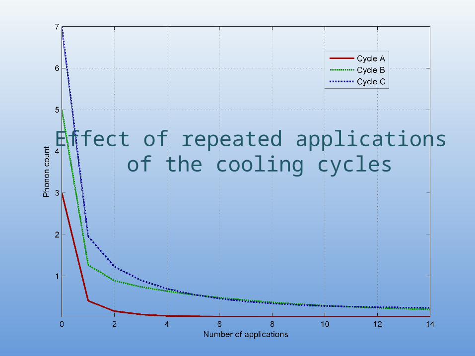
Effect of repeated applicationsof the cooling cycles

Dependence on initial phonon count

25 application of the cooling cycle

Robustness to pulse-length noise

How does a cooling sequence look like?

The unitary transformation

We can do even better• Cycles used were optimized for the impulsive limit

• Stronger coupling meansfaster cooling

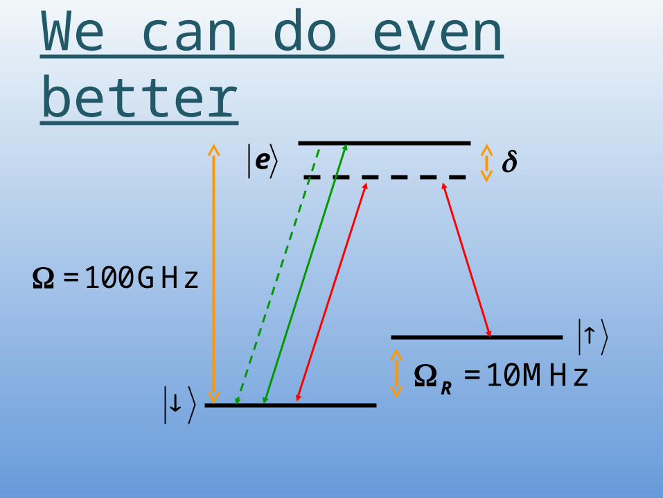
We can do even better

R =10MHz

e

=100GHz

Cycle A Cycle B Cycle C

Initial phonon count 3 5 7

Final phonon count 0.25 1.01 1.69

after 100 cycles 0.0004 0.007 0.025

Cycle duration 0.4 0.3 0.2

No. of X,P pulses 6 3 3

No. of sequences 10 10 10

2

2

2

We can do even better

1 2GHz

/ 2E t

Some additional points

• For linear ion traps, we can cool ions individually – not to the global ground state

• does not apply here, as we’re not measuring energy of an unknown Hamiltonian [Aharonov & Bohm, Phys. Rev. 122 5 (1961) ]

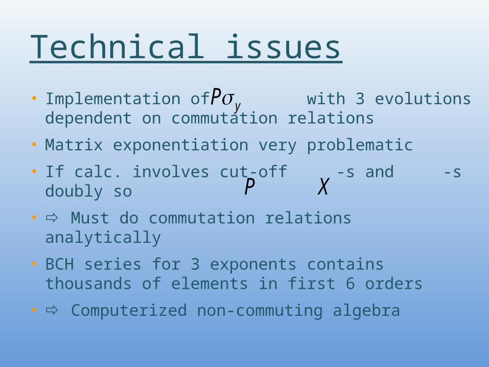
Technical issues• Implementation of with 3 evolutions

dependent on commutation relations

• Matrix exponentiation very problematic

• If calc. involves cut-off -s and -s doubly so

• Must do commutation relations analytically

• BCH series for 3 exponents contains thousands of elements in first 6 orders

• Computerized non-commuting algebra

yP

P X

Superfast cooling

• A novel way of cooling trapped particles

• No upper limit on speed

• Optimized control gives surprisingly good results, even when working with a single coupling

• Applicable to a wide variety of systems

• We will gladly help adapt to your system

Thank you !