Modeling and Mitigation of Interference in Wireless...

Modeling and Mitigation of Interference in Wireless Receivers with Multiple Antennae

Aditya Chopra

PhD Committee:

Prof. Jeffrey Andrews

Prof. Brian L. Evans (Supervisor)

Prof. Robert W. Heath, Jr.

Prof. Elmira Popova

Prof. Haris Vikalo

November 18, 2011 1

The demand for wireless Internet data is predicted to increase 1000× over the next decade

2

0

3.5

7

2010 2011 2012 2013 2014 2015

Mobile Internet Data Demand (Petabytes)

Other Mobile InternetMobile Video

0%

2%

4%

6%

8%

10%

12%

2010 2011 2012 2013 2014 2015

Mobile Internet Traffic as a Percentage of Overall Internet Traffic

2x increase per year!

Introduction | Modeling (CoLo) | Modeling (Dist) | Outage Performance | Receiver Design

Source: Cisco Visual Networking Index Forecast

Wireless communication systems are increasingly using multiple antennae to meet demand

Benefits

Multiplexing Diversity

Multiple data streams are transmitted simultaneously to increase data rate

Antennae with strong channels compensate for

antennae with weak channels to increase reliability

3

Wireless Channel

Transmit Antennae Receive Antennae


101110

11

10

10

A growing mobile user population with increasing wireless data demand leads to interference

4

Interference is also caused by non-communicating source

5

Computational Platform Clocks, amplifiers, busses

Non-communicating devices Microwave ovens Fluorescent bulbs

0 10 20 30

Channel 1

Channel 7

Throughput (Mbps)

LCD OFF

LCD ON

Impact of platform interference from a laptop LCD on wireless throughput (IEEE 802.11g)

[Slattery06]


Interference mitigation has been an active area of research over the past decade

6

I employ a statistical approach to the interference modeling and mitigation problem

Thesis statement Accurate statistical modeling of interference observed by multi-antenna wireless receivers facilitates design of wireless systems with significant improvement in

communication performance in interference-limited networks.

Proposed solution 1. Model statistics of interference in multi-antenna receivers

2. Analyze performance of conventional multi-antenna receivers

3. Develop multi-antenna receiver algorithms using statistical models of interference

7 Introduction | Modeling (CoLo) | Modeling (Dist) | Outage Performance | Receiver Design

A statistical-physical model of interference generation and propagation

Key Features – Co-located receiver antennae ( )

– Interferers are common to all antennae ( ) or exclusive to nth antenna ( )

– Interferers are stochastically distributed in space as a 2D Poisson point process with intensity 𝜆0 ( ), or 𝜆𝑛 ( ) (per unit area)

– Interferer free guard-zone ( ) of radius 𝛿↑

– Power law propagation and fast fading


𝛿↓

1

1

1

1

2

2

2

3 3

A 3-antenna receiver within a Poisson field of interferers

3

n

n

Non-Gaussian distributions have been used in prior work to model single antenna interference statistics

I derive joint statistics of interference observed by multi-antenna receivers

1. Wireless networks with guard zones (Centralized Networks)

2. Wireless networks without guard zones (De-centralized Networks)


Guard Zone Radius (𝛿↓)

Single Antenna Statistics

Characteristic function

Parameters Density Distribution

0 Symmetric Alpha Stable (SAS) [Sousa92]

Φ 𝜔 = 𝑒𝜎𝜔𝛼 𝜎: Dispersion, > 0

𝛼: Index, ∈ (0,2] Not known except 𝛼=2,1,0.5

> 0 Middleton Class A (MCA) [Middleton99] Φ 𝜔 = 𝑒𝐴𝑒

−𝜔2Ω2

𝐴: Impulsive index > 0 Ω: Variance > 0

𝑓 𝑥 = 𝐴𝑚

𝑚! √2𝜋Ω𝑚

∞

𝑚=0𝑒−

𝑥2

𝑚Ω

Gaussian distribution Cauchy distribution Levy distribution

Using the system model, the sum interference at the nth

antenna is expressed as

𝑍𝑛 = 𝐴𝑖0𝑒𝑗𝜙𝑖0𝐻𝑖0,𝑛𝑒

𝑗𝜃𝑖0,𝑛 𝑟𝑖0−𝛾2

𝑖0∈ 𝒮0

+ 𝐴𝑖𝑛𝑒𝑗𝜙𝑖𝑛𝐻𝑖𝑛 𝑒

𝑗𝜃𝑖𝑛 𝑟𝑖𝑛−𝛾2

𝑖𝑛∈ 𝒮𝑛

COMMON INTERFERERS

SOURCE EMISSION

FADING CHANNEL

PATHLOSS

EXCLUSIVE INTERFERERS

10

Network model

Single Ant. Statistics

Multi antenna joint statistics

Common interferers Independent interferers

Decentralized Symmetric Alpha Stable

(SAS)

Isotropic SAS [Ilow98]

Φ 𝐰 = 𝑒𝜎0 𝐰 𝛼

Independent SAS

Φ 𝐰 = 𝑒𝜎𝑛|𝜔𝑛|𝛼

𝑁

𝑛=1

Centralized Middleton Class A (MCA)

×

Independent MCA

Φ 𝐰 = 𝑒𝐴𝑛𝑒−

𝑤2Ω𝑛

2

𝑁

𝑛=1


In networks with guard zones, interference from common interferers exhibits isotropic Middleton Class A statistics

Interference in decentralized networks

Interference in centralized networks


𝛿↓

1

1

1 1

2

2

2

3 3


3

Joint characteristic function Parameters

Φ 𝐰 = 𝑒𝜎0 𝐰 𝛼× 𝑒𝜎𝑛|𝜔𝑛|

𝛼𝑁𝑛=1

𝛼 =4

𝛾,

𝜎𝑛 ∝ 𝜆𝑛

Joint characteristic function Parameters

Φ 𝐰 = 𝑒𝐴0𝑒−

𝐰 2Ω02

× 𝑒𝐴𝑛𝑒−𝑤𝑛

2Ω𝑛2

𝑁𝑛=1

𝐴𝑛 ∝ 𝜆𝑛𝛿↓2 ,

Ω𝑛 ∝ 𝐴𝑛𝛿↓−𝛾

Simulation results indicate a close match between proposed statistical models and simulated interference

12

Tail probability of simulated interference in networks without guard zones

Tail probability of simulated interference in networks with guard zones

PARAMETER VALUES

𝛾 4 𝜆0 = 10−3 , 𝜆𝑛 = 0 (per unit area)

𝛿↓ 1.2 (Distance Units) (w/ GZ)

𝜆0 = 9.5 × 10−4, 𝜆𝑛 = 5 × 10−5 (per unit area)


Tail Probability: ℙ 𝑍1 > 𝜏, 𝑍2 > 𝜏 … 𝑍𝑛 > 𝜏

My framework for multi-antenna interference across co-located antennae results in joint statistics that are

1. Spatially isotropic (common interferers)

2. Spatially independent (exclusive interferers)

3. In a continuum between isotropic and independent (mixture)

for two impulsive distributions

1. Middleton Class A (networks with guard zones)

2. Symmetric alpha stable (networks without guard zones)


In networks without guard zones, antenna separation is incorporated into the system model

Applications – Cooperative MIMO

– Two-hop communication

– Temporal modeling of interference in mobile receivers

Sum interference expression

𝑍1 = 𝐴𝑖0𝑒𝑗𝜙𝑖0𝐻𝑖0,1𝑒

𝑗𝜃𝑖0,1 𝑟𝑖0−𝛾

2𝑖0∈ 𝒮0

+ 𝐴𝑖1𝑒𝑗𝜙𝑖1𝐻𝑖1 𝑒

𝑗𝜃𝑖1 𝑟𝑖1−𝛾

2𝑖1∈ 𝒮1

𝑍2 = 𝐴𝑖0𝑒𝑗𝜙𝑖0𝐻𝑖0,2𝑒

𝑗𝜃𝑖0,2 𝑟𝑖0 −𝑑−𝛾

2𝑖0∈ 𝒮0

+ 𝐴𝑖2𝑒𝑗𝜙𝑖2𝐻𝑖2 𝑒

𝑗𝜃𝑖2 𝑟𝑖2 − 𝑑−𝛾

2𝑖2∈ 𝒮2


Two antennae ( ) and interferers ( ) in a decentralized network

𝑑

1

1 1

1

2

2

2

2 1

2

The extreme scenarios of antenna colocation (𝑑 = 0) and antenna isolation (𝑑 → ∞) are readily resolved

Interference statistics move in a continuum from spatially isotropy to spatial independence as antenna separation increases!

15

Colocated antennae (𝑑 = 0)

Characteristic function of interference:

Φ 𝜔1, 𝜔2 = 𝑒𝜎 𝜔12+𝜔2

2𝛼2

Interference exhibits spatial isotropy

Remote antennae (𝑑 → ∞)

Characteristic function of interference:

Φ 𝜔1, 𝜔2 = 𝑒𝜎 𝜔1𝛼+𝜔2

𝛼

Interference exhibits spatial independence


Interference statistics are approximated using the isotropic-independent statistical mixture framework

Φ 𝜔1,𝜔2 ≈ 𝑒𝜈 𝑑 𝜎 𝜔12+𝜔2

2𝛼2+ 1−𝜈 𝑑 𝜎 𝜔1

𝛼+𝜔2𝛼

16

Weighting function 𝑣(𝑑) for different pathloss exponents (𝛾)

Joint tail probability vs. antenna separation for 𝛾 = 4, 𝜆0 = 10−3, 𝜏 = 3


The framework is used to evaluate communication performance of conventional multi-antenna receivers

Prior Work

System Model Received signal vector 𝐲 = 𝐡𝑠 + 𝐳

𝐡 = ℎ1 ℎ2 ℎ3 ⋯ℎ𝑁𝑇 ~ Rayleigh(𝜎)

𝐳 ~ Isotropic + Independent SAS

Communication performance is evaluated using outage probability

𝑃𝑜𝑢𝑡 𝜃 = ℙ SIR < 𝜃 = ℙ𝑠 2

𝑧′ 2< 𝜃

17

Single Transmit Antenna

Multiple Receive Antennae

ℎ1

ℎ2

ℎ𝑁

𝑠

Introduction | Modeling (CoLo) | Modeling (Dist) |Outage Performance | Receiver Design

Article Wireless System Interference Joint Statistics Performance Metric

[Rajan2011] SIMO SAS Independent Bit Error Rate (BPSK)

[Gao2005] SIMO MCA Indp. / Isotropic Bit Error Rate (BPSK)

[Gao2007] MIMO MCA Independent Bit Error Rate (BPSK)

SIR: Signal-to-Interference Ratio

𝒔 = 𝑠 + 𝐳′

Outage probability of linear combiners

18

+

𝑤1

𝑤𝑁

𝐲 = 𝐡𝑠 + 𝐧 𝐰𝐓𝐲 ⋮

Receiver algorithm Weight vector Outage probability (ℙ 𝑆𝐼𝑅 < 𝜃 )

Equal Gain Combiner 𝐰 = 𝟏𝑁 𝐶0𝜃𝛼2(𝜆0 + 𝜆n𝑁

1−𝛼2)

Maximum Ratio Combiner 𝐰 = 𝐡∗ 𝐶0𝜃𝛼

2𝔼𝐡 𝜆𝑛 𝐡 𝛼

𝛼

𝐡 2𝛼 +

𝜆0

𝐡 22𝛼

Selection Combiner 𝑤𝑛 = ℐ𝒉𝒏=max{𝐡}

𝐶0(𝜆0 + 𝜆𝑛)𝜃𝛼2 −1 𝑛+1

𝑁

𝑛=1

𝑁𝑛

𝑛!


SIR =𝐰𝑇𝐡 𝟐 𝑠 2

𝐰𝑇𝐳 2

×

×

𝐶0 =4 Γ

1 + 𝛼2

Γ 1 −𝛼2

𝔼[𝐴𝛼]

𝜋 cos𝜋𝛼4

Es𝛼𝜎𝑠

𝛼𝜎𝐼𝛼

SIR: Signal-to-Interference Ratio

Outage probability of a genie-aided non-linear combiner

19

SELE

CT

BES

T

⋮

Receiver algorithm Outage probability (ℙ[𝑆𝐼𝑅1 < 𝜃, 𝑆𝐼𝑅2 < 𝜃,⋯ , 𝑆𝐼𝑅𝑁 < 𝜃])

Post Detection Combining 𝐶0 −1 𝑚+1

𝑁

𝑚

(𝑚 + 1 +2𝛾)!

(𝑚 − 1)! sin2𝜋𝛾

𝑁

𝑚=1

𝜃𝛼2 + 𝐶0

𝜋2

𝛾 sin2𝜋𝛾

𝑁 𝜃

𝑁𝛼2

Select antenna stream with best detection SIR Receiver assumes knowledge of SIR at each antenna

SIR𝑛 =ℎ𝑛

𝟐 𝑠 2

𝑧𝑛2


match simulated outage Sim

20

PARAMETER VALUES

Common interferer density(𝜆0) (per unit area) 0.0005

Excl. interferer density(𝜆𝑛) (per unit area) 0.0095

Maximum ratio combining and selection combining receiver performance vs. 𝛼 (N=4)

Outage performance of different combiners vs. number of antennae (𝛾 =6)


(N)

Using communication performance analysis, I design algorithms that outperform conventional receivers

Prior Work

Proposed Receiver Structures

Introduction | Modeling (CoLo) | Modeling (Dist) | Outage Performance | Receiver Design 21

Receiver Type Interference Model Joint Statistics Fading Channel

Filtering Symmetric alpha stable [Gonzales98][Ambike94]

Independent No

Sequence detection, Decision feedback

Gaussian Mixture [Blum00][Bhatia94]

Independent No

Detection Symmetric alpha stable[Rajan10]

Independent Yes

Receiver Type Interference Model

Joint Statistics Fading Channel

Linear filtering SAS Independent/Isotropic Yes

Non-linear filtering SAS Independent/Isotropic Yes

I investigate linear receivers in the presence of alpha stable interference

Linear receivers without channel knowledge Select antenna with strongest mean channel to interference power ratio

Optimal linear receivers with channel knowledge 1. Independent SAS interference

Outage optimal 𝑤𝑛 =

ℎ𝑛∗

ℎ𝑛𝛼−2𝛼−1

, 𝛼 > 1

?, 𝛼 ≤ 1

2. Isotropic SAS interference

Maximum ratio combining is outage optimal

22

Outage of optimal linear combiner in spatially independent interference (𝛼=1.3)


(N)

I propose sub-optimal non-linear receivers for impulsive interference

‘Deviation’ in an antenna output 𝑦𝑛 is defined as

Δ𝑛 = |𝑦𝑛| −median{ 𝐲 }

Proposed diversity combiners

1. Hard-limiting combiner

𝑤𝑛 = 𝟏Δ𝑛<𝑇ℎ𝑛∗

2. Soft-limiting combiner

𝑤𝑛 = 𝑒−𝐴Δ𝑛ℎ𝑛∗

23

0 1 2 3 4

0

1

Ante

nna

Weig

ht

(w)

Deviation (

Hard Limiting (T=1)

Soft Limiting (A=1)


Proposed diversity combiners exhibit better outage performance compared to conventional combiners

24

Parameter values

Pathloss coefficient (𝛾) 4

Guard- zone radius (𝛿↓) (Unit Distance)

0

Common interferer density(𝜆0) (per unit area)

0.0005

Exclusive interferer density(𝜆𝑛) (per unit area)

0.0095

HL combiner parameter (𝑇) 1

SL combiner parameter (𝐴) 2


10x improvement in outage probability

Joint interference statistics across separate antennae can also improve cooperative reception strategies

System Model Performance-Cost tradeoff A distant base-station transmits a signal to the destination receiver ( ) surrounded by interferers ( ) and cooperative receivers ( )

Which cooperative receiver should be selected to assist in signal reception?

25

Antenna Separation (Distance Units) 0 ∞

Outage Probability

Power Cost


Total cost is evaluated using a re-transmission based model

Optimal Antenna Separation

𝑘th-Nearest Neighbor Selection 𝑑𝑘~𝐷𝑘 is the random variable describing

the location of the k-th nearest neighbor

26

𝑑∗ = arg min𝑑>0

𝐶 𝑑 × 𝑃𝑜𝑢𝑡 𝑑

1 − 𝑃𝑜𝑢𝑡(𝑑)

Optimal cooperative antenna location

Cost per re-transmission

Expected re-transmissions

𝑘∗ = arg min𝑑>0

𝔼𝑑𝑘 𝐶 𝑑𝑘 × 𝑃𝑜𝑢𝑡 𝑑𝑘

1 − 𝑃𝑜𝑢𝑡 𝑑𝑘

Optimal k-th nearest neighbor

Expected Cost of k-th re-transmission

Cooperative antenna power usage vs. separation. Power usage increases as 𝑑𝛾 (𝛾 = 6) with 10mW fixed overhead and usage of 150mW at 50 distance units.

10% Outage probability per individual antenna.

In conclusion, the contributions of my dissertation are 1. A framework for modeling multi-antenna interference

– Interference statistics are mix of spatial isotropy and spatial independence

2. Statistical modeling of multi-antenna interference

– Co-located antennae in networks without guard zones – Two geographically separate antennae in networks with guard zones

3. Outage performance analysis of conventional receivers in networks without

guard zones – Accurate outage probability expressions inform receiver design

4. Design of receiver algorithms with improved performance in impulsive

interference – Order of magnitude reduction in outage probability compared to linear

receivers – 80% reduction in power by using physically separate antennae

27

Future work Statistical Modeling • Non-Poisson distribution of interferer locations • >2 physically separate antennae in a field of interferers • Physically separate antennae in a centralized network • Temporal modeling of interference statistics with correlated

fields of randomly distributed interferers

Performance Analysis • Performance analysis of multi-antenna wireless networks

Receiver Design • Closed form expressions and bounds on performance of non-

linear receivers • Incorporate interference modeling into conventional relaying

strategies

28

Journal Papers 1. A. Chopra and B. L. Evans, ̀ `Outage Probability for Diversity Combining in Interference-Limited Channels'', IEEE

Transactions on Wireless Communications, submitted Sep. 14, 2011

2. A. Chopra and B. L. Evans, ̀ `Joint Statistics of Radio Frequency Interference in Multi-Antenna Receivers'', IEEE Transactions on Signal Processing, accepted with minor mandatory changes.

3. A. Chopra and B. L. Evans, ̀ `Design of Sparse Filters for Channel Shortening'', Journal of Signal Processing Systems, May 2011, 14 pages, DOI 10.1007/s11265-011-0591-0

Conference Papers 1. A. Chopra and B. L. Evans, ̀ `Design of Sparse Filters for Channel Shortening'', Proc. IEEE Int. Conf. on Acoustics,

Speech, and Signal Proc., Mar. 14-19, 2010, Dallas, Texas USA.

2. A. Chopra, K. Gulati, B. L. Evans, K. R. Tinsley, and C. Sreerama, ̀ `Performance Bounds of MIMO Receivers in the Presence of Radio Frequency Interference'', Proc. IEEE Int. Conf. on Acoustics, Speech, and Signal Proc., Apr. 19-24, 2009, Taipei, Taiwan.

3. K. Gulati, A. Chopra, B. L. Evans, and K. R. Tinsley, ̀ `Statistical Modeling of Co-Channel Interference'', Proc. IEEE Int. Global Communications Conf., Nov. 30-Dec. 4, 2009, Honolulu, Hawaii.

4. K. Gulati, A. Chopra, R. W. Heath, Jr., B. L. Evans, K. R. Tinsley, and X. E. Lin, ̀ `MIMO Receiver Design in the Presence of Radio Frequency Interference'', Proc. IEEE Int. Global Communications Conf., Nov. 30-Dec. 4th, 2008, New Orleans, LA USA.

5. A. G. Olson, A. Chopra, Y. Mortazavi, I. C. Wong, and B. L. Evans, ̀ `Real-Time MIMO Discrete Multitone Transceiver Testbed'', Proc. Asilomar Conf. on Signals, Systems, and Computers, Nov. 4-7, 2007, Pacific Grove, CA USA.

In preparation 1. A. Chopra and B. L. Evans, ̀ `Joint Statistics of Interference Across Two Separate Antennae''

29

References RFI Modeling 1. -Gaussian noise models in signal processing for

telecommunications: New methods and results for Class A and Class B noise IEEE Trans. Info. Theory, vol. 45, no. 4, pp. 1129-1149, May 1999.

2.J. Ilow and D . Hatzinakos -stable noise modeling in a Poisson field of interferers or scatterers IEEE Trans. on Signal Proc., vol. 46, no. 6, pp. 1601-1611, Jun. 1998.

3.IEEE Trans. on Info. Theory, vol. 38, no. 6, pp.

1743 1754, Nov. 1992. 4.X. Yang and A. Petropulu -channel interference modeling and analysis in a

IEEE Trans. on Signal Proc., vol. 51, no. 1, pp. 64 76, Jan. 2003.

5. Cisco visual networking index: Global mobile data traffic forecast update, 2010 - 2015. Technical report, Feb. 2011.

6. John P. Nolan. Multivariate stable densities and distribution functions: general and elliptical case. Deutsche Annual Fall Conference, 2005.

30

Performance Analysis 1. Ping Gao and C. Tepedelenlioglu. Space-time coding over fading

channels with impulsive noise. IEEE Transactions on Wireless Communications, 6(1):220 229, Jan. 2007.

2. A. Rajan and C. Tepedelenlioglu. Diversity combining over Rayleigh fading channels with symmetric alpha-stable noise. IEEE Transactions on Wireless Communications, 9(9):2968 2976, 2010.

3. S. Niranjayan and N. C. Beaulieu. The BER optimal linear rake receiver for signal detection in symmetric alpha-stable noise. IEEE Transactions on Communications, 57(12):3585 3588, 2009.

4. C. Tepedelenlioglu and Ping Gao. On diversity reception over fading channels with impulsive noise. IEEE Transactions on Vehicular Technology, 54(6):2037 2047, Nov. 2005.

5. G. A. Tsihrintzis and C. L. Nikias. Performance of optimum and suboptimum receivers in the presence of impulsive noise modeled as an alpha stable process. IEEE Transactions on Communications, 43(234):904 914, 1995.

31

Receiver Design 1.A.

Interference Environment- IEEE Trans. Comm., vol. 25, no. 9, Sep. 1977

2.J.G. Gonzalez and G.R. ArceImpulsive- IEEE Trans. on Signal Proc., vol. 49, no. 2, Feb 2001

3.S. Ambike, J. Ilow, and D. Hatzinakosmixture of Gaussian noise and impulsive noise modelled as an alpha-stable

IEEE Signal Proc. Letters, vol. 1, pp. 55 57, Mar. 1994. 4.O. B. S. Ali, C. Cardinal, and F. Gagnon. Performance of optimum combining in

a Poisson field of interferers and Rayleigh fading channels. IEEE Transactions on Wireless Communications, 9(8):2461 2467, 2010.

5.Andres Altieri, Leonardo Rey Vega, Cecilia G. Galarza, and Pablo Piantanida. Cooperative strategies for interference-limited wireless networks. In Proc. IEEE International Symposium on Information Theory, pages 1623 1627, 2011.

6. Y. Chen and R. S. Blum. Efficient algorithms for sequence detection in non-Gaussian noise with intersymbol interference. IEEE Transactions on Communications, 48(8):1249 1252, Aug. 2000.

32

about me Member of the Wireless Networking and Communications Group at The University of Texas at Austin since 2006.

Completed projects

Currently active projects

33

ADSL testbed (Oil & Gas) 2 x 2 wired multicarrier communications testbed using PXI hardware, x86 processor, real-time operating system and LabVIEW

Spur modeling/mitigation (NI) Detect and classify spurious signals; fixed and floating-point algorithms to mitigate spurs

Interference modeling and mitigation (Intel)

Statistical models of interference; receiver algorithms to mitigate interference; MATLAB toolbox

Impulsive noise mitigation in OFDM (NI)

Non-parametric interference mitigiation for wireless OFDM receivers using PXI hardware, FPGAs, and LabVIEW

Powerline communications (TI, Freescale, SRC)

Modeling and mitigating impulsive noise; building multichannel multicarrier communications testbed using PXI hardware, x86 processor, real-time operating system, LabVIEW

Interference mitigation has been an active area of research over the past decade

INTERFERENCE MITIGATION STRATEGY

LIMITATIONS

Hardware design

- Receiver shielding Does not mitigate interference from

devices using same spectrum

Network planning

- Resource allocation - Basestation coordination - Partial frequency re-use

Requires user coordination Slow updates

Receiver algorithms

- Interference cancellation - Interference alignment - Statistical interference mitigation

Require user coordination and channel state information

Statistical methods require accurate interference models

Introduction | Modeling (CoLo) | Modeling (Dist) | Outage Performance | Receiver Design 34

Interference Mitigation Techniques

35

Interference alignment

36

Interference cancellation

J. G. Andrews, IEEE Wireless Communications Magazine, Vol. 12, No. 2, pp. 19-29, April 2005

37

Femtocell Networks

V. Chandrasekhar, J. G. Andrews and A. Gatherer, "Femtocell Networks: a Survey", IEEE Communications Magazine, Vol. 46, No. 9, pp. 59-67, September 2008

Wireless Networking and Communications Group 38

Spectrum Occupied by Typical Standards

39

39

Standard Carrier (GHz)

Wireless Networking

Interfering Clocks and Busses

Bluetooth 2.4 Personal Area

Network Gigabit Ethernet, PCI Express Bus,

LCD clock harmonics

IEEE 802. 11 b/g/n

2.4 Wireless LAN

(Wi-Fi) Gigabit Ethernet, PCI Express Bus,

LCD clock harmonics

IEEE 802.16e

2.5–2.69 3.3–3.8

5.725–5.85

Mobile Broadband (Wi-Max)

PCI Express Bus, LCD clock harmonics

IEEE 802.11a

5.2 Wireless LAN

(Wi-Fi) PCI Express Bus,

LCD clock harmonics

Impact of LCD on 802.11g

Pixel clock 65 MHz

LCD Interferers and 802.11g center frequencies

40

40

LCD Interferers

802.11g Channel

Center Frequency

Difference of Interference from Center Frequencies

Impact

2.410 GHz Channel 1 2.412 GHz ~2 MHz Significant

2.442 GHz Channel 7 2.442 GHz ~0 MHz Severe

2.475 GHz Channel 11 2.462 GHz ~13 MHz Just outside Ch. 11. Impact minor

Measured Data

25 radiated computer platform RFI data sets from Intel each with 50,000 samples taken at 100 MSPS

41

0 5 10 15 20 250

0.05

0.1

0.15

0.2

0.25

0.3

0.35

0.4

Measurement Set

Kullb

ack-L

eib

ler

div

erg

ence

Symmetric Alpha Stable

Middleton Class A

Gaussian Mixture Model

Gaussian

Single Antenna RFI Models

Model Name Key Features

Symmetric alpha stable [Sousa,1992]

[Ilow & Hatzinakos,1998]

• Models wireless ad hoc networks, computational platform

noise • No closed form distribution function (except 𝛼 = 1,2) • Unbounded variance (generally 𝐸 𝑋𝛼 → ∞)

Middleton Class A [Middleton, 1979, 1999]

• Models wireless networks with guard zones and interferers

in a finite area around receiver [Gulati, Chopra, Evans & Tinsley, 2009]

• Model incorporates thermal noise present at receiver • Special case of the Gaussian mixture distribution

Gaussian mixture distribution

• Models wireless networks with hotspots, femtocell

networks [Gulati, Evans, Andrews & Tinsley, 2009]

Introduction |RFI Modeling | Performance Analysis | Receiver Design | Summary 42

Single Antenna RFI Models

• Symmetric alpha stable distribution [Sousa,1992]

– Characteristic function:

Φ 𝜔 = 𝑒−𝜎|𝜔|𝛼

• Middleton Class A distribution [Middleton, 1977, 1999]

Amplitude distribution:

• Gaussian mixture distribution – Amplitude distribution:

Parameter Range 𝛼 [0,2] 𝜎 (0,∞)

Parameter Range 𝐴 [0,2] Γ (0,∞) 𝜎 (0,∞)

Parameter Range 𝑝1, 𝑝2, ⋯ [0,1]

𝜎1, 𝜎2, ⋯ (0,∞)


Two-Antenna RFI Generation Model • Key model characteristics

– Correlated interferer field observed by receive antennas

– Inter-antenna distances insignificant compared to antenna-interferer distances

• Sum interference in two-antenna receiver

𝐘1 = 𝐵𝑖𝑒𝑗𝜃𝑖𝑟𝑖

−𝛾/2ℎ𝑖𝑒

𝑗𝜙𝑖

𝑖∈Π0

+ 𝐵𝑖′𝑒𝑗𝜃

𝑖′𝑟𝑖′−𝛾/2

ℎ𝑖′𝑒𝑗𝜙

𝑖′

𝑖′∈Π1

𝐘2 = 𝐵𝑖𝑒𝑗𝜃𝑖𝑟𝑖


𝑗𝜙𝑖

𝑖∈Π0




𝑖′

𝑖′∈Π2

– Π0 denotes set of interferers observed by both antennas (intensity 𝜆0)

– Π1, Π2 denote interferers observed at antenna 1 and 2 respectively (intensity 𝜆1, 𝜆2)

INTERFERER TO ANTENNA 2 INTERFERER TO ANTENNA 1 COMMON INTERFERER


Multi-Antenna RFI Generation Model • Spatially correlated interferer fields in 𝑁𝑅-antenna receiver

– 2𝑁𝑅– 1 i.i.d. interferer sets

– Sum interference from 2𝑁𝑅−1 sets at each antenna

• Proposed model extension to 𝑁𝑅-antenna receiver

– Two categories of interferers

– Sum interference from 2 sets at each antenna

• Sum interference in 𝑁𝑅-antenna receiver

𝐘𝑘 = 𝐵𝑖𝑒𝑗𝜃𝑖𝑟𝑖


𝑗𝜙𝑖

𝑖∈Π0




𝑖′

𝑖′∈Π𝑘

– Π0 is set of interferers common to all receive antennas (intensity 𝜆0)

– Π𝑘 is set of interferers observed by receive antenna 𝑘 (intensity 𝜆𝑘)

Emissions lead to RFI in all antennas Emissions lead to RFI in one antenna


Existing Models of Multi-Antenna RFI

Model Name Key Features

Symmetric alpha stable (isotropic)

[Ilow & Hatzinakos,1998]

• Models spatially dependent RFI generated from single set of interferers observed by all receive antennas

• No closed form distribution function (except 𝛼 = 1,2) • Unbounded variance (generally 𝐸 𝑋𝛼 → ∞)

Multidimensional Class A Models I − III [Delaney, 1995]

• Multidimensional extension of Middleton class A distribution, no statistical derivation

• Different statistical distributions required to reflect spatial dependence/independence in RFI

Bivariate class A distribution [McDonald & Blum, 1997]

• Approximate distribution based on statistical-physical derivation

• Models RFI observed at two receive antennas only • Spatially dependent RFI

Temporal second-order alpha stable model

[Yang & Petropulu, 2003]

• Models second-order temporal statistics of co-channel interference

• Assumes temporal correlation in interferer fields


Extension type Amplitude distribution

Spatially independent

Isotropic

Statistical Models for Multi-Antenna RFI

• Multidimensional symmetric alpha stable distribution [Ilow & Hatzinakos, 1998]

• Multidimensional Class A distribution [Delaney, 1995]

Extension type Characteristic function

Spatially independent Φ 𝜔 = 𝑒− 𝜎𝑛|𝜔𝑛|𝛼𝑁𝑅

𝑛=1

Isotropic Φ 𝜔 = 𝑒−𝜎||𝐰||𝛼


Statistical Models for Multi Antenna RFI

• Physical model of RFI for 2 antenna systems – Amplitude distribution [McDonald & Blum, 1997]

Parameter Range 𝐴 [0,2]

Γ1, Γ2 (0,∞) 𝜅 [0,1]


KL divergence

49

Interference in separate antennae

50

Wireless Networking and Communications Group

Homogeneous Spatial Poisson Point Process

51


Poisson Field of Interferers

52

Applied to wireless ad hoc networks, cellular networks

Closed Form Amplitude Distribution

Model Interference Region Key Prior Work

Symmetric Alpha Stable

Spatial Entire plane

[Sousa, 1992] [Ilow & Hatzinakos, 1998] [Yang & Petropulu, 2003]

Middleton Class A Spatio-temporal Finite area [Middleton, 1977, 1999]

Other Interference Statistics – closed form amplitude distribution not derived

Statistics Interference Region Key Prior Work

Moments Spatial Finite area [Salbaroli & Zanella, 2009]

Characteristic Function Spatial Finite area [Win, Pinto & Shepp,2009]

Isotropic SAS

53

Independent SAS

54

Mixture SAS

55

Threshold selection with 𝛼 =2

3

56

Threshold selection with 𝛼 =4

3

57

Parameter Estimators for Alpha Stable

58

58

Return


Gaussian Mixture vs. Alpha Stable

59

• Gaussian Mixture vs. Symmetric Alpha Stable

Gaussian Mixture Symmetric Alpha Stable

Modeling Interferers distributed with Guard zone around receiver (actual or virtual due to PL)

Interferers distributed over entire plane

Pathloss Function

With GZ: singular / non-singular Entire plane: non-singular

Singular form

Thermal Noise

Easily extended (sum is Gaussian mixture)

Not easily extended (sum is Middleton Class B)

Outliers Easily extended to include outliers Difficult to include outliers


RFI Mitigation in SISO Systems

60

60

Computer Platform Noise Modelling

Evaluate fit of measured RFI data to noise models • Middleton Class A model • Symmetric Alpha Stable

Parameter Estimation

Evaluate estimation accuracy vs complexity tradeoffs

Filtering / Detection Evaluate communication performance vs complexity tradeoffs • Middleton Class A: Correlation receiver, Wiener filtering,

and Bayesian detector • Symmetric Alpha Stable: Myriad filtering, hole punching,

and Bayesian detector

Mitigation of computational platform noise in single carrier, single antenna systems [Nassar, Gulati, DeYoung, Evans & Tinsley, ICASSP 2008, JSPS 2009]

Return


Filtering and Detection

61

61

Pulse Shaping

Pre-Filtering Matched

Filter Detection

Rule

Impulsive Noise

Middleton Class A noise Symmetric Alpha Stable noise

Filtering Wiener Filtering (Linear)

Detection Correlation Receiver (Linear) Bayesian Detector

[Spaulding & Middleton, 1977]

Small Signal Approximation to Bayesian detector [Spaulding & Middleton, 1977]

Filtering Myriad Filtering

Optimal Myriad [Gonzalez & Arce, 2001]

Selection Myriad

Hole Punching [Ambike et al., 1994]

Detection Correlation Receiver (Linear) MAP approximation

[Kuruoglu, 1998]

Assumption Multiple samples of the received signal are available • N Path Diversity [Miller, 1972] • Oversampling by N [Middleton, 1977]

Return


Results: Class A Detection

62

62

Pulse shape Raised cosine

10 samples per symbol 10 symbols per pulse

Channel A = 0.35

= 0.5 × 10-3

Memoryless

Method Comp. Complexity

Detection Perform.

Correl. Low Low

Wiener Medium Low

Bayesian S.S. Approx.

Medium High

Bayesian High High -35 -30 -25 -20 -15 -10 -5 0 5 10 1510

-5

10-4

10-3

10-2

10-1

100

SNR

Bit

Err

or

Rate

(B

ER

)

Correlation Receiver

Wiener Filtering

Bayesian Detection

Small Signal Approximation

Communication Performance Binary Phase Shift Keying


Results: Alpha Stable Detection

63

63

Use dispersion parameter g in place of noise variance to generalize SNR

Method Comp. Complexity

Detection Perform.

Hole Punching

Low Medium

Selection Myriad

Low Medium

MAP Approx.

Medium High

Optimal Myriad

High Medium

-10 -5 0 5 10 15 20

10-2

10-1

100

Generalized SNR (in dB)

Bit

Err

or

Rate

(B

ER

)

Matched Filter

Hole Punching

MAP

Myriad

Communication Performance Same transmitter settings as previous slide Return


RFI Mitigation in 2x2 MIMO Systems

64

64

RFI Modeling • Evaluated fit of measured RFI data to the bivariate Middleton Class A model [McDonald & Blum, 1997]

• Includes noise correlation between two antennas

Parameter Estimation

• Derived parameter estimation algorithm based on the method of moments (sixth order moments)

Performance Analysis

• Demonstrated communication performance degradation of conventional receivers in presence of RFI

• Bounds on communication performance [Chopra , Gulati, Evans, Tinsley, and Sreerama, ICASSP 2009]

Receiver Design • Derived Maximum Likelihood (ML) receiver • Derived two sub-optimal ML receivers with reduced

complexity

2 x 2 MIMO receiver design in the presence of RFI [Gulati, Chopra, Heath, Evans, Tinsley & Lin, Globecom 2008]

Return

65 Wireless Networking and Communications Group

Bivariate Middleton Class A Model

• Joint spatial distribution

Parameter Description Typical Range

Overlap Index. Product of average number of emissions per second and mean duration of typical emission

Ratio of Gaussian to non-Gaussian component intensity at each of the two antennas

Correlation coefficient between antenna observations

Return


Results on Measured RFI Data

• 50,000 baseband noise samples represent broadband interference

Estimated Parameters

Bivariate Middleton Class A

Overlap Index (A) 0.313

2D- KL Divergence

1.004

Gaussian Factor (1) 0.105

Gaussian Factor (2) 0.101

Correlation (k) -0.085

Bivariate Gaussian

Mean (µ) 0

2D- KL Divergence

1.6682

Variance (s1) 1

Variance (s2) 1

Correlation (k) -0.085

-4 -3 -2 -1 0 1 2 3 40

0.2

0.4

0.6

0.8

1

1.2

1.4

Noise amplitude

Pro

ba

bility D

en

sity F

un

ctio

n

Measured PDF

Estimated MiddletonClass A PDF

Equi-powerGaussian PDF

Marginal PDFs of measured data compared with estimated model densities

68

• 2 x 2 MIMO System

• Maximum Likelihood (ML) receiver

• Log-likelihood function


System Model

Sub-optimal ML Receivers approximate

Return


Sub-Optimal ML Receivers 69

• Two-piece linear approximation

• Four-piece linear approximation

-5 -4 -3 -2 -1 0 1 2 3 4 5

0

0.5

1

1.5

2

2.5

3

3.5

4

4.5

5

z

Ap

pro

xm

atio

n o

f (z

)

(z)

1(z)

2(z)

chosen to minimize Approximation of

Return


Results: Performance Degradation

• Performance degradation in receivers designed assuming additive Gaussian noise in the presence of RFI

-10 -5 0 5 10 15 2010

-5

10-4

10-3

10-2

10-1

100

SNR [in dB]

Vecto

r S

ym

bol E

rror

Rate

SM with ML (Gaussian noise)

SM with ZF (Gaussian noise)

Alamouti coding (Gaussian noise)

SM with ML (Middleton noise)

SM with ZF (Middleton noise)

Alamouti coding (Middleton noise)

Simulation Parameters • 4-QAM for Spatial Multiplexing (SM)

transmission mode • 16-QAM for Alamouti transmission

strategy • Noise Parameters:

A = 0.1, 1= 0.01, 2= 0.1, k = 0.4

Severe degradation in communication performance in

high-SNR regimes

Return


Results: RFI Mitigation in 2 x 2 MIMO

71

-10 -5 0 5 10 15 20

10-3

10-2

10-1

SNR [in dB]

Vecto

r S

ym

bol E

rror

Rate

Optimal ML Receiver (for Gaussian noise)

Optimal ML Receiver (for Middleton Class A)

Sub-Optimal ML Receiver (Four-Piece)

Sub-Optimal ML Receiver (Two-Piece)

71

A Noise

Characteristic Improve

-ment

0.01 Highly Impulsive ~15 dB

0.1 Moderately Impulsive

~8 dB

1 Nearly Gaussian ~0.5 dB

Improvement in communication performance over conventional Gaussian ML receiver at symbol

error rate of 10-2

Communication Performance (A = 0.1, 1= 0.01, 2= 0.1, k = 0.4)

Return


Results: RFI Mitigation in 2 x 2 MIMO

72

72

Complexity Analysis

Re

ceiv

er

Qu

adra

tic

Form

s

Exp

on

en

tial

Co

mp

aris

on

s

Gaussian ML M2 0 0

Optimal ML 2M2 2M2 0

Sub-optimal ML (Four-Piece)

2M2 0 2M2

Sub-optimal ML (Two-Piece)

2M2 0 M2

Complexity Analysis for decoding M-level QAM modulated signal

Communication Performance (A = 0.1, 1= 0.01, 2= 0.1, k = 0.4)

-10 -5 0 5 10 15 20

10-3

10-2

10-1

SNR [in dB]

Vecto

r S

ym

bol E

rror

Rate

Optimal ML Receiver (for Gaussian noise)

Optimal ML Receiver (for Middleton Class A)

Sub-Optimal ML Receiver (Four-Piece)

Sub-Optimal ML Receiver (Two-Piece)

Return

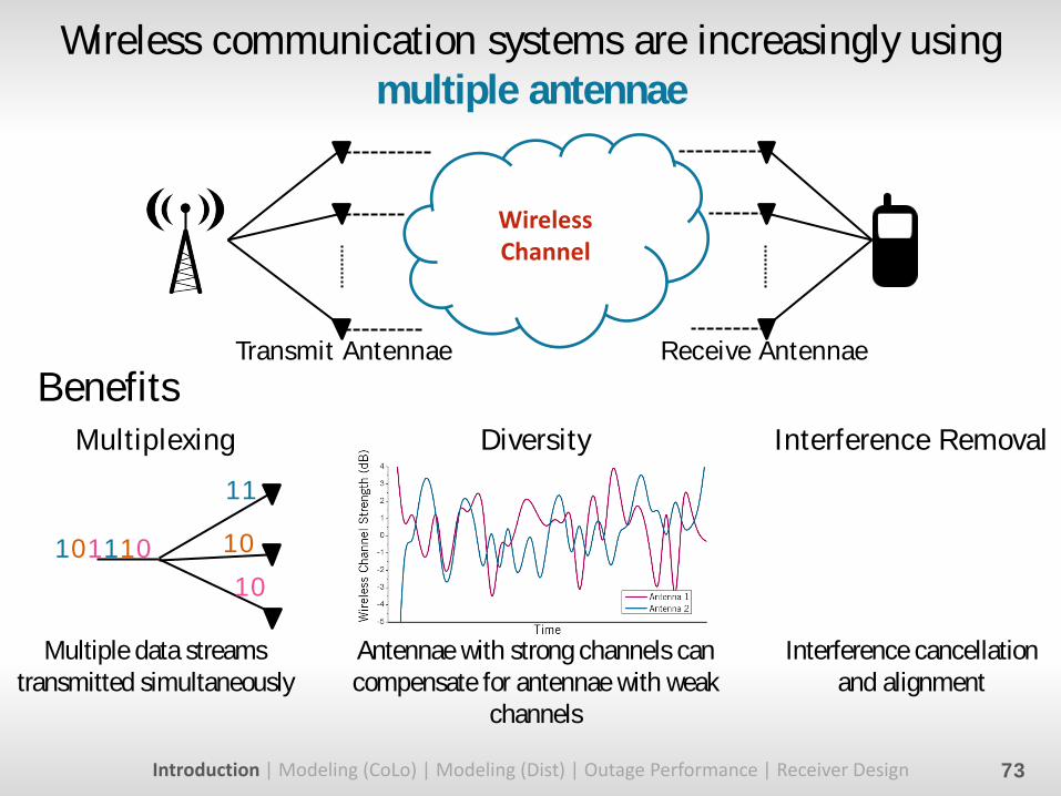
Wireless communication systems are increasingly using multiple antennae

Benefits

73

Multiplexing Diversity Interference Removal

Multiple data streams transmitted simultaneously

Antennae with strong channels can compensate for antennae with weak

channels

Interference cancellation and alignment

Wireless Channel

Transmit Antennae Receive Antennae


101110

11

10

10

Interference statistics in networks without guard zones are a mix of isotropic and i.i.d. alpha stable

Joint characteristic function

Φ 𝑤 = 𝑒𝜎0 𝐰 𝛼× 𝑒𝜎𝑛|𝜔𝑛|

𝛼𝑁𝑛=1

𝛼 =4

𝛾, 𝜎𝑛 ∝ 𝜆𝑛

and interference statistics in networks with guard zones are a mix of isotropic and i.i.d. Middleton Class A

Joint characteristic function

Φ 𝑤 = 𝑒𝐴0𝑒−

𝐰 2Ω02

× 𝑒𝐴𝑛𝑒−𝑤𝑛

2Ω𝑛2

𝑁𝑛=1 𝐴𝑛 ∝ 𝜆𝑛𝛿↓

2 ,Ω𝑛 ∝ 𝐴𝑛𝛿↓−𝛾


𝛿↓

1

1

1 1

2

2

2

3 3


3

Modeling and Mitigation of Interference in Wireless...

Documents

Transcript of Modeling and Mitigation of Interference in Wireless...