Interference Mitigation in Wireless Communications

A ThesisPresented to

The Academic Faculty

by

Kihong Kim

In Partial Fulfillmentof the Requirements for the Degree

Doctor of Philosophy

School of Electrical and Computer EngineeringGeorgia Institute of Technology

December 2005

Interference Mitigation in Wireless Communications

Approved by:

Professor Gordon L. Stuber,Advisor and Committee ChairElectrical and Computer Engineering

Professor Ye (Geofferey) LiElectrical and Computer Engineering

Professor Mary Ann Ingram,Electrical and Computer Engineering

Professor Douglas B. Williams,Electrical and Computer Engineering

Professor Alfred Andrew,Mathematics

Date Approved: 23 August 2005

To,

My wife, Yeongseon, my daughter, Jeeyoon

and our parents

for their love for all these years.

iii

ACKNOWLEDGEMENTS

This dissertation could not be completed without influences from several individuals, to

whom I am grateful for their contributions, direct or indirect, to the completion of this

research.

First and foremost, I would like to acknowledge a tremendous debt of gratitude towards

my advisor, Prof. Gordon Stuber, whose patience, understanding, and guidance to me

cannot be overstated. In addition to his academic supervision, I am also grateful for his

financial support throughout my study. Most of all, I have learned a lot more than research

work through his loyalty to integrity as an academic professional.

Next, I thank the reading committee members of my dissertation committee, Prof. Ye

(Geofferey) Li and Prof. Mary Ann Ingram for their time, effort, and valuable suggestions

necessary to complete this work. I also extend my thank to Prof. Douglas Williams and

Prof. Alfred Andrew for having dedicated their valuable time to participate my dissertation

committee, and having provided insightful comments and feedbacks for this research.

I thank all other members of Wireless Systems Laboratory (WSL), past and present,

Dr. Jinsoup Joung, Dr. Hasung Kim, Heewon Kang, Joon Beom Kim, Chirag Patel, Alenka

Zajic, and Qing Zhao, in no particular order, for all the time and discussions we shared

during my stay at WSL. Especially, I give thanks to Dr. Apurva Mody. His optimism in

academic and personal life has always made me focus on the light at the end of the tunnel.

I also thank Dr. Tom Pratt and Galib Asadullah for their dedicated collaboration on the

GSM project.

Lastly, I owe a debt of gratitude to my family for their love, support, and sacrifice along

the path of my academic pursuits. For all this and much more, I dedicate this thesis to

them.

Thank God for showing me the beginning and the end of a segment of the path of my

life.

iv

TABLE OF CONTENTS

DEDICATION . . . . . . . . . . . . . . . . . . . . . . . . . . . . . . . . . . . . . . iii

ACKNOWLEDGEMENTS . . . . . . . . . . . . . . . . . . . . . . . . . . . . . . iv

LIST OF TABLES . . . . . . . . . . . . . . . . . . . . . . . . . . . . . . . . . . . ix

LIST OF FIGURES . . . . . . . . . . . . . . . . . . . . . . . . . . . . . . . . . . x

LIST OF ABBREVIATIONS . . . . . . . . . . . . . . . . . . . . . . . . . . . . . xiii

SUMMARY . . . . . . . . . . . . . . . . . . . . . . . . . . . . . . . . . . . . . . . . xvi

I INTRODUCTION . . . . . . . . . . . . . . . . . . . . . . . . . . . . . . . . . 1

1.1 Problem and Solution . . . . . . . . . . . . . . . . . . . . . . . . . . . . . . 3

1.1.1 Interference Cancellation in Asynchronous Slow FH Networks . . . 4

1.1.2 Joint Detection Interference Rejection Combining TDMA Receiver 5

1.1.3 CCI Mitigation in Space-Time MIMO Communication Systems . . 6

1.2 Thesis Outline . . . . . . . . . . . . . . . . . . . . . . . . . . . . . . . . . . 7

II BACKGROUND . . . . . . . . . . . . . . . . . . . . . . . . . . . . . . . . . . 9

2.1 Interference in Wireless Communications . . . . . . . . . . . . . . . . . . . 9

2.1.1 Propagation Channels . . . . . . . . . . . . . . . . . . . . . . . . . 9

2.1.2 Intersymbol Interference (ISI) . . . . . . . . . . . . . . . . . . . . . 10

2.1.3 Co-Channel and Adjacent-Channel Interference (CCI and ACI) . . 10

2.1.4 Interference in ISM Bands . . . . . . . . . . . . . . . . . . . . . . . 11

2.2 Interference Mitigation Techniques . . . . . . . . . . . . . . . . . . . . . . 11

2.2.1 Frequency Reuse and Multiple Access . . . . . . . . . . . . . . . . . 12

2.2.2 Adaptive Filtering . . . . . . . . . . . . . . . . . . . . . . . . . . . 13

2.2.3 Spatio-Temporal Interference Mitigation . . . . . . . . . . . . . . . 15

2.2.4 Multiuser Detection . . . . . . . . . . . . . . . . . . . . . . . . . . . 19

2.3 Packet-Level Performance in Wireless Communication . . . . . . . . . . . 21

2.3.1 AWGN Channels . . . . . . . . . . . . . . . . . . . . . . . . . . . . 21

2.3.2 Time-Varying Fading Channels . . . . . . . . . . . . . . . . . . . . 21

2.3.3 Uncoordinated Wireless Packet Networks . . . . . . . . . . . . . . . 23

2.4 CCI and Channel Capacity in MIMO Systems . . . . . . . . . . . . . . . . 24

v

2.4.1 Channel State Information (CSI) and Power Allocation . . . . . . . 24

2.4.2 Antenna Subset Selection in MIMO Systems . . . . . . . . . . . . . 25

2.4.3 Space-Time MIMO Signalling . . . . . . . . . . . . . . . . . . . . . 26

2.4.4 Receiver Structures for Space-Time MIMO Systems . . . . . . . . . 27

III INTERFERENCE MITIGATION IN ASYNCHRONOUS SLOW FRE-QUENCY HOPPING BLUETOOTH NETWORKS . . . . . . . . . . . 29

3.1 Introduction . . . . . . . . . . . . . . . . . . . . . . . . . . . . . . . . . . . 29

3.2 Signal and Interference Model for Asynchronous SFH Bluetooth Networks 31

3.2.1 Signal Model of Bluetooth System . . . . . . . . . . . . . . . . . . . 31

3.2.2 Channel and Co-channel Interference Model . . . . . . . . . . . . . 33

3.2.3 IC-DDF Maximal Likelihood (ML) Receiver . . . . . . . . . . . . . 34

3.2.4 Simplified RLS Channel Estimation . . . . . . . . . . . . . . . . . . 36

3.3 Analysis of System Level Performance . . . . . . . . . . . . . . . . . . . . 36

3.3.1 Packet Error Probability . . . . . . . . . . . . . . . . . . . . . . . . 37

3.3.2 Packet Collision in Asynchronous Multiple piconets . . . . . . . . . 39

3.3.3 Capture Effect and Multiple Packet Collision . . . . . . . . . . . . 41

3.4 Numerical Results . . . . . . . . . . . . . . . . . . . . . . . . . . . . . . . . 43

3.4.1 BER Performance of IC-DDF Receiver . . . . . . . . . . . . . . . . 43

3.4.2 System Level Performance of IC-DDF Receiver . . . . . . . . . . . 44

IV JOINT DETECTION INTERFERENCE REJECTION COMBININGGSM/EDGE RECEIVER . . . . . . . . . . . . . . . . . . . . . . . . . . . . 52

4.1 Introduction . . . . . . . . . . . . . . . . . . . . . . . . . . . . . . . . . . . 52

4.2 System Model for Range Extended Reception . . . . . . . . . . . . . . . . 54

4.2.1 Signal Model . . . . . . . . . . . . . . . . . . . . . . . . . . . . . . 54

4.2.2 NBAA Preprocessing . . . . . . . . . . . . . . . . . . . . . . . . . . 54

4.3 Receiver Structure . . . . . . . . . . . . . . . . . . . . . . . . . . . . . . . . 55

4.3.1 Fractionally-Spaced Noise Whitening Filtering . . . . . . . . . . . . 55

4.3.2 Joint Detection IRC-DDFSE . . . . . . . . . . . . . . . . . . . . . . 57

4.3.3 Covariance Matrix R . . . . . . . . . . . . . . . . . . . . . . . . . . 58

4.3.4 Soft Outputs . . . . . . . . . . . . . . . . . . . . . . . . . . . . . . . 59

4.3.5 Joint Channel Estimation . . . . . . . . . . . . . . . . . . . . . . . 60

vi

4.4 Imbalanced CIRs at Antenna Branches . . . . . . . . . . . . . . . . . . . . 61

4.5 Numerical Results . . . . . . . . . . . . . . . . . . . . . . . . . . . . . . . . 63

4.5.1 Simulation Setup . . . . . . . . . . . . . . . . . . . . . . . . . . . . 63

4.5.2 BER and FER Performance . . . . . . . . . . . . . . . . . . . . . . 67

4.5.3 Performance Variation with Imbalanced CIR . . . . . . . . . . . . . 68

V INTERFERENCE MITIGATION IN MIMO SYSTEMS BY SUBSETANTENNA TRANSMISSION . . . . . . . . . . . . . . . . . . . . . . . . . 75

5.1 Introduction . . . . . . . . . . . . . . . . . . . . . . . . . . . . . . . . . . . 75

5.2 Channel Capacity with Equivalent Channel Matrix . . . . . . . . . . . . . 77

5.2.1 System and Channel Models . . . . . . . . . . . . . . . . . . . . . . 77

5.2.2 Mutual Information . . . . . . . . . . . . . . . . . . . . . . . . . . . 78

5.2.3 CSI Available at Transmitter . . . . . . . . . . . . . . . . . . . . . 78

5.2.4 CSI not Available at Transmitter . . . . . . . . . . . . . . . . . . . 79

5.3 Eigenmodes, Condition Number and Power Allocation . . . . . . . . . . . 79

5.3.1 Eigenmodes of Channel Matrix . . . . . . . . . . . . . . . . . . . . 79

5.3.2 Condition Number . . . . . . . . . . . . . . . . . . . . . . . . . . . 80

5.3.3 Effective Eigenmodes . . . . . . . . . . . . . . . . . . . . . . . . . . 81

5.4 Subset Antenna Transmission . . . . . . . . . . . . . . . . . . . . . . . . . 82

5.4.1 Capacity with Subset Antenna Transmission . . . . . . . . . . . . . 83

5.4.2 Subset Antenna Selection . . . . . . . . . . . . . . . . . . . . . . . 84

5.4.3 Theoretical Capacity by Computer Simulations . . . . . . . . . . . 85

5.5 SAT in V-BLAST Type Receiver . . . . . . . . . . . . . . . . . . . . . . . 85

5.5.1 V-BLAST Architecture . . . . . . . . . . . . . . . . . . . . . . . . . 85

5.5.2 Decoding Process of V-BLAST . . . . . . . . . . . . . . . . . . . . 86

5.5.3 Capacity in V-BLAST System Model . . . . . . . . . . . . . . . . . 89

5.6 Rate Adaptive Space-Time Diversity Coding for CCI Mitigation . . . . . . 89

5.7 Numerical Results . . . . . . . . . . . . . . . . . . . . . . . . . . . . . . . . 91

5.7.1 Theoretical Capacity . . . . . . . . . . . . . . . . . . . . . . . . . . 91

5.7.2 4× 4 V-BLAST Systems . . . . . . . . . . . . . . . . . . . . . . . . 91

5.7.3 2× 2 MIMO systems with STDC and V-BLAST . . . . . . . . . . 92

vii

VI CONCLUDING REMARKS . . . . . . . . . . . . . . . . . . . . . . . . . . 101

6.1 Summary of Contributions . . . . . . . . . . . . . . . . . . . . . . . . . . . 101

6.2 Suggestions for Further Research . . . . . . . . . . . . . . . . . . . . . . . 103

REFERENCES . . . . . . . . . . . . . . . . . . . . . . . . . . . . . . . . . . . . . 105

VITA . . . . . . . . . . . . . . . . . . . . . . . . . . . . . . . . . . . . . . . . . . . . 116

viii

LIST OF TABLES

Table 1 Summary of interferences in 2.4 GHz ISM band . . . . . . . . . . . . . . 11

Table 2 Weight functions of diversity combining techniques with CCI . . . . . . . 15

Table 3 Variables for ML IC-DDF receiver . . . . . . . . . . . . . . . . . . . . . . 36

Table 4 IC-DDF BER simulation setup . . . . . . . . . . . . . . . . . . . . . . . . 44

Table 5 WPAN packets used in system level simulation . . . . . . . . . . . . . . . 45

Table 6 Radio interface of GSM/EDGE . . . . . . . . . . . . . . . . . . . . . . . . 65

Table 7 COST207 channel models . . . . . . . . . . . . . . . . . . . . . . . . . . . 66

Table 8 SAT antenna selection criteria and corresponding capacities . . . . . . . . 85

ix

LIST OF FIGURES

Figure 1 Interference mitigation techniques. . . . . . . . . . . . . . . . . . . . . . . 12

Figure 2 An adaptive filter model for interference mitigation. . . . . . . . . . . . . 14

Figure 3 A schematic of diversity combining. . . . . . . . . . . . . . . . . . . . . . 16

Figure 4 Packet reception in slow faded channels. . . . . . . . . . . . . . . . . . . 22

Figure 5 PDF of eigenvalues in MIMO systems: SNR = 30 dB, SIR = 10 dB, andM = N = 4. . . . . . . . . . . . . . . . . . . . . . . . . . . . . . . . . . . 25

Figure 6 A schematic of a space-time MIMO system model. . . . . . . . . . . . . 27

Figure 7 Bluetooth piconet topology. . . . . . . . . . . . . . . . . . . . . . . . . . 31

Figure 8 Collision of asynchronous multiple piconets. . . . . . . . . . . . . . . . . 33

Figure 9 Function blocks of interference cancelling dual decision feedback receiver. 34

Figure 10 CDF of received CIR . . . . . . . . . . . . . . . . . . . . . . . . . . . . . . 39

Figure 11 Packet collision diagrams of three different traffic portfolios; (a) SCO andSCO links , (b) SCO and ACL links, and (c) ACL and ACL links. . . . . 40

Figure 12 Contributions from one and one-plus-two packet collisions to the totalpacket collision probability; NI = 1: one packet collision; NI = 2: one-plus-two packet collisions. . . . . . . . . . . . . . . . . . . . . . . . . . . . 43

Figure 13 BER performance of the IC-DDF receiver with various signal-to-noise ratioEb/No; Rician factor K = 0, Doppler frequency fD = 10 Hz. Legend:xx yy, xx = Eb/No, yy = conventional receiver (CV) or IC-DDF receiver(IC). . . . . . . . . . . . . . . . . . . . . . . . . . . . . . . . . . . . . . . . 46

Figure 14 Effect of Doppler frequency fD on BER performance of the IC-DDF re-ceiver with various Eb/N0 conditions; Rician factor K = 2. Legend: xx/yy,xx = Eb/No, yy = fD. . . . . . . . . . . . . . . . . . . . . . . . . . . . . . 47

Figure 15 Effect of visibility(LOS) of propagation channel on performance of IC-DDFreceiver with various Rician factor K; Eb/No = 30 dB and fD = 10 Hz.Legend: x yy, x = Rician factor K, yy = conventional receiver (CV) orIC-DDF receiver (IC). . . . . . . . . . . . . . . . . . . . . . . . . . . . . 48

Figure 16 PER performance of the IC-DDF receiver for SCO(HV1,HV3) and ACL(DM3,DH3)piconets; Eb/No = 30 dB, K = 0, fD = 10 Hz and ε = 0.5. Legend: xx yy,xx = DH3 packet (DH), DM3 packet (DM), HV1 packet (H1) or HV3packet (H3), yy = conventional receiver (CV) or IC-DDF receiver (IC). . 49

Figure 17 Link throughput performance of the IC-DDF receiver with mixed piconetsof HV1(SCO) and DM3(ACL) packets; Eb/No = 30 dB, K = 0, fD = 10Hz and ε = 0.1. Legend: xx/yy zz, xx = percentage of SCO piconets, yy =percentage of ACL piconets, zz = conventional receiver (CV) or IC-DDFreceiver (IC). . . . . . . . . . . . . . . . . . . . . . . . . . . . . . . . . . . 50

x

Figure 18 Effect of visibility(LOS) of propagation channel on link throughput ofHV2(SCO) and DM3(ACL) packets; fD = 10 Hz, ε = 0.5, and K = 8and 0 for LOS(line-of-sight) and OBS(obstructed) channels, respectively.Legend: x/y zz, x = line-of-sight (L) or obstructed (O), y = HV2 packet(H) or DM3 packet (D), zz = conventional receiver (CV) or IC-DDF re-ceiver (IC). . . . . . . . . . . . . . . . . . . . . . . . . . . . . . . . . . . . 51

Figure 19 System model with a narrow beam adaptive antenna (NBAA) array. . . . 55

Figure 20 Soft-output JD IRC-DDFSE receiver with joint least squares (LS) channelestimation. . . . . . . . . . . . . . . . . . . . . . . . . . . . . . . . . . . . 56

Figure 21 GSM/EDGE burst structure . . . . . . . . . . . . . . . . . . . . . . . . . 60

Figure 22 Effect of equivalent channel impulse response length in JD IRC-DDFSEreceiver for GSM system; J = 2, Eb/N0 = 30 dB, CIR = 0 dB, Legend:RA (RA120), TU (TU50) or HT (HT120). . . . . . . . . . . . . . . . . . 62

Figure 23 Constellation of the complex equivalent 8-PSK baseband signal of EDGE:(a) Gaussian shaping pulse, (b) Main pulse of Linearized GMSK pulse,(c) 3/8π cumulative phase shifted signal constellation of before complexfiltering, and (d) Signal constellation after LGMSK complex filtering. . . 64

Figure 24 BER performance of the JD IRC-DDFSE receiver compared to single de-tection; J = 2, Eb/N0 = 30 dB, Legend: xyz, x = G (GSM) or E (EDGE),y = R (RA120), U (TU50) or H (HT120), z = J (Joint detection) or S(Single detection). . . . . . . . . . . . . . . . . . . . . . . . . . . . . . . . 69

Figure 25 BER performance of the JD IRC-DDFSE receiver with different antennasubsystem models; J = 2, Eb/N0 = 30 dB, Legend: xyz, x = G (GSM)or E (EDGE), y = R (RA120), U (TU50) or H (HT120), z = N (NBAAarray) or C (Conventional antenna). . . . . . . . . . . . . . . . . . . . . . 70

Figure 26 FER performance of the soft output JD IRC-DDFSE receiver; J = 2,Eb/N0 = 30 dB, Legend: xyz, x = G (GSM) or E (EDGE), y = R (RA120),U (TU50) or H (HT120), z = J (Joint detection) or S (Single detection). 71

Figure 27 Effect of the timing offset between two jointly detected co-channel signalsfor GSM system; J = 2, Eb/N0 = 30 dB, CIR = 0 dB, Legend: RA(RA120), TU (TU50) or HT (HT120). . . . . . . . . . . . . . . . . . . . . 72

Figure 28 Effect of imbalanced CIR on JD IRC-DDFSE receiver; J = 2, Eb/N0 = 30dB, IIR = 10 dB, Legend: xyz, x = I (Imbalanced) or B (Balanced), y =R (RA120), U (TU50) or H (HT120), z = E (EDGE) or G (GSM). . . . . 73

Figure 29 Effect of imbalanced CIR on conventional single detection IRC-DDFSEreceiver; J = 2, Eb/N0 = 30 dB, IIR = 10 dB, Legend: xyz, x = I(Imbalanced) or B (Balanced), y = R (RA120), U (TU50) or H (HT120),z = E (EDGE) or G (GSM). . . . . . . . . . . . . . . . . . . . . . . . . . 74

Figure 30 A pdf of condition number as a function of received signal-to-interferenceratio (SIR) at SNR = 30 dB. . . . . . . . . . . . . . . . . . . . . . . . . . 80

xi

Figure 31 Power allocation in water-filling method: (a) ill-conditioned (large κ(A)),(b) well-conditioned (large κ(A)). PL, and PH are power level for low andhigh SIR conditions. . . . . . . . . . . . . . . . . . . . . . . . . . . . . . . 81

Figure 32 Average number of effective eigenmodes: Both transmitter and receiverare equipped with four antennas, M = N = 4. . . . . . . . . . . . . . . . 82

Figure 33 An example of space-time diversity coding MIMO systems: 2×2 Alamoutimodel. . . . . . . . . . . . . . . . . . . . . . . . . . . . . . . . . . . . . . 90

Figure 34 Capacity of a 4 × 4 MIMO system with given SIR conditions; SNR = 0dB, Legend: EPxy, x = number of transmit antennas, y = random (R),maximum modulus (M) or minimum cross-correlation (C) antenna selection. 94

Figure 35 Capacity of a 4 × 4 V-BLAST system with the SAT scheme; FEC: 1/3repetition code, L = 360 or 2400 bits, SNR = 30 dB, Legend: full-antennascheme (F) or SAT scheme with M = 2(S). . . . . . . . . . . . . . . . . . 95

Figure 36 Capacity of 4× 4 V-BLAST system with the SAT scheme; FEC = (15,10)shortened Hamming code, L = 360 or 2400 bits, SNR = 30 dB, Legend:full-antenna scheme (F) or SAT scheme with M = 2(S). . . . . . . . . . . 96

Figure 37 Capacity of a 4×4 V-BLAST system with given SNR conditions; SIR = 30dB, FEC = 1/3 repetition code, L = 360 or 2400 bits, Legend: full-antennascheme (F) or SAT scheme with M = 2(S). . . . . . . . . . . . . . . . . . 97

Figure 38 BER performance of antenna subset selection criteria for a 4×4 V-BLASTsystem with M = 2; SNR = 30dB, Legend: maximum modulus (MM),random (RA) or minimum cross-correlation (MC) antenna selection. . . . 98

Figure 39 Capacity of a rate adaptive STDC (2 × 2 Alamouti) scheme; FEC = 1/3repetition code, L = 360 or 2400 bits, SNR = 30 dB, Legend: Alamoutischeme (A) or V-BLAST scheme (B). . . . . . . . . . . . . . . . . . . . . 99

Figure 40 Capacity of a rate adaptive STDC (2×2 Alamouti) scheme; FEC = (15,10)shortened Hamming code, L = 360 or 2400 bits, SNR = 30 dB, Legend:Alamouti scheme (A) or V-BLAST scheme (B). . . . . . . . . . . . . . . 100

xii

LIST OF ABBREVIATIONS

ACI Adjacent-channel interference

ACL Asynchronous Link

ARQ Automatic repeat request

AWGN Additive white Gaussian noise

BER Bit error rate

BLAST Bell-labs layered space-time algorithm

BPSK Binary phase shift keying

CCI Co-channel interference

CDF Cumulative distribution functions

CDMA Code-division multiple access

CIR Carrier-to-interference ratio

CPM Continuous phase modulation

CPPE Conditional probability of packet error

CRC Cyclic redundancy check

CSI Channel state information

DDF Dual-decision feedback

DFE Decision-feedback estimation

DDFSE Delayed decision-feedback sequence estimation

DSSS Direct-sequence spread spectrum

ECC Error correction codes

EDGE Enhanced data rates for GSM evolution

EGC Equal gain combining

FDMA Frequency division multiple access

FCC Federal communications commission

FEC Forward error correction

FER Frame error rate

xiii

FHSS Frequency-hopping spread spectrum

GFSK Gaussian-filtered frequency shift keying

GMSK Gaussian-filtered minimum shift keying

GSM Group special mobile

IRC Interference rejection combining

ISI Intersymbol interference

LGMSK Linearized Gaussian-filtered minimum shift keying

LLR Log-likelihood ratio

LMS Least-mean squares

LOS Line-of-sight

LS Least squares

MAC Medium access control

MAI Multiple access interference

MAP Maximum a posteriori

MIMO Multiple-input multiple-output

MMSE Minimum mean-square error

ML Maximum likelihood

MLSE Maximum likelihood sequence estimation

MRC Maximal ratio combining

MUD Multi-user detection

NBAA Narrow beam adaptive antenna

NBI Narrow-band interference

OBS Obstructede channels

OC Optimal combining

OP Outage probability

OFDM Orthogonal frequency division multiplexing

OSTBC Orthogonal space-time block coding

xiv

PDF Probability density function

PIC Parallel interference cancellation

PN Pseudo noise

PSK Phase shift keying

QAM Quadrature amplitude modulation

QoS Quality of service

QPSK Quadrature phase-shift keying

RLS Recursive least squares

SCO Synchronous Link

SDMA Space division multiple access

SIC Serial interference cancellation

SIMO Single-input multiple-output

SISO Soft-input soft-output

SINR Signal-to-interference-plus-noise ratio

SNR Signal-to-noise ratio

SOVA Soft-output Viterbi algorithm

SVD Singular value decomposition

STBC Space-time block coding

STTC Space-time trellis coding

TDL Tapped delay line

TDMA Time division multiple access

TSS Training symbol sequence

UL Unlicensed band

WBI Wide-and interference

WLAN Wireless local area network

WPAN Wireless personal area network

ZF Zero forcing

xv

SUMMARY

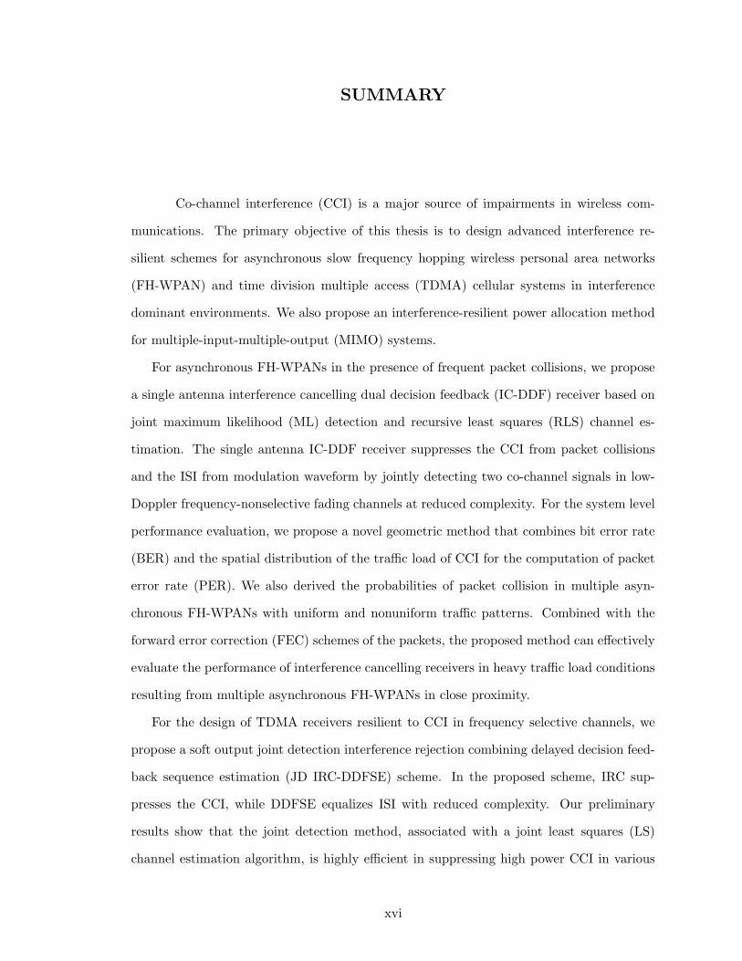
Co-channel interference (CCI) is a major source of impairments in wireless com-

munications. The primary objective of this thesis is to design advanced interference re-

silient schemes for asynchronous slow frequency hopping wireless personal area networks

(FH-WPAN) and time division multiple access (TDMA) cellular systems in interference

dominant environments. We also propose an interference-resilient power allocation method

for multiple-input-multiple-output (MIMO) systems.

For asynchronous FH-WPANs in the presence of frequent packet collisions, we propose

a single antenna interference cancelling dual decision feedback (IC-DDF) receiver based on

joint maximum likelihood (ML) detection and recursive least squares (RLS) channel es-

timation. The single antenna IC-DDF receiver suppresses the CCI from packet collisions

and the ISI from modulation waveform by jointly detecting two co-channel signals in low-

Doppler frequency-nonselective fading channels at reduced complexity. For the system level

performance evaluation, we propose a novel geometric method that combines bit error rate

(BER) and the spatial distribution of the traffic load of CCI for the computation of packet

error rate (PER). We also derived the probabilities of packet collision in multiple asyn-

chronous FH-WPANs with uniform and nonuniform traffic patterns. Combined with the

forward error correction (FEC) schemes of the packets, the proposed method can effectively

evaluate the performance of interference cancelling receivers in heavy traffic load conditions

resulting from multiple asynchronous FH-WPANs in close proximity.

For the design of TDMA receivers resilient to CCI in frequency selective channels, we

propose a soft output joint detection interference rejection combining delayed decision feed-

back sequence estimation (JD IRC-DDFSE) scheme. In the proposed scheme, IRC sup-

presses the CCI, while DDFSE equalizes ISI with reduced complexity. Our preliminary

results show that the joint detection method, associated with a joint least squares (LS)

channel estimation algorithm, is highly efficient in suppressing high power CCI in various

xvi

channel models. Also, the soft outputs are generated from IRC-DDFSE decision metric to

improve the performance of iterative or non-iterative type soft-input outer code decoders.

For the design of interference resilient power allocation scheme in MIMO systems, we

investigate an adaptive power allocation method using subset antenna transmission (SAT)

techniques. Motivated by the observation of capacity imbalance among the multiple parallel

sub-channels, the SAT method achieves high spectral efficiency by allocating power on a

selected transmit antenna subset. Increased transmit power per transmit antenna with

SAT scheme achieves larger spectral efficiency than all-antenna transmission method in the

presence of high power CCI. For 4×4 V-BLAST MIMO systems, the proposed scheme with

SAT showed analogous results. Adaptive modulation schemes combined with the proposed

method increase the capacity gains. From a feasibility viewpoint, the proposed method is a

practical solution to CCI-limited MIMO systems since it does not require the channel state

information (CSI) of CCI.

xvii

CHAPTER I

INTRODUCTION

During the last two decades, wireless communication has evolved from an optional con-

venience to an indispensable necessity in daily life. Advances in digital signal processing,

digital computing, and radio transmission technologies have facilitated the introduction of a

wide range of wireless communication services. Second generation wireless mobile commu-

nication systems such as GSM, IS-95, IS-136 and PDC provide people reliable narrowband

communication links mostly for voice and text traffics with high mobility, and high-speed

private- and public-access wireless local/personal area networks (WLAN/WPAN) such as

Wi-Fi and Bluetooth deliver broadband multimedia traffic with limited mobility. However,

increasing demands on high-capacity wireless multimedia services with sufficient mobility

have created challenging tasks to the designers of next generation wireless mobile commu-

nication systems.

Because of the randomness of the mobile propagation channels and limited radio spec-

trum, co-channel interference (CCI), fading and intersymbol interference (ISI) are major

impediments to high-capacity transmission in power- and bandwidth-limited wireless com-

munication systems. Fading is traditionally countermeasured by channel coding and inter-

leaving techniques as well as transmit/receive antenna diversity schemes. ISI from multi-

path reception can be combated by various linear/nonlinear type equalization techniques

employing symbol-by-symbol detection methods such as decision feedback equalizer (DFE)

or sequence-estimation methods such as maximum likelihood sequence estimation (MLSE).

In cellular networks, CCI is the interference from neighboring cells using the same radio

channels. As the frequency reuse factor decreases from seven to three, then to one, CCI

is unavoidable due to the channel reuse in adjacent cells. On the other hand, in ad-hoc

type wireless networks such as WLAN and WPAN, the signals transmitted from multiple

networks operating in close proximity behave as CCI to each other. Given perfect knowledge

1

of the channel coefficients of all co-channel signals, CCI is best handled by the joint MLSE

(J-MLSE) receiver, but J-MLSE is generally too complex. Less complex linear filter type

receivers suppress CCI by controlling the filter coefficients in the sense of maximizing the

signal-to-interference-plus-noise ratio (SINR).

In typical wireless mobile communication systems, CCI, ISI and fading often arise to-

gether. Hence, the receiver designs for mitigating these impairments in joint fashions are

quite common. In filter-based approaches, CCI is suppressed by a feedforward linear filter

while ISI is mitigated by a concatenated decision feedback filter [97]. For the receivers with

multiple antennas, diversity combining techniques broaden the freedom in interference mit-

igation receiver designs. Combined with MLSE or DFE type receivers, diversity combining

combat ISI and fading jointly. For the suppression of CCI in flat fading channels, an op-

timum linear minimum mean square error (MMSE) combining technique was suggested by

Winters [146]. Also, joint mitigation of CCI and ISI employing sequence estimation tech-

niques can be found in many references. Concatenation of MMSE filtering and MLSE has

been proposed by Bottomley et al. [27], and extended to an interference rejection combin-

ing MLSE (IRC-MLSE) receiver [28]. The complexity issue of MLSE structure in channels

with long channel impulse responses has been handled by employing less complex delayed

decision feedback sequence estimation (DDFSE) [84].

Multiuser detection (MUD) algorithms detect all co-channel signals unlike the filter-

based methods treating all co-channel signals, except the desired one, as interference. After

Van Etten [46] suggested a joint detection of co-channel signals by extending Forney’s

maximum-likelihood receiver [50], diverse MUD algorithms based on linear/nonlinear tech-

niques such as joint MLSE, decorrelator, linear MMSE, and parallel/successive interference

cancellation (PIC/SIC) have been proposed for practical code/time division multiple access

(CDMA/TDMA) receiver designs [29,39,40,118,140,143,148].

In multiple-input multiple-output (MIMO) systems, large spectral efficiency can be

achieved if the spatially multiplexed data streams, which manifest themselves as CCI to

each other, are properly separated [51]. Accordingly, CCI mitigation techniques developed

for single antenna systems have been applied in decoding of multi-channel data streams

2

in MIMO systems. In the Bell Labs layered space-time (BLAST) architectures, successive

decoding of spatially multiplexed data streams have been suggested by using zero-forcing

(ZF) or MMSE type linear receivers [52,147]. On the other hand, the spectral efficiency of a

MIMO system, which heavily depends on the optimality of the power allocation algorithm,

reduces in the presence of CCI [26]. For additive white Gaussian noise (AWGN) channels,

the power allocation based on a water-filling and equal-distribution algorithms are known

optimum to attain channel capacity when transmitters have channel state information (CSI)

or not, respectively [34,51]. However, in the presence of unknown high power CCI or noise,

eigenmode imbalance in channel matrices wastes the power allocated to the eigenmodes with

small eigenvalues when the CSI of CCI is not available [74]. Accordingly, antenna subset

selection techniques have attracted significant attention because of the benefit of reduced

cost in hardware implementation while improving error performance of linear/nonlinear

receivers and transmitters [57, 69,120].

1.1 Problem and Solution

The impairments from CCI and ISI have been major obstacles to reliable communication in

long-range cellular networks and in short-range wireless local- and personal-area networks.

Linear filtering, equalization, and diversity combining techniques have been traditional

means to combat the impairments in separate or joint fashions. Also, the interference-

cancelling techniques designed for decoding of multiple single-user signals have been ap-

plied in decoding of spatially multiplexed data streams in MIMO systems [52]. However,

the impairments from high-power CCI and ISI in time-varying channels still impose severe

constraints in the design of practical interference resilient receivers [26, 28, 156]. In the

following, some of problems encountered in the design of interference mitigation receivers

in the area of asynchronous FH-WPANs, TDMA cellular systems, and MIMO systems are

presented along with the proposed solutions.

3

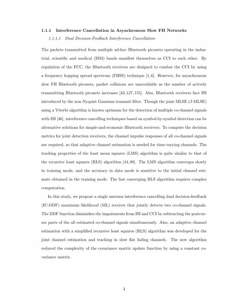
1.1.1 Interference Cancellation in Asynchronous Slow FH Networks

1.1.1.1 Dual Decision-Feedback Interference Cancellation

The packets transmitted from multiple ad-hoc Bluetooth piconets operating in the indus-

trial, scientific and medical (ISM) bands manifest themselves as CCI to each other. By

regulation of the FCC, the Bluetooth receivers are designed to combat the CCI by using

a frequency hopping spread spectrum (FHSS) technique [1, 6]. However, for asynchronous

slow FH Bluetooth piconets, packet collisions are unavoidable as the number of actively

transmitting Bluetooth piconets increases [43, 127, 155]. Also, Bluetooth receivers face ISI

introduced by the non-Nyquist Gaussian transmit filter. Though the joint MLSE (J-MLSE)

using a Viterbi algorithm is known optimum for the detection of multiple co-channel signals

with ISI [46], interference cancelling techniques based on symbol-by-symbol detection can be

alternative solutions for simple-and-economic Bluetooth receivers. To compute the decision

metrics for joint detection receivers, the channel impulse responses of all co-channel signals

are required, so that adaptive channel estimation is needed for time-varying channels. The

tracking properties of the least mean squares (LMS) algorithm is quite similar to that of

the recursive least squares (RLS) algorithm [44, 98]. The LMS algorithm converges slowly

in training mode, and the accuracy in data mode is sensitive to the initial channel esti-

mate obtained in the training mode. The fast converging RLS algorithm requires complex

computation.

In this study, we propose a single antenna interference cancelling dual decision-feedback

(IC-DDF) maximum likelihood (ML) receiver that jointly detects two co-channel signals.

The DDF function diminishes the impairments from ISI and CCI by subtracting the postcur-

sor parts of the all estimated co-channel signals simultaneously. Also, an adaptive channel

estimation with a simplified recursive least squares (RLS) algorithm was developed for the

joint channel estimation and tracking in slow flat fading channels. The new algorithm

reduced the complexity of the covariance matrix update function by using a constant co-

variance matrix.

4

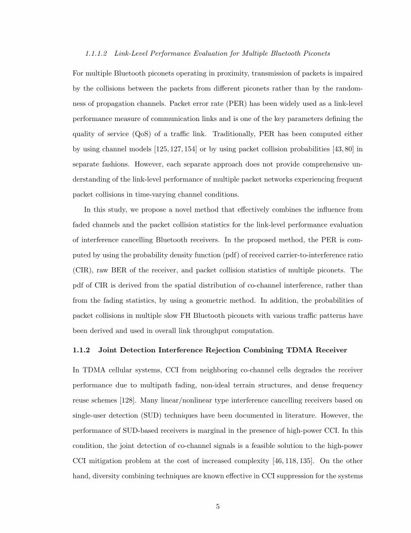
1.1.1.2 Link-Level Performance Evaluation for Multiple Bluetooth Piconets

For multiple Bluetooth piconets operating in proximity, transmission of packets is impaired

by the collisions between the packets from different piconets rather than by the random-

ness of propagation channels. Packet error rate (PER) has been widely used as a link-level

performance measure of communication links and is one of the key parameters defining the

quality of service (QoS) of a traffic link. Traditionally, PER has been computed either

by using channel models [125, 127, 154] or by using packet collision probabilities [43, 80] in

separate fashions. However, each separate approach does not provide comprehensive un-

derstanding of the link-level performance of multiple packet networks experiencing frequent

packet collisions in time-varying channel conditions.

In this study, we propose a novel method that effectively combines the influence from

faded channels and the packet collision statistics for the link-level performance evaluation

of interference cancelling Bluetooth receivers. In the proposed method, the PER is com-

puted by using the probability density function (pdf) of received carrier-to-interference ratio

(CIR), raw BER of the receiver, and packet collision statistics of multiple piconets. The

pdf of CIR is derived from the spatial distribution of co-channel interference, rather than

from the fading statistics, by using a geometric method. In addition, the probabilities of

packet collisions in multiple slow FH Bluetooth piconets with various traffic patterns have

been derived and used in overall link throughput computation.

1.1.2 Joint Detection Interference Rejection Combining TDMA Receiver

In TDMA cellular systems, CCI from neighboring co-channel cells degrades the receiver

performance due to multipath fading, non-ideal terrain structures, and dense frequency

reuse schemes [128]. Many linear/nonlinear type interference cancelling receivers based on

single-user detection (SUD) techniques have been documented in literature. However, the

performance of SUD-based receivers is marginal in the presence of high-power CCI. In this

condition, the joint detection of co-channel signals is a feasible solution to the high-power

CCI mitigation problem at the cost of increased complexity [46, 118, 135]. On the other

hand, diversity combining techniques are known effective in CCI suppression for the systems

5

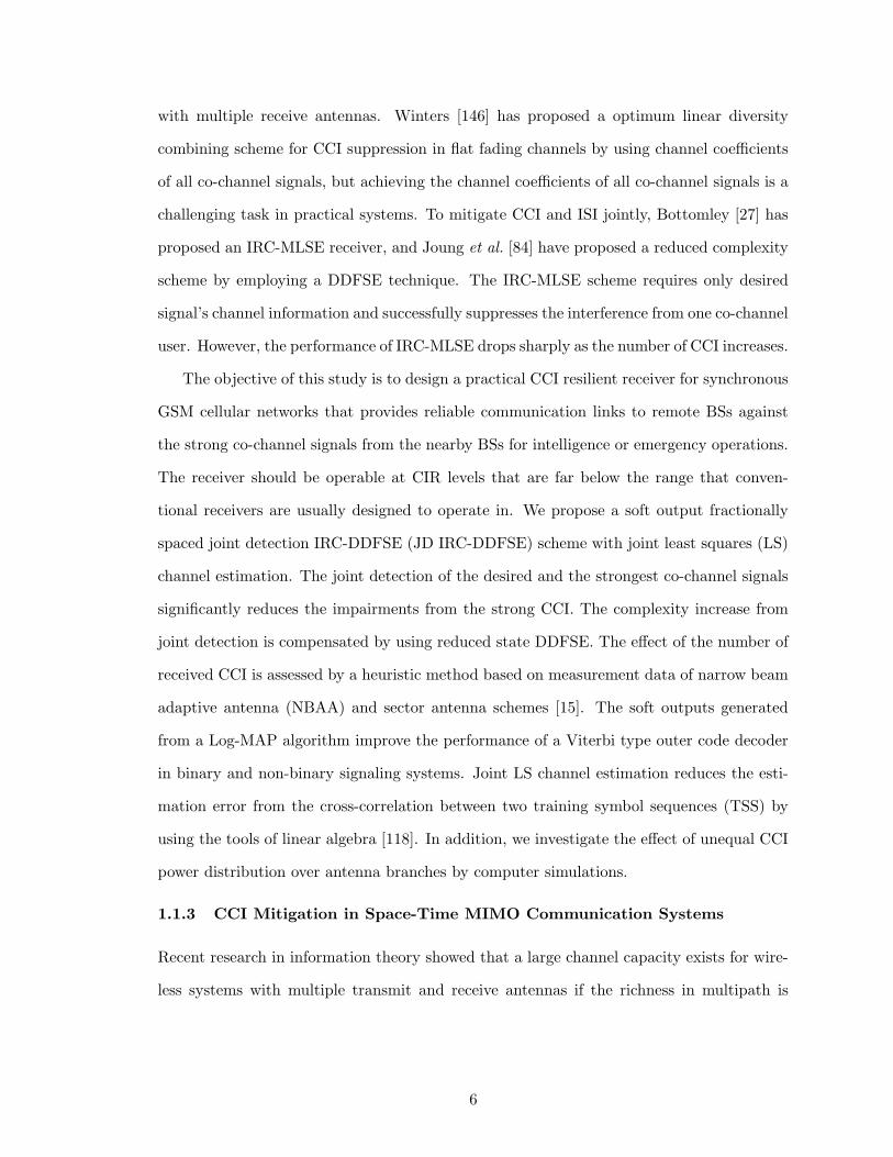
with multiple receive antennas. Winters [146] has proposed a optimum linear diversity

combining scheme for CCI suppression in flat fading channels by using channel coefficients

of all co-channel signals, but achieving the channel coefficients of all co-channel signals is a

challenging task in practical systems. To mitigate CCI and ISI jointly, Bottomley [27] has

proposed an IRC-MLSE receiver, and Joung et al. [84] have proposed a reduced complexity

scheme by employing a DDFSE technique. The IRC-MLSE scheme requires only desired

signal’s channel information and successfully suppresses the interference from one co-channel

user. However, the performance of IRC-MLSE drops sharply as the number of CCI increases.

The objective of this study is to design a practical CCI resilient receiver for synchronous

GSM cellular networks that provides reliable communication links to remote BSs against

the strong co-channel signals from the nearby BSs for intelligence or emergency operations.

The receiver should be operable at CIR levels that are far below the range that conven-

tional receivers are usually designed to operate in. We propose a soft output fractionally

spaced joint detection IRC-DDFSE (JD IRC-DDFSE) scheme with joint least squares (LS)

channel estimation. The joint detection of the desired and the strongest co-channel signals

significantly reduces the impairments from the strong CCI. The complexity increase from

joint detection is compensated by using reduced state DDFSE. The effect of the number of

received CCI is assessed by a heuristic method based on measurement data of narrow beam

adaptive antenna (NBAA) and sector antenna schemes [15]. The soft outputs generated

from a Log-MAP algorithm improve the performance of a Viterbi type outer code decoder

in binary and non-binary signaling systems. Joint LS channel estimation reduces the esti-

mation error from the cross-correlation between two training symbol sequences (TSS) by

using the tools of linear algebra [118]. In addition, we investigate the effect of unequal CCI

power distribution over antenna branches by computer simulations.

1.1.3 CCI Mitigation in Space-Time MIMO Communication Systems

Recent research in information theory showed that a large channel capacity exists for wire-

less systems with multiple transmit and receive antennas if the richness in multipath is

6

properly exploited [51]. The capacity of a MIMO system depends on the number of trans-

mit/receive antennas, the correlation between the channel coefficients of individual paths,

and the power allocation scheme over the transmit antennas [126,147]. For AWGN channels,

the power allocation based on a water-filling algorithm is known to attain capacity when the

transmitters have CSI [34]. Likewise, the equal power distribution is an alternative solution

if CSI is not available at the transmitter [51]. Unlike the Gaussian noise, however, CCI

is generally treated as colored noise having non-zero off-diagonal terms in its covariance

matrix. Hence, the power allocation must be optimized with an equivalent channel matrix

derived from the CSI of desired and interfering signals [48]. However, the estimation of

the CSI of interfering signals, which is an essential part of the equivalent channel matrix,

is a challenging task in many practical systems. Also, the equal power distribution is not

promising in the presence of high-power interference-plus-noise because of the elimination

of all but a few largest eigenvalues in such conditions [22,111]. To mitigate the capacity loss

from CCI, MIMO multiuser detection and adaptive power allocation by subspace tracking

were proposed [26, 64, 153]. But, they are impractical when the transmitter either has a

large number of antennas or does not have the CSI for all co-channel signals.

In this study, we investigate the effect of adaptive power allocation by using subset an-

tenna transmission (SAT) on the capacity of MIMO systems in the presence of co-channel

interference (CCI). In the SAT scheme, the transmit power is redistributed equally across a

selected subset of the transmit antennas. The subset is determined from a criteria obtained

from the CSI of the desired signal, while CSI of the CCI is not needed. The capacity gain

from the proposed method is evaluated by numerical methods. For comparison, the perfor-

mance of a space-time diversity coding (STDC) scheme in terms of interference mitigation

is also provided.

1.2 Thesis Outline

This thesis is organized as follows. Chapter 2 reviews a brief background information on

interference sources in wireless communications and interference mitigation techniques for

various system models. Chapter 3 presents interference cancellation in Bluetooth networks,

7

where a cost-effective single antenna joint detection interference cancelling receiver and an

associated system level performance evaluation scheme are proposed. Chapter 4 considers a

practical soft output joint detection IRC-DDFSE TDMA receiver that mitigates the effect

of a strong CCI signal. Computer simulations were carried out to evaluate the performance

of the proposed receiver design for various GSM channel models. Chapter 5 analyzes the

performance of the proposed subset antenna transmission method for MIMO systems in

the presence of high-power interference and noise. Comparisons are made between the SAT

scheme and the conventional all-antenna transmission scheme in information theoretic ca-

pacity and realistic capacity of vertical-BLAST (V-BLAST) systems. Chapter 6 summarizes

the results obtained in this thesis, and proposes some topics for further study.

8

CHAPTER II

BACKGROUND

2.1 Interference in Wireless Communications

2.1.1 Propagation Channels

In wireless mobile communications, the transmitted signal is subject to various impairments

caused by the transmission medium combined with the mobility of transmitters and/or

receivers. Path-loss is an attenuation of the signal strength with the distance between the

transmitter and the receiver antenna, and the frequency reuse technique in cellular systems

is based on the physical phenomena of path-loss. Unlike the transmission in free space,

transmission in practical channels, where propagation takes place in atmosphere and near

the ground, is affected by terrain contours. As the mobile moves, the slow variation in mean

envelope over a small region, shadowing, appears due to the variations in large-scale terrain

characteristics, such as hills, forests, and clumps of buildings. The variations resulting

from shadowing, are often described by a log-normal distribution with standard deviation

ranging from 4 to 13 dB [62, 128]. Power control techniques are often used to combat the

slow variation in mean received envelope due to the path-loss and shadowing.

Compared to the large-scale fading due to the shadowing, multipath fading, often called

fast fading, refers to the small-scale fast fluctuation of the received signal envelope resulting

from multipath reception and transmitter and/or receiver movement. Multipath fading

results in the constructive or destructive addition of arriving plane wave components, and

manifests itself as large variations in amplitude and phase of the composite received signal

in time [82]. When the channel exhibits a deep fade, fading causes a very low instantaneous

signal-to-noise ratio (SNR) or carrier-to-noise ratio (CNR). Diversity and coding techniques

are well known methods for combating multipath fading by reducing the probability that

the received signal is weak.

9

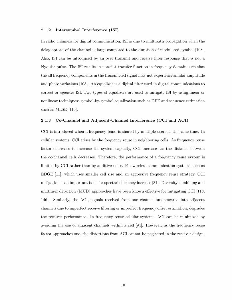
2.1.2 Intersymbol Interference (ISI)

In radio channels for digital communication, ISI is due to multipath propagation when the

delay spread of the channel is large compared to the duration of modulated symbol [108].

Also, ISI can be introduced by an over transmit and receive filter response that is not a

Nyquist pulse. The ISI results in non-flat transfer function in frequency domain such that

the all frequency components in the transmitted signal may not experience similar amplitude

and phase variations [108]. An equalizer is a digital filter used in digital communications to

correct or equalize ISI. Two types of equalizers are used to mitigate ISI by using linear or

nonlinear techniques: symbol-by-symbol equalization such as DFE and sequence estimation

such as MLSE [116].

2.1.3 Co-Channel and Adjacent-Channel Interference (CCI and ACI)

CCI is introduced when a frequency band is shared by multiple users at the same time. In

cellular systems, CCI arises by the frequency reuse in neighboring cells. As frequency reuse

factor decreases to increase the system capacity, CCI increases as the distance between

the co-channel cells decreases. Therefore, the performance of a frequency reuse system is

limited by CCI rather than by additive noise. For wireless communication systems such as

EDGE [11], which uses smaller cell size and an aggressive frequency reuse strategy, CCI

mitigation is an important issue for spectral efficiency increase [31]. Diversity combining and

multiuser detection (MUD) approaches have been known effective for mitigating CCI [118,

146]. Similarly, the ACI, signals received from one channel but smeared into adjacent

channels due to imperfect receive filtering or imperfect frequency offset estimation, degrades

the receiver performance. In frequency reuse cellular systems, ACI can be minimized by

avoiding the use of adjacent channels within a cell [94]. However, as the frequency reuse

factor approaches one, the distortions from ACI cannot be neglected in the receiver design.

10

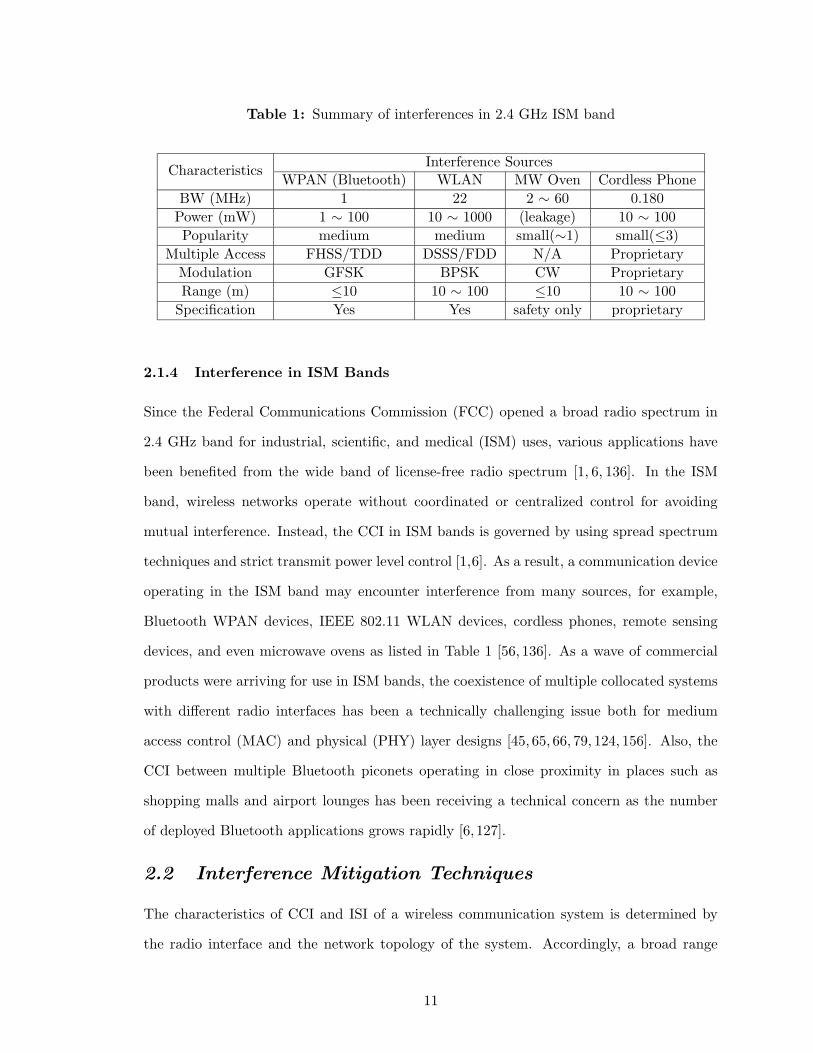
Table 1: Summary of interferences in 2.4 GHz ISM band

Interference SourcesCharacteristics

WPAN (Bluetooth) WLAN MW Oven Cordless Phone

BW (MHz) 1 22 2 ∼ 60 0.180

Power (mW) 1 ∼ 100 10 ∼ 1000 (leakage) 10 ∼ 100

Popularity medium medium small(∼1) small(≤3)

Multiple Access FHSS/TDD DSSS/FDD N/A Proprietary

Modulation GFSK BPSK CW Proprietary

Range (m) ≤10 10 ∼ 100 ≤10 10 ∼ 100

Specification Yes Yes safety only proprietary

2.1.4 Interference in ISM Bands

Since the Federal Communications Commission (FCC) opened a broad radio spectrum in

2.4 GHz band for industrial, scientific, and medical (ISM) uses, various applications have

been benefited from the wide band of license-free radio spectrum [1, 6, 136]. In the ISM

band, wireless networks operate without coordinated or centralized control for avoiding

mutual interference. Instead, the CCI in ISM bands is governed by using spread spectrum

techniques and strict transmit power level control [1,6]. As a result, a communication device

operating in the ISM band may encounter interference from many sources, for example,

Bluetooth WPAN devices, IEEE 802.11 WLAN devices, cordless phones, remote sensing

devices, and even microwave ovens as listed in Table 1 [56, 136]. As a wave of commercial

products were arriving for use in ISM bands, the coexistence of multiple collocated systems

with different radio interfaces has been a technically challenging issue both for medium

access control (MAC) and physical (PHY) layer designs [45, 65, 66, 79, 124, 156]. Also, the

CCI between multiple Bluetooth piconets operating in close proximity in places such as

shopping malls and airport lounges has been receiving a technical concern as the number

of deployed Bluetooth applications grows rapidly [6, 127].

2.2 Interference Mitigation Techniques

The characteristics of CCI and ISI of a wireless communication system is determined by

the radio interface and the network topology of the system. Accordingly, a broad range

11

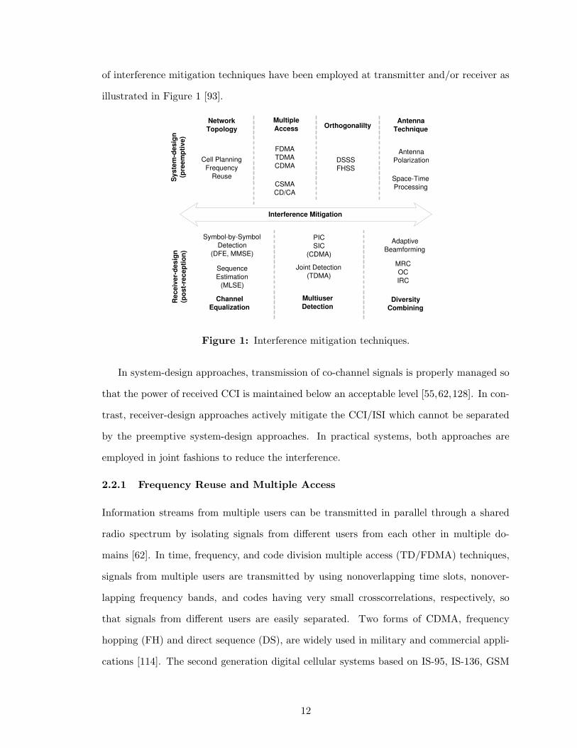
of interference mitigation techniques have been employed at transmitter and/or receiver as

illustrated in Figure 1 [93].

Antenna Technique

Multiple Access

Network Topology

FDMA TDMA CDMA

CSMA CD/CA

Cell Planning Frequency

Reuse

DSSS FHSS

Space-Time Processing

Channel Equalization

PIC SIC

(CDMA)

Antenna Polarization

Joint Detection (TDMA)

Diversity Combining

Symbol-by-Symbol Detection

(DFE, MMSE)

Sequence Estimation

(MLSE)

Multiuser Detection

MRC OC IRC

Adaptive Beamforming

Orthogonalilty

Sys

tem

-des

ign

(pre

empt

ive)

R

ecei

ver-

desi

gn

(pos

t-re

cept

ion)

Interference Mitigation

Figure 1: Interference mitigation techniques.

In system-design approaches, transmission of co-channel signals is properly managed so

that the power of received CCI is maintained below an acceptable level [55,62,128]. In con-

trast, receiver-design approaches actively mitigate the CCI/ISI which cannot be separated

by the preemptive system-design approaches. In practical systems, both approaches are

employed in joint fashions to reduce the interference.

2.2.1 Frequency Reuse and Multiple Access

Information streams from multiple users can be transmitted in parallel through a shared

radio spectrum by isolating signals from different users from each other in multiple do-

mains [62]. In time, frequency, and code division multiple access (TD/FDMA) techniques,

signals from multiple users are transmitted by using nonoverlapping time slots, nonover-

lapping frequency bands, and codes having very small crosscorrelations, respectively, so

that signals from different users are easily separated. Two forms of CDMA, frequency

hopping (FH) and direct sequence (DS), are widely used in military and commercial appli-

cations [114]. The second generation digital cellular systems based on IS-95, IS-136, GSM

12

and PDC standards are designed using a combination of the three multiple access techniques

to accommodate more channels [55].

Frequency reuse is an example of space division multiple access (SDMA) techniques that

separates CCI in cellular systems by utilizing path loss phenomena and radio spectrum par-

titioning [55,94]. In a frequency reuse scheme, clustered radio channels are reused in distant

co-channel cells in repeating patterns. The transmit power is properly controlled to keep

the amount of CCI at a tolerable level. However, the received CIR at a receiver is not guar-

anteed statistically because of the dynamic nature of the fading channels especially in high

capacity wireless systems where more aggressive frequency reuse schemes are employed [11].

Wireless packet networks (WLAN and WPAN) based on IEEE802.11 and Bluetooth

standards provide complementary wireless solutions for low-mobility broadband multimedia

traffic in the unlicensed ISM band [1, 6, 10]. The WLANs and WPANs operate in two

different network topologies: access-point and ad-hoc network. Without any centralized

multiple access control among collocated networks, independent multiple access control

(MAC) in each network such as carrier sensing multiple access with collision avoidance

(CSMA/CA) cannot avoid the collision between packets from different networks. Therefore,

CCI from packet collisions can only be mitigated by using direct sequence or frequency

hopping spread spectrum techniques at physical (PHY) layer signal processing.

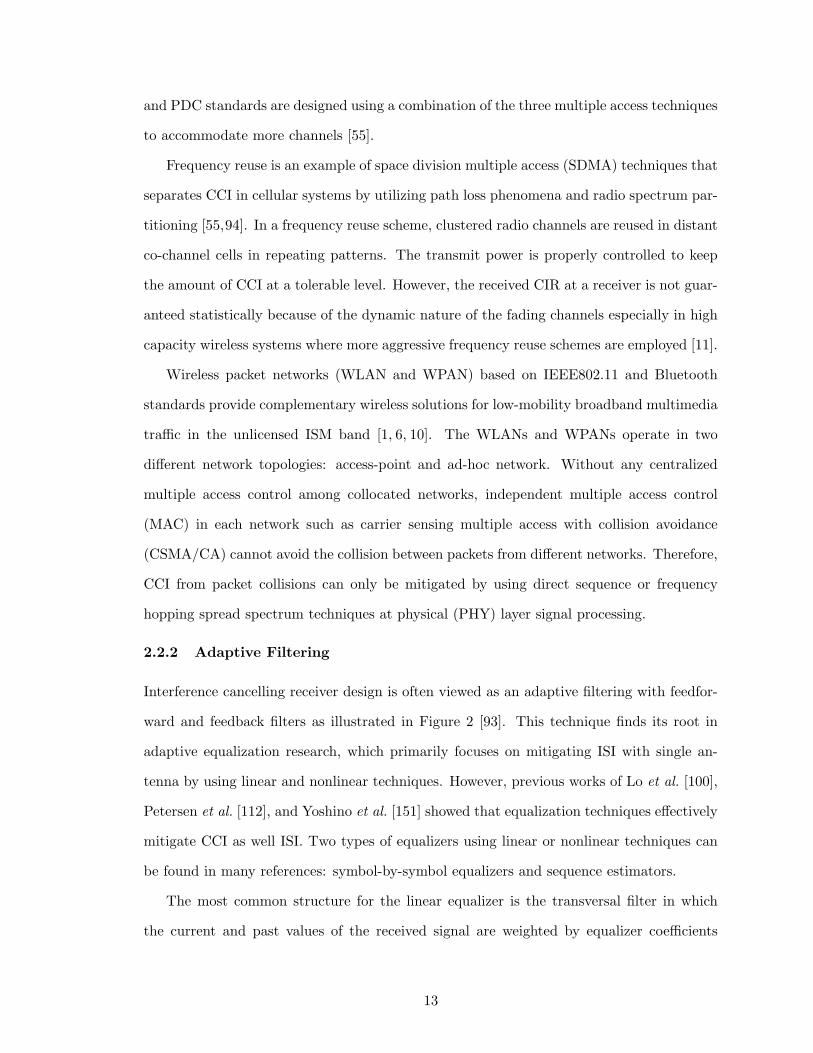
2.2.2 Adaptive Filtering

Interference cancelling receiver design is often viewed as an adaptive filtering with feedfor-

ward and feedback filters as illustrated in Figure 2 [93]. This technique finds its root in

adaptive equalization research, which primarily focuses on mitigating ISI with single an-

tenna by using linear and nonlinear techniques. However, previous works of Lo et al. [100],

Petersen et al. [112], and Yoshino et al. [151] showed that equalization techniques effectively

mitigate CCI as well ISI. Two types of equalizers using linear or nonlinear techniques can

be found in many references: symbol-by-symbol equalizers and sequence estimators.

The most common structure for the linear equalizer is the transversal filter in which

the current and past values of the received signal are weighted by equalizer coefficients

13

Adaptive Algorithm

Demodulator or Detector Adaptive Filter

Desired Signal or

Known Property

Estimate of Original Signal

Passband or

Baseband signal

Figure 2: An adaptive filter model for interference mitigation.

and summed to produce the output for symbol-by-symbol decisions on the received symbol

sequence. The equalizer coefficients are adjusted to minimize some error criterion. The

equalizer that forces ISI to zero is called zero-forcing (ZF) equalizer. The MMSE equalizer

outperforms the ZF equalizer in performance and convergence properties by mitigating the

noise enhancement [115, 116]. Nonlinear decision feedback equalizer (DFE) combined with

a linear feedforward filter has been proposed to reduce the effect of noise enhancement

from precursor and postcursor ISI. Lo et al. [100] showed that a directly adapted RLS DFE

equalizer outperforms an MMSE equalizer, which employs estimates of channel impulse

response and the autocorrelation of interference-plus-noise in frequency selective channels

in the presence of CCI [100]. One drawback of the DFE type receivers is error propagation

when the desired signal is in a deep fade, or when the received CIR is low. Uesugi et

al. [135] also proposed a DFE type single/double feedback interference cancelling (SF/DF-

IC) receiver to mitigate CCI by subtracting the ISI components of the estimated co-channel

signals.

The optimum maximum-likelihood sequence estimation (MLSE) receiver for signals cor-

rupted with ISI and AWGN was proposed by Forney [50]. MLSE uses a whitened-matched

filter (WMF) followed by a Virerbi decoder to combine equalization and decoding. An

MLSE type receiver requires the channel information for sequence estimation, and its com-

plexity increases exponentially with the length of the channel and the size of the signal

constellation. For tracking rapidly time-varying channels, adaptive algorithms such as the

LMS and the RLS algorithms are usually employed [135,151]. The suboptimum sequence es-

timation techniques were investigated for solutions with reduced complexities. Duel-Hallen

14

Table 2: Weight functions of diversity combining techniques with CCI

Weight Notes

EGC W = [1, . . . , 1] Co-phased and equally weighted

MRC W = [g∗1d, . . . , g∗Nd] = g∗

d ML with CSI

OC W = αR−1g∗d where R−1 = σ2I + E[g∗

i gTi ] Optimal in sense of Max. SINR

IRC metric = arg min{exp(−g∗i R

−1gTi )} MLSE from impairment vector

and Heegard proposed a delayed decision-feedback sequence estimator (DDFSE) [41]. This

algorithm provides tradeoffs between complexity and performance by using a truncated

state trellis and decision-feedback to compute branch metric. A reduced-state sequence es-

timation (RSSE) was proposed by Eyuboglu et al. [47] by using the idea of set-partitioning

algorithm initially proposed by Ungerboeck [137].

2.2.3 Spatio-Temporal Interference Mitigation

Faded signal reception results in a large penalty in SNR when the receiver has only one set

of received signals from a single antenna. For example, a DFE type receiver with a single

antenna experiences error propagation during the signal reception in a deep fade. The use

of multiple antennas at receiver creates multiple-input multiple-output (MIMO) channels

in CCI mitigation [128], and the existing CCI mitigation techniques for multiple-input

single-output (MISO) channels can be extended to spatio-temporal interference mitigation

techniques by using diversity combing techniques. One advantage of the spatio-temporal

approach is a joint suppression-and-equalization of CCI and ISI [27,84,97].

2.2.3.1 Diversity Combining for CCI Suppression

Figure 3 illustrates an architecture of the 1×N diversity combining receiver with channel

vectors gd = [g1d, . . . , gNd] and gi = [g1i, . . . , gNi] of the desired and interfering signals,

respectively. Weight functions of four different diversity combining techniques are sum-

marized in Table 2. Aalo et al. [12], Hafeez et al. [72], Shah et al. [122], and Rao et

al. [119]have analyzed the performance of optimum combining (OC) and MRC techniques

with non-Gaussian CCI in flat fading channels in terms of outage probability. Suzuki [130]

15

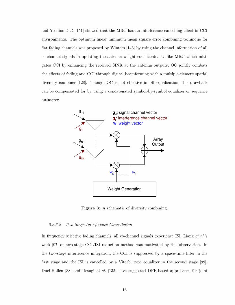
and Yoshinoet al. [151] showed that the MRC has an interference cancelling effect in CCI

environments. The optimum linear minimum mean square error combining technique for

flat fading channels was proposed by Winters [146] by using the channel information of all

co-channel signals in updating the antenna weight coefficients. Unlike MRC which miti-

gates CCI by enhancing the received SINR at the antenna outputs, OC jointly combats

the effects of fading and CCI through digital beamforming with a multiple-element spatial

diversity combiner [128]. Though OC is not effective in ISI equalization, this drawback

can be compensated for by using a concatenated symbol-by-symbol equalizer or sequence

estimator.

Array Output

g 1d

g Nd

w 1 w N

g 1i

g Ni

Weight Generation

g d : signal channel vector

w : weight vector g i : interference channel vector

Figure 3: A schematic of diversity combining.

2.2.3.2 Two-Stage Interference Cancellation

In frequency selective fading channels, all co-channel signals experience ISI. Liang et al.’s

work [97] on two-stage CCI/ISI reduction method was motivated by this observation. In

the two-stage interference mitigation, the CCI is suppressed by a space-time filter in the

first stage and the ISI is cancelled by a Viterbi type equalizer in the second stage [99].

Duel-Hallen [38] and Uesugi et al. [135] have suggested DFE-based approaches for joint

16

suppression-and-equalization in MIMO channels. Li et al. [96] also proposed CCI/ISI miti-

gation for IS-136 TDMA systems by using MMSE spatial-temporal DFE and linear equalizer

(LE).

With sequence estimation equalizers, joint MLSE (J-MLSE) is the maximum-likelihood

solution to the signal detection in the ISI channels with CCI [46]. Besides its computational

complexity, J-MLSE requires channel coefficients of all co-channel signals, which is mostly

infeasible in practical systems. As an alternative solution to J-MLSE, an interference re-

jection combining MLSE (IRC-MLSE) receiver, which only requires channel information of

the desired user, was proposed by Bottomley et al. [27]. The IRC-MLSE receiver structure

exploits the cross-correlation of the signal impairments of interference-plus-noise across the

antenna arrays and combines diversity branches in the metric of the MLSE receiver. The

IRC-MLSE technique has been considered a practical solution in many interference-resilient

TDMA receiver designs [59,86,117].

Joung et al. [84] suggested a fractionally-spaced reduced complexity IRC-DDFSE re-

ceiver by employing the DDFSE technique initially proposed by Duel-Hallen [41]. The

IRC-DDFSE receiver uses a T/2-spaced noise whitening filter depending only on the trans-

mit pulse as suggested by Hamied and Stuber [73]. This receiver structure not only gives an

advantage of immunity to symbol timing errors but also requires no ideal bandpass filter. In

addition, generation of soft outputs from diversity combining metrics and their use in joint

detection and channel estimation have been suggested [18, 152]. An iterative soft output

decoding technique was also proposed for multiuser detection in TDMA systems [138].

For diversity combining receivers, the received CIRs at antenna branches are generally

assumed equal. However, this assumption is not always applicable, especially in diver-

sity combining with directional antennas. Mallik et al. [103] showed that the imbalance of

Gaussian noise across antenna branches degrades the performance of equal gain combining

(EGC) in correlated Rayleigh faded channels, and Lin [99] showed that optimal and selec-

tive combining receivers with linear/nonlinear equalizers achieve minimum BER when all

antenna branches have equal received SNRs.

17

2.2.3.3 Beamforming and Transmit Diversity

Beamforming and transmit diversity are two complementary techniques for using multiple

antennas in wireless communication systems. Beamforming achieves an array gain by lin-

early combining tap gains of an antenna array in highly correlated channels while transmit

diversity obtains a diversity gain by exploiting the independence among channels [53]. In

highly correlated line-of-sight (LOS) indoor channels, beamforming techniques provide CCI-

mitigation through spatial filtering [125]. The spatial filtering of CCI is achieved either by

shaping beams to have nulls in the directions of co-channel signals or by forming beams to

have a large gain in the direction of the desired signal [142]. For this reason, beamforming

requires estimation of the direction of arrival (DoA) of the desired or interfering signals.

Several variations of beamforming have been proposed: fixed, switched, and adaptive

beamforming. In fixed beamforming (FB) networks, an antenna array forms narrow multiple

beams in pre-selected directions for low-mobility users and suppresses the interference from

outside of the beamwidth. The multichannel multipoint distribution service (MMDS) for

broadband wireless access (BWA) is one example of FB networks [9, 123]. The switched

beamforming (SB) technique uses a switch to select the best beam to receive a particular

signal in FB networks. As the realizations of the space division multiple access (SDMA)

technique, the fixed and switched beamforming have been applied to existing TDMA cellular

networks [72, 81, 104]. In cellular systems, adaptive control of antenna array is required to

track the time-varying distribution of mobile users. Anderson et al. [15] has suggested an

adaptive antenna system for GSM and TDMA systems by using an adaptive beamforming

(AB) technique in downlink and an interference rejection combining technique in uplink.

The LMS or RLS algorithms are used in updating of the spatial characteristics of the AB

array.

Unlike the beamforming technique which changes the radiation pattern of an antenna

array to achieve array gains and CCI-mitigation by controlling the weights of array elements

in radio frequency (RF) level, the diversity gain of the transmit diversity (TD) is achieved by

combining the signals in baseband or intermediate frequency (IF) level [63]. As a result, TD

allows a lot of freedom in transmitter/receiver designs by combining coding and space-time

18

diversity techniques [37]. Space-time encoding techniques employed in transmitter helps

the separation of transmitted signals at the receiver by using the orthogonality between

space-time code matrices. In other words, CCI mitigation in transmit diversity is achieved

by using the space-time coding as well as the antenna diversity. Another advantage of

the transmit diversity scheme is the simplified receiver structure without loosing diversity

gains. Li et al. [95] suggested a simplified CCI/ISI mitigation receiver design based on a

transmit diversity scheme, and Tarokh and Jafarkhani [131] proposed a simplified differential

detection scheme which requires no channel information at transmitter and receiver by using

a differential coding across transmit antennas.

The third generation (3G) wireless communication systems W-CDMA [8] and cdma2000 [7]

have considered time diversity techniques as their key contributing technologies. Orthogo-

nal TD (OTD) [7] is an open loop method in which coded interleaved symbols are split into

even and odd symbol streams and transmitted using two different Walsh codes. Space-time

transmit diversity (STTD) [8] and space-time spreading (STS) [7] techniques use Wlash

codes and transmit diversity techniques which are very similar to the one proposed by

Alamouti [14]. Closed loop techniques are adaptive in nature. Switched TD (STD) was

adopted by cdma2000 as an extension of the open loop technique, time-switched time diver-

sity (TSTD). The mobile station (MS) uses the average received power from the common

pilots from each antenna, and makes a decision from which antenna it would like the BS to

transmit. W-CDMA adopted a more aggressive transmit adaptive array (TXAA) method

which optimizes the transmitter weight to deliver maximum power to the MS. The MS

computes the weights and transmits to the BS. The precision, feedback error and feedback

delay are the technical issues requiring further research.

2.2.4 Multiuser Detection

Distinguished from single-user detection techniques, which treats signals from co-channel

users as interference, multi-user detection (MUD) detects all co-channel signals simultane-

ously. Since MUD techniques not only increase the system capacity but also improve the

quality of an individual communication link by eliminating CCI from multi-users [16], MUD

19

has been an important technology in interference-limited communication systems such as

GSM, IS-54/IS-136, and IS-95 regardless of the multiple access schemes [77].

After the concept of MUD based on the J-MLSE technique was introduced by Van Et-

ten [46] in 1976, a number of optimum and suboptimum MUD receiver designs have been

suggested mostly for CDMA cellular systems. In CDMA cellular systems based on DSSS

techniques, all co-channel users behave as wideband interference (WBI) to each other be-

cause of the low cross-correlation spreading codes [5, 91]. However, the near-far problem

and imperfect power-control limit the system capacity of the existing single-user detection

systems. The optimum multiuser detector for asynchronous CDMA systems was proposed

by Verdu [143]. However, the complexity of the optimum detector, which increases propor-

tional to O(Mk) where M is the alphabet size and k is the number of users, has prompted

the research on reduced-complexity suboptimum receivers. These suboptimum receiver de-

signs include the decorrelator detectors [101, 102], linear MMSE detectors [148], nonlinear

decision feedback detectors [39, 40], and multi-stage detectors with successive and parallel

interference cancellations (SIC/PIC) [29,140,141]. SIC is known to outperform PIC in real-

istic conditions where the users have unequal received power levels [109]. Imperfect channel

estimation and power control are the major sources of performance loss in SIC. An unequal

weighting technique and a binary iterative feedback algorithm have been suggested by An-

drew et al. [17] and Agrawal et al. [13] , respectively, to improve the channel estimation and

power control efficiency in SIC.

Similarly, a joint interference cancelling receiver based on DFE technique was suggested

by Uesugi et al. [135] for the Japanese TDMA celluar system, and Hafeez et al. [71], Hoeher

et al. [76], and Ranta et al. [118] proposed practical MUD receives for TDMA-based GSM,

EDGE, and IS-54/IS-136 systems, respectively, by using joint sequence estimation tech-

niques based on J-MLSE. To reduce the state of the J-MLSE method, reduced-state joint

detection algorithms based on the DDFSE technique have been suggested [76, 88]. Also,

the single-antenna interference cancellation (SAIC) techniques for TDMA cellular systems

have been considered as practical solutions for capacity increase without modifying exist-

ing infrastructures [20]. The results from computer simulations and field trials witnessed

20

the feasibility of the SAIC techniques based on joint-demodulation and blind interference

cancellation techniques in existing TDMA networks [32,113].

2.3 Packet-Level Performance in Wireless Communication

In present and future wireless digital communication systems such as GSM/EDGE, 3G

cellular systems, Wi-Fi, and Bluetooth, the transmission of multimedia traffic is organized

and transmitted in packets [1, 4, 6, 11]. The transmission of a packet is often protected

by a forward error correction (FEC) scheme. When a packet arrives with more bit errors

than the FEC scheme can restore, a packet error occurs and the erroneous packet generally

needs to be retransmitted. Also, FER is one of the key parameters defining the quality-

of-service (QoS) of a communication network [49]. As a result, PER is widely accepted

as a performance measure of wired and wireless communication networks regardless of the

nature of the propagation channels.

2.3.1 AWGN Channels

In AWGN channels, the transmission of each uncoded bit can be considered an independent

and identically distributed (i.i.d) process. With this assumption, the probability of packet

error Ppkt(e) can be represented in a binomial distribution with the probability of bit error

Pbit(e) as

Ppkt(e) = 1−Nmax∑

i=0

(

L

i

)

(Pbit(e))i(1− Pbit(e))

L−i (1)

where L, Ne, and Nmax represent the packet length, the number of bit errors during packet

transmission, and the number of maximum bit errors which can be corrected with a given

FEC scheme, respectively.

2.3.2 Time-Varying Fading Channels

In mobile communications, transmitted signals experience time-varying fading channels due

to the multipath reception and mobility of receivers and/or transmitters. For fast fading

channels where the received signal power changes rapidly bit-by-bit, transmission of each bit

and corresponding bit error probability can be considered an i.i.d process [154]. The systems

employing ideal interleavers employ the same model even in slow fading channels [25].

21

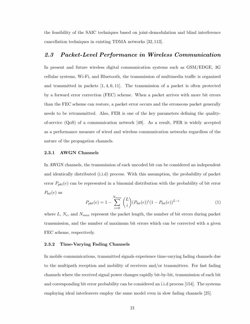
For slow fading channels where fades maintain for more than a one-bit baud interval

but change during the block transmission, the signal transmission at every baud interval

cannot be considered as an i.i.d process unless the transmitted bits are ideally interleaved.

In these channel conditions, a packet error is determined by the fade duration and the FEC

function of the packet [25,92]. In a packet error model proposed by Lai and Mandayam [92],

a packet is considered lost if the sum of the fade durations τf =∑

i τbi is greater than a

given threshold τth, where τth = Tb×Nmax is the baud duration multiplied by the maximum

number of bit errors allowed with a given FEC scheme. In Rayleigh faded channels, the

probability of packet error is given as [92]

Pτf(τf > τth) =

2

uI1(

2

πu2) exp(− 2

πu2) (2)

where I1(z) is a Bessel function of imaginary argument and u is the normalized fade duration

u = τth/τth with the mean duration of τth. Figure 4 illustrates the effect of the fade duration

during a packet reception.

packet

r(t)

t

PSfrag replacements

γth

τb1 τb2

Figure 4: Packet reception in slow faded channels.

The block fading channel model, in which the channel state is assumed to change at every

block interval and to remain unchanged during the block transmission, is widely accepted

for packet error modelling in quasi-static channels [125]. Zorzi et al. [154] has suggested a

packet success/failure model for noninterleaved packets in block fading channels by using a

22

first-order Markov process. In fast fading channels, the Markov process degenerates into an

i.i.d process. In a simplified threshold-type PER computation model suggested by Souissi

and Meihofer [127], a packet is considered erroneous if its received SINR γrx is smaller than

a given threshold γth as

Ppkt(e) = P (γrx < γth). (3)

2.3.3 Uncoordinated Wireless Packet Networks

For multiple asynchronous wireless packet networks operating in close proximity, the prob-

ability of packet error can be defined as

Ppkt(e) = Ppkt(e|c)P (c) + Ppkt(e|nc)(1− P (c)) (4)

where Ppkt(e|c) and Ppkt(e|nc) are the conditional probabilities of packet error with and

without collision, respectively, with a given probability of collision P (c). In short-range

low-mobility wireless communication systems such as WLAN and Bluetooth WPAN, trans-

mitted packets face negligible distortion from low-Doppler high-visibility propagation chan-

nels, and the probability of packet error defined in (4) is dominated by the first term of the

right side of the equation [156].

In a simple packet collision model used by Howitt [80] for a Bluetooth interference

modelling, a packet collision takes place if more than two packets share a radio channel

simultaneously regardless of their received power levels. More complicated models proposed

by Golmie et al. [66], Kamerman [85], and Van Dyck [139] have considered the capture effect,

path loss, and the network topologies in combined ways in the decision of a packet collision.

To compute the Ppkt(e|c) in asynchronous packet collisions, Shellhammern [124] suggested

the use of the number of the bits involved in the collision and the FEC scheme of the packet.

Previous studies on coexistence of WLAN and Bluetooth piconets in the ISM band have

focused on the packet collision and associated link throughput in ad-hoc and access-point

network topology models [66, 85, 124, 139, 156]. El-Hoiydi [43] simplified the computation

of the probability of packet collisions between synchronous (SCO) and asynchronous (ACL)

Bluetooth piconets by introducing the duty factors of the traffic links. Many analytical

23

models on the mutual interference among multiple collocated piconets carrying SCO/ACL

traffic have been documented in literature [33,80,127,155].

2.4 CCI and Channel Capacity in MIMO Systems

2.4.1 Channel State Information (CSI) and Power Allocation

In wireless communications, achieving a higher data rate is a challenging task for power

and bandwidth limited systems. Recent researches in information theory showed that the

capacity of a MIMO system depends on the number of transmit/receive antennas and the

correlation between the channel coefficients of individual paths, and the capacity can be

achieved by using a proper power allocation scheme over the transmit antennas [51,147]. The

power allocation by a water-filling algorithm is known capacity-optimum when transmitters

know CSI, while the equal power distribution is an alternative solution if CSI is not available

at the transmitters [52, 106]. In a system having a single-user link on M transmit and N

receive antennas (M ≤ N), the mutual information of the MIMO channels is [34, 134]

I = log2 det(HHHΦ + IM ) (5)

where H, Φ = E{ssH}, and I are the channel matrix, the covariance matrix of the trans-

mitted signals s, and an identity matrix, respectively. The random matrix W = HHH has a

Wishart distribution, and the distribution of the eigenvalues and condition numbers of W is

well explained in [42]. The parallel eigenmodes, which are represented with eigenvalues and

corresponding allocated powers, can be modelled as multiple pipes with different diameters

and corresponding amount of liquids running through them. When the CSI is available at

transmitters, the channel capacity is achieved with water-filling method by choosing Φ to

maximize the mutual information with the power constraints tr(Φ) ≤ PT [34].

In contrast, if no CSI is available at transmitters, Foschini [52] showed that the equal

power allocation scheme achieves the capacity. Considering the capacity achieved by water-

filling method, the equal-power allocation method is suboptimum, but this is the only

practical solution available if no CSI is available at the transmitters.

24

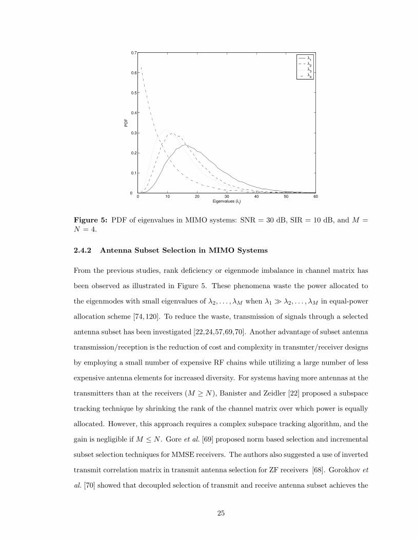
0 10 20 30 40 50 600

0.1

0.2

0.3

0.4

0.5

0.6

0.7

Eigenvalues (λi)

PD

F

λ1

λ2

λ3

λ4

Figure 5: PDF of eigenvalues in MIMO systems: SNR = 30 dB, SIR = 10 dB, and M =N = 4.

2.4.2 Antenna Subset Selection in MIMO Systems

From the previous studies, rank deficiency or eigenmode imbalance in channel matrix has

been observed as illustrated in Figure 5. These phenomena waste the power allocated to

the eigenmodes with small eigenvalues of λ2, . . . , λM when λ1 � λ2, . . . , λM in equal-power

allocation scheme [74,120]. To reduce the waste, transmission of signals through a selected

antenna subset has been investigated [22,24,57,69,70]. Another advantage of subset antenna

transmission/reception is the reduction of cost and complexity in transmter/receiver designs

by employing a small number of expensive RF chains while utilizing a large number of less

expensive antenna elements for increased diversity. For systems having more antennas at the

transmitters than at the receivers (M ≥ N), Banister and Zeidler [22] proposed a subspace

tracking technique by shrinking the rank of the channel matrix over which power is equally

allocated. However, this approach requires a complex subspace tracking algorithm, and the

gain is negligible if M ≤ N . Gore et al. [69] proposed norm based selection and incremental

subset selection techniques for MMSE receivers. The authors also suggested a use of inverted

transmit correlation matrix in transmit antenna selection for ZF receivers [68]. Gorokhov et

al. [70] showed that decoupled selection of transmit and receive antenna subset achieves the

25

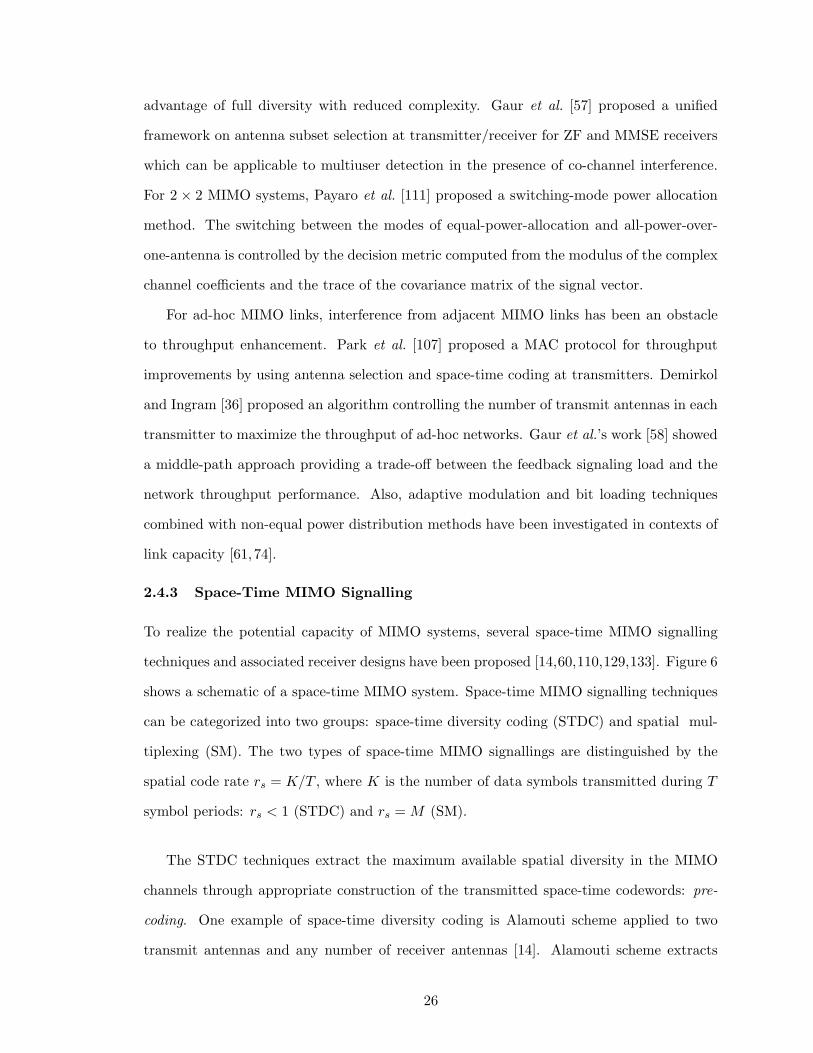
advantage of full diversity with reduced complexity. Gaur et al. [57] proposed a unified

framework on antenna subset selection at transmitter/receiver for ZF and MMSE receivers

which can be applicable to multiuser detection in the presence of co-channel interference.

For 2 × 2 MIMO systems, Payaro et al. [111] proposed a switching-mode power allocation

method. The switching between the modes of equal-power-allocation and all-power-over-

one-antenna is controlled by the decision metric computed from the modulus of the complex

channel coefficients and the trace of the covariance matrix of the signal vector.

For ad-hoc MIMO links, interference from adjacent MIMO links has been an obstacle

to throughput enhancement. Park et al. [107] proposed a MAC protocol for throughput

improvements by using antenna selection and space-time coding at transmitters. Demirkol

and Ingram [36] proposed an algorithm controlling the number of transmit antennas in each

transmitter to maximize the throughput of ad-hoc networks. Gaur et al.’s work [58] showed

a middle-path approach providing a trade-off between the feedback signaling load and the

network throughput performance. Also, adaptive modulation and bit loading techniques

combined with non-equal power distribution methods have been investigated in contexts of

link capacity [61,74].

2.4.3 Space-Time MIMO Signalling

To realize the potential capacity of MIMO systems, several space-time MIMO signalling

techniques and associated receiver designs have been proposed [14,60,110,129,133]. Figure 6

shows a schematic of a space-time MIMO system. Space-time MIMO signalling techniques

can be categorized into two groups: space-time diversity coding (STDC) and spatial mul-

tiplexing (SM). The two types of space-time MIMO signallings are distinguished by the

spatial code rate rs = K/T , where K is the number of data symbols transmitted during T

symbol periods: rs < 1 (STDC) and rs = M (SM).

The STDC techniques extract the maximum available spatial diversity in the MIMO

channels through appropriate construction of the transmitted space-time codewords: pre-

coding. One example of space-time diversity coding is Alamouti scheme applied to two

transmit antennas and any number of receiver antennas [14]. Alamouti scheme extracts

26

Transmitter

Space-Time Encoder

Information Stream

Space-Time Decoder

H

Receiver

Figure 6: A schematic of a space-time MIMO system model.

2Nth-order diversity gain with N receive antennas and can be extended to channels with

more than two transmit antennas through the orthogonal space-time block coding (OSTBC)

with low decoding complexity [132]. However, STDC signalling suffers capacity losses be-

cause of the small spatial code rate (rs < 1). Another example of space-time diversity

coding is the delay diversity which converts spatial diversity into frequency diversity by

transmitting the data symbols from the first antenna and a delayed replica of that from the

the second antenna [121]. The effective channel impulse response seen by the data symbols

is a symbol spaced two-path SISO channel with independent fading paths and equal average

path energy.

In spatial multiplexing, instead of maximizing the spatial diversity, the transmission

rate is maximized by sending M independent data symbols per symbol period from M

transmit antennas. By doing so, spatial multiplexing achieves a large spatial code rate

rs = M . For the transmission of M -symbol information streams, horizontal, vertical and

diagonal encoding (HE, V E, and DE) schemes are employed by using different spatial

multiplexing schemes [110].

2.4.4 Receiver Structures for Space-Time MIMO Systems

In space-time diversity coded systems, the orthogonality between the codes decouples the

vector detection problem into scalar detections [132]. Hence, zero-forcing (ZF), minimum-

mean square error estimation (MMSE), and ML sequence estimation (MLSE) type receivers

27

can be directly applied [110]. For the space-time trellis coded (STTC) systems, a Viterbi-

type sequence estimator should be used [133].

In spatially multiplexed systems, the receiver design faces the problem of mutual in-

terference between spatially multiplex information streams. Accordingly, there exists an

analogy between multiuser detection (MUD) and the decoding of spatially multiplexed sys-

tems in terms of the complexity-performance tradeoff. The ML receiver performs vector

decoding and is optimal in the sense of the error probability. A drawback of the ML type

receiver design is the decoding complexity, which grows exponentially with the alphabet size

and number of transmit antennas [144]. The complexity of ML decoding can be reduced by

employing linear receiver front-ends [23]. One simple realization of the linear receivers is

the ZF receiver which converts the joint decoding problem into M single stream decoding

problems. The noise enhancement in ZF receivers can be reduced in MMSE type receivers

by including the noise term in the front-end weight function. The MMSE receiver ap-

proaches the matched-filter receiver and the ZF receiver at low-SNR and high-SNR regions,

respectively [110].

The nonlinear BLAST type MIMO systems are based on the idea of successive can-

cellation in MIMO system where each individual data stream is successively decoded and

stripped away from the received data set for the reduced-interference decoding of the re-

maining data streams [51, 147]. For diagonally encoded systems (D-BLAST), the order of

successive decoding is determined by the transmission structure while the received SINR

determines the decoding order in vertically encoded systems (V-BLAST). MMSE and ZF

type decoders can be used for the detection of chosen data symbols. The weight matrix for

the decoding of i-th stage data streams is computed from the modified channel matrix with

zeros in 1, . . . , i− 1 of the columns [147].

28

CHAPTER III

INTERFERENCE MITIGATION IN ASYNCHRONOUS

SLOW FREQUENCY HOPPING BLUETOOTH

NETWORKS

3.1 Introduction

The Bluetooth system was developed for operation in the 2.4 GHz unlicensed ISM band.

The slow frequency hopping (SFH) spread spectrum technique used in the Bluetooth system

mitigates interference from other Bluetooth networks and other sources of interference by

randomly hopping over a 79 MHz band with subcarriers spaced 1 MHz apart. However, as

the number of Bluetooth piconets in the same location increases, the probability of packet

collision increases since the orthogonality between the hopping sequence is not guaranteed if

the piconets are asynchronous. Previous studies have provided initial steps on the analysis

of packet error rate (PER) and throughput performance of multiple co-located Bluetooth

piconets [43,66]. However, these previous studies consider neither an interference cancelling

receiver nor the capture effect on slowly faded indoor channel.

In this study, we propose an interference cancelling dual decision-feedback (IC-DDF)

receiver which is designed to mitigate the interference from multiple Bluetooth piconets by

jointly detecting two co-channel signals with a single antenna. The joint detection scheme

significantly reduces the packet error rate in the presence of severe packet collisions where

most collisions involve only two packets. To estimate and track the channel parameters

of two co-channel signals, a simplified recursive least squares (RLS) type adaptive channel

parameter estimator is proposed. The computing burden of the covariance update routine

in RLS algorithm is largely reduced by adopting a constant covariance matrix. The IC-DDF

receiver achieves large gain over the conventional discriminator type receiver especially in a

low CIR range. The bit error rate (BER) performance of the IC-DDF receiver is evaluated

29

by computer simulations for indoor fading channels [82, 150].

Also, we propose a novel system level performance evaluation method for interference

cancelling receiver in the presence of heavy packet collisions. PER typically represents the

performance of a system in wireless packet communications. In conventional methods, PER

is determined by BER performance and error correction coding of the receiver subsystem

as well as the characteristics of the propagation channels [25, 154]. Otherwise, the PER

computed from purely medium access control(MAC) layer parameters such as probability

of packet collision [25, 92]. However, those approaches considering parameters in separate

ways can not evaluate the realistic performance of a receiver having interference cancelling

capability. In the proposed method, we evaluate the system level performance by integrating

the BER performance of the receiver into an interference-traffic driven CIR statistics. This

approach properly assess the throughput of overall links in the presence of large packet

collisions. Also, a generalized packet collision probability with variable length packets of

mixed traffic is derived.

This chapter is organized as follows. Section 3.2 describe the structure of the maximum-

likelihood (ML) type IC-DDF receiver which jointly detects two colliding Bluetooth packets.

In support of selecting two-user joint detection structure, we showed that the majority of

the packet collisions involve only two packets in multiple piconet environments. In Section

3.3, a novel method of computing PER of the IC-DDF receiver in interference dominant

channel is derived. To take account into the effect of interference traffic in PER, the pdf of

CIR is computed by using interference traffic distribution and path-loss formula for typical

indoor radio channel models. Also, the generalized packet collision probabilities of multiple

collocated Bluetooth piconets are derived for three different mixed traffic portfolios. The

performance of the IC-DDF receiver and the novel PER computation method are evaluated

by computer simulation, and the numerical results are discussed in Section 3.4.

30

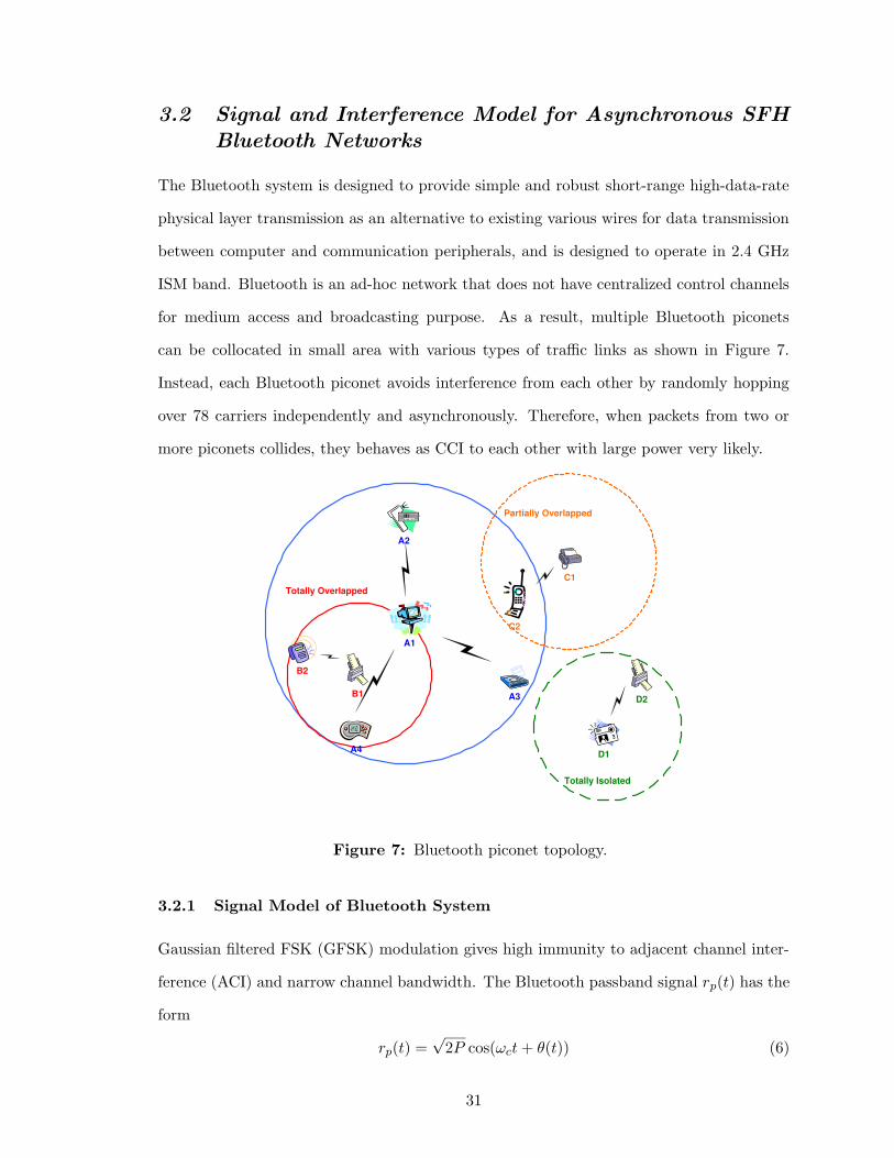
3.2 Signal and Interference Model for Asynchronous SFH

Bluetooth Networks

The Bluetooth system is designed to provide simple and robust short-range high-data-rate

physical layer transmission as an alternative to existing various wires for data transmission

between computer and communication peripherals, and is designed to operate in 2.4 GHz

ISM band. Bluetooth is an ad-hoc network that does not have centralized control channels

for medium access and broadcasting purpose. As a result, multiple Bluetooth piconets

can be collocated in small area with various types of traffic links as shown in Figure 7.

Instead, each Bluetooth piconet avoids interference from each other by randomly hopping

over 78 carriers independently and asynchronously. Therefore, when packets from two or

more piconets collides, they behaves as CCI to each other with large power very likely.

Totally Overlapped

Partially Overlapped

Totally Isolated

B1

C2

C1

A2

D1 A4

A3

B2

A1

D2

Figure 7: Bluetooth piconet topology.

3.2.1 Signal Model of Bluetooth System

Gaussian filtered FSK (GFSK) modulation gives high immunity to adjacent channel inter-

ference (ACI) and narrow channel bandwidth. The Bluetooth passband signal rp(t) has the

form

rp(t) =√

2P cos(ωct + θ(t)) (6)

31

where P is the signal power, ωc = 2πfc is the angular frequency, and

θ(t) = 2πh

∫ t

−∞

∞∑

i=−∞

sig(τ − iT )dτ (7)

where the si ∈ {±1} are binary data symbols, h is the modulation index, T is the symbol

duration, and g(t) is the response of a Gaussian low-pass filter to a rectangular pulse of

duration T . The Gaussian shaping pulse is

g(t) =1

2T

[

Q

(

2πBgT−t

T√

ln 2

)

−Q

(

2πBgT(−t + T )

T√

ln 2

)]

(8)

where Q(·) is the normalized cumulative normal distribution, and BgT is the normalized 3

dB bandwidth of the Gaussian low-pass filter. In Bluetooth, a small modulation index of

0.28 < h < 0.35 and a normalized bandwidth of BgT = 0.5 are used. Since the Gaussian

shaping pulse is longer than the baud duration, intersymbol interference (ISI) is introduced,

but the GFSK pulse also gives the advantage of lower side lobes in the frequency domain

than other modulation schemes.

Bluetooth receivers usually employ a low-cost noncoherent frequency discriminator re-

ceiver. The frequency discriminator consists of a differentiator followed by an envelope

detector, and its output is proportional to baseband signal r(t) [128]. The received complex

baseband equivalent signal at the output of the frequency discriminator is

r(t) =∞∑

i=−∞

sig(t− iT )h(t− iT − τ) + n(t)

=

∞∑

i=−∞

a(t)sig(t− iT − τ) + n(t). (9)

where h(t) = a(t)δ(t) is the channel impulse response with the assumption of flat fading over

each subbands. Under the condition of high carrier-to-noise ratio, the additive narrow-band

noise, n(t), can be written as

n(t) =1

2πAc

dnQ(t)

dt(10)

where Ac is the carrier amplitude and nQ(t) is the quadrature component of complex Gaus-

sian noise having zero mean and power spectral density N0. The corresponding power

32

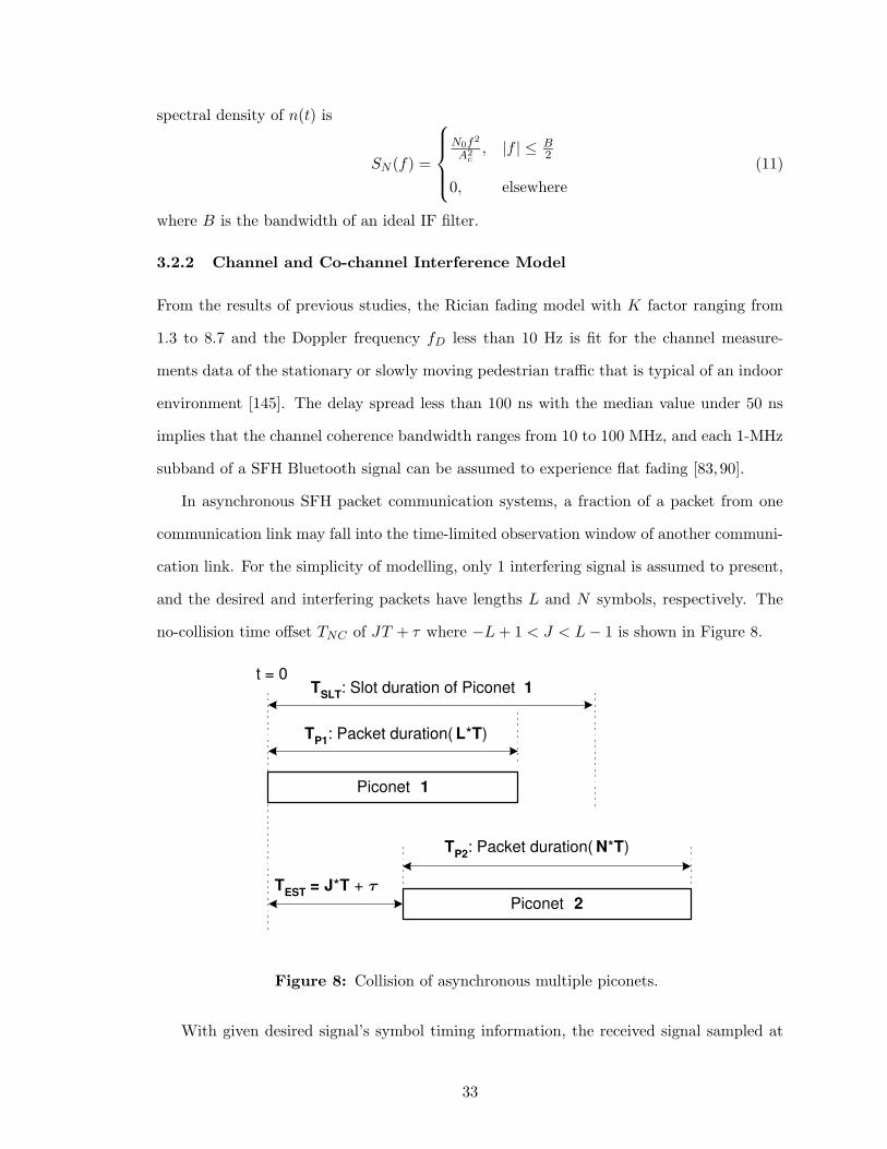
spectral density of n(t) is

SN (f) =

N0f2

A2c

, |f | ≤ B2

0, elsewhere

(11)

where B is the bandwidth of an ideal IF filter.

3.2.2 Channel and Co-channel Interference Model

From the results of previous studies, the Rician fading model with K factor ranging from

1.3 to 8.7 and the Doppler frequency fD less than 10 Hz is fit for the channel measure-

ments data of the stationary or slowly moving pedestrian traffic that is typical of an indoor

environment [145]. The delay spread less than 100 ns with the median value under 50 ns

implies that the channel coherence bandwidth ranges from 10 to 100 MHz, and each 1-MHz

subband of a SFH Bluetooth signal can be assumed to experience flat fading [83,90].

In asynchronous SFH packet communication systems, a fraction of a packet from one

communication link may fall into the time-limited observation window of another communi-

cation link. For the simplicity of modelling, only 1 interfering signal is assumed to present,

and the desired and interfering packets have lengths L and N symbols, respectively. The

no-collision time offset TNC of JT + τ where −L + 1 < J < L− 1 is shown in Figure 8.

T SLT : Slot duration of Piconet 1

T P1 : Packet duration( L * T )

Piconet 2

Piconet 1

T EST = J * T +

T P2 : Packet duration( N * T )

t = 0

PSfrag replacementsτ

Figure 8: Collision of asynchronous multiple piconets.

With given desired signal’s symbol timing information, the received signal sampled at

33

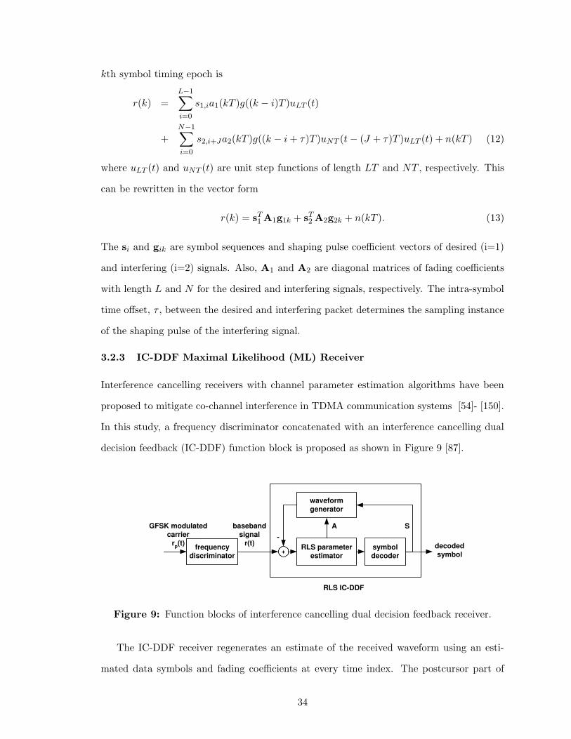
kth symbol timing epoch is

r(k) =L−1∑

i=0

s1,ia1(kT )g((k − i)T )uLT (t)

+N−1∑

i=0

s2,i+Ja2(kT )g((k − i + τ)T )uNT (t− (J + τ)T )uLT (t) + n(kT ) (12)

where uLT (t) and uNT (t) are unit step functions of length LT and NT , respectively. This

can be rewritten in the vector form

r(k) = sT1 A1g1k + sT

2 A2g2k + n(kT ). (13)

The si and gik are symbol sequences and shaping pulse coefficient vectors of desired (i=1)

and interfering (i=2) signals. Also, A1 and A2 are diagonal matrices of fading coefficients

with length L and N for the desired and interfering signals, respectively. The intra-symbol

time offset, τ , between the desired and interfering packet determines the sampling instance

of the shaping pulse of the interfering signal.

3.2.3 IC-DDF Maximal Likelihood (ML) Receiver

Interference cancelling receivers with channel parameter estimation algorithms have been

proposed to mitigate co-channel interference in TDMA communication systems [54]- [150].

In this study, a frequency discriminator concatenated with an interference cancelling dual

decision feedback (IC-DDF) function block is proposed as shown in Figure 9 [87].

GFSK modulated carrier

r p (t)

waveform generator

RLS parameter estimator

+ frequency

discriminator symbol decoder

decoded symbol

RLS IC-DDF

baseband signal

r (t) -

A S

Figure 9: Function blocks of interference cancelling dual decision feedback receiver.

The IC-DDF receiver regenerates an estimate of the received waveform using an esti-

mated data symbols and fading coefficients at every time index. The postcursor part of

34

estimated signal is subtracted from the received signal to reduce the estimation error in

the truncated decision metric for the maximum likelihood receiver. The symbol vector

s(i) = [s1,i, s2,i]T is estimated at every symbol interval in a ML manner and the diagonal

matrix of fading coefficients A(k) is updated at every symbol interval by using a recursive

approach. Assuming that an interfering packet has collided with the desired packet be-

fore the kth symbol, the conditional PDF of the received signal rIC(k) at the input to the

IC-DDF ML receiver with pth estimated symbol pair, for p ∈ {1, 2, 3, 4}, is [150]

p(rIC(k)|sp(k),Ap(k)) =1

πNo(1 + Ep(k))exp

{

− 1

No(1 + Ep(k))|ep(k)|2

}

(14)

where

rIC(k) = r(k)−k−1∑

i=0

s1,ia1(kT )g((k − i)T )−k−1∑

i=0

s2,i+Ja2(kT )g((k − i + τ)T ) (15)

ep(k) = rIC(k)− rp(k) (16)

rp(k) = sTp (k)Ap(k)g0 (17)

Ep(k) = sTp (k)Pp(k|k − 1)sp(k). (18)

The variables in (14) to (18) are listed in Table 3. The normalized covariance matrix of

ap(k), Pp(k|k − 1), is

Pp(k|k − 1) = (Ap(k)− 〈A(k|k − 1)〉) · (Ap(k)− 〈A(k|k − 1)〉)T /No (19)

where 〈A(k|k − 1)〉 is an a priori average of the fading coefficients from the 0 to the

(k− 1)th symbols given s(k− 1) and rIC(k− 1). With the modified received signal rIC(k),

the estimation error ep(k) is free from the energy of the previous k − 1 symbols if the

estimation of previous symbols and fading coefficients are correct. The equivalent log-

likelihood decision metric for IC-DDF ML estimator is

µ(sp(k)) = − |ep(k)|2 . (20)

35

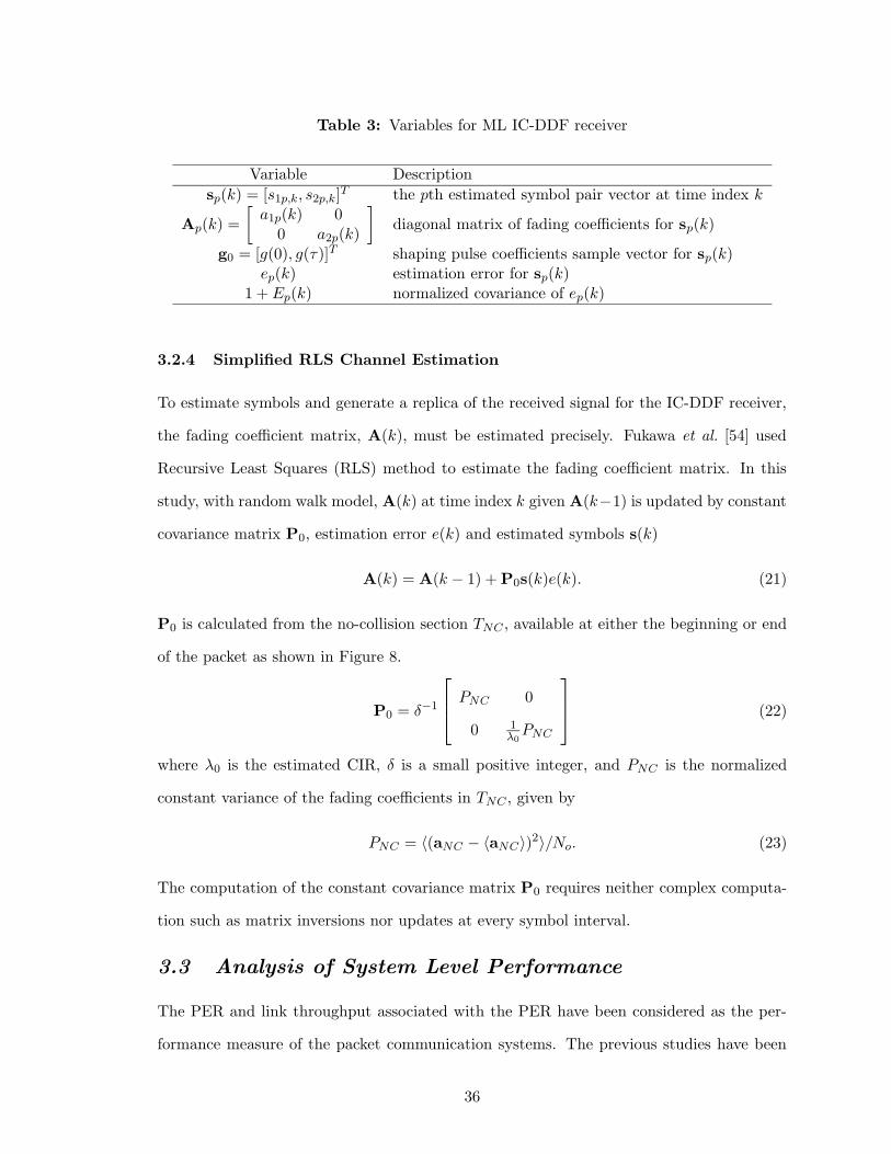
Table 3: Variables for ML IC-DDF receiver

Variable Description

sp(k) = [s1p,k, s2p,k]T the pth estimated symbol pair vector at time index k

Ap(k) =

[

a1p(k) 00 a2p(k)

]

diagonal matrix of fading coefficients for sp(k)

g0 = [g(0), g(τ)]T shaping pulse coefficients sample vector for sp(k)ep(k) estimation error for sp(k)

1 + Ep(k) normalized covariance of ep(k)

3.2.4 Simplified RLS Channel Estimation

To estimate symbols and generate a replica of the received signal for the IC-DDF receiver,

the fading coefficient matrix, A(k), must be estimated precisely. Fukawa et al. [54] used

Recursive Least Squares (RLS) method to estimate the fading coefficient matrix. In this

study, with random walk model, A(k) at time index k given A(k−1) is updated by constant

covariance matrix P0, estimation error e(k) and estimated symbols s(k)

A(k) = A(k − 1) + P0s(k)e(k). (21)

P0 is calculated from the no-collision section TNC , available at either the beginning or end

of the packet as shown in Figure 8.

P0 = δ−1

PNC 0

0 1λ0

PNC

(22)

where λ0 is the estimated CIR, δ is a small positive integer, and PNC is the normalized

constant variance of the fading coefficients in TNC , given by

PNC = 〈(aNC − 〈aNC〉)2〉/No. (23)

The computation of the constant covariance matrix P0 requires neither complex computa-

tion such as matrix inversions nor updates at every symbol interval.

3.3 Analysis of System Level Performance

The PER and link throughput associated with the PER have been considered as the per-

formance measure of the packet communication systems. The previous studies have been

36

focused on systematic approach to measure PER under different channel impairments of

multipath fading and co-channel interference [67,92,149,154].

However, all those analysis based on the BER data derived from conventional receiver

which has no co-channel interference cancellation capability. In this study, PER is derived

by integrating BER of interference cancelling receiver with statistics of CIR as well as

considering the capture effect in calculation of packet collision probability.

3.3.1 Packet Error Probability

When the multiple packets are transmitted through shared medium, the probability of

packet error is defined as follows.

Pr(e) = Pr(e|c)Pr(c) + Pr(e|nc)Pr(nc) (24)

where Pr(e|c) is the conditional probability of packet error given collision of probability

Pr(c), and Pr(e|nc) the conditional probability of packet error given no packet collision.

Because the Pr(e|nc) is very smaller than Pr(e|c) in high signal-to-noise ratio condition

which is very likely on short distance communication link, Pr(e|nc) is assumed zero.

With given CIR and the BER of interference cancelling receiver associated with it, the

PER depends on the length of the collision section in a packet, l and forward error correction

(FEC) function of the packet. Thus, the probability of packet error in (24) can be derived

from double integration of conditional probability of packet error (CPPE) with l = m and

Λ = λ

E[Pr(e)] = Pr(c)

∫

Rl

∫

RΛ

Pr(e|λ, m)fl(m|c)fΛ(λ)dλdm (25)

where fΛ(λ) and fl(m|c) are the PDF of the average received CIR and the conditional

PDF of collision length given collision, respectively. Since the time offset TNC is uniformly

distributed over TSLTS , fl(m|c) is

fl(m|c) =1

TSLTSfor m ∈ [0, TSLTS ]. (26)

The PDF of CIR, fΛ(λ) is derived from geometric arguments. Since the CIR is a function of

the path loss statistics and the relative distances from the intended receiver to the desired

37

and interfering transmitters, fΛ(λ) can be written as

fΛ(λ) =

∫

Rrd

fΛ(λ|σ)frd(σ)dσ (27)

where frd(σ) is the PDF of the distance from the desired transmitter to the receiver,rd, and

fΛ(λ|σ) is the conditional PDF of CIR given rd. Assuming that the intended receiver is

located at the center of the cell and the desired and interfering transmitters are uniformly

distributed over the piconet, frd(σ) is derived by following method. The probability that

desired transmitter is located in the annular ring defined by ri < σ < ro is

Pr(ri < σ < ro) ,area of ri < σ < ro

total cell area=

r2o − r2

i

R2(28)

where R is the radius of a piconet cell. The path-loss equation from a previous study used

in derivation of fΛ(λ|σ) [83]. The received power at distance d is

PRX(d) = P0 + 10a log10(d). (29)

where d is in meter, P0 is the path loss at 1 m distance, and a is the path loss exponent.

The measured value of P0 is 43.1 dB at 2.4 GHz, and the measured values of a are 1.86 and

3.33 for LOS (line-of-sight) and OBS (obstructed) channels, respectively. Figure 10 shows

the cumulative distribution functions (CDF) of CIR computed from (27)-(29) with different

visibility indices between transmitters and receivers.

An example of distribution of CIR of a typical frequency reuse cellular system is given

for comparison. Unlike the Bluetooth piconets, the frequency reuse scheme of conventional

cellular systems shifts the distribution to the right. As a result, the average received CIR

is located between 10 to 20 dB range. The CPPE given Λ = λ and l = m is

Pr(e|λ, m) = 1−[

Ne∑

i=0

(

NB

i

)

(ρb(λ))i(1− ρb(λ))NB−i

]Nm

(1− ρb(λ))NR (30)

where ρb(λ) is the BER at Λ = λ, and Ne is the maximum number of bit errors allowed in

one FEC block of length NB. The length of collision section m and NB decide the number

of FEC blocks, Nm, and residual bits, NR, in the collision section of a packet

Nm =

⌊

m

NB

⌋

(31)

NR = m−NBNm. (32)

38

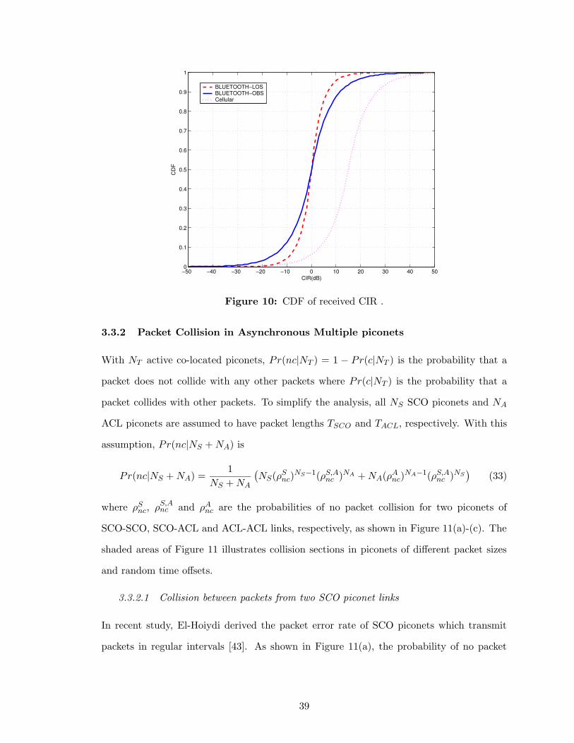
−50 −40 −30 −20 −10 0 10 20 30 40 500

0.1

0.2

0.3

0.4

0.5

0.6

0.7

0.8

0.9

1

CIR(dB)

CD

F

BLUETOOTH−LOSBLUETOOTH−OBSCellular

Figure 10: CDF of received CIR .

3.3.2 Packet Collision in Asynchronous Multiple piconets

With NT active co-located piconets, Pr(nc|NT ) = 1 − Pr(c|NT ) is the probability that a

packet does not collide with any other packets where Pr(c|NT ) is the probability that a

packet collides with other packets. To simplify the analysis, all NS SCO piconets and NA

ACL piconets are assumed to have packet lengths TSCO and TACL, respectively. With this

assumption, Pr(nc|NS + NA) is

Pr(nc|NS + NA) =1

NS + NA

(

NS(ρSnc)

NS−1(ρS,Anc )NA + NA(ρA

nc)NA−1(ρS,A

nc )NS)

(33)

where ρSnc, ρS,A

nc and ρAnc are the probabilities of no packet collision for two piconets of

SCO-SCO, SCO-ACL and ACL-ACL links, respectively, as shown in Figure 11(a)-(c). The

shaded areas of Figure 11 illustrates collision sections in piconets of different packet sizes

and random time offsets.

3.3.2.1 Collision between packets from two SCO piconet links

In recent study, El-Hoiydi derived the packet error rate of SCO piconets which transmit

packets in regular intervals [43]. As shown in Figure 11(a), the probability of no packet

39

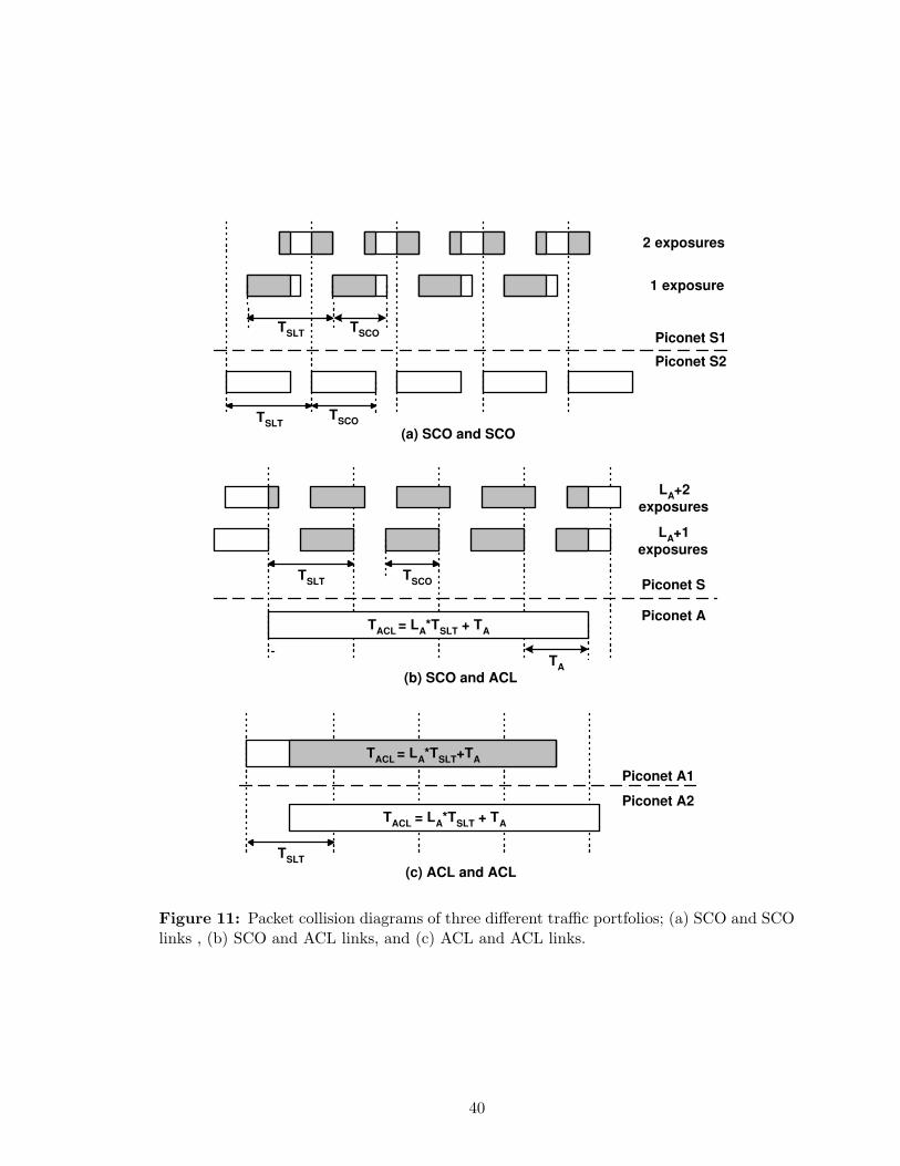
2 exposures

1 exposure

T SLT

Piconet S1

Piconet S2

T SCO

T SLT T SCO

(a) SCO and SCO

Piconet S

Piconet A

L A +1 exposures

L A +2 exposures

T A

T SCO T SLT

T ACL = L A *T SLT + T A

(b) SCO and ACL

Piconet A1

Piconet A2 T ACL = L A *T SLT + T A

T SLT (c) ACL and ACL

T ACL = L A *T SLT +T A

Figure 11: Packet collision diagrams of three different traffic portfolios; (a) SCO and SCOlinks , (b) SCO and ACL links, and (c) ACL and ACL links.

40

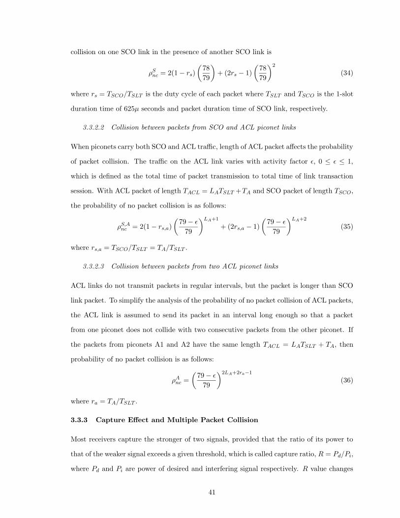
collision on one SCO link in the presence of another SCO link is

ρSnc = 2(1− rs)

(

78

79

)

+ (2rs − 1)

(

78

79

)2

(34)

where rs = TSCO/TSLT is the duty cycle of each packet where TSLT and TSCO is the 1-slot

duration time of 625µ seconds and packet duration time of SCO link, respectively.

3.3.2.2 Collision between packets from SCO and ACL piconet links

When piconets carry both SCO and ACL traffic, length of ACL packet affects the probability

of packet collision. The traffic on the ACL link varies with activity factor ε, 0 ≤ ε ≤ 1,

which is defined as the total time of packet transmission to total time of link transaction

session. With ACL packet of length TACL = LATSLT +TA and SCO packet of length TSCO,

the probability of no packet collision is as follows:

ρS,Anc = 2(1− rs,a)

(

79− ε

79

)LA+1

+ (2rs,a − 1)

(

79− ε

79

)LA+2

(35)

where rs,a = TSCO/TSLT = TA/TSLT .

3.3.2.3 Collision between packets from two ACL piconet links

ACL links do not transmit packets in regular intervals, but the packet is longer than SCO

link packet. To simplify the analysis of the probability of no packet collision of ACL packets,

the ACL link is assumed to send its packet in an interval long enough so that a packet

from one piconet does not collide with two consecutive packets from the other piconet. If

the packets from piconets A1 and A2 have the same length TACL = LATSLT + TA, then

probability of no packet collision is as follows:

ρAnc =

(

79− ε

79

)2LA+2ra−1

(36)

where ra = TA/TSLT .

3.3.3 Capture Effect and Multiple Packet Collision

Most receivers capture the stronger of two signals, provided that the ratio of its power to

that of the weaker signal exceeds a given threshold, which is called capture ratio, R = Pd/Pi,

where Pd and Pi are power of desired and interfering signal respectively. R value changes

41

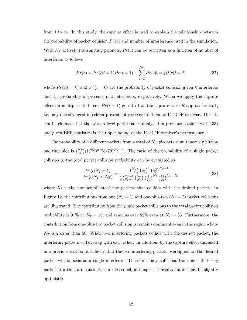
from 1 to ∞. In this study, the capture effect is used to explain the relationship between

the probability of packet collision Pr(c) and number of interference used in the simulation.

With NT actively transmitting piconets, Pr(c) can be rewritten as a function of number of

interferers as follows

Pr(c) = Pr(c|i = 1)Pr(i = 1) +

NT∑

j=2

Pr(c|i = j)Pr(i = j) (37)

where Pr(c|i = k) and Pr(i = k) are the probability of packet collision given k interferers

and the probability of presence of k interferers, respectively. When we apply the capture

effect on multiple interferers, Pr(i = 1) goes to 1 as the capture ratio R approaches to 1,

i.e, only one strongest interferer presents at receiver front end of IC-DDF receiver. Thus, it

can be claimed that the system level performance analyzed in previous sessions with (33)

and given BER statistics is the upper bound of the IC-DDF receiver’s performance.

The probability of n different packets from a total of NT piconets simultaneously hitting

one time slot is(

NT

n

)

(1/79)n(78/79)NT−n. The ratio of the probability of a single packet

collision to the total packet collision probability can be evaluated as

Pr(c|NI = 1)

Pr(c|NI < NT )=

(

NT

1

) (

179

)1 (7879

)NT−1

∑NT−1NI=1

(

NT

NI

) (

179

)NI(

7879

)NT−NI(38)

where NI is the number of interfering packets that collides with the desired packet. In

Figure 12, the contributions from one (NI = 1) and one-plus-two (NI = 2) packet collisions

are illustrated. The contribution from the single packet collisions to the total packet collision

probability is 91% at NT = 15, and remains over 82% even at NT = 35. Furthermore, the

contribution from one-plus-two packet collision is remains dominant even in the region where

NT is greater than 50. When two interfering packets collide with the desired packet, the

interfering packets will overlap with each other. In addition, by the capture effect discussed

in a previous section, it is likely that the two interfering packets overlapped on the desired

packet will be seen as a single interferer. Therefore, only collisions from one interfering

packet at a time are considered in the sequel, although the results obtain may be slightly

optimistic.

42

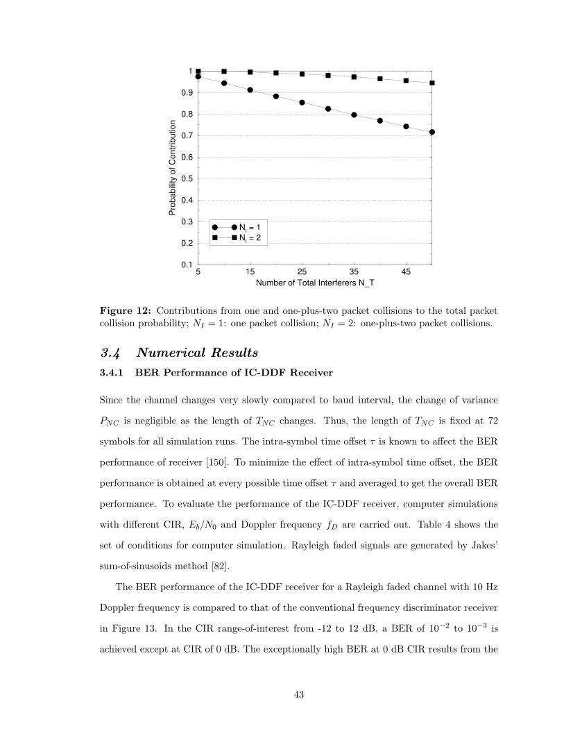
5 15 25 35 45Number of Total Interferers N_T

0.1

0.2

0.3

0.4

0.5

0.6

0.7

0.8

0.9

1

Pro

babi

lity

of C

ontri

butio

n

NI = 1NI = 2

Figure 12: Contributions from one and one-plus-two packet collisions to the total packetcollision probability; NI = 1: one packet collision; NI = 2: one-plus-two packet collisions.

3.4 Numerical Results

3.4.1 BER Performance of IC-DDF Receiver

Since the channel changes very slowly compared to baud interval, the change of variance

PNC is negligible as the length of TNC changes. Thus, the length of TNC is fixed at 72

symbols for all simulation runs. The intra-symbol time offset τ is known to affect the BER

performance of receiver [150]. To minimize the effect of intra-symbol time offset, the BER

performance is obtained at every possible time offset τ and averaged to get the overall BER

performance. To evaluate the performance of the IC-DDF receiver, computer simulations

with different CIR, Eb/N0 and Doppler frequency fD are carried out. Table 4 shows the

set of conditions for computer simulation. Rayleigh faded signals are generated by Jakes’

sum-of-sinusoids method [82].

The BER performance of the IC-DDF receiver for a Rayleigh faded channel with 10 Hz

Doppler frequency is compared to that of the conventional frequency discriminator receiver

in Figure 13. In the CIR range-of-interest from -12 to 12 dB, a BER of 10−2 to 10−3 is

achieved except at CIR of 0 dB. The exceptionally high BER at 0 dB CIR results from the

43

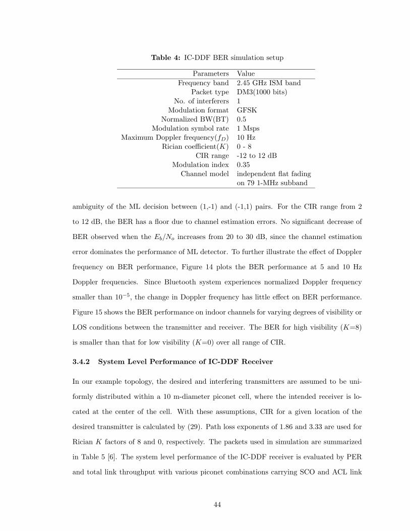
Table 4: IC-DDF BER simulation setup

Parameters Value

Frequency band 2.45 GHz ISM bandPacket type DM3(1000 bits)

No. of interferers 1Modulation format GFSK

Normalized BW(BT) 0.5Modulation symbol rate 1 Msps

Maximum Doppler frequency(fD) 10 HzRician coefficient(K) 0 - 8

CIR range -12 to 12 dBModulation index 0.35

Channel model independent flat fadingon 79 1-MHz subband

ambiguity of the ML decision between (1,-1) and (-1,1) pairs. For the CIR range from 2

to 12 dB, the BER has a floor due to channel estimation errors. No significant decrease of

BER observed when the Eb/No increases from 20 to 30 dB, since the channel estimation

error dominates the performance of ML detector. To further illustrate the effect of Doppler

frequency on BER performance, Figure 14 plots the BER performance at 5 and 10 Hz

Doppler frequencies. Since Bluetooth system experiences normalized Doppler frequency

smaller than 10−5, the change in Doppler frequency has little effect on BER performance.

Figure 15 shows the BER performance on indoor channels for varying degrees of visibility or

LOS conditions between the transmitter and receiver. The BER for high visibility (K=8)

is smaller than that for low visibility (K=0) over all range of CIR.

3.4.2 System Level Performance of IC-DDF Receiver

In our example topology, the desired and interfering transmitters are assumed to be uni-

formly distributed within a 10 m-diameter piconet cell, where the intended receiver is lo-

cated at the center of the cell. With these assumptions, CIR for a given location of the

desired transmitter is calculated by (29). Path loss exponents of 1.86 and 3.33 are used for

Rician K factors of 8 and 0, respectively. The packets used in simulation are summarized

in Table 5 [6]. The system level performance of the IC-DDF receiver is evaluated by PER

and total link throughput with various piconet combinations carrying SCO and ACL link

44

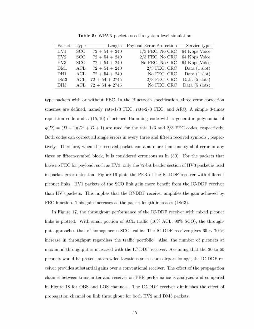
Table 5: WPAN packets used in system level simulation

Packet Type Length Payload Error Protection Service type

HV1 SCO 72 + 54 + 240 1/3 FEC, No CRC 64 Kbps VoiceHV2 SCO 72 + 54 + 240 2/3 FEC, No CRC 64 Kbps VoiceHV3 SCO 72 + 54 + 240 No FEC, No CRC 64 Kbps VoiceDM1 ACL 72 + 54 + 240 2/3 FEC, CRC Data (1 slot)DH1 ACL 72 + 54 + 240 No FEC, CRC Data (1 slot)DM3 ACL 72 + 54 + 2745 2/3 FEC, CRC Data (5 slots)DH3 ACL 72 + 54 + 2745 No FEC, CRC Data (5 slots)

type packets with or without FEC. In the Bluetooth specification, three error correction

schemes are defined, namely rate-1/3 FEC, rate-2/3 FEC, and ARQ. A simple 3-times

repetition code and a (15, 10) shortened Hamming code with a generator polynomial of

g(D) = (D + 1)(D4 + D + 1) are used for the rate 1/3 and 2/3 FEC codes, respectively.

Both codes can correct all single errors in every three and fifteen received symbols , respec-

tively. Therefore, when the received packet contains more than one symbol error in any

three or fifteen-symbol block, it is considered erroneous as in (30). For the packets that

have no FEC for payload, such as HV3, only the 72-bit header section of HV3 packet is used

in packet error detection. Figure 16 plots the PER of the IC-DDF receiver with different

piconet links. HV1 packets of the SCO link gain more benefit from the IC-DDF receiver

than HV3 packets. This implies that the IC-DDF receiver amplifies the gain achieved by

FEC function. This gain increases as the packet length increases (DM3).

In Figure 17, the throughput performance of the IC-DDF receiver with mixed piconet

links is plotted. With small portion of ACL traffic (10% ACL, 90% SCO), the through-

put approaches that of homogeneous SCO traffic. The IC-DDF receiver gives 60 ∼ 70 %

increase in throughput regardless the traffic portfolio. Also, the number of piconets at

maximum throughput is increased with the IC-DDF receiver. Assuming that the 30 to 60

piconets would be present at crowded locations such as an airport lounge, the IC-DDF re-

ceiver provides substantial gains over a conventional receiver. The effect of the propagation

channel between transmitter and receiver on PER performance is analyzed and compared

in Figure 18 for OBS and LOS channels. The IC-DDF receiver diminishes the effect of

propagation channel on link throughput for both HV2 and DM3 packets.

45

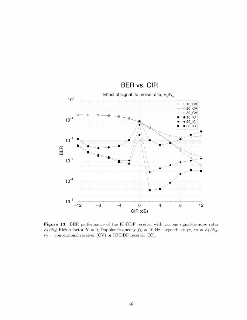
−12 −8 −4 0 4 8 12CIR (dB)

10−5

10−4

10−3

10−2

10−1

100

BE

R

BER vs. CIREffect of signal−to−noise ratio, Eb/No

10_CV20_CV30_CV10_IC20_IC30_IC

Figure 13: BER performance of the IC-DDF receiver with various signal-to-noise ratioEb/No; Rician factor K = 0, Doppler frequency fD = 10 Hz. Legend: xx yy, xx = Eb/No,yy = conventional receiver (CV) or IC-DDF receiver (IC).

46

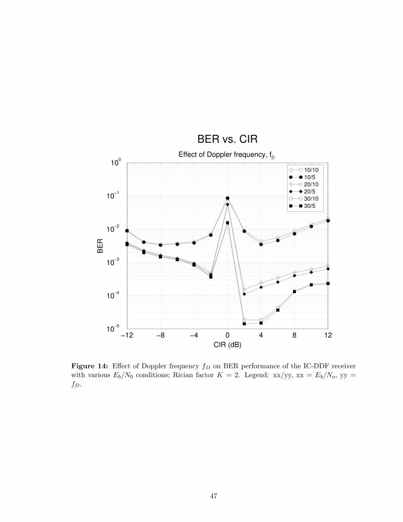
−12 −8 −4 0 4 8 12CIR (dB)

10−5

10−4

10−3

10−2

10−1

100

BE

R

BER vs. CIREffect of Doppler frequency, fD

10/1010/520/1020/530/1030/5

Figure 14: Effect of Doppler frequency fD on BER performance of the IC-DDF receiverwith various Eb/N0 conditions; Rician factor K = 2. Legend: xx/yy, xx = Eb/No, yy =fD.

47

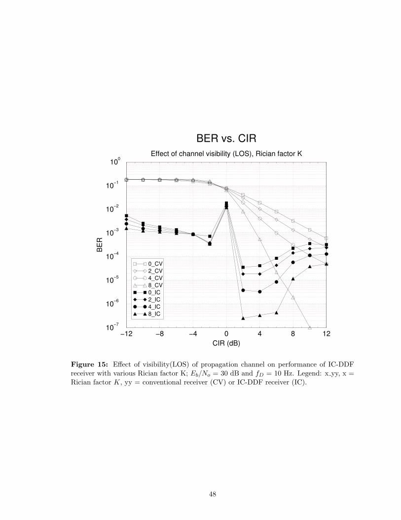
−12 −8 −4 0 4 8 12CIR (dB)

10−7

10−6

10−5

10−4

10−3

10−2

10−1

100

BE

R

BER vs. CIREffect of channel visibility (LOS), Rician factor K

0_CV2_CV4_CV8_CV0_IC2_IC4_IC8_IC

Figure 15: Effect of visibility(LOS) of propagation channel on performance of IC-DDFreceiver with various Rician factor K; Eb/No = 30 dB and fD = 10 Hz. Legend: x yy, x =Rician factor K, yy = conventional receiver (CV) or IC-DDF receiver (IC).

48

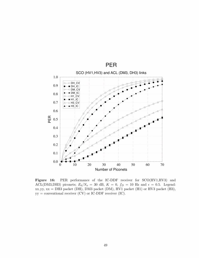
0 10 20 30 40 50 60 70Number of Piconets

0.0

0.1

0.2

0.3

0.4

0.5

0.6

0.7

0.8

0.9

1.0

PE

R

PERSCO (HV1,HV3) and ACL (DM3, DH3) links

DH_CVDH_ICDM_CVDM_ICH1_CVH1_ICH3_CVH3_IC

Figure 16: PER performance of the IC-DDF receiver for SCO(HV1,HV3) andACL(DM3,DH3) piconets; Eb/No = 30 dB, K = 0, fD = 10 Hz and ε = 0.5. Legend:xx yy, xx = DH3 packet (DH), DM3 packet (DM), HV1 packet (H1) or HV3 packet (H3),yy = conventional receiver (CV) or IC-DDF receiver (IC).

49

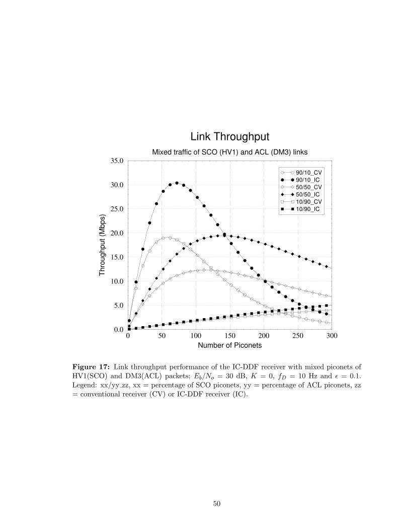
0 50 100 150 200 250 300Number of Piconets

0.0

5.0

10.0

15.0

20.0

25.0

30.0

35.0

Thro

ughp

ut (M

bps)

Link ThroughputMixed traffic of SCO (HV1) and ACL (DM3) links

90/10_CV90/10_IC50/50_CV50/50_IC10/90_CV10/90_IC

Figure 17: Link throughput performance of the IC-DDF receiver with mixed piconets ofHV1(SCO) and DM3(ACL) packets; Eb/No = 30 dB, K = 0, fD = 10 Hz and ε = 0.1.Legend: xx/yy zz, xx = percentage of SCO piconets, yy = percentage of ACL piconets, zz= conventional receiver (CV) or IC-DDF receiver (IC).

50

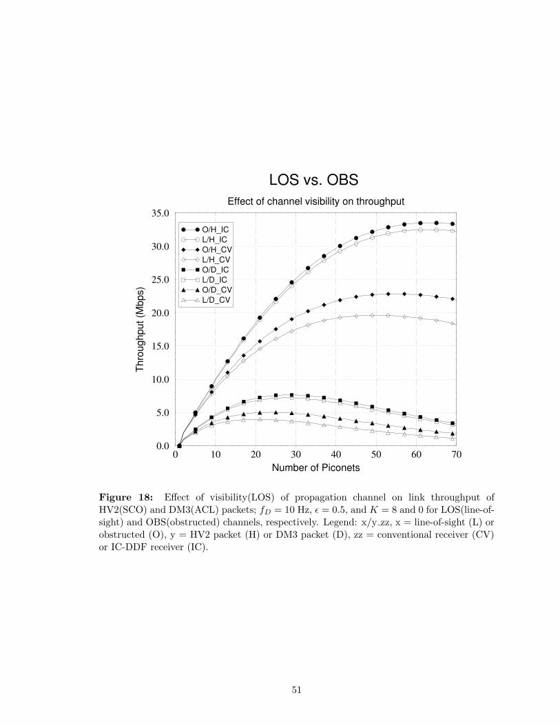
0 10 20 30 40 50 60 70Number of Piconets

0.0

5.0

10.0

15.0

20.0

25.0

30.0

35.0

Thro

ughp

ut (M

bps)

LOS vs. OBS Effect of channel visibility on throughput

O/H_ICL/H_ICO/H_CVL/H_CVO/D_ICL/D_ICO/D_CVL/D_CV

Figure 18: Effect of visibility(LOS) of propagation channel on link throughput ofHV2(SCO) and DM3(ACL) packets; fD = 10 Hz, ε = 0.5, and K = 8 and 0 for LOS(line-of-sight) and OBS(obstructed) channels, respectively. Legend: x/y zz, x = line-of-sight (L) orobstructed (O), y = HV2 packet (H) or DM3 packet (D), zz = conventional receiver (CV)or IC-DDF receiver (IC).

51

CHAPTER IV

JOINT DETECTION INTERFERENCE REJECTION

COMBINING GSM/EDGE RECEIVER

4.1 Introduction

Co-channel interference (CCI) is the primary impediment in cellular frequency reuse sys-

tems. Single antenna interference mitigating receivers that use serial/parallel interference

cancellation (SIC/PIC), joint detection (JD), and other multiuser detection (MUD) algo-

rithms have been proposed [93]. Multiple antenna receivers have also been proposed to

suppress CCI by using optimal combining [146]. A receiver that combines interference re-

jection combining (IRC) with maximum likelihood sequence estimation (MLSE) has been

proposed for channels exhibiting both CCI and intersymbol interference (ISI) [28]. For

channels with long delay spreads, the MLSE decoding is impractical because of increasing

complexity, especially for the systems with large signal constellation sets. The delayed deci-

sion feedback sequence estimation (DDFSE) scheme is proposed as an alternative solution

with reduced complexity at the expense of minute gains [18,41,84].

In frequency reuse cellular systems, the received carrier-to-interference ratio is expected

to be greater than 0 dB by its network topology, and most interference cancelling receivers

are designed to mitigate the CCI weaker than the desired signal. However, when a receiver

tries to reach remote BSs for applications such as intelligence or emergency operations,

the receiver should be operable in CIR far below the range that conventional receivers are

not usually designed to operate in, CIR < 0 dB. Furthermore, multipath fading, non-ideal

terrain structures makes decoding of the desired signal more challenging.

This study proposes a soft output fractionally spaced joint detection IRC-DDFSE (JD

IRC-DDFSE) receiver. The trellis search technique used in the IRC-DDFSE receiver in

[84] is extended to perform joint detection of two co-channel signals, while IRC is used

52

to reject the remaining co-channel interference. Moreover, the JD IRC-DDFSE receiver

generates soft-outputs that are used as inputs to a soft decision channel decoder by using

Log-MAP algorithm. This modification permits the receiver to recover signals in very

strong CCI, where the received CIR may even be less than 0 dB. The precision of soft-

outputs generated by the Log-MAP algorithm in DDFSE function is improved by using

the surviving sequence and the covariance matrix estimated from concatenated Viterbi

algorithm. Also, the contribution of this study includes a joint least squares (LS) channel

estimation which enables the receiver estimate the channel information of the desired signal

in low-CIR conditions. Joint channel estimation also reduces the side effect of the timing

offset between the co-channel signals.

A narrow beam adaptive antenna (NBAA) array can be used to reduce the number of

co-channel signals [15, 81]. In a cellular topology, for example, an NBAA aligned to the

line-of-sight (LOS) path from the receiver to the target BS as shown in Figure 19, admits

one dominant co-channel signal from the closest tier, plus a few highly attenuated co-

channel signals from outer tiers. In contrast, a conventional 120◦ wide-beam sector antenna

receives two strong co-channel signals from the nearest tier. This study shows that the

combination of an NBAA with JD IRC-DDFSE is highly effective for mitigating co-channel

interference. In fact, this arrangement may provide sufficient interference rejection to allow

communication with a distant base station in the presence of a near-by co-channel base

station. Such capabilities may be useful for intelligence or emergency operations in cellular

networks.

The remainder of this chapter is organized as follows. Section 4.2 introduces the system

model with an NBAA array. Section 4.3 details the soft-output fractionally-spaced JD

IRC-DDFSE receiver, and presents methods for joint channel estimation technique and

soft-output generation. In Section 4.4, the impact of imbalanced CIR observed in receive

branches is investigated. Section 4.5 discusses the receiver performance for binary and

non-binary 8-PSK modulated systems.

53

4.2 System Model for Range Extended Reception

4.2.1 Signal Model

The system under consideration can be modelled as a K-input, J-ouptut, channel, where

K is the number of co-channel signals and J the number of receiver antenna units. We

arbitrarily assign the first user (k = 1) as the desired signal while the other users k =

2, . . . , K are the interfering co-channel signals. The signal at the output of the jth receiver

antenna unit is

r(j)(t) =K∑

k=1

∞∑

`=−∞

x(k)` h(k,j)(t− `T − τk) + η(j)(t) , (39)

where η(j)(t) is zero-mean complex additive white Gaussian noise process with variance

σ2η = 1

2E[|η(j)(t)|2] = No watts/Hz, and x(k) = {x(k)` } is the sequence of complex symbols

transmitted by the kth co-channel user. The overall channel response h(k,j)(t) is the con-

volution of a complex channel impulse response c(k,j)(t) and the transmitting filter ha(t).

For the synchronous GSM network considered in this study, the delay offsets τk for all co-

channel signals will be at most two symbol intervals [20]. The influence of the delay offsets

of 0 to 2 symbol duration will be evaluated by computer simulation in Section IV. Joint

channel estimation is performed using the known training symbol sequences (TSS) followed

by joint detection.

4.2.2 NBAA Preprocessing

As shown in Figure 19, we consider a cellular topology where a range extended intercept

receiver (MS) located in one co-channel BS area (BS7) tries to communicate with a co-

channel BS in the outer tier (BS1). There are 3 predominate co-channel BSs, namely BS2,

BS3, and BS4, where the angle α between BS2 and BS4 as seen from the intercept receiver

is approximately 60◦. A practical NBAA array can reject all CCI signals, leaving only one

strong source of CCI (BS3) which is located on the LOS path from MS to BS1. In contrast,

a conventional 120◦ wide-beam sector antenna will see at least 2 strong sources of CCI from

BSs in the first tier. In addition, both the NBAA array and wide-beam sector antennas

will receive additional CCI from the third and higher tiers (for example from BS8 and BS9)

but with a very small power level due to path loss attenuation. Finally, for NBAA arrays

54

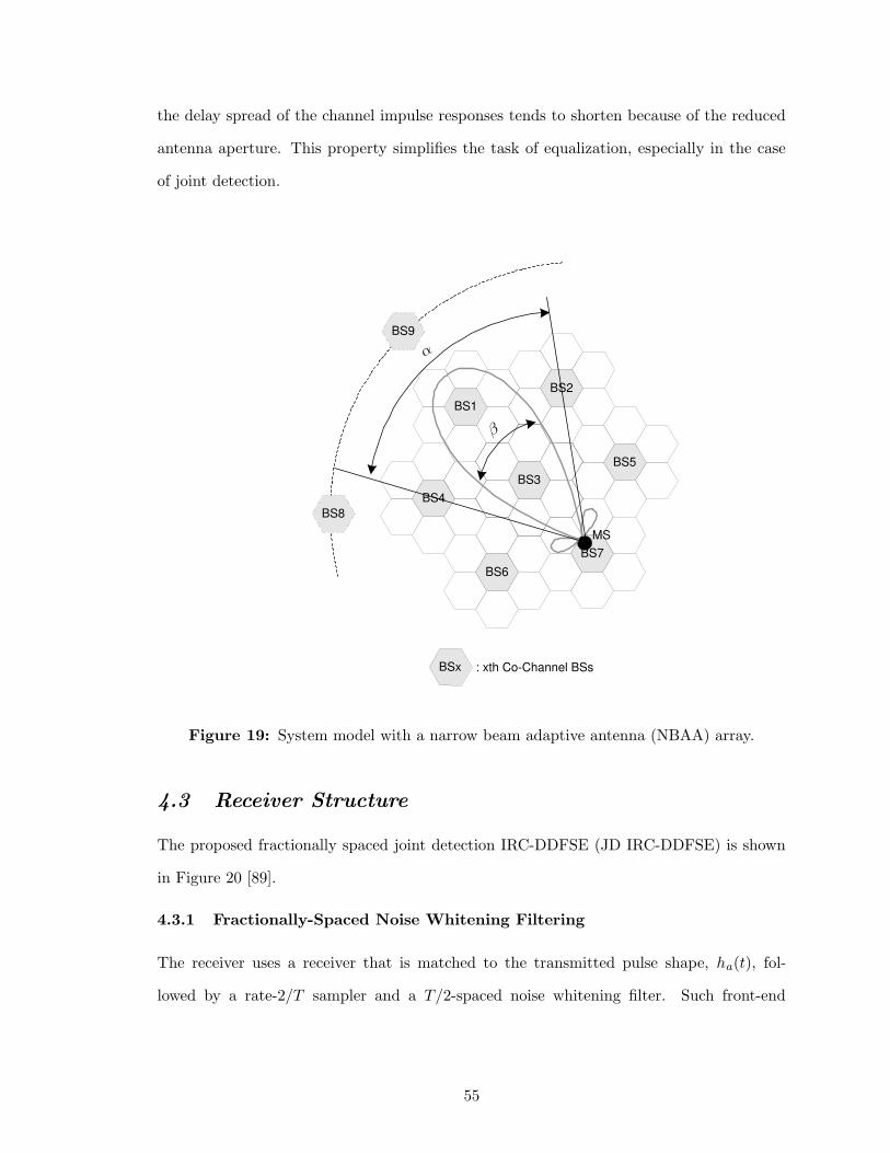
the delay spread of the channel impulse responses tends to shorten because of the reduced

antenna aperture. This property simplifies the task of equalization, especially in the case

of joint detection.

BS2

BS7 BS6

BS4

BS1

BS5 BS3

MS

BSx : xth Co-Channel BSs

BS8

BS9

PSfrag replacements

α

β

Figure 19: System model with a narrow beam adaptive antenna (NBAA) array.

4.3 Receiver Structure

The proposed fractionally spaced joint detection IRC-DDFSE (JD IRC-DDFSE) is shown

in Figure 20 [89].

4.3.1 Fractionally-Spaced Noise Whitening Filtering

The receiver uses a receiver that is matched to the transmitted pulse shape, ha(t), fol-

lowed by a rate-2/T sampler and a T/2-spaced noise whitening filter. Such front-end

55

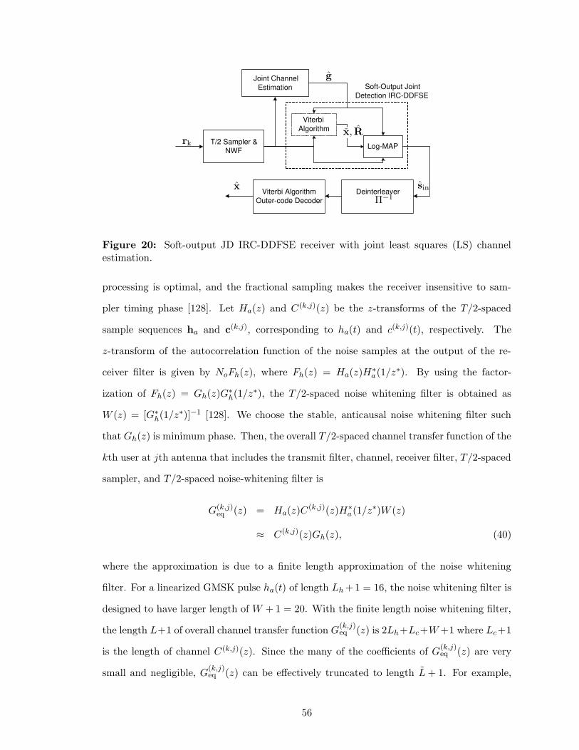
T/2 Sampler & NWF

Viterbi Algorithm Outer-code Decoder

Deinterleaver

Joint Channel Estimation Soft-Output Joint

Detection IRC-DDFSE

Viterbi Algorithm

Log-MAP

PSfrag replacements

g

sinx

rk

Π−1

x, R

Figure 20: Soft-output JD IRC-DDFSE receiver with joint least squares (LS) channelestimation.

processing is optimal, and the fractional sampling makes the receiver insensitive to sam-

pler timing phase [128]. Let Ha(z) and C(k,j)(z) be the z-transforms of the T/2-spaced

sample sequences ha and c(k,j), corresponding to ha(t) and c(k,j)(t), respectively. The

z-transform of the autocorrelation function of the noise samples at the output of the re-

ceiver filter is given by NoFh(z), where Fh(z) = Ha(z)H∗a(1/z∗). By using the factor-

ization of Fh(z) = Gh(z)G∗h(1/z∗), the T/2-spaced noise whitening filter is obtained as

W (z) = [G∗h(1/z∗)]−1 [128]. We choose the stable, anticausal noise whitening filter such

that Gh(z) is minimum phase. Then, the overall T/2-spaced channel transfer function of the

kth user at jth antenna that includes the transmit filter, channel, receiver filter, T/2-spaced

sampler, and T/2-spaced noise-whitening filter is

G(k,j)eq (z) = Ha(z)C(k,j)(z)H∗

a(1/z∗)W (z)

≈ C(k,j)(z)Gh(z), (40)

where the approximation is due to a finite length approximation of the noise whitening

filter. For a linearized GMSK pulse ha(t) of length Lh +1 = 16, the noise whitening filter is

designed to have larger length of W + 1 = 20. With the finite length noise whitening filter,

the length L+1 of overall channel transfer function G(k,j)eq (z) is 2Lh+Lc+W +1 where Lc+1

is the length of channel C(k,j)(z). Since the many of the coefficients of G(k,j)eq (z) are very

small and negligible, G(k,j)eq (z) can be effectively truncated to length L + 1. For example,

56

the effective length of the overall T/2-spaced channel can be set to 7 symbol durations, i.e.,

L + 1 = 14 for GSM/EDGE as in [59].

4.3.2 Joint Detection IRC-DDFSE

Let X(k)(z) and V (k,j)(z) be the z-transform of the input sequence and received signal from

the kth user at jth antenna unit, respectively, and V (k,j)(z) = G(k,j)eq (z)X(k)(z). Then, the

received signal samples at the output of the matched filter on the jth antenna unit are

r(j)2`+q =

K∑

k=1

v(k,j)2`+q + η

(j)2`+q

=K∑

k=1

(

µ∑

n=0

g(k,j)eq,2n+qx

(k)`−n + v

(k,j)+2`+q

)

+ η(j)2`+q, q = 0, 1 (41)

where v(k,j)+2`+q is the signal term from the channel impulse response longer than µ, and where

µ is the truncation length used in the DDFSE algorithm [41].

The proposed receiver jointly detects N co-channel signals, while the remaining K −N

co-channel signals plus additive white gaussian noise are treated as impairments. Equa-

tion (41) can be rewritten as

r(j)2`+q =

N∑

k=1

(

µ∑

n=0

g(k,j)eq,2n+qx

(k)`−n + v

(k,j)+2`+q

)

+ n(j)2`+q, q = 0, 1 (42)

where n(j)2`+q is the impairment

n(j)2`+q =

K∑

k=N+1

L/2∑

n=0

g(k,j)eq,2n+qx

(k)`−n

+ η(j)2`+q, q = 0, 1 . (43)

The Gaussian noise components η(j)2` and η

(j)2`+1 have zero mean and are uncorrelated in

time due to the T/2-spaced noise whitening filter. Under the assumption that the residual

terms v(k,j)+2`+q and the CCI are stationary zero-mean complex Gaussian random processes

[28], the impairment vectors n2`+q = (n(1)2`+q, . . . , n

(J)2`+q)

T have the joint Gaussian pdfs

p(n2`+q) =1

πL|R2`+q|exp

{

−nH

2`+qR−12`+qn2`+q

}

q = 0, 1 (44)

where R2`+q = 12E[n2`+qn

H

2`+q] is the covariance matrix. In the joint detection Viterbi

algorithm, the state vectors at time ` are defined as

sµ(i)` =

(

x(1)`,µ

T,x

(2)`,µ

T, . . . ,x

(N)`,µ

T)

, i = 1, . . . , Ns (45)

57

where x(k)`,µ = (x

(k)`−1, x

(k)`−2, . . . , x

(k)`−µ)T is the kth symbol sequence, and Ns = MµN is the

number of states in the Viterbi algorithm, corresponding to a signal constellation of size

M and reduced channel memory of length µ in DDFSE algorithm. From the above joint

Gaussian density functions, and the time independence assumption of the interference im-

pairment, the Viterbi branch metric associated with the state transition sµ(i)` → s

µ(j)`+1 at

epoch ` is

m`(sµ(i)` → s

µ(j)`+1 ) = nH

2`R−12` n2` + nH

2`+1R−12`+1n2`+1 (46)

where

n2`+q = (n(1)2`+q, . . . , n

(J)2`+q)

T (47)

are the hypothesis impairment vectors with elements

n(j)2`+q = r

(j)2`+q −

N∑

k=1

(

g(k,j)eq,q x

(k)` (s

µ(i)` → s

µ(j)`+1 ) +

µ∑

n=1

g(k,j)eq,2n+qx

(k)`−n(s

µ(i)` )

+

L/2∑

l=µ+1

g(k,j)eq,2l+qx

(k)`−l(%

µ(i)` )

)

, q = 0, 1. (48)

In (48), x(k)` (s

µ(i)` → s

µ(j)`+1 ) is the input symbol that is uniquely determined by the state

transition (sµ(i)` → s

µ(j)`+1 ), the term

∑µn=1 g

(k,j)eq,2n+qx

(k)`−n(s

µ(i)` ) is uniquely specified by the

previous state vector (sµ(i)` ), and

∑L/2l=µ+1 g

(k,j)eq,2l+qx

(k)`−l(%

µ(i)` ) is the decision feedback term

v(k,j)+2`+q in (41) and (42) with a reduced equivalent channel length L + 1. The estimated

symbol x(k)`−l(%

µ(i)` ) is the lth component of the surviving sequence x(k)(%

µ(i)` ) of the kth user.

4.3.3 Covariance Matrix R

To calculate the impairments term n(j)2`+q in (48), the surviving sequence x(k)(%

µ(i)` ) entering

each state is estimated from the backward recursion in Viterbi algorithm. Also, the impair-

ments vector n2`+q, generated with the surviving sequence x(k)(%µ(i)` ), is used in estimation

of the covariance matrix R2`+q. After obtaining initial estimates of R2` and R2`+1 with the

known TSS sequences, the covariance matirx is tracked and updated at every baud interval.

At epoch `, the covariance matrix is

R2`+q =1

N

N−1∑

n=0

n2(`−n)+qnH2(`−n)+q, q = 0, 1 (49)

58

where N = 16 is the window size, and n2(`−n)+q is the impairments vector at epoch `− n.

Note that the surviving sequence and the covariance matrix estimated from the Viterbi

algorithm are used in the generation of the soft output in Log-MAP algorithm as shown

in Fig 20. Each state and the corresponding surviving sequence estimated in the Viterbi

algorithm are one-to-one mapped into the Log-MAP algorithm so that the decision metric

in (52) for Log-MAP algorithm can be calculated without any loss in decision feedback

term. Also, the covariance matrix generated from the Viterbi algorithm in (49) is used in

the Log-MAP algorithm in (52) since the covariance matrix is generated with the surviving

sequence of decision feedback term which is not available from the Log-MAP algorithm.

4.3.4 Soft Outputs

Soft outputs are generated by using a Log-MAP algorithm in a JD IRC-DDFSE [21]. Define

the `th symbol mapping function x(`) = f(b(`)), where the output symbol x(`) is selected

from a M = 2U element signal constellation depending on the binary input sequence,

b(`) = [b0(`), . . . , bU−1(`)], bi(`) ∈ 0, 1. With this relationship, the log-likelihood ratio

(LLR) of bit bi(`) is

λ(bi(`)) = log

∑

bi(`)=1|x(`) p(x(`)|r)∑

bi(`)=0|x(`) p(x(`)|r) , (50)

where p(x(`)|r) is the conditional a posteriori probability of the symbol x(`) given the

entire observation vector r. The probability p(x(`)|r) from the JD IRC-DDFSE receiver is

defined as

p(x(`)|r) =∑

(s`→s`+1)∈S(x(`))

p(s`, s`+1|r)

=∑

(s`→s`+1)∈S(x(`))

p(s`, rl<`)p(s`+1, r`|s`)p(rl>`|s`+1)/p(r). (51)

where S(x(`)) is the set of all state transition pairs s` → s`+1 having input symbol x(`). In

(51), p(s`+1, r`|s`) is calculated from the decision metric of the JD IRC-DDFSE receiver as

p(s`+1, r`|s`) = exp(

− | nH

2`R−12` n2` + nH

2`+1R−12`+1n2`+1 |

)

(52)

59

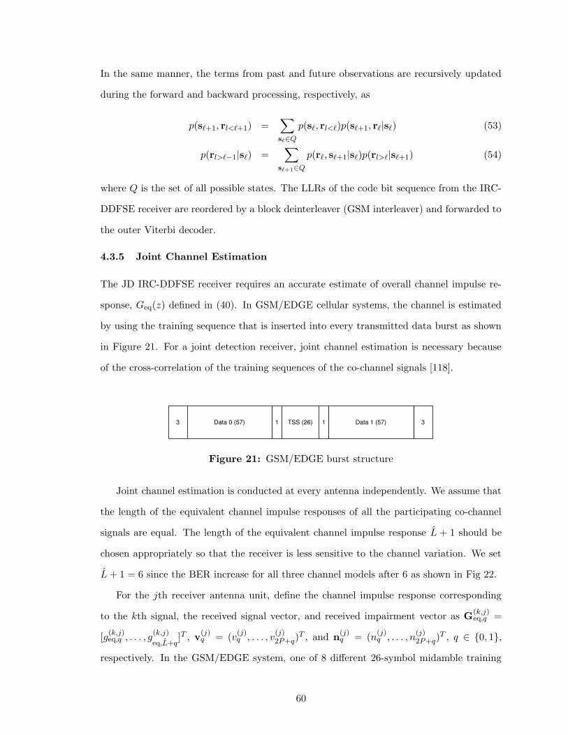
In the same manner, the terms from past and future observations are recursively updated

during the forward and backward processing, respectively, as

p(s`+1, rl<`+1) =∑

s`∈Q

p(s`, rl<`)p(s`+1, r`|s`) (53)

p(rl>`−1|s`) =∑

s`+1∈Q

p(r`, s`+1|s`)p(rl>`|s`+1) (54)

where Q is the set of all possible states. The LLRs of the code bit sequence from the IRC-

DDFSE receiver are reordered by a block deinterleaver (GSM interleaver) and forwarded to

the outer Viterbi decoder.

4.3.5 Joint Channel Estimation

The JD IRC-DDFSE receiver requires an accurate estimate of overall channel impulse re-

sponse, Geq(z) defined in (40). In GSM/EDGE cellular systems, the channel is estimated

by using the training sequence that is inserted into every transmitted data burst as shown

in Figure 21. For a joint detection receiver, joint channel estimation is necessary because

of the cross-correlation of the training sequences of the co-channel signals [118].

3 3 TSS (26) Data 0 (57) Data 1 (57) 1 1

Figure 21: GSM/EDGE burst structure

Joint channel estimation is conducted at every antenna independently. We assume that

the length of the equivalent channel impulse responses of all the participating co-channel

signals are equal. The length of the equivalent channel impulse response L + 1 should be

chosen appropriately so that the receiver is less sensitive to the channel variation. We set

L + 1 = 6 since the BER increase for all three channel models after 6 as shown in Fig 22.

For the jth receiver antenna unit, define the channel impulse response corresponding

to the kth signal, the received signal vector, and received impairment vector as G(k,j)eq,q =

[g(k,j)eq,q , . . . , g

(k,j)

eq,L+q]T , v

(j)q = (v

(j)q , . . . , v

(j)2P+q)

T , and n(j)q = (n

(j)q , . . . , n

(j)2P+q)

T , q ∈ {0, 1},

respectively. In the GSM/EDGE system, one of 8 different 26-symbol midamble training

60

symbol sequences (TSS) are inserted into each burst. For the co-channel signals with D-

symbol interval delay offset and equivalent channels of length L+1 = 6, 24−D TSS symbols

and 2(P + 1 −D) = 48 − 2D, T/2-spaced, received signal vectors are used to insure that

the known training sequences are involved in the channel estimation process.

The received samples during the training sequence at jth antenna are

v(j)q = XG(j)

eq,q + n(j)q , q = 0, 1 (55)

where G(j)eq,q = (G

(1,j)eq,q

T, . . . ,G

(N,j)eq,q

T)T is a joint channel impulse response vector, and X =

(X(1), . . . ,X(N)) is the transmitted training sequence matrix with elements

X(k) =

x(k)0 . . . x

(k)

−(L−1)/2

x(k)1 . . . x

(k)

−(L−1)/2+1...

. . ....

x(k)P . . . x

(k)

−(L−1)/2+P

. (56)

Under our time independence assumption, n(j)q , q ∈ {0, 1}, is a white Gaussian noise

vector, and the least squares solution to (55) is [75]

G(j)eq,LS,q = (XHX)−1XHv(j)

q , q = 0, 1 . (57)

4.4 Imbalanced CIRs at Antenna Branches

In general, the received CIRs are assumed equal at all antenna branches. However, the

crowded high-rise buildings and narrow streets fertilize the construction of virtual waveg-

uides for radio wave propagation in urban cities. In those radio propagation environ-

ments, average power of received signals at antenna branches may not equal. Mallik

et al ’s study shows that the imbalance of Gaussian noise across antenna branches de-

grades the performance of equal gain combining (EGC) in correlated Rayleigh faded chan-

nels [103]. Also, another study shows that optimal and selective combining receivers with

linear/nonlinear equalizer achieves minimum BER when all antenna branches have an equal

received SNRs [99].

61

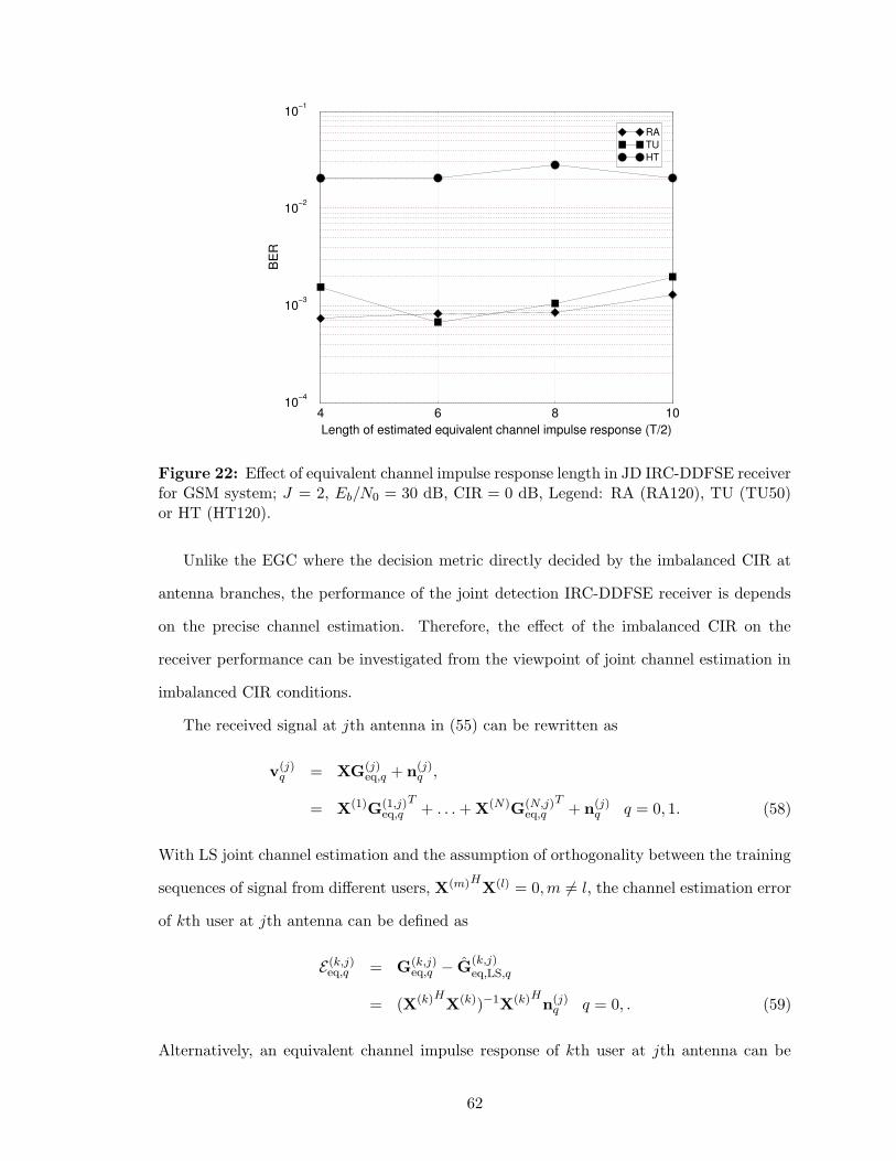
4 6 8 10Length of estimated equivalent channel impulse response (T/2)

10−4

10−3

10−2

10−1

BE

R

RATUHT

Figure 22: Effect of equivalent channel impulse response length in JD IRC-DDFSE receiverfor GSM system; J = 2, Eb/N0 = 30 dB, CIR = 0 dB, Legend: RA (RA120), TU (TU50)or HT (HT120).

Unlike the EGC where the decision metric directly decided by the imbalanced CIR at

antenna branches, the performance of the joint detection IRC-DDFSE receiver is depends

on the precise channel estimation. Therefore, the effect of the imbalanced CIR on the

receiver performance can be investigated from the viewpoint of joint channel estimation in

imbalanced CIR conditions.

The received signal at jth antenna in (55) can be rewritten as

v(j)q = XG(j)

eq,q + n(j)q ,

= X(1)G(1,j)eq,q

T+ . . . + X(N)G(N,j)

eq,q

T+ n(j)

q q = 0, 1. (58)

With LS joint channel estimation and the assumption of orthogonality between the training

sequences of signal from different users, X(m)HX(l) = 0, m 6= l, the channel estimation error

of kth user at jth antenna can be defined as

E(k,j)eq,q = G(k,j)

eq,q − G(k,j)eq,LS,q

= (X(k)HX(k))−1X(k)Hn(j)q q = 0, . (59)

Alternatively, an equivalent channel impulse response of kth user at jth antenna can be

62

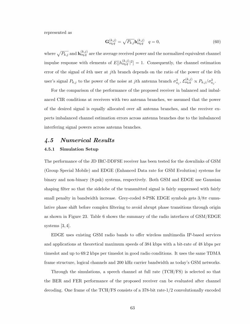
represented as

G(k,j)eq,q =

√

Pk,jh(k,j)eq,q q = 0, (60)

where√

Pk,j and h(k,j)eq,q are the average received power and the normalized equivalent channel

impulse response with elements of E[|h(k,j)eq,q |2] = 1. Consequently, the channel estimation

error of the signal of kth user at jth branch depends on the ratio of the power of the kth

user’s signal Pk,j to the power of the noise at jth antenna branch σ2nj

, E(k,j)eq,q ∝ Pk,j/σ

2nj

.

For the comparison of the performance of the proposed receiver in balanced and imbal-

anced CIR conditions at receivers with two antenna branches, we assumed that the power

of the desired signal is equally allocated over all antenna branches, and the receiver ex-

pects imbalanced channel estimation errors across antenna branches due to the imbalanced

interfering signal powers across antenna branches.

4.5 Numerical Results

4.5.1 Simulation Setup

The performance of the JD IRC-DDFSE receiver has been tested for the downlinks of GSM

(Group Special Mobile) and EDGE (Enhanced Data rate for GSM Evolution) systems for

binary and non-binary (8-psk) systems, respectively. Both GSM and EDGE use Gaussian

shaping filter so that the sidelobe of the transmitted signal is fairly suppressed with fairly

small penalty in bandwidth increase. Grey-coded 8-PSK EDGE symbols gets 3/8π cumu-

lative phase shift before complex filtering to avoid abrupt phase transitions through origin

as shown in Figure 23. Table 6 shows the summary of the radio interfaces of GSM/EDGE

systems [3, 4].

EDGE uses existing GSM radio bands to offer wireless multimedia IP-based services

and applications at theoretical maximum speeds of 384 kbps with a bit-rate of 48 kbps per

timeslot and up to 69.2 kbps per timeslot in good radio conditions. It uses the same TDMA

frame structure, logical channels and 200 kHz carrier bandwidth as today’s GSM networks.

Through the simulations, a speech channel at full rate (TCH/FS) is selected so that

the BER and FER performance of the proposed receiver can be evaluated after channel

decoding. One frame of the TCH/FS consists of a 378-bit rate-1/2 convolutionally encoded

63

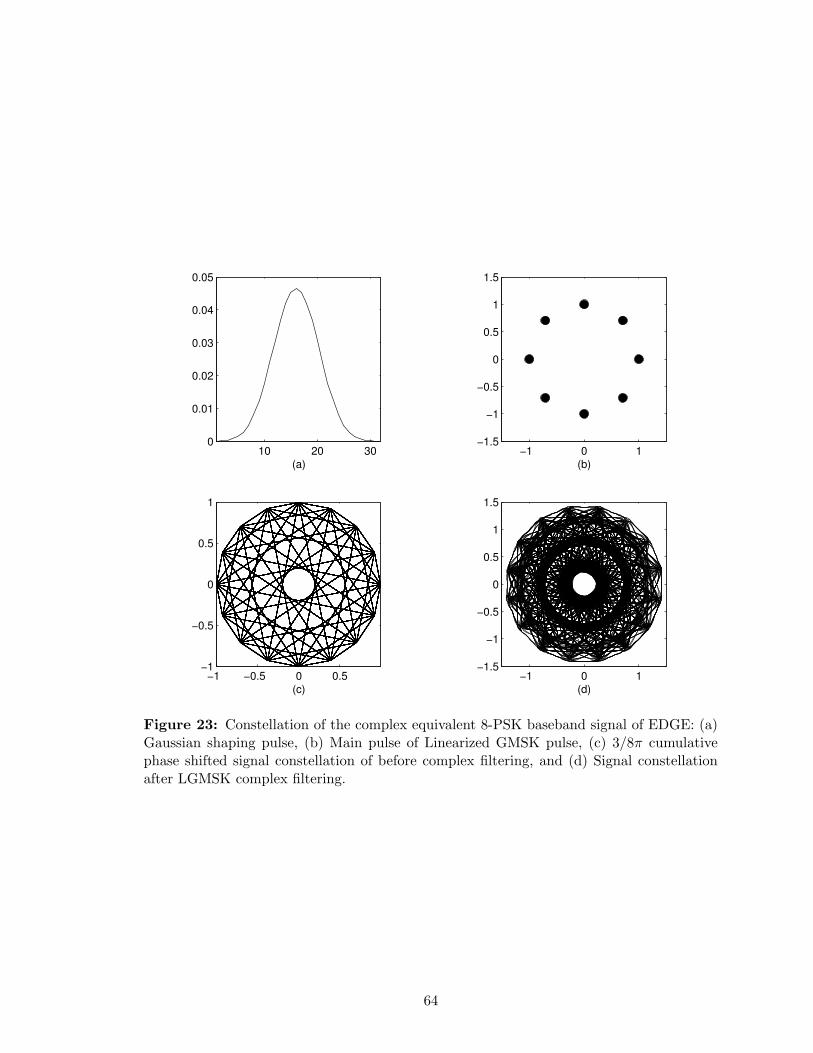
10 20 300

0.01

0.02

0.03

0.04

0.05

(a)−1 0 1

−1.5

−1

−0.5

0

0.5

1

1.5

(b)

−1 −0.5 0 0.5−1

−0.5

0

0.5

1

(c)−1 0 1

−1.5

−1

−0.5

0

0.5

1

1.5

(d)

Figure 23: Constellation of the complex equivalent 8-PSK baseband signal of EDGE: (a)Gaussian shaping pulse, (b) Main pulse of Linearized GMSK pulse, (c) 3/8π cumulativephase shifted signal constellation of before complex filtering, and (d) Signal constellationafter LGMSK complex filtering.

64

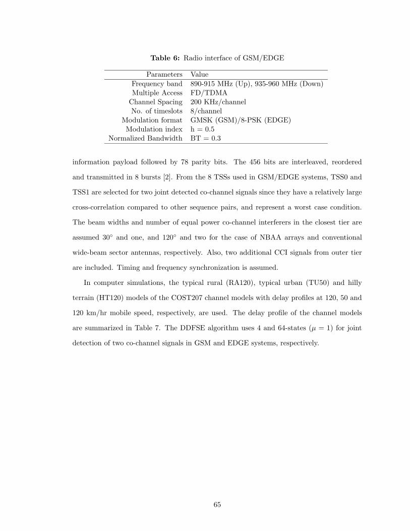
Table 6: Radio interface of GSM/EDGE

Parameters Value

Frequency band 890-915 MHz (Up), 935-960 MHz (Down)Multiple Access FD/TDMA

Channel Spacing 200 KHz/channelNo. of timeslots 8/channel

Modulation format GMSK (GSM)/8-PSK (EDGE)Modulation index h = 0.5

Normalized Bandwidth BT = 0.3

information payload followed by 78 parity bits. The 456 bits are interleaved, reordered

and transmitted in 8 bursts [2]. From the 8 TSSs used in GSM/EDGE systems, TSS0 and

TSS1 are selected for two joint detected co-channel signals since they have a relatively large

cross-correlation compared to other sequence pairs, and represent a worst case condition.

The beam widths and number of equal power co-channel interferers in the closest tier are

assumed 30◦ and one, and 120◦ and two for the case of NBAA arrays and conventional

wide-beam sector antennas, respectively. Also, two additional CCI signals from outer tier

are included. Timing and frequency synchronization is assumed.

In computer simulations, the typical rural (RA120), typical urban (TU50) and hilly

terrain (HT120) models of the COST207 channel models with delay profiles at 120, 50 and

120 km/hr mobile speed, respectively, are used. The delay profile of the channel models

are summarized in Table 7. The DDFSE algorithm uses 4 and 64-states (µ = 1) for joint

detection of two co-channel signals in GSM and EDGE systems, respectively.

65

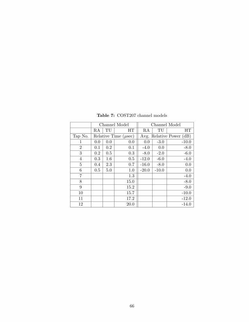
Table 7: COST207 channel models

Channel Model Channel Model

RA TU HT RA TU HT

Tap No. Relative Time (µsec) Avg. Relative Power (dB)

1 0.0 0.0 0.0 0.0 -3.0 -10.0

2 0.1 0.2 0.1 -4.0 0.0 -8.0

3 0.2 0.5 0.3 -8.0 -2.0 -6.0

4 0.3 1.6 0.5 -12.0 -6.0 -4.0

5 0.4 2.3 0.7 -16.0 -8.0 0.0

6 0.5 5.0 1.0 -20.0 -10.0 0.0

7 1.3 -4.0

8 15.0 -8.0

9 15.2 -9.0

10 15.7 -10.0

11 17.2 -12.0

12 20.0 -14.0

66

4.5.2 BER and FER Performance

Figure 24 compares the BER performance of the proposed receiver to a conventional single

user detection receiver with an NBAA array configuration. A CIR gain of approximately 10

to 15 and 1 to 3 dB is achieved over the conventional receiver for GSM and EDGE systems,

respectively, at a decoded BER of 10−2. Note that the joint detection structure achieves

higher gain in a low CIR range than in a high CIR range. In highly dispersive channels

(TU50,HT120), only a fraction of signal energy is considered in the channel taps used in

DDFSE function. Therefore, the detection can be easily impaired by a small amount of

noise-plus-interference and the diversity gain fades especially when the channel taps are in

deep fade.

Figure 25 illustrates that the joint detection receiver is highly effective when it have

NBAA preprocessor. The increased number of interfering signals receiving at conventional

sector antenna configuration fairly degrades the BER performance of the proposed receiver.

Also, by its nature, the narrow beam pattern of NBAA reduces the length of channel impulse

response of the desired signal and escalates the gain from DDFSE structure even in highly

dispersive channel conditions.

For services that use block-by-block CRC-check and retransmission schemes, the FER is

widely accepted as a performance measurement since most QoS specifications are in terms

of the FER. At 10% FER criterion, the joint detection technique yields 2 to 12 and 1 to

6 dB CIR gains over a conventional receiver for GSM and EDGE, respectively, as shown

in Figure 26. The FER of a communication link depends on the received BER and the

channel coding technique employed. Therefore, the achieved FER will be lowered in case

of data packets normally protected by stronger channel coding than speech packets such as

TCH/FS.

In synchronized networks, the delay offset is expected to be smaller than 3 symbol

durations. Figure 27 illustrates that delay offset between the two co-channel signal bursts

which are jointly detected has a relatively minor effect on BER performance in synchronized

networks. Fractionally spaced structure of the receiver as well as the joint channel estimation

diminishes the impairments from the delay offset on BER performance.

67

4.5.3 Performance Variation with Imbalanced CIR

For the imbalanced CIR conditions, the simulation results show that the performance of

the receiver is optimal in balanced CIR conditions, and the BER performance gap between

balanced and imbalanced conditions tends to increase as the average received CIR increases

as shown in Figure 28. In contrast, the single detection receiver is virtually unaffected

by the imbalanced conditions as shown in Figure 29. The performance loss of the joint

detection receiver from imbalanced CIR conditions can be explained by the nature of joint

channel estimation. In general, the channel estimation error of the interfering signal in joint

detection receivers results in error floor in the BER of the desired signal in high CIR region.

For the proposed receiver in imbalanced CIR conditions, an interfering signal arriving at

one antenna branch experiences higher CIR and suffers larger channel estimation error

than the other one arriving at antenna branch of lower CIR. This large error contributes to

the decision metric, especially in high CIR regions. The desired signal experiences similar

asymmetric channel estimation errors in low CIR region. However, the outcome of an equal

amount of channel estimation error in a low BER range is more critical than that in a high

BER range.

68

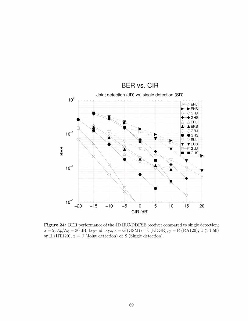
−20 −15 −10 −5 0 5 10 15 20CIR (dB)

10−3

10−2

10−1

100

BE

R

BER vs. CIRJoint detection (JD) vs. single detection (SD)

EHJEHSGHJGHSERJERSGRJGRSEUJEUSGUJGUS

Figure 24: BER performance of the JD IRC-DDFSE receiver compared to single detection;J = 2, Eb/N0 = 30 dB, Legend: xyz, x = G (GSM) or E (EDGE), y = R (RA120), U (TU50)or H (HT120), z = J (Joint detection) or S (Single detection).

69

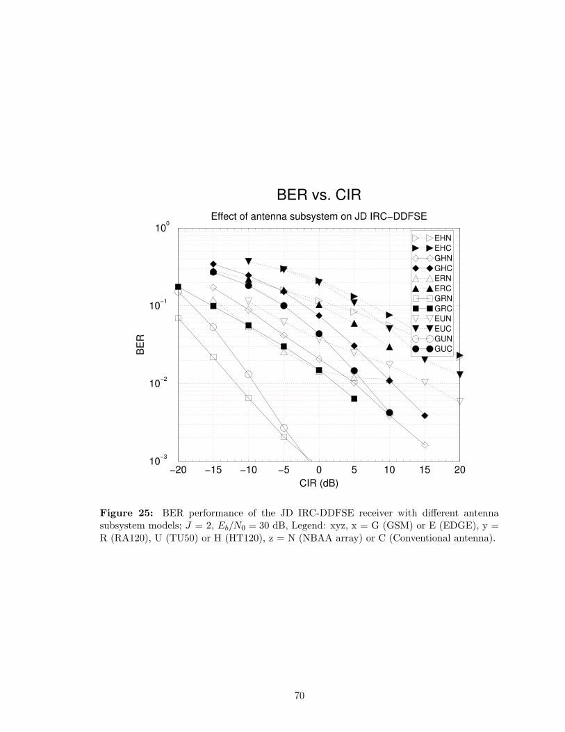
−20 −15 −10 −5 0 5 10 15 20CIR (dB)

10−3

10−2

10−1

100

BE

R

BER vs. CIREffect of antenna subsystem on JD IRC−DDFSE

EHNEHCGHNGHCERNERCGRNGRCEUNEUCGUNGUC

Figure 25: BER performance of the JD IRC-DDFSE receiver with different antennasubsystem models; J = 2, Eb/N0 = 30 dB, Legend: xyz, x = G (GSM) or E (EDGE), y =R (RA120), U (TU50) or H (HT120), z = N (NBAA array) or C (Conventional antenna).

70

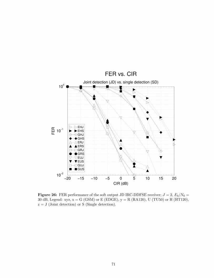
−20 −15 −10 −5 0 5 10 15 20CIR (dB)

10−2

10−1

100

FER

FER vs. CIRJoint detection (JD) vs. single detection (SD)

EHJEHSGHJGHSERJERSGRJGRSEUJEUSGUJGUS

Figure 26: FER performance of the soft output JD IRC-DDFSE receiver; J = 2, Eb/N0 =30 dB, Legend: xyz, x = G (GSM) or E (EDGE), y = R (RA120), U (TU50) or H (HT120),z = J (Joint detection) or S (Single detection).

71

−2 −1.5 −1 −0.5 0 0.5 1 1.5 2Delay offset (T)

10−4

10−3

10−2

10−1

BE

R

Delay OffsetEffect of timing delay offset between co−channel signals

RATUHT

Figure 27: Effect of the timing offset between two jointly detected co-channel signals forGSM system; J = 2, Eb/N0 = 30 dB, CIR = 0 dB, Legend: RA (RA120), TU (TU50) orHT (HT120).

72

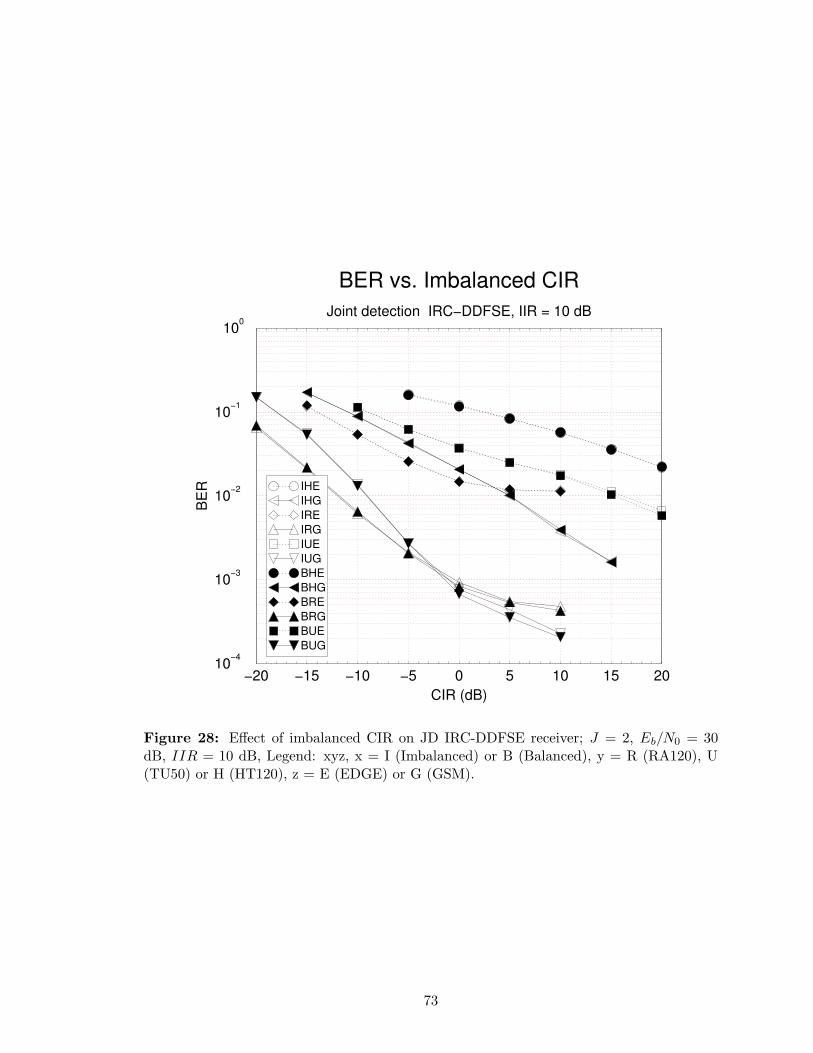
−20 −15 −10 −5 0 5 10 15 20CIR (dB)

10−4

10−3

10−2

10−1

100

BE

R

BER vs. Imbalanced CIRJoint detection IRC−DDFSE, IIR = 10 dB

IHEIHGIREIRGIUEIUGBHEBHGBREBRGBUEBUG

Figure 28: Effect of imbalanced CIR on JD IRC-DDFSE receiver; J = 2, Eb/N0 = 30dB, IIR = 10 dB, Legend: xyz, x = I (Imbalanced) or B (Balanced), y = R (RA120), U(TU50) or H (HT120), z = E (EDGE) or G (GSM).

73

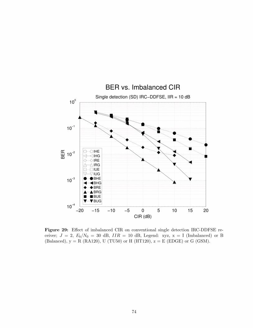
−20 −15 −10 −5 0 5 10 15 20CIR (dB)

10−4

10−3

10−2

10−1

100

BE

R

BER vs. Imbalanced CIRSingle detection (SD) IRC−DDFSE, IIR = 10 dB

IHEIHGIREIRGIUEIUGBHEBHGBREBRGBUEBUG

Figure 29: Effect of imbalanced CIR on conventional single detection IRC-DDFSE re-ceiver; J = 2, Eb/N0 = 30 dB, IIR = 10 dB, Legend: xyz, x = I (Imbalanced) or B(Balanced), y = R (RA120), U (TU50) or H (HT120), z = E (EDGE) or G (GSM).

74

CHAPTER V

INTERFERENCE MITIGATION IN MIMO SYSTEMS BY

SUBSET ANTENNA TRANSMISSION

5.1 Introduction

The capacity of a multiple-input multiple-output (MIMO) system depends on the number

of transmit/receive antennas, the correlation between the channel coefficients of individual

paths, and the method for allocating the power over the transmit antennas [147]. If channel

state information (CSI) is available at the transmitter, power allocation by a water-filling

algorithm is known to optimize capacity for AWGN channels. Likewise, if CSI is not avail-

able, equal power distribution is optimum for AWGN channels. However, if co-channel

interference (CCI) is present, these techniques no longer optimize capacity.

Previous studies on the techniques of power allocation in MIMO systems have focused on

the characteristics of the propagation channel matrix. In [106], a game theoretic approach

is introduced to verify the optimality of water-filing and equal-power methods in with-

and without-CSI at transmitter cases, respectively. On the other hand, the observation

of non-uniform eignemodes and associated eigenvalues of channel matrices prompted other

approaches that use non-equal power distribution over selected subset of transmit anten-

nas [22,111]. To maximize the information channel capacity, adaptive modulation on eigen-

modes and adaptive bit loading techniques with minimum mean square error (MMSE) crite-

rion are introduced with non-uniform power loading [61,74]. Also, various transmit/receive

antenna selection techniques for ZF and MMSE receivers have been proposed to maximize

received SINR and channel capacity by using decision metric computed from the channel

matrix [57,69,70].

CCI by nature is colored noise with non-zero off-diagonal terms in its covariance matrix.

These correlations spoil the optimality of water-filing method when CSI of CCI is not

75

available at transmitters [48, 126]. The recent work by Blum [26] has taken an initial step

on the problem of power allocation in the presence of CCI, by switching between two power

allocation strategies; i) transmitting equal-power over all antennas, and ii) transmitting

all-power over one antenna. Another approach uses MIMO multiuser detection to process

the co-channel signals [64, 153]. However, Blum’s approach suffers from a large capacity

loss as the number of transmit antennas increases, while the approach of Goldsmith et al.

is only feasible when full CSI of all co-channel signals is available [64].

This study investigates the performance of an adaptive practical power distribution

scheme by using subset antenna transmission (SAT) for MIMO systems. The introduction of

the SAT scheme is motivated by the observation of reduced eigenmodes in severely perturbed

MIMO channels [120]. In the SAT scheme, the transmit power is distributed equally across

subset of the transmit antennas. The subset is determined from criteria generated from

CSI of the desired signal, while CSI of the CCI is not needed. This simplicity makes the

SAT scheme beneficial in most practical systems where the CSI of CCI is not available.

The capacity gain from the increased transmit power per antenna with SAT is evaluated

by computer simulations with V-BLAST systems. Also, we investigated the performance

of the space-time diversity coding (STDC) scheme in terms of interference mitigation for

comparison. While the STDC exploits the gain from spatial and temporal diversity at the

cost of increased redundancy, the SAT scheme use only the property of spatial multiplexing

of MIMO systems.

The remainder of this chapter is organized as follows: Section 5.2 provides system and

channel models of MIMO systems in the presence of CCI and noise. Section 5.3 intro-

duces phenomena of reduced eigenmodes in terms of the condition number and the effective

eigenmodes of the channel matrix. In Section 5.4, the capacity gain from adaptive power

allocation with SAT is characterized. Section 5.5 presents an application of the SAT scheme

to a 4×4 V-BLAST MIMO system. Section 5.6 probes the capability of a space-time diver-

sity coding scheme in terms of CCI mitigation in MIMO systems. Section 5.7 discusses the

performance of the proposed power allocation schemes evaluated on 4× 4 and 2× 2 MIMO

systems by computer simulations.

76

5.2 Channel Capacity with Equivalent Channel Matrix

5.2.1 System and Channel Models

The system under consideration has a single-user link of interest affected by CCI from

another user. The user of interest and interfering user have M transmit and N receive

antennas, respectively. In a flat faded MIMO system, the received signal vector yN×1 is

y =√

PTHs +√

PIHIsI + w

= Hs + n (61)

where HN×M , sM×1 and PT are the MIMO channel matrix and transmitted signal vector

and power of the user of interest, respectively, HI N×M , sI and PI are the channel matrix,

transmit signal, and power of the interfering signal, respectively, and wN×1 is the thermal

noise with covariance matrix E{wwH} = σ2IN where H denotes conjugate transpose. The

vector nN×1 is the interference-plus-noise vector.

The channel matrices H and HI are mutually independent, and assumed to be quasi-

static. The elements in H and HI are independent identically distributed (i.i.d.) zero-mean

complex Gaussian random variables with unit variance. Also, the signal of the user of

interest, interferer’s signal and the thermal noise, s, sI , and w, respectively, are mutually

independent. The spatial covariance matrix of interference-plus-noise is Kn = E{nnH}.

The covariance matrix of the user of interest is Φ = E{ssH}. The covariance matrix of the

received signal component of the user of interest is Kd = HΦHH .

77

5.2.2 Mutual Information

Assuming the interference has a Gaussian distribution, the optimal input distribution of s

is Gaussian [34,134]. The mutual information between the channel input s and output y is

I = log2 det(Kd + Kn)− log2 det(Kn)

= log2 det(Kd(Kn)−1 + IN )

= log2 det(HΦHH(Kn)−1 + IN )

= log2 det(((Kn)−1/2H)Φ((Kn)−1/2H)H + IN )

= log2 det(((Kn)−1/2H)H((Kn)−1/2H)Φ + IM )

= log2 det(HHHΦ + IM ) (62)

where the determinant identity det(AB + I) = det(BA + I) is used in the fifth equality.

Eq. (62) represents the mutual information of the equivalent channel H = (Kn)−1/2H.

5.2.3 CSI Available at Transmitter

When CSI of the equivalent channel H is available at the transmitter, the channel ca-

pacity is achieved by a water-filling solution, where Φ is chosen to maximize the mutual

information subject to the power constraint tr(Φ) ≤ PT. Since HHH is Hermitian, it can

be diagonalized, i.e., HHH = UΛUH , with unitary matrix U and non-negative diagonal

matrix Λ = diag(λ1, . . . , λM ). The mutual information in (62) can be rewritten as

I = log2 det(UΛUHΦ + IM )

= log2 det(Λ1/2UHΦUΛ1/2 + IM ). (63)

Since UHΦU is positive definite if and only if Φ is, and tr(UHΦU) = tr(Φ), the channel

capacity is achieved when UHΦU is diagonal

UHΦU = diag(p1, . . . , pM ). (64)

The optimal diagonal entries of UHΦU can be found via the water-filling process

pi = (µ− λ−1i )+, i = 1, . . . , M (65)

78

where µ is chosen to satisfy the sum constraint∑

i pi = PT , and (·)+ is zero when the

argument is negative. The corresponding channel capacity is

C = max{pi}I =

M∑

i=1

log2(1 + piλi). (66)

5.2.4 CSI not Available at Transmitter

If CSI is not available at the transmitter, the optimal transmit covariance is Φ = (PT /M)IM ,

and the channel capacity is

C = log2 det

(

PT

MHHH + IN

)

. (67)

In a noise-limited or white-interference conditions, Kn = σ2I and the capacity is

C = log2 det

(

PT

σ2MHHH + IN

)

. (68)

5.3 Eigenmodes, Condition Number and Power Allocation

5.3.1 Eigenmodes of Channel Matrix

The channel matrix H∈N×M linking the transmitter and the receiver can be represented in

terms of a singular value decomposition (SVD): H = UΛVH , where U∈N×N and V∈M×M

are complex unitary matrices, and Λ∈N×M = diag(√

λ1, . . . ,√

λr, 0, . . . , 0) is a diagonal

matrix, where the nonzero diagonal elements are the square roots of the eigenvalues of the

channel covariance matrix K = HHH . The number of nonzero eigenvalues is equal to

the rank of the covariance matrix, r ≤ min{M, N}. With orthogonal SVD, the N ×M

MIMO channel can be decomposed into r independent single-input single-output (SISO)

channels, called eigenmodes or eigenchannels, where the received signal on the ith channel is

yi =√

λisi+ni. Each eigenvalue represents the amount of power that is transferred through

the channel into the direction coordinated by the corresponding eigenvector. Of course the

eigenvalues are unequal for a random realization of H. When a subset of eigenvalues of a

matrix are negligible in magnitude compared to the others, the matrix transformation can be

well approximated by the set of eigenvalues of significant magnitudes and the corresponding

eigenvectors [105]. In such a case, the condition number of the channel matrix is a useful

indicator of unequal eigenmodes.

79

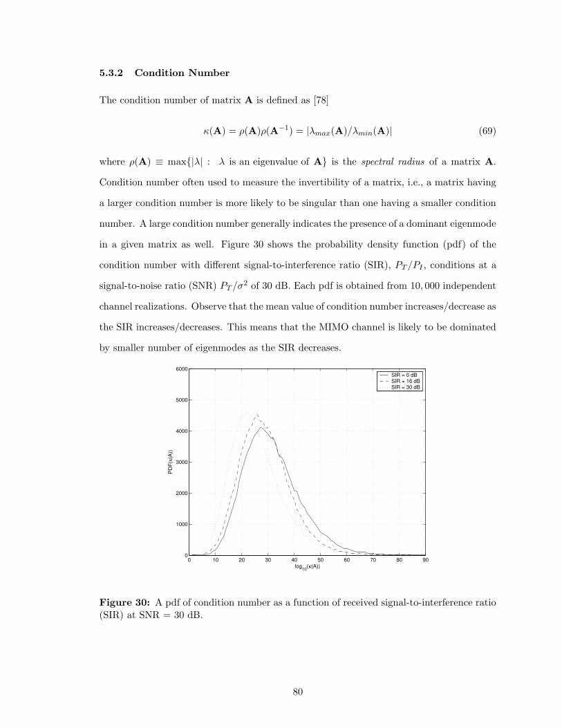
5.3.2 Condition Number

The condition number of matrix A is defined as [78]

κ(A) = ρ(A)ρ(A−1) = |λmax(A)/λmin(A)| (69)

where ρ(A) ≡ max{|λ| : λ is an eigenvalue of A} is the spectral radius of a matrix A.

Condition number often used to measure the invertibility of a matrix, i.e., a matrix having

a larger condition number is more likely to be singular than one having a smaller condition

number. A large condition number generally indicates the presence of a dominant eigenmode

in a given matrix as well. Figure 30 shows the probability density function (pdf) of the

condition number with different signal-to-interference ratio (SIR), PT /PI , conditions at a

signal-to-noise ratio (SNR) PT /σ2 of 30 dB. Each pdf is obtained from 10, 000 independent

channel realizations. Observe that the mean value of condition number increases/decrease as

the SIR increases/decreases. This means that the MIMO channel is likely to be dominated

by smaller number of eigenmodes as the SIR decreases.

0 10 20 30 40 50 60 70 80 900

1000

2000

3000

4000

5000

6000

log10

(κ(A))

PD

F(κ(

A))

SIR = 0 dBSIR = 16 dBSIR = 30 dB

Figure 30: A pdf of condition number as a function of received signal-to-interference ratio(SIR) at SNR = 30 dB.

80

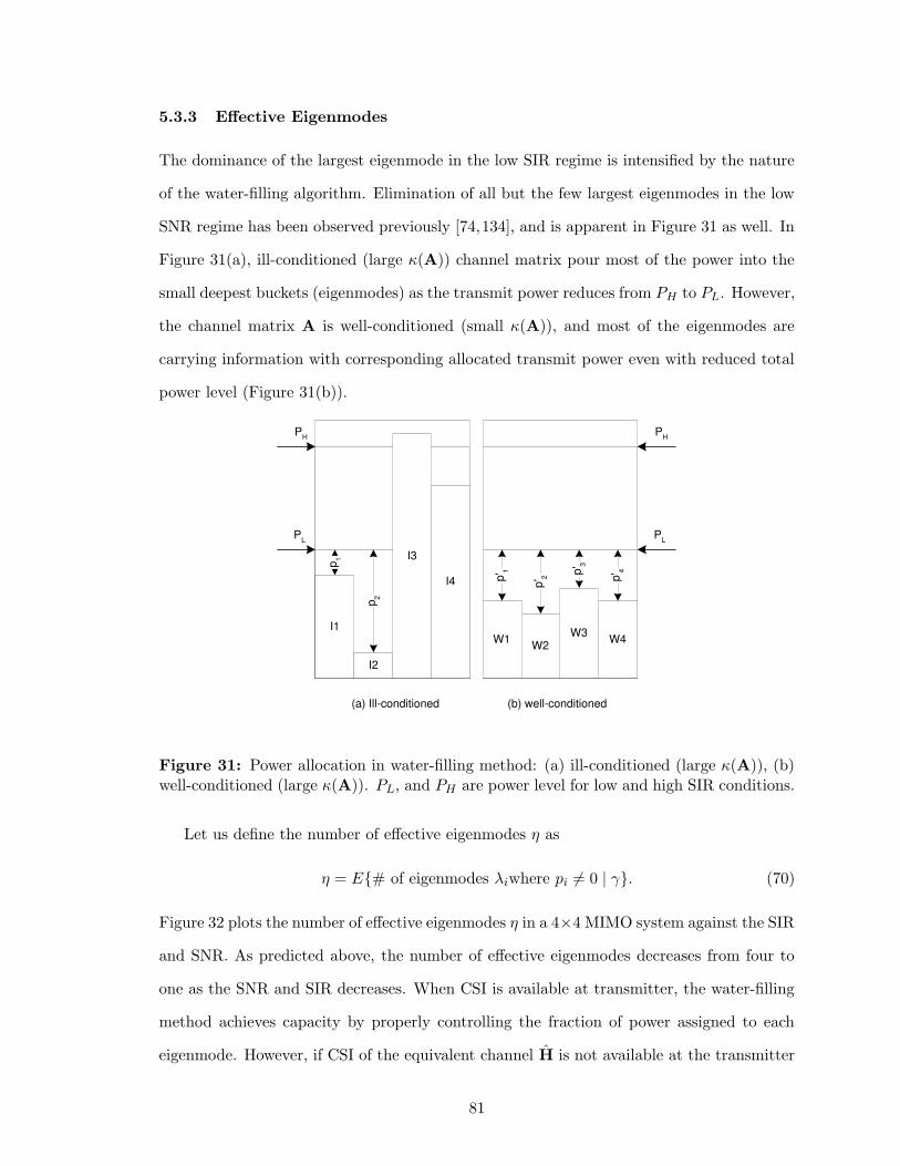
5.3.3 Effective Eigenmodes

The dominance of the largest eigenmode in the low SIR regime is intensified by the nature

of the water-filling algorithm. Elimination of all but the few largest eigenmodes in the low

SNR regime has been observed previously [74,134], and is apparent in Figure 31 as well. In

Figure 31(a), ill-conditioned (large κ(A)) channel matrix pour most of the power into the

small deepest buckets (eigenmodes) as the transmit power reduces from PH to PL. However,

the channel matrix A is well-conditioned (small κ(A)), and most of the eigenmodes are

carrying information with corresponding allocated transmit power even with reduced total

power level (Figure 31(b)).

P H

P L

I1

I4

I2

I3

p 2

p 1

W1 W4 W3 W2

p' 1

p' 2 p'

3

p' 4

(a) Ill-conditioned (b) well-conditioned

P H

P L

Figure 31: Power allocation in water-filling method: (a) ill-conditioned (large κ(A)), (b)well-conditioned (large κ(A)). PL, and PH are power level for low and high SIR conditions.

Let us define the number of effective eigenmodes η as

η = E{# of eigenmodes λiwhere pi 6= 0 | γ}. (70)

Figure 32 plots the number of effective eigenmodes η in a 4×4 MIMO system against the SIR

and SNR. As predicted above, the number of effective eigenmodes decreases from four to

one as the SNR and SIR decreases. When CSI is available at transmitter, the water-filling

method achieves capacity by properly controlling the fraction of power assigned to each

eigenmode. However, if CSI of the equivalent channel H is not available at the transmitter

81

and all transmit antennas are assigned equal power, a capacity loss arises from the unequal

eigenmodes. Therefore, we need to improve the equal-power algorithm in this case.

05

1015

2025

30

−10−5

05

1015

200

0.5

1

1.5

2

2.5

3

3.5

4

SNR (dB)SIR (dB)

η

Figure 32: Average number of effective eigenmodes: Both transmitter and receiver areequipped with four antennas, M = N = 4.

5.4 Subset Antenna Transmission

Under ideal conditions where the CSI of desired and interfering signals are available at

transmitters, the water-filling method achieves capacity regardless the received SIR and the

condition number of the equivalent channel matrix H. However, in many practical systems,

CSI of interfering signal is not available at the transmitter. In such cases, an equal power

distribution across the transmit antennas is the most feasible power allocation strategy. The

SAT method uses an equal-power distribution as well, but only uses a subset containing M

of the M antennas.

82

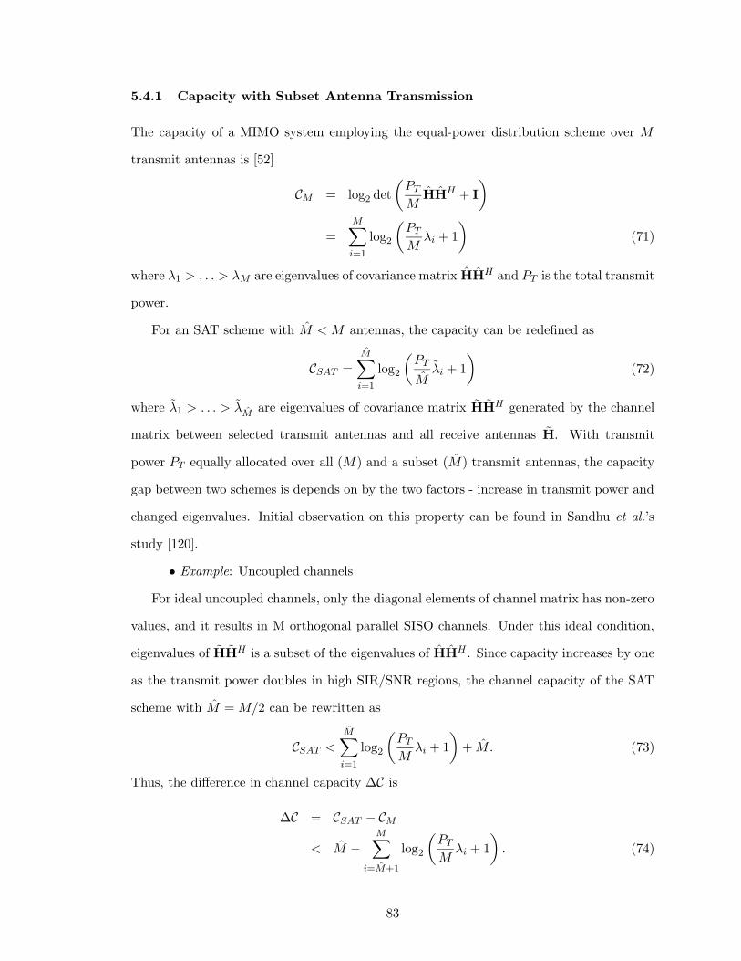
5.4.1 Capacity with Subset Antenna Transmission

The capacity of a MIMO system employing the equal-power distribution scheme over M

transmit antennas is [52]

CM = log2 det

(

PT

MHHH + I

)

=M∑

i=1

log2

(

PT

Mλi + 1

)

(71)

where λ1 > . . . > λM are eigenvalues of covariance matrix HHH and PT is the total transmit

power.

For an SAT scheme with M < M antennas, the capacity can be redefined as

CSAT =M∑

i=1

log2

(

PT

Mλi + 1

)

(72)

where λ1 > . . . > λM are eigenvalues of covariance matrix HHH generated by the channel

matrix between selected transmit antennas and all receive antennas H. With transmit

power PT equally allocated over all (M) and a subset (M) transmit antennas, the capacity

gap between two schemes is depends on by the two factors - increase in transmit power and

changed eigenvalues. Initial observation on this property can be found in Sandhu et al.’s

study [120].

• Example: Uncoupled channels

For ideal uncoupled channels, only the diagonal elements of channel matrix has non-zero

values, and it results in M orthogonal parallel SISO channels. Under this ideal condition,

eigenvalues of HHH is a subset of the eigenvalues of HHH . Since capacity increases by one

as the transmit power doubles in high SIR/SNR regions, the channel capacity of the SAT

scheme with M = M/2 can be rewritten as

CSAT <

M∑

i=1

log2

(

PT

Mλi + 1

)

+ M. (73)

Thus, the difference in channel capacity ∆C is

∆C = CSAT − CM

< M −M∑

i=M+1

log2

(

PT

Mλi + 1

)

. (74)

83

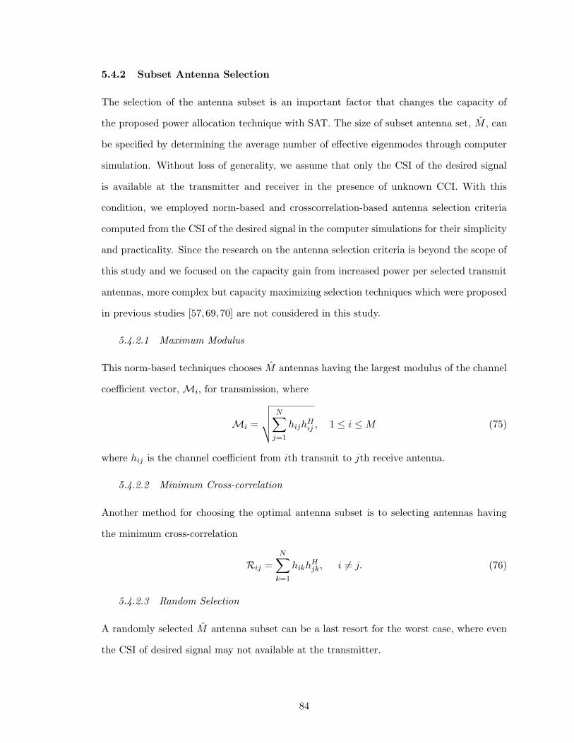
5.4.2 Subset Antenna Selection

The selection of the antenna subset is an important factor that changes the capacity of

the proposed power allocation technique with SAT. The size of subset antenna set, M , can

be specified by determining the average number of effective eigenmodes through computer

simulation. Without loss of generality, we assume that only the CSI of the desired signal

is available at the transmitter and receiver in the presence of unknown CCI. With this

condition, we employed norm-based and crosscorrelation-based antenna selection criteria

computed from the CSI of the desired signal in the computer simulations for their simplicity

and practicality. Since the research on the antenna selection criteria is beyond the scope of

this study and we focused on the capacity gain from increased power per selected transmit

antennas, more complex but capacity maximizing selection techniques which were proposed

in previous studies [57, 69,70] are not considered in this study.

5.4.2.1 Maximum Modulus

This norm-based techniques chooses M antennas having the largest modulus of the channel

coefficient vector,Mi, for transmission, where

Mi =

√

√

√

√

N∑

j=1

hijhHij , 1 ≤ i ≤M (75)

where hij is the channel coefficient from ith transmit to jth receive antenna.

5.4.2.2 Minimum Cross-correlation

Another method for choosing the optimal antenna subset is to selecting antennas having

the minimum cross-correlation

Rij =

N∑

k=1

hikhHjk, i 6= j. (76)

5.4.2.3 Random Selection

A randomly selected M antenna subset can be a last resort for the worst case, where even

the CSI of desired signal may not available at the transmitter.

84

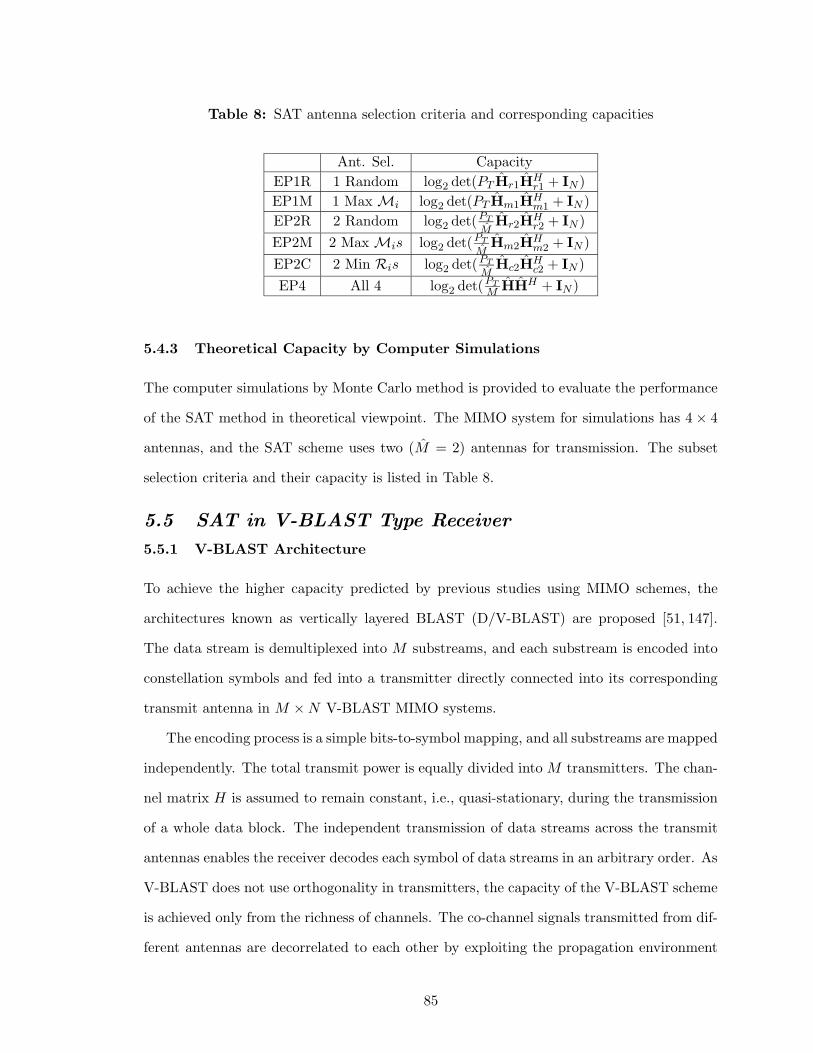
Table 8: SAT antenna selection criteria and corresponding capacities

Ant. Sel. Capacity

EP1R 1 Random log2 det(PT Hr1HHr1 + IN )

EP1M 1 Max Mi log2 det(PT Hm1HHm1 + IN )

EP2R 2 Random log2 det(PT

MHr2H

Hr2 + IN )

EP2M 2 Max Mis log2 det(PT

MHm2H

Hm2 + IN )

EP2C 2 Min Ris log2 det(PT

MHc2H

Hc2 + IN )

EP4 All 4 log2 det(PT

M HHH + IN )

5.4.3 Theoretical Capacity by Computer Simulations

The computer simulations by Monte Carlo method is provided to evaluate the performance

of the SAT method in theoretical viewpoint. The MIMO system for simulations has 4× 4

antennas, and the SAT scheme uses two (M = 2) antennas for transmission. The subset

selection criteria and their capacity is listed in Table 8.

5.5 SAT in V-BLAST Type Receiver

5.5.1 V-BLAST Architecture

To achieve the higher capacity predicted by previous studies using MIMO schemes, the

architectures known as vertically layered BLAST (D/V-BLAST) are proposed [51, 147].

The data stream is demultiplexed into M substreams, and each substream is encoded into

constellation symbols and fed into a transmitter directly connected into its corresponding

transmit antenna in M ×N V-BLAST MIMO systems.

The encoding process is a simple bits-to-symbol mapping, and all substreams are mapped

independently. The total transmit power is equally divided into M transmitters. The chan-

nel matrix H is assumed to remain constant, i.e., quasi-stationary, during the transmission

of a whole data block. The independent transmission of data streams across the transmit

antennas enables the receiver decodes each symbol of data streams in an arbitrary order. As

V-BLAST does not use orthogonality in transmitters, the capacity of the V-BLAST scheme

is achieved only from the richness of channels. The co-channel signals transmitted from dif-

ferent antennas are decorrelated to each other by exploiting the propagation environment

85

itself.

5.5.2 Decoding Process of V-BLAST

The detection process of the V-BLAST scheme estimates the transmitted symbols s given

received signal vector y and channel matrix H in

y = Hs + n. (77)

For the SAT scheme, the M elements of the transmitted symbol vector s are assumed

to be uncorrelated. The channel matrix is assumed to be known to the receiver, and to be

full rank. The decision process involves linear nulling and estimated symbol cancellation.

Nulling is performed by linearly weighting the received signals so as to satisfy performance

criteria, such as MMSE and ZF. Non-linear technique of symbol cancellation brings superior

performance by subtracting out the interference from already-detected components of s, and

results in a modified received signal vector, in which fewer interferers are present.

5.5.2.1 Nulling

Denoting the ith column of H as Hi the received signal vector can be rewritten as

y = s1H1 + s2H2 + . . . + sMHM + n (78)

where si is the transmitted symbol from the ith transmit antenna. For ZF nulling, the

nulling vector wi is chosen such that

wTi Hj = δij (79)

where δ is Kronecker delta. Thus the decision statistic for the ith substream is yi = wTi y.

Then the soft or hard decision can be made on yi to estimate the transmitted symbol

si = Q(yi) (80)

where Q(·) denotes the slicing operation appropriate to the constellation in use.

86

5.5.2.2 Successive Interference Cancellation

Denoting the received vector y by y1, if the nulling vector is w1, then the decision statistic

for the estimation of the first symbol x1 is

d1 = wT1 y1. (81)

Then the interference from the estimated symbol s1 = Q(d1) on the other symbols can be

subtracted as

y2 = y1 − s1H1y1. (82)

assuming that s1 is correctly detected. The next symbols s2, . . . , sM are detected by finding

w2, . . . ,wM and subtracting the replica of the previously estimated symbols, s2H2, . . . , sMHM .

The performance of the V-BLAST scheme depends on the error propagation from incor-

rect symbol decision from the early stages. Consequently, an optimal detection ordering is

required to minimize the detection errors in the subsequent detection stages.

5.5.2.3 Detection Ordering

A simple but effective ordering is based on the postdetection SNR of each substream to

minimize the error propagation by detecting stronger symbols first. The SNR for the ith

detected symbol of vector y is given by [147]

ρi =E{|si|2}

σ2(‖ wi ‖2)(83)

where σ2 is the noise power. If all the substreams have the same expected signal and

noise power, the postdetection SNR is depends on the inverse of the weight vector of each

substream. From (79) and ‖ wTi Hi ‖2=‖ wi ‖2‖ Hi ‖2, a larger ‖ Hi ‖2 value requires a

smaller corresponding ‖ wi ‖2. Thus, the optimal detection order is in decreasing order of

the Eucldean or l2 − norm of the columns of H.

5.5.2.4 Computation of Nulling Vector

When the channel matrix H has full rank, the vector wi in (79) is unique and is the ith

row of the pseudoinverse of channel matrix H

wi =⟨

H+⟩

i(84)

87

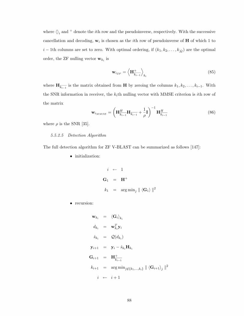
where 〈〉i and + denote the ith row and the pseudoinverse, respectively. With the successive

cancellation and decoding, wi is chosen as the ith row of pseudoinverse of H of which 1 to

i− 1th columns are set to zero. With optimal ordering, if (k1, k2, . . . , kM ) are the optimal

order, the ZF nulling vector wkiis

wiZF=⟨

H+ki−1

⟩

ki

(85)

where Hki−1is the matrix obtained from H by zeroing the columns k1, k2, . . . , ki−1. With

the SNR information in receiver, the kith nulling vector with MMSE criterion is ith row of

the matrix

wiMMSE=

(

HHki−1

Hki−1+

1

ρI

)−1

HHki−1

(86)

where ρ is the SNR [35].

5.5.2.5 Detection Algorithm

The full detection algorithm for ZF V-BLAST can be summarized as follows [147]:

• initialization:

i ← 1

G1 = H+

k1 = arg minj ‖ 〈G1〉 ‖2

• recursion:

wki= 〈Gi〉ki

dki= wT

kiyi

ski= Q(dki

)

yi+1 = yi − skiHki

Gi+1 = H+ki−1

ki+1 = arg minj /∈{k1,...,ki} ‖ 〈Gi+1〉j ‖2

i ← i + 1

88

5.5.3 Capacity in V-BLAST System Model

The capacities discussed in previous section are the limit under ideal conditions. In contrast,

real systems achieve portions of that capacity because of imperfect channel estimation. The

capacity of a real system is defined as a throughput measured with a particular system

architecture. For an example, an uncoded M-ary QAM communication system that is

employing ideal Nyquist pulses Sinc(t/Ts) at a bit rate of R = (log2M)/Ts occupies a

bandwith of W = 1/Ts and yields the throughput of log2M bps/Hz. In addition, the errors

during the transmission undermines the achievable capacity.

To measure the capacity gain achieved with the SAT method in real systems, we consider

a V-BLAST system having the same number of transmit and receive antennas as in the

theoretical case. QPSK and 16-QAM signal constellations are employed. The block error

rate (BLER) is used as a figure of merit for given system architecture [30]. The BLER can

be used in systems employing a block coding techniques. If a data block consists of NBL

sub-blocks of length LBL = L/NBL, where L is the data packet length, the BLER εBLiof

ith communication link of a MIMO system controlled by the BER εbiand the number of

bit errors Nc in each sub-block which can be corrected by the block coding technique, is

εBLi= 1−

[

Nc∑

i=0

(

LBL

i

)

(εbi)i(1− εbi

)LBL−i

]NBL

. (87)

The corresponding capacity of the link is [30]

Ci = log2 Mi(1− εBLi) (88)

where log2 Mi is the number of bits per symbol. For a MIMO system transmitting M

independent substreams of data from M transmit antennas, the total throughput of the

system is then

CT =m∑

i

Ci. (89)

5.6 Rate Adaptive Space-Time Diversity Coding for CCI

Mitigation

The SAT scheme is designed to mitigate the capacity loss from high-power interference by

redistributing the power over selected antenna subset. Likewise, the space-time diversity

89

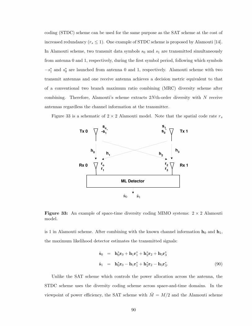
coding (STDC) scheme can be used for the same purpose as the SAT scheme at the cost of

increased redundancy (rs ≤ 1). One example of STDC scheme is proposed by Alamouti [14].

In Alamouti scheme, two transmit data symbols s0 and s1 are transmitted simultaneously

from antenna 0 and 1, respectively, during the first symbol period, following which symbols

−s∗1 and s∗0 are launched from antenna 0 and 1, respectively. Alamouti scheme with two

transmit antennas and one receive antenna achieves a decision metric equivalent to that

of a conventional two branch maximum ratio combining (MRC) diversity scheme after

combining. Therefore, Alamouti’s scheme extracts 2Nth-order diversity with N receive

antennas regardless the channel information at the transmitter.

Figure 33 is a schematic of 2 × 2 Alamouti model. Note that the spatial code rate rs

Tx 0 Tx 1 s o -s 1

* s 1 s 0

*

ML Detector

h 1

h 3 h 2

h 0

r o r 1

r 2 r 3

Rx 1 Rx 0

PSfrag replacements

s0 s1

Figure 33: An example of space-time diversity coding MIMO systems: 2 × 2 Alamoutimodel.

is 1 in Alamouti scheme. After combining with the known channel information h0 and h1,

the maximum likelihood detector estimates the transmitted signals:

s0 = h∗0r0 + h1r

∗1 + h∗

2r2 + h3r∗3

s1 = h∗0r0 − h1r

∗1 + h∗

2r2 − h3r∗3. (90)

Unlike the SAT scheme which controls the power allocation across the antenna, the

STDC scheme uses the diversity coding scheme across space-and-time domains. In the

viewpoint of power efficiency, the SAT scheme with M = M/2 and the Alamouti scheme

90

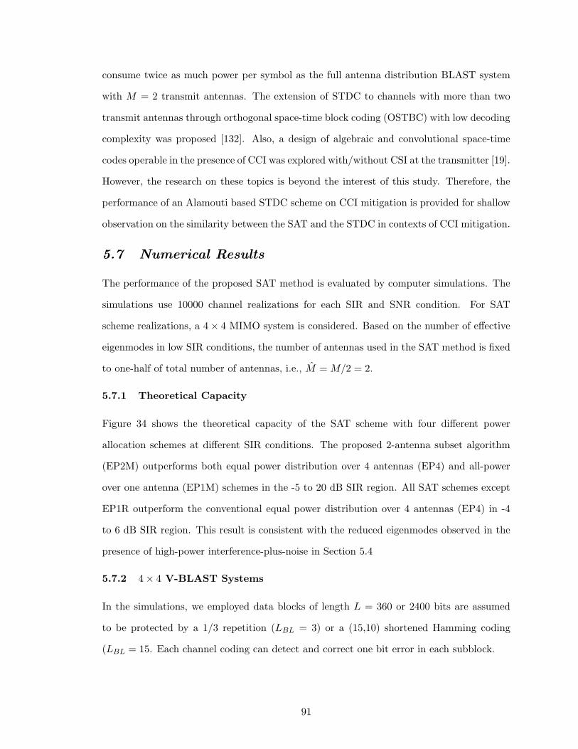
consume twice as much power per symbol as the full antenna distribution BLAST system

with M = 2 transmit antennas. The extension of STDC to channels with more than two

transmit antennas through orthogonal space-time block coding (OSTBC) with low decoding

complexity was proposed [132]. Also, a design of algebraic and convolutional space-time

codes operable in the presence of CCI was explored with/without CSI at the transmitter [19].

However, the research on these topics is beyond the interest of this study. Therefore, the

performance of an Alamouti based STDC scheme on CCI mitigation is provided for shallow

observation on the similarity between the SAT and the STDC in contexts of CCI mitigation.

5.7 Numerical Results

The performance of the proposed SAT method is evaluated by computer simulations. The

simulations use 10000 channel realizations for each SIR and SNR condition. For SAT

scheme realizations, a 4× 4 MIMO system is considered. Based on the number of effective

eigenmodes in low SIR conditions, the number of antennas used in the SAT method is fixed

to one-half of total number of antennas, i.e., M = M/2 = 2.

5.7.1 Theoretical Capacity

Figure 34 shows the theoretical capacity of the SAT scheme with four different power

allocation schemes at different SIR conditions. The proposed 2-antenna subset algorithm

(EP2M) outperforms both equal power distribution over 4 antennas (EP4) and all-power

over one antenna (EP1M) schemes in the -5 to 20 dB SIR region. All SAT schemes except

EP1R outperform the conventional equal power distribution over 4 antennas (EP4) in -4

to 6 dB SIR region. This result is consistent with the reduced eigenmodes observed in the

presence of high-power interference-plus-noise in Section 5.4

5.7.2 4× 4 V-BLAST Systems

In the simulations, we employed data blocks of length L = 360 or 2400 bits are assumed

to be protected by a 1/3 repetition (LBL = 3) or a (15,10) shortened Hamming coding

(LBL = 15. Each channel coding can detect and correct one bit error in each subblock.

91

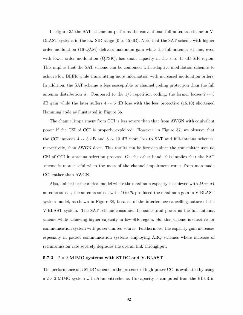
In Figure 35 the SAT scheme outperforms the conventional full antenna scheme in V-

BLAST systems in the low SIR range (0 to 15 dB). Note that the SAT scheme with higher

order modulation (16-QAM) delivers maximum gain while the full-antenna scheme, even

with lower order modulation (QPSK), has small capacity in the 8 to 15 dB SIR region.

This implies that the SAT scheme can be combined with adaptive modulation schemes to

achieve low BLER while transmitting more information with increased modulation orders.

In addition, the SAT scheme is less susceptible to channel coding protection than the full

antenna distribution is. Compared to the 1/3 repetition coding, the former looses 2 ∼ 3

dB gain while the later suffers 4 ∼ 5 dB loss with the less protective (15,10) shortened

Hamming code as illustrated in Figure 36.

The channel impairment from CCI is less severe than that from AWGN with equivalent

power if the CSI of CCI is properly exploited. However, in Figure 37, we observe that

the CCI imposes 4 ∼ 5 dB and 8 ∼ 10 dB more loss to SAT and full-antenna schemes,

respectively, than AWGN does. This results can be foreseen since the transmitter uses no

CSI of CCI in antenna selection process. On the other hand, this implies that the SAT

scheme is more useful when the most of the channel impairment comes from man-made

CCI rather than AWGN.

Also, unlike the theoretical model where the maximum capacity is achieved with MaxM

antenna subset, the antenna subset with Min R produced the maximum gain in V-BLAST

system model, as shown in Figure 38, because of the interference cancelling nature of the

V-BLAST system. The SAT scheme consumes the same total power as the full antenna

scheme while achieving higher capacity in low-SIR region. So, this scheme is effective for

communication system with power-limited source. Furthermore, the capacity gain increases

especially in packet communication systems employing ARQ schemes where increase of

retransmission rate severely degrades the overall link throughput.

5.7.3 2× 2 MIMO systems with STDC and V-BLAST

The performance of a STDC scheme in the presence of high-power CCI is evaluated by using

a 2× 2 MIMO system with Alamouti scheme. Its capacity is computed from the BLER in

92

packet communication links with data blocks size of 360 and 2400 bits. This scheme uses

twice as much power per symbol as the full antenna distribution 2 × 2 BLAST system by

sending a symbol information twice in predefined way. Thus, the STDC scheme traded data

rate for increased transmit power per data symbol. However, as shown in Figure 39 and 40,

the STDC scheme exhibits a similar pattern of capacity gain over 2× 2 V-BLAST scheme

in 5 to 15 dB SIR range by using higher order modulations. Therefore, the STDC scheme

can be considered an alternative adaptive transmission technique in interference dominant

channel conditions. One drawback of the STDC scheme is that it tends to lose capacity

gain as the spatial code rate rs decreases.

93

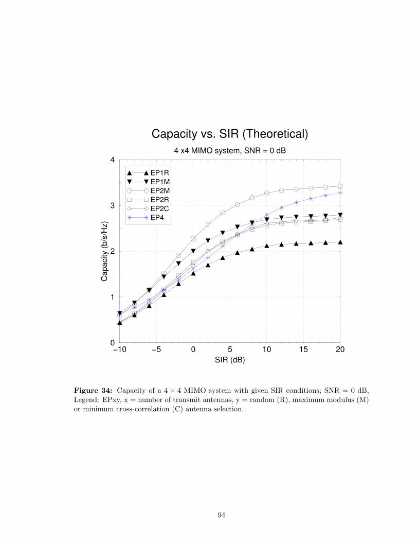
−10 −5 0 5 10 15 20SIR (dB)

0

1

2

3

4

Cap

acity

(b/s

/Hz)

Capacity vs. SIR (Theoretical)4 x4 MIMO system, SNR = 0 dB

EP1REP1MEP2MEP2REP2CEP4

Figure 34: Capacity of a 4 × 4 MIMO system with given SIR conditions; SNR = 0 dB,Legend: EPxy, x = number of transmit antennas, y = random (R), maximum modulus (M)or minimum cross-correlation (C) antenna selection.

94

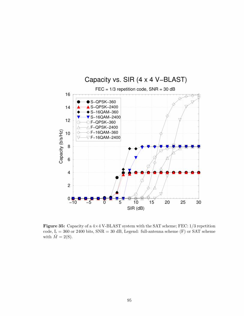
−10 −5 0 5 10 15 20 25 30SIR (dB)

0

2

4

6

8

10

12

14

16

Cap

acity

(b/s

/Hz)

Capacity vs. SIR (4 x 4 V−BLAST)FEC = 1/3 repetition code, SNR = 30 dB

S−QPSK−360S−QPSK−2400S−16QAM−360S−16QAM−2400F−QPSK−360F−QPSK−2400F−16QAM−360F−16QAM−2400

Figure 35: Capacity of a 4×4 V-BLAST system with the SAT scheme; FEC: 1/3 repetitioncode, L = 360 or 2400 bits, SNR = 30 dB, Legend: full-antenna scheme (F) or SAT schemewith M = 2(S).

95

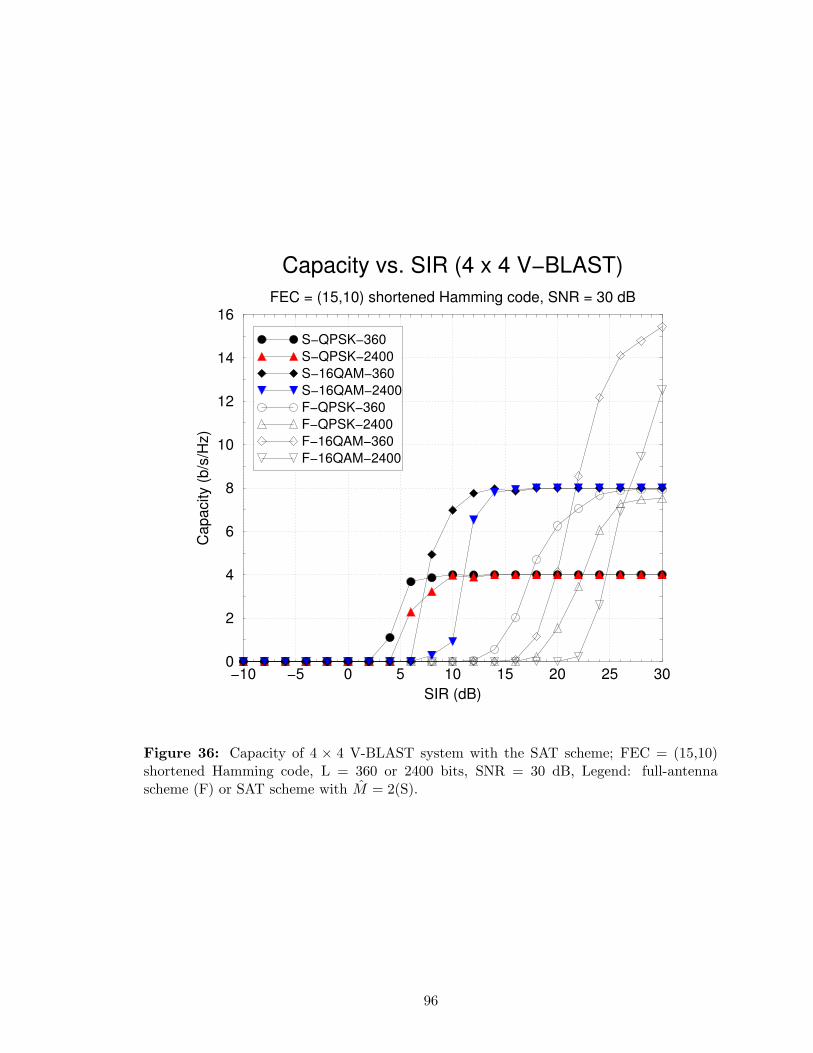
−10 −5 0 5 10 15 20 25 30SIR (dB)

0

2

4

6

8

10

12

14

16

Cap

acity

(b/s

/Hz)

Capacity vs. SIR (4 x 4 V−BLAST)FEC = (15,10) shortened Hamming code, SNR = 30 dB

S−QPSK−360S−QPSK−2400S−16QAM−360S−16QAM−2400F−QPSK−360F−QPSK−2400F−16QAM−360F−16QAM−2400

Figure 36: Capacity of 4 × 4 V-BLAST system with the SAT scheme; FEC = (15,10)shortened Hamming code, L = 360 or 2400 bits, SNR = 30 dB, Legend: full-antennascheme (F) or SAT scheme with M = 2(S).

96

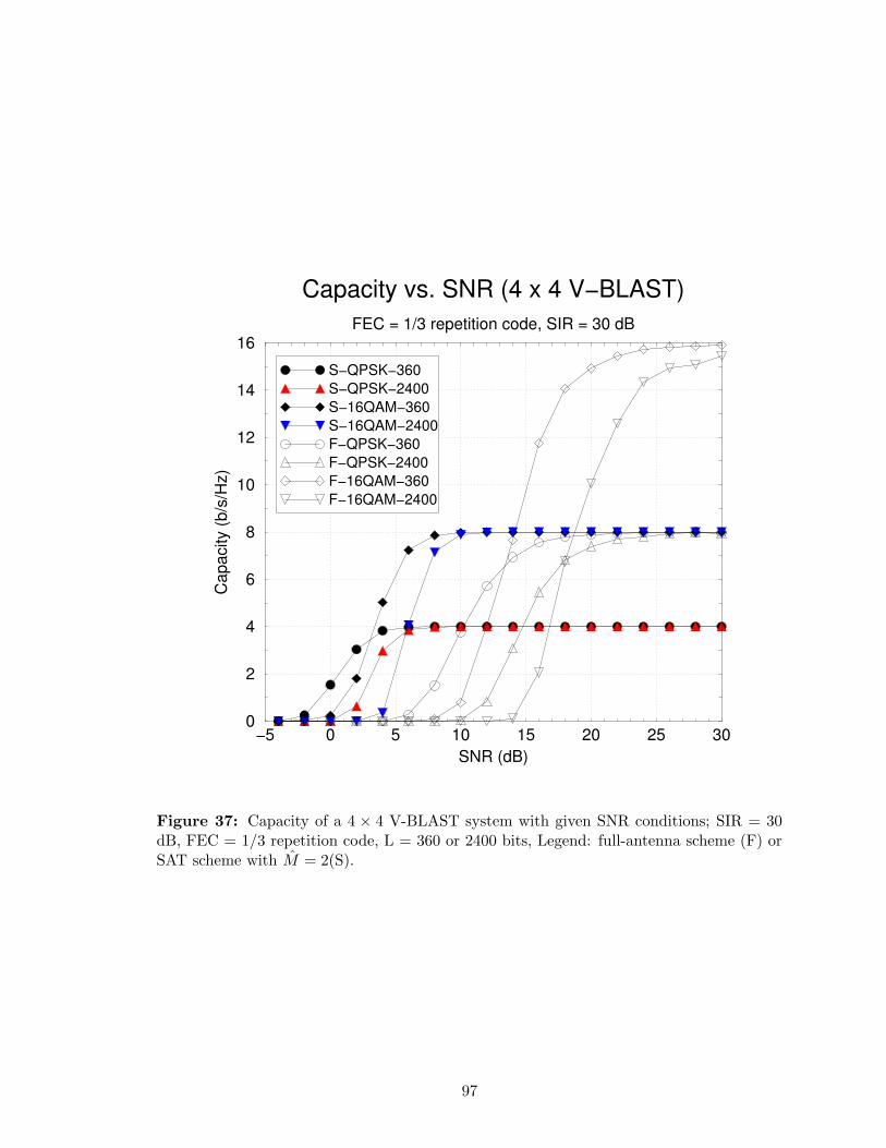
−5 0 5 10 15 20 25 30SNR (dB)

0

2

4

6

8

10

12

14

16

Cap

acity

(b/s

/Hz)

Capacity vs. SNR (4 x 4 V−BLAST)FEC = 1/3 repetition code, SIR = 30 dB

S−QPSK−360S−QPSK−2400S−16QAM−360S−16QAM−2400F−QPSK−360F−QPSK−2400F−16QAM−360F−16QAM−2400

Figure 37: Capacity of a 4 × 4 V-BLAST system with given SNR conditions; SIR = 30dB, FEC = 1/3 repetition code, L = 360 or 2400 bits, Legend: full-antenna scheme (F) orSAT scheme with M = 2(S).

97

−10 −5 0 5 10 15 20 25 30SIR (dB)

10−4

10−3

10−2

10−1

100

BE

R

Antenna Selection Metric4 x 4 V−BLAST MIMO system

QPSK−MMQPSK−RAQPSK−MCQPSK−Full16QAM−MM16QAM−RA16QAM−MC16QAM−Full

Figure 38: BER performance of antenna subset selection criteria for a 4 × 4 V-BLASTsystem with M = 2; SNR = 30dB, Legend: maximum modulus (MM), random (RA) orminimum cross-correlation (MC) antenna selection.

98

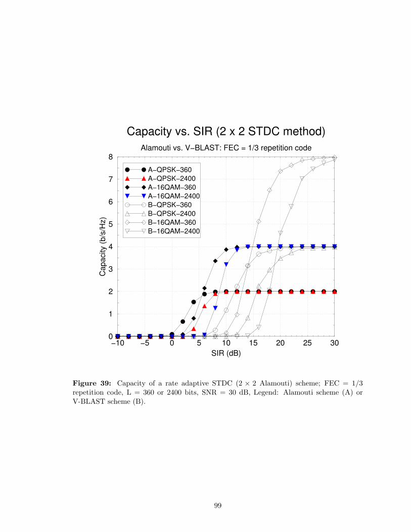
−10 −5 0 5 10 15 20 25 30SIR (dB)

0

1

2

3

4

5

6

7

8

Cap

acity

(b/s

/Hz)

Capacity vs. SIR (2 x 2 STDC method)Alamouti vs. V−BLAST: FEC = 1/3 repetition code

A−QPSK−360A−QPSK−2400A−16QAM−360A−16QAM−2400B−QPSK−360B−QPSK−2400B−16QAM−360B−16QAM−2400

Figure 39: Capacity of a rate adaptive STDC (2 × 2 Alamouti) scheme; FEC = 1/3repetition code, L = 360 or 2400 bits, SNR = 30 dB, Legend: Alamouti scheme (A) orV-BLAST scheme (B).

99

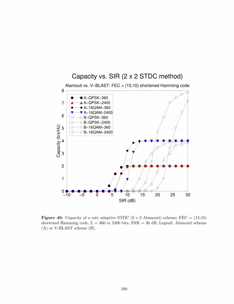
−10 −5 0 5 10 15 20 25 30SIR (dB)

0

1

2

3

4

5

6

7

8

Cap

acity

(b/s

/Hz)

Capacity vs. SIR (2 x 2 STDC method)Alamouti vs. V−BLAST: FEC = (15,10) shortened Hamming code

A−QPSK−360A−QPSK−2400A−16QAM−360A−16QAM−2400B−QPSK−360B−QPSK−2400B−16QAM−360B−16QAM−2400

Figure 40: Capacity of a rate adaptive STDC (2 × 2 Alamouti) scheme; FEC = (15,10)shortened Hamming code, L = 360 or 2400 bits, SNR = 30 dB, Legend: Alamouti scheme(A) or V-BLAST scheme (B).

100

CHAPTER VI

CONCLUDING REMARKS

This dissertation has considered several topics in interference mitigation for practical wire-

less communication systems in contexts of receiver design, channel estimation, link-level

performance evaluation, and capacity analysis. The research work is primarily focused to

address the problems in the design of interference resilient receivers or transmitters in the

following areas:

• joint-detection IC-DDF ML Bluetooth receiver

• joint-detection interference rejection combining TDMA receiver

• interference resilient power allocation in MIMO systems

6.1 Summary of Contributions

In Chapter 3, we proposed an interference cancelling dual decision feedback (IC-DDF)

receiver that jointly detects two colliding Bluetooth signals to mitigate the packet error

probability in the low-Doppler flat fading channels. For a particular case of systems with

a single antenna for economic solutions, the dual decision feedback scheme minimizes the

CCI and the self interference from the shaping pulse simultaneously. An RLS-type channel

estimator, based on the random walk model and constant covariance matrix, is employed to

perform joint channel estimation and tracking function with reduced complexity. The pro-

posed receiver achieved large gains in -12 to 4 dB CIR range over a conventional frequency

discriminator type receiver, and showed its resilience to channel variations, especially in

typical Bluetooth operating environments. In addition, a system level performance evalua-

tion is addressed for an interference resilient receiver in frequent packet collisions by using

a geometric approach. In the proposed scheme, the pdf of the received CIR is derived from

the traffic load distributions and the network topology of collocated Bluetooth piconets.

101

For overall link throughput assessment, we also derived a generalized packet collision prob-

abilities for the multiple collocated Bluetooth piconets carrying combined traffics of ACL

and SCO links.

In Chapter 4, we proposed a soft output fractionally spaced IRC-DDFSE receiver that

jointly detects two co-channel binary (GSM) and non-binary (EDGE) TDMA signals in

frequency selective channels for an extended range signal reception. The proposed receiver

decodes signals from remote base stations in the presence of strong CCI from a nearby

co-channel base station at received CIR less than -10 dB. The joint-detection IRC structure

mitigates the influence from a strong CCI. The increased complexity of the joint detection

architecture is diminished by using a DDFSE technique. Concatenated Viterbi and Log-

MAP algorithms improved the probability of correct sequence estimation by generating soft

outputs for the outer code decodings of binary (GMSK) and non-binary (8PSK) symbols.

For the completeness of the Log-MAP function, Viterbi algorithm generates a unique covari-

ance matrix and a corresponding decision feedback sequence for each state of the Log-MAP

function by using a PSP algorithm. Joint channel estimation with an LS criterion reduces

the channel estimation error from the cross-correlation between the TSSs of two co-channel

signals. The fractionally-spaced receiver structure whitens the colored noise and reduces

the performance degradation from the delay offset between the two co-channel signals. We

also showed that an NBAA preprocessing combined with an interference cancelling receiver

is effective for the extended range signal reception in TDMA cellular systems. In addition,

the proposed receiver showed its resilience to the imbalanced CCI across antenna branches

in low-CIR conditions.

In Chapter 5, we proposed an adaptive power allocation scheme for MIMO systems by

using subset antenna transmission (SAT) techniques to increase the spectral efficiency in the

presence of co-channel interference (CCI). This scheme uses the phenomena of unbalanced

eigenmodes in channel matrices often observed in the presence of high-power interference

or noise. The phenomena, which can be explained by large condition numbers in channel

matrices, results in a capacity loss in the equal power distribution scheme. In the proposed

scheme, the capacity loss is reduced by allocating transmit power equally on a selected

102

subset of the transmit antennas. From the results of numerical analysis, we observed that

the proposed scheme achieves larger capacity than that of the all-antenna transmission

method when the received SIR is very low, or the channel matrix is ill conditioned. The

proposed scheme outperformed the conventional method in low SIR or SNR conditions not

only in information theoretic capacity but also in the capacity of V-BLAST MIMO sys-

tems. Furthermore, the proposed scheme combined with an adaptive modulation technique

outperforms the all-antenna transmission scheme by achieving low BLER even in higher

modulation order. For the selection of an antenna subset for transmission in V-BLAST sys-

tems, a set of antenna having minimum crosscorrelation produces maximum capacity gain

by exploiting the successive interference cancellation nature of the V-BLAST architecture.

6.2 Suggestions for Further Research

Future research can proceed along several lines.

Interference Mitigating Receiver Design:

• In ISM bands, many systems with different radio interface coexist and interfere to each

other. Although the issues of coexistence and interference mitigation has received

much attention in literature, comparatively little can be found describing practical

solutions for inter-system interference. Both PHY and MAC layer approaches can be

used in separate or integrative methods.

• In most literature on joint detection or interference mitigation receiver designs, the

receiver assumes a priori knowledge on the existence of interference. However, when

the interference is arriving in asynchronous and variable length burst formats, the

detection of interfering signals is an essential function to achieve the desired perfor-

mance. It becomes a challenging task in frequency bands where the radio spectrum is

shared by communication systems with heterogeneous radio interfaces. Furthermore,

interference detection can be an important step to the design of a receiver for multi-

format signal reception and transmission. A software defined radio (SDR) architecture

is an example of possible applications.

103

Transmitter Design for Interference Resilient MIMO Systems:

• An extended proof of the conjecture that the SAT model achieves capacity gain in

low transmit power or small eigenmodes cases needs further research. It includes the

study on the distribution of the eigenvalues of the Wishart matrix.

• The SAT scheme is focused on power control over selected antenna subset. It can

be extended by using precoding and rate adaptation. Alamouti type STBC is a

primitive example of precoding for interference mitigation. Also, the SAT scheme can

be extended to multiple antenna-set partitioning combined with rate adaptive STBC

techniques in context of overall capacity maximization.

• Interlayer design approaches have received much attention for optimum link through-

put in time-varying channel and interference conditions. Its adaptive feature can be

extended to interference mitigation by employing subset antenna transmission, adap-

tive modulation, and interference identification techniques. The open- and closed-loop

control for adaptive transmission can be another research concern in interference can-

celling interlayer designs. Interference-adaptive interlayer design combined with an

SDR architecture can be one realization of the cognitive radio (CR) initiative.

104

REFERENCES

[1] IEEE, “Wireless LAN Medium Access Control (MAC) and Physical Layer (PHY)Specification,” 802.11, 1997.

[2] ETSI, “Digital Cellular Telecommunications System (Phase 2+): Channel Coding,”GSM-05.03, 1999.

[3] ETSI, “Digital Cellular Telecommunications System (Phase 2+): Modulation,” GSM-05.04, 1999.

[4] ETSI, “Digital Cellular Telecommunications System (Phase 2+): Multiplexing andMultiple Access on the Radio Path,” GSM-05.02, 1999.

[5] TIA, “Mobile Station-Base Station Compatibility Standard for Wideband SpreadSpectrum Cellular Systems,” TIA/EIA-95-B, 1999.

[6] Bluetooth SIG, “Specification of the Bluetooth System,” Version 1.0, 1999.

[7] TIA, “Physical Layer Specification for CDMA Spread Spectrum CommunicationsSystem,” TIA/EIA IS-2000, 2000.

[8] 3GPP, “3GPP TSG RAN WG4; Physical Layer Procedures (FDD),” 3GPP TS 25.214,2000-03.

[9] IEEE, “Air Interface for Fixed Broadband Wireless Access Systems - Medium AccessControl and Additional Physical Layer Specifications for 2-11 GHz,” 802.16a, 2003.

[10] IEEE, “Low-Rate Wireless PAN Medium Access Control (MAC) and Physical Layer(PHY) Specification,” 802.15.4, 2003.

[11] 3GPP, “3GPP TSG GERAN; Radio Transmission and Reception,” 3GPP TS 45.005,Release 5.

[12] Aalo, V. A. and Zhang, J., “Performance of Antenna Array Systems with OptimumCombining in a Rayleigh Fading Environment,” IEEE Commun. Lett., vol. 4, pp. 387–389, Dec. 2000.

[13] Agrawal, A., Andrews, J. G., Cioffi, J. M., and Meng, T., “Iterative PowerControl for Imperfect Successive Interference Cancellation,” IEEE Trans. WirelessCommun., vol. 4, pp. 878–884, May 2005.

[14] Alamouti, S., “A Simple Transmit Diversity Technique for Wireless Communica-tions,” IEEE J. Select. Areas Commun., pp. 1451–1458, Oct. 1998.

[15] Anderson, S., Hagerman, B., Dam, H., Forssen, U., Karlsson, J., Kronest-

edt, F., and Mazur, S., “Adaptive Antennas for GSM and TDMA Systems,” IEEEPersonal Commun. Mag., vol. 6, pp. 74–86, June 1999.

105

[16] Andrews, J. G., “Interference Cancellation for Cellular Systems: A ContemporaryOverview,” IEEE Wireless Commun. Mag., vol. 12, pp. 19–29, Apr. 2005.

[17] Andrews, J. G. and Meng, T. H., “Optimum Power Control for Successive In-terference Cancellation with Imperfect Channel Estimation,” IEEE Trans. WirelessCommun., vol. 2, pp. 375–383, Mar. 2003.

[18] Ariyavisitakul, S. L., Winters, J. H., and Sollenberger, N. R., “Joint Equal-ization and Interference Suppression for High Data Rate Wireless Systems,” IEEE J.Select. Areas Commun., vol. 18, pp. 1214–1220, July 2000.

[19] Arunachalam, A. and Gamal, H. E., “Space-Time Coding for MIMO Systemswith Co-Channel Interference,” IEEE Trans. Wireless Commun., vol. 3, pp. 1953–1958, Nov. 2004.

[20] Austin, M., “SAIC and Synchronized Networks for Increased GSM Capacity,” WhitePaper, 3G Americas’ SAIC working group, Sept. 2003.

[21] Bahl, L. R., Cocke, J., Jelinek, F., and Raviv, J., “Optimal Decoding of LinearCodes for Minimizing Symbol Error Rate,” IEEE Trans. Inform. Theory, vol. 20,pp. 284–287, Mar. 1974.

[22] Banister, B. C. and Zeidler, J. R., “Transmission Subspace Tracking forMIMO Communications Systems,” in Proc. IEEE Global Communications Confer-ence, GLOBECOM ’01, pp. 1680–1686, Nov. 2001.

[23] Benjebbour, A. and Yoshida, S., “On the Relation between Ordering Metrics forZF and MMSE Successive Detection in MIMO Systems,” IEICE Transactions onCommunications, vol. E87-B, pp. 2021–2027, June 2004.

[24] Berenguer, I., Wang, X., and Wassell, I. J., “Transmit Antenna Selection inLinear Receivers: Geometrical Approach,” Electronics Letters, vol. 40, pp. 292–293,Mar. 2004.

[25] Bischl, H. and Lutz, E., “Packet Error Rate in the Non-Interleaved Rayleigh Chan-nel,” IEEE Trans. Commun., vol. 43, pp. 1375–1382, Feb. 1995.

[26] Blum, R., “MIMO Capacity with Interference,” IEEE J. Select. Areas Commun.,vol. 21, pp. 793–801, June 2003.

[27] Bottomley, G. E. and Jamal, K., “Adaptive Arrays and MLSE Equalization,” inProc. IEEE Vehicular Technology Conference, VTC ’95, pp. 50–54, July 1995.

[28] Bottomley, G. E., Molnar, K. J., and Chennakeshu, S., “Interference Cancel-lation with an Array Processing MLSE Receiver,” IEEE Trans. Veh. Technol., vol. 48,pp. 1321–1331, Sept. 1999.

[29] Buehrer, R. M., Kaul, A., Striglis, S., and Woerner, B. D., “Analysis ofDS-CDMA Parallel Interference Cancellation with Phase and Timing Errors,” IEEEJ. Select. Areas Commun., vol. 14, pp. 1522–1535, Oct. 1996.

[30] Catreux, S., Driessen, P. F., and Greenstein, L. J., “Attainable Throughput ofan Interference-Limited Multiple-Input Multiple-Output (MIMO) Cellular System,”IEEE Trans. Commun., vol. 49, pp. 1307–1311, Aug. 2001.

106

[31] Chuang, J., Cimini, L. J., Li, G. Y., Mcnair, B., Sollenberger, N., Zhao, H.,Lin, L., and Suzuki, M., “High-Speed Wireless Data Access Based on CombiningEDGE with Wideband OFDM,” IEEE Commun. Mag., pp. 92–98, Nov. 1999.

[32] Cingular, “SAIC System Level Evaluations Based on GERAN System Simulator.”3GPP TSG-GERAN 15 Tdoc GP-031270, 2003.

[33] Cordeiro, C. M. and Agrawal, D. P., “Piconet Interference Modeling and Per-formance Evaluation of Bluetooth MAC Protocol,” in Proc. IEEE Global Communi-cations Conference, GLOBECOM ’01, pp. 25–29, Nov. 2001.

[34] Cover, T. M. and Thomas, J. A., Elements of Information Theory. New York:John Wiley and Sons, 1991.

[35] Debbah, M., Muquet, B., Courville, M., Muck, M., Simoens, S., and Louba-

ton, P., “A MMSE Successive Interference Cancellation Scheme for a New AdjustableHybrid Spread OFDM Systems,” in Proc. IEEE Vehicular Technology Conference,VTC ’00, pp. 745–749, May 2000.

[36] Demirkol, M. F. and Ingram, M. A., “Power-Controlled Capacity for InterferingMIMO Links,” in Proc. IEEE Vehicular Technology Conference, VTC ’01, pp. 187–191, Oct. 2001.

[37] Derryberry, R. T., Gray, S. D., Ionescu, D. M., Mandyam, G., andRaghothaman, B., “Transmit Diversity in 3G CDMA Systems,” IEEE Commun.Mag., vol. 40, pp. 68–75, Apr. 2002.

[38] Duel-Hallen, A., “Equalizers for Multiple Input/Multiple Output Channels andPAM Systems with Cyclostationary Input Sequences,” IEEE J. Select. Areas Com-mun., vol. 10, pp. 630–639, Apr. 1992.

[39] Duel-Hallen, A., “Decorrelating Decision Feedback Multiuser Detector for Syn-chronous Code-Division Multiple Access Channel,” IEEE Trans. Commun., vol. 41,pp. 285–290, Feb. 1993.

[40] Duel-Hallen, A., “A Family of Multiuser Decision-Feedback Detectors for Asyn-chronous Code-Division Multiple Access Channels,” IEEE Trans. Commun., vol. 43,pp. 421–434, Feb. 1995.

[41] Duel-Hallen, A. and Heegard, C., “Delayed Decision Feedback Sequence Esti-mation,” IEEE Trans. Commun., vol. 37, pp. 428–436, May 1989.

[42] Edelman, A., Eigenvalues and Condition Numbers of Random Matrices. PhD thesis,Massachusetts Institute of Technology, Cambridge, May 1989.

[43] El-Hoiydi, A., “Interference Between Bluetooth Networks-Upper Bound on thePacket Error Rate,” IEEE Commun. Lett., vol. 5, pp. 245–247, June 2001.

[44] Eleftheriou, E. and Falconern, D. D., “Tracking Properties and Steady-StatePerformance of RLS Adaptive Filter Algorithms,” IEEE Trans. Acoust., Speech, Sig-nal Processing, vol. 34, pp. 1097–1110, Oct. 1986.

107

[45] Ennis, G., “Impact of Bluetooth on 802.11 Direct Sequence Wireless LANs.” IEEE802.11 Contribution 98/319a, 1998.

[46] Etten, W. V., “Maximum Likelihood Receiver for Multiple Channel TransmissionSystems,” IEEE Trans. Commun., vol. 24, pp. 276–283, Feb. 1976.

[47] Eyuboglu, M. V. and Qureshi, S. U., “Reduced-State Sequence Estimation forCoded Modulation on Intersymbol Interference Channels,” IEEE J. Select. AreasCommun., vol. 7, pp. 989–995, Aug. 1989.

[48] Farrokhi, F. R., Foschini, G. J., Lozano, A., and Valenzuela, R. A., “Link-Optimal Space-Time Processing with Multiple Transmit and Receive Antennas,”IEEE Commun. Lett., vol. 5, pp. 85–87, Mar. 2001.

[49] Ferguson, P. and Huston, G., Quality of Service: Delivering QoS on the Internetand in Corporate Networks. New York: John Wiley and Sons, 1998.

[50] Forney, Jr., G. D., “Maximum Likelihood Sequence Estimation of Digital Se-quences in the Presence of Intersymbol Interference,” IEEE Trans. Inform. Theory,vol. 18, pp. 363–378, May 1972.

[51] Foschini, G. J., “Layered Space-Time Architecture for Wireless Communicationin a Fading Environment When Using Multiple Antennas,” Bell Systems TechnicalJournal, vol. 1, pp. 41–59, 1996.

[52] Foschini, G. J. and Gans, M. J., “On the Limits of Wireless Communications ina Fading Environment when using Multiple Antennas,” Kluwer Journal of WirelessPersonal Communications, vol. 6, pp. 315–335, 1998.

[53] Friedlander, B. and Scherzer, S., “Beamforming vs. Transmit Diversity in theDownlink of a Cellular Communications System,” in Proc. IEEE Thirty-Fifth Asilo-mar Conference, pp. 1014–1018, Nov. 2001.

[54] Fukawa, K. and Suzuki, H., “Blind Interference Cancelling Equalizer for Mobile Ra-dio Communications,” IEICE Transactions on Communications, vol. E77-B, pp. 580–588, 1994.

[55] Garg, V. K. and Wilkes, J. E., Wireless and Personal Communications Systems.Upper Saddle River, NJ: Prentice Hall, 1995.

[56] Gaston, D., “Overcoming Interference in the Spread Spectrum ISM Bands,” in Proc.of WESCON ’95, pp. 491–496, May 1995.

[57] Gaur, S. and Ingram, M. A., “Transmit/Receive Antenna Selection for MIMOSystems to Improve Error Performance of Linear Receivers,” in Proc. ITC/IEEEWorkshop on Smart Antennas, WSA 2005, Apr. 2005.

[58] Gaur, S., Jiang, J. S., Ingram, M. A., and Demirkol, M. F., “Interfering MIMOLinks with Stream Control and Optimal Antenna Selection,” in Proc. IEEE GlobalCommunications Conference, GLOBECOM ’04, pp. 3138–3142, Nov. 2004.

[59] Gerstacker, W. H. and Schober, R., “Equalization Concepts for EDGE,” IEEETrans. Wireless Commun., vol. 1, pp. 190–199, 2002.

108

[60] Gesbert, D., Shafi, M., Shiu, D. S., Smith, P. J., and Naguib, A., “FromTheory to Practice: An Overview of MIMO Space-Time Coded Wireless Systems,”IEEE J. Select. Areas Commun., vol. 21, pp. 281–302, 2003.

[61] Getu, B. N., Andersen, J. B., and Faserotu, J. R., “MIMO Systems: Optimiz-ing the Use of Eigenmodes,” in Proc. IEEE Intl. Symposium on Personal, Indoor andMobile Radio Communications, PIMRC ’03, pp. 1129–1133, Sept. 2003.

[62] Gibson, J. D., Mobile Communications Handbook, 2nd ed. Secaucus: Springer-VerlagNew York, 1999.

[63] Godara, L. C., “Applications of Antenna Arrays to Mobile Communications. I.Performance Improvement, Feasibility, and System Considerations,” in Proceedingsof the IEEE, vol. 85, pp. 1031–1060, July 1997.

[64] Goldsmith, A. J., Jafar, S. A., Jindal, N., , and Vishwanath, S., “CapacityLimits of MIMO Channels,” IEEE J. Select. Areas Commun., vol. 21, pp. 684–702,June 2003.

[65] Golmie, N., Chevrollier, N., and ElBakkouri, I., “Interference Aware Blue-tooth Packet Scheduling,” in Proc. IEEE Global Communications Conference,GLOBECOM ’01, pp. 2857–2863, Nov. 2001.

[66] Golmie, N. and Mouveaux, F., “Impact of Interference on the Bluetooth Ac-cess Control Performance: Preliminary Results.” IEEE 802.15 Contribution 00/322r0,2000.

[67] Goodman, D. J. and Saleh, A. A. M., “The Near-Far Effect in Local Aloha RadioCommunications,” IEEE Trans. Veh. Technol., vol. 36, pp. 19–27, Feb. 1987.

[68] Gore, D. A., Gorokhov, A., and Paulraj, A., “Joint MMSE Versus V-BLASTand Antenna Selection,” in Proceedings of The Thirty-Sixth Asilomar Conference,vol. 1, pp. 505–509, Nov. 2002.

[69] Gore, D. A., R. W. Heath, J., and Paulraj, A., “Transmit Selection in SpatialMultiplexing Systems,” IEEE Commun. Lett., vol. 6, pp. 91–493, Nov. 2002.

[70] Gorokhov, A., Collados, M., Gore, D., and Paulraj, A., “Transmit/ReceiveMIMO Antenna Subset Selection,” in Proc. IEEE Intl. Conference on Acoustics,Speech, and Signal Processing, ICASSP ’04, pp. 13–16, May 2004.

[71] Hafeez, A., Hui, D., and Arslan, H., “Interference Cancellation for EDGE viaTwo-User Joint Demodulation,” in Proc. IEEE Vehicular Technology Conference,VTC ’03, pp. 1025–1029, Oct. 2003.

[72] Hafeez, A., Molnar, K. J., Bottomley, G. E., and Ramesh, R., “Capacity andQuality Enhancement for ANSI-136 Downlink Using Interference Cancellation andBeamforming,” in Proc. IEEE Vehicular Technology Conference, VTC ’00, pp. 2414–2421, Sept. 2000.

[73] Hamied, K. and Stuber, G. L., “A Fractionally-Spaced MLSE Receiver,” in Proc.IEEE Conference on Communication, ICC ’95, pp. 7–11, May 1995.

109

[74] Haustein, T. and Boche, H., “Optimal Power Allocation for MSE and Bit-Loadingin MIMO Systems and the Impact of Correlation,” in Proc. IEEE Intl. Conferenceon Acoustics, Speech, and Signal Processing, ICASSP ’03, pp. 405–408, Apr. 2003.

[75] Haykin, S., Adaptive Filter Theory. Englewood Cliffs: Prentice-Hall, 1991.

[76] Hoeher, P. A., Badri-Hoeher, S., Deng, S., Krakowski, C., and Xu, W.,“Joint Delayed-Decision Feedback Sequence Estimation with Adaptive State Allo-cation,” in Proc. International Symposium on Information Technology, ISIT 2004,p. 132, July 2004.

[77] Hoeher, P. A., Badri-Hoeher, S., Xu, W., and Krakowski, C., “Single-Antenna Co-Channel Interference Cancellation for TDMA Cellular Radio Rystems,”IEEE Wireless Commun. Mag., vol. 12, pp. 30–37, Apr. 2005.

[78] Horn, R. A. and Johnson, C. R., Matrix Computations. Cambridge, U.K.: Cam-bridge University Press, 1985.

[79] Howitt, I., “WLAN and WPAN Coexistence in UL Band,” IEEE Trans. Veh. Tech-nol., vol. 50, pp. 1114–1124, July 2001.

[80] Howitt, I., “Mutual Interference Between Independent Bluetooth Piconets,” IEEETrans. Veh. Technol., vol. 52, pp. 708–718, May 2003.

[81] Howitt, I. and Hawwar, V. K., “Evaluation of Outage Probability Due to Cochan-nel Interference in Fading for a TDMA System with a Beamformer,” in Proc. IEEEVehicular Technology Conference, VTC ’98, pp. 520–524, May 1998.

[82] Jakes, W. C., Microwave Mobile Communications. New York: IEEE Press, 1994.

[83] Janssen, G. J. M., Stigter, P. A., and Prasad, R., “Wideband Indoor ChannelMeasurements and BER Analysis of Frequency Selective Multipath Channels at 2.4,4.75, and 11.5 Ghz,” IEEE Trans. Commun., vol. 44, pp. 1272–1288, Oct. 1996.

[84] Joung, J. and Stuber, G. L., “Fractionally Spaced IRC-DDFSE for TDMA CellularSystems,” in Proc. IEEE Vehicular Technology Conference, VTC ’99, pp. 441–445,Sept. 1999.

[85] Kamerman, A., “Coexistence between Bluetooth and IEEE 802.11 CCK Solutionsto Avoid Mutual Interference.” IEEE 802.11 Contribution 00/162, 2000.

[86] Karlsson, J. and Heinegøard, J., “Interference Rejection Combining for GSM,”in Proc. IEEE Intl. Conference on Universal Personal Communications, ICUPC ’96,pp. 433–437, Sept. 1996.

[87] Kim, K. and Stuber, G. L., “Interference Mitigation in Asynchronous Slow Fre-quency Hopping Bluetooth Networks,” Kluwer Journal of Wireless Personal Com-munications, vol. 28, pp. 143–159, Jan. 2004.

[88] Kim, K. and Stuber, G. L., “Range Extended Interference Cancelling Joint De-tection TDMA Receiver,” in Proc. International Symposium on Wireless PersonalMultimedia Communications, WPMC ’04, pp. 315–319, Sept. 2004.

110

[89] Kim, K. and Stuber, G. L., “Joint Detection Interference Rejection CombiningGSM/EDGE Receiver,” Submitted to IEEE Trans. on Wireless Communications Let-ter, Jan. 2005.

[90] Kim, S. C., Bertoni, H. L., and Stern, M., “Pulse Propagation Characteristicsat 2.4 GHz Inside Buildings,” IEEE Trans. Veh. Technol., vol. 45, pp. 579–592, Aug.1996.

[91] Kohno, R., Meiden, R., and Milstein, L. B., “Spread-Spectrum Access Methodfor Wireless Communications,” IEEE Commun. Mag., vol. 33, pp. 58–67, Jan. 1995.

[92] Lai, J. and Mandayam, N., “Packet Error Rate for Burst-error-correcting Codes inRayleigh Fading Channels,” in Proc. IEEE Vehicular Technology Conference, VTC’98, pp. 1568–1572, May 1998.

[93] Laster, J. D. and Reed, J. H., “Interference Rejection in Digital Wireless Com-munications,” IEEE Signal Processing Mag., vol. 14, pp. 37–62, May 1997.

[94] Lee, W. C. Y., Mobile Communication Engineering. New York: McGraw-Hill, 1982.

[95] Li, L., Li, H., and Yao, Y. D., “Intersymbol/Cochannel Interference Cancellationfor Transmit Diversity Systems in Frequency Selective Fading Channels,” in Proc.IEEE Vehicular Technology Conference, VTC ’01, pp. 678–682, Oct. 2001.

[96] Li, Y., Winters, J. H., and Sollenberger, N., “Spatial-Temporal Equalizationfor IS-136 Systems with Rapid Dispersive Fading and Co-Channel Interference,” IEEETrans. Veh. Technol., vol. 48, pp. 1182–1194, July 1999.

[97] Liang, J., Paulraj, A. J., and Singh, A., “Two Stage CCI/ISI Reduction withSpace-Time Processing in TDMA Cellular Networks,” in Proc. IEEE Thirty AsilomarConference, pp. 607–611, Nov. 1996.

[98] Lin, J., Ling, F., and Proakis, J. G., “Fading Channel Tracking Properties ofSeveral Adaptive Algorithms for the North American Digital Cellular System,” inProc. IEEE Vehicular Technology Conference, VTC ’91, pp. 273–276, May 1993.

[99] Lin, S. C. and Prabhu, V. K., “Diversity Combining and Equalization ofFrequency-Selective Fading Signals with Unequal Mean Strengths,” in Proc. IEEEVehicular Technology Conference, VTC ’98, pp. 753–757, May 1998.

[100] Lo, N. W. K., Falconer, D., and Sheikh, A. U. H., “Adaptive Equalization forCo-Channel Interference in a Multipath Fading Environment,” IEEE Trans. Com-mun., vol. 43, pp. 1441–1453, Feb. 1995.

[101] Lupas, R. and Verdu, S., “Linear Multiuser Detectors for Synchronous Code-Division Multiple-Access Channels,” IEEE Trans. Veh. Technol., vol. 35, pp. 123–136,Apr. 1989.

[102] Lupas, R. and Verdu, S., “Near-Far Resistance of Multiuser Detectors in Asyn-chronous Channels,” IEEE Trans. Commun., vol. 38, pp. 496–508, Apr. 1990.

[103] Mallik, R. K., Win, M. Z., and Winters, J. H., “Performance of Dual-DiversityPredetection EGC in Correlated Rayleigh Fading with Unequal Branch SNRs,” IEEETrans. Commun., vol. 50, pp. 1041–1044, July 2002.

111

[104] Margarita, A., Flores, S. J., Rubio, L., Almenar, V., and Corral, J. L.,“Application of MUSIC for Spatial Reference Beamforming for SDMA in a SmartAntenna for GSM and DECT,” in Proc. IEEE Vehicular Technology Conference,VTC ’01, pp. 123–126, May 2001.

[105] Oja, E., Subspace Methods of Pattern Recognition. Hertfordshire: Research StudiesPress, 1983.

[106] Palomar, D. P., Cioffi, J. M., and Lagunas, M. A., “Uniform Power Allocationin MIMO Channels: a Game-Theoretic Approach,” IEEE Trans. Inform. Theory,vol. 49, pp. 1707–1727, July 2003.

[107] Park, M., Heath, R. M., and Nettles, S. M., “Improving Throughput and Fair-ness for MIMO Ad-Hoc Networks Using Antenna Selection Diversity,” in Proc. IEEEGlobal Communications Conference, GLOBECOM ’04, pp. 3363–3367, Nov. 2004.

[108] Parsons, J. D., The Mobile Radio Propagation Channel. London, U.K.: PentechPress, 1992.

[109] Patel, P. and Holtzman, J., “Analysis of a Simple Successive Interference Can-cellation Scheme in a DS/CDMA System,” IEEE J. Select. Areas Commun., vol. 12,pp. 796–807, June 1994.

[110] Paulraj, A. J., Gore, D. A., Nabar, R. U., and Bolcskei, H., “An Overviewof MIMO Communications-A Key to Gigabit Wireless,” in Proceedings of The IEEE,vol. 92, pp. 198–218, Feb. 2004.

[111] Payaro, M., Mestre, X., and Lagunas, M. A., “Optimum Transmit Architectureof a MIMO System Under Modulus Channel Knowledge at the Transmitter,” in Proc.IEEE Information Theory Workshop, ITW ’04, pp. 174–178, Oct. 2004.

[112] Petersen, B. R. and Falconer, D. D., “Suppression of Adjacent-Channel,Cochannel, and Intersymbol Interference by Equalizers and Linear Combiners,” IEEETrans. Commun., vol. 42, pp. 3109–3118, Dec. 1994.

[113] Philips, “SAIC Link Performance Simulations.” 3GPP TSG-GERAN 15 Tdoc GP-030910, 2003.

[114] Pickholtz, R. L., Schilling, D. L., and Milstein, L. B., “Spread-Spectrumfor Mobile Communications,” IEEE Trans. Veh. Technol., vol. 40, pp. 313–322, May1991.

[115] Proakis, J. G., Digital Communications. New York: McGraw-Hill Inc., 1995.

[116] Qureshi, S., “Adaptive Equalization,” in Proceedings of IEEE, vol. 73, pp. 1349–1387, Sept. 1985.

[117] Ranta, P. A. and Escartin, A. M., “Dominant Interference Rejection by AdaptiveAntennas in GSM,” in Proc. IEEE Intl. Symposium on Personal, Indoor and MobileRadio Communications, PIMRC ’97, pp. 85–89, Sept. 1997.

112

[118] Ranta, P. A., Lappetelainen, A., and Honkasalo, Z. C., “Interference Can-cellation by Joint Detection in Random Frequency Hopping TDMA Networks,” inProc. IEEE Intl. Conference on Universal Personal Communications, ICUPC ’96,pp. 428–432, Sept. 1996.

[119] Rao, B. D., Wengler, M., and Judson, B., “Performance Analysis and Compari-son of MRC and Optimal Combining in Antenna Array Systems,” in Proc. IEEE Intl.Conference on Acoustics, Speech, and Signal Processing, ICASSP ’01, pp. 2949–2952,May 2001.

[120] Sandhu, S., Nabar, R. U., Gore, D. A., and Paulraj, A., “Near-Optimal Se-lection of Transmit Antennas for a MIMO Channel Based on Shannon Capacity,”in Proceedings of The Thirty-Fourth Asilomar Conference, vol. 2, pp. 567–571, Oct.2000.

[121] Sesadri, N. and Winters, J. H., “Two Signaling Schemes for Improving the Er-ror Performance of Frequency-Division-Duplex (FDD) Transmission Systems UsingTransmitter Antenna Diversity,” Int. Jr. of Wireless Information Network, vol. 1,pp. 49–60, 1994.

[122] Shah, A. and Haimovich, A. M., “Performance Analysis of Maximal Ratio Com-bining and Comparison with Optimum Combining for Mobile Radio Communicationswith Cochannel Interference,” IEEE Trans. Veh. Technol., vol. 49, pp. 1454–1463,July 2000.

[123] Sheikh, K., Gesbert, D., Gore, D., and Paulraj, A., “Smart antennas for broad-band wireless access networks,” IEEE Commun. Mag., vol. 37, pp. 100–105, Nov.1999.

[124] Shellhammern, S., “Packet Error Rate of an IEEE 802.11 WLAN in the Presenceof Bluetooth.” IEEE 802.15 Contribution 00/133r0, 2000.

[125] Shiu, D. S., Foschini, G. J., Gans, M. J., and Kahn, J. M., “Fading Correla-tion and Its Effect on the Capacity of Multielement Antenna Systems,” IEEE Trans.Commun., vol. 48, pp. 502–513, Mar. 2000.

[126] Song, Y. and Blostein, S. D., “Data Detection in MIMO Systems with Co-ChannelInterference,” in Proc. IEEE Vehicular Technology Conference, VTC ’02, pp. 3–7,Sept. 2002.

[127] Souissi, S. and Meihofer, E. F., “Performance Evaluation of a Bluetooth Networkin the Presence of Adjacent and Co-channel Interference,” in Proc. IEEE ETS onBroadband, Wireless Internet Access, pp. 1–6, Apr. 2000.

[128] Stuber, G. L., Principles of Mobile Communication, 2nd ed. Boston: Kluwer Aca-demic Publishers, 2001.

[129] Stuber, G. L., Barry, J. R., McLaughlin, S. W., L, Y., Ingram, M. A., andPratt, T. G., “Broadband MIMO-OFDM Wireless Communications,” in Proceed-ings of IEEE, vol. 92, pp. 271–294, Feb. 2004.

113

[130] Suzuki, H., “Signal Transmission Characteristics of Diversity Reception with Least-Squares Combining-Relationship between Desired Signal Combining and InterferenceCanceling,” Electronics and communications in Japan, Part I, vol. 76, pp. 80–93, Nov.1993.

[131] Tarokh, V. and Jafarkhani, H., “A Differential Detection Scheme for TransmitDiversity,” IEEE J. Select. Areas Commun., vol. 18, pp. 1169–1174, July 2000.

[132] Tarokh, V., Jafarkhani, H., and Calderbank, A. R., “Space-Time Block Codesfor Orthogonal Designs,” IEEE Trans. Inform. Theory, vol. 45, pp. 1456–1467, July1999.

[133] Tarokh, V., Seshadri, N., and Calderbank, A., “Space-Time Codes for HighData Rate Wireless Communication: Performance Criterion and Code Construction,”IEEE Trans. Inform. Theory, vol. 44, pp. 744–765, Mar. 1998.

[134] Telatar, E., “Capacity of Multi-Antenna Gaussian Channels,” European Transac-tions on Telecommunications, vol. 10, pp. 585–596, Nov. 1999.

[135] Uesugi, M., Futagi, S., and Homma, K., “Interference Cancellation Method usingDFE,” in Proc. IEEE Vehicular Technology Conference, VTC ’96, pp. 1190–1194,May 1996.

[136] Unawong, S., Miyamoto, S., and Morinaga, N., “Effects of Microwave OvenInterference on the Performance of ISM-Band DS/SS System,” in Proc. IEEE Intl.Symposium on Electromagnetic Compatibility, pp. 51–56, Aug. 1998.

[137] Ungerboeck, G., “Channel Coding with Multilevel Phase Signals,” IEEE Trans.Inform. Theory, vol. 28, pp. 55–67, Jan. 1982.

[138] Valenti, M. C. and Woerner, B. D., “Iterative Multiuser Detection, Macrodiver-sity Combining, and Decoding for the TDMA Cellular Uplink,” IEEE J. Select. AreasCommun., vol. 19, pp. 1570–1583, Aug. 2001.

[139] Van Dyck, R. E., “Collaborative Co-located Coexistence Mechanism.” IEEEP802.15 Contribution 01/327r0, 2001.

[140] Varanasi, M. and Aazhang, B., “Multistage Detection in Asynchronous Code-Division Multiple Access Communications,” IEEE Trans. Commun., vol. 38, pp. 509–519, Dec. 1990.

[141] Varanasi, M. and Aazhang, B., “Near-Optimum Detection in Synchronous Code-Division Multiple Access Systems,” IEEE Trans. Commun., vol. 39, pp. 725–736, Dec.1991.

[142] Veen, B. V. and Buckley, K., “Beamforming: A Versatile Approach to SpatialFiltering,” IEEE ASSP Mag., vol. 5, pp. 4–24, Apr. 1988.

[143] Verdu, S., “Minimum Probability of Error for Asynchronous Gaussian MultipleAccess Channels,” IEEE Trans. Inform. Theory, vol. 32, pp. 85–96, Jan. 1986.

[144] Viterbo, E. and Boutros, J., “A Universal Lattice Code Decoder for FadingChannels,” IEEE Trans. Inform. Theory, vol. 45, pp. 1639–1642, July 1999.

114

[145] Walker, E., Zepernick, H. J., and Wysocki, T., “Fading Measurements at 2.4GHz for the Indoor Radio Propagation Channel,” in Proc. of Intl. Zurich Seminar onBroadband Communications, pp. 171–176, Feb. 1998.

[146] Winters, J. H., “Optimum Combining in Digital Mobile Radio with CochannelInterference,” IEEE J. Select. Areas Commun., vol. 2, pp. 528–539, July 1984.

[147] Wolniansky, P. W., Foschini, G. J., Golden, G. D., and Valenzuela, R. A.,“V-BLAST: an Architecture for Realizing very High Data Rates over the Rich-Scattering Wireless Channel,” in Proc. IEEE Intl. Symposium on Signals, Systems,and Electronics, ISSSE ’98, pp. 295–300, Sept. 1998.

[148] Xie, Z., Short, R., and Rushforth, C. K., “A Family of Suboptimum Detectorsfor Coherent Multiuser Communications,” IEEE J. Select. Areas Commun., vol. 8,pp. 686–690, Oct. 1990.

[149] Yao, Y. D. and Sheikh, A. U. H., “The Capture Effect in Frequency-Hop Spread-Spectrum Multiple-Access Communications over Fading Channels with Near/FarProblem,” in Proc. IEEE Intl. Conference on Communications, ICC ’88, pp. 194–198, June 1988.

[150] Yoshino, H., Fukawa, K., and Suzuki, H., “Adaptive Equalization with RLS-MLSE for Fast Fading Mobile Radio Channels,” in Proc. IEEE ISCAS ’92, pp. 501–504, June 1992.

[151] Yoshino, H., Fukuwa, K., and Suzuki, H., “Interference Cancelling Equal-izer (ICE) for Mobile Radio Communication,” IEEE Trans. Veh. Technol., vol. 46,pp. 849–861, Nov. 1997.

[152] Zeng, H. H., Li, Y., and Winters, J., “Improved Spatial-Temporal Equalizationfor EDGE: a Fast Selective-Direction MMSE Timing Recovery Algorithm and Two-Stage Soft-Output Equalizer,” IEEE Trans. Commun., vol. 49, pp. 2124–2134, Dec.2001.

[153] Zhang, Y. B. and Letaief, K. B., “Optimizing Power and Resource Managementfor Multiuser MIMO/OFDM Systems,” in Proc. IEEE Global Communications Con-ference, GLOBECOM ’03, pp. 179–183, Dec. 2003.

[154] Zorzi, M., Rao, R. R., and Milstein, L. B., “Error Statistics in Data Transmissionover Fading Channels,” IEEE Trans. Commun., vol. 46, pp. 1468–1477, Nov. 1998.

[155] Zurbes, S., Stahl, W., Matheus, K., and Haartsen, J., “Radio Network Perfor-mance of Bluetooth,” in Proc. IEEE Intl. Conference on Communications, ICC ’00,pp. 1563–1567, June 2000.

[156] Zyren, J., “Reliability of IEEE 802.11 WLANs in Presence of Bluetooth Radios.”IEEE 802.15 Contribution 99/073r0, 1999.

115

VITA

Kihong Kim received the B.S. and M.S. degrees in electrical engineering from Yonsei Uni-

versity in Seoul, Korea, in 1987 and 1989, respectively. From 1989 to 1998, he was a Senior

Research Staff at Electronics and Telecommunication Research Institute (ETRI), Taejeon,

Korea, where he was involved on the development of a code division multiple access (CDMA)

digital cellular system. Since 1998, he has been at Georgia Institute Technology, Atlanta,

GA, working toward his Ph.D. in electrical and computer engineering. His current research

interest is the wireless communications technology specifically in the design of interference

cancelling receivers.

116