Interference mitigation techniques for 4G networks

HAL Id: tel-01124005https://tel.archives-ouvertes.fr/tel-01124005

Submitted on 6 Mar 2015

HAL is a multi-disciplinary open accessarchive for the deposit and dissemination of sci-entific research documents, whether they are pub-lished or not. The documents may come fromteaching and research institutions in France orabroad, or from public or private research centers.

L’archive ouverte pluridisciplinaire HAL, estdestinée au dépôt et à la diffusion de documentsscientifiques de niveau recherche, publiés ou non,émanant des établissements d’enseignement et derecherche français ou étrangers, des laboratoirespublics ou privés.

Interference mitigation techniques for 4G networksDaniel Jaramillo Ramirez

To cite this version:Daniel Jaramillo Ramirez. Interference mitigation techniques for 4G networks. Other. Supélec, 2014.English. NNT : 2014SUPL0002. tel-01124005

https://tel.archives-ouvertes.fr/tel-01124005

https://hal.archives-ouvertes.fr

SUPELEC

ECOLE DOCTORALE STITS

“Sciences et Technologies de l’Information des Télécommunications et des Systèmes”

THESE DE DOCTORAT

DOMAINE : STIC

Spécialité : Télécommunications

Présentée par

Daniel JARAMILLO-RAMIREZ

Techniques de lutte contre l’interférence inter-cellulaire dans les réseaux

de 4ème génération

Interference mitigation techniques for 4G networks

Rapporteur :

Examinateur :

Président du jury :

Membre invité :

Encadrant de thèse :

Rapporteur :

Directeur de thèse :

Roberto BUSTAMANTE

Bruno CLERCKX

Pierre DUHAMEL

Eric HARDOUIN

Marios KOUNTOURIS

Didier LE RUYET

Hikmet SARI

Prof. Université de los Andes

Prof. Imperial College London

Prof. CNRS/Supélec

Ingénieur Orange Labs

Prof. Dpt. Télécom. Supélec

Prof. CNAM

Dir. Dpt. Télécom. Supélec

Acknowledgments

This thesis summarizes three years of research under a CIFRE convention between Orange Labs

and Supélec, partially funded by the French national association for research and technology

(ANRT). The excellent relation between both sides carried all along these three years, based on

respect, willingness to work and cooperation, provided me the most suitable environment for

professional development.

In this regard, I am deeply thankful to Marios Kountouris and Eric Hardouin: it was a great

pleasure working with you two. I will always remember our meetings as a hearty duel between

practical and theoretical communications. Marios had the patience for taking me inside many

of the basic concepts of modern communications that I was missing when I arrived, always

available for my long list of dumb questions. He also had to teach me all the rules of being

a researcher and publishing papers; and firmly proved to me the importance of doing practical

research from a solid theoretical grounding. Eric was always an excellent reference on the

industry’s point of view. He was truly helpful on technical details. He provided a great balance

on this tree-year industrial-academic marriage, always available and fully committed on the

guidance process.

Next to Marios and Eric I had the great chance of finding two excellent work environments

in Supélec and Orange Labs. The telecommunications department and the ALU Chair were I

met Samir, Subhash, Farhan, Meryem, Germán, Apostolos, Axel, Stefano, Luca, Marco, Jakob,

Salam, Laura, Karim, Ejder, Bhanu, Giovanni, Loig, Emil, Nikos and so many great people.

Special thanks to Catherine, Jose and Huu for all their help. In Orange Labs I am very thankful

to Alexandre Gouraud for his valuable discussions and all the team for the very good mo-

ments: Pierre, Hajer, Sarah, Atoosa, Baozhu, Yohan, Arturo, Sofía, Ahmed, Boubou, Najet,

Ali, Alexandre N. Thanks also to Suzette that was always kindly available.

My sincere thanks to all the jury members for participating in my defense, contributing with

interesting questions, their kind comments and motivating messages. Starting from Roberto,

who was the first person pushing me to pursuit a doctoral degree. Roberto and professor Didier

le Ruyet thoroughly reviewed my thesis manuscript in a short time, providing useful comments

4

and corrections. Special thanks to Hikmet Sari who was my thesis director and helped me nor-

malize my situation in France.

Quiero hacer un agradecimiento especial a mis amigos más cercanos en París. Simón, M.

José, Luis y Alinda, quienes estuvieron siempre presentes acompañando mis continuos “no

tengo tiempo” y mis cortos pero muy amenos ratos de descanso. Así como a mis amigos en

Colombia y en otros lugares que fueron siempre de gran apoyo. A mis hermanos y en especial

a mis padres que son los primeros responsables de cualquier logro en mi vida personal y pro-

fesional. Sabrán perdonarme también por no haber estado muy disponible durante estos años,

aun cuando vinieron a verme.

Finalmente dejo unas palabras para el más profundo, sincero y efusivo agradecimiento que

guardo con la persona que ha sido mi mayor soporte y mi mejor compañía en los grandes

momentos, en los pequeños detalles, en los días grises y en los de sol radiante.

5

Abstract

Wireless communications have become a fundamental feature of any modern society. In par-

ticular, cellular technology is used by most of the world’s population and has been established

as the principal means of access to the Internet. Cellular networks are essential for societal

welfare and development but the increasing demand for data traffic and higher data rates set

enormous scientific and engineering challenges. Increasing the network capacity is one of the

most important challenges, which is also closely related to the problem of interference mitiga-

tion. As one of the most promising concepts for overcoming interference in cellular networks,

network cooperation has been extensively studied in recent years and several different tech-

niques have been proposed. Focusing on the downlink, which in general is technically more

challenging, this dissertation investigates network cooperation at the transmitter side under im-

perfect channel state information, as well as explores the potential gains from a new technique

of network cooperation that takes advantage of signal processing capabilities at the receiver

side. In the first part, different transmission techniques commonly referred to as Coordinated

Multi-Point Transmission (CoMP), are studied under the effect of feedback quantization and

delay, unequal pathloss and other-cell interference (OCI). An analytical framework is provided,

which yields closed-form expressions to calculate the ergodic throughput and outage proba-

bilities of Coordinated Beamforming (CBF) and Joint Transmission (JT). The results indicate

the optimal configuration for a system using CoMP and provide guidelines and answers to key

questions, such as how many transmitters to coordinate, how many antennas to use, how many

users to serve, which SNR regime is more convenient, whether to apply CBF or prefer a more

complex JT, etc. The cell regions where CoMP increases the achievable sum rate compared to

7

non-cooperative transmission are identified and the gains are quantified. Furthermore, CoMP is

shown to be highly sensitive to the feedback quality. Although single-user or multi-user JT may

be useful in some regimes, CBF appears to find a good compromise between implementation

complexity, backhaul requirements and the gains provided, especially for cell-edge users.

Second, a new coordination technique at the receiver side is proposed to obtain sum-rate

gains by means of Successive Interference Cancellation (SIC). The conditions that guarantee

network capacity gains by means of SIC at the receiver are provided. To take advantage of

these conditions, network coordination is needed to adapt the rates to be properly decoded at

the different users involved. This technique is named Cooperative SIC and is shown to pro-

vide significant throughput gains for cell-edge users in different cells, or even if multiple users

are located inside one cell SIC allows the neighbor transmitters to serve some users and help

increasing the sum rate. The cooperative SIC strategy is initially established for one receiver

suppressing multiple interference signals, but can also be extended for simultaneous receivers

doing SIC. The effect of small-scale fading is proved to be beneficial to increase the gains of

SIC with respect to receivers that treat interference as noise (IaN). Finally, an algorithm is pro-

posed for a centralized scheduler to implement the cooperative SIC strategy in large networks,

proving that important gains can be achieved specially for cell-edge users.

8

Résumé

Les communications sans fils sont devenues un outil fondamental pour les sociétés modernes.

Plus spécifiquement, les réseaux cellulaires sont utilisés pour la plupart des populations et sont

actuellement le moyen préféré pour l’accès à Internet. En conséquence, les réseaux cellulaires

ont un rôle essentiel pour le bien être et le développement social, mais l’augmentation de la

demande du trafique des données fait apparaître de nouveaux défis scientifiques et d’ingénierie.

L’augmentation de la capacité du réseau est étroitement liée au problème de la mitigation des in-

terférences. Dans cette problématique, les réseaux coopératifs ont été largement étudiés dans les

années récentes. Cette thèse porte sur deux techniques de coopération dans la voie descendante

: l’une déjà connue réalisée à l’émission et une deuxième proposée du coté des récepteurs.

La première partie étudie les effets de quantification et délais sur les informations de re-

tour (en anglais feedback) nécessaires pour la mise en opération des différentes techniques

d’émission coordonnée, connues sous le nom de CoMP pour Coordinated Multipoint Transmis-

sion. CoMP est connue comme une solution qui promet des augmentations importantes sur la

capacité du réseau en conditions idéales, or ses vrais résultats sous le feedback limité n’avaient

pas encore été décrits de manière analytique. En particulier, pour les modes d’émission con-

nus comme JT (Joint Transmission) et CBF (Coordinated Beamforming), des expressions an-

alytiques ont été déduites pour calculer la capacité du réseau et la probabilité de succès de

transmission. Ces expressions permettent de trouver la configuration optimale du système (en

termes de capacité) indiquant le nombre des stations qui doivent être coordonnées, le nombre

d’antennes à utiliser, la puissance d’émission et le mode préféré entre JT en CBF. Il est aussi

possible de trouver les régions dans l’espace où CoMP dépasse la performance d’autres tech-

9

niques non coopératives. Ces régions entourent les bordures de cellules en proportion avec la

qualité du feedback. Si JT montre bien les meilleurs résultats en termes de capacité, CBF ap-

paraît comme la technique la plus adaptée avec une performance légèrement inférieure à JT et

une complexité acceptable avec des besoins de backhaul toujours réalistes.

La deuxième partie propose une nouvelle technique de coopération de réseau pour les récep-

teurs avancés du type SIC (en Anglais Successive Interference Cancellation). La condition qui

garantit des gains de capacité grâce à l’utilisation des récepteurs SIC est obtenue. Pour profiter

de cette condition, une méthode de coopération est nécessaire pour assurer une adaptation de

lien adéquate pour que l’interférence soit décodable et le débit somme soit supérieur à celui at-

teint avec des récepteurs traditionnels. Cette technique montre des gains importants de capacité

pour des utilisateurs en bordure de cellule. Initialement établie pour la suppression d’une seule

source d’interférence, cette technique est étendue pour supprimer un nombre indéfini des sig-

naux d’interférence impliquant la coopération du même nombre de stations de base (émetteurs).

L’effet des évanouissements rapides (small-scale fading) a été aussi étudié. Malgré son impact

sur la capacité finale du système, il est montré que ceci est plus important dans les systèmes

de récepteurs traditionnels. Finalement, l’utilisation de la technique SIC coopérative dans les

réseaux avec un grand nombre de cellules requiert l’implémentation d’un scheduler centralisé

et des algorithmes avancés pour garantir sa faisabilité. Un algorithme à été proposé et montre

des gains de capacité très importants pour les utilisateurs en bordure de cellule.

10

Contents

Acknowledgments . . . . . . . . . . . . . . . . . . . . . . . . . . . . . . . . . . . . 4

Abstract 7

Resume 9

I Introduction 23

0.1 Brief history of wireless communications and cellular networks . . . . . . . . . 25

0.2 Motivations and contributions of this thesis . . . . . . . . . . . . . . . . . . . 27

1 Preliminary concepts 31

1.1 Basic Concepts of Wireless Channels . . . . . . . . . . . . . . . . . . . . . . 31

1.1.1 Propagation phenomena . . . . . . . . . . . . . . . . . . . . . . . . . 31

1.2 Interference in cellular networks . . . . . . . . . . . . . . . . . . . . . . . . . 34

1.2.1 Spectrum scarcity . . . . . . . . . . . . . . . . . . . . . . . . . . . . . 34

1.2.2 Types of interference . . . . . . . . . . . . . . . . . . . . . . . . . . . 35

1.2.3 Interference mitigation for area spectral efficiency . . . . . . . . . . . 36

1.3 Introduction to Coordinated Multi-Point Transmission . . . . . . . . . . . . . . 38

1.3.1 Transmission techniques . . . . . . . . . . . . . . . . . . . . . . . . . 39

1.3.2 Performance Metrics . . . . . . . . . . . . . . . . . . . . . . . . . . . 40

1.3.3 Limited Feedback . . . . . . . . . . . . . . . . . . . . . . . . . . . . . 43

1.4 Introduction to Successive Interference Cancellation . . . . . . . . . . . . . . 44

11

1.4.1 Multiple Access Channel . . . . . . . . . . . . . . . . . . . . . . . . . 44

1.4.2 Successive Interference Cancellation . . . . . . . . . . . . . . . . . . . 46

1.4.3 The Interference Channel . . . . . . . . . . . . . . . . . . . . . . . . . 47

II Coordinated Multi-Point Transmission 49

2 Coordinated Multi-point transmission with limited feedback and other-cell inter-

ference 51

2.1 System Model and Preliminaries . . . . . . . . . . . . . . . . . . . . . . . . . 52

2.1.1 Transmission modes . . . . . . . . . . . . . . . . . . . . . . . . . . . 53

2.1.2 Imperfect CSI . . . . . . . . . . . . . . . . . . . . . . . . . . . . . . . 54

2.1.3 Preliminaries . . . . . . . . . . . . . . . . . . . . . . . . . . . . . . . 55

2.2 Average Achievable Rate Analysis . . . . . . . . . . . . . . . . . . . . . . . . 57

2.2.1 SINR Distribution in JT . . . . . . . . . . . . . . . . . . . . . . . . . 58

2.2.2 SINR Distribution in CBF . . . . . . . . . . . . . . . . . . . . . . . . 59

2.2.3 The effect of Other-Cell Interference . . . . . . . . . . . . . . . . . . . 60

2.2.4 General Expressions for Average Achievable Rate . . . . . . . . . . . 60

2.2.5 Special Case: Single User JT . . . . . . . . . . . . . . . . . . . . . . . 62

2.3 Rate Degradation due to Quantization and Delay . . . . . . . . . . . . . . . . 63

2.3.1 Quantization . . . . . . . . . . . . . . . . . . . . . . . . . . . . . . . 63

2.3.2 Delay . . . . . . . . . . . . . . . . . . . . . . . . . . . . . . . . . . . 64

2.3.3 Quantization and Delay trade off . . . . . . . . . . . . . . . . . . . . . 65

2.4 Adaptive Multi-mode Transmission . . . . . . . . . . . . . . . . . . . . . . . 65

2.5 Success Probability Analysis . . . . . . . . . . . . . . . . . . . . . . . . . . . 68

2.5.1 Single User Joint Transmission . . . . . . . . . . . . . . . . . . . . . . 69

2.5.2 Multi-user CoMP modes . . . . . . . . . . . . . . . . . . . . . . . . . 71

2.6 Numerical Results . . . . . . . . . . . . . . . . . . . . . . . . . . . . . . . . . 73

Appendices 81

12

A Appendix A 83

A.0.1 Lemma A.0.1 . . . . . . . . . . . . . . . . . . . . . . . . . . . . . . . 83

A.0.2 Proof of Proposition 1 . . . . . . . . . . . . . . . . . . . . . . . . . . 84


A.0.4 Proof of Theorem 1 . . . . . . . . . . . . . . . . . . . . . . . . . . . . 85

A.0.5 Proof of Corollary 1 . . . . . . . . . . . . . . . . . . . . . . . . . . . 86





3 Adaptive Feedback Bit Allocation for Coordinated Multi-Point Transmission 91

3.1 Introduction . . . . . . . . . . . . . . . . . . . . . . . . . . . . . . . . . . . . 91

3.2 System Model . . . . . . . . . . . . . . . . . . . . . . . . . . . . . . . . . . . 92

3.2.1 Network Layout . . . . . . . . . . . . . . . . . . . . . . . . . . . . . 92

3.2.2 Quantized and Delayed CSI Feedback . . . . . . . . . . . . . . . . . . 93

3.3 Adaptive Feedback Allocation . . . . . . . . . . . . . . . . . . . . . . . . . . 94

3.3.1 Adaptive Feedback for SU-JT . . . . . . . . . . . . . . . . . . . . . . 95

3.3.2 Adaptive Feedback for Coordinated Beamforming . . . . . . . . . . . 96

3.4 Simulation Results . . . . . . . . . . . . . . . . . . . . . . . . . . . . . . . . 98

Appendices 103

B Appendix B 105

B.0.1 Proof of Theorem 5 . . . . . . . . . . . . . . . . . . . . . . . . . . . . 105

III Successive Interference Cancellation 109

4 Cooperative Successive Interference Cancellation in Wireless Networks 111

4.1 Network Model . . . . . . . . . . . . . . . . . . . . . . . . . . . . . . . . . . 113

13

4.2 SIC Coordination in a Cellular Context . . . . . . . . . . . . . . . . . . . . . . 114

4.2.1 Cooperative SIC in 2-cells . . . . . . . . . . . . . . . . . . . . . . . . 114

4.2.2 SIC Gain Cell Regions . . . . . . . . . . . . . . . . . . . . . . . . . . 118

4.2.3 Cooperative SIC in N-cells . . . . . . . . . . . . . . . . . . . . . . . . 123

4.2.4 Superposition of MAC capacity regions . . . . . . . . . . . . . . . . . 125

4.2.5 MAC levels . . . . . . . . . . . . . . . . . . . . . . . . . . . . . . . . 127

4.2.6 Simultaneous SIC in NxN-IC . . . . . . . . . . . . . . . . . . . . . . 130

4.3 SIC Coordination in Wireless Networks . . . . . . . . . . . . . . . . . . . . . 133

4.3.1 Using both SIC receivers in 2-cells . . . . . . . . . . . . . . . . . . . . 134

4.3.2 Flexible User Association . . . . . . . . . . . . . . . . . . . . . . . . 135

4.3.3 Bounds on SIC Gain for 2-cells . . . . . . . . . . . . . . . . . . . . . 138

4.3.4 The limits of the SIC Gain condition . . . . . . . . . . . . . . . . . . . 142

4.4 Effect of small-scale fading . . . . . . . . . . . . . . . . . . . . . . . . . . . . 145

4.4.1 Fading on SIC gain condition . . . . . . . . . . . . . . . . . . . . . . 145

4.4.2 Multi-antenna systems on the SIC gain condition . . . . . . . . . . . . 147

4.4.3 Success probability analysis . . . . . . . . . . . . . . . . . . . . . . . 148

4.5 Centralized Cell Scheduling under Cooperative SIC . . . . . . . . . . . . . . . 149

4.6 Numerical Results . . . . . . . . . . . . . . . . . . . . . . . . . . . . . . . . . 150

4.6.1 Two-cell network . . . . . . . . . . . . . . . . . . . . . . . . . . . . . 150

4.6.2 21-Cell Network . . . . . . . . . . . . . . . . . . . . . . . . . . . . . 154

Appendices 159

C Appendix C 161

C.0.3 Proof of proposition 8 . . . . . . . . . . . . . . . . . . . . . . . . . . 161

C.0.4 Proof of Lemma 3 . . . . . . . . . . . . . . . . . . . . . . . . . . . . 162

C.0.5 Proof of Theorem 8 . . . . . . . . . . . . . . . . . . . . . . . . . . . . 163

C.0.6 Proof of Theorem 9 . . . . . . . . . . . . . . . . . . . . . . . . . . . . 164

14

IV Conclusions and Perspectives 165

Conclusions 167

V Bibliography 171

15

List of Figures

1.1 Achievable rates for single-cell and multi-cell MISO and MIMO channels. Nt =

Nr = M = 4. Both single-cells and multi-cell schemes use a total system

SNR = P constraint. . . . . . . . . . . . . . . . . . . . . . . . . . . . . . . . 42

1.2 Capacity region of the 2-Tx MAC. . . . . . . . . . . . . . . . . . . . . . . . . 45

1.3 Capacity region of the 3-Tx MAC with all possible SIC decoding orders. . . . . 46

1.4 The IC formed in the downlink of two cells is decomposed in two related MACs. 47

2.1 Network layout with M = MOCI = 3 (left) and SU-JT with M = MOCI = 2

(right). . . . . . . . . . . . . . . . . . . . . . . . . . . . . . . . . . . . . . . . 53

2.2 Average per user rate offset for CBF with perfect and QD-CSI in the high SNR

regime (i.e. SNR = 30 dB) for M = 2, Nt = 4, v = 5 km/h, and fc = 2.1 GHz. 66

2.3 Top: Adaptive Multi-mode Transmission for CoMP. M = 3, Nt = 4 and b = 4.

Bottom: ∆R approximations and crossing points. M = 3, Nt = 2 and b = 6.

Both graphs use v = 5 km/h, Ts = 1 ms, and fc = 2.1 GHz. . . . . . . . . . . 69

2.4 Left: Achievable rates for JT with perfect and QD-CSI. M = 3, Nt = 4,

b = 10, and v = 10 km/h. Right: Achievable rates for CBF including perfect

CSI, QD-CSI and the effect of OCI. M = 2, Nt = 4, b = 8, and v = 5 km/h. . 73

2.5 Gamma approximations on the signal term, the interference terms and the OCI

term. Users are randomly placed around the cell-edge. M = 2, Nt = 4, b = 4

bits. . . . . . . . . . . . . . . . . . . . . . . . . . . . . . . . . . . . . . . . . 75

2.6 Average Sum Rate of CBF systems without OCI for M = 2, Nt = 4, and v = 5

km/h. . . . . . . . . . . . . . . . . . . . . . . . . . . . . . . . . . . . . . . . 76

17

2.7 Number of CSI bits needed to ensure a sum rate gain of 0.5 bps/Hz, by increas-

ing the number of BS. . . . . . . . . . . . . . . . . . . . . . . . . . . . . . . . 77

2.8 Cell regions comparing the sum rate of CoMP vs. Non Cooperation (MRT) for

different number of feedback bits b, and Nt = 4, v = 5 km/h, Ts = 1 ms,

fc = 2.1 GHz. . . . . . . . . . . . . . . . . . . . . . . . . . . . . . . . . . . . 78

2.9 Operating regions for different transmit modes with delayed and quantized CSI,

M = 2, Nt = 4, v = 10 km/h. Top: Delay changes with b = 8. Bottom: Resolu-

tion changes with Ts = 1 ms. . . . . . . . . . . . . . . . . . . . . . . . . . . . 79

3.1 Left: Single-cell rates for CBF. Right: Gains with respect to Equal BA. . . . . . 99

3.2 Gains w.r.t. Equal BA for JT with M = 3. . . . . . . . . . . . . . . . . . . . . 100

3.3 Optimal BA vs. Proposed BA gain for CBF at SNR = 0 dB. . . . . . . . . . . 101

4.1 A 2x2 IC decomposed in 2 MACs. . . . . . . . . . . . . . . . . . . . . . . . . 115

4.2 SIC Gain regions: user 2 is fixed and user 1 is placed in four different positions. 119

4.3 Regions for SIC gain conditions. Rx2 fixed, Rx1 moves all over cell 1. Mini-

mum received SNR p = 5 dB. . . . . . . . . . . . . . . . . . . . . . . . . . . 120

4.4 SIC gain upper bound and effect of OCI. . . . . . . . . . . . . . . . . . . . . . 121

4.5 Minimum distance and maximum power difference for SIC Gain in two hexag-

onal cells. D = 500 m . . . . . . . . . . . . . . . . . . . . . . . . . . . . . . 122

4.6 MAC levels in a 3 Tx-Rx pairs network. . . . . . . . . . . . . . . . . . . . . . 130

4.7 Capacity regions for two MAC superposed on a strong interference IC. . . . . . 135

4.8 Flexible user association delivers larger sum rates by means of SIC even in a

cellular context. . . . . . . . . . . . . . . . . . . . . . . . . . . . . . . . . . . 137

4.9 Simplified network for SIC gain bounds. Both users will be placed in the lower

cell. Positions [A, B] and [C, A], represent the worst case and the best case for

SIC gain respectively. . . . . . . . . . . . . . . . . . . . . . . . . . . . . . . . 139

4.10 Relative and net SIC gains, for two users inside a semi-circular cell. . . . . . . 141

4.11 The best position for enabling cooperative SIC for 2, 3 or 8 Tx-Rx pairs. . . . . 143

18

4.12 Ring network: N transmitters in a circle and N receivers in its center. Gains

and upper bounds. . . . . . . . . . . . . . . . . . . . . . . . . . . . . . . . . . 145

4.13 Relative SIC gains for Rayleigh fading and non-fading channels. . . . . . . . . 147

4.14 User distributions in a 2-cell network. . . . . . . . . . . . . . . . . . . . . . . 152

4.15 Sum rate CDF for random users in both hexagons. . . . . . . . . . . . . . . . . 153

4.16 Sum rate CDF for random users in one hexagon and one triangle. . . . . . . . . 153

4.17 Sum rate CDF for random users in both triangles. . . . . . . . . . . . . . . . . 154

4.18 Sum rate and 5%-rate gains for radom users in both triangles. . . . . . . . . . . 155

4.19 21-cell network layout. Users are placed randomly, arrows indicate Master-

Slave relations. The values on the right-hand side are calculated for this partic-

ular realization. . . . . . . . . . . . . . . . . . . . . . . . . . . . . . . . . . . 156

4.20 System performance with respect to the number of users per cell. . . . . . . . . 157

19

List of Tables

1.1 Transmission schemes comparison. M BSs, N = Nt = Nr antennas. . . . . . . 42

2.1 Variables and values for CBF and JT . . . . . . . . . . . . . . . . . . . . . . . 61

4.1 Simulation parameters and values. . . . . . . . . . . . . . . . . . . . . . . . . 156

21

Part I

Introduction

23

History and motivations

0.1 Brief history of wireless communications and cellular net-

works

The 21-st century has become the stage of the Information Age expansion as a large majority of

the world’s population is connected and most of the economic activity is carried out or some-

how related to the Internet. Simultaneously and pushed by the Internet’s momentum, wireless

communications became the preferred Internet access technology [1]. Sensors, machines and

devices connect to the Internet and a huge variety of new activities become wireless with the de-

velopment of applications and standards such as RFID (Radio Frequency Identification), NFC

(Near Field Communications), LiFi (Wi-Fi over light), Bluetooth or DLNA (Digital Living

Network Alliance). By far, the more widespread and useful technology of wireless communi-

cations is the cellular network. After several decades of enormous scientific and engineering

achievements a leading industrial consortium (Third Generation Partnership Project 3GPP) has

standardized a worldwide used cellular technology named LTE.

From analog radio communications to the cellular concept

Although radio communications are said to be born at Marconi’s demonstration in 1897, trans-

mitting a Morse code message in the Isle of Wight [2], the genesis of mobile communications

dates back to the 1940’s where only in the United States thousands of analog radios were used

mainly for public services. In the early 60’s the number of mobile users in that country grew to

more than a million with the development of cordless telephones, however, they were not con-

25

nected to the public switched telephone network and the coverage areas were restricted [3, 4].

Important advances in related areas such signal processing and electronics enhanced the ca-

pacity of the radio devices to the point that in the early 80’s the cellular concept, previously

developed in Bells Labs, gave birth to the first generation of cellular networks with a variety of

technologies such as AMPS (Advanced Mobile Phone System) in the USA, TACS (Total Access

Communication System) in Japan and the UK, NMT (Nordic Mobile Telephone) in the Scan-

dinavian countries, Radiocom2000 in France and C-NETZ in Germany. These systems were

based on analog modulation and coding, frequency division multiple access (FDMA), and were

very limited in terms of coverage. Additionally, the user terminals had important dimensions

which limited their portability.

The second generation and GSM

During the 90’s, cellular systems became digital. Japan migrated to PDC (Personal Digital

Communication), the USA developed the first Coded Division Multiple Access (CDMA) stan-

dard IS-95 and Europe standardized GSM, the most successful technology from the 2nd genera-

tion deployed all over the world and still carrying important amounts of voice traffic nowadays.

GSM is responsible for spreading the massive use of cellular phones mainly for voice and text

messages (sms) but the data services were slow and limited; first under GPRS (General Packet

Radio Service), then using EDGE (Enhanced Data rates for GSM Evolution) with rates in the

order of 200 Kbit/s per cell.

Smart-phones in the third generation

The increasing demand for larger data rates brought the development of two new standards of

the so called 3rd generation of cellular networks. CDMA2000 was installed in North Amer-

ica and some Asian countries, while UMTS (Universal Mobile Telecommunications System)

defined by the 3GPP was deployed all over the world. UMTS was based on Wideband Code

Division Multiple Access (W-CDMA) and paved the way for the arrival of the smart-phones.

These powerful terminals provide an immense variety of applications and most importantly be-

26

came the main user terminal for Internet access. By 2013 the International Telecommunications

Union reported nearly 6.8 billion users of cellular phones (96% of world’s population) [1].

Towards forth generation cellular networks

The data rate capacity kept increasing up to 42 Mbit/s with the introduction of HSPA and

HSPA+ (High Speed Packet Access) but the market’s response being overwhelmingly positive

led the 3GPP consortium into defining new technical requirements for the 4th generation of

cellular networks, called the UMTS Long Term Evolution (LTE). Drastic changes on the core

network and the introduction of Orthogonal Frequency Division Multiple Access (OFDMA) and

Multiple-antenna (MIMO) radio technologies allow data rates up to 150 Mbit/s in the downlink

and 50 Mbit/s in the uplink [5]. At the beginning of 2013, LTE deployments had captured

more than 50 million clients in some 20 countries and strong investments make promise for

worldwide use of this technology in the short-term future.

0.2 Motivations and contributions of this thesis

As will be explained in detail in Chapter 1, one of the main bottlenecks in cellular networks is

the interference on the radio interface. The design of transmission strategies that achieve a better

spectral efficiency has become one of the hot topics on research in the recent years. The radio

electric spectrum is almost completely allocated for different communication services and will

probably host many more services and devices with the arrival of future cellular networks. From

a different perspective, is important to consider that in the large majority of cellular networks

the use of data has been always asymmetric: the downlink is usually required to have ten times

more capacity than the uplink. The increasing penetration of smart-phones in the market allows

users to generate more content, shrinking the figure to seven times more traffic in the downlink.

This asymmetry is also seen in the scarcity of resources and the efforts made by the research

community looking after more efficient transmission schemes. Similarly, all research presented

in this thesis targets increasing the downlink capacity of wireless networks.

27

Some of the most promising families of techniques for interference mitigation widely known

in the literature are Relays, Massive MIMO, Small cells and Network Cooperation. A brief

description of each can be found in section 1.2.3. The work of this thesis is mainly dedicated to

Network Cooperation.

Interference mitigation at the transmitter side

Some of the most studied techniques are Coordinated Scheduling (CS), Coordinated Beam-

forming (CBF) and Joint Transmission (JT). The 3GPP consortium and the associated research

community has grouped under the name CoMP for Coordinated Multi-Point Transmission. De-

spite the large amount of papers published on CoMP, few of them address the problem of limited

feedback on FDD systems. Being quantization and delay the major drawbacks of feedback sys-

tems, an analytic framework was derived to approximate the performance in terms of throughput

and outage probability. In this subject, the following publications are described on chapter 2:

• D. Jaramillo-Ramírez, M. Kountouris, and E. Hardouin, “Coordinated multi-point trans-

mission with imperfect channel knowledge and other-cell Interference”, Proc., IEEE Per-

sonal Indoor and Mobile Radio Communications (PIMRC). Sydney, Australia, September

2012.


mission with quantized and delayed feedback”, Proc., IEEE Global Telecommunications

Conference (GLOBECOM), Anaheim, CA, USA, December 2012.


mission with imperfect CSI and other-cell interference”, in revision for IEEE Transac-

tions on Wireless Communications.

Summary: The impact of quantized and delayed channel state information (CSI) on the average

achievable rate of JT and CBF systems is investigated. Closed-form expressions and accurate

approximations are derived on the expected sum rate and success probability of CoMP systems

with imperfect CSI assuming small-scale Rayleigh fading, pathloss attenuation, and other-cell

28

interference (OCI). For analytical tractability, a moment matching technique approximates the

distributions of the received desired and interference signals. The proposed approximate frame-

work enables us to identify key system parameters, such as feedback resolution, delay, pathloss,

and transmit SNR for which CoMP becomes a judicious choice of transmission strategy as

compared to non-cooperative transmission. Moreover, adaptive feedback bit allocations are

proposed on chapter 3. Results on adaptive feedback bit allocation were published at

• D. Jaramillo-Ramírez, M. Kountouris, and E. Hardouin, “Adaptive feedback bit alloca-

tion for coordinated multi-point transmission systems”, Proc., IEEE Personal Indoor and

Mobile Radio Communications (PIMRC). London, UK, September 2013.

Interference mitigation at the receiver side

Additionally the final chapter of this thesis proposes a new technique for network cooperation

called Cooperative Successive Interference Cancellation (coop. SIC). For many years, SIC has

been known to be a capacity achieving technique for the multiple access channel (MAC) in

information theory, but it has not been applied yet in the downlink of wireless systems. The

main idea is that neighbor BS cooperate so that one of the users is able to decode and suppress

an interference signal to get its desired signal at a larger rate, increasing the system throughput.

The results of cooperative SIC can be found in

• D. Jaramillo-Ramírez, M. Kountouris, and E. Hardouin, “Successive interference cancel-

lation in downlink cooperative cellular networks”, accepted in IEEE ICC 2014.

• D. Jaramillo-Ramírez, M. Kountouris, and E. Hardouin, “Cooperative Successive inter-

ference cancellation in wireless networks”, to be submitted to IEEE Transactions on Wire-

less Communications.

Summary: The improvement in sum rate of downlink cellular networks using successive inter-

ference cancellation (SIC) is studied. First, considering a two-cell cellular network and propos-

ing a cooperative SIC scheme, in which one user receives its data at the single-user capacity

using SIC while the rate in the other cell is accordingly adapted to maximize the sum rate. The

29

cooperative SIC scheme is then extended for N-cells. Characterizing the corner points of the

capacity region of a N-user interference channel, we derive conditions for which using SIC

increases the sum rate as compared to treating interference as noise (IaN). Finally, a centralized

cell scheduling for performing cooperative SIC in multiuser multi-cell networks is proposed.

Numerical results show that significant sum-rate improvement is achieved using SIC receivers,

even with few users per cell and especially at the cell edge.

The results regarding network cooperation for SIC were presented at a recent 3GPP meeting

for discussion on advanced receivers:

• D. Jaramillo-Ramirez and E. Hardouin, “NAICS: How to coordinate link adaptation for

CWIC receivers”. 3GPP meeting Barcelona, Spain, 19th − 23rd August 2013.

Related to this work, a patent was also filed in France.

• Patent: D. Jaramillo-Ramirez, E. Hardouin and M. Kountouris, filed August 2013.

Small Cells

The first contribution of this thesis was focused on evaluating the impact of user selection

(scheduling) on outage probabilities and spectral efficiency for two-tier networks (e.g. a macro-

cells tier and a small-cells tier). For instance, two-tier networks can be seen as a simplified

version of a heterogeneous network composed by a macro BS underlaying multiple small cells

following a two-dimensional Poisson point process (PPP) distribution. These results are not

included in this manuscript but can be tracked on

• D. Jaramillo-Ramírez, M. Kountouris, and E. Hardouin, “Downlink Beamforming in

Multi-Antenna Two-Tier Networks with User Selection”, Proc., IEEE GLOBECOM Work-

shop, Houston, TX, USA, December 2011.

30

Chapter 1

Preliminary concepts

1.1 Basic Concepts of Wireless Channels

For the average user controlling the television remotely or participating on a video-call while

enjoying a picnic in a park, wireless communications systems may seem like black magic.

In reality, conveying information throughout electromagnetic radiation requires a fascinating

engineering process involving technologies developed during the last hundred years. Moreover,

the actual wireless standards for cellular networks not only transmit information but they do it so

effectively that they approach the mathematical limits of communication efficiency described

on the foundations of information theory. The corner stone of such remarkable achievement

relies on a profound understanding of the wireless channel, i.e. all the phenomena that affect by

the wave carrying the information message.

1.1.1 Propagation phenomena

The electromagnetic waves describe the physical event of the fastest possible way that energy

can travel in space. Moreover, they are the only mean of energy propagation that can travel

through the vacuum space. Their speed, undulating nature and ability to traverse any mean

make them ideal to carry information. In particular, the portion of the spectrum where the

wireless communications take place is known as radio waves. As the energy propagates in the

31

space as a radio wave, three main effects are distinguished and form the basis for modeling the

wireless channel:

• Path-loss: As the wave travels, the space covered by the wave is enlarged and the amount

of energy per unit area is naturally reduced as the inverse of the square of the distance. In a

wireless channel the path-loss is usually described as dα, where d is the distance between

the transmitter and the receiver, while the exponent varies as 2 < α < 4 according to the

propagation environment.

• Shadowing: This effect accounts for big obstacles that strongly attenuate the signal power.

In outdoor urban environments it could represent buildings. Shadowing is usually mod-

eled as a random variable following a heavy-tail distribution.

• Small-scale fading: When radio waves face obstacles, part of their energy may go through

the obstacle, but part of it may also be reflected. This effect is known as scattering. The

receiver will then see multiple copies of the signal arriving at different times with different

intensities. The resulting wave may increase its amplitude if the multiple copies arrive

aligned on phase or may suffer a strong fading if the copies arrive with opposite phases.

Consequently, the received power varies in a very large range: a signal sample can be a

million times (60 dB) stronger or weaker than a sample taken an instant later, some meters

further or in the adjacent frequency. This fact constitutes the main challenge for wireless

communications, since a very low signal power cannot be distinguished from noise or

from other signals, not even by means of the most sophisticated receiver. The adjective

fast often used to describe the fading can be controversial, but a conventionally accepted

definition proposes that if the signal power variations change faster than the duration of

the transmitted symbols then the channel presents fast fading [3].

To counter these effects, multiple mechanisms have been used in the evolution of cellular

networks. In the state of the art, the LTE standard is based on three main techniques described

as follows.

32

• MIMO: Multiple antenna techniques have been used since the 70’s at the receiving end [6]

to take advantage of the multi-path nature of any wireless channel, by constructively com-

bining the different copies of the received signal [7]. However, in the late 90’s, seminal

theoretic articles [8–11] demonstrated the huge benefits of using coding techniques com-

bined with MIMO systems: not only a diversity gain could help healing the faded signal,

but a power gain is obtained combining multiple copies of the same signal and the mul-

tiplexing gain allows the transmission of multiple streams on the same time-frequency

resources generating a multiplication of the spectral efficiency. Furthermore, the way the

multiple antennas are used compromises the multiplexing gain and the diversity gain as

described by the fundamental diversity-multiplexing trade-off [12]. In cellular networks,

diversity and multiplexing MIMO techniques are specified in LTE and LTE-A (LTE Ad-

vanced) [5].

• OFDM: Since fast fading creates frequency selective channels, the transmission band-

width can be divided into narrow band sub-channels in which longer symbols are trans-

mitted allowing the insertion of guard intervals that avoid inter-symbol interference. Or-

thogonal Frequency Division Multiplexing involves signal processing techniques guar-

anteeing the non-interference of the sub-carriers. This feature allows a more efficient

use of the spectrum and facilitates the deployment of Single Frequency Networks (SFN).

The downlink of LTE uses an OFDM waveform and OFDMA as the access technique,

enhancing interference avoidance combining OFDMA with the scheduler.

• Link Adaptation and H-ARQ: The link adaptation consist on a loop mechanism where the

receiver informs the transmitter of the estimated channel conditions. Based on this infor-

mation, the transmitter will increase the symbol rate to take advantage of a good channel

or reduce the rate to avoid information loss under severe propagation conditions. Addi-

tionally, Hybrid-Automatic Repeat reQuest (H-ARQ) combines coding with retransmis-

sion of data blocks that contain errors after the initial decoding attempt. In summary both

techniques exploit the temporal selectivity of the wireless channel. A basic mechanism

of link adaptation was used in EDGE. Later, more sophisticated schemes were introduced

33

for HSDPA and LTE using H-ARQ, where the modulation and coding schemes include

high order modulations as 64-QAM together with a wide range of coding rates.

1.2 Interference in cellular networks

The combination of the above described techniques effectively counters the main propagation

effects. Nevertheless, even if fast fading is no longer the main limiting factor for the radio

access network, the cellular technology is prone to changes and improvements. Academia and

industry continue to be actively involved on its evolution and the future cellular networks are

expected to be different from the current ones. The main reason being, to mitigate interference.

1.2.1 Spectrum scarcity

From all frequencies on the radio-electric spectrum, some are preferred for broadcast communi-

cations services such television or radio broadcasting, air navigation systems or radio communi-

cations for police and other public services. All these services have been historically allocated a

spectrum slice. Yet, with the arrival of cellular telephony a few chunks were still available. The

appropriate spectrum for cellular services is scarce and henceforth expensive. The operators of

cellular telephony pay large amounts of money to local authorities to rent a piece of spectrum.

Additionally, the 2G, 3G and 4G signals have to use different channels and even if the new

technologies could replace the 2G services, many users still own 2G terminals and cannot be

disconnected. In general, all wireless technologies avoid interference using orthogonal time-

frequency resource allocation, i.e. separating contiguous transmissions in time or frequency as

a means to avoid interference. This technique although effective is inefficient given the spec-

trum scarcity. To increase the total network capacity or equivalently the area spectral efficiency

(in bit/s/Hz/m2) it is sometimes better to treat the interference than to avoid it.

34

1.2.2 Types of interference

An intrinsic feature of the cellular service is that its coverage spans large areas, typically coun-

tries of thousands or millions of square kilometers. It is therefore unfeasible to achieve this

coverage with one single transmitter. In average, cellular networks have transmitters every kilo-

meter or less depending on the density of users. Regarding path-loss, the closer the transmitter,

the stronger the received signal and the better the cellular service. Every transmitter has a cov-

erage area called the cell, but wireless signals do not stop when they reach the cell edge, they

travel in space creating interference on the neighboring cells. Thus, if all transmitters in a cellu-

lar network emit signals at the same time on the same frequency band, interference becomes the

principal bottleneck to increase the capacity of cellular networks. Many types of interference

can be found on the literature but is worth attempting a rough classification of them, focused on

cellular networks as follows:

• Inter-Symbol Interference (ISI): Denotes the interference of subsequent symbols that

reach a receiver at the same time due to a multi-path channel where the delay of the

different signal copies is larger than the symbol period. A short inter-site distance in SFN

can also generate ISI. Most of the efforts to reduce ISI are handled by OFDM and other

techniques. ISI is outside the focus of this research.

• Inter-User Interference (IUI): Multiple-antennas at the transmitter generate the so called

spatial degrees-of-freedom: the possibility to spatially separate several signals being trans-

mitted from the same point. However, a precise information of the spatial channel re-

sponse is required at the transmitter, together with multiple and sufficiently separated

antennas at the receiver. In absence of these ideal characteristics multi-user transmission

systems (MU-MIMO) always imply IUI [13]. This type of interference occurs inside a

given cell and the transmitter and receivers inside may to some extent control its impact.

In single-user MIMO transmissions, multiple streams may also be considered as IUI.

• Inter-Cell Interference (ICI): Even in the ideal case where IUI is completely eliminated,

in cellular networks the neighbor transmitter is probably applying the same techniques so

35

that its users do not interfere with each-other. The transmitted signals from neighbor cells

cannot be controlled unless there exists a cooperation mechanism. However, network

cooperation is limited to some neighbor cells and therefore, covering a large area with

multiple transmitters operating in the same time-frequency resources always implies ICI.

1.2.3 Interference mitigation for area spectral efficiency

One of the main purposes of design of the future cellular networks is to increase the spectral

efficiency. More precisely, to increase the area spectral efficiency; i.e. the amount of bits

per second per Hertz per square meter that can be transmitted. This section briefly describes

solutions that have been subject of academic research and industrial implementation at different

levels.

Relays

The use of relays is generally instrumental for extending coverage with multi-hop communica-

tions. In places with difficult coverage, it is usually assumed that the transmitter cannot reach

the receiver and hence, the relay sets a bridge in between. Several relay types have been in-

vestigated such as amplify-and-forward, decode-and-forward or compress-and-forward in both

half-duplex and full-duplex relays [14]. The use of relays can also be considered a network

cooperation technique or part of the so called heterogeneous networks.

Massive MIMO

Not feasible for mobiles terminals, the use of very large antenna arrays at the transmitter end

to serve multiple users has proved to be effective countering fading and enhancing the spatial

multiplexing capability of the transmitter [15]. The need for accurate channel state information

implies that massive MIMO techniques should be based on time division duplexing (TDD). Al-

though this technique makes promise of simpler and cost-effective implementations to increase

the network capacity [16], pilot contamination sets a saturation on the gains and remains an

active subject of research.

36

Small cells

In contrast to the traditional cellular approach, where relatively big areas were covered by one

transmitter or base station, the next generation of cellular networks seeks to be based on a more

heterogeneous topology, including many low power transmitters with limited coverage known

popularly as small cells, e.g. micro, pico or femto cells. Although this approach generates

more interference, there is a substantial increase in the spatial spectrum reuse. As the majority

of wireless traffic is generated indoor [17], small cells allow users to be closer to a network

node, considerably reducing the path-loss. Heterogeneous networks are called to be designed

with self-organizing capabilities and help off-loading the macro-cellular traffic and reducing the

infrastructure costs to the operators [18].

Network Cooperation

Network cooperation may be seen as an attempt to transform several independent base stations

into one single base station with multiple antennas distributed along the coverage area. There

are many levels at which cooperation can be realized: from exchanging some information for

soft-handover implementation to exchanging channel state information and the transmitted data

to obtain multiplexing and diversity gains. A higher degree of cooperation implies larger gains

at the expense of complexity and high capacity backhaul links. Network cooperation can be

classified as Interference coordination schemes for those exchanging only channel state in-

formation and full cooperation schemes for those implying additionally the exchange of the

transmitted data [14]. However, even under ideal system conditions, network cooperation gains

are limited to some extent [19] and its optimization is an active field of research.

Among the many different network cooperation schemes cited in the literature, we differen-

tiate four techniques that have been intensively studied in the recent years.

• Interference Alignment: Making use of the spatial degrees of freedom available at MIMO

channels, Interference Alignment [20] has proved to be optimal in terms of the degrees

of freedom, allowing a multi-user-multi-cell network operating at high signal-to-noise-

ratio (SNR), to provide half of the capacity that could be achieved in complete absence

37

of interference. Stringent feedback requirements apply for interference alignment that

remains to the date, more a theoretical benchmark than a practical scheme.

• Coordinated scheduling (CS): At a more practical level, coordinated scheduling has been

subject to research and implementation for scheduling optimization in LTE networks, tak-

ing advantage of frequency selectivity and OFDMA in the downlink resource allocation.

Using a centralized scheduler, several base stations may avoid interfering with each other.

This techniques is known as resource orthogonalization but is a spectral-inefficient trans-

mission strategy [2]. More sophisticated CS schemes can be seen for instance in [21].

• Coordinated Beamforming (CBF): If the channel state information of different users is

exchanged, their serving BSs can align their beam-forming precoders to null the interfer-

ence towards neighbor users [22]. Different from interference alignment, CBF can work

on MISO transmissions and comes at the price of losing some diversity gain to obtain a

larger multiplexing gain serving multiple users on the same time-frequency resources.

• Joint Transmission (JT): The real concept of network MIMO also known as joint trans-

mission is implemented if CSI and data are exchanged between the cooperative BSs [23].

Each of them should find the right precoder to simultaneously transmit the same signal

from multiple points to serve the intended user(s). With this technique both diversity and

multiplexing gains can be achieved. Additionally, the interference is notably reduced as

the closest BSs will be emitting desired signals.

1.3 Introduction to Coordinated Multi-Point Transmission

BS cooperative communication is used to harness multi-cell interference, allowing for aggres-

sive frequency reuse that results in significant sum rate gains. The main goal is to provide

mobile users with homogeneous quality of service (QoS) over the whole coverage area, despite

the physical constraints of low received power and high interference at cell edges. Roughly

speaking, the more BSs cooperate, the less interference is generated, resulting in enhanced

38

throughput gains at the expense of sharing data and control information among the involved

cells.

1.3.1 Transmission techniques

CoMP can be in general classified into many different categories [14, 24]. Different techniques

named for example Distributed Antenna Systems (DAS) fall into the scope of CoMP and are

prone to be applied on heterogeneous networks [25]. For the purpose of this thesis and fixing

the scope on the downlink we distinguish two families of CoMP techniques.

Coordination

It is generally named BS coordination when several BS exchange CSI or scheduling information

to decide the transmission strategy in a distributed or centralized approach.

• In OFDMA systems such LTE, Coordinated Scheduling (CS) takes place when a central

processor receives CSI from different BSs and performs the resource allocation to avoid

interference between the active users in a cluster. Although this strategy is not efficient

in terms of spectrum, it is specially desirable to exploit the time-frequency selectivity of

fading channels. CS does not require the use of multiple antennas and its backhaul and

latency requirements are relatively low. CS is not investigated in this thesis.

• Coordinated Beam-forming (CBF) aims at using multiple antennas from several BSs to

provide multiplexing gain, i.e. serving multiple users on the same resource. Using beam-

forming techniques to null the IUI, some or full spatial diversity gain is given up. The

concept of CBF appeared in the 90’s as a power control maximization problem (see for

instance [26]). The problem was later solved for individual SINR constraints [27], and

several algorithms were proposed to find the optimal precoders efficiently [28]. Zero-

Forcing Beam-forming (ZFBF) is known to be a good equilibrium between performance

and complexity [29]. Hence, its use in multi-cell cooperation has been widely accepted.

See for instance [30].

39

Full cooperation

In this case, the data being transmitted and the CSI from all users is shared among the coopera-

tive BSs, requiring the use of significant resources in the uplink and the backhaul. Furthermore,

stringent delay and quantization resolution conditions must be fulfilled.

• Transmit Point Selection (TPS) may be seeing as a special form of macro diversity trans-

mission, where the best beam-forming from the multiple BSs is selected to serve one user

at each time interval. Since there are no multiple signals being transmitted at the same

time, there are less synchronization requirements and consequently, there is no multiplex-

ing or diversity gains. TPS is not in the scope of this research.

• The most profit of full cooperation is taken by means of Joint Transmission (JT). Several

users can be served from multiple BSs on the same time-frequency resources without

interfering with each other. This technique implements the real network MIMO con-

cept, adding a per BS power constraint to the broadcast channel formed in the downlink

of a single-cell multi-user MIMO system [23]. Different levels of cooperation and back-

haul capacity demand an adaptive policy that switches among different transmission tech-

niques as shown in [31]. On ideal conditions with full synchronization, absence of delay

and perfect CSI, JT may provide both diversity and multiplexing gains. In particular, if

only one user is served the scheme is called single-user JT (SU-JT) with no multiplexing

gain. Otherwise is called multi-user JT (MU-JT).

1.3.2 Performance Metrics

Multi-antenna transmission schemes are usually measured in terms of two performance metrics.

The diversity order is used to evaluate the reliability of a communication link, which is related

to the outage probability and ultimately to the quality of service provided. Graphically, in a

log-log scale plot, the diversity order is the slope of the outage probability vs. the SNR curve

for a fixed rate. Yet, in actual systems link adaptation continuously changes the rate, hence, a

40

more general definition is [12]

d = − limSNR→∞

log(Pout(SNR, R))

log(SNR)(1.1)

where R = f(SNR) depends on the MCS and the link adaptation policy. The diversity order

is directly related to a power gain. For example, assume a single BS with Nt antennas transmits

with SNR = p to a single-antenna user. If the transmitter has perfect CSI, the average signal

value is Ntp, the power gain is Nt and a diversity order d ≤ Nt where the equality is obtained

if Shannon codes are used with instantaneous link adaptation.

Additionally, the multiplexing gain is a measure of the system capacity. Using the same

rate function as in (1.1), the multiplexing gain is defined as

r = limSNR→∞

R

log(SNR)(1.2)

Graphically, the multiplexing gain is the slope of the rate vs SNR curve setting the horizontal

axis in a logarithmic scale.

Finally, in cellular networks and specially in multi-cellular cooperative transmissions, the

coverage is determined by the outage probability. A comparison of different transmission

schemes is presented in table 1.1.

Remark: The use of the spatial degrees of freedom generated with multiple antennas allows

a system to trade-off multiplexing gain and diversity order [12]. Beamforming techniques such

ZF used here for JT and CBF, exploit the degrees of freedom to null the interference creat-

ing parallel channels that generate multiplexing gain. In modern cellular systems, diversity is

generally obtained with time-frequency selectivity using OFDMA and H-ARQ [6].

Figure 1.1 shows the capacity of different transmission schemes for both single-cell and

cooperative multi-cell layout with equal diversity order. Single cell schemes have dot markers

and multi-cell schemes have circle markers. In both cases the total system SNR = P . In the

case of perfect-CSI, a MISO channel with Nt users and transmit antennas is used. In the case of

no-CSI, the diversity order is ensured with a MIMO channel with Nt = Nr antennas. The gaps

observed between perfect-CSI and the corresponding no-CSI curve can be closed by means of

41

Scheme Nt Nr CSIT Power G. Multiplexing G. Coverage

Single-Cell TDMA 1 1 no 1 1 1 Cell

Single-Cell ZF N 1 perfect 1/N N 1 Cell

Single-Cell DPC N 1 perfect 1 N 1 Cell

Multi-Cell TDMA 1 1 no 1 1 M Cells

Multi-Cell CBF N N no 1/(MNt) 0 M Cells

Multi-Cell MU-JT N N no 1/Nt 0 M Cells

Multi-Cell CBF N 1 perfect 1/(MNt) Nt M Cells

Multi-Cell MU-JT N 1 perfect 1/Nt Nt M Cells

Multi-Cell DPC N 1 perfect 1 Nt M Cells

Table 1.1: Transmission schemes comparison. M BSs, N = Nt = Nr antennas.

−5 0 5 10 15 200

1

2

3

4

5

6

7

8

SNR P (dB)

SpectralEficiency

(b/s/Hz)

CMU−JT =Nt log2(1 + P/Nt)

CZF = CCBF =Nt log2(1 + P/(MNt))

CDPC = Nt log2(1 +P)

CTDMA = CSU−JT =log2(1 + P)

CMU−JT =

Nt log2

(

1 + P/Nt

1+(Nt−1)P/Nt

)

CCBF =Nt log2(1 +

P/(MNt)1+(Nt−1)(P/(MNt))

)

perfectCSI

perfectCSI

perfectCSI

no CSI

no CSI

CSU−JT

perfect CSI

CTDMA

no CSI

Figure 1.1: Achievable rates for single-cell and multi-cell MISO and MIMO channels. Nt =

Nr =M = 4. Both single-cells and multi-cell schemes use a total system SNR = P constraint.

effective feedback mechanisms which should be designed to improve the TDMA performance

(d = 1, r = 1), where no cooperation no multiple antennas and no spatial CSI is needed.

42

1.3.3 Limited Feedback

The significant performance gains promised by CoMP techniques come at the expense of CSI

and heavily depend on the feedback quality. Although in time division duplexing (TDD), CSI

can be obtained by channel reciprocity, in frequency division duplexing (FDD) cellular systems,

channel reciprocity cannot be exploited and explicit feedback has to be acquired through a finite

rate reverse channel, which is subject to delay, channel estimation errors, and quantization error.

In real systems, multiple steps have to be performed with non-ideal systems to obtain the CSI,

as follows.

1. Using pilot symbols, the receiver has to estimate both channel’s magnitude and direction

(phase) on the downlink. This estimation can be done with relative high precision and

this error’s impact is often ignored in the literature.

2. The channel direction has to be quantized with a finite number of bits, creating inevitably

the quantization error. Both parts agree on a codebook, and the receiver sends back the

index of the codebook element closest to the CSI. The codebook index is reported back

to the BS through an uplink channel, which is not necessarily error and delay free.

3. In this thesis, only the impact of quantized and delayed CSI (QD-CSI) is considered; the

important issues of synchronization, channel estimation, and link adaptation are beyond

the scope.

Although systems relying on limited feedback or partial channel knowledge have been ex-

tensively studied in single-cell multi-antenna systems [13, 32–36], there is relatively less work

on the effect of imperfect CSI in CoMP systems. Information theory basis for downlink CoMP

with imperfect CSI are presented in [31]. The effect of reducing the backhaul capacity is show-

ing in [37]. In [38], uplink CoMP systems under constrained backhaul and feedback are studied.

In [39], the authors study the effect of the training frame length and derive the optimal number

of cooperative BS in uplink CoMP systems. The effect of delayed CSI, ignoring the effect of

channel quantization, is studied in [40], while the impact of quantized CSI is studied in [41].

43

The effect of QD-CSI in adaptive bit partitioning schemes is studied in [42]. An adaptive inter-

ference cancellation scheme is proposed in [43] and multi-mode transmission under incomplete

CSI is proposed in [44].

1.4 Introduction to Successive Interference Cancellation

The multiple access channel (MAC) has been known in information theory for years [45]. It

refers to the situation, where several sources communicate with the same destination in the

same channel use. Since there are multiple individual links, the capacity of the MAC is not a

single rate. It is a set of rates for each of the point-to-point channels that can be found on the

MAC. This set of rates is called the Capacity Region. The capacity region of the MAC was

fully characterized in [46] even for the particular case of the Gaussian MAC, which is of special

interest in this work. From all the points that form the capacity region, some of them are known

to have the maximum sum rate. The technique that achieves these maximum sum rate points is

known as Successive Interference Cancellation.

1.4.1 Multiple Access Channel

The information-theoretic bound on the maximum possible achievable rate for each user on a

MAC. The union of all possible sets of maximum rates forms the capacity region. In its most

simple instance, a MAC is formed by two transmitters and one receiver. Its capacity region is

determined by three constrains: i) Tx1 cannot exceed its point-to-point Shannon capacity. ii)

The same individual condition for Tx2. iii) The sum of both rates cannot exceed the Shannon

capacity of a link where both transmit powers (SNRs) are added. (A formal justification can be

found in [2], Appendix B.9). These three constraints are written as follows

R1 ≤ log2(1 + SNR1)

R2 ≤ log2(1 + SNR2)

R1 +R2 ≤ log2(1 + SNR1 + SNR2)

44

R1

R2

R1 + R2 ≤ log2(1 + SNR1 + SNR2)

MAC capacity region

R1 ≤ log2(1 + SNR1)

R2 ≤ log2(1 + SNR2)

Point 1

Point 2

Figure 1.2: Capacity region of the 2-Tx MAC.

Figure 1.2 shows the capacity region of a 2-Tx MAC. Note that all points in the diagonal line

achieve the (same) maximum sum rate possible. In particular, the corner points in the capacity

region, imply that one of the links achieves the point-to-point capacity while simultaneously

the other link can still convey some information at a non-zero rate, limited by the interference

generated. But how can one of the signals be decoded free of interference? The technique

that achieves this corner points is known as Successive Interference Cancellation (SIC) [47].

The receiver should decode both signals. If the signal from Tx1 is decoded first, it should

be suppressed from the remaining signal so that the signal from Tx2 can be decoded free of

interference (see point 2 in Figure 1.2). Decoding the signal from Tx2 first, leads the system to

operate in the other corner point (see point 1 in Figure 1.2).

45

R1R2

R3

[R1, R2, R3][R2, R1, R3]

[R3, R1, R2]

[R3, R2, R1]

[R2, R3, R1] [R1, R3, R2]

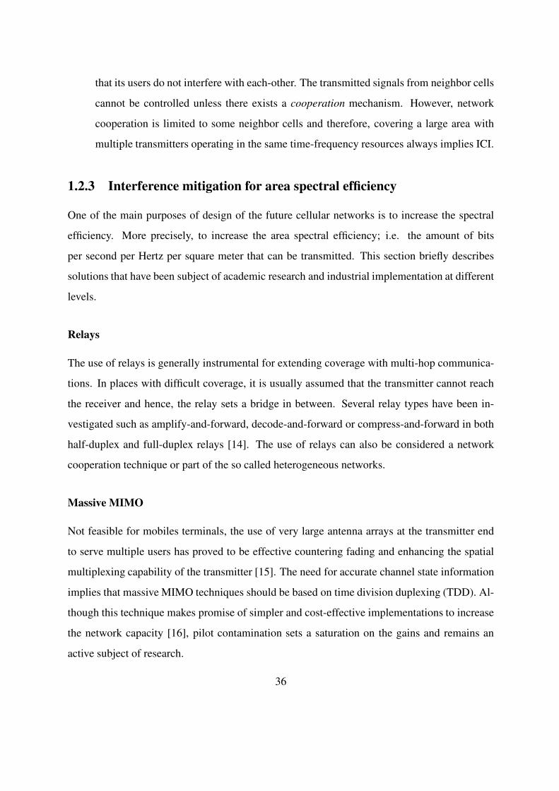
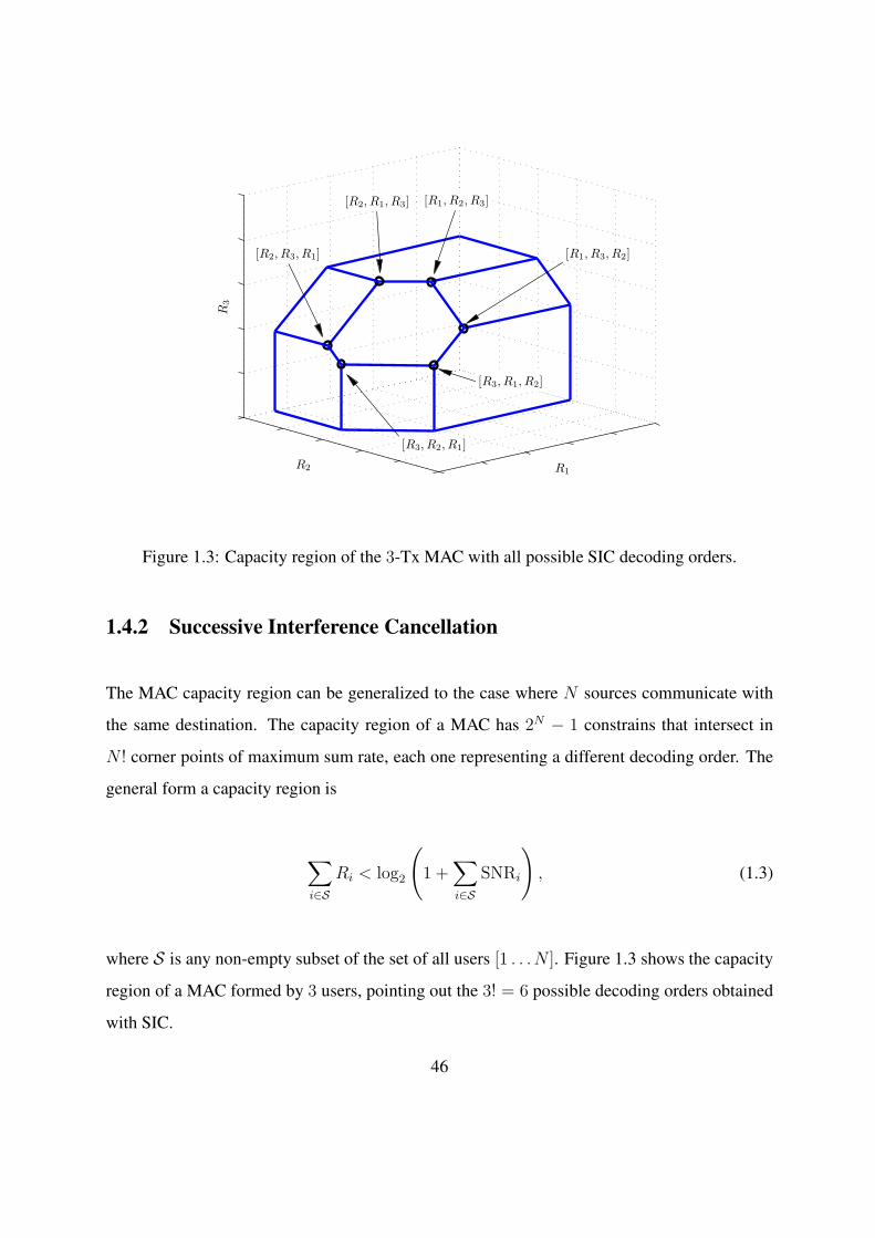
Figure 1.3: Capacity region of the 3-Tx MAC with all possible SIC decoding orders.

1.4.2 Successive Interference Cancellation

The MAC capacity region can be generalized to the case where N sources communicate with

the same destination. The capacity region of a MAC has 2N − 1 constrains that intersect in

N ! corner points of maximum sum rate, each one representing a different decoding order. The

general form a capacity region is

∑

i∈S

Ri < log2

(

1 +∑

i∈S

SNRi

)

, (1.3)

where S is any non-empty subset of the set of all users [1 . . .N ]. Figure 1.3 shows the capacity

region of a MAC formed by 3 users, pointing out the 3! = 6 possible decoding orders obtained

with SIC.

46

0 1 2 30

1

2

3

R2

(b/s/

Hz)

R1 (b/s/Hz)

R1 = log2(1 + SNR1)

R1 = log2(1 + SINR1)

SignalInterference

Rx1

Rx2

Tx1

Tx2

R2 = log2(1 + SINR2)

R2 = log2(1 + SNR2)

Figure 1.4: The IC formed in the downlink of two cells is decomposed in two related MACs.

1.4.3 The Interference Channel

If multiple transmitters want to communicate exclusively with a different receiver, the situation

is known as the Interference Channel (IC). The capacity region for the interference channel has

been for years an open problem and is known only for some special cases (cf. [48–50]). The

downlink of cellular networks is an instance of the IC. For the purpose of this thesis, we point

out that the IC can be decomposed in two related MACs as shown in Figure 1.4

The details and deductions obtained from this decomposition are carefully described in

Chapter 4.

47

Part II

Coordinated Multi-Point Transmission

49

Chapter 2

Coordinated Multi-point transmission

with limited feedback and other-cell

interference

Pushed by the exponential traffic growth and the rapidly increasing demand for multimedia

applications, wireless networks are compelled to evolve in order to meet the extraordinary

performance requirements of future broadband networks in terms of spectral efficiency and

coverage. Fundamental results from information theory [23, 51, 52] advocate for network co-

operation as a promising concept, which in the cellular context could help increase multi-cell

spectral efficiency and improve the coverage performance of cell-edge users. Over the last

years, different network cooperation schemes in the uplink and downlink have been extensively

researched [31, 53, 54] to the point that cooperation has transited from a theoretical concept

to many practical techniques [24, 55, 56]. In 3GPP standardization activities, BS cooperation

is referred to as coordinated multi-point transmission (CoMP) and is included in 4G wireless

standards, such as LTE-Advanced.

The scope in this chapter is in downlink CoMP systems with quantized channel direction

and feedback delay. A general theoretical framework is proposed in section 2.2, allowing to

derive closed-form expressions and accurate approximations for the average achievable rates of

51

CoMP systems with QD-CSI. The analysis is based on tools from [34] and characterizes the in-

terplay between delay and number of feedback bits. The impact of QD-CSI on the average sum

rate performance of JT and CBF systems is analyzed in section 2.3. In section 2.4, a multi-mode

transmission (MMT) scheme is presented, enabling to identify the optimal operating regions of

each CoMP scheme depending on the average SNR, the number of feedback bits, the number

of antennas and users served, and delay. This scheme adaptively switches among transmission

modes in order to maximize the sum rate. Furthermore, for analytical tractability, a moment

matching technique is used to approximate the interference distribution and the weighted sums

of chi-squared random variables by Gamma distributions. These approximations are validated

through system level simulations, evaluating different cases of pathloss asymmetry and the ef-

fect of OCI. In section 2.5 a complete review of the outage performance is obtained based on

derived closed-form expressions for the outage probability of QD-CSI CoMP systems. Numer-

ical results in section 2.6 provide design guidelines under which conditions and system operat-

ing parameters, cellular users would experience higher throughput using CoMP as compared to

non-cooperative transmission techniques.

2.1 System Model and Preliminaries

Consider a network of hexagonal cells, in which a cluster of M coordinated BSs, each located

at the center of its cell, is surrounded by a ring of MOCI non-cooperative cells generating OCI.

The total number of BSs in the system isM+MOCI. Each BS hasNt transmit antennas to serve

1 ≤ U ≤ Nt single-antenna receivers over the same time and frequency resources. Users are

placed at different fixed positions anywhere in the cells and distance-dependent attenuation is

considered. User selection is not considered here and the effect of shadowing is left for future

work. Figure 2.1 illustrates an example of the network model, in which around M = 2 and 3

coordinating cells, the external ring of interfering cells has MOCI = 8 and 9 BSs, respectively.

52

Figure 2.1: Network layout withM =MOCI = 3 (left) and SU-JT withM =MOCI = 2 (right).

2.1.1 Transmission modes

Two main cooperative schemes are investigated here: joint transmission and coordinated beam-

forming. In JT, the coordinated BSs exchange and share both data and control channel informa-

tion (CSI) and under perfect CSI, it can provide multiplexing gain up to Nt and power gain of

the order of M(Nt − U + 1). In CBF, only control channel information (CSI) is shared among

BSs to mitigate the interference inside the cooperative cluster. In theory, a spatial multiplex-

ing gain of at most M can be achieved and the power gain is reduced (with respect to JT) to

Nt −M + 1.

For exposition convenience, both schemes are presented below in the absence of OCI, i.e.

MOCI = 0.

• Joint Transmission Mode (JT): In this transmit mode, the same 1 ≤ U ≤ Nt users are

served from each BS.

The received signal for the j-th user at time instant n is given by

yj[n] =M∑

i=1

U∑

u=1

√

θu,ihHj,i[n]wu,i[n]su,i[n] + z[n], (2.1)

53

where hj,i ∈ CNt×1 is the channel vector from the i-th BS to the j-th user, wu,i ∈ CNt×1

is the precoding vector employed by the i-th BS to transmit to the u-th user, and su,i is

the transmitted signal with power constraint E[∑M

i=1 |si|2]

= P . Equal power allocation

is assumed among all BSs and each channel vector consists of i.i.d. complex Gaussian

elements ∼ CN (0, 1) (Rayleigh fading). The distance-dependent path-loss attenuation

from the i-th BS to u-th user is denoted by θu,i = d−αu,i , with du,i being the distance

between the i-th BS and the u-th user and α is the path-loss exponent. The additive white

Gaussian noise (AWGN) is z[n] ∼ CN (0, 1).

When only one user is served by all BSs (U = 1), the scheme is reffered as single-user

joint transmission (SU-JT) and wu,i ∈ CNt×1 is the eigen-beamforming vector used by

the i-th BS for user u, i.e. wu,i = hu,i. For U > 1, the scheme is called multiuser joint

transmission (MU-JT) and wu,i is the zero-forcing precoding vector.

• Coordinated Beamforming (CBF): In this mode, BSs serve different users exploiting

knowledge of the control channel information from neighboring cells. Each BS uses

the shared CSI to serve its own user nulling the interference caused to users from neigh-

boring cells. The received signal at the u-th user served by the u-th BS at instant n is

given by

yu[n] =√

θu,uhHu,u[n]wu[n]su[n] +

M∑

i=1i 6=u

√

θu,ihHu,i[n]wi[n]si[n] + z[n]. (2.2)

For CBF, this thesis considers always U = M and wu is the u-th column of the zero-forcing

beam-forming matrix (Moore-Penrose pseudoinverse).

2.1.2 Imperfect CSI

• Delay CSI feedback: The standard Gauss-Markov regular process is used to study the ef-

fect of CSI delay and to model the temporal variation of the channel state. A block fading

model [57] is assumed, where h remains constant over each frame of length T channel

uses, and evolves from frame to frame according to an ergodic stationary spatially white

54

jointly Gaussian process. Under the Gauss-Markov AR(1) model (i.e., auto regressive of

order 1), the channel evolves in time as

h[n] = ρh[n − 1] + e[n], (2.3)

where ρ is the correlation coefficient (0 < ρ < 1), h[n] denotes the channel realization at

time instant n and the error vector e[n] ∈ CNt×1 is complex Gaussian with zero mean and

variance ǫ2 = 1− ρ2 (i.i.d. in time and independent of h[n− 1]). For the channel correla-

tion coefficient, we use the Jakes-Clarke’s model and set ρ = J0(2πfdTs), where J0(·) is

the zero-th order Bessel function of the first kind, fd denotes the Doppler frequency shift

and Ts the symbol time. Note that channel estimation or prediction errors can be also

modeled using the above auto-regressive model, making these results more general.

• Quantized CSI: In FDD systems, each user reports back to its BS channel direction in-

formation (CDI) for the channels between the user and its serving and interfering BSs.

This is done using a quantization codebook known at both sides. Each user employs

a different codebook and the quantized channel is chosen from a codebook denoted by

Cu = cu,1, cu,2, . . . , cu,L and containing L = 2b unit norm vectors. The chosen quan-

tization codevector is the one maximizing |hHu,icu,ℓi| and the index ℓi is fed back using b

bits at BS i, where hu,i =hu,i

‖hu,i‖is the CDI. This criterion is equivalent to minimizing the

quantization error sin2 φ = 1 − |hhH |2 where h = cu,ℓi is the quantized channel direc-

tion. Since it provides a good compromise between analytical tractability and asymptotic

optimality [33,58], random vector quantization (RVQ) is used. The expected value of the

cosine of the angle φ = ∠hh, which is related to the quantization error, is given by [59]

ξ = Eφ

[cos2 φ

]= 1− 2b · β

(

2b,Nt

Nt − 1

)

, (2.4)

where β(·, ·) is the Euler Beta function.

2.1.3 Preliminaries

Consider a heterogeneous scenario with unequal path-loss and Rayleigh fading, hence terms

(signal, interference, or OCI) involving sums of χ2 distributed random variables appear. Those

55

sums become weighted sums of χ2 variates due to different distances between users and BSs.

Notice that a chi-squared distribution is a special case of the Gamma distribution, such that if

aX ∼ χ2(D), aX = A, then A ∼ Gamma(D, a), where D is the shape parameter and a is the

scale parameter.

Exact Results

Let Ai ∼ Gamma(Di, θi) and X =∑M

i=1Ai. There are various closed-form solutions for the

distribution ofX [60,61]. The sums of Gamma random variables have scale parameters Di ∈ N

and different θi > 0. In this case, the exact distribution for the sum of Gamma distributed r.v. is

given by [62]

fX (x) = K

M∑

i=1

Pi (x) e−θix, (2.5)

where

K =

M∏

i=1

θDi

i , Pi (x) =

Di∑

k=1

ci,kxk−1,

ci,Di=

1

(Di − 1)!

M∏

j=1j 6=i

(1

θj−

1

θi

)−Dj

, i = 1, . . . ,M, (2.6)

and

ci,Di−k=

1

k

k∑

j=1

(Di − k + j − 1)!

(Di − k − 1)!R (j, i,M) ci,Di

, k = 1, . . . , Di − 1, i = 1, . . . ,M,

R (j, i,M) =M∑

k=1k 6=i

Dk

(1

θi−

1

θk

)−j

, j = 1, . . . , Di − 1. (2.7)

Approximate Results

One of the objectives of this work is to derive closed-form expressions for the achievable sum

rate in CoMP systems, for which the pdf of the SINR distribution should be kept as simple as

possible so that E[log2(1 + SINR)] can be reduced to an insightful expression. Using (2.5) in

any of the SINR terms makes the expression for the achievable throughput intractable. For that,

advantage is taken of the fact that the weighted sum of gamma distributions can be very well

56

approximated with another gamma distribution, and the precision of this approximation depends

on the similarity of the scales of the different terms in the sum, i.e. the different distances

from BSs to mobile users. The distribution of X =∑M

I=1Ai with Ai ∼ Gamma(Di, θi) is

approximated by a Gamma distribution by matching the first two moments (moment matching

method). In other words, X is approximated by a Gamma distributed r.v. X such that the first

and second moments of X , µX = DX θX and σ2X = DX θ

2X , respectively, are equal to the sum

of all first and second moments of every Ai respectively, i.e.

µX = DX θX =M∑

i=1

Diθi, σ2X = DX θ

2X =

M∑

i=1

Diθ2i .

Therefore, to find the scale and shape parameters for X , one only needs to calculate

DX = fD(D, θ

)=

(∑M

i=1Diθi

)2

∑Mi=1Diθ2i

, θX = fθ(D, θ

)=

∑Mi=1Diθ

2i

∑Mi=1Diθi

, (2.8)

where D = [D1 . . .DM ] and θ = [θ1 . . . θM ]. (·) is used to denote a second order approx-

imation of a Gamma distributed r.v. and fD (·, ·) , fθ (·, ·) are the functions to find the shape D

(DoF in the equivalent χ2 distribution) and scale θ parameters respectively. Consequently, the

r.v. X ∼ Gamma(DX , θX) is said to be a second order approximation of X using the moment

matching method.

2.2 Average Achievable Rate Analysis

This section provides an analytic framework to calculate the average achievable rate for both JT

and CBF CoMP transmissions. Considering the general case where the effect of quantization

and delay on the CSI, the inherent unequal pathloss attenuations, and the impact of OCI are all

included. First, we start by deriving the distribution of the SINR, which serves as a building

block for calculating the average rate.

57

2.2.1 SINR Distribution in JT

The case of MU-JT is revised, deriving the distributions of the and interference signals as a

means to calculate the SINR distribution.

Desired Signal

The desired signal for the u-th user at instant n is received from M BSs and takes on the form

SJT,u =P

MU

M∑

i=1

θu,i∣∣hH

u,i[n]wu,i[n]∣∣2. (2.9)

Under the QD-CSI model used in this paper and described in Section II, the expression can

be expanded and then simplified as shown in the following proposition.

Proposition 1. In a JT system, the desired signal for the u-th user at instant n under quantized

and delayed CSI is given by

S(qd)JT,u =

Constant︷︸︸︷

Pρ2ξ

MU

M∑

i=1

θu,i

Gamma r.v.︷︸︸︷

‖hu,i[n− 1]‖2∣∣∣h

Hu,i[n− 1]wqd

u,i[n]∣∣∣

2

∼Pρ2ξθ

MUX ∼ γxX,

where all constant terms can be grouped in γx = Pρ2ξθ/MU with θ = fθ (Nt, [θu,1 . . . θu,M ]),

ξ is given in (2.4), and the r.v. is X ∼ Gamma(D, 1), with D = fD (Nt, [θu,1 . . . θu,M ]).

Proof. See Appendix A.0.2.

Interference Term

Under quantized and delayed CSI and U > 1, interference is created in the downlink transmis-

sion within the cooperative cluster. The interference generated from M BSs is given by

I(qd)JT,u =

P

MU

M∑

i=1

θu,i

U∑

j 6=u

∣∣∣h

Hu,i [n]w

qdu,j [n]

∣∣∣

2

. (2.10)

Aiming to calculate the achievable rate, we simplify (2.10) in the following proposition.

58

Proposition 2. In a JT system, the inter-cell interference term for the u-th user at instant n

under quantized and delayed CSI is distributed as

I(qd)JT,u ∼

P

MU

M∑

i=1

θu,i[ρ2δY1 + ǫ2Y2

]

≈ γy1Y1 + γy2 Y2, (2.11)

where γy1 = Pρ2δθ/MU , γy2 = Pǫ2θ/MU , θ = fθ(U − 1, [θu,1 . . . θu,M ]), ρ and ǫ are given in

(2.3), and δ = 2−b/(Nt−1). Both Y1, Y2 ∼ Gamma(D, 1) and D = fD(U − 1, [θu,1 . . . θu,M ]).


2.2.2 SINR Distribution in CBF

Considering now the case of CBF and the distribution of the desired signal and the interference

term are derived accordingly.

Desired Signal

In CBF case, the desired signal arrives at the receiver from only one BS, thus eliminating the

summation in (2.10) and having only one pathloss attenuation coefficient θu,u in front. In that

case, similarly to Proposition 1, the desired signal is given by

SCBF,u =Pρ2ξ

Mθu,u ‖hu,u[n− 1]‖2

∣∣∣h

Hu,u[n− 1]wqd

u,u[n]∣∣∣

2

∼ γxX, (2.12)

where γx = Pρ2ξθu,u/M and X ∼ Gamma(Nt −M + 1, 1).

Interference term

The interference in the CBF case is the summation of M − 1 terms coming from M − 1 BSs

serving one user each. Hence, the result in 2.10 can be rewritten as

I(qd)CBF,u =

P

MU

M∑

i=1i 6=u

θu,i

∣∣∣h

Hu,i [n]w

qdu,j [n]

∣∣∣

2

. (2.13)

59

Following the same derivations as in the JT case (see Appendix A.0.3), the distribution of I(qd)CBF,u

is given by

I(qd)CBF,u ∼

P

M

M∑

i=1i 6=u

θu,i[ρ2δY1 + ǫ2Y2

]

≈ γy1Y1 + γy2Y2, (2.14)

where now γy1 = Pρ2δθ/M , γy2 = Pǫ2θ/M , θ = fθ(1, [θu,1 . . . θu,i−1, θu,i+1 . . . θu,M ]). Both

Y1, Y2 ∼ Gamma(D, 1) and D = fD(1, [θu,1 . . . θu,i−1, θu,i+1 . . . θu,M ]).

2.2.3 The effect of Other-Cell Interference

Considering MOCI non-cooperative (interfering) cells and that each interfering BS transmits

one single stream under the same power constraint per BS, the OCI term is given by the

weighted sum of MOCI gamma distributed random variables. Evidently, the pathloss attenu-

ation is larger in the case of OCI than for the signals generated inside the cooperative cells, as

the users to serve are expected to be near the cell edge. The OCI, which is considered to be the

same for any transmission mode, is given by

OCI =P

M

MOCI∑

i=1

θu,i |hu,iwi|2

∼ γy3Y3, (2.15)

where γy3 = P θOCI/M and Y3 ∼ Gamma(D, 1). In this case, the gamma approximation can

be used as

D = fD (1, [θu,OCI1, . . . , θu,MOCI]) , and θOCI = fθ(1, [θu,OCI1, . . . , θu,MOCI

]).

2.2.4 General Expressions for Average Achievable Rate

In this section, a general result is given for the average achievable rate for a general expression

of SINR given as ratio of gamma distributions. This general SINR expression incorporates the

60

DoF of X DoF of Y1 DoF of Y2

γx DX γy1 γy2 DY1 DY2

CBF Pρ2ξθ/M Nt − U + 1 Pρ2δθ/M Pǫ2θ/M U − 1 U − 1

JT Pρ2ξθ/MU M(Nt − U + 1) Pρ2δθ/MU Pǫ2θ/MU M(U − 1) M(U − 1)

Table 2.1: Variables and values for CBF and JT

SINR of any of the aforementioned CoMP transmission schemes and takes on the form of

SINR(qd)CoMP,u =

γxX

1 + γy1Y1 + γy2Y2 + γy3Y3, (2.16)

where (qd) implies QD-CSI. This SINR expression takes a particular form for different CoMP

schemes depending on the values of the parameters of the gamma distributed random variables,

as given in table 2.1.

In both CBF and JT cases, γy3 = PθOCI/M and for the gamma distribution Y3, DY3 =

MOCI . The values shown in Table 2.1 do not consider unequal pathloss. In the heterogeneous

scenario with unequal path-loss, an approximate SINR expression is used where the parameters

θ and D are replaced by the corresponding values obtained using the Gamma approximation as

θ = fθ(D, θ) and D = fD(D, θ) according to (2.8).

Based on (2.16), a general expression for the average achievable per-user rate, which is valid

for both CBF and JT is derived.

Theorem 1. In JT and CBF systems with quantized and delayed CSI and OCI, the average

achievable per-user rate is approximated by

R(qd)CoMP,u ≈ log2 (e)

DX−1∑

i=0

3∑

j=1

DYj−1

∑

k=0

i∑

l=0

κ(j)k (l + k)!

l! (i− l)!γl+k−i+1x

I

(1

γx,γxγyj

, i, l + k + 1

)

, (2.17)

where

I (a, b,m, n) =

∫ ∞

0

xme−ax

(x+ b)n (x+ 1)dx. (2.18)


61

The achievable rate expression can be simplified in the high SNR regime (interference-

limited region), in which SINR(qd)CoMP,u ≈ γxX/(γy1Y1 + γy2Y2 + γy3Y3).

Corollary 1. In the high SNR regime, the average achievable per-user rate of JT and CBF

systems with quantized and delayed CSI and OCI is approximated by

R(qd,h−SNR)CoMP,u ≈ log2 (e)

DX−1∑

i=0

3∑

j=1

DYj−1

∑

k=0

κ(j)k (i+ k)!

i!ak+1I2

(γxγyj

, i, i+ k + 1

)

, (2.19)

where

I2 (a,m, n) =

∫ ∞

0

xm

(x+ a)n (x+ 1)dx.


2.2.5 Special Case: Single User JT

In this subsection, single-user JT systems is examined, i.e. JT mode where only one user is

served, and provide simpler expressions for the average achievable rate. Since only one user is

served, there is no interference coming from the cooperative cluster, and the SINR takes on the

form γxX/(1 + γy3Y3).

Corollary 2. In single-user JT systems with quantized and delayed CSI, the average achievable

rate is approximated as

R(qd)SUJT ≈ log2 (e)

DX−1∑

i=0

i∑

j=0

(DY3 + j − 1)!γDY3

+j−ix

j! (i− j)! (γy3 − 1)!γDY3y3

× I

(1

γx,γxγy3

, i, DY3 + j

)

.(2.20)

Proof. The result follows easily by applying the same derivations shown in Appendix A.0.4

and using the pdf of Y3 in Appendix A.0.4 equation (A.5).

Furthermore, the following simpler expression can be obtained in the high SNR regime.

Corollary 3. In the high SNR regime, the average achievable rate in single-user JT systems

with quantized and delayed CSI is approximately given by

R(qd,h−SNR)SUJT ≈ log2 (e)

DX−1∑

i=0

(DY3 − 1 + i)!

i! (γy3 − 1)!

(γxγy3

)DY3

× I2

(γxγy3

, i, DY3 + i

)

.(2.21)

62

Proof. The result follows easily from Corollary 2 and applying the same steps as in appendix

A.0.5.

In the absence of OCI, e.g. due to orthogonal frequency allocation among cells, the SINR

is given by SINR = γxX and the achievable rate is given by [63]

Rqd,noOCISUJT ≈ log2 (e) e

1/γx

DX−1∑

i=0

Γ (−i, 1/γx)

γix, (2.22)

where Γ(α, x) =∫∞

xtα−1e−t dt is the lower incomplete gamma function.

2.3 Rate Degradation due to Quantization and Delay

In this section, the impact of quantization and delay on the average achievable rate in CoMP

systems is investigated. It is also shown that if the feedback rate is scaled at the appropriate

rate, a constant rate offset between the rate achievable with perfect CSI and that with QD-CSI

can be maintained.

2.3.1 Quantization

First, the effect of delay is neglected and only quantized CSI is considered using RVQ. In that

case, the per-user average rate loss is upper bounded as

∆R(q)u = RCoMP,u − R

(q)CoMP,u = E log2 (1 + SNRu) − E log2 (1 + SINRu)

≤ log2

(

1 +P θ (U − 1)

U2− b

Nt−1

)

, (2.23)

where for CBF, in the denominator of the above expression U =M and for U = 1, ∆R(q)u = 0.

The following proposition gives a sufficient scaling of feedback bits to maintain a constant

bounded rate offset.

Proposition 3. To maintain a constant rate offset per-user of log2(β) between CoMP with per-

63

fect CSI and with quantized CSI, the number of feedback bits per user should scale as

b = (Nt − 1) log2

(

P θ(U − 1)

U

)

− (Nt − 1) log2 (β) (2.24)

≈ (Nt − 1)PdB + (Nt − 1) log2

(

θ(U − 1)

U

)

− (Nt − 1) log2 (β) (2.25)

Proof. The result follows by setting the rate offset upper bound given in (2.23) equal to the

maximum allowable gap of log2 b and solving for b. The approximation comes from the fact

that log2 P ≈ PdB/3. Note that the above result is in accordance with results in [33] for multi-

user MISO broadcast channels with quantized CSI.

2.3.2 Delay

The average rate offset is considered when only delayed CSI is taken into account. Similarly to

the case of quantized CSI and (2.23), the following rate offset upper bound due to delayed CSI

is given

∆R(d)u ≤ log2

(

1 +P θ (U − 1)

Uǫ2

)

. (2.26)

Since ǫ2 = 1 − ρ2 is related to the Bessel function of the first kind, we notice that for realistic

values, the product 2πfdTs < 1 and so we can simplify the value of ǫ2 with relative good

precision as

ǫ2 = 1− J20 (2πfdTs) = 1−

∞∑

i=0

(−(2πfdTs)

2

4

)i

(i!)2

2

= 1−

[1∑

i=0

− (πfdTs)2i

(i!)2−O((πfdTs)

4)

]2

≈ 1−

(

1−(πfdTs)

2

4

)2

≈ 2 (πfdTs)2 . (2.27)

In order to maintain a constant rate offset no larger than log2(β), let

log2

(

1 +P θ (U − 1)

Uǫ2

)

= log2(β). (2.28)

64

Replacing (2.27) into (2.28) and solving for Ts, the following result is obtained

Ts =1

πfd

√

U (β − 1)

2P θ (U − 1). (2.29)

This result shows a non-linear relation between the maximum delay on the feedback and the

rate offset, as Ts should scale in the order of P−1/2.

2.3.3 Quantization and Delay trade off

If the effect of both quantization and delay is taken into account, the average rate offset can be

derived similarly to [13] as

∆R(qd)u ≤ log2

(

1 +P θ (U − 1)

U

[ρ2δ + ǫ2

]

)

, (2.30)

where δ = 2−b/(Nt−1).

In order to maintain a bounded rate offset no larger than log2(β), the number of feedback

bits per user and the delay spread should scale as

b = (Nt − 1) log2

(

ρ2(U − 1)P θ

U(β − 1)− ǫ2P θ(U − 1)

)

(2.31)

Ts =1

πfd

√

U (β − 1)

2P θ (U − 1) (1− δ)−

δ

2(1− δ). (2.32)

The tradeoff between delay and feedback resolution is shown in Figure 2.2 for ǫ2 ≈ δ ≈ 0.2,

Ts = 5 ms, and b = 7 bits. In this setting, a rate loss of 1 bps/Hz can be seen by either reducing

by 2 bits the feedback resolution or increasing the delay by 4 ms.

2.4 Adaptive Multi-mode Transmission

In the previous average achievable rate analysis, it was shown that under imperfect CSI, there is

a tradeoff between different CoMP transmission modes, i.e. CBF, SU-JT, and MU-JT, and the

natural question that arises is which CoMP modes is optimal to use in each case. A crisp theo-

retical answer to this question seems to be hard to give as the optimal CoMP scheme depends on

65

2 4 6 8 10 124

4.5

5

5.5

6

6.5

7

7.5

8

8.5

9

# bits/CSI

Rate

loss (

bps/H

z)

per User ∆R vs Feedback resolution

0 2 4 6 8 104

4.5

5

5.5

6

6.5

7

7.5

8

8.5

9

Ts (ms)

Rate

loss (

bps/H

z)

per User ∆R vs Delay

b = [2, 4, 8, 12] b/CSI

Ts = [0.5, 3.5, 6.5, 9.5] ms

Figure 2.2: Average per user rate offset for CBF with perfect and QD-CSI in the high SNR

regime (i.e. SNR = 30 dB) for M = 2, Nt = 4, v = 5 km/h, and fc = 2.1 GHz.

many parameters, namely path-loss, SNR operating regime, feedback resolution, delay, number

of users, BSs, and antennas. For that, a set of simple rules is provided, based on the closed-

form expressions and an adaptive multi-mode transmission scheme is proposed. In this policy,

the achievable sum rate can be maximized by adaptively switching among different transmis-

sion modes (SU-JT, MU-JT, and CBF) as a means to balance between power gain and spatial

multiplexing gain. Under MMT, the active transmission mode m∗ is selected as

m∗ = argmaxm

R(m) (2.33)

where

R(m) =

∑Mu=1R

(qd)CBF : m = 0

∑Uu=1R

(qd)JT,u : m = U

To build further intuition, an approximate framework in order to analytically find the switch-

ing points for the proposed MMT scheme is presented. For that, expressions for the difference

between the rates of different CoMP modes along all SNR regimes were found. Following

66

previous notation, the rate difference is in general defined as

∆R := R− R′ = UE

log2

(

1 +aX

1 +∑

i biYi

)

− U ′E

log2

(

1 +a′X ′

1 +∑

i b′iY

′i

)

.

(2.34)

Proposition 4. In the low to moderate SNR regime, the rate difference between two CoMP

transmission modes without OCI is approximated by

∆R(mod.SNR) ≈ log2

( (aeUψ(DX)

)

(a′eU ′ψ(DX′))

)

, (2.35)

where ψ(·) is the digamma function.


Proposition 5. In the high SNR regime, the rate difference between two CoMP transmission

modes without OCI is approximated by

∆R(high SNR) ≈ log2

( [ηeψ(DX)−ψ(DY )

]U

[η′eψ(DX′ )−ψ(DY ′)]U ′

)

, (2.36)

where η is defined in Appendix A.0.7.


Tighter approximations can be obtained by defining the following rate differences

∆R1 := R(qd)SUJT − R

(qd)MUJT (2.37)

∆R2 := R(qd)SUJT − R

(qd)CBF. (2.38)

Using these rate differences and based on Propositions 4 and 5 the following corollaries are

obtained as indicated in [63].

Corollary 4. In the low to moderate SNR regime, the rate difference between SU mode and MU

mode in JT and CBF transmission is approximated by

∆R1 = ∆R2 ≈ log2

(

1 + aDX

(a′eψ(DX′))U ′

)

. (2.39)

67

Proof. The proof follows easily along with the elements of Appendix A.0.6 replacing R(1) =

R(qd)JT,1 and R′(U) =

∑Uu R

(qd)JT,u for ∆R1 and R′(0) = R

(qd)CBF for ∆R2.

Corollary 5. In the high SNR regime, the rate gap between between SU mode and MU mode in

JT and CBF transmission is

∆R1 = ∆R2 ≈ log2

(

aDX

[η′e(ψ(DX′)−ψ(DY ′ ))]U ′

)

. (2.40)

Proof. The proof is based on Appendix A.0.7, replacing R(1) = R(qd)JT,1 and R′(U) =

∑Uu R

(qd)JT,u

for ∆R1 and R′(0) = R(qd)CBF for ∆R2.

In the presence of OCI, the above approximations become looser, the reason being the inclu-

sion of additional gamma distributions with different scale and shape parameters. In Figure 2.3,

the rate differences obtained with the analytic framework derived in section 2.2.4 are shown on

the upper graph. In the bottom, the approximations for ∆R indicate a minor shift of the order

of 2− 3 dB for both high and moderate SNR regimes.

2.5 Success Probability Analysis

As shown in the previous sections, the SINR for the main CoMP transmission modes, can be

written as the ratio of gamma functions (2.16). This result gives the possibility of deriving the

success probability for each case, analyzing how the different modes and the analytic approxi-

mations impact the performance. The success probability is defined as the probability that the

received SINR at the u-th user, is greater than a predefined threshold β; or equivalently, the

probability that the user is not in outage, i.e.:

P(u)succ = 1− P

(u)out

= 1− P SINRu ≤ β

= 1− FSINRu(β), (2.41)

where FSINRuis the CDF of the random variable SINRu.

68

−5 0 5 10 15 20 25 30 35 400

5

10

15Adaptive Multi−Mode Transmission

SNR (dB)

Su

m R

ate

(b

ps/H

z)

JT, U = 1

JT, U = 2

JT, U = 3

CBF

−5 0 5 10 15 20 25 30 350

5

10

15

SNR (dB)

Su

m R

ate

(b

ps/H

z)

JT, U = 1

JT, U = 2

∆ R1

Approx ∆R1

h−SNR

JT, U = 2 JT, U = 3

Crossing pointsapproximations

JT, U = 1CBF

Figure 2.3: Top: Adaptive Multi-mode Transmission for CoMP. M = 3, Nt = 4 and b = 4.

Bottom: ∆R approximations and crossing points. M = 3, Nt = 2 and b = 6. Both graphs use

v = 5 km/h, Ts = 1 ms, and fc = 2.1 GHz.

2.5.1 Single User Joint Transmission

Starting from the simplest case, the SINR for a single user served on JT by M stations is

SINR = γx∑M

i=1Xi, where Xi ∼ Gamma(Nt, θi). Accordingly, the expression for the CDF

of the sum of multiple Gamma distributed r.v. is used in order to write the success probability

as

P(u)succ = 1− FSINRu

(β)

= KM∑

i=1

P ∗i (β)e

−β/θi, (2.42)

69

where

K =

M∏

i=1

1/θDi

i , P ∗i (x) =

Di∑

k=1

ci,k(k − 1)!

k−1∑

j=0

θk−ji xj

j!,

ci,Di=

1

(Di − 1)!

M∏

j=1j 6=i

(1

θj−

1

θi

)−Dj

, i = 1, . . . ,M,

and

ci,Di−k=

1

k

k∑

j=1

(Di − k + j − 1)!

(Di − k − 1)!R (j, i,M) ci,Di−(k−j),

k = 1, . . . , Di − 1, i = 1, . . . ,M,

R (j, i,M) =

M∑

k=1k 6=i

Dk

(1

θi−

1

θk

)−j

, j = 1, . . . , Di − 1.

If the SINR includes any exact distribution of sums of Gamma random variables the success

probability expression is intractable. It is possible to appeal to the moment matching approxi-

mation proposed in (2.8).

SU-JT without Interference

Finding a good approximation for the sum of Gamma r.v. as X ≈∑M

i=1Xi where X ∼

Gamma(D, Nt), facilitates the analysis because SINR = γxX and the success probability is

easily obtained as

P(u)succ = e−β/θX

DX−1∑

i=0

(

β/θX

)i

i!. (2.43)

SU-JT with OCI

If OCI is taken into account, based on SINR = θXX/(1 + θY Y ), where θY Y represents the

OCI, following the proof in A.0.8 then (2.43) is simplified as


DX−1

∑

i=0

i∑

j=0

(i

j

)(β/θX)

i

i!

∂jLY (β/θX)

∂ (β/θX)j , (2.44)

70

where

∂jLY (β/θX)

∂ (β/θX)j = (−θY )

j (DY − 1 + j)!

(DY − 1)!

(

1 +θYθXβ

)−DY−j

as shown in (2.50).

SU-JT high-SNR regime

In the high-SNR regime, where the system is interference limited, the Gamma approximation

yields a simpler expression: SINR = θXX/(θY Y ) and the success probability is


DX−1

∑

i=0

(β/θX)i

i!

∂iLY (β/θX)

∂ (β/θX)i . (2.45)

2.5.2 Multi-user CoMP modes

Based on the single-user case in (2.43), the analysis for any CoMP transmission mode serving

multiple users is extended; either for MU-JT or CBF.

Success Probability for multi-user CoMP

As shown in section 2.2 in the more general case withM cooperative BSs and MOCI interfering

BSs the SINR =∑M

j=0 θjXj/(1+∑MOCI

k=1 = θkYk). Using a Gamma approximation only on the

signal term SINR = θXX/(1 +∑MI

k=1 = θkYk), the following result on the success probability

is obtained.

Theorem 2. The success probability under CoMP with QD-CSI and OCI, in which the u-th

user is served by M BSs and receives interference from MOCI BSs, is given by


DX−1

∑

i=0

i∑

j=0

(i

j

)(β/θX)

i

i!

∂j∏MOCI

k=1 LYk (β/θX)

∂ (β/θX)j , (2.46)

where LYk is the Laplace transform of each interfering term.


71

Simplified Success Probability for multi-user CoMP

The above result may not be easy to calculate as one needs to find high-order derivatives of the

product of MI Laplace transforms. In both CBF and MU-JT, the most important interference

terms are due to quantization and OCI. Hence to provide a simpler expression, the delayed CSI

term is neglected and the SINR takes the form SINR = X/(1 + Y1 + Y2).

Theorem 3. The success probability under CoMP with Q-CSI and OCI, in which the u-th user

is served byM BSs and receives interference fromMOCI BSs, is given by the success probability

for a multi-user CoMP transmission and can be written as

P(u)succ = e−s

DX−1

∑

i=0

i∑

j=0

j∑

k=0

si

i!

(i

j

)(j

k

)

LY1(s)(j−k)LY2(s)

(k), (2.47)

where LY1(s)(j) is the j-th derivative of the Laplace transform of Y1(s).


Moment Generating functions

As stated previously, the Laplace transform can be calculated by means of the MGF. For any

Gamma distributed random variable X ∼ Gamma(D, θ), the MGF is MX(x) = (1 − xθ)−D

and therefore

LX(x) =MX(−x) = (1 + xθ)−D. (2.48)

For each of the interference terms Yi ∼ Gamma(DYi, θYi) the (zero order derivative) Laplace

transform is

L(0)Yi(β/θX) =

(

1 +θYiθXβ

)−DYi

. (2.49)

The j-th derivative is obtained as

L(j)Yi(β/θX) = θj

Yi(−DYi

)(−DYi− 1) . . . (−DYi

− j + 1)

(

1 +θYiθXβ

)−DYi−j

= (−θYi)j(DYi

)(DYi+ 1) . . . (DYi

+ j − 1)

(

1 +θYiθXβ

)−DYi−j

= (−θYi)j(DYi

+ j − 1)!

(DYi− 1)!

(

1 +θYiθXβ

)−DYi−j

(2.50)

72

0 10 20 300

5

10

15

Tx SNR (dB)

Su

m R

ate

(b

ps/H

z)

0 10 20 300

5

10

15

Tx SNR (dB)

Su

m R

ate

(b

ps/H

z)

JT, U = 1

JT, U = 2

JT, U = 4

Analytic

Simulation

CBF, U = 2,perfect CSI

+OCIloss

QD−CSIloss

QD−CSIloss

Figure 2.4: Left: Achievable rates for JT with perfect and QD-CSI. M = 3, Nt = 4, b = 10,

and v = 10 km/h. Right: Achievable rates for CBF including perfect CSI, QD-CSI and the

effect of OCI. M = 2, Nt = 4, b = 8, and v = 5 km/h.

the above results may finally be used to evaluate the system performance in terms of the

so called transmission capacity [64] or equivalently the spectral efficiency of a transmission

scheme that operates with no link adaptation mechanism, supposing the use of capacity achiev-

ing coding and modulation. A system with U users has a transmission capacity in the form

C =U∑

u=1

log (1 + βu)P(u)succ (2.51)

2.6 Numerical Results

In this section, the performance analysis and the analytical expressions and approximations de-

rived in Section 2.2.4 are validated. First, the approximation for the achievable rate with equal

pathloss (homogeneous scenario) is verified. Unless otherwise stated, Ts = 1 ms and fc = 2.1

GHz. In Figure 2.4, the analytical expressions derived above with simulations are compared.

The graph on the left shows the number of users U served in JT to maximize the sum rate for

73

an increasing SNR, however the achievable sum rate of MU-JT exhibits a ceiling effect due

to imperfect CSI. On the right-hand graph, a similar result is obtained for CBF, showing the

significant impact of quantization and delay on the sum rate, while OCI reduces the sum rate

by almost 50% in the high SNR regime. Second, in Figure 2.5, the gamma distribution ap-

proximations considered in the heterogeneous scenario with unequal pathloss are verified. Its

is observed that the analytical expressions, which also use the moment matching approxima-

tion method, provide an accurate approximation in all cases, i.e. CoMP with QD-CSI when

approximations are taken on the signal and interference terms, and CoMP with OCI where an

additional approximation is used in the denominator of the SINR. The figure also shows the

rate degradation due to quantization and delay and the additional degradation incurred for OCI.

Moreover, in Figure 2.6, the results based on RVQ are compared with the performance using

standardized LTE codebooks [65] for CBF without OCI. As expected, if the number of antennas

(or BSs) increase, RVQ exhibits a performance very close to codebooks used in real systems.

In Figure 2.7, it is shown the number of feedback bits required to obtain a rate gain by

adding one more BS in the cooperative cluster no larger than 0.5 bps/Hz for different CoMP

modes. It can be observed that adding a BS in the cooperative cluster, e.g. going from 2 to 3

BSs, requires a feedback rate of around 7 bits per user per BS, which is larger that the resolution

used in current LTE systems.

Furthermore, the case when it is beneficial from an average sum rate point of view to perform

CoMP transmission as compared to a non-cooperative transmission is evaluated. In the latter,

it is assumed that each of M BSs transmits independently to its user using eigen-beamforming

(also known as maximal ratio combining at the transmitter (MRT)). Determining whether CoMP

transmission is beneficial is dominated by the distance (path-loss) of the user(s) to the possible

CoMP BSs. In Figure 2.8, it is seen that as the feedback resolution increases, the region where

CoMP outperforms MRT is extended. If a set of users is placed in any point inside that region,

the respective CoMP mode under QD-CSI and OCI performs better than MRT under the same

operating conditions. If all users are outside the region, performing non-cooperative transmis-

sion achieves higher sum rate compared to CoMP. We also see that CBF has a broader region

than JT, however in terms of sum rate, JT has larger gains over MRT than CBF. Finally, for

74

−5 0 5 10 15 20 25 300

1

2

3

4

5

6

7

Tx SNR (dB)

Su

m R

ate

(b

ps/H

z)

Gamma Approximation

Simulation

Gamma Approximation

Simulation

QD−CSI + OCISU−JT

QD−CSI + OCICBF

QD−CSICBF

Figure 2.5: Gamma approximations on the signal term, the interference terms and the OCI term.

Users are randomly placed around the cell-edge. M = 2, Nt = 4, b = 4 bits.

M = 3 and b = 4, there is no cell area in the cluster for which CoMP is beneficial.

The performance of the different transmission modes compared to MRT for 2 BSs having 4

antennas is shown in Figure 2.9. Different feedback resolution and delay values are evaluated

as the SNR increases. Both users have been placed near the cell-edge. MU-JT is not shown

as its results are only marginally better than CBF which does not implies sharing data among

BSs. In the low SNR regime, MRT dominates both graphics. SU-JT is the best mode for low

feedback resolution, but the addition of OCI gives to CBF a wider region over SU-JT. Finally

CBF provides superior performance in a large portion of both graphics but important gains are

seen only from the medium resolution, low delay and medium SNR regimes combined.

75

0 5 10 15 20 25 30 351

2

3

4

5

6

7RVQ vs LTE codebook

Tx SNR (dB)

Su

m R

ate

(b

ps/H

z)

LTE codebook

RVQ codebook

Nt = b = 4

Nt = b = 2

Figure 2.6: Average Sum Rate of CBF systems without OCI for M = 2, Nt = 4, and v = 5

km/h.

76

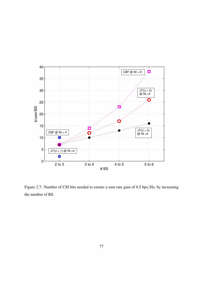
2 to 3 3 to 4 4 to 5 5 to 60

5

10

15

20

25

30

35

40

# BS

b/u

se

r/B

S

CBF @ Nt = 8

CBF @ Nt = 4

JT(U = 1) @ Nt =4

JT(U = 3)@ Nt =4

JT(U = 2)@ Nt =4

Figure 2.7: Number of CSI bits needed to ensure a sum rate gain of 0.5 bps/Hz, by increasing

the number of BS.

77

−500 0 500

−600

−300

0

300

600

d (m)

d (

m)

JT (U=2)

−500 0 500

−600

−300

0

300

600

d (m)

d (

m)

JT (U=2)

−500 0 500

−600

−300

0

300

600

d (m)

d (

m)

CBF (M=U=2)

−500 0 500

−600

−300

0

300

600

d (m)

d (

m)

CBF (M=U=3)

b = 4

b = 8

b = 12

Figure 2.8: Cell regions comparing the sum rate of CoMP vs. Non Cooperation (MRT) for

different number of feedback bits b, and Nt = 4, v = 5 km/h, Ts = 1 ms, fc = 2.1 GHz.

78

−5 0 5 10 15 20 25 30 351

2

3

4

5

6

7

8

9

10

SNR (dB)

Ts (

ms)

−5 0 5 10 15 20 25 30 354

6

8

10

12

14

16

18

20

SNR (dB)

# C

SI

bits

no OCI

+ OCI

SU−JT

CBFMRT

CBFSU−JTCBF

CBFMRT

SU−JT

SU−JTMRT

CBF

CBF

MRT

CBF

MRT

SU−JT

SU−JT

SU−JT

Figure 2.9: Operating regions for different transmit modes with delayed and quantized CSI, M

= 2, Nt = 4, v = 10 km/h. Top: Delay changes with b = 8. Bottom: Resolution changes with

Ts = 1 ms.

79

Appendices

81

Appendix A

Appendix A

A.0.1 Lemma A.0.1

The ergodic capacity can be expressed as

R = EX [log(1 +X)] =

∫ ∞

0

log(1 + x)dF (x) = −

∫ ∞

0

log(1 + x)d(1− F (x))

dxdx.

Integrating by parts then

R = EX [log(1 +X)] = − [log(1 + x)(1− F (x))]∞0 +

∫ ∞

0

1− F (x)

1 + xdx.

Since the first term vanishes evaluating in the integral limits we get

R = EX [log(1 +X)] =

∫ ∞

0

1− FX (x)

x+ 1dx. (A.1)

83

A.0.2 Proof of Proposition 1

Starting from (2.9) and applying the delay model as described in (2.3), the received signal is

given by

S(qd)JT,u =

P

MU

M∑

i=1

θu,i

∣∣∣(ρhu,i[n− 1] + eu[n])

Hw

qdu,i[n]

∣∣∣

2

(a)=

P

MU

M∑

i=1

θu,i

∣∣∣ρhH

u,i[n− 1]wqdu,i[n]

∣∣∣

2

=P

MU

M∑

i=1

θu,iρ2 ‖hu,i[n− 1]‖2

∣∣∣h

Hu,i[n− 1]wqd

u,i[n]∣∣∣

2

(b)=

P

MU

M∑

i=1

θu,iρ2 ‖hu,i[n− 1]‖2

∣∣∣∣

(

cosφhu,i[n− 1] + sinφgu,i[n− 1])H

wqdu,i[n]

∣∣∣∣

2

(c)=

P

MU

M∑

i=1

θu,iρ2 cos2 φ ‖hu,i[n− 1]‖2

∣∣∣h

Hu,i[n− 1]wqd

u,i[n]∣∣∣

2

, (A.2)

where in (a), eu[n] is neglected as it is small compared to ρhHu,i[n − 1]wqd

u,i[n]; (b) shows the

vector decomposition of the channel direction hu,i and (c) is the result of the orthogonality of

gu,i[n−1] and wqdu,i[n]. The term ‖hu,i[n− 1]‖2

∣∣∣hH

u,i[n− 1]wqdu,i[n]

∣∣∣ is distributed as χ2

2(Nt−U+1)

[13]. Noticing that every term in the summation is weighted with its pathloss attenuation,

the gamma approximation using moment matching is applied with θ = [θu,1, . . . , θu,M ] and

D = [D1, . . . , DM ]. Finding θ = fθ(D, θ) and D = fD(D, θ), the signal term is reduced to

(2.10), which concludes the proof.


The interference term in (2.10) can be written as

I(qd)JT,u =

P

MU

M∑

i=1

θu,i

U∑

j 6=u

∣∣∣h

Hu,i [n]w

qdu,j [n]

∣∣∣

2

=P

MU

M∑

i=1

θu,i

U∑

j 6=u

∣∣∣

(ρhH

u,i [n− 1] + eHu,i [n])w

qdu,j [n]

∣∣∣

2

(a)≈

P

MU

M∑

i=1

θu,i

U∑

j 6=u

[

ρ2∣∣∣h

Hu,i [n− 1]wqd

u,j [n]∣∣∣

2

+∣∣∣e

Hu,i [n]w

qdu,j [n]

∣∣∣

2]

. (A.3)

84

where (a) is obtained by neglecting the term containing both hu,i[n − 1] and eu,i[n], which is

normally insignificant as compared to the others. The distribution of the above terms is

U∑

j 6=u

∣∣∣h

Hu,i [n− 1]wqd

u,j [n]∣∣∣

2

∼ δY1

U∑

j 6=u

∣∣∣e

Hu,i [n]w

qdu,j [n]

∣∣∣

2

∼ ǫ2Y2, (A.4)

where

∣∣∣hH

u,i [n− 1]wqdu,j [n]

∣∣∣

2

and

∣∣∣eHu,i [n]w

qdu,j [n]

∣∣∣

2

follow an exponential distribution [13], which

is equivalent toGamma(1, 1), and therefore, δY1 ∼ Gamma(U−1, δ) and ǫ2Y2 ∼ Gamma(U−

1, ǫ2). Since both sums are weighted by the pathloss in (A.3), each of them further simplifies to

the result in (2.11) using gamma approximation.

A.0.4 Proof of Theorem 1

As seen in section 2.2, the SINR takes on the general form in (2.16) and can be simplified as

SINR =aX

1 + b1Y1 + b2Y2 + b3Y3=

aX

1 + Y,

where Y = b1Y1 + b2Y2 + b3Y3 with pdf given by [62]

fY (y) =

3∑

j=1

DYj−1

∑

k=0

κ(j)k yke−y/bj , (A.5)

where κ(j)k can be found using (2.6) and (2.7). Denote SINR = S, the cdf of S is given by

FS (s) = P

(aX

1 + Y≤ s

)

=

∫ ∞

0

FX|Y

(s

a(1 + y)

)

fY (y) dy. (A.6)

85

Replacing the CDF of X and the PDF of Y into (A.6), we get

FS (s) =

∫ ∞

0

[

1− e(sa(1+y))

DX−1∑

i=0

(sa(1 + y)

)i

i!

]3∑

j=1

DYj−1

∑

k=0

κ(j)k yke−y/bj dy

= 1− e−s/a∫ ∞

0

DX−1∑

i=0

3∑

j=1

DYj−1

∑

k=0

(sa(1 + y)

)i

i!κ(j)k yke−y/bje−y(s/a) dy

(a)= 1− e−s/a

∫ ∞

0

DX−1∑

i=0

3∑

j=1

DYj−1

∑

k=0

i∑

l=0

(i

l

)

yl(s/a)i

i!κ(j)k yke−y/bje−y(s/a) dy

= 1− e−s/aDX−1∑

i=0

3∑

j=1

DYj−1

∑

k=0

i∑

l=0

(i

l

)(s/a)i

i!κ(j)k

∫ ∞

0

yl+ke−y(s/a+1/bj) dy

(b)= 1− e−s/a

DX−1∑

i=0

3∑

j=1

DYj−1

∑

k=0

i∑

l=0

(i

l

)(s/a)i

i!κ(j)k (l + k)!

(s

a+

1

bj

)−(l+k+1)

,(A.7)

where (a) is obtained using the binomial expansion for (1+ y)i and (b) comes from the identity∫∞

0yMeαydy = M !α−(M+1). Then, by Lemma A.0.1, the average achievable rate is expressed

as

R(qd)CoMP,u = ES [log(1 + S)] =

∫ ∞

0

1− FS (s)

s+ 1ds. (A.8)

Replacing (A.7) into (A.8) and rearranging, we obtain

R(qd)CoMP,u = log2(e)

∫ ∞

0

e−s/aDX−1∑

i=0

3∑

j=1

DYj−1

∑

k=0

i∑

l=0

(l + k)!κ(j)k

l!(i− l)!al+k−i+1s

i (s+ a/bj)−(l+k+1)

s+ 1ds

= log2(e)

DX−1∑

i=0

3∑

j=1

DYj−1

∑

k=0

i∑

l=0

(l + k)!κ(j)k

l!(i− l)!al+k−i+1

∫ ∞

0

sie−s/a

(s+ 1) (s+ a/bj)−(l+k+1)

ds.

Finally, using the integral notation of (2.18), the proof is completed.

A.0.5 Proof of Corollary 1

In the high SNR regime, the SINR distribution is approximated as

SINR ≈aX

b1Y1 + b2Y2 + b3Y3∼aX

Y,

86

Following the same derivations as in Appendix A.0.4, the CDF of S is calculated as

FS (s) =

∫ ∞

0

[

1− e−sy/aDX−1∑

i=0

(sy/a)i

i!

]3∑

j=1

DYj−1

∑

k=0

κ(j)k yke−y/bj dy

= 1−DX−1∑

i=0

3∑

j=1

DYj−1

∑

k=0

(s/a)i

i!κ(j)k

∫ ∞

0

yi+ke−y(s/a+1/bj ) dy

= 1−DX−1∑

i=0

3∑

j=1

DYj−1

∑

k=0

(s/a)i

i!κ(j)k (i+ k)!

(s

a+

1

bj

)−(i+k+1)

. (A.9)

Replacing (A.9) into (A.8) and rearranging terms, Corollary 1 is proved. Note that the resulting

integral can be expressed in terms of the Appell hypergeometric series F1 as

I2 (a,m, n) =

∫ ∞

0

xm

(x+ a)n (x+ 1)dx =

xm+1

an(m+ 1)F1(m+ 1, n, 1, m+ 2,−x/a,−x).


First, the expected value of the rate is approximated as

Ru = E

log2

(

1 +aX

1 +∑

i biYi

)

≈ log2

(

1 +A

B

)

= log2(B + A)− log2(B), (A.10)

where A and B denote the mean value of the signal and the interference-plus-noise terms,

respectively, both being functions of P (cf. Section 2.2). In the low to moderate SNR regime,

i.e. P ≈ [0, 8] dB, we have that the average value A is of the order of B/(B − 1), i.e. aDX is

approximately equal to1+

∑

i biDYi∑

i biDYi

, which implies that Ru ≈ log2A. Thus, the sum rate can be

approximated as

R ≈ UE log2 (aX) = E log2 (a) + log2 (X)

= U [log2 (a) + log2(e)E log (X)]

= U [log2 (a) + log2(e) (ψ (DX) + log(1))]

= U log2(aeψ(DX)

).

(A.11)

87

Applying the same procedure to a second rate R′, we can approximate the rate difference in the

low to moderate SNR regime as

∆R ≈ log2

( (aeψ(DX)

)U

(a′eψ(DX′))U ′

)

. (A.12)

Note that the range of validity of this approximation is in the SNR range for which A ≈ BB−1

.


The rate difference is written as

∆R = UE

log2

(

1 +aX

1 +∑

i biYi

)

− U ′E

log2

(

1 +a′X ′

1 +∑

i b′iY

′i

)

, (A.13)

which in turn is approximated by

∆R ≈ UE

log2

(aX

∑

i biYi

)

− U ′E

log2

(a′X ′

∑

i b′iY

′i

)

. (A.14)

Since b1 and b2 are similar (see Table 2.1) and Y1 = Y2, we use b1 + b2 = b and Y = Y1 = Y2

so that

∆R ≈ UE

log2

(aX

bY

)

− U ′E

log2

(a′X ′

b′Y ′

)

. (A.15)

Finally, using log2(X) = log2(eψ(DX )), where X ∼ Gamma(DX , 1), we obtain

∆R = log2

( [ηeψ(DX)−ψ(DY )

]U

[η′eψ(DX′ )−ψ(DY ′)]U ′

)

, (A.16)

where η = a/b and η′ = a′/b′.


The success probability defined in terms of the target SNR is

P(u)succ = P SINRu > β = 1− P

X < β (1 + Y )

.

88

Then, using a binomial expansion and the cdf of the received signal, the probability is expressed

in terms of the pdfs of the interfering signals as


DX−1

∑

i=0

i∑

j=0

(β/θX)i

i!

(i

j

)

∫ ∞

0

yje−βy/θXMI∑

k=1

fYk (y)dy.

Note that∫∞

0e−βy/θXfYk is the Laplace transform of every interference source LYk (β/θX),

then.

∫ ∞

0

yje−βy/θXfYk =∂jLYk (β/θX)

∂ (β/θX)j .

Using the definition of the moment generating function (MGF) for a Gamma distributed r.v. we

know that LYk (β/θX) = MYk(−x) = (1 + θXx)−D

X . Finally, since the pdf of the sum of the

interference terms is the convolution of the individual pdfs, the MGF of the sum is nothing but

the product of every individual MYk(−x) and

∫ ∞

0

yje−βy/θXMI∑

k=1

fYk (y)dy =∂j∏MI

k=1 LYk (β/θX)

∂ (β/θX)j ,

which concludes the proof.


Replacing Y = Y1 + Y2, then the success probability can be calculated as

P(u)succ = P SINRu > β = 1− P

X < β (1 + Y )

.

Using the cdf of X and the law of total probability on Y then

P(u)succ = 1−

∫ ∞

0

FX (β(1 + y)) fY (y) dy

=

∫ ∞

0

e−β(1+y)/θXD

X−1

∑

i=0

(β(1 + y)/θX)i

i!fY (y)dy

= e−β/θXD

X−1

∑

i=0

i∑

j=0

(β/θX)i

i!

(i

j

)∫ ∞

0

yje−βy/θXfY (y)dy,

89

and introducing the variable s = β/θX the expression simplifies to

P(u)succ = e−s

DX−1

∑

i=0

i∑

j=0

si

i!

(i

j

)∫ ∞

0

yje−syfY (y)dy. (A.17)

The term LY (s) =∫∞

0e−syfY (y)dy is the Laplace transform of the function fY (s), and its

j-th derivative is obtained as

∫ ∞

0

yje−syfY (y)dy =∂jLY (s)

∂ (s)j. (A.18)

The expression above can be presented into more detail given that the Laplace transform

is closely related to the moment generating function (MGF) as LY (s) = MY (−x). Being

Y = Y1 + Y2, the pdf fY (y) is the convolution fY1 ∗ fY2 . In consequence MY (−x) is the

product of each MGF MY1(−x)MY2

(−x) or equivalently, the product of the Laplace transforms

as follows∫ ∞

0

yje−syfY (y)dy =∂j(LY1(s)LY2(s)

)

∂(s)j.

Next, the general Leibniz rule can be applied to obtain the j-th derivative of a product

(LY1(s)LY2(s)

)(j)=

j∑

k=0

(j

k

)

LY1(s)(j−k)LY2(s)

(k),

hence, replacing in (A.17) the proof is completed.

90

Chapter 3

Adaptive Feedback Bit Allocation for


3.1 Introduction

The performance of CoMP significantly depends on the CSI availability. In frequency division

duplexing (FDD) systems, a closed-loop feedback mechanism is needed to send the CSI from

the user back to the BS. The most common approach is codebook-based channel information

quantization and feedback. In this case, the user estimates the channel using pilot symbols and

feeds back the index of the closest codeword to its channel direction. Random vector quantiza-

tion (RVQ) [59], which is asymptotically optimal, is usually assumed for analytical tractability.

If the CSI is inaccurate and outdated, the performance gains of CoMP are diminished due to

the interference. The delay and quantization error, which are inherent to the feedback mech-

anism, set a major bottleneck for CoMP transmission and their impact in CoMP systems has

been studied, for instance in [38, 40, 63, 66].

In CoMP transmission systems with M cooperative BSs, a user sends b bits to report each

CSI index to its serving BS using a total of bM bits. How to allocate these bM bits among

different channels is referred to as the feedback bit allocation problem and is the main topic

of this work. Intuitively, more feedback bits should be given to channels suffering from lower

91

attenuation, shorter delays or for which increasing the feedback resolution will increase the av-

erage rate. This problem was first introduced in [67], then investigated in more detail in [68,69]

specifically for CBF and [70] for a multi-user JT case. Their approach consists of finding a

bound for the rate loss due to limited CSI with respect to perfect CSI, and then minimizing this

bound under a given bit budget constraint (bM). However, existing solutions to the problem

of adaptive feedback allocation usually provide high gains for large number of cells, which

may not be feasible in CoMP systems. The common approach is to decouple the desired signal

and interference term to simplify and solve the feedback allocation problem, yielding subop-

timal solutions. In this chapter, two different techniques for adaptive feedback allocation are

proposed. Specifically, the main contributions of this new approach are:

• The feedback allocation problem is formulated and solved in CBF systems without de-

composing the solution into two parts (desired signal and interference) as known in the

literature. This approach is shown to provide significant sum rate improvement.

• In single-user JT systems, important gains are observed for cell-edge users through adap-

tive feedback allocation even with few BSs. In particular, our simulation results show that

significant gains over existing schemes or equal bit allocation can be achieved even with

only two or three cooperating base stations.

3.2 System Model

3.2.1 Network Layout

Similar as in chapter 2, a grid of M hexagonal cells is used, where a BS is placed at the cell

center. Other Cell Interference (OCI) is not considered, since it does not fundamentally change

the allocation results. Each BS has Nt antennas to serve single-antenna users and operates in

the same transmission modes JT and CBF that are briefly revisited here.

• Joint Transmission: In JT, only one user is served and data and CSI are shared among all

BSs via the backhaul connection. Using eigen-beamforming (often referred to as MRT),

92

the received signal at instant n is

y[n] =

M∑

i=1

√

θihHi [n]wi[n]si[n] + z[n], (3.1)

where hi and wi are the CNt×1 channel and precoding vectors from the i-th BS, respec-

tively. Equal power allocation is assumed with E

[∑M

i=1 |si|2]

= P , and z[n] ∼ CN (0, 1)

is the complex additive white Gaussian noise. The path-loss attenuation is a function of

the distance as θi = d−αi .

• Coordinated Beamforming: CBF serves one user per cooperative BS and shares only CSI

among BSs. The received signal at the u-th user takes the form

yu[n] =√

θuhHu,u[n]wu[n]su[n]

+M∑

i=1i 6=u

√

θihHu,i[n]wi[n]si[n] + z[n], (3.2)

where the beamforming vector wu is the u-th column of the zero-forcing precoding ma-

trix.

3.2.2 Quantized and Delayed CSI Feedback

The effect of quantization and delay on CSI feedback is considered again as in chapter 2, using

Random Vector Quantization (RVQ) (2.4) and the Gauss-Markov regular processes (2.3).

Random Vector Quantization

In RVQ, the quantization error expressed as sin2 φ = 1−|hHh|2 where h = h/||h||, φ = ∠h, h,

and h is the quantized channel direction. Its expected value is given by [59]

ξ = Eφ

[sin2 φ

]= 2b · β

(

2b,Nt

Nt − 1

)

, (3.3)

where β(·, ·) is the Euler Beta function. A useful and tight bound for the quantization error is

given by [33]

93

2− b

Nt−1 ≤ 2b · β

(

2b,Nt

Nt − 1

)

. (3.4)

Gauss-Markov Process

The Gauss-Markov block regular process is used to model the signal correlation and error

caused by the delayed CSI. One symbol remains unchanged during its whole period and suc-

cessive symbols are related as

h[n] = ρh[n− 1] + e[n]. (3.5)

The channel correlation using Clarke’s model is given by ρ = J0(2πfdTs), where J0(·) is the

zero-th order Bessel function of the first kind, Ts is the symbol duration and fd is the Doppler

spread. The error vector, denoted e[n], has i.i.d. normally distributed elements with zero mean

and variance ǫ2 and is independent of h[n− 1].

3.3 Adaptive Feedback Allocation

Using JT and CBF transmission modes implies that each user should feedback M indices using

B = bM bits, where b is the number of bits used to feed back one CSI index. Since B bits

are the total feedback used and not all the channel gains are equal, the adaptive bit allocation

aims at increasing the average rate by finding the best bit allocation b = [b1, . . . bM ] such that∑M

i=1 bi = B.

Formally, the problem can be stated as follows:

b∗ = argmaxb

Elog2(1 + SINR(b))

. (3.6)

The optimal allocation vector b∗ = [b∗1, . . . b∗M ] can be found by calculating first the expression

Elog2(1 + SINR(b))

.

94

3.3.1 Adaptive Feedback for SU-JT

The received SNR under quantized and delayed CSI is given by [63]

SNRJT =P

M

M∑

i=1

ξiρ2i θi ‖hi[n− 1]‖2 , (3.7)

where ξi = 1 − ξi (see (3.3)). Since in SU-JT mode only one user is served and in the no OCI

case SINR ≡ SNR.

Although it is possible to calculate the achievable rate as shown in (2.17), the expression is

involved and does not allow solving the optimization problem. For that, the achievable rate is

first bounded using Jensen’s inequality, i.e.

Elog2(1 + SNR(b))

≤ log2(1 + E

SNR(b)

). (3.8)

The expected value of SNR is easy to calculate, knowing that∑M

i=1 ‖hi[n− 1]‖2 ∼ χ22(MNt)

,

i.e.

ESNR(b)

=PNt

M

M∑

i=1

ρ2i θi

(

1− 2bi · β

(

2bi,Nt

Nt − 1

))

. (3.9)

Finally, using θi = ρ2i θi and the bounds in (3.4) and (3.8)

Elog2(1 + SINR(b))

≤ log2

(

1 +PNt

M

M∑

i=1

θi

(

1− 2−

biNt−1

))

. (3.10)

Theorem 4. The optimal number of bits that maximizes the upper bound on the single-user JT

achievable rate (eq. (3.10)) is given by

b∗i =B

M+ (Nt − 1) log2

(

θi

[∏M

i=1 θi]1/M

)

, (3.11)

and consequently the optimal bit allocation is b∗ = [b∗1 . . . b∗M ].

Proof. Due to the concavity of the logarithmic function, the problem (3.6) can be reduced into

maximizing the expected value of the SNR as

b∗ = argmaxb

M∑

i=1

θi

(

1− 2−bi

Nt−1

)

s.t.M∑

i=1

bi = B. (3.12)

95

Introducing now a new variable xi = 2−bi/(Nt−1) and rewriting the above problem as

b∗ = argminb

M∑

i=1

θixi

s.t.

M∏

i=1

xi = 2−B/(Nt−1), (3.13)

the optimal bit allocation can be found using the Arithmetic Mean Geometric Mean (AM-GM)

inequality, i.e. GM ≤ AM. The inequality provides a minimum value for any summation of

M numbers, such that the product of any summation is equal to a constant. This is exactly the

problem stated in (3.13). Hence,

1

M

M∑

i=1

θixi ≥

[M∏

i=1

θixi

]1/M

. (3.14)

Since equality (i.e. the minimum) in the AM-GM inequality holds if and only if θ1x1 = θ2x2 =

. . . = θMxM , we have

θi

(

2−

biNt−1

)

=

[

2−B/(Nt−1)M∏

i=1

θi

]1/M

. (3.15)

Finally, solving (3.15) for bi the optimal number of bits in (3.11) is obtained.

3.3.2 Adaptive Feedback for Coordinated Beamforming

In the CBF mode, a similar procedure as in the JT case is used for the SINR expression, which

is given by [66]

SINRCBF,u =Pρ2uMθu∣∣hH

u,uwqdu

∣∣2

1 +P

M

M∑

i=1i 6=u

θi

[

ρ2i

∣∣∣h

Hu,iw

qdi

∣∣∣

2

+∣∣∣e

Hu,iw

qdi

∣∣∣

2] .

For analytical convenience, the term

∣∣∣eHu,iw

qdi

∣∣∣

2

is neglected as it is not a function of the feedback

quantization and does not fundamentally affect the resulting b∗. Then the expected value of the

96

SINR is calculated as

E SINRCBF,u = E

Pρ2uM

θu∣∣hH

u,uwqdu

∣∣2

× E

1

1 + PM

∑Mi=1i 6=u

ρ2i θi

∣∣∣hH

u,iwqdi

∣∣∣

2

(a)

≥Pρ2uM

(Nt −M + 1)θuξu

1 + PM

∑Mi=1i 6=u

ρ2i θiδi, (3.16)

knowing that∣∣hH

u,uwqdu

∣∣2 ∼ χ2

2(Nt−M+1) and

∣∣∣hH

u,iwqdi

∣∣∣

2

∼ δiχ22 where δi = 2−bi/(Nt−1) and (a)

results from the fact that 1/(1 +X) is convex. Having used an upper bound (3.8) followed by

a lower bound (3.16), the expression on the average achievable rate is an approximation, where

ξu is replaced by 1−δu and the constant terms are regrouped as (Pρ2u/M)(Nt−M +1)θu = θu

and (Pρ2i /M)θi = θi to get

E log2(1 + SINRCBF,u) ≈ log2

1 +θu(1− δu)

1 +∑M

i=1i 6=u

θiδi

. (3.17)

In spite of the approximation, the above expression allows to find an efficient bit allocation

policy as shown in the following section.

The adaptive bit allocation optimization problem is cast in the form of maximizing the

approximate average SINR under a fixed budget of total feedback bits, i.e.

b∗ = argmaxb

θu

(

1− 2− bu

Nt−1

)

1 +∑M

i=1i 6=u

θi2−

biNt−1

s.t.

M∑

i=1

bi = B. (3.18)

Theorem 5. The optimal number of bits that maximizes the approximate average rate of CBF

transmission is given by

b∗i = (Nt − 1) log2(x∗i ), (3.19)

where u is used as the sub-index of the signal term, and x∗u is the solution to the equation

x∗u −

C

x∗u∏M

i=1i 6=u

θi

1

M−1

=M, (3.20)

97

otherwise, if the sub-index corresponds to interference terms, x∗k is given by

x∗k =

θM−2k C

x∗u∏M

i=1i 6=k,u

θi

1

M−1

. (3.21)

Where b∗i = (Nt − 1) log2(x∗i ), determines the optimal bit allocation b∗.

Proof. See Appendix B.0.1.

Analytical solutions for (A.4) and (3.21) can be found only for M ≤ 3, while numerical

methods are required for M > 3. The above expressions do find though a solution for the

optimal bit allocation problem in CBF transmission systems.

Note that in both cases (JT and CBF), since b∗i is not necessarily a natural number, a rounding

operation for b∗ should be carried out in order to select the best rounded solution. Furthermore,

b∗i < 0 means that the i-th BS will not receive any feedback bits and hence the allocation should

be performed over the other BSs.

3.4 Simulation Results

Simulations were performed on a hexagonal cell grid layout. Users are placed in positions

where it is beneficial to perform BS cooperation rather than any non-cooperative transmission,

i.e. near the cell edge, according to the zones shown in Figure 2.8. The obtained results are

averaged over 50 different user locations. Results are presented for M = 2 and M = 3 and

compare with the performance of state of the art bit allocation (BA) methods. Splitting BA

denotes the method where the solution is found separating the desired signal and interference

to solve the optimization problem. The optimal BA is found using exhaustive search over all

possible combinations of b such that∑

i bi = B.

Fig. 3.1 shows on the left the single-cell average rate for CBF for two different settings with

two and three BSs. On the right hand side the gain with respect to equal BA is shown for the

corresponding BA methods. The gains increase with M > 3 but it can be observed that in most

of the cases only 2 or 3 BSs receive all the allocated bits, while other BSs are much further thus

having a minor contribution in the rate.

98

0 10 20 300.5

1

1.5

2

2.5

3

3.5

4

4.5

SNR (dB)

Cell

Rate

(b/s

/Hz)

0 10 20 305

10

15

20

25

30

35

40

45

50

55

SNR (dB)

Gain

(%

)

Opt. BA

Proposed BA

Split BA

Eq. BA

M = 2, Nt = 4, B = 6

M = 3, Nt = 8, B = 9

M = 3, Nt = 8, B = 9

M = 2, Nt = 4, B = 6

Figure 3.1: Left: Single-cell rates for CBF. Right: Gains with respect to Equal BA.

In Fig. 3.2, the gains with respect to Equal BA are shown for JT with M = 3 at 0 and 5

dB. Note that as the total number of bits B grows, the performance gain is decreased, showing

that low feedback resolution has higher gain potential. Similarly, if the number of antennas in-

creases, more bits are required to reduce the quantization error and the gain potential increases.

In Fig. 3.3, a comparison between the optimal BA (Opt. BA) that provides the highest

gain and the gains obtained with the proposed algorithm for CBF is shown. Any circle in

the graphic placed on the diagonal dashed line, represents a configuration where the proposed

BA reaches the optimal. When the feedback resolution is increased (i.e. as the circles get

bigger), the relative gain (in percentage) is reduced. In contrast, the total rate of the system is

increasing due to a better quantization, but the potential for unequal bit allocation gets reduced.

Additionally, the difference between the optimal BA and the proposed scheme reduces when

99

6 9 12

0

2

4

6

8

10

12

14

16

18

Total feedb. bits B

Gain

%

Nt = 4

0 dB, Opt. BA

0 dB, Proposed. BA

5 dB, Opt. BA

5 dB, Proposed BA

6 9 12

0

2

4

6

8

10

12

14

16

18

Nt = 8

Total feedb. bits B

Gain

%

Figure 3.2: Gains w.r.t. Equal BA for JT with M = 3.

the number of antennas increases, proving that the approximations taken for the bit allocation

solutions in Theorems 4 and 5 are relaxed for large Nt values. On the left graph where M = 2,

gains are difficult to find for Nt = 2 while for Nt = 4, 6, the gains with respect to equal BA

may reach 30%. On the right hand-side graphic, for M = 3 the gains approach 50%. Finally,

although not seen in the figure, it is worth noting that the net gains with respect to equal BA,

are normally greater as the rates increase, that is, as Nt or b increase or similarly, as the SNR

increases, as can be seen in Figure 3.1.

100

0 10 20 300

5

10

15

20

25

30M = 2

Opt. BA Gain %

Pro

p.

BA

Ga

in %

Nt = 2

Nt = 4

Nt = 6

0 10 20 30 40 500

10

20

30

40

50M = 3

Opt. BA Gain %

Pro

p.

BA

Ga

in %

Nt = 2

Nt = 4

Nt = 6

b/BS = 2

b/BS = 3

b/BS = 4

b/BS = 6

# bits on Equal BA

Figure 3.3: Optimal BA vs. Proposed BA gain for CBF at SNR = 0 dB.

101

Appendices

103

Appendix B

Appendix B

B.0.1 Proof of Theorem 5

With change of variable xi = 2bi/(Nt−1), the problem in (3.17) can be written as

b∗ = argmaxb

θu

(

1− 1xu

)

1 +

M∑

i=1i 6=u

θixi

s.t.M∏

i=1

xi = 2B/(Nt−1). (B.1)

The problem is now composed of a convex objective function and a convex equality constraint,

and can be solved using Lagrange multipliers. The Lagrange function and its respective partial

derivatives are defined as

Λ(x1, . . . xM , λ) =θu (1− 1/xu)

1 +∑M

i=1i 6=u

θi/xi− λ

[M∏

i=1

xi − C

]

,

105

∂Λ

∂xu=

θu/x2u

1 +∑M

i=1i 6=u

θi/xi− λ

M∏

i=1i 6=u

xi,

∂Λ

∂xk=

θu (1− 1/xu) θk/x2k

(

1 +∑M

i=1i 6=u

θi/xi

)2 − λM∏

j=1j 6=k

xj , ∀k 6= u,

∂Λ

∂λ= −

M∏

j=1

xj + C, (B.2)

where C = 2B/(Nt−1). Setting ~∇Λ = 0 and solving for λ, we have

λ =θu/x

2u

(

1 +∑M

i=1i 6=u

θi/xi

)∏M

i=1i 6=u

xi

(B.3)

λ =θu (1− 1/xu) θk/x

2k

(

1 +∑M

i=1i 6=u

θi/xi

)2∏M

j=1j 6=k

xj

. (B.4)

Note that (B.4) is consistent for all xk where k 6= u. Then, taking for instance two values

xl, xk 6= xu and equalizing their respective partial derivatives as (B.4), then

θk/xk = θl/xl. (B.5)

Furthermore, setting (B.3) = (B.4), results in

xu =1 +

∑Mi=1i 6=u

θi/xi

(1− 1/xu) θk/xk

=1 +

∑Mi=1i 6=u

θi/xi

θk/xk+ 1

(a)=

1 + (M − 1)θk/xk

θk/xk+ 1

= xk/θk +M, (B.6)

where (a) comes from replacing every xi for xkθi/θk as indicated in (B.5).

On the other hand, the equation ∂Λ/∂λ = 0 allows to write

xk =C

∏Mi=1i 6=k

xi. (B.7)

106

Replacing (B.5) into (B.7), the optimal value is found for

x∗k =C

xu∏M

i=1i 6=k,u

θi(x∗k/θk)

M−2

=

θM−2k C

xu∏M

i=1i 6=k,u

θi

1

M−1

, (B.8)

and finally, replacing (B.8) in (B.6) yields the following expression where the optimal value for

xu is given by

x∗u =

C

xu∏M

i=1i 6=u

θi

1

M−1

+M. (B.9)

107

Part III

Successive Interference Cancellation

109

Chapter 4

Cooperative Successive Interference

Cancellation in Wireless Networks

In the firsts chapters, network coordination techniques were evaluated under the impact of re-

alistic feedback mechanisms. All the previous presented CoMP techniques take place at the

transmitter side and all the analysis is made for MISO channels. In particular, dealing with

interference on the transmitter side is the most favorable scenario from the network operator

perspective in terms of controlling the traffic and carefully managing its resources; yet, it can

also be the most expensive solution, as most of the complexity and the actions to obtain CSI

are carried on the network equipments. Nonetheless, is fair to say that a large portion of the

actual practical and theoretical interference mitigation techniques, take place at the receiver

side. In cellular networks, the first diversity techniques such as rake receivers exploits multi-

path channels using parallel receiver chains with a single antenna. The use of multiple antennas

in portable equipments is seriously restricted due to a necessary minimum antenna separation

related to the signal’s wave-length. If the separation is not met the multiple antennas tend to act

as a single antenna and the possible gains are spoiled. This physical impediment although does

not ban multiple antennas, limits its usability in the downlink of cellular networks. However,

multiple antennas is not the only strategy to fight interference. In particular, the second part of

this thesis is devoted to exploring the use of network cooperation to enable a capacity achieving

111

technique for the Multiple Access Channel known for years as Successive Interference Cancel-

lation.

In this chapter, SIC is used in the downlink of cellular networks and in a broader perspective

the results here derived apply to wireless networks in general. The downlink of a wireless net-

work does not exactly corresponds to a MAC but to an Interference Channel (IC). Nevertheless,

it will be shown that SIC receivers have an important potential to increase the system capacity.

Without cooperation, a cellular network is an instance of an IC for which the capacity region

is in general not known, except in certain special regimes [49, 50, 71]. Recent work [72] has

also reveal the role of SIC in large interference-limited networks. Furthermore, SIC has gained

attention in different contexts, e.g. hard or soft decision SIC receiver design [73], joint SIC

usage in OFDM systems [74], performance of SIC receivers in wireless ad hoc networks [75].

Despite the various theoretical results, SIC is far from being a mature and reliable technique

to be incorporated in real-world wireless networks and standards. The theoretically promised

gains may not be easily achievable in realistic scenarios [76] and enhanced link adaptation

schemes leave marginal possibilities to the use of SIC. A fundamental obstacle hindering the

use of SIC in wireless networks is the lack of a complete characterization of the spatial dis-

tribution of the SINR. In fact, the SINR spatial distribution in a network can be mapped into

weak or strong interference regimes and is ultimately determinant to realize the favorable or

ideal conditions usually assumed in information theoretic approaches. In this regard, recent

results have analyzed the performance of SIC using stochastic geometry [77], [78]. A different

approach is taken in [79], where the authors describe the cell areas in which different SIC orders

are feasible. In [80], the authors provided system-level simulations for the use of SIC receivers

in downlink LTE networks, proving that there is still room for gains by applying SIC in a cel-

lular context. In line with this result, ongoing 3GPP discussions on interference cancellation

advanced receivers show that SIC is being seriously considered as an interference mitigation

solution in future broadband networks

In this chapter, cooperation between the base stations (BSs) is considered and aim at finding

practical techniques for enabling SIC receivers in downlink cellular networks. First, a coopera-

tive SIC scheme for a two-cell network is propose , in which the user in one cell performs SIC

112

and receives its data at the single-user capacity (without interference), whereas the transmit rate

in the other cell is properly adapted to maximize the sum rate. The main intuition behind this

scheme is to enforce the system to operate in the corner points of the MAC capacity region of

the user performing SIC, while sacrificing the least from other user’ rate. For that, conditions

for which using SIC increases the sum rate as compared to treating interference as noise (IaN)

are derived initially for the 2-Tx case in section 4.2, then generalized to the N-Tx case in sec-

tion 4.2.3. Furthermore, the case for flexible user association is visited in section 4.3, where

users that not necessarily receive the largest SNR from the serving BS use SIC to increase both

the sum rate and the system fairness. The impact of small-scale fading is considered in section

4.4. Finally, a centralized scheduling algorithm is presented in section 4.5 for implementing the

proposed cooperative SIC in large multi-cell networks. Numerical results confirm that using

SIC receivers in the dowlink of wireless networks, bring significant sum rate gains, especially

for cell-edge users.

4.1 Network Model

This chapter focuses on the downlink of SISO wireless networks. Several transmitters intend to

communicate with their respective receivers simultaneously. Each transmitter will use a power

P where P = P /σ2 and σ2 is the noise power. All propagation phenomena are comprised in

the following expression where the received SNR from the j-th transmitter (Txj) to the i-th

receiver (Rxi) is

Pji = Pκjid−αji , (4.1)

α > 2 is the path-loss exponent and dji is the distance from Txj to Rxi and κji accounts for any

kind of fading, either long term propagation factors such as shadowing, or small-scale fading as

will be presented in section 4.4.

The basic network is an instance of an Interference Channel, where two juxtaposed hexag-

onal cells are the coverage area of two transmitters and two respective receivers as observed

in Figure 4.1. In particular, the minimum received SNR is called p and is obtained at any of

113

the hexagon’s corners. When the network is extended for a general number of cells N > 2,

transmitters are placed in an hexagonal grid. Since the analysis is mainly intended to evaluate

the performance of SIC, MIMO configurations are avoided with single-antenna transmitters and

receivers. Similarly, the problem of scheduling is not considered and networks include the same

number of receivers and transmitters.

4.2 SIC Coordination in a Cellular Context

The term cellular refers to the fact that any user receives more power from its serving transmitter

than from any other. Equivalently, this means that each user is associated with its strongest

transmitter as in cellular networks. For ease of exposition, in the sequel Pi = Pii = Pκiid−αii

is the received SNR at the i-th user from its serving transmitter. Hence, the cellular context is

formally stated as

Cellular context: ⇒ Pi > Pji, ∀i.

Note however that since the cells are hexagons (not circles), Pi may be less than Pij , mean-

ing that a user outside a given cell may receive more power from that cell transmitter than the

user inside the cell thus, it may happen that Pi < Pij . Additionally, transmitters and receivers

are denoted whit the shortcut Tx and Rx respectively.

4.2.1 Cooperative SIC in 2-cells

The downlink of two Tx-Rx pairs is analyzed. In Figure 4.1 the users are deliberately placed

near the cell edge.

The IC in Figure 4.1 can be decomposed in two MAC channels. These two MACs are depen-

dent: the desired signal source in Rx1 is the interference source in Rx2 and vice versa. Without

using SIC, both Rxs will be served at the same time-frequency resource, and the system’s total

114

0 1 2 30

1

2

3

R2

(b/s/

Hz)

R1 (b/s/Hz)

BS2

P2

BS1

P1

P12

P21

SRIaN

[

C(P12), C(

P2

1+P12

)]

[

C (P1) , C(

P21

1+P1

)]

[

C(

P12

1+P2

)

, C(P2)]

[

C(

P1

1+P21

)

, C (P21)]

Figure 4.1: A 2x2 IC decomposed in 2 MACs.

achievable spectral efficiency, called sum rate in the sequel, is

SRIaN = C (SINR1) + C (SINR2) ,

= C

(P1

1 + P21

)

+ C

(P2

1 + P12

)

, (4.2)

where C(x) = log2(1 + x) denotes the achievable rate function in (b/s/Hz). The subindex IaN

refers to the fact that receivers treat Interference as Noise. Using SIC receivers will probably

lead to important gains in the sum rate as the interference term Pji disappears, still, several

fundamental questions arise: Can any of the Rxs decode its interference? If both, which Rx

should perform the SIC? or can they both perform SIC simultaneously? If the interference rate

is not decodable can it be reduced so that SIC is possible? To answer these questions some hints

are shown in Figure 4.1 which illustrates the capacity regions for both MACs superposed in the

same axes. The black dashed diagonal represents all points achieving the same sum rate SRIaN.

Both MACs have corners beyond the IaN line. These corner points can be achieved using SIC,

but the rates received at one user are not both desired signals. Recalling that the goal is not to

perform SIC thoughtlessly but to use this technique in order to increase the system capacity, the

115

following result proves that there is a condition guaranteeing that SIC can provide throughput

gains in the IC.

Proposition 6. The following conditions are necessary and sufficient to perform SIC at Rxi in

order to increase the total sum rate with respect to using IaN receivers in a two-cell network:

Pji >Pj

1 + Pij(4.3a)

Rj = min

C

(Pji

1 + Pi

)

, C

(Pj

1 + Pij

)

(4.3b)

Proof. The pair of rates [C(P1), C(P21/(1+P1))] is a corner in the capacity region of the MAC

formed by the signals from Tx1 and Tx2 at Rx1. It means that if the system transmits at

R1 = C(P1)

R2 = C

(P21

1 + P1

)

, (4.4)

Rx1 can decode R2, suppress it and then, decode R1 free of interference. But to maximize the

sum rate, Rx2 must also be able to decode R2. Therefore, R2 should be constrained to

R2 = min

C

(P21

1 + P1

)

, C

(P2

1 + P12

)

. (4.5)

To ensure that the network will increase its capacity the following inequality should be verified

SRSIC1 > SRIaN

C (P1) + min

C

(P21

1 + P1

)

, C

(P2

1 + P12

)

> C

(P1

1 + P21

)

+ C

(P2

1 + P12

)

(4.6)

So in the first case, let the minimum in (4.5) be C(P2/(1 + P12)). Then

SRSIC1 > SRIaN

C (P1) + C

(P2

1 + P12

)

> C

(P1

1 + P21

)

+ C

(P2

1 + P12

)

C (P1) > C

(P1

1 + P21

)

.

116

The above inequality always holds true. In other words, the use of SIC yields gains in sum rate.

Otherwise, if the the minimum in (4.5) is C(P21/(1 + P1)), then (4.7) can be reduced to

SRSIC1 > SRIaN

C (P1) + C

(P21

1 + P1

)

> C

(P1

1 + P21

)

+ C

(P2

1 + P12

)

(1 + P1)

(

1 +P21

1 + P1

)

>

(

1 +P1

1 + P21

)(

1 +P2

1 + P12

)

(1 + P1)

(1 + P1 + P21

1 + P1

)

>

(1 + P1 + P21

1 + P21

)(

1 +P2

1 + P12

)

⇒ P21 >P2

1 + P12, (4.7)

Clearly, (4.7) is a particular form of (4.3a) hence, completing the proof.

Note that the condition (4.3a) is necessary to define a region where SIC gain could hap-

pen, while fixing the rate for Rxj as (4.3b) inside the region defined by (4.3a) is sufficient to

guarantee the gain. The reasoning behind this transmission strategy is that one user can decode

and suppress its interference to achieve a larger rate, while the other user receives the minimum

possible rate in order to increase the sum rate.

If Other Cell Interference (OCI) is present, the received SNR from OCI at Rxi is POi and

the same derivations lead to the following conditions

Pji1 + POi

>Pj

1 + Pij + POj

Rj = min

C

(Pji

1 + Pi + POi

)

, C

(Pj

1 + Pij + POj

)

(4.8)

Figure 4.1 helps understanding inequality (4.3a) named SIC gain condition in the sequel. The

IaN line will be under the MAC diagonal if the SIC gain condition holds true. Reading the

condition inequality, if the received SNR from the interferer is greater than the neighbor’s SINR

then is worth doing SIC from one user, as the gains of the SIC receiver will compensate for the

possibly small rate transmitted for the user using a IaN receiver. To take advantage of the SIC

gain condition, a new transmission strategy is proposed called Cooperative SIC: When the SIC

117

gain condition is verified, the transmitting rates should be

Ri ≤ C (Pi) ,

Rj ≤ min

C

(Pj

1 + Pij

)

, C

(Pji

1 + Pi

)

.

(4.9)

In summary, Rxi uses its SIC capability to decode its data at the single-user capacity (without

interference) while Rxj decodes the highest rate for which reliable communication is still pos-

sible from Txj to both users. Since the IC is composed by two MACs, there are two SIC gain

conditions. The notation to identify these conditions in the rest of this chapter is:

SIC gain condition at Rx1: P21 >P2

1 + P12⇒ SIC1 : P21 > SINR2

SIC gain condition at Rx2: P12 >P1

1 + P21⇒ SIC2 : P12 > SINR1

Both conditions are clearly related, but there are no implications from any of them: none, one,

or both can hold at a given situation. In particular, the conditions determine the spatial regions

where only SIC1 holds, only SIC2 holds or where both conditions hold, as will be seen in the

next section.

4.2.2 SIC Gain Cell Regions

Evaluating the SIC gain conditions, the exact regions where the use of SIC receivers improves

the system’s capacity can be determined. For this purpose, a two-hexagonal cell network is

considered: Rx2 will be fixed and Rx1 will move all over its cell to evaluate the SIC gain

condition. Figure 4.2 shows the superposition of the MAC capacity regions as seen from the

user perspective. The red user (Rx2) is assumed to be fixed, hence its capacity region remains

the same. The blue user (Rx1) is depicted in four different positions. On each case where a

user is inside the gain region depicted in the cells, the diagonal line of its MAC capacity region

surpasses the IaN line. In the case 3), both conditions are satisfied however, the network should

decide to operate in one of the indicated external corners.

118

Figure 4.2: SIC Gain regions: user 2 is fixed and user 1 is placed in four different positions.

The common side to both hexagons is the region of strongest interference and will be called

the celledge. In particular, two points are of special interest for the SIC gain condition. Point A

(pt.A), is the point where Pji is maximum. It is located in the middle of the line that joins both

transmitters. Point B (pt.B), is the point where the SINRi = Pi/(1 + Pji) is the minimum, and

is located at any of the celledge corners. These two points (pt.A and pt.B) are equal for both

receivers and lay in the celledge.

Figure 4.3 shows four examples of the SIC gain regions found for different network layouts.

On the center and right-hand side axes, the receivers are placed in points A and B including

OCI (bottom) and without OCI (top). The SIC gain regions largely cover important portions of

the hexagon. The effect of OCI is evident: the gain regions shrink and both the sum rates and

relative gain values decrease. Additionally on the left-hand side, the sum rates in function of

Rx1 position are depicted for the two cases where Rx2 is placed in pt.B. The magenta surface

is SRSIC = max (SRSIC1 , SRSIC2) and shows how the cooperative SIC strategy considerably

improves SRIaN specially when the interference is stronger, i.e. close to the celledge.

119

Figure 4.3: Regions for SIC gain conditions. Rx2 fixed, Rx1 moves all over cell 1. Minimum

received SNR p = 5 dB.

Maximum SIC Gain values

After characterizing the SIC gain regions, it is also important to quantify the SIC gain. Based on

simple observations it is possible to find an upper bound for the SIC gain as follows. If Rx1 is at

pt.A P21 is maximum. Moreover if Rx2 is at pt.B SINR2 is minimum and therefore the margin

in the SIC gain condition SIC1 : P21 > SINR2 is maximized over all possible positions of both

receivers. Therefore, evaluating the network with this layout will give an upper bound on the

SIC gain. Initially, considering the case without OCI, a rate with the form C(Pi) is achieved

and the network sum rate grows indefinitely as the transmitted power increases. To observe how

the gains will behave in more realistic scenarios, it is necessary to quantify OCI. Its value may

broadly change in real networks depending on the user location, the propagation conditions and

the frequency reuse pattern. To fix a value for the received OCI SNR, i.e. POi some typical

values are considered: the pathloss exponent α = 3.75, the cell radius r = 250, the received

SNR from one OCI cell assuming a user placed in pt. A. is pO = P (3r/(2 cos(π/6)))−α and

120

−200 0 200

−500

−300

−100

0

100

300

500

dist. (m)

dis

t. (

m)

−10 −5 0 5 10 15 20−50

0

50

100

150

Min. received SNR, p (dB)

GS

IC (

%)

SICA [A,B]

SICB [A,B]

SICC

[C,D]

SICD

[C,D]

[C,D]

[A,B]

OCI effect

Figure 4.4: SIC gain upper bound and effect of OCI.

can be approximated as pO ≈ p/5. Additionally, four OCI cells are considered. Consequently,

the average OCI SNR is fixed to POi = 4p/5 where p = P (r/ cos(π/6))−α is the minimum

value for Pi received at any hexagon corner (e.g. pt.B). Figure 4.4 illustrates the wide range

of values that SIC gain could take. In the best case [A,B], gains are found even for the low-

SNR regime, followed by a slope of 100% gain per decade in the high-SNR regime. The huge

benefits are deemed in presence of OCI, where gains may oscillate from 30% to 80%. In a less

favorable situation where users are not so close to the cell edge (points [C,D]), the gain values

are moderate in the high SNR regime, and completely fade out under the effect of OCI.

Size of the SIC gain region

Finally, to have a better understanding of the SIC gain region, although its size and shape

depends on the position of both receivers and the transmitted power, one of the users will be

fixed conveniently at pt. B, while changing the power changes the size of the SIC gain region.

To describe the relation between the transmitted power and the size of the SIC gain region the

121

−10 −5 0 5 10 150

20

40

60

80

100

maxPowerdifference(d

B)

p (dB)

−10 −5 0 5 10 15−500

−300

−100

100

300

500

min

Dista

nced1(m

)

max |P1 − P2|

P2 = P12 = p

min d1

d1

D

r = 250 m

max P

Figure 4.5: Minimum distance and maximum power difference for SIC Gain in two hexagonal

cells. D = 500 m

following problem is solved: What is the maximum difference in desired signal powers such

that the SIC user is inside the SIC gain region?. That is maxPi|P1 − P2| subject to P21 >

P2/(1 + P12). Let β1P1 = P21 and β2P2 = P12 to properly write the optimization problem as

maxPi

|P1 − P2|

s.t. β1P1 >P2

1 + β2P2

, (4.10)

Note that β1 = f1(P1) and β2 = f2(P2), but these functions cannot be written explicitly

in closed form. However, according to the upper bound derived in the previous section, Rx2 is

placed in pt. B. while Rx1 moves inside its cell on the line between the two Txs. The system

configuration is illustrated in Figure 4.5.

The system configuration implies P2 = p and a line to move Rx1 hence, the problem in

(4.10) can be solved finding initially the minimum distance d1 from Tx1, where Rx1 can be

122

placed while the SIC gain condition is active:

mind1

∣∣Pd−α1 − p

∣∣

s.t. P (D − d1)−α >

p

1 + p, (4.11)

where D = 2r is the distance between both transmitters. Solving (4.11) for d1

d1 = D −

(p

P (1 + p)

)−1/α

, (4.12)

and finally P1 = Pd−α1 . The results are shown in Figure 4.5. Observing the low SNR regime,

the minimum distance d1 reaches the celledge (r = 250 m) from p = 2 dB. When d1 = 0 m,

an additional distance is included to simulate the transmitter height and therefore the maximum

power difference stagnates at that point. Negative values for d1 mean that the SIC gain region

extends beyond the position of Tx1.

4.2.3 Cooperative SIC in N-cells

The SIC gain condition can be extended to the general IC with N transmitters and N receivers.

In the case where a user receives N signals, N − 1 of which are interference that might be

decoded and suppressed successively, it is also possible to find a condition guaranteeing that

the use of a SIC receiver leads to a gain in the total rate of the system. Initially, only one of the

N receivers uses its SIC capability. This user will suppress all the N − 1 interference sources

to decode its desired signal at the interference-free rate. In contrast, the rest of the N − 1 users

should adapt their rates to be decodable at the user doing SIC and decodable to themselves. The

result is explained in the following theorem.

Theorem 6. The following conditions are necessary and sufficient to increase the sum rate with

respect to IaN by performing SIC in the u-th receiver in an N-cell network:

1 +N∑

j 6=u

Pju >N∏

i 6=u

(1 + SINRi) (4.13a)

Rk 6=u = min

C

(

Pku

1 +∑k−1

j=1 Pju

)

, C (SINRk)

(4.13b)

123

Proof. Since Rxu receives N signals, there are N rates forming a corner of the capacity region

of the MAC at Rxu. These rates are[

C (Pu) , C

(P1u

1 + Pu

)

, . . . C

(

PNu

1 +∑N

j 6=N Pju

)]

,

and can be achieved using SIC. Following the same argument as in (4.9), the network operating

rates with N Tx-Rx pairs in the Cooperative SIC strategy are

Ru = C(Pu), Rk 6=u = min

C

(

Pku

1 +∑k−1

j=1 Pju

)

.C (SINRk)

(4.14)

The sum of these rates is again denoted as SRSIC. In the worst possible case for SIC gain,

where the sum of the SIC rates is very close to SRIaN, all the receivers k 6= u get the IaN rates

Rk 6=u = C (SINRk). However, the SIC gain condition holds true since

SRSIC > SRIaN

C (Pu) + C (SINR1) . . .+ C (SINRN ) >N∑

i=1

C (SINRi)

Always true ⇒ C (Pu) > C (SINRu) . (4.15)

Yet, the largest difference in SRSIC > SRIaN will be obtained if all rates are equal to

the maximum decodable rate according to the MAC channel formed by the N signals ar-

riving at Rxu and achievable using a SIC receiver. From (4.14), this implies that Rk 6=u =

C(

Pku/(1 +∑k−1

j=1 Pju))

. In that case, the SIC gain condition can be expanded as

C (Pu) + C

(P1u

1 + Pu

)

. . .+ C

(

PNu

1 +∑N

j 6=N Pju

)

>

N∑

i=1

C (SINRi)

(1 + Pu)

(1 + Pu + P1u

1 + Pu

)

. . .

(

1 +∑N

j=1 Pju

1 +∑N

j 6=N Pju

)

>N∏

i=1

(1 + SINRi)

1 +

N∑

j=1

Pju >

(

1 +Pu

1 +∑N

j 6=u Pju

)N∏

i 6=u

(1 + SINRi)

1 +

N∑

j=1

Pju >

(

1 +∑N

j=1 Pju

1 +∑N

j 6=u Pju

)N∏

i 6=u

(1 + SINRi)

N-cell SIC gain condition: ⇒ 1 +

N∑

j 6=u

Pju >

N∏

i 6=u

(1 + SINRi) ,

124

which concludes the proof.

Theorem 6 proves a condition ensuring that one of the N receivers will be able to perform

N − 1 loops of SIC to get an interference-free rate (the largest possible) while the rest of N − 1

users will either get their IaN rate or smaller rate that is decodable at Rxu.

4.2.4 Superposition of MAC capacity regions

The IC formed by N Tx-Rx pairs can be divided into N MACs. Any N-user MAC has a known

capacity region: a polyhedron in RN composed of 2N − 1 hyperplanes formed by all conditions

of the type

∑

i∈S

Ri < C

(∑

i∈S

Pi

)

, (4.16)

where S is any non-empty subset of the set of all users [1 . . .N ]. The resulting polyhedron

has N ! corners representing all the possible decoding orders of the received signals that can be

obtained using SIC.

The use of SIC for the IC with N Tx-Rx pairs can also be understood superposing the N

polyhedra corresponding to the N MACs (as shown in Figure 4.1 for N = 2). This superposi-

tion creates a complex polyhedron ∈ RN from which is possible to obtain a region of achievable

rates for the IC by means of cooperative SIC. Note that this achievable region is by no means

proved to be the IC capacity region in an information theory context. The N superposed poly-

hedra follow interesting mathematical properties as the received power changes. This variations

may be reflected on the coverage area in a wireless network and its understanding provides key

insights for the use of cooperative SIC strategies. With this purpose, it is necessary to formulate

the following definitions. The NN ! corners of the N polyhedra obtained from an NxN-IC, can

be classified as:

Definition 1. Internal corner: A set of rates ∈ RN decoded with SIC such that the first rate

decoded is the one transmitted by the serving transmitter, i.e.[

C (P1i) , C

(P2i

1 + P1i

)

, . . . C

(

Pi

1 +∑N

j 6=i Pji

)]

(4.17)

125

Note that the first rate to be decoded here is Ri = C(

Pi/(1 +∑N

j 6=i Pji))

and the decoding

order is i, . . . , 2, 1.

Definition 2. Ordinary corner: A set of rates ∈ RN decoded with SIC such that the rate trans-

mitted by the serving transmitter is neither the first nor the last rate to be decoded, i.e.

[

C (P1i) , . . . C

(

Pi

1 +∑i−1

j 6=i Pji

)

, . . . C

(

PNi

1 +∑N−1

j=1 Pji

)]

(4.18)

Definition 3. External corner: A set of rates ∈ RN decoded with SIC such that the rate trans-

mitted by the serving transmitter is last rate (interference-free) to be decoded, i.e.

[

C (Pi) , C

(P2i

1 + Pi

)

, . . . C

(

PNi

1 +∑N

j=1 Pji

)]

(4.19)

These three denominations of the polyhedron corners are not only exhaustive but non over-

lapping. It is also important to remember that all corners belong to the hyperplane where∑N

i=1Ri = C(∑N

i=1 Pi) and consequently, all corners (as all points in the hyperplane) have

the same sum rate.

Regarding the cooperative SIC transmission scheme proposed in (4.14), the MAC corners

can either be feasible or degraded.

Definition 4. Corner feasibility: A corner is said to be feasible if every rate decoded by the

u-th receiver with SIC, is also decodable by the respective receiver to which the symbols were

transmitted. This implies that for all k 6= u

C

(

Pku

1 +∑k−1

j=1 Pju

)

< C (SINRk) (4.20)

Definition 5. Corner degradation: A corner is said to be degraded to denote the interior point

in a polyhedron where a non feasible corner is shifted to guarantee the feasibility of theN rates

at the respective N receivers. Hence, a corner needs to be degraded if at least one rate for the

k-th user k 6= u is

C

(

Pku

1 +∑k−1

j=1 Pju

)

> C (SINRk) (4.21)

126

Based on these simple definitions and resting inside the cellular context where Pi > Pji, ∀i,

the result in (4.15) can be rephrased as follows.

Proposition 7. Any external corner provides sum rate gains if it belongs to a polyhedron where

the SIC gain condition holds true.

The proof of this proposition is precisely (4.15), where the “worst case” refers to the case

of corner degradation: the N − 1 SIC rates are shifted to the corresponding IaN rates. Even if

the corner (external by definition) is unfeasible, after degradation the SIC gain is preserved.

Regarding internal corners, although they are closer to the point of maximum fairness, where

each Rx will get a similar rate, they present no interest for the use of one SIC receiver, as shown

in the following proposition.

Proposition 8. Any internal corner is unfeasible under the SIC gain condition. Furthermore, if

it is degraded, the sum rate gain vanishes.

Proof. See Appendix C.0.3

In summary, the cooperative SIC strategy seeks at operating at the external corners of MAC

capacity regions where the SIC gain condition holds true. The internal corners although closer to

the point of maximum fairness, cannot be reached without loosing the sum rate gains. Ordinary

corners take some importance as will be explained later in section 4.2.6.

4.2.5 MAC levels

We will use the term level to denote the number of transmitters in a given MAC. In a MAC of

N Tx-Rx pairs, there are N − 1 signals that can be decoded and suppressed with SIC. In regard

of the different MAC levels, the IC formed by N Tx-Rx pairs, not only contains N MACs of

level N but also(Nn

)MACs of level n, with 2 ≤ n ≤ N − 1. Increasing the MAC level, shrinks

the area where the SIC gain condition is valid, but it also increases the amounts of net and

relative gains in sum rate with respect to IaN. In this section, the relation between the different

SIC levels presented in the NxN-IC is established as well as the form of the general SIC gain

condition that should verify all conditions for each individual MAC.

127

Proposition 9. A necessary and sufficient condition to guarantee that the sum rate of a feasible

corner of level n + 1 is greater than the sum rate of a feasible corner of level n is

Pvu >Pv

1 +∑n+1

j 6=v Pjv, (4.22)

where v denotes the additional link in the MAC of level n + 1.

Proof. The proof follows easily after some algebraic manipulation of the inequality comparing

the sum rate of the system operating in a MAC corner of level n + 1 versus the same system

operating in a MAC corner of level n subject to the fact that in both cases the SIC gain condition

of the same user holds true. Let SR(n+1)SICu be the sum rate of the (n+ 1)-level MAC at Rxu. The

inequality comparing both levels is

SR(n+1)SICu > SR

(n)SICu + C(SINRvu)

n+1∑

i=1

C

(

Piu

1 +∑i−1

j=1 Pji + Pvu

)

>n∑

i=1

C

(

Piu

1 +∑i−1

j=1 Pji + Pvu

)

+ C

(

Pv1 +

∑nj=1 Pjv

)

⇒ Pvu >Pv

1 +∑n+1

j 6=v Pjv. (4.23)

The above result can be further clarified noticing that the SIC gain condition of level n

requires that the (n+ 1)-th link is treated as OCI and hence, equation (4.8) is used. The n-level

SIC gain condition where v denotes the OCI link is

1 +

∑nj 6=u Pju

1 + Pvu>

n∏

i 6=u

(

1 +Pi

1 +∑n

j 6=i Pji + Pvi

)

1 + Pvu +n∑

j 6=u

Pju >n∏

i 6=u

(

1 +Pi

1 +∑n

j 6=i Pji + Pvi

)

(1 + Pvu) . (4.24)

Then, replacing (4.22) in the right-hand side of (4.24), yields

1 +

n+1∑

j 6=u

Pju >

n+1∏

i 6=u

(

1 +Pi

1 +∑n+1

j 6=i Pji

)

, (4.25)

which is precisely the (n+ 1)-level SIC gain condition at Rxu.

128

As the number of possibilities for SIC gains grows with the number of links, in order to

perform the best cooperative SIC scheme, a network with N Tx-Rx pairs should verify if any

of the sum rates corresponding to all the feasible corners per MAC per level is indeed greater

than SRIaN. The total number of possible SIC sum rates is

#SR =

levels︷︸︸︷

N∑

n=2

(N

n

)

︸︷︷︸MACs

(

corners︷︸︸︷

n! − (n− 1)!︸︷︷︸

Int. cor.

). (4.26)

Consequently, a general SIC gain condition spanning all the sum rates achievable by cooperative

SIC in the N-MACs superposed is stated in the following lemma.

Lemma 1. There are∑N

n=2 n(Nn

)different SIC gain conditions in a network with N Tx-Rx

pairs. The logical union of all of them, determines the general SIC gain condition on the IC as

follows

N⋃

n=2

(Nn)⋃

m=1

n⋃

u=1

SICu[m](n) (4.27)

where (n) is the MAC level, [m] is an index for Sn the set of all MACs of level n and u ∈ Sn(m)

is the index for the receiver doing SIC. Then, the individual SIC gain condition is defined as the

logical value

SICu[m](n) :=

1 +

∑nj 6=u Pju

1 +∑N

k=n+1k 6=u

Pku>

n∏

i 6=u

(

1 +Pi

1 +∑N

l 6=i Pli

)

(4.28)

Figure 4.6 illustrates the different MAC levels found in the 3x3-IC formed by the cells

depicted in the upper-left corner. For the 2-level conditions the third link produces a strong

OCI preventing their validity. However each of the 3-level conditions holds true as shown in

the three upper-right insets where the MAC capacity regions are individually highlighted. The

bottom-right graphic shows in a dark gray plane, the region of all points that can be achieved by

time sharing the rates obtained in the external corners. For the system to achieve such rates, one

of the external corners of each MAC should be feasible without degradation. The advantage of

the time sharing strategy is the ability to achieve the SIC gains and provide the rate allocation

with maximum fairness among the N users.

129

Figure 4.6: MAC levels in a 3 Tx-Rx pairs network.

4.2.6 Simultaneous SIC in NxN-IC

All results presented so far take place in a network where only one receiver uses its SIC capa-

bility at the same time-frequency resource allocation. If the rates used to satisfy SIC at a given

receiver are not achievable at the respective receivers, they should be reduced to guarantee the

achievability at both the victim (i.e. the user doing SIC) and the intended user, in an operation

named corner degradation described in (4.21). However, degradation can be avoided, i.e. the

feasibility of ordinary or internal corners can be obtained by using SIC at multiple users in the

same resource slot. However, the IC for N = 2 is a particular case where there are no ordinary

130

corners (corners are either internal or external), and in the cellular context Pi > Pji, ∀i, any un-

feasible corner cannot be feasible by means of simultaneous SIC. Let us revisit the case where

a SIC gain condition holds (for Rxi) and the external corner is unfeasible:

Pji >Pji

1 + Pi>

Pj1 + Pij

. (4.29)

Rxi will decode both rates if the system operates in its external corner [Ri = C(Pi), Rj =

C(Pji/(1 + Pi))], meanwhile Rxj will be unable to decode its rate Rj = C(Pji/(1 + Pi)) and

cannot use its SIC capability because the interference rate (C(Pi)) is greater than the Shannon

capacity of the interference link i.e. C(Pi) > C(Pij/(1 + Pj)). Outside the cellular context,

there may be some cases where the IC for N = 2 is prone for the use of simultaneous SIC as

will be shown in section 4.3.1. In this section, the simultaneous SIC is treated for the IC with

N > 2.

An example of a successful use of simultaneous SIC is presented as follows. Assume a

given condition SIC1(N) is valid, and Rx1 is initially the only user performing SIC at the external

corner

[R1, R2, . . . RN ] =

[

C (P1) , C

(P21

1 + P1

)

, . . . C

(

PN1

1 +∑N−1

j=1 Pj1

)]

. (4.30)

If the corner is feasible, all rates are achievable at the respective users i.e. Ri < C(SINRi), ∀i 6=

1). But not being the case, for instance if R2 > C(SINR2); the corner degradation makes the

new point feasible R2 = C(SINR2) reducing the sum rate as the new operating point will be

[R1, R2, . . . RN ] =

[

C (P1) , C

(

P2

1 +∑N

j 6=2 Pj2

)

, . . . C

(

PN1

1 +∑N

j=1 Pj1

)]

(4.31)

Even though, the degradation of R2 can be avoided as soon as Rx2 is able to get R2 =

C(P21/(1 + P1)) using SIC. This requires that all the signals decoded in the corner (4.30)

before R2 should be decodable at Rx2 i.e.

RN = C

(

PN1

1 +∑N−1

j=1 Pj1

)

< C

(

PN2

1 +∑N−1

j=1 Pj2

)

. . .

R3 = C

(P31

1 + P1 + P21

)

< C

(P32

1 + P12 + P2

)

,

131

which leads the system to operate at the largest sum rate possible in the external corner by using

SIC at Rx1 suppressing N − 1 signals and using SIC at Rx2 suppressing N − 2 signals. This

result is generalized in the following proposition.

Proposition 10. If a corner is unfeasible due to a set of rates UR = [Rα . . . Rω] with α > 1 and

1 < ω ≤ N − 1; its feasibility can be achieved using SIC if

Pi1

1 +∑i−1

j=1 Pj1<

Pik

1 +∑i−1

j=1 Pjk∀i, k + 1 ≤ i ≤ N and ∀k, α ≤ k ≤ ω (4.32)

A conclusion can be drawn from Proposition 10: simultaneous SIC may avoid corner degra-

dation for external, ordinary or internal corners. However only one of the users doing SIC is

imposing rates on the other links. The other users should verify that they can achieve the im-

posed rates using the SIC capability. Furthermore if the system operates in a external corner

of the polyhedron having the largest SIC gain and this corner is already feasible, the sum rate

cannot be further increased using several SIC receivers at operating in a different corner. Still,

the simultaneous SIC conditions may lead the system to operate in a non-external corner and

henceforth increasing the system fairness.

Finally this section is closed with two important remarks.

Remark 1: Not all conditions in Proposition 10 may happen in a cellular context. Consider

an ordinary corner for SIC at Rx1 with the form

[R1, R2, . . . RN ] =

[

C (P21) , C

(P1

1 + P21

)

, . . . C

(

PN1

1 +∑N−1

j=1 Pj1

)]

. (4.33)

IfR2 ∈ UR, simultaneous SIC at Rx2 could be used to avoid degradation. Therefore, Rx2 should

be able to decode the signal from Tx1 after having erased all previous signals in the corner’s

order [N, . . . 1, 2] to get C(P21). The final condition is

P1

1 + P21

<P12

1 + P2

, (4.34)

which is impossible in a cellular context where Pi > Pji, ∀i.

Remark 2: Several cooperative SIC rate allocations may take place simultaneously. Dif-

ferent from several users performing SIC simultaneously, this remark implies that several users

132

where SIC gain conditions hold true may impose several rates to the same user as the result of

multiple cooperative SIC rate allocations. As an example, take a 3x3-IC and suppose that SIC

gain conditions are valid for Rx1,2 over Tx3, which means that both users have a corner where

the signal from Tx3 is eliminated yielding a larger sum rate than SRIaN. These two corners can

be expressed as

SIC1: [R1, R2, R3] =

[

C

(P1

1 + P21

)

, C (SINR2) , C

(P31

1 + P1 + P21

)]

> SRIaN

SIC2: [R1, R2, R3] =

[

C (SINR1) , C

(P2

1 + P12

)

, C

(P32

1 + P12 + P2

)]

> SRIaN.

Then, the system can take R1 from SIC1, R2 from SIC2 to take advantage of the SIC gains.

However, to guarantee that Rx3 will receive an achievable rate then

R3 = C

(

min

P31

1 + P1 + P21,

P32

1 + P12 + P2, SINR3

)

, (4.35)

and hence, the SIC gains may get lost guaranteeing thatR3 is decodable at every user. To ensure

that both cooperative SIC allocations guarantee a larger sum rate that SRIaN the scheduling

entity should verify that the sum of net gains is larger than the possible loss incurred in (4.35).

4.3 SIC Coordination in Wireless Networks

The use of SIC can be extended beyond cellular networks. Different types of wireless network

may include SIC receivers as means to increase its spectral efficiency. When multiple users

require to be served in the same cell, i.e. being inside the range of coverage of the same trans-

mitter, SIC may have an important role. A non cellular network may not be able to use feedback

loops to determine the best multi-antenna transmission mode, or may simply not have a trans-

mitter with multiple antennas, or even more, may be already using all of its antennas to spatially

separate some of its users. Even at this point, networks could cooperate to serve more users in

the same time-frequency resource using SIC receivers. In this section the cellular context is

abandoned in the sense that Pji may or not be greater than Pi.

133

4.3.1 Using both SIC receivers in 2-cells

In this section we revisit the initial setting where two transmitters and two receivers form an IC

which can be decomposed on two MACs. In the cellular context described in section 4.2.1, if

the SIC condition holds, one of the users will activate SIC to increase its rate while the other

will get the largest rate possible under some constraints. Dropping the cellular context, in this

section both users can be placed anywhere in both cells. In particular the case where Rxi is

located inside cell j and vice-versa, leads into the following proposition.

Proposition 11. In an interference channel, both receivers can perform SIC so that the sum

rate is increased compared to SRIaN if

P1 ≤P12

1 + P2

and P2 ≤P21

1 + P1

, (4.36)

and

P1(1 + P2) < P12 and P2(1 + P1) ≤ P21. (4.37)

Proof. The initial conditions to decode the interference messages at each user are

R1 ≤ C

(P12

1 + P2

)

and R2 ≤ C

(P21

1 + P1

)

. (4.38)

Next, after interference cancellation the desired message can be successfully decoded, satisfying

the following conditions

R1 ≤ C (P1) and R2 ≤ C (P2) . (4.39)

This proposition states a well known result: In the very strong-interference regime, the

interference channel achieves the capacity region when both users perform SIC [48]. In the

wireless network context, this conditions can only happen if each user lays inside the coverage

region of the other cell receiving a very strong interference signal, or in simple terms, being

very close to its interference transmitter.

134

0 1 2 3 40

1

2

3

4

R2

(b/s/

Hz)

R1 (b/s/Hz)

BS2

P2

P1

P12

SRIaN =[

C(

P1

1+P21

)

, C(

P2

1+P12

)]

SR∗

IaN =[

C(

P21

1+P1

)

, C(

P12

1+P2

)]

SR2−SIC = [C (P1) , C (P2)]P21

BS1

* Exchanging users

Figure 4.7: Capacity regions for two MAC superposed on a strong interference IC.

A feasible situation for Proposition 11 is drawn in Figure 4.7. Three important sum rate

points are carefully described. For IaN receivers, if each transmitter serves its user, the max-

imum possible rates are extremely marginal. Performing SIC at each receiver both rates can

be significantly lifted. However, the best possible sum rate is achieved if both Txs cooperate,

serving each-other’s user with no need for SIC. This result takes the analysis into the subject of

flexible user association schemes.

4.3.2 Flexible User Association

Regarding the final result in section 4.3.1, if N transmitters serve an equal number of users

(each Tx serves only one Rx), randomly placed inside the whole area of the network’s cover-

age, it is not straightforward to find which transmitter should serve which receiver in order to

maximize the sum rate. Strictly, the solution can be found by exhaustively searching the N ! as-

sociation possibilities. However, as will be shown in this section, when SIC is used, the optimal

association may be different from the one optimizing the network rate without SIC.

135

Without loss of generality, consider a system where SRSIC1 > SRSIC2 > SRIaN. Moreover,

the MAC capacity region of user 2 is fully inside the capacity region of user 1. To maximize the

sum rate, following the cooperative SIC technique proposed in section 4.2.1, the system will

operate in the external corner [C(P1), C(P21/(1+P1))] degraded to [C(P1), C(P1/(1+P21))].

Likewise, the internal corner is [C(P21), C(P1/(1 + P21))] but degraded, it boils down to the

IaN operating point [C(P1/(1 + P21)), C(P2/(1 + P12))] (which is unfeasible by definition).

Yet, if the system transmits the rates of the internal corner

SR[12]SIC1 = C(P21) + C

(P1

1 + P21

)

. (4.40)

Rx1 can decode both rates thus, in a flexible user association perspective, it could be served by

Tx2, releasing Tx1 that could then serve Rx2 with the maximum rate decodable at both Rxs, that

is

R21 ≤ C (P21)

R12 ≤ min

C

(P1

1 + P21

)

, C (P12)

(a)=C

(P1

1 + P21

)

, (4.41)

where (a) is explained from the fact that the SIC gain conditions hold true. In summary, even

if the system can operate in the external corner, the degraded internal corner constitutes another

feasible operating point if a non-conventional user association is used, where Tx1 serves Rx2

and vice-versa.

Intuitively, scenarios where users are placed in neighboring cells are prone to require flexible

user associations and may eventually activate the cooperative SIC scheme with flexible user

association (cf (4.41)). Surprisingly, even if each user remains inside its hexagonal cell range,

there is a region where the inverse Tx-Rx pairing using SIC as described in (4.41) reaches

larger sum rates than the normal pairing where each transmitter serves the closest user with IaN

receivers. This situation is depicted in Figure 4.8.

Finding the best user association for sum rate maximization in a NxN-IC turns easily into a

highly complex problem. However, similar to the simultaneous SIC technique in section 4.2.6,

changing the user association is useful in reducing the effect of corner degradation. The main

principle states that a non-external corner may be less degraded under a non-conventional user

136

0 0.5 1 1.50

0.5

1

1.5

R2 (b/s/Hz)

R1

(b/s/

Hz)

MAC 2

MAC 1

SR IaN

R IaN

Time SharingBS2

BS1

External corner

Exchanging users

Figure 4.8: Flexible user association delivers larger sum rates by means of SIC even in a cellular

context.

association henceforth, yielding a new operating point where SIC provides a larger sum rate.

In this regard, a general rule to find a better user association is described as follows. Consider

the following non-external corner at the N−dimensional capacity region of user i (i 6= 1) with

decoding order [1, 2 . . .N ]

Corner[12...N ]i =

[

C (P1) , . . . C

(

Pni

1 +∑n−1

j=1 Pji

)

, . . . C

(

PNi

1 +∑N−1

j=1 Pji

)]

. (4.42)

In a conventional user association the N − 1 rates different from Ri should be degraded

according to

Rn 6=i = min

C

(

Pni

1 +∑n−1

j=1 Pji

)

, SINRn

,where SINRn =Pn

1 +∑N

j 6=n Pjn. (4.43)

We denote a given non-conventional user association, pairing the decoding order (i.e. the

Tx’s order) to a given Rx’s order as [1, 2 . . .N ] → [N,N − 1, . . . 1], where Tx1 serves RxN and

so on. Consequently, the new degradation implies

Rn 6=i = min

C

(

Pni

1 +∑n−1

j=1 Pji

)

, SINRnl

,where SINRnl =Pnl

1 +∑N

j 6=n Pjl. (4.44)

137

where n is the index of the Tx’s order and l is the corresponding index for the Rx’s order.

Therefore, the sum rate for the conventional association is

SR[12...N]

SICi = min C(P1i), C(SINR1)+min

C

(P2i

1 + P1i

)

, C (SINR2)

, . . .

+ min

C

(

PNi

1 +∑N−1

j=1 Pji

)

, C (SINRN)

, (4.45)

and the sum rate for the non-conventional association is

SR[12...N]

SICi[N,N−1...1]= min C(P1i), C(SINR1N )+min

C

(P2i

1 + P1i

)

, C (SINR2,N−1)

, . . .

+ min

C

(

PNi

1 +∑N−1

j=1 Pji

)

, C (SINRN1)

. (4.46)

Finally, the system should operate in the non-external corner with the non-conventional

association, if a centralized scheduling entity verifies that

SR[12...N]

SICi[N,N−1...1]> SR

[12...N]

SICi . (4.47)

Using flexible user associations does not avoid corner degradation. Instead, it seeks at finding a

Tx-Rx pairing to lessen the degradation sum rate loss. Since the number of sum rates that should

be considered grows with N ! as well as the number of user associations, efficient algorithms to

find the best operating point are needed. Ideally, the solution should combine user association

and simultaneous SIC to find non-external feasible corners where the system can operate at

larger sum rates providing much greater fairness compared to external corner points.

4.3.3 Bounds on SIC Gain for 2-cells

To illustrate the potential use of SIC in ad hoc scenarios a simplified network is used. Consider

two transmitters whose coverage ranges are the semi circles shown in Figure 4.9. A minimum

distance is reserved to avoid very high (non realistic) rate allocations due to the use of ideal

Shannon codes (whereR = log2(1+SINR)). Since the cellular case was already evaluated (see

results in Figure 4.4), both users will be placed inside the red cell (cell 2). In a classical approach

the network is designed to serve both users with Tx2 in different time-frequency resources.

138

−250 0 250

−250

0

250

dist. (m)

dis

t. (

m)

dmin

r

B

A

C

Figure 4.9: Simplified network for SIC gain bounds. Both users will be placed in the lower cell.

Positions [A, B] and [C, A], represent the worst case and the best case for SIC gain respectively.

To increase the sum rate, the network could serve each user with a different transmitter. In

such a case, the generated interference could be reduced applying the cooperative SIC method

proposed in (4.9). As will be shown in this section, it is possible to find bounds for the SIC gain

in such scenarios.

To take an example, the SIC gain condition at Rx2, SIC2 : P12 >P1

1+P21is evaluated. The

worst case for SIC2 is presented when P12 and P21 are at their minimum values and P1 at its

maximum. To achieve this, Rx1 should be placed at point A and Rx2 at point B as indicated in

Figure 4.9. Let p = Pr−α and px = Pd−αmin be the minimum and maximum SNR received from

Tx2 respectively. On the other hand, p and px are the minimum and maximum SNR received

from Tx1. Having both users inside cell 2 implies that the variables in the SIC2 condition are

confined in the following ranges

p ≥ P12 ≥ p, px ≥ P21 ≥ p, p ≥ P1 ≥ p. (4.48)

Additionally, the net gain (in b/s/Hz) for the use of SIC at Rx2 is defined as Gnet := SRSIC2 −

SRIaN. Based on these conditions, bounds on the SIC gain can be derived as stated in the

139

following lemma.

Lemma 2. Assuming the network model described in section 4.3.3, the SIC gain can be bounded

as

log2

((1 + p)(1 + p)

1 + 2p

)

< Gnet < log2

((1 + p)(1 + px)

1 + p+ px

)

(4.49)

where p = Pr−α, p = (5)−α/2p and px = Pd−αmin is the maximum received SNR.

Proof. Since Rx1 and Rx2 are placed at points A and B respectively (see Figure 4.9), the rate

for Rx1 is

min

C

(P1

1 + P21

)

, C

(P12

1 + P2

)

= C

(P12

1 + P2

)

. (4.50)

Replacing Gnet = log 2(1 + G) = C(G) (4.50) can be written as

C (G) + C

(P1

1 + P21

)

+ C

(P2

1 + P12

)

= C (P2) + C

(P12

1 + P2

)

(1 + G)

(

1 +P1

1 + P21

)

= 1 + P12

1 + G =(1 + P12) (1 + P21)

1 + P21 + P1

Gnet = log2

((1 + P12) (1 + P21)

1 + P21 + P1

)

. (4.51)

The minimum value for the gain is found where the inequality for SIC2 gain condition is as

tight as possible. That is, if P1/(1 + P21) is as big as possible and P12 is as small as possible.

In our case this is equivalent to having users at points A and B, where P12 = p, P21 = p and

P1 = p. That is,

Gnet = log2

((1 + p) (1 + p)

1 + p+ p

)

. (4.52)

Similarly, the best case for the inequality in (4.50) requires that Rx1 and Rx2 are located at

points C and A respectively, which corresponds to P12 = p, P1 = px and P21 = px. Replacing

these values in (4.51) the upper bound is obtained.

Following the same derivations, it is also possible to find bounds for the SIC gain in presence

of OCI. Setting the SNR received from other cells as POi = κp (with κ > 1) the result is

expressed in the following corollary.

140

−10 0 10 200

1

2

3

4

5

6SRIaN

p (dB)

SR

IaN(b/s/Hz)

−10 0 10 20−1

0

1

2

3

4

5

6Net gains

p (dB)

SR

SIC

−SR

IaN

[A,B] SIC1

[A,B] SIC2

[C,A] SIC2

Avg SIC2

−10 0 10 201

1.5

2

2.5

3

3.5

4

4.5

5

5.5

6max(SIC) Relative gains

p (dB)

max(SR

SIC)/SR

IaN

[A,B] max(SIC)

[C,A] max(SIC)

Avg max(SIC)

[A, B]

[C, A]

Avg

Average

Upper bound

Lower bound

Figure 4.10: Relative and net SIC gains, for two users inside a semi-circular cell.

Corollary 6. According to the scenario described in lemma 2, the inclusion of an average value

of OCI equal for both receivers PO1 = PO2 = κp, the lower bounds for SIC gain are modified

as

log2

((1 + p+ κp) (1 + (κ+ 1)p)

(1 + κp) (1 + 2p+ κp)

)

< Gnet < log2

((1 + p + κp) (1 + κp+ px)

(1 + κp) (1 + p+ px + κp)

)

(4.53)

Additionally, having found bounds for the SIC gain when two users are placed in the same

cell, its average value can also be calculated, evaluating the gain expression in (4.51) over all

possible positions inside cell 2, [ω1, ω2] ∈ Ω as

Gnet =

∫∫

Ω

C

((1 + Pd12(ω2)

−α) (1 + Pd21(ω1)−α)

1 + Pd21(ω1)−α + Pd1(ω1)−α

)

dω1 dω2, (4.54)

where di and dji are functions of ωi such that every pair [d1, d21] = f(ω1) and [d2, d12] = f(ω2)

is a valid set of distances having both users inside cell 2.

Figure 4.10 validates the bounds found in (4.49). Three situations are depicted: Rx1 and

Rx2 placed at points [A,B] for the worst case of SIC2, then placed at [C,A] for the best case

and finally, the values averaged over all possible positions where both users lay inside cell 2.

It can be seen how the largest values of gains correspond to the smallest values of SRIaN. The

141

net gains may be negative in the worst case for values of p < 12 dB. However in the same

layout [A,B], the blue dashed line shows that SRSIC1 is always positive; establishing that even

if one user is in the worst case for SIC gains, the other user can use SIC to improve the sum

rate. Highlighting this result, the right hand side axes presents the maximum value of SIC gains

divided by SRIaN. Remarkably, the average value is always positive, concluding that in average

SIC could increase the sum rate from 20% in the low-SNR to 80% in the high-SNR regime.

Additionally, in some extreme cases with low SRIaN, SIC can provide a staggering five-fold

increase at p = 15 dB.

4.3.4 The limits of the SIC Gain condition

In a purely theoretical perspective, a user could perform an infinite number of SIC loops to de-

code and suppress interference signals received below a given outage threshold. But in wireless

networks, those signals are spread around a given area and therefore may arrive with largely

different powers at the SIC receiver, failing to reach the decodability edge. Hence, it is valid to

ask if there is a network layout such that SIC gains are maximized. Moreover, in such a layout

is there a limit for the number of signals that SIC can treat?

In section 4.2.2, it was shown where should users be placed to maximize SIC gains in the

case of 2 hexagonal cells. A similar answer is needed for the case of N Tx-Rx pairs, and can be

found with a rather simple argument. Given a network where N = 3, the most natural layout

to increase the coverage is to place the transmitters in the corners of an equilateral triangle,

whose side is given by a compromise between the minimum achievable rate and the coverage

area. The best configuration for SIC gains, i.e. where the inequality (4.13a) 1 +∑N

j 6=u Pju >∏N

i 6=u (1 + SINRi) gives the largest margin, is found when each Pju is maximized and each

SINRi is minimized. There is indeed one point where these conditions hold simultaneously:

the only common vertex of the three hexagonal cells centered on the transmitters, as seen in

Figure 4.11. If any transmitter is moved from its position or any receiver is not placed in the

vertex, SIC gains will be reduced. It is then straightforward to see that the same argument

is valid for N transmitters and N receivers in a circular layout as explained in the following

142

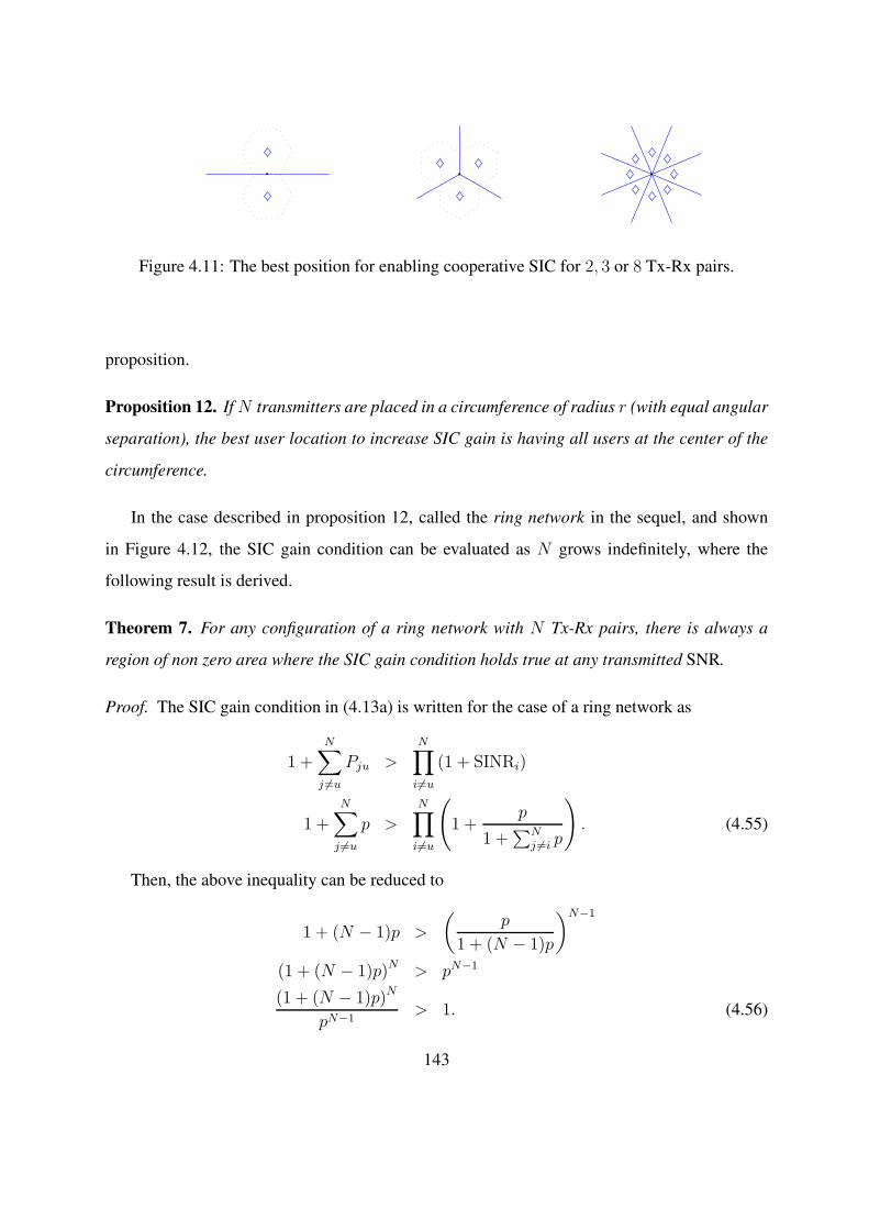
Figure 4.11: The best position for enabling cooperative SIC for 2, 3 or 8 Tx-Rx pairs.

proposition.

Proposition 12. IfN transmitters are placed in a circumference of radius r (with equal angular

separation), the best user location to increase SIC gain is having all users at the center of the

circumference.

In the case described in proposition 12, called the ring network in the sequel, and shown

in Figure 4.12, the SIC gain condition can be evaluated as N grows indefinitely, where the

following result is derived.

Theorem 7. For any configuration of a ring network with N Tx-Rx pairs, there is always a

region of non zero area where the SIC gain condition holds true at any transmitted SNR.

Proof. The SIC gain condition in (4.13a) is written for the case of a ring network as

1 +N∑

j 6=u

Pju >N∏

i 6=u

(1 + SINRi)

1 +

N∑

j 6=u

p >

N∏

i 6=u

(

1 +p

1 +∑N

j 6=i p

)

. (4.55)

Then, the above inequality can be reduced to

1 + (N − 1)p >

(p

1 + (N − 1)p

)N−1

(1 + (N − 1)p)N > pN−1

(1 + (N − 1)p)N

pN−1> 1. (4.56)

143

Finally, it is easily verified that the inequality (4.56) is always true for any value p and any

number of Tx-Rx pairs. For the smallest possible value N = 2, the inequality holds true

(1 + p)2 > p, (4.57)

or for asymptotically large value of N

limN→∞

(1 + (N − 1)p)N

pN−1= ∞ > 1, (4.58)

which proves that a non-empty region exists where SIC gain holds true in a ring network at any

transmitted SNR and any number of Tx-Rx pairs.

Another important feature of a ring network is that if all users are placed in the middle, then

any user could perform SIC and all corners are achievable without degradation. This implies

that the SIC sum rate is

SRSIC =

N∑

i=1

C

(p

1 + (i− 1)p

)

. (4.59)

In order to quantify the advantage of a ring network configuration, we denote the relative SIC

gain as

Grel =SRSIC

SRIaN. (4.60)

To have a simpler expression, the relative gain is tightly bounded as follows.

Lemma 3. The SIC gain obtained from a ring network of N Tx-Rx pairs can be upper-bounded

as

Grel ≤ 1 +log2

([∏N−1

i=2Ni−iNi−N

] [

1 + 2(N−1)pN

])

N log2

(1+Np

1+(N−1)p

) . (4.61)

Proof. See Appendix C.0.4.

In Figure 4.12 the gains due to the use of SIC show the immense potential of ring network

configurations. For large number of Tx-Rx pairs the network capacity can achieve a 2, 5, or up

to 10-fold increase in the high-SNR regime. Ring networks remain an interest benchmark for

hot spots and scenarios where users concentrate on reduced areas.

144

−10 0 10 20 301

2

3

4

5

6

7

8

9

10

min SNR p (dB)

Grel

2 4 6 8 101

2

3

4

5

6

7

8

9

10

# Tx-Rx pairs N

Grel

Upper bound

Grel

N = 10

N = 5

N = 2p = 0 dB

p = 10 dB

p = 30 dB

N Tx...

N Rx

Figure 4.12: Ring network: N transmitters in a circle and N receivers in its center. Gains and

upper bounds.

4.4 Effect of small-scale fading

Since all the analysis has been applied on received SNR values, the SIC gain conditions and

their derived results may also apply for fading channels if the coherence time completely spans

the coding block duration and the link adaptation loop latency provides the necessary conditions

to guarantee the scheduling of cooperative SIC. As the study of the effects of fading and multi-

antenna systems requires a thorough and extensive analysis, this section seeks to point out

preliminary results on the impact of small-scale fading and the use of SIC on multi-antenna

channels.

4.4.1 Fading on SIC gain condition

On the 2x2-IC we consider initially the SISO case to evaluate the ergodic sum rates obtained

with SIC and IaN receivers. Let Pji = Pd−αji |hji|2, where hji accounts for the effective channel

145

gain from small-scale fading.

SRSIC1 = EH

[

C(P1) + min

C

(P21

1 + P1

)

, C

(P2

1 + P12

)]

SRIaN = EH

[

C

(P1

1 + P21

)

, C

(P2

1 + P12

)]

. (4.62)

For notation simplicity EH denotes the expectation over all fading variations. Additionally

Pji = γji|hji|2 is a short-hand notation used to state the SIC gain condition under small-scale

fading in the following theorem.

Theorem 8. The SIC gain condition for Rx1 in the 2x2-IC under a small-scale fading is ex-

pressed in terms of the ergodic achievable rates as

e1/γ21E1

(1

γ21

)

>γ2

γ12 − γ2e−1/γ12E1

(−1

γ12

)

+γ2

γ2 − γ12e1/γ2E1

(1

γ2

)

(4.63)

where E1(x) is the exponential-integral function of the first order.


Equation (4.63) shows the inequality of the SIC gain condition in terms of the expected val-

ues of the Shannon capacity as expressed in equation (4.64), stating that in average, the sum rate

using SIC at Rx1 will be greater than using IaN receivers. But it is difficult to understand what

the effect of small-scale fading is from (4.63). A graphical comparison is useful for understand-

ing. The initial (non-fading) SIC gain condition in (4.3a) is equivalent to C(P21) > C(SINR2)

which can be directly compared to the condition derived in Theorem 8 in order to evaluate

the effect of small-scale fading. Figure 4.13 depicts the relative SIC gains as defined in (4.60)

Grel = SRSIC/SRIaN, with and without small-scale fading. In the presence of small-scale fad-

ing, although the sum rate is reduced with respect to a non-fading channel, the relative gain is

increased. The reason is that the SRIaN is more affected than SRSIC.

146

150 160 170 180 190 200 210 220 230 240 2500

1

2

4

6

8

10

d1 (m)

Grel=

SR

SIC/SR

IaN

Rayleigh fading

Non−fading

d2 = 250 m,Rx2 at celledge.

d2 = 150 m.

Figure 4.13: Relative SIC gains for Rayleigh fading and non-fading channels.

4.4.2 Multi-antenna systems on the SIC gain condition

The SIC gain condition in terms of the ergodic capacity

SRSIC1 > SRIaN

EH [C(P21)] > EH

[

C

(P2

1 + P12

)]

(4.64)

may be further analyzed in MISO and SIMO systems.

• Multiple antennas at the transmitter: The use of multiple antennas at the transmitter will

require an additional feedback mechanism to provide the spatial CSI. If the multiple an-

tennas are used to provide transmission diversity, the desired SNR values (Pi) will enjoy

a power gain (in the order of the number of transmit antennas) while the interference

SNR values (Pij) will remain similar in average as the signal precoding is independent of

the interference channels. This fact goes in contradiction with the SIC gain condition as

stated in (4.64), note that P21 and P12 will in average remain equal, while P2 should in-

crease. Thus, reducing SIC gains. In contrast, if the multiple antennas are used for spatial

multiplexing, additional interference signals will arrive from the same distance. These

147

additional signals may be treated as OCI (impacting SIC gains) or may be considered in

a for SIC by increasing the MAC level as described in section 4.2.5. Since the distance

is the same of the multiple interference signals, the situation becomes similar to the ring

network described in section 4.3.4, which is clearly favorable for the use of cooperative

SIC.

• Multiple antennas at the receiver: Multiple antennas at the receiver can also be used

either for multiplexing or diversity. In the case of diversity, the received power is boosted

proportionally to the number of non correlated copies of the signal that can be effectively

combined determined by the number of properly separated antennas. Both the IaN and

SIC receivers will obtain an increased SINR however, the SIC receiver benefits twice of

this effect in a 2-MAC case (orN times in aN-MAC) whereas the IaN receiver only once.

The difference lies in the number of times a SIC receiver has to decode a signal; N − 1

interference signals and 1 desired signal; taking advantage several times of the diversity

gain. When the multiple antennas at the receiver are used for spatial multiplexing, a

thorough analysis is needed to determine whether SIMO or SIC is better to deal with

interference and ultimately increase the system capacity. This analysis is outside the

scope of this thesis.

4.4.3 Success probability analysis

The event of successfully decoding the desired signal at Rxi is composed by the success in

decoding the interference signal and the success of decoding the desired signal once the inter-

ference has been suppressed [75]. Consider that the link ji takes place over a MISO channel

with ηji antennas. The received SNR, Pji follows a gamma distributionGamma(ηji, γji) where

γji = d−αji is the scale parameter and ηji is the shape parameter.

Theorem 9. If a system operates in the (feasible) external corner of a 2x2 IC, the success

probability for Rxi is

PSICi

succ = e−β/γjiηji−1∑

k=0

k∑

l=0

(k

l

)(β/γji)

k

k!

∂lLPi(β/γji)

∂ (β/γji)le−β/γi

ηi−1∑

k=0

(β/γi)k

k!. (4.65)

148

where L denotes the Laplace transform and β is the outage threshold. Additionally, if the system

operates in the corresponding degraded corner point, the success probability for Rxi is

P∗SICi

succ = e−β/γjηj−1∑

k=0

k∑

l=0

(k

l

)(β/γj)

k

k!

∂lLPij(β/γj)

∂ (β/γj)le−β/γi

ηi−1∑

k=0

(β/γi)k

k!. (4.66)


In the SISO case, the χ2 distributions of the fading random variables lose their degrees

of freedom (scale parameter in the gamma distribution) that appear in MISO case. Hence,

following the derivations in Appendix C.0.6, the expressions (4.65) and (4.66) are reduced to

PSICi

succ = e−β

(

1

γji+ 1

γi

)

β2

γi(γji + γiβ)

P∗SICi

succ = e−β

(

1

γj+ 1

γi

)

β2

γi(γj + γijβ)(4.67)

4.5 Centralized Cell Scheduling under Cooperative SIC

Applying the cooperative SIC scheme in a cellular network with many cells may be challenging

as the number of combinations of cells for which the SIC gain conditions need to be checked can

be prohibitively high. Moreover, a central processor has to know all the received power values

to compute the SIC gain conditions and decide which pairs of BSs and users should perform

SIC. In a network formed by transmitters arranged in a hexagonal grid, a Tx can be paired with

any of its six neighbors if the corresponding SIC gain conditions are verified. Furthermore, a

receiver can be selected by multiple transmitters as the one whose signal should be suppressed.

In this section, we present an algorithm for centralized cell scheduling so as to maximize the

system sum rate. We assume that all the values Pi and Pij are available at the central processor

unit and that the cooperative SIC strategy is only used for at most two cells (i.e. 2-level MACs).

For ease of exposition, the following definitions are used:

Master cell (M): a Tx-Rx pair that imposes a rate to another cell in order to perform SIC and

decode the interfering signals. Slave cell (S): a Tx-Rx pair whose rate is imposed by a master

149

cell. For instance, in a two-cell network operating at an external corner point such that Rx1

performs SIC to decode and suppress the signal from Tx2, the Tx1-Rx1 pair forms the master

cell while the Tx2-Rx2 link is in a slave cell. Consequently, a scheduler that maximizes the sum

rate should be designed under the following premises:

• A master cell cannot be a slave cell simultaneously.

• A master cell has only one slave (only 2-level MACs considered).

• A slave cell may have several masters if the sum rate is increased (cf. equation (4.35)).

Algorithm 1 is used in a network where each cell has already selected one user. This implies

that if there are multiple users on each cell another algorithm should determine which user

should be served.

Once all SIC gain conditions are checked, the scheduler verifies that each slave is linked to

the best master(s) set. Note that if several masters impose a rate constraint on the same slave,

the slave should take the minimum of all rates, which may reduce the SIC gains. Having a

list of slaves paired to the best master(s) S∗list, where the best master(s) are those producing the

largest sum rate, all conflicts should be identified. For each pair (S,M) ∈ S∗list a conflict is

formed by all pairs where the slave S is also a master or the master M is also a slave. Finally,

an exhaustive search over all valid combinations of Master/Slave allocations is done to find the

largest sum rate. Although fairness is not analyzed, it can be pointed out that the SIC gain

conditions activate mainly for celledge users.

4.6 Numerical Results

4.6.1 Two-cell network

The cooperative SIC is tested initially in a two-cell network. The purpose is to understand how

often is the SIC gain condition activated and what is the average value of the SIC gain. To

consider OCI, is important to note that if a user is very close to a celledge, the network will

150

Algorithm 1 Sum rate maximization using SIC in multicell networks

N ⇐ number of cells.

U ⇐ number of users per cell.

1. Check SIC gain conditions for all cells, users and neighbors.

for all n = 1 to N , i = 1 to U , j = 1 to 6 do

if: Pji/(1 + POi) > Pj/(1 + Pij + POj), then [i, j] → SIClist

end for

return SIClist, where L = |SIClist|.

return M ⇐ set of all Masters (M).

return S ⇐ set of all Slaves (S).

2. Find the best Master(s) for each slave.

for i = 1 to L do

find all possible M for Si.

find the subset of M with max Sum Rate.

end for

return S∗list where S = |S∗list|.

3. Find the best M-S allocation without conflicts

for i = 1 to S do

Find all M-S conflicts for (Si,Mi) where:

conflict := (Si,Mi)|Si ∈ M∪Mi ∈ (S ∪M\Mi)

end for

return Conflictslist where C = |Conflictslist|

return V =∏Cj |conflictj | where V is the number of valid M-S combinations.

if V = 0, then S∗list is the M-S allocation A.

for i = 1 to V do

Calculate the system Sum Rate for each feasible allocation

end for

return A, where A ∈ N2×n is the best M-S allocation and n is the number of M-S pairs.

151

−500 0 500−500

0

500hexa−hexa

−500 0 500−500

0

500tri−hexa

−500 0 500−500

0

500tri−tri

Figure 4.14: User distributions in a 2-cell network.

probably decide to apply cooperative SIC between those two cells. Hence, OCI will probably

not include the strongest interferer for a given receiver, but since not all the six cells can be

included on the cooperative scheme, some OCI will be present in a real network. To consider

different levels of OCI, there are three different scenarios where the users will be randomly

placed as shown in Figure 4.14

The SIC success rate is defined as the rate of activation of the SIC gain condition. Figures

4.15, 4.16 and 4.17, show that cooperative SIC gives large gains in the absence of OCI, but

when OCI is included, the SIC success rate and the SIC gain are strongly reduced. The only

gain that preserves a considerable value is seen in the 5% rate, where in the tri-tri case reaches

a 25% increase.

Finally, considering only the case where users are randomly placed in both triangles (see

Figure 4.14), the variation of the gains with respect to the minimum SNR received in the cor-

ner hexagon is shown in Figure 4.18. The encouraging result is that for reasonable values of

received SNR, celledge users (5%-rate) see their average rate increase between 20% and 25%.

This gain is only obtained having cancelled the strongest interferer and includes all other OCI

sources around, showing the great potential of cooperative SIC for N > 2.

152

0 5 10 15 200

0.5

1

Avg Sum Rate b/s/Hz

CDF: hexa−hexa, no OCI, p = 30 dB, r = 250

IaN

SIC

0 5 10 15 200

0.5

1

Avg Sum Rate b/s/Hz

CDF: hexa−hexa + OCI

SIC succ rate = 82%

Sum rate gain = 18%

5% rate gain = 75%

SIC succ rate = 3.4%

Sum rate gain = 0.2%

5% rate gain = 4.2%

Figure 4.15: Sum rate CDF for random users in both hexagons.

0 5 10 15 200

0.5

1

Avg Sum Rate b/s/Hz

CDF: tri−hexa, no OCI

0 5 10 15 200

0.5

1

Avg Sum Rate b/s/Hz

CDF: tri−hexa + OCI

IaN

SIC

SIC succ rate = 96%

Sum rate gain = 40%

5% rate gain = 159%

SIC succ rate = 12%

Sum rate gain = 0.6%

5% rate gain = 16%

Figure 4.16: Sum rate CDF for random users in one hexagon and one triangle.

153

0 5 10 15 200

0.5

1

Avg Sum Rate b/s/Hz

CDF: tri−tri, no OCI

0 5 10 15 200

0.5

1

Avg Sum Rate b/s/Hz

CDF: tri−tri + OCI

IaN

SIC

SIC succ rate = 98%

Sum rate gain = 74%

5% rate gain = 292%

SIC succ rate = 17%

Sum rate gain = 1%

5% rate gain = 24%

Figure 4.17: Sum rate CDF for random users in both triangles.

4.6.2 21-Cell Network

A network of 7 tri-sector BSs forms a 21-cell hexagonal grid as shown in Figure 4.19. Observe

that OCI is present at each cell differently; the outer cells have 2 or 3 neighbors while the inner

cells have 6.

The system parameters are based on LTE simulation scenario known as “3GPP case 1”

described in [81]. Its main values are summarized in table 4.1. CAP is the cell antenna pattern

and the link budget adjustment of −7 dB includes minor factors explained in the cited reference.

In this case, the SIC success rate indicates the average number of cells involved in the

cooperative SIC scheme (either as master or slave) at any given realization. In Figure 4.19, 1/3

of the cells have receivers performing SIC. The system gain is the gain in terms of sum rate

when cooperative SIC is performed as compared to IaN considering all cells, even those not

using SIC. The SIC gain is the gain in sum rate with respect to IaN considering only those cells

154

0 5 10 15 20 25 30 35 400

5

10

15

20

25

30

35

40

45

50

Cell edge power p (dB)

Gain

(%

)

5% Rate gain

Avg Sum rate gain

5% Rate gain OCI

Avg Sum rate gain OCI

Figure 4.18: Sum rate and 5%-rate gains for radom users in both triangles.

involved in the cooperative SIC.

In Figure 4.20, the effect of increasing the transmit power and the number of users is stud-

ied. The left subfigure shows how the SIC success rate increases with the system SNR. This

is explained by the fact that higher transmit power enlarges the SIC gain region. On the right

subfigure the SIC gain averaged over different user locations is compared to the average sys-

tem sum rate. Clearly, when the number of users/cell is increased, the probability of finding

the best pair for SIC gains is increased, yielding in significant system performance gain. How-

ever, the proposed centralized algorithm may become computationally complex and efficient

decentralized scheduling algorithms are required to determine the best user sets to select.

155

Table 4.1: Simulation parameters and values.

Parameter Value

Inter-BS distance (km) 0.5

Min BS-UE distance (km) 0.02

Pathloss (d in km) 148.1 + 37.6 log10(d) dB

Horizontal CAP, θ in () −min(12(θ/70)2, 20) dB

Noise power + Noise figure −174dBm + 9dB

Link budget adj. −7dB.

−800 −400 0 400 800

−800

−400

0

400

800

Master Slave

SIC succ. rate = 33.33%

SRIaN

= 40.75 (b/s/Hz)

SRSIC

= 43.16

System Gain = 5.88%

SIC Gain = 25.45%

Figure 4.19: 21-cell network layout. Users are placed randomly, arrows indicate Master-Slave

relations. The values on the right-hand side are calculated for this particular realization.

156

0 10 20 3015

20

25

30

35

40

45

50

55

60

65

SNR at cell−edge (dB)

SIC

su

cc.

rate

(%

)

0 10 20 30 4010

20

30

40

50

60

70

80

Avg system sum rate gain (%)

Avg

SIC

ga

in (

%)

1 users/cell

2 users/cell

3 users/cell

1 users/cell

2 users/cell

3 users/cell

Figure 4.20: System performance with respect to the number of users per cell.

157

Appendices

159

Appendix C

Appendix C

C.0.3 Proof of proposition 8

Take any internal corner of a polyhedron where SIC gain condition is attained. Without lose

of generality, we use the polyhedron of the capacity region of the MAC at Rxu where 1 +∑N

j 6=u Pju >∏N

i 6=u (1 + SINRi). The internal corner is

[R1u, R2u, . . . Ru] =

[

C (P1u) , C

(P2u

1 + P1u

)

, . . . C

(

Pu

1 +∑N

j 6=u Pju

)]

If the corner is feasible, then

Rju < C (SINRj) , ∀j,

and the sum rate in the corner would be

SRSICu <

N∑

j=1

C (SINRj)

< SRIaN,

which implies that the interior corner feasibility and the SIC gain condition SRSICu < SRIaN

are in contradiction. Then, if the corner is degraded to obtain its feasibility

Rju = C (SINRj) , ∀j

161

and therefore, comparing the sum rates

SRSICu =N∑

j=1

C (SINRj) = SRIaN,

which proves that there is no SIC gain.

C.0.4 Proof of Lemma 3

The relative gain for the ring network can be expressed as

Grel =SRSIC

SRIaN=

∑Ni=1C

(p

1+(i−1)p

)

NC(

p1+(N−1)p

)

=log2

(∏N

i=11+ip

1+(i−1)p

)

log2

(1+Np

1+(N−1)p

) . (C.1)

The argument of the logarithm can be simplified as follows

1+ip1+(i−1)p

1+Np1+(N−1)p

=1 + (N + i− 1)p+ (Ni− i)p2

1 + (N + i− 1)p+ (Ni−N)p2

=1 + (N + i− 1)p+ (Ni−N)p2 − (i−N)p2

1 + (N + i− 1)p+ (Ni−N)p2.

In the case where i = 1

1 + p1+Np

1+(N−1)p

=1 +Np + (N − 1)p2

1 +Np

≤ 1 + limp→∞

(N − 1)p2

1 +Np

≤ 1 + 2(N − 1)

Np. (C.2)

And in the case where i > 1

1 + p1+Np

1+(N−1)p

= 1 +(N − i)p2

1 + (N + i− 1)p+ (Ni−N)p2

limp→∞

(N − i)p2

1 + (N + i− 1)p+ (Ni−N)p2=

N − i

Ni−N. (C.3)

162

After replacing (C.2) and (C.3) and some algebraic manipulation we get

log2

(∏N

i=11+ip

1+(i−1)p

)

N log2

(1+Np

1+(N−1)p

) ≤

log2

([1+Np

1+(N−1)p

]N [∏Ni=2 1 +

N−iNi−N

] [1 + 2N−1

Np])

N log2

(1+Np

1+(N−1)p

)

= 1 +log2

([∏N

i=2 1 +N−iNi−N

] [1 + 2N−1

Np])

N log2

(1+Np

1+(N−1)p

)

= 1 +log2

([∏N−1

i=2Ni−iNi−N

] [1 + 2N−1

Np])

N log2

(1+Np

1+(N−1)p

) .

C.0.5 Proof of Theorem 8

First, the case where C(P21/(1+P1)) > C(P2/(1+P12)) can be discarded since in average the

inequality always holds true. Then C(P21/(1 + P1)) < C(P2/(1 + P12)) is considered. Using

the linearity of the expectation operator, the inequality in (4.3b) yields

SRSIC1 > SRIaN

EH [C(P21)] > EH

[

C

(P2

1 + P12

)]

. (C.4)

Considering Rayleigh fading and SISO channels, any received SNR e.g. Pi = γi|hi|2 follows

an exponential distribution with cdf

FPi(x) = 1− ex/γi . (C.5)

Using the law of total probability

FSINR2(x) = P (SINR2 < x)

= P (h2 < x(1 + h12))

= 1−

[γ2

xγ12 + γ2

]

e−x/γ2 .

Then substituting the ergodic rates with Lemma A.0.1 both expected values are reduced to

EH [C(P21)] =

∫ ∞

0

e−x/γ21

1 + xdx

EH

[

C

(P2

1 + P12

)]

=

∫ ∞

0

γ2e−1/γ2

(1 + x)(γ2 + γ12x)dx.

163

Finally, using the exponential integral definition and a useful integral from [82] as

∫ ∞

x

e−x

xdx = E1(x),

∫ ∞

0

e−ax

(x+ b)(x+ 1)dx = (1− b)−1eabE1(ab) + (b− 1)−1eaE1(a),

the proof is completed.

C.0.6 Proof of Theorem 9

PSICi

succ = PIntsucc × P

Sigsucc

= P

(Pji

1 + Pi> β

)

× P (Pi > β)

(C.6)

Following the same derivations as in Appendix A.0.8, we prove first the success probability

for the interferer term

PIntsucc = e−β/γji

DoFji−1∑

k=0

k∑

l=0

(k

l

)(β/γji)

k

k!

∂lLPi(β/γji)

∂ (β/γji)l,

then the success probability for the signal term

PSigsucc = e−β/γi

DoFi−1∑

k=0

(β/γi)k

k!. (C.7)

For the degraded case, the only variation is to replace the interferer term as

PIntsucc = P

(Pj

1 + Pij> β

)

. (C.8)

164

Part IV

Conclusions and Perspectives

165

Conclusions

Recently, cellular networks have become denser, and need to provide a diversified palette of

communication services, which resulted in both traffic volume and data rate increase. As a re-

sult, increasing the capacity of cellular networks is crucial, and interference mitigation has been

identified as one of the key issues and has attracted significant attention from both industry and

academia. This dissertation provided performance analysis and evaluation of interference miti-

gation techniques for the downlink of future cellular networks, and in particular techniques such

as CoMP at the transmitter side and SIC at the receiver side. Although in theory network coop-

eration has shown promising results, in practice the gains do not seem to materialize and better

cooperation techniques need to be evaluated in realistic scenarios suitable for implementation.


First cooperative techniques at the transmitter side, also known as CoMP, were investigated in

two of the most commonly used transmission modes: CBF and JT. A theoretical framework was

derived (see section 2.2) to precisely measure the impact of different impairments that are often

discarded in previous work in the literature. The quantization error is considered by extending

RVQ analysis. The different delays incurred in the feedback process are included using a Gauss-

Markov process, while unequal path-loss and OCI are accounted by means of moment matching

approximations of gamma distributions. The validity of the derived closed form expressions for

both achievable sum rate and success probability was extensively verified by simulations and

comparisons with LTE parameters. CoMP was proved to be highly sensitive to quantization

and delay errors requiring more advanced feedback techniques for an efficient implementation.

167

To maximize the sum rate of different types of CoMP transmissions, a multi-mode transmis-

sion scheme was proposed (section 2.4) based exclusively on known system parameters. MU-JT

achieves the best ergodic capacity in the high-SNR and high feedback resolution regimes. How-

ever, the rates are only slightly larger than those obtained with CBF without the need for data

sharing and strict synchronization requirements as in JT. Finally, CoMP was also compared

with a non-CoMP transmission (MRT) in section 2.6, to identify the cell regions where CoMP

yields capacity gains. The result shows that CoMP is only beneficial when the users are very

close to the cell-edge and the region can be extended towards the center of the cell by increas-

ing the feedback resolution. Additionally, the need for more efficient feedback mechanisms

was investigated in chapter 3, proposing adaptive feedback allocation techniques for SU-JT and

CBF. Both allocation solutions are based on tight approximations of the ergodic capacity and

the quantization error. However, different from previous solutions on this subject, the optimiza-

tion problem was jointly solved without separating the solution into one for the desired signal

and another for the interference terms, avoiding thus suboptimal results. The proposed schemes

not only perform significantly better than the known ones, but may also increase the network

capacity up to 50% with respect to equal bit allocation at the expense of some extra feedback

bits required to inform the users each time the vector allocation is changed.

Cooperative Successive Interference Cancellation

Opposite from CoMP techniques, SIC takes place at the receiver side. SIC is generally related

to the uplink as is known for many years to be a capacity achieving technique for the MAC,

i.e. multiple sources transmit to the same destination. Similarly, many mobiles may transmit to

the same base station in the same time-frequency resource on a given cell. However, chapter 4

proves that SIC can be very useful in the downlink of wireless networks by means of network

cooperation. A basic two cell network is an instance of an IC and can be decomposed in two

related MACs. Under this perspective, it was shown that there is a condition and a transmission

strategy guaranteeing that the use of a SIC receiver brings gains with respect to IaN receivers

(see section 4.2.1). This condition allows to identify the cell regions where SIC is useful as well

168

as it allows to quantify the gain provided. This new transmission strategy is named cooperative

SIC and is extended for the case of N transmitter and receiver pairs where only one of the

receivers uses its SIC capability to decode and suppress all the N − 1 interference signals.

Additionally, it was shown that in the case of N cells, there are∑N

i

(Ni

)possible SIC gains

conditions in which the cooperative SIC strategy could be applied. The conditions under which

several users can activate the SIC receiver simultaneously are also explored in section 4.2.6.

Bounds for the SIC gains were found for the cellular case, where each user is placed in a

different cell obtaining around 150% in the high-SNR regime. Similar bounds were derived

in the case where both users are placed in the same cell. In that scenario, assuming no OCI,

the sum rate can be smaller but the relative gain of SIC with respect to IaN can achieve a

six-fold increase in the high-SNR regime. Furthermore, a different network layout where all

transmitters are placed in a circle and serve an equal number of receivers located in the center

of the circle is identified as the best possible configuration to increase the SIC gain. For this

layout called ring network, it was shown that there is always a region where the SIC gain

condition holds true for any number of transmitter-receiver pairs (see section 4.3.4). The SIC

gain condition was also evaluated under small-scale fading yielding an increase of the relative

gain (SIC vs IaN, see section 4.4.1). In a more practical perspective, the implementation of

the cooperative SIC strategy in a large network was evaluated in section 4.5. An algorithm

was proposed to find the cooperative SIC clusters that maximize the network sum rate for each

network realization, in order to take the largest possible benefit from the SIC usage. Important

gains are observed specially for cell-edge users. Having only one user per cell, the probability

of employing cooperative SIC is low, and the system gains remain lower than 5%. However,

with only 3 users per cell, the SIC gain condition is easily activated and the system capacity can

be increased up to a 60%. Additional numerical results confirm considerable gains both on the

cell-edge and at the system level.

169

Future work

The theoretic framework derived for CoMP can be readily extended for different subjects that

need to be assessed before the technology is suitable for implementation. For instance, the

Gauss-Markov model can be used to differentiate the different delays that feedback suffers: in

the air interface, in the backhaul and the processing time. In this regard, some transmission

modes will be more likely used for cooperation between the different sectors of the same BS

(known as intra-BS CoMP) or for cooperation between sectors of different BS (inter-BS CoMP).

The adaptive feedback allocation technique proposed for SU-JT cannot be easily extended for

MU-JT. The main difficulty lies in the fact that for the multi-user case, it is not easy to find

an approximation of the SINR such that the optimization problem becomes convex. Therefore,

extending our results to the MU-JT case requires a different approach. Integrating the adaptive

feedback allocation techniques with the analytical expressions obtained for CoMP throughput

can be very useful evaluating how more efficient feedback mechanisms enlarge the regions

where CoMP performs better than non-CoMP transmissions, in particular for technologies such

as Distributed Antenna Systems.

Cooperative SIC is a new strategy for interference mitigation and should be analyzed in

multiple practical settings in wireless networks. The role of power control has to be investi-

gated, while flexible power allocation to the different transmitters may generate the necessary

conditions for cooperative SIC in situations where equal power allocation cannot. Addition-

ally, a meticulous analysis of the performance of SIC for MIMO links is needed. It is crucial

to determine what kind of interference should be counter by means of multiple antennas or

by means of SIC. The impact of imperfect feedback and delay in the cooperation process or

scheduling stages can also reduce the SIC performance. In an information theory perspective,

the cooperative SIC strategy can be compared with different transmission schemes used for the

different regimes of the IC. Finally, the problem of flexible user association combined with si-

multaneous cooperative SIC and scheduling appears to be a highly complex and non convex

optimization problem. Efficient solutions are needed to avoid exhaustive search, allowing for

an easier implementation of a centralized scheduler that takes into account all these variables.

170

Part V

Bibliography

171

Bibliography

[1] ICT facts and figures 2013. International Telecommunications Union, 2013.

[2] D. Tse and P. Viswanath. Fundamentals of wireless communication. Cambridge University

Press, 2005.

[3] T. S. Rappaport. Wireless communications, principles and practice. Prentice Hall, 2002.

[4] A. Goldsmith. Wireless communications. Cambridge University Press, 2005.

[5] Y. Bouguen, E. Hardouin, A. Maloberti, and F.X. Wolff. LTE et les réseaux 4G. EY-

ROLLES, 2012.

[6] A. Lozano and N. Jindal. Transmit diversity vs. spatial multiplexing in modern mimo

systems. IEEE Trans. on Wireless Commun., 9(1):186–197, 2010.

[7] L. R. Kahn. Ratio squarer. Proc. IRE, 42:1704, Nov 1954.

[8] S. M. Alamouti. A simple transmit diversity technique for wireless communications. IEEE

Journal on Sel. Areas in Commun., 16(8):1451 – 1458, October 1998.

[9] E. Telatar. Capacity of multi-antenna Gaussian channels. European Trans. Telecommun.,

6:585–595, 1999.

[10] G.J Foschini and M.J. Gans. On limits of wireless communications in a fading environ-

ment when using multiple antennas. Wireless Pers Commun, 6:311–335, March 1998.

173

[11] V. Tarokh, N. Seshadri, and A. R. Calderbank. Space-time codes for high data rate wireless

communication: Performance criterion and code construction. IEEE Trans. on Inform.

Theory, 44(2):744–765, March 1998.

[12] L. Zheng and D. Tse. Diversity and multiplexing: A fundamental tradeoff in multiple

antenna channels. IEEE Trans. on Inform. Theory, 49(5), May 2003.

[13] J. Zhang, R.W. Heath, M. Kountouris, and J. G. Andrews. Mode switching for the multi-

antenna broadcast channel based on delay and channel quantization. EURASIP Journal

on Adv. Sig. Proc., Sp. Issue on Multiuser Limited Feedback, 2009.

[14] D. Gesbert, S. Hanly, H. Huang, S. Shamai, O. Simeone, and Wei Yu. Multi-cell mimo co-

operative networks: A new look at interference. IEEE Journal on Sel. Areas in Commun.,

28(9):1380–1408, 2010.

[15] J. Jose, A. Ashikhmin, T.L. Marzetta, and S. Vishwanath. Pilot contamination and pre-

coding in multi-cell TDD systems. IEEE Trans. on Wireless Commun., 10(8):2640–2651,

2011.

[16] F. Rusek, D. Persson, B.K. Lau, E.G. Larsson, T.L. Marzetta, O. Edfors, and F. Tufvesson.

Scaling up MIMO: Opportunities and challenges with very large arrays. 30(1):40–60,

2013.

[17] D. López-Pérez, I. Guvenc, G. De la Roche, M. Kountouris, T.Q.S. Quek, and J. Zhang.

Enhanced intercell interference coordination challenges in heterogeneous networks. IEEE

Wireless Communications Magazine, 18(3):22–30, 2011.

[18] J.G. Andrews, H. Claussen, M. Dohler, S. Rangan, and M.C. Reed. Femtocells: Past,

present, and future. IEEE Journal on Sel. Areas in Commun., 30(3):497–508, 2012.

[19] A. Lozano, Andrews J.G., and Heath R.W. On the limitations of cooperation in wireless

networks. Proc., Information Theory and its Applications (ITA), pages 123–130, 2012.

174

[20] V.R. Cadambe and S.A. Jafar. Interference alignment and degrees of freedom of the k

-user interference channel. IEEE Trans. on Inform. Theory, 54(8):3425–3441, 2008.

[21] B. Clerckx, H. Lee, Y.-J. Hong, G. Kim,. Rank recommendation-based coordinated

scheduling for interference mitigation in cellular networks. In Global Telecommunica-

tions Conference (GLOBECOM 2011), 2011 IEEE, pages 1–6, Dec 2011.

[22] H. Dahrouj and Wei Yu. Coordinated beamforming for the multicell multi-antenna wire-

less system. IEEE Trans. on Wireless Commun., 9(5):1748–1759, 2010.

[23] G. J. Foschini and K. Karakayali and R. A. Valenzuela. Coordinating multiple antenna

cellular networks to achieve enormous spectral efficiency. 153(4):548–55, August 2006.

[24] D. Lee, H. Seo, B. Clerckx, E. Hardouin, D. Mazzarese, S. Nagata, and K. Sayana. Coor-

dinated multipoint transmission and reception in lte-advanced: deployment scenarios and

operational challenges. IEEE Commun. Mag., 50(2):148–155, 2012.

[25] B. Clerckx, Y. Kim, H. Lee, J. Cho and J. Lee. Coordinated multi-point transmission in

heterogeneous networks: A distributed antenna system approach. In Circuits and Systems

(MWSCAS), 2011 IEEE 54th International Midwest Symposium on, pages 1–4, Aug 2011.

[26] F. Rashid-Farrokhi, K.J.R. Liu, and L. Tassiulas. Transmit beamforming and power control

for cellular wireless systems. IEEE Journal on Sel. Areas in Commun., 16(8):1437–1450,

1998.

[27] M. Schubert and H. Boche. Solution of the multiuser downlink beamforming problem

with individual SINR constraints. IEEE Trans. on Veh. Technology, 53(1):18–28, 2004.

[28] H. Dahrouj and Wei Yu. Coordinated beamforming for the multi-cell multi-antenna wire-

less system. In Information Sciences and Systems, 2008. CISS 2008. 42nd Annual Con-

ference on, pages 429–434, 2008.

[29] N. Jindal. High SNR analysis of MIMO broadcast channels. In Proc., IEEE Intl. Symp.

on Inform. Theory (ISIT), pages 2310–2314, 2005.

175

[30] O. Somekh, O. Simeone, Y. Bar-Ness, and A.M. Haimovich. CTH11-2: Distributed multi-

cell zero-forcing beamforming in cellular downlink channels. In Proc., IEEE Globecom,

pages 1–6, 2006.

[31] P. Marsch and G. Fettweis. On base station cooperation schemes for downlink network

mimo under a constrained backhaul. In Proc., IEEE Globecom, November 2008.

[32] D.J. Love, V.K.N. Lau, D. Gesbert, B.D. Rao and M. Andrews. An overview of limited

feedback in wireless communication systems. IEEE Journal on Sel. Areas in Commun.,

26(8):1341–1365, October 2008.

[33] N. Jindal. MIMO broadcast channels with finite-rate feedback. IEEE Trans. on Inform.

Theory, 52(11):5045–5060, November 2006.

[34] J. Zhang, M. Kountouris, J.G. Andrews, and R.W. Heath. Multi-mode transmission for

the MIMO broadcast channel with imperfect channel state information. IEEE Trans. on

Commun., 59(3):803–814, March 2011.

[35] M. Kobayashi, N. Jindal and G. Caire. Training and feedback optimization for multiuser

MIMO downlink. IEEE Trans. on Commun., 59(8):800–811, August 2011.

[36] N. Lee, W. Shin, Y.-J. Hong and B. Clerckx,. Two-cell MISO interfering broadcast channel

with limited feedback: Adaptive feedback strategy and multiplexing gains. In Communi-

cations (ICC), 2011 IEEE International Conference on, pages 1–5, June 2011.

[37] F. Boccardi, H. Huang, and A. Alexiou. Network MIMO with reduced backhaul require-

ments by MAC coordination. In 42nd Asilomar Conference on Signals, Systems and Com-

puters, pages 1125–1129, 2008.

[38] P. Marsch and G. Fettweis. Uplink CoMP under a constrained backhaul and imperfect

channel knowledge. IEEE Trans. on Wireless Commun., 10(6):803–814, June 2011.

176

[39] J. Hoydis, M. Kobayashi and M. Debbah. On optimal channel training for uplink network

MIMO systems. In Proc., IEEE Intl. Conf. on Acoustics, Speech, and Sig. Proc. (ICASSP),

pages 3056 – 3059, 2011.

[40] Y. Rui, M. Li, P. Cheng, L. Yinhui, A. Guo. Achievable rates of coordinated multi-point

transmission schemes under imperfect CSI. In Proc., IEEE Intl. Conf. on Communications,

2011.

[41] B. Makki, Jingya Li, T. Eriksson, and T. Svensson. Throughput analysis for multi-point

joint transmission with quantized CSI feedback. In Proc., IEEE Veh. Technology Conf.,

pages 1–5, 2012.

[42] R. Bhagavatula and R. W. Heath Jr. Adaptive limited feedback for sum-rate maximizing

beamforming in cooperative multicell systems. IEEE Trans. on Sig. Process., 59(2):800–

811, February 2011.

[43] J. Zhang and J.G. Andrews. Adaptive spatial intercell interference cancellation in multicell

wireless networks. IEEE Journal on Sel. Areas in Commun., 28(9):1455–1467, December

2010.

[44] N. Seifi, M. Viberg, R.W. Heath, J. Zhang, and M. Coldrey. Multimode transmission in

network MIMO downlink with incomplete CSI. EURASIP Journal on Advances in Signal

Processing, page 4, 2011.

[45] R. Ahlswede. Multi-way communication channels. In IEEE International Symposium on

Information Theory (ISIT), pages 103 – 135, 1971.

[46] H. Liao. A coding theorem for multiple access communications. In IEEE International

Symposium on Information Theory (ISIT), 1972.

[47] S. Verdu. Multiuser Detection. Cambridge University Press, 2008.

[48] A. Carleial. A case where interference does not reduce capacity (corresp.). IEEE Trans.

on Inform. Theory, 21(5):569–570, 1975.

177

[49] T. Han and K. Kobayashi. A new achievable rate region for the interference channel. IEEE

Trans. on Inform. Theory, 27(1):49–60, January 1981.

[50] H. Sato. The capacity of the gaussian channel under strong interference. IEEE Trans. on

Inform. Theory, 27(6):786–788, November 1981.

[51] S. Shamai and B. Zaidel. Enhancing the cellular downlink capacity via co-processing at

the transmitting end. In Proc., IEEE Veh. Technology Conf., pages 1745–1749, May 2001.

[52] H. Weingarten, Y. Steinberg, and S. Shamai (Shitz). The capacity region of the Gaus-

sian multiple-input multiple-output broadcast channel. IEEE Trans. on Inform. Theory,

52(9):3936–3964, September 2006.

[53] P. Marsch and G. Fettweis. A framework for optimizing the uplink performance of dis-

tributed antenna systems under a constrained backhaul. In Proc., IEEE Intl. Conf. on

Communications, pages 975–979, 2007.

[54] P. Marsch and G. Fettweis. Coordinated Multi-Point in Mobile Communications. Cam-

bridge University Press, 2011.

[55] V. Jungnickel, L. Thiele, T. Wirth, T. Haustein, S. Schiffermuller, A. Forck, S. Wahls, S.

Jaeckel, S. Schubert, H. Gabler, C. Juchems, F. Luhn, R. Zavrtak, H. Droste, G. Kadel, W.

Kreher, J. Mueller, W. Stoermer, and G. Wannemacher. Coordinated multipoint trials in

the downlink. In GLOBECOM Workshops (GC Wkshps), 2009 IEEE, pages 1–7, 2009.

[56] Irmer, R. and Droste, H. and Marsch, P. and Grieger, M. and Fettweis, G. and Brueck,

S. and Mayer, H.P. and Thiele, L. and Jungnickel, V. Coordinated multipoint: Concepts

performance and field trial results. IEEE Commun. Mag., 49(2):102–111, February 2011.

[57] E. Biglieri, J. Proakis, and S. Shamai (Shitz). Fading channels: Information-theoretic

and communications aspects. IEEE Trans. on Inform. Theory, 44(6):2619–2692, October

1998.

178

[58] K.K. Mukkavilli, A. Sabharwal, E. Erkip, and B. Aaf. On beamforming with finite rate

feedback in multiple-antenna systems. IEEE Trans. on Inform. Theory, 49(10):2563–79,

October 2003.

[59] C. Au-Yeung and D.J. Love. On the performance of random vector quantization limited

feedback beamforming in a MISO system. IEEE Trans. on Wireless Commun., 6(2):458–

462, February 2007.

[60] P. G. Moschopoulos. The distribution of the sum of independent gamma random variables.

Ann. Inst. Statist. Math. (Part A), 37:541–544, 1985.

[61] S. B. Provost. On sums of independent gamma random variables. Statistics, (20):583–591,

1989.

[62] C. A. Coelho and J. T. Mexia. On the distribution of the product and ratio of independent

generalized gamma-ratio random variables. The Indian Journal of Statistics, 69:221–255,

2007.

[63] D. Jaramillo-Ramírez, M. Kountouris, and E. Hardouin. Coordinated multi-point trans-

mission with quantized and delayed feedback. In Proc., IEEE Globecom, December 2012.

[64] A.M. Hunter, J.G. Andrews, and S. Weber. Transmission capacity of ad hoc networks with

spatial diversity. IEEE Trans. on Wireless Commun., 7(12):5058–5071, 2008.

[65] 3gpp ts 36.211 v10.4.0 (2011-12), physical channels and modulation.

http://www.3gpp.org, December 2011. [Accessed: Jan, 2012].

[66] D. Jaramillo-Ramírez, M. Kountouris, and E. Hardouin. Coordinated multi-point trans-

mission with imperfect channel knowledge and other-cell interference. In Proc., IEEE

PIMRC, September 2012.

[67] H.L Maattanen and K. Schober and O. Tirkkonen and R. Wichman. Precoder partitioning

in closed-loop MIMO systems. IEEE Trans. on Wireless Commun., August 2009.

179

[68] N. Lee and W. Shin. Adaptive feedback scheme on K-cell MISO interfering broadcast

channel with limited feedback. IEEE Trans. on Wireless Commun., 10(2):401–406, Febru-

ary 2011.

[69] R. Bhagavatula and R. W. Heath Jr. Adaptive bit partitioning for multicell intercell interfer-

ence nulling with delayed limited feedback. IEEE Trans. on Commun., 59(8):3824–3836,

August 2011.

[70] S. Yu and H.-B. Kong and Y.-T. Kim and S.-H. Park and I. Lee. Novel feedback bit alloca-

tion methods for multi-cell joint processing systems. IEEE Trans. on Wireless Commun.,

11(9):3030–3036, September 2012.

[71] A. El Gamal and Y.-H. Kim. Network Information Theory. Cambridge University Press,

2012.

[72] F. Baccelli, A. El Gamal and D. Tse. Interference networks with point-to-point codes.

IEEE Trans. on Inform. Theory, 57(5):2582–2596, May 2011.

[73] J. Axnas, Y.-P. Eric Wang, M. Kamuf and N. Andgart. Successive interference cancellation

techniques for LTE downlink. In Proc., IEEE PIMRC, 2011.

[74] Miridakis, N.I. and Vergados D.D. A survey on the successive interference cancellation

performance for single-antenna and multiple-antenna OFDM systems. IEEE Communica-

tions Surveys and Tutorials, 15(1):312–335, 2013.

[75] J. Blomer and N. Jindal. Transmission capacity of wireless ad hoc networks: Successive

interference cancellation vs. joint detection. In Proc. IEEE Int. Conf. on Commun., 2009.

[76] S. Sen and N. Santhapuri and R.R. Choudhury and S. Nelakuditi. Successive interference

cancellation: a back-of-the-envelope perspective. In Proc. ACM SIGCOMM Workshop on

Hot Topics in Networks, 2010.

[77] X. Zhang and M. Haenggi,. The performance of successive interference cancellation in

random wireless networks. In Proc., IEEE Globecom, December 2012.

180

[78] M. Wildemeersch, T.Q.S. Quek, M. Kountouris, A. Rabbachin and C.H. Slump.

Successive interference cancellation in heterogeneous cellular networks. In

http://arxiv.org/abs/1309.6788, Sep 2013.

[79] C. Avin, A. Cohen, Y. Haddad, E. Kantor, Z. Lotker, M. Parter and D. Peleg. SINR

diagrams with interference cancellation. In Proc. 23rd Annual ACM-SIAM Symposium on

Discrete Algorithms, January 2012.

[80] E. Hardouin, M. S. Hassan and A. Saadani. Downlink interference cancellation in LTE:

Potential and challenges. In Proc., IEEE Wireless Networking and Comm. Conf., April

2013.

[81] Further advancements for e-utra physical layer aspects (release 9). 3GPP TS 36.814,

March 2010.

[82] I. S. Gradshteyn and I. M. Ryzhik. Table of Integrals, Series, and Products. Academic,

San Diego, CA, 5 edition„ 1994.

181

Interference mitigation techniques for 4G networks

Documents

Transcript of Interference mitigation techniques for 4G networks