LOSS OF COOLANT ACCIDENT ANALYSIS FOR THE UNIVERSITY...
34
2016 LOSS OF COOLANT ACCIDENT ANALYSIS FOR THE UNIVERSITY OF TEXAS AT AUSTIN TRIGA REACTOR G.KLINE, 2015
Transcript of LOSS OF COOLANT ACCIDENT ANALYSIS FOR THE UNIVERSITY...

2016
LOSS OF COOLANT ACCIDENT ANALYSIS FOR THE UNIVERSITY OF TEXAS AT AUSTIN TRIGA REACTOR G.KLINE, 2015

Table of Contents List of Figures ................................................................................................................................................ 2
List of Tables ................................................................................................................................................. 2
Introduction .................................................................................................................................................. 3
UT TRIGA Characteristics .............................................................................................................................. 3
Decay Heat ................................................................................................................................................ 3
Fuel Element Geometry ............................................................................................................................ 4
Fuel Element Thermodynamic properties ................................................................................................ 4
Basis of Thermodynamic Analysis ................................................................................................................. 5
Stored Energy (𝜌 · 𝑉 · 𝑐𝑝 · 𝑇) ................................................................................................................... 5
Energy Generation (𝑞𝑔𝑒𝑛) ........................................................................................................................ 5
Conduction Heat Transfer (𝑞𝑐𝑜𝑛𝑑) ........................................................................................................... 5
Convection Heat Transfer (qconv) ............................................................................................................... 6
The UT LOCA Model ...................................................................................................................................... 7
Coolant Air Temperature .......................................................................................................................... 7
Finite Element Model Geometry and Basis[12] ...................................................................................... 11
Steady State Finite Element Analysis ...................................................................................................... 12
Transient Finite Element Analysis ........................................................................................................... 15
Model Validation ......................................................................................................................................... 15
Comparison of TRACE and the UT MATLAB model Steady State Temperature Profile .......................... 16
Comparison of FT2 Observations and Calculations (TRACE, UT MATLAB Model) Steady State
Temperature Response to Power Operation .......................................................................................... 17
Comparison of FT2 Observations and Calculations (TRACE, UT MATLAB Model) Transient Temperature
Response to Shutdown from Normal Operations .................................................................................. 17
Summary ................................................................................................................................................. 18
Results and Parametric Variation ............................................................................................................... 18
References .................................................................................................................................................. 21
Code ............................................................................................................................................................ 22
UT LOCA Model ....................................................................................................................................... 22
Channel Air Temperature........................................................................................................................ 30

List of Figures Figure 1. Axial Peaking Factor in Fuel Element ............................................................................................. 4
Figure 2. Channel Air Model Geometry ........................................................................................................ 8
Figure 3. Channel Air Iterative Segment ....................................................................................................... 9
Figure 4. Finite Element Radial Geometry .................................................................................................. 11
Figure 5. Finite Element Energy Balance ..................................................................................................... 13
Figure 6. TRACE and UT LOCA model steady state temperature profiles ................................................... 16
Figure 7. Comparison of Temperatures from Calculations and Observations at Varying Power Levels .... 17
Figure 8. Fuel Temperature, Measuring Channel & Calculations Following Reactor Scram ...................... 18
Figure 9. LOCA Cladding Temperature vs Time .......................................................................................... 19
Figure 10. Region of Acceptable Operations for Fuel Element Specific Power and Air Temperature ....... 19
Figure 11. Peak Fuel Temperature during Loss of Coolant Accident .......................................................... 20
List of Tables Table 1. Conduction and Convection Terms: ..................................................................................... 13
Table 2. Generation and Temperature Independent Terms ............................................................... 14
Table 3.Matrix Elements .................................................................................................................. 14
Table 4. Matrix Formula: .................................................................................................................. 14

Introduction Recent relicensing called for a study of fuel cladding response to a Loss of Coolant Accident (LOCA). Focusing on the maximum cladding temperature achieved.[1], [2] To facilitate this a one-dimensional radial model was created to solve for the peak temperature in the core limited area. The loss of coolant accident (LOCA) analysis assumes steady state reactor operation at equilibrium (limiting core configuration conditions) followed by an instantaneous reactor scram with the water cooling simultaneously replaced with air cooling. The analysis models radial heat transfers from the center of the element outward to the air at the axial location/segment of the hot channel fuel element with the maximum specific axial power. This LOCA analysis includes (1) an overview of the analysis, (2) specific characteristics of UT TRIGA system, (3) the basis of thermodynamic analysis, (4) development of the UT finite element analysis model, (5) validation of the model against independent analytical method and against measured data, and (6) analysis of the thermodynamic characteristics following a LOCA with initial conditions established by the limiting core configuration.
UT TRIGA Characteristics
The University of Texas TRIGA mk. II uses LEU 8.5wt% U with a ZrH ratio of 1.6. The physical properties of the fuel are taken from Simnad[3] while the decay heat transient is taken from University of Kansas[4]. Decay heat is assumed to have the same spatial distribution as power generation during operation. Core limiting configurations were calculated using neutronics analysis.
Decay Heat Calculations with TRACE indicate the maximum power for a fuel element with an acceptable critical heat flux ratio of 2.0 is slightly less than 24kW. Neutronics analysis with the fuel element divided into 15 equal axial segments shows the maximum power generation within a single axial segment is 1.2 times the average segment. The decay power fraction remaining after an abrupt shutdown is found by the equation below:
𝑅(𝑡) =0.04856 + 0.1189 · log10 𝑡 − 0.103 · (log10 𝑡)
2 + 0.000228 · (log10 𝑡)3
1 + 2.5481 · log10 𝑡 − 0.19632 · (log10 𝑡)2 + 0.05417 · (log10 𝑡)
3
(1)
The fuel temperature of the element producing the maximum power level in the core, the “hot channel,” is the most severe condition radially in the core, so its most limiting axial segment is the highest rate of heat production in the core. Thus, this is where the LOCA is analyzed.

For the limiting case, the maximum specific power and the decay power fraction in the fuel element is calculated from the maximum axial peaking factor for the fuel element using:
𝑞𝑔𝑒𝑛,𝑖(𝑡, 𝑟) = 1.2 · 𝑞𝑔𝑒𝑛(𝑟) · 𝑅(𝑡) (2)
The 1.2 is a peaking factor from the SCALE analysis, this also provides the radial flux distribution.
Fuel Element Geometry
The fuel element model in this analysis is a set of concentric cylinders representing a zirconium rod at the center, the fuel matrix, a gas-gap between the fuel and cladding, and cladding. The dimensions are taken from the GA drawings and UT Technical Specifications. The Zirconium fill rod radius is 0.003175m. The fuel matrix outer diameter is 1.47 in (0.018771m) diameter. The gas gap is approximately 0.005 in (1.97E-5 m). Cladding is 0.020 in (0.000508m) thick. The total heated length of the fuel (section with Zr-U fuel matrix) is 15 in, segmented for thermal hydraulic analysis into 15 equal lengths leaving a height of 0.0254m.
Fuel Element Thermodynamic properties
Simnad[3] provides a number of mechanical characteristics and equations for fuel quantities. The thermal conductivity (k) is given, density is calculated from a given equation for a specific Zr:H ratio of 1.6. Density is based off of an equation for the 8.5 wt.% U:
𝜌𝐹𝑢𝑒𝑙 =1
(𝑈𝑤𝑡%𝜌𝑈
) +(1 − 𝑈𝑤𝑡%)
𝜌𝑍𝑟
(3)
Figure 1. Axial Peaking Factor in Fuel Element

Where Utw% is uranium weight per cent, ρU is the density of uranium, and ρU is the density of zirconium. Simnad provides the temperature (T) dependent volumetric heat capacity (cp,vol):
𝑐𝑝,𝑣𝑜𝑙 {𝐽
𝑚3𝐾} = 2.04 + 4.17𝑒 − 3 · 𝑇 (4)
Specific heat capacity (cp,fuel) is calculated as the ratio of eqn. (4) to eqn. (3).
𝑐𝑝,𝑓𝑢𝑒𝑙 {𝐽
𝑘𝑔 ∗ 𝐾} =
𝜌𝐹𝑢𝑒𝑙𝑐𝑝,𝑣𝑜𝑙
(5)
Basis of Thermodynamic Analysis
The steady state and transient analyses can be solved by building a heat balance across a series of finite elements whose energy relation can be built from the following equation[5], [6]:
�̇�𝑠𝑡 = �̇�𝑔𝑒𝑛 + �̇�𝑖𝑛 − �̇�𝑜𝑢𝑡
(6)
Where, �̇�𝑠𝑡 is the stored energy in the structure, �̇�𝑔𝑒𝑛 is energy generated within the structure,
�̇�𝑖𝑛 is energy transferred into the structure, and �̇�𝑜𝑢𝑡 is the energy transferred out of the structure. This model translates physically into:
𝜌 · 𝑉 · 𝑐𝑝 ·𝑑𝑇
𝑑𝑡= 𝑞𝑔𝑒𝑛 + 𝑞𝑐𝑜𝑛𝑑 + 𝑞𝑐𝑜𝑛𝑣 (7)
Stored energy (and the associated temperature change) is a function of material density (ρ), specific heat (cp), volume (V), and the conduction, convection, and generation terms (qgen, qcond,
and qconv respectively).
Stored Energy (𝜌 · 𝑉 · 𝑐𝑝 · 𝑇)
Energy storage is the time dependent material property used in the transient portion of the analysis. It is the dominant factor in peak temperatures as it represents a thermal inertial term[5].
Energy Generation (𝑞𝑔𝑒𝑛)
Energy generation in the core is considered a result of fission effects in the fuel only and is considered axially homogenous within the section and radially distributed.
Conduction Heat Transfer (𝑞𝑐𝑜𝑛𝑑)
Heat transfer through conduction within the radius of the fuel element and cladding is modelled with Fourier’s law of conduction using radial geometry:
𝑞𝑐𝑜𝑛𝑑 = −𝑘 · 𝐴𝑠 ·𝑑𝑇
𝑑𝑟 (8)

Where k is thermal conductivity, As is the surface area through which heat transfer occurs,
and 𝑑𝑇
𝑑𝑟 is the rate of temperature change with respect to radial displacement. As
recommended[7], the gas gap is approximated as thermal conductivity, calculated by the gas gap heat transfer coefficient divided by the thickness of the gap.
Convection Heat Transfer (qconv)
Convection heat transfer is modelled using Newton’s law of cooling[5], [6]:
𝑞𝑐𝑜𝑛𝑣 = ℎ · 𝐴𝑠 · (𝑇𝑠 − 𝑇𝑖𝑛𝑓) (9)
Where the outer surface area is As, the wall temperature is Ts, and the bulk coolant temperature is Tinf, and the heat transfer coefficient is h.
The convection heat transfer coefficient is calculated from dimensionless numbers. For natural convection, the significant dimensionless numbers are the Prandtl (Pr), Grashof (Gr), and modified Rayleigh (Ra) numbers. These values, combined with Nusselt (Nu) correlations, lead to the heat transfer coefficients which are used to find the energy transferred via convection[5], [8].
a. The Prandtl number is a measure of the fluid’s viscous diffusion (v) to kinematic
diffusivity (α) of the fluid:
𝑃𝑟 =𝜈
𝛼 (10)
Where α is the thermal diffusivity of the fluid, defined as:
𝛼 =𝑘
𝑐𝑝 · 𝜌 (6)
(11)
b. The Grashof number is a dominant number in natural circulation. It is dependent on both surface temperature and channel temperature, fluid expansion coefficient, gravity, dynamic viscosity and channel dimensions. The Grashof number is defined as:
𝐺𝑟𝑠 =𝑔 · 𝛽 · (𝑇𝑠 − 𝑇𝑖𝑛𝑓) · 𝑠
3
𝜇2 (12)
Where g is the acceleration due to gravity, β is the thermal expansion coefficient of the coolant, s is the channel width, and μ is the dynamic viscosity of the coolant.
c. The Rayleigh number is a function of buoyancy effects and momentum vs vicious diffusions and calculated as below[8],:

𝑅𝑎𝑠 = 𝐺𝑟𝑠𝑃𝑟 =𝑔𝛽𝜌2(𝑇𝑤𝑎𝑙𝑙 − 𝑇𝑓𝑙𝑢𝑖𝑑)𝑠
3
𝜇2𝑃𝑟
(13)
Where s subscript implies channel width is dimension of interest.
d. The Nusselt number relates the conductive and convective heat transfer effects of
the fluid. The heat transfer is driven by the temperature difference and is found through the Nusselt number. A correlation for natural circulation of air in vertical channels for the Nusselt number is[8]:
𝑁𝑢𝑠 =
{
576
[𝑅𝑎𝑠 (𝑠𝑑𝑦)]2 +
2.87
[𝑅𝑎𝑠 (𝑠𝑑𝑦)]1/2
}
−1/2
(14)
e. The average heat transfer coefficient, ℎ̅, can be found from the average Nusselt number using[5], [9]:
ℎ̅ =𝑁𝑢̅̅ ̅̅ 𝑠·𝑘
𝑠 (15)
The UT LOCA Model
The University of Texas Loss of Coolant model is a combination of finite element analysis (FEA) for steady state, and transient fuel conditions, as well as an air channel analysis sub-section to provide effective estimation of air channel heating. This channel sub-model leads to proper parametric variation analysis by giving a real world upper bounding temperature.
Coolant Air Temperature
Parametric analysis ranges needed to be quantified prior to running. In order to find the limiting values of the channel air temperature, a separate, one dimensional vertical model was created independent of the FEA model and geometry used in finding the fuel temperatures. It utilizes an elemental, vertical, constant temperature surface interfacing with buoyant air. See the figure below for details:

The temperature entering the bottom of the channel surrounding the fuel element is the nominal room air temperature following a loss of coolant, 16°C. This value is based on the observed long term average air temperature for the UT TRIGA Reactor Bay. The rise in temperature is found by segmenting the pin vertically. Each iteration has a specific heat flux relative to the temperature difference between the surface and the air, its specific dimensionless parameters, and a constant surface temperature that is user defined. The limiting conditions set the surface temperature at 1150°C as this was the maximum allowable temperature in the fuel, making it the maximum surface temperature. Also, it gives a built in margin to the true maximum air temperature if the surface was the standard limit of 950°C[10]. The change in air temperature across each segment is a function of the heat generated in the segment and the heat transfer coefficient calculated from local non-dimensional parameters. Heat transfer characteristics in convection depend on intrinsic and extrinsic material properties and fluid temperature, with the heat transfer coefficient calculable though the use of dimensionless numbers. The outlet temperature of one region is the inlet temperature of the next. The channel flow heat up model provided an order of magnitude estimation leading to proper parametric variation.
Figure 2. Channel Air Model Geometry
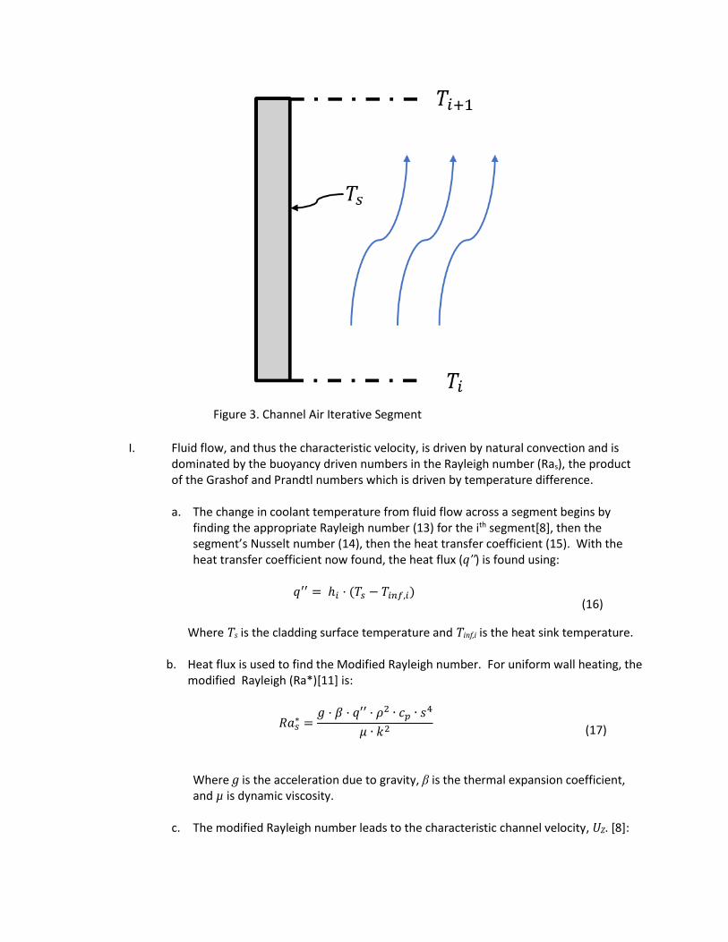
I. Fluid flow, and thus the characteristic velocity, is driven by natural convection and is
dominated by the buoyancy driven numbers in the Rayleigh number (Ras), the product of the Grashof and Prandtl numbers which is driven by temperature difference.
a. The change in coolant temperature from fluid flow across a segment begins by
finding the appropriate Rayleigh number (13) for the ith segment[8], then the segment’s Nusselt number (14), then the heat transfer coefficient (15). With the heat transfer coefficient now found, the heat flux (q’’) is found using:
𝑞′′ = ℎ𝑖 · (𝑇𝑠 − 𝑇𝑖𝑛𝑓,𝑖)
(16)
Where Ts is the cladding surface temperature and Tinf,i is the heat sink temperature.
b. Heat flux is used to find the Modified Rayleigh number. For uniform wall heating, the modified Rayleigh (Ra*)[11] is:
𝑅𝑎𝑠∗ =
𝑔 · 𝛽 · 𝑞′′ · 𝜌2 ∙ 𝑐𝑝 ∙ 𝑠4
𝜇 ∙ 𝑘2
(17)
Where g is the acceleration due to gravity, β is the thermal expansion coefficient, and µ is dynamic viscosity.
c. The modified Rayleigh number leads to the characteristic channel velocity, UZ. [8]:
Figure 3. Channel Air Iterative Segment

(18)
The change in temperature for fluid flow across a segment of the fuel element along the (axial) direction of flow can be calculated with:
19)
d. Where the ΔT is calculated as:
Δ𝑇 =𝑞′′ · 𝐴𝐹𝐸,𝑖
𝜌 · 𝐴𝑓𝑙𝑜𝑤 · 𝑈𝑍 · 𝑐𝑝
(20)
Where UZ is calculated from eqn. (18). This Δ𝑇 is added to the segment’s inlet temperature and becomes the inlet temperature for the next segment. The last segment’s channel temperature represents the culmination of all the heating:
𝑇𝑖𝑛𝑓,𝑖 = 𝑇𝑖𝑛𝑓,𝑖−1 + ∆𝑇𝑖 (21)
II. As an independent calculation to determine limiting values of air temperature, the temperature rise was found through standard gas laws.
a. The characteristic velocity gives a stay time for the air (heated length divided by
characteristic channel velocity). This allows the change in energy to be calculated as follows:
𝑑𝐸 = 𝑞′′ ∙ 𝐴𝑠 ∙ 𝑡𝑠𝑡𝑎𝑦
(22)
Where tstay is the time the cooling air is in contact with the cladding surface.
b. By using the density of air and the volume of the channel, the mass of the air in the space at any given time can be found, by neglecting density changes. Using the equation below, the change in temperature can be found:
𝑞 = 𝑚𝑐𝑣∆𝑇 → (23)
∆𝑇 =𝑞
𝑚𝑐𝑣⟹ 𝑇𝑓 = 𝑇𝑖𝑛𝑖𝑡 + ∆𝑇 (24)
III. Results of calculations for limiting values of the channel air temperature[10]
These two methods routinely agreed across variations in surface temperatures. The geometry in use in reality is far more complex than this simple sub model accounts for, so order of magnitude correlation was acceptable. Especially since the model’s purpose
𝑈𝑧 =𝛼
𝑠√𝑅𝑎𝐿
∗ · 𝑃𝑟
𝑄𝑖̇ = �̇� ∙ 𝑐𝑝 · Δ𝑇 (

was to define reasonable limits for parametric variation. The limiting channel temperature, of 16°C inlet and 950°C surface temperature, is 35.37°C. The bounds selected were based on the 12.5kW fuel element reaching the limiting surface temperature.
Finite Element Model Geometry and Basis[12] The calculation of temperature distribution in the fuel element is accomplished by using the principles of finite element analysis. The fuel element geometry is based on a cylindrical segment. The axial height of the segment is the total heated length (0.381 m) divided by the number of axial segments (15 in this model). Radial dimensions are taken from General Atomics drawings, as specified earlier.
Figure 4. Finite Element Radial Geometry
The FEA radii distribution used in computation was selected based on both parameter validation and computational power available. It was essential to adequately capture the temperature effects in the smaller outer geometries and transitions. Thus the, dr, value near the outer portion is smaller than in the center fuel meat area. This saved on the size of the solution array, but still allows necessary detail. This is a similar method of grid distribution used in higher end CFD programs.

The limiting geometric parameter of concern is the Biot number[5], which relates convective and conductive aspects of the element to its volume to surface area ratio. It is determined using the equation below:
𝐵𝑖 = ℎ·𝐿𝑐
𝑘 (25)
Where, the characteristic length, Lc, is defined as the volume to surface area ratio:
𝐿𝑐 =𝑉
𝐴 (26)
Differential radii in the outer portions of the model were chosen to most accurately subdivide the real geometry of the cladding and the gas gap. Internal fuel differential radii were chosen to minimize the Biot number. In addition to the Biot number, the Fourier number is a transient figure of merit related to the time response and geometry:[5]
𝐹𝑜 =𝛼 · 𝑡
𝐿𝑐 (27)
According to Bergman[5], the Biot number must remain below 0.1, and the Fourier number must remain below 0.5 for 1D lumped parameter FEA to be valid. This was the merit to which the differential radii are chosen.
Steady State Finite Element Analysis
To create a valid transient condition, a valid steady state initial condition must be found, first. To facilitate this, each element is assessed using an energy balance equation across the element. Since the steady state model is not time dependent, the energy balance is reduced to:
(28)
In this analysis, all energy flow is considered into the element. Figure 5 illustrates an element energy balance and temperature definition relationship.
�̇�𝑖𝑛 + �̇�𝑔𝑒𝑛 = �̇�𝑜𝑢𝑡; �̇�𝑜𝑢𝑡 = 0 ⟹ �̇�𝑖𝑛 + �̇�𝑔𝑒𝑛 = 0

Figure 5. Finite Element Energy Balance
A matrix form of this energy balance is developed to solve for the temperature profile.
𝐴�⃑� = �⃑⃑� (29)
Where, �⃑� is a vector representing the radial temperature profile, and �⃑⃑� is a vector representing the energy generation and non-temperature dependent terms. Below is the development of the steady state finite element equations. The cladding end element is the only element containing a convection term, while fuel elements are the only ones containing generation terms. The following relationships are incorporated in the elements of the matrix equations[12]
Table 1. Conduction and Convection Terms:
𝑞𝑔𝑒𝑛,𝑆𝑆,𝑟 = 𝑞𝑚𝑎𝑥 ∙ 𝑞(𝑟) · 𝜋 · 𝑑𝑦 · (𝑟2𝑖2 − 𝑟2𝑖−2
2) (30)
𝑞𝑐𝑜𝑛𝑣,𝑆𝑆 = ℎ𝑤𝑎𝑡𝑒𝑟 · 𝜋 · 𝑟𝑚𝑎𝑥 · 𝑑𝑦 · (𝑇𝑠 − 𝑇𝑖𝑛𝑓) (31)
𝑞𝑐𝑜𝑛𝑑,𝑆𝑆 =2 · 𝜋 · 𝑑𝑦 · 𝑘𝑓𝑢𝑒𝑙 · (𝑇𝑖±1 − 𝑇𝑖)
ln (𝑟𝑙𝑎𝑟𝑔𝑒𝑟𝑟𝑠𝑚𝑎𝑙𝑙𝑒𝑟
) (32)

Table 2. Generation and Temperature Independent Terms
𝑏𝑖 = −𝑞𝑚𝑎𝑥 · 𝜋 · 𝑑𝑦 · (𝑟2𝑖2 − 𝑟2𝑖−2
2); (33)
𝑏𝑒𝑛𝑑−1,4 = 0; (𝑁𝑜 ℎ𝑒𝑎𝑡 𝑔𝑒𝑛𝑒𝑟𝑎𝑡𝑖𝑜𝑛 𝑖𝑛 𝑐𝑙𝑎𝑑𝑑𝑖𝑛𝑔 𝑔𝑎𝑠⁄ ) (34)
𝑏𝑒𝑛𝑑 = −ℎ𝑤𝑎𝑡𝑒𝑟 · 𝜋 · 𝑟𝑒𝑛𝑑 · 𝑑𝑦 · 𝑇𝑖𝑛𝑓 (35)
Table 3. Matrix Elements
𝑨 =
[ 𝒂𝟏𝒂𝟐⋮𝒂𝒋𝒂𝒆𝒏𝒅]
(36)
𝒂𝟏 = [ 𝟐 · 𝝅 · 𝒅𝒚 · 𝒌𝒇𝒖𝒆𝒍 · (𝑻𝒊−𝟏 − 𝑻𝒊)
𝐥𝐧 (𝒓𝟐𝒓𝟏)
,−𝟐 · 𝝅 · 𝒅𝒚 · 𝒌𝒇𝒖𝒆𝒍 · (𝑻𝒊+𝟏 − 𝑻𝒊)
𝐥𝐧 (𝒓𝟐𝒓𝟏)
… ]
(37)
𝒂𝒊
= [… ,𝟐 · 𝝅 · 𝒅𝒚 · 𝒌𝒇𝒖𝒆𝒍(𝒈𝒂𝒔,𝒄𝒍𝒂𝒅) · (𝑻𝒊−𝟏 − 𝑻𝒊)
𝐥𝐧 (𝒓𝟐𝒊−𝟏𝒓𝟐𝒊−𝟑
), −(
𝟐 · 𝝅 · 𝒅𝒚 · 𝒌𝒇𝒖𝒆𝒍(𝒈𝒂𝒔,𝒄𝒍𝒂𝒅)·(𝑻𝒊−𝟏 − 𝑻𝒊)
𝐥𝐧 (𝒓𝟐𝒊−𝟏𝒓𝟐𝒊−𝟑
)
+𝟐 · 𝝅 · 𝒅𝒚 · 𝒌𝒇𝒖𝒆𝒍(𝒈𝒂𝒔,𝒄𝒍𝒂𝒅) · (𝑻𝒊+𝟏 − 𝑻𝒊)
𝐥𝐧 (𝒓𝟐𝒊+𝟏𝒓𝟐𝒊−𝟏
)) ,𝟐 · 𝝅 · 𝒅𝒚 · 𝒌𝒇𝒖𝒆𝒍(𝒈𝒂𝒔,𝒄𝒍𝒂𝒅) · (𝑻𝒊+𝟏 − 𝑻𝒊)
𝐥𝐧 (𝒓𝟐𝒊+𝟏𝒓𝟐𝒊−𝟏
) … ]
(38)
𝒂𝒆𝒏𝒅 = [… ,𝟐 · 𝝅 · 𝒅𝒚 · 𝒌𝒄𝒍𝒂𝒅 · (𝑻𝒆𝒏𝒅−𝟏 − 𝑻𝒆𝒏𝒅)
𝐥𝐧 (𝒓𝒆𝒏𝒅𝒓𝒆𝒏𝒅−𝟏
),
−(𝟐 · 𝝅 · 𝒅𝒚 · 𝒌𝒄𝒍𝒂𝒅 · (𝑻𝒆𝒏𝒅−𝟏 − 𝑻𝒆𝒏𝒅)
𝐥𝐧 (𝒓𝒆𝒏𝒅𝒓𝒆𝒏𝒅−𝟏
)+ 𝒉𝒘𝒂𝒕𝒆𝒓 · 𝝅 · 𝒓𝒆𝒏𝒅 · 𝒅𝒚) ]
(39)
Table 4. Matrix Formula:
�⃑⃑� = 𝑨−1 · �⃑⃑⃑� (40)

The energy generation term in the element is a function of both its axial and radial position. The highest axial peaking factor (1.2) was used to represent the axial cylindrical segment generating the most power. The radial peaking factor, q(r), is found through a curve fit to neutronics code output:
𝑞(𝑟) = ∁𝑎𝑥𝑖𝑎𝑙,𝑝𝑒𝑎𝑘𝑞𝑚𝑎𝑥(247192𝑟3 − 5377𝑟2 + 45.882𝑟 + .7335)
(41)
MATLAB was utilized to build and solve the equation set using native commands that maximize the efficiency and accuracy of the matrix inversion method.
Transient Finite Element Analysis The transient portion of the model takes the initial steady state temperature profile and systematically walks it forward with time, explicitly. The basic concept of an energy balance is again used, with the time dependent components now considered in addition to the other terms. In the UT LOCA model the loss of coolant accident is considered to be instantaneous, and thus the cooling properties switch from water to air at the first iteration.
�̇�𝑠𝑡 = �̇�𝑖𝑛 − �̇�𝑜𝑢𝑡 + �̇�𝑔𝑒𝑛; �̇�𝑜𝑢𝑡 = 0 → (42)
𝜌𝑉𝑐𝑝𝑑𝑇
𝑑𝑡= 𝑞𝑐𝑜𝑛𝑑 + 𝑞𝑐𝑜𝑛𝑣 + 𝑞𝑔𝑒𝑛 → (43)
𝜌𝑉𝑐𝑝(𝑇𝑖
𝑝+1− 𝑇𝑖
𝑝)
∆𝑡= 𝑞𝑐𝑜𝑛𝑑 + 𝑞𝑐𝑜𝑛𝑣 + 𝑞𝑔𝑒𝑛 (44)
This leads to the transient analysis equation set which is related to the steady state equations as follows:
𝑇𝑖𝑝+1
=∆𝑡
𝜌𝑉𝑐𝑝[𝑎𝑖] + 𝑇𝑖
𝑝 (45)
The differential time element is selected based on the Fourier number previously mentioned. Additionally, the code calculates a number of output values including a two-dimensional matrix
�⃑⃑� whose horizontal dimension represents the radial temperature distribution and whose vertical axis represents time. This allows three essential model parameters to be extracted. First, the cladding surface temperature versus time is extracted and used to find peak cladding temperature. Second, the temperature profile across the pin at ti can be found. Third, the maximum temperature both radially and through time can be found[12].
Model Validation After completion of the model building, a series of validation parameters and tests were run.
The first of these was to ensure the steady state temperature profiles between the UT code and the TRACE code matched. Next was to ensure the temperature profiles of a known operating conditions were properly simulated. Third, a sub model was developed using water properties

and the same decay curve. A real reactor scram was recorded using in-house ICS recording[13] whose results were then compared to the model output. Thus, SS and transient portions were tested.
Comparison of TRACE and the UT MATLAB model Steady State Temperature Profile The core configuration contains 114 fuel elements, with a core radial peaking factor
derived from SCALE physics calculation for the core (prior to January 2016) of 1.6, and a maximum axial peaking factor of 1.2. The current normal operating power is 950 kW. The power generated in the maximum segment of the hot channel for comparison using data prior to January 2016 is therefore 12.5 kW.
The steady state solution using water coolant was developed for the maximum power level in a fuel element operating at 12.5 kW and compared to the TRACE calculations Figure 6. The TRACE and FEA calculations are in substantial agreement with experimental data as shown in the figure below:
Figure 6. TRACE and UT LOCA model steady state temperature profiles

Comparison of FT2 Observations and Calculations (TRACE, UT MATLAB Model) Steady State Temperature Response to Power Operation
The MATLAB finite element analysis was applied at power generation in an element from 200 W to the 12.5 kW, and the maximum element temperature compared to the TRACE and FT2 measurements (taken prior to January 2016) across the range.
The TRACE and the MATLAB based steady state temperature calculations in radial locations associated with thermocouples are essential the same. The error is considered acceptable, as the UT model does not consider the effects of nucleate boiling and varying velocity profiles, as Figure 7 below shows.
Figure 7. Comparison of Temperatures from Calculations and Observations at Varying Power Levels
Comparison of FT2 Observations and Calculations (TRACE, UT MATLAB Model) Transient Temperature Response to Shut down from Normal Operations
Transient fuel temperature was observed following a shutdown from power operations at 950 kW (FT2 Data). Calculations were performed to simulate the transient using TRACE (TRACE Calc.) and MATLAB based model (UT MATLAB).

Figure 8. Fuel Temperature, Measuring Channel & Calculations Following Reactor Scram
Summary
Comparison of fuel temperature measured channel data to calculated fuel temperatures during steady state and transient conditions is in good agreement. The agreement between observations and calculations during steady state operations suggests the method is fundamentally correct. The agreement between observations and calculations during transient operations suggests the method will provide reasonably accurate time-dependent calculations.
Results and Parametric Variation
The UT MATLAB model calculation was performed for various values of both air channel temperature and fuel element specific power. The cladding temperature of the fuel element segment generating the highest power in the core is provided in Figure 9 following a shutdown from a limiting operation of 23kW in the element with air cooling at inlet air temperature equal to UT rector bay nominal temperature of 16°C.

Figure 9. LOCA Cladding Temperature vs Time
Fuel element power level and inlet air temperature were varied to provide an indication to sensitivity to the parameters. Air inlet varied from 16°C to 600°C, while fuel element power varied from 12.5kW per pin to 27kW per pin. This ensured all operational areas were covered, and sufficient data existed to curve fit. Figure 11 shows the region of interest in this output.
Figure 10. Region of Acceptable Operations for Fuel Element Specific Power and Air Temperature

Figure 11. Peak Fuel Temperature during Loss of Coolant Accident
For reactor bay air at 16°C, the maximum fuel element power prior to LOCA initiation that could achieve less than 950°C fuel cladding temperature with air cooling is 23.6 kW. At 23 kW generated in the fuel element during operation prior to the LOCA initiation (the maximum power generated in a fuel element in the limiting core configuration), air inlet temperature inlet less than 35°C is calculated not to exceed 950°C fuel cladding temperature. Therefore, a LOCA following normal steady operation with a fuel element operating at 23 kW will not exceed the fuel temperature safety limit. For nominal UT operations of 12.5kW, an air inlet temperature of up to 402°C can exist at the beginning of the casualty to still remain below the 950°C cladding temperature
The UT LOCA model takes place at the point of highest axial power production and only transmits energy radially. In reality the axial conduction effects would work to reduce the overall temperature profile internally, and the additional surface area would help the convective terms. This can be inferred from the lower power production and the high thermal conductivity of the fuel meat. Given the one-dimensional nature of the UT LOCA model, the results for maximum fuel element analysis can be considered conservative. In reality, axial power distribution will result in heat conduction that reduces the peak temperature; since axial conduction is not considered in this analysis and calculated temperatures will be therefore be conservatively higher compared to actual temperatures.

References [1] G. Atomics, “Technical Foundation of TRIGA,” San Diego, CA, 1958. [2] Argonne National Laboratory, “Fundamental Approach to TRIGA Steady-State Thermal-Hydraulic
CHF Analysis,” San Diego, CA, 2007. [3] M. T. Simnad, “The U-ZrHx Alloy: Its Properties and Use in TRIGA Fuel,” Nucl. Eng. Des., vol. 64,
pp. 403–422, 1981. [4] Kansas State, “Kansas State University Safety and Analysis Report ’06.” KSU, Manhatten, 2006. [5] T. L. Bergman, A. S. Lavine, F. P. Incropera, and D. P. DeWitt, Fundamentals of Heat and Mass
Transfer. 2011. [6] F. P. Incropera, D. P. DeWitt, T. L. Bergman, and A. S. Lavine, Fundamentals of Heat and Mass
Transfer, vol. 6th. 2007. [7] Henri Fenech, Heat Transfer and Fluid Flow in Nuclear Systems. Pergamon Press, 1981. [8] M. J. Deborah Kaminski, An introduction to Thermal and Fluids Engineering. Wiley, 2011. [9] C. O. Popiel and J. Wojtkowiak, “Simple formulas for thermophysical properties of liquid water
for heat transfer calculations (from 0 to 150 degrees C) (vol 19, pg 87, 1998),” Heat Transf. Eng., vol. 19, no. 3, pp. 87–101, 1998.
[10] G. Kline, “channel_air_temp_3_0.” Greg Kline, Austin, p. 5, 2015. [11] K. Vafai, C. P. Desai, S. V. Iyer, and M. P. Dyko, “Buoyancy Induced Convection in a Narrow Open-
Ended Annulus,” J. Heat Transfer, vol. 119, p. 483, 1997. [12] G. Kline, “LOCA_8_5_3_FEM.” Greg Kline, Austin, p. 20, 2015. [13] G. Kline, “PXIe_ICS_Power_Cal_Etc_2015.” Greg Kline, Austin, TX, p. 100, 2015.

Code
UT LOCA Model %% HEADER
% UT LOCA
% Author: Greg Kline % Date: 1/21/2015
% Revision 8.5.2
% % Revision Changes:
% - begin mapping a 1D transient, radial, air cooled naturally circulated
% fuel pin immediately after shut down with decreasing decay heat % - 6.0 has liner transient development.
% - 6.1 has radial
% - 6.2 added variable heat transfer coefficient % - 6.3 added variable specific heat capacity and improved check feature
% - 6.4 worked on adjusted dt and shorter t vector
% - 6.5 added function for channel heat calculation % Revision 7
% - 7.0 added radial flux distribution
% - 7.1 added titles to graphs that change % Revision 8
% - 8.0 changed the physical properties of the pin to reflect both the 304SS
% cladding and the gas gap possibly existent in the pin % - 8.1 Working to match TRACE
% - 8.2 Cleaned up code and changed n to meet actual cladding thickness and
% and reduce the gap width to values more realistic % - 8.3 Updating transient solution to fix it for multiple materials
% - 8.4 Updated the length vector to reduce points between the fuel segments
% - 8.4.1 Changed gas from cp to cv. Since the gas gap volume is considered % constant throughout the process
% - 8.4.2 Fixed parenthesis bug
% - 8.5 Made it a function % - 8.5.1 add natural circulation channel Nusselt number relationship
% - 8.5.2 adjusted for a 30C initial water temperature
% - 8.5.3 Added channel air temperature function to the file for the FEM %
%
% function [ mT, t_max ] = LOCA_8_5_3_FEM( qtp, Tia) %
% qtp - Power in the fuel element (W)
% Tia - Air temperature at time of LOCA (C) % mT - Maximum cladding surface temperature (C)
% t_max - Time at which the maximum temperature occurs (s)
% % FEM Pseudo Code
% - Constants
% - Fuel Constants from Simnad, etc. % - Fuel geometry
% - Model Constants
% - Air and water material properties % - Model time parameters
% - Differential time steps % - Time splits
% - Build time vector
% - Build decay heat fraction % - Find specific power
% - Heat transfer coefficients
% - FEA building % - number of points (n)
% - build radial spacing
% - find the radially fractioned specific energy generation % - Find the initial Biot and Fourier values
% - Steady State Initial Condition
% - RHS % - Values of generation and temperature independent terms
% - LHS
% - Matrix of temperature interactions representing temperature

% dependent values of energy equation
% - Build the inner point % - cladding points
% - Gas/fuel interface
% - inner fuel points % - TRACE vector
% - Solve for the temperature profile in steady state
% - Transient problem % - pre-allocate memory
% - Transient loop
% - find the dt for current time space % - find the current dimensionless numbers for channel conditions
% - find the current heat transfer coefficient
% - find the current temperatures in the profile % - find the current model validation values
% - check to see if it is the maximum so far
% - Outputs % - Build a reduced point matrix to save memory
% - Find the maximum temperatures
% - Build output graphs %
% function [ Tinf ] = channel_air_temp_3_0(T_s, Tinit)
% % T_s - Surface temperature (C)
% Tinit - Initial temperature of the inlet channel air (C)
% Tinf - Channel outlet temperature (C) %
% Channel Air Pseudo Code % - Geometry of fuel element
% - Geometry of air channel
% - Iterate up the pin vertically % - Due back of envelope calculations
% - Outputs
function [ mT, t_max ] = LOCA_8_5_3_FEM( qtp, Tia)
tic
display('Initializing LOCA... ');
%% CONSTANTS
% FUEL CONSTANTS % Initial Temp for model VnV
T_init = 30;
% fuel initial pin power (W)
q_total_pin = qtp;
% Axial Peaking Factor
axial_peaking = 1.2435;
%% FUEL CONSTANTS
% pin height (m)
pin_height = .381;
% Pin radius (m)
radius_pin = 0.018771; % .735in inner_radius = 0.003175; %.125in
% clad width (m)
dl_clad = 0.000508;
% vertical sections (#) vertical_sections = 15;
% enrichment percentage (fraction) [UT SAR] Rich = .197; % 19.7%
% density (kg/m^3) [Simnad]

density_U = 19070;
% density of ZrH based on ratio (kg/m^3)[Simnad]
density_Zr = 1 / (.1541 + .0145 * 1.6) * 1000;
% Thermal conductivity fuel [Simnad]
% ( cal / s cm C )
k_fuel_cal = .042;
% ( W / m*K )
k_fuel = 17.5730; % [Simnad]
% Avogadro’s number (atoms/mol)
N_A = 6.022e23;
% Molar mass (g/mol) [Burns]
M_U = 238.07;
% weight percent of Uranium in Triga fuel [UT SAR]
U_wt = .085; % 8.5%
% Material Densities (kg/m^3)
density_fuel = 1 / ( U_wt / density_U + (1 - U_wt) / density_Zr ); %[Simnad] density_gas = .08375; % PNNL
density_304SS = 7740; % makeitfrom.com
% volumetric heat capacity from Simnad (J/ m3 K)
cp_fuel_vol = (2.04 + 4.17e-3 * T_init ) * 1e6;
% Convert to specific heat ( J / kg K )
cp_fuel = cp_fuel_vol / density_fuel; cp_304SS = 500;
cp_gas = 14.53e3; % PNNL ->
cv_gas = 10.16e3; % Hydrogen
% thermal diffusivity ( m^2 / s)
alpha_fuel = k_fuel / ( cp_fuel * density_fuel);
% pin volume (m^3)
vol_pin = pi * pin_height * ((radius_pin-dl_clad)^2 - inner_radius^2);
% specific pin power (W/m^3)
q_dot_max = q_total_pin / vol_pin;
% This is a slice of a potential 2D model of the pin (m)
dy = pin_height / vertical_sections;
%% MODEL CONSTANTS
% Temperatures (C) % find the value using sub-model function
T_inf_air = 1.5 * channel_air_temp_3_0(1150, 16);
% option to set air
% T_inf_air = 20; %Tia;
% Water temperature to build initial condition profile (C)
T_inf_water = 48;
% display temperatures
display(sprintf('T_inf_air is %3.2f C', T_inf_air ));
% Thermal Conductivities (W/mK)
k_air = 0.0257; % engineering toolbox
k_304SS = 16.2; % makeitfrom.com
% Prandtl Number (Pr)
Pr_air = .713; Pr_water = 1.76;
% Kinetic Viscosity (m^2/s)

kinetic_viscosity_air = 15.11e-6;
kinetic_viscosity_water = .279e-6;
% Expansion Coefficient (1/K)
B_air = 3.43e-3; B_water = .207e-3;
% Gradient Prandtl (gPr) gPr_air = (.75 * Pr_air)^.5 / (.609 + 1.221 * Pr_air^.5 + 1.238 * Pr_air)^.25;
gPr_water = (.75 * Pr_water)^.5 / (.609 + 1.221 * Pr_water^.5 + 1.238 * Pr_water)^.25;
% Gravity (m/s^2)
gravity = 9.8066;
%% MODEL TIME PARAMETERS
display(sprintf('Pin power at time 0- is %5.2f W', q_total_pin));
% TIME VECTOR
% Time (s)
dt1 = .00025; dt2 = .0013;
dt3 = .0015;
% Time to split the dt (s)
t_split1 = 1000;
t_split2 = 2000;
% Time vector for LOCA build (s) t = [0:dt1:t_split1 t_split1+dt2:dt2:t_split2 t_split2+dt3:dt3:17000];
% Time for decay heat (log(s)) log_t = log10(t);
% Decay power and radial peaking % Decay Power fraction with time (dimensionless)
Decay_power_fraction = (.04856 + .1189 .* log_t - .0103 .* log_t.^2 + .000228 .* log_t.^3 )./ ...
(1 + 2.5481 .* log_t - .19632 .* log_t.^2 + .05417 .* log_t.^3);
% Decay power with time ( W )
Decay_power_t = (Decay_power_fraction * q_total_pin)';
% Specific energy generation ( W/m^3 )
q_dot = axial_peaking * Decay_power_t / vol_pin; % 1.2 peaking factor
%% HEAT TRANSFER COEFFICIENTS
% Water heat transfer, found using TRACE analysis
h_water = 3200;
% Gas heat transfer from KSU SAR [Whaley] h_gas = 2.84e3;
%% FEA BUILDING % Finite element building
% number of x units to provide adequate spacing for clad and gas geometry(#)
n = 120;
% radius points for determining temperatures (m)
x1 = linspace(inner_radius,radius_pin,n);
% find dx for determination of indices to be used for different materials (m)
dx = x1(2) - x1(1);
% In order to capture clad and gas geometry but not over burden memory usage
% radial spacing near edges is smaller than the spacing in the fuel meat % Fuel meat spaces (m)
xpt1 = linspace(inner_radius,radius_pin-6*dx,19);
% Cladding gas spacing (m)
xpt2 = linspace(radius_pin-5*dx,radius_pin,5);

% build the vector (m)
x = [ xpt1 xpt2 ];
% clad points (#)
% find the number of x points to accurately represent the clad space (#) pts_clad = ceil ( dl_clad / dx );
% gas points (#) % set number of points gas gap occupies (#)
pts_gas = 1; % [Fenech]
% radius vector for determining the volumes for energy generation. Indexing
% requires the volume around a temperature to be half way between the temperatures
% Fuel radial volume points (m) rpt1 = linspace(inner_radius,radius_pin-6*dx,2*19-1);
% clad radial points (m) rpt2 = linspace(radius_pin-5*dx,radius_pin,2 * 5 -1 );
% Build the radial vector m) r_vol = [ rpt1 radius_pin-5.5*dx rpt2 ];
% Set the radial fraction varied energy production (W/m^3) q_r = axial_peaking * q_dot_max * (247192.*xpt1.^3 - 5377.*xpt1.^2 + 45.882.*xpt1 + .7335); % initial condition
q_r_t = (247192.*xpt1.^3 - 5377.*xpt1.^2 + 45.882.*xpt1 + .7335); % radial percentage
% Gas thermal conductivity (W/m K)
k_gas = h_gas * dx;
% For transient problems, validity is reached only if:
% Biot # < .1 % Fourier number < .5(1D) .25 (2D) [Bergman]
L_c_1 = (pi*(r_vol(2)^2 - r_vol(1)^2)*dy) / (dy * 2 * pi * (r_vol(2) + r_vol(1)));
L_c_2 = (pi*(r_vol(end)^2 - r_vol(end-1)^2)*dy) / (dy * 2 * pi * (r_vol(end) + r_vol(end-1)));
Bi_1 = h_water * L_c_1 / k_fuel;
Bi_2 = h_water * L_c_2 / k_fuel;
Fo_1 = alpha_fuel * dt1 / L_c_1^2;
Fo_2 = alpha_fuel * dt1 / L_c_2^2;
check = Fo_1 * (1+Bi_1); % this must remain <= 1/2
%% STEADY STATE INITIAL CONDITION
% set up the FEA
% At = b => t = A-1b
display('Building initial condition');
% Right Hand Side (RHS) % The right hand side of the equation represents the energy generation and
% non-temperature dependent values of the energy balance
% pre-allocate vector b = zeros(length(x),1);
% Most internal fuel point b(1) = -q_r(1) * pi * dy * (r_vol(2)^2 - r_vol(1)^2);
% Boundary with the fluid b(end) = - h_water * pi * 2 * r_vol(end) * dy * T_inf_water; % OLD -q_r(end) * pi/6 * dy * (r_vol(end)^2 - r_vol(end-1)^2)
% Gas and Clad gaps
b(end-1) = 0; % No generation in SS or gap
b(end-2) = 0;
b(end-3) = 0; b(end-4) = 0;
% Gas/Fuel interface b(end-5) = -q_r(end-2) * dy * pi * (r_vol(end-4)^2 - r_vol(end-5)^2); % gas/fuel interface has half a region of generation
% Left Hand Side (LHS)

% pre-allocate matrix space
A = zeros(length(x));
% Most inner point
A(1,1) = -2 * pi * dy * k_fuel / log(x(2)/x(1)); A(1,2) = 2 * pi * dy * k_fuel / log(x(2)/x(1));
% Cladding Point A(end,end-1) = 2 * pi * dy * k_304SS / log(x(end)/x(end-1));
A(end,end) = -2 * pi * dy * k_304SS / log(x(end)/x(end-1)) - h_water * pi * 2 * x(end) * dy;
% Stainless gas interface
A(end-1,end-2) = 2 * pi * dy * k_304SS / log(x(end-1)/x(end-2));
A(end-1,end-1) = -2 * pi * dy * k_304SS / log(x(end-1)/x(end-2)) - 2 * pi * dy * k_304SS / log(x(end)/x(end-1)); A(end-1,end) = 2 * pi * dy * k_304SS / log(x(end)/x(end-1));
A(end-2,end-3) = 2 * pi * dy * k_304SS / log(x(end-2)/x(end-3)); A(end-2,end-2) = -2 * pi * dy * k_304SS / log(x(end-1)/x(end-2)) - 2 * pi * dy * k_304SS / log(x(end-2)/x(end-3));
A(end-2,end-1) = 2 * pi * dy * k_304SS / log(x(end-1)/x(end-2));
A(end-3,end-4) = 2 * pi * dy * k_304SS / log(x(end-3)/x(end-4));
A(end-3,end-3) = -2 * pi * dy * k_304SS / log(x(end-3)/x(end-4)) - 2 * pi * dy * k_304SS / log(x(end-2)/x(end-3));
A(end-3,end-2) = 2 * pi * dy * k_304SS / log(x(end-2)/x(end-3));
A(end-4,end-5) = 2 * pi * dy * k_gas / log(x(end-4)/x(end-5));
A(end-4,end-4) = -2 * pi * dy * k_304SS / log(x(end-3)/x(end-4)) - 2 * pi * dy * k_gas / log(x(end-4)/x(end-5)); A(end-4,end-3) = 2 * pi * dy * k_304SS / log(x(end-3)/x(end-4));
% Gas fuel interface
A(end-5,end-6) = 2 * pi * dy * k_fuel / log(x(end-5)/x(end-6));
A(end-5,end-5) = -2 * pi * dy * k_gas / log(x(end-4)/x(end-5)) - 2 * pi * dy * k_fuel / log(x(end-5)/x(end-6)); A(end-5,end-4) = 2 * pi * dy * k_gas / log(x(end-4)/x(end-5));
% Build the remaining fuel points for i = 2:length(xpt1)-1
% RHS
b(i) = -q_r(i) * pi * dy * (r_vol(2*i)^2 - r_vol(2*i-2)^2);
% LHS
A(i,i-1) = 2 * pi * dy * k_fuel / log(x(i)/x(i-1)); A(i,i) = - (2 * pi * dy * k_fuel / log(x(i)/x(i-1)) + 2 * pi * dy * k_fuel / log(x(i+1)/x(i)));
A(i,i+1) = 2 * pi * dy * k_fuel / log(x(i+1)/x(i));
end
% Work to compare two different steady state temperature profile
% TRACE Temperatures (C)
T_mike = [ 420.53 420.53 414.33 406.19 397.12 387.41 377.34 366.92 356.28 345.40 334.25 ...
322.86 311.21 299.33 287.25 274.90 143.51 130.88];
% TRACE x values
xm = [3.18E-03 5.60E-03 7.26E-03 8.60E-03 9.76E-03 0.010801 0.011746 0.012621 0.013439 0.01421 0.014941 0.015638 0.016306 0.016947 0.017564 0.018161 0.018263 0.018771];
% Find the temperature vector using matrix inversion (C) T = A\b;
%% TRANSIENT PROBLEM display('Calculating transient matrix');
% pre-allocate a matrix of temperature vs time (C)
T_t = zeros(length(t),length(T));
% Set the initial condition from the steady state value found above (C) T_t(1,:) = T;
toc tic
% Set variables to track maximum metric values (dimensionless)

Bi_max = 0;
Fo_max = 0; Ch_max = 0;
% cp air ( J/kg K ) cp_air = 1.005 * 1000;
% density sir (kg / m^3) density_air = 1.205;
% cv ( J / kg K ) cv_air = cp_air / 1.4;
% Channel width (m) width_channel = 0.0061976;
% dynamic viscosity of air (kg / m s ) dyn_vis_air = 1.846e-5;
% Explicit finite difference method for j = 2:length(t)
if t(j) < t_split1
dt = dt1; elseif t(j) >= t_split1 && t(j) < t_split2
dt = dt2;
else dt = dt3;
end
% Update the command line
if mod(j,500000) == 0 display(sprintf('Iterating loop %9.0f of %9.0f of transient matrix %3.2f percent complete', ...
j, length(T_t(:,1)), j/length(T_t(:,1))*100));
end
% First find the Rayleigh and Nusselt numbers leading to heat transfer
% coefficient based on time (j) del_T
% Find the Ra_s [ Kaminski ]
Ra_s = ( gravity * B_air * density_air^2 * ( T_t(j-1,end) - T_inf_air ) * width_channel^3 ) ... / dyn_vis_air^2;
% find a denominator value for readability RSL = Ra_s * ( width_channel / dy );
% Nusselt number
% Nu_s = ( 576/ RSL^2 + 2.87 / RSL^1/2 )^ -1/2
Nu_s = ( 576 / RSL^2 + 2.87 / RSL^(1/2) )^(-1/2);
% Heat transfer coefficient ( W/ m^2 K )
h = Nu_s * k_air / width_channel;
% Inner most point (C)
T_t(j,1) = dt / ( density_fuel * ((2.04 + 4.17e-3 * T_t(j-1,i))*1e6/density_fuel) ...
* pi * dy * (r_vol(2)^2 - r_vol(1)^2)) ... * ( 4 * pi * dy * k_fuel / log(x(2)/x(1)) * (T_t(j-1,2)-T_t(j-1,1)) ... %%%
+ q_dot(j) * q_r_t(1) * pi * (r_vol(2)^2 - r_vol(1)^2)*dy ) + T_t(j-1,1);
% Mid fuel points (C)
for k = 2:length(T)-6
T_t(j,k) = dt / ( density_fuel * ((2.04 + 4.17e-3 * T_t(j-1,k))*1e6/density_fuel) ...
* pi * dy * (r_vol(2*k)^2-r_vol(2*k-2)^2)) ...
* ( 2 * pi * dy * k_fuel / log(x(k+1)/x(k)) * (T_t(j-1,k+1)-T_t(j-1,k)) ...
+ 2 * pi * dy * k_fuel / log(x(k)/x(k-1)) * (T_t(j-1,k-1)-T_t(j-1,k)) ... + q_dot(j) * q_r_t(k) * pi * (r_vol(2*k)^2 - r_vol(2*k-2)^2)*dy ) + T_t(j-1,k);
end
% Fuel/gas point (C)
T_t(j,length(T)-5) = dt / ( density_fuel * ((2.04 + 4.17e-3 * T_t(j-1,length(T)-5))*1e6/density_fuel) * pi ...
* dy * (r_vol( 2 * (length(T)-5) - 1 )^2 - r_vol( 2 * (length(T)-5) - 2 )^2) ...
+ ( density_gas * cv_gas * pi * dy * (r_vol( 2 * (length(T) -5))^2 - r_vol( 2 * (length(T)-5) -1)^2))) ...
* ( 2 * pi * k_fuel * dy / log( x(length(T) - 5) / x((length(T) -5) -1)) * ( T_t(j-1,(length(T) -5) -1) ... - T_t(j-1,length(T) -5)) + 2 * pi * k_gas * dy / log( x((length(T) -5) +1) / x((length(T) -5)) ) ...
* ( T_t(j-1,(length(T) -5) +1 ) - T_t( j-1,(length(T) -5)) ) ...
+ q_dot(j) * q_r_t(length(T) -5) * pi * dy * ( (r_vol( 2 * (length(T)-5) - 1))^2 - (r_vol( 2 * (length(T)-5) - 2 ))^2) ) ... + T_t(j-1,length(T)-5);
% Gas/clad point (C) T_t(j,length(T)-4) = dt / ( density_304SS * cp_304SS * pi * dy * ((r_vol( 2 * (length(T)-4) ))^2 ...
- (r_vol( 2 * (length(T) -4) -1))^2) ...
+ ( density_gas * cv_gas * pi * dy * ((r_vol( 2 * (length(T) -4) -1))^2 - (r_vol( 2 * (length(T) -4) -2))^2) ) ) ... * ( 2 * pi * k_gas * dy / log( x(length(T) -4) / x((length(T) -4) -1)) * (T_t(j-1,(length(T) -4) -1) ...
- T_t(j-1,length(T) -4)) + 2 * pi * k_304SS * dy / log( x((length(T) -4) +1) / x((length(T) -4))) ...
* ( T_t(j-1,(length(T) -4) +1) - T_t(j-1,(length(T) -4)) ) ) + T_t(j-1,length(T) -4);
% Mid clad points (C)
for kc = length(T)-3:length(T)-1 T_t(j,kc) = dt /( density_304SS * cp_304SS * pi * dy * ((r_vol( 2 * kc))^2 - (r_vol( 2 * kc-2))^2) ) ...
* ( 2 * pi * k_304SS * dy / log( x(kc) / x(kc-1) ) * ( T_t(j-1,kc-1) - T_t(j-1,kc) ) ...
+ 2 * pi * k_304SS * dy / log( x(kc+1) / x(kc) ) * ( T_t(j-1,kc+1) - T_t(j-1,kc) ) ) ... + T_t(j-1,kc);
end
% Endpoint (C)
T_t(j,end) = dt / ( density_304SS * cp_304SS * pi * dy * ( (r_vol(end))^2 - (r_vol(end-1))^2 ) ) ...
* ( 2 * pi * k_304SS * dy / log( x(end) / x(end-1) ) * ( T_t(j-1,end-1) - T_t(j-1,end) ) ... + h * pi * 2 * x(end) * dy * ( T_inf_air - T_t(j-1,end) ) ) ...
+ T_t(j-1,end);
% Checks on validity
% current Biot Bi_t = h * L_c_1 / k_fuel;
% current Fourier a_t = k_fuel / ((2.04 + 4.17e-3 * T_t(j-1,end)) * density_fuel);
Fo_t = a_t * dt / L_c_1^2;
% current check parameter
check_t = Fo_t * (1+Bi_t);
% Track the worst of the numbers
if Bi_t > Bi_max
Bi_max = Bi_t; end
if Fo_t > Fo_max
Fo_max = Fo_t;
t_max = t(j);
end
if check_t > Ch_max
Ch_max = check_t; end
end
toc
tic
%% OUTPUTS
% create a reduced matrix for display
% reduction factor
N_red = 10000;
% Reduced temperature matrix (C)
T_t_reduced = T_t(1:N_red:length(T_t(:,1)),:);
% Reduced time matrix (s)
t_reduced = t(1:N_red:length(T_t(:,1)));

% Max temp (C)
[mT, iT] = max(T_t(:,end));
% Time of maximum temperature (s)
t_max = t(iT);
% Maximum temperature over entire geometry and time (C)
max_max_temp = max(max(T_t))';
% Surface temp (C)
T_t_surface = T_t(:,end);
display('Building output graphs ');
% Initial condition plot
figure(1)
set(figure(1), 'Position',[200 300 1000 600]); plot(x,T, 'g', xm, T_mike, 'b')
xlabel( ' Pin Radius (m) ');
ylabel(' Temperature (C) '); title(sprintf(' Initial pin temperature vs radial point for water at %2.0f C and pin power of %2.1f kW ', ...
T_inf_water, q_total_pin/1000));
legend(sprintf(' Max Temp(C): %3.2f \n Approx. TC Temp(C): %3.2f \n dT-fuel: %3.2f Wh, %3.2f Gk \n dT-gas: %3.2f Wh, %3.2f Gk \n dT-Clad: %3.2f Wh, %3.2f Gk \n Ts: %3.2f Wh, %3.2f Gk ', ...
max(T), T(9), T_mike(1)-T_mike(end-2), T(1)-T(end-5), T_mike(end-2) - T_mike(end-1), T(end-5) - T(end-4), ...
T_mike(end-1) - T_mike(end), T(end-4)-T(end), T_mike(end), T(end)),'Location','SouthWest');
% Infiinite pin profile figure(2)
plot(x,T_t(end,:));
xlabel( ' Pin Radius (m) '); ylabel(' Temperature (C) ');
title(' Pin Temperature vs Radial Point at t(inf) ');
legend(sprintf(' Max Temp overall(C): %3.2f ',max_max_temp ),'Location','SouthEast');
% Surface temperature vs time
figure(3) set(figure(3), 'Position',[200 500 1200 800]);
plot(t_reduced,T_t_reduced(:,end));
xlabel( ' Time (s) '); ylabel(' Temperature (C) ');
title(sprintf(' Pin Surface Temperature vs Time for Air at %2.0f C and Pin Power of %2.1f kW',T_inf_air, q_total_pin/1000));
legend(sprintf(' Max Surface Temp(C): %3.2f at %3.2f s', mT , t(iT)),'Location','SouthEast');
% clear giant matrix
clearvars T_t;
toc
Channel Air Temperature %% Channel Air Temperature
function [ Tinf ] = channel_air_temp_3_0(T_s, Tinit)
% UT LOCA
% Author: Greg Kline % Date: 12/31/2015
% Revision 3.0
% % Revision changes:
% - 2.0
% - add more accurate correlation for Nu and heat transfer coefficient % -3.0
% - edit out wasted lines to allow integration in FEM code
tic
display('Initializing Channel Air Temp... ');
% Initial inlet temperature (C)

Tinit = 20; %Tinit;
T_s = 950;
% Geometry
% vertical sections (#) vertical_sections = 20;
% Pin radius (m) % outer radius
radius_pin = 0.018669;
% Radius of cooling hexagon (m)
inner_hex = 0.0217678;
outer_hex = 0.025146;
% Total spatial area of cooling hex and pin (m^2)
total_space = sqrt(3)/2 * (2 * inner_hex)^2;
% Area of pin radially (m^2)
Area_pin = pi * radius_pin^2;
% Area of cooling hexagon around pin (m^2)
area_cooling = total_space - Area_pin;
% Area of the flow gap (m^2)
% given the geometry of meeting hexagons the flow area is 6 half hexs plus % the one around the pin in question
area_flow_gap = 3 * area_cooling;
% pin height (m)
pin_height = .381;
% This is a slice of the pin (m)
dy = pin_height / vertical_sections;
% Thermal conductivity of air ( W/ m K )
k_air = 0.0257;
% Density (kg/m^3)
density_air = 1.205;
% specific heat capacity ( J/kgK )
cp_air = 1.005 * 1000;
% thermal diffusivity (m^2/s)
alpha_air = k_air / ( cp_air * density_air );
% Prandtl Number (Pr)
Pr_air = .713;
% Kinetic Viscosity (m^2/s)
kinetic_viscosity_air = 15.11e-6;
% Expansion Coefficient (1/K)
B_air = 3.43e-3;
% Gradient Prandtl (gPr)
gPr_air = (.75 * Pr_air)^.5 / (.609 + 1.221 * Pr_air^.5 + 1.238 * Pr_air)^.25;
% Gravity (m/s^2)
gravity = 9.8066;
% Pin Area (m^2)
surface_area_pin = 2 * pi * radius_pin * dy / 12;
% k_gas for air
k_gas_cvcp = 1.4;
% cv
cv_air = cp_air / k_gas_cvcp;

% Channel width (m) width_channel = ( ( outer_hex + inner_hex/sqrt(3) - radius_pin ) + 2 * ( inner_hex - radius_pin) ) / 2;
% dynamic viscosity of air (kg / m s ) dyn_vis_air = 1.846e-5;
% FIND THE CHANNEL TEMP % Find characteristic velocity based on entire flow area
% Find the initial Rayleigh
Ra_0 = ( gravity * B_air * density_air^2 * (T_s - Tinit) * (width_channel*12)^3 ) ... / (k_air^2 * dyn_vis_air);
RSL_0 = Ra_0 / ( (width_channel*12) / dy );
% initial Nusselt
Nu_0 = ( 576 / RSL_0^2 + 2.87 / RSL_0^(1/2) )^(-1/2);
% initial h
h_0 = Nu_0 * k_air / dy;
% initial heat flux
q_0 = h_0 * surface_area_pin * (T_s - Tinit);
% initial modified Rayleigh
Ra_0_mod = (gravity * B_air * q_0 * density_air^2 * cp_air * (width_channel*12)^4) ... / (k_air^2 * dyn_vis_air);
% characteristic velocity ( m/s )
velocity_char0 = (alpha_air / (width_channel*12)) * sqrt( Ra_0_mod * Pr_air);
% initial channel temperature
T_inf(1) = Tinit;
% iterate up the pin in a sectionalized region to minimize geometric considerations
for j = 2:vertical_sections + 1
% First find the Rayleigh and Nusselt numbers leading to heat transfer
% coefficient for this segment
% Find the Ra_s [ Fenech ]
Ra_s(j-1) = ( gravity * B_air * density_air^2 * (T_s - T_inf(j-1)) * width_channel^3 ) ...
/ dyn_vis_air^2 * Pr_air;
% find a denominator value for readability
RSL(j-1) = Ra_s(j-1) .* ( width_channel / dy );
% Nusselt Number
% Nu_s = ( 576/ RSL^2 + 2.87 / RSL^1/2 )^ -1/2 Nu_s(j-1) = ( 576 ./ RSL(j-1).^2 + 2.87 ./ RSL(j-1).^(1/2) ).^(-1/2);
% heat transfer coefficient ( W/m^2K ) h(j-1) = Nu_s(j-1) .* k_air ./ dy;
% sectional heat flux (W/m^2) heat_flux(j-1) = h(j-1) * (T_s - T_inf(j-1)); % ( W/m^2)
% Modified Rayleigh number modified_Rayleigh_number(j-1) = (gravity * B_air * heat_flux(j-1) * density_air^2 * cp_air * width_channel^4) ...
/ (k_air^2 * dyn_vis_air);
% Velocity in this region ( m/s )
velocity_char(j-1) = (alpha_air / width_channel) * sqrt( modified_Rayleigh_number(j-1) * Pr_air); % ( m/s)
% Sectional delta T (C)
% Q_dot = m_dot * cp * dT
% m_dot = rho * A * v dT(j-1) = ( heat_flux(j-1) * surface_area_pin ) / ( density_air * area_flow_gap * velocity_char(j-1) * cp_air);
% Uniform heat flux

% Nu_x = q_w/dT * x/k [Lienhard]
% dT = q_w/Nu_x * x/k; % dT = Ts - Tinf => Tinf = Ts - q_w/Nu_x * x/k;
% Find the 'end of section' temperature (C) T_inf(j) = T_inf(j-1) + dT(j-1);
end
% Output for the function Tinf = T_inf(end);
% build output y vector (m) l_pin = linspace(0,pin_height,length(T_inf));
% Back of envelope calculation % time in area (s)
t_exposed = pin_height / velocity_char0;
% Energy change in the region (J)
dJ = heat_flux .* surface_area_pin * t_exposed;
% mass of air (kg)
m_air_BOE = density_air * area_cooling/4 * pin_height;
% specific energy (J/kg)
spec_dJ = dJ / m_air_BOE;
% Differential temperature from heat addition (C)
dT_BOE = spec_dJ / cv_air;
% final change
T_inf_BOE_dist = Tinit + dT_BOE;
% max channel value
T_inf_BOE = max(T_inf_BOE_dist);
% OUTPUT
display('Building output graphs ');
figure(4)
plot(dT) xlabel( ' Pin axial (m) ');
ylabel(' dT per region (C) ');
title(' Change in temperature vs axial point ');
legend(sprintf(' Max temp(C) %3.2f ', max(T_inf)'),'Location','SouthEast');
figure(5) plot(l_pin,T_inf)
xlabel( ' Pin axial (m) ');
ylabel(' Channel Temperature (C) '); title(' Infinite channel temperature vs axial point ');
legend([sprintf(' Max temp calc(C) %3.2f ', max(T_inf)') sprintf(' Max temp BOE(C) %3.2f ', T_inf_BOE)],'Location','SouthEast');


![Beleuchtete Spiegel Illuminated Mirrors - TRIGA partners103]_katalog_triga_2012… · TRIGA partners s.r.o. ist ein wichtiges tschechisches Unternehmen in der Verarbeitung von Flachglas.](https://static.fdocuments.net/doc/165x107/606178889d71ce51a5671b36/beleuchtete-spiegel-illuminated-mirrors-triga-103katalogtriga2012-triga.jpg)