
Contracting frictions and ine cient layo s over the life-cycle
54
Contracting frictions and inefficient layoffs over the life-cycle Martin Kerndler * July 13, 2018 Abstract Low employment rates above age 55 are a major policy concern in many European countries. This paper analyzes the role of layoffs for the employment the elderly. Realistic frictions in wage contracting are introduced into an age-structured directed search model of the labor market. It turns out that although the contracting friction generates inefficiently high layoff rates at all ages, it particularly depresses the employment rate of the elderly. Moreover, the friction lowers the effectiveness of policy reforms. While reducing generosity of early retirement arrangements boosts employment among the elderly, these gains are lower in presence of the friction. Restricting access to early retirement should therefore be complemented by labor market policies that improve firms’ willingness to keep elderly workers employed. Keywords: contracting frictions, layoffs, elderly workers, early retirement JEL classification: J14, J31, J41, J63, J68 1 Introduction For its Employment Outlook 2013, the OECD analyzed the incidence of job displacement and its economic consequences for different groups of workers. A “job displacement” was defined as an “involuntary job separation due to economic or technological reasons or as a result of structural change” (p.194). The report concludes on pages 225–226 that “[S]ome workers are more prone to job displacement, and to negative consequences after displacement, than others. In particular, older workers and those with low education levels have a higher displacement risk, take longer to get back into work and suffer greater (and more persistent) earnings losses in most countries examined.” * TU Wien, Institute of Statistics and Mathematical Methods in Economics, Wiedner Hauptstraße 8/105-3, 1040 Vienna, Austria; [email protected]. For valuable comments and suggestions, I thank Michael Reiter and T´amas Papp, as well as participants at various seminars and conferences. Funding for this project was partially provided by the Vienna Graduate School of Economics. 1
Transcript of Contracting frictions and ine cient layo s over the life-cycle
Contracting frictions and inefficient layoffs over the
life-cycle
Martin Kerndler∗
July 13, 2018
Abstract
Low employment rates above age 55 are a major policy concern in many European
countries. This paper analyzes the role of layoffs for the employment the elderly. Realistic
frictions in wage contracting are introduced into an age-structured directed search model of
the labor market. It turns out that although the contracting friction generates inefficiently
high layoff rates at all ages, it particularly depresses the employment rate of the elderly.
Moreover, the friction lowers the effectiveness of policy reforms. While reducing generosity
of early retirement arrangements boosts employment among the elderly, these gains are
lower in presence of the friction. Restricting access to early retirement should therefore
be complemented by labor market policies that improve firms’ willingness to keep elderly
workers employed.
Keywords: contracting frictions, layoffs, elderly workers, early retirement
JEL classification: J14, J31, J41, J63, J68
1 Introduction
For its Employment Outlook 2013, the OECD analyzed the incidence of job displacement and
its economic consequences for different groups of workers. A “job displacement” was defined
as an “involuntary job separation due to economic or technological reasons or as a result of
structural change” (p.194). The report concludes on pages 225–226 that
“[S]ome workers are more prone to job displacement, and to negative consequences
after displacement, than others. In particular, older workers and those with low
education levels have a higher displacement risk, take longer to get back into work
and suffer greater (and more persistent) earnings losses in most countries examined.”
∗TU Wien, Institute of Statistics and Mathematical Methods in Economics, Wiedner Hauptstraße 8/105-3,1040 Vienna, Austria; [email protected]. For valuable comments and suggestions, I thankMichael Reiter and Tamas Papp, as well as participants at various seminars and conferences. Funding for thisproject was partially provided by the Vienna Graduate School of Economics.
1
Labor market conditions for older workers were found to be particularly tough in continental
Europe, where old age displacement rates are high, re-employment rates are low, and a large
share of old individuals becomes inactive within one year of displacement. Since early exits from
the labor force increase the financial pressure on the social welfare system, various measures
have been proposed and were already implemented by national governments in order to facilitate
re-integration of unemployed older workers into the labor market.1 This indicates that policy-
makers perceive hiring of elderly unemployed as inefficient and try to intervene. However, it is
also not clear whether the job separations that rendered these elderly workers unemployed had
been efficient in the first place.
Deviations from the socially optimal separation rate might arise from inadequately designed
social welfare systems, but also from imperfections of private employment arrangements. Stan-
dard models of labor economics typically assume that job separations are at least bilaterally
efficient. Bilateral efficiency means that apart from exogenous reasons, an employment spell
ends if and only if the joint surplus of the firm–worker match becomes negative. At this point,
parting ways is optimal for both the firm and the worker. This property arises from bilaterally
efficient wage determination mechanisms such as generalized Nash bargaining or directed search
(Mortensen and Pissarides, 1999). It remains valid when these models are put into a life-cycle
context (Cheron et al., 2011, 2013).
For older workers, bilateral efficiency of separations seems hard to align with empirical evi-
dence. First, bilateral efficiency implies that observed job separations should to a large extent
be considered optimal by both parties. If they were not, the wage should have adjusted to
ensure ongoing employment. Survey evidence instead suggests that many displaced old workers
would have preferred to continue work but were denied to.2 Unfortunately, it remains unclear
from these surveys whether the respondents would have accepted a wage cut in order to remain
employed. More convincing evidence against bilateral efficiency is presented by Frimmel et al.
(2018). If separations were bilaterally efficient, the timing of a separation should only depend
on the age-productivity profile of the firm–worker match and the worker’s outside option, but
not directly on the wage profile. In fact, the only role for wages should be the determination
of the present discounted value for firms, which influences job creation (Hornstein et al., 2005).
Frimmel et al. (2018) instead document a direct causal effect of wages on separations of older
workers even after controlling for productivity and outside options. Using Austrian social secu-
rity data, the authors analyze the age at which workers aged 57 to 65 exit their last job before
retirement. They find a large variation in job exit ages between similar firms and show that
part of these differences can be explained by differences in the age profile of wages. According
1Table 5.2 in OECD (2006) provides an overview of the measures taken. Konle-Seidl (2017) summarizes theestimated effects of programs implemented in Austria, Germany, France, the Netherlands, and Norway.
2Dorn and Sousa-Poza (2010) report that a substantial amount of transitions to early retirement happens“not by choice” of the worker. The share is particularly high in continental Europe (Germany 50%, France 41%,Sweden 37.5%, Spain 32.5%) but also reaches 28.9% in the United Kingdom. Marmot et al. (2003) reports asimilar share for the UK using a different data set. According to the 2012 wave of the European Labour ForceSurvey, 28% of the economically inactive persons in age 50–69 who received a pension at the day of the interviewwould have wished to stay longer in employment. The share exceeds 70% if job loss and/or unsuccessful jobsearch was their main reason to retire (Eurostat, 2012, Graph 6.2).
2
to the authors’ estimates, a one standard deviation increase in the steepness of the wage-age
profile relative to the industry average leads to a 5.5 (6.9) months earlier job exit of blue (white)
collar workers on average.3
The above evidence suggests that bilateral efficiency may fail because wages are not renego-
tiated. Since firms within the same industry are subject to the same labor market regulations,
this is likely due to a market failure in the form of incomplete private employment contracts.
To assess the consequences of such a market failure, the present paper proposes and analyzes
an age-structured labor market model with a contracting friction. Wages can only depend on
the worker’s age, but not on the productivity of the firm–worker match, which is subject to
stochastic shocks. This restriction leads to situations in which paying the contracted wage is
not profitable for the firm after the productivity shock is observed. The resulting layoff is ex
post bilaterally inefficient if the productivity of the match would have exceeded the reserva-
tion productivity. I assess the micro- and macroeconomic effects of this contracting friction on
different age groups, and investigate the interaction between the friction and public policy.
First, I find that although the contracting friction increases the layoff probability at all ages,
it particularly depresses employment rates of the elderly. All workers react to the friction by
contracting lower wages, which increases vacancy posting of the firms. For prime-age workers,
the higher job creation almost offsets the higher job destruction in the calibrated model, such
that the net employment effect is small. This is not the case for elderly workers. Due to
their shorter distance to retirement, they experience a relatively larger increase in the layoff
probability and a smaller increase in the job-finding probability. Second, I demonstrate that the
positive macroeconomic effects of reducing generosity of early retirement are lower in presence of
the contracting friction. The model suggests that reforms to the early retirement system should
be accompanied by labor market policies that increase firms’ willingness to keep elderly workers
in employment. Otherwise the reform is likely to generate inefficiently high unemployment
among the elderly – a common fear of politicians and labor unions.
The paper is structured as follows. Section 2 briefly summarizes the literature on inefficient
layoffs and motivates the particular friction considered in this paper. Section 3 introduces
the model. Section 4 derives the equilibrium and comparative static effects. The analytical
results are complemented by a numerical assessment in Section 6, which illustrates the role of
the friction when an early retirement reform is enacted, and investigates complementary labor
market reforms. Section 7 concludes. Appendix A contains an overview of all defined functions,
variables, and parameters. All proofs and additional lemmas are delegated to Appendix B.
2 Sources of inefficient layoffs
Labor market outcomes arise from the interaction of workers’ labor supply and firms’ labor
demand. Both margins may be distorted by governmental policies and/or market-inherent fric-
3The estimations include worker and industry fixed effects as well as worker-specific incentives to retire. Thesteepness of the wage-age profile is instrumented by the lagged unemployment rate of prime-age workers 10 yearsbefore job exit to rule out reverse causality and worker self-selection.
3
tions, thereby resulting in an inefficient allocation of labor. The relation between public policy
and the labor market exit of older workers has been intensively studied in the literature during
the last decade. Fisher and Keuschnigg (2008), Jaag et al. (2010), and Hairault et al. (2015) ar-
gue that the social welfare system distorts individual behavior by introducing implicit taxes into
the labor participation and retirement decision, unless the pension formula is actuarially fair at
the optimal retirement age. Because wages are determined by generalized Nash bargaining in
these papers, job separations are nevertheless bilaterally efficient.
This property might break down if the ability of private agents to renegotiate wages is
restricted. Dustmann and Schonberg (2009) report that the wage floors that unionized firms
face in Germany lead to fewer wage cuts and more layoffs of young workers. Guimaraes et al.
(2017) find lower hiring and higher separations rates in Portuguese firms to which collectively
bargained wages are extended. Diez-Catalan and Villanueva (2015) argue that the wage floors
set by collective bargaining agreements increased the incidence of job loss during the Great
Recession in Spain. But even without legal restrictions on wage setting, efficient wage rene-
gotiation might fail due to market-inherent contracting frictions. Mechanisms that have been
considered in this regard include asymmetric information about the size of the match surplus
(Hashimoto, 1981; Hall and Lazear, 1984), adverse selection (Weiss, 1980), and moral hazard
(Lazear, 1979; Ramey and Watson, 1997). The presence of these market failures endogenously
constrains the set of wage contracts that can be implemented in equilibrium. Further, contract-
ing frictions and governmental policies may interact and re-enforce each other. Winter-Ebmer
(2003) investigates the extension of unemployment insurance (UI) benefit duration for workers
above age 50 introduced in 1988. The resulting increase in separation rates was significantly
larger for workers with more than 10 years tenure than for workers with shorter tenure. Since
high-tenured workers are likely to be more productive on average, the additional separations
triggered by the UI reform were mainly driven by wage cost considerations of the employer
rather than by match productivity, and were therefore bilaterally inefficient.
The present paper embeds a market-inherent contracting friction into a directed search
model of the labor market with life-cycle dynamics in the manner of Menzio et al. (2016).
Because search is directed, the agents internalize the search externalities they impose on other
market participants (Shimer, 1996; Moen, 1997). Yet, neither private agents nor the government
can overcome the search or the contracting friction. The contracting friction is modeled as in
Alvarez and Veracierto (2001) and Boeri et al. (2017):
(i) the productivity of a firm-worker match is stochastic in each period,
(ii) wage contracts are written before productivity realizes and may not be contingent on
productivity,
(iii) wage renegotiation is not possible.
As pointed out by Boeri et al. (2017) this set of assumptions can be rationalized by asym-
metric information, where the productivity draw is private knowledge of the firm. Alternative
microfoundations for the absence of renegotiation may include employer’s considerations about
motivation, fairness, and the use of wage contracts as a screening device for new hires.
4
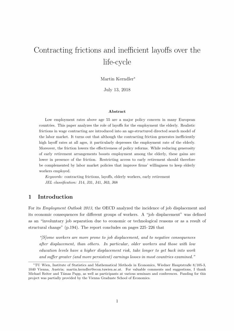
search andmatching
productivitydraw
endog.layoffs
productionand wages
exogenousseparation
σ
inactivityshockδ
agingshockπi
employed workers only
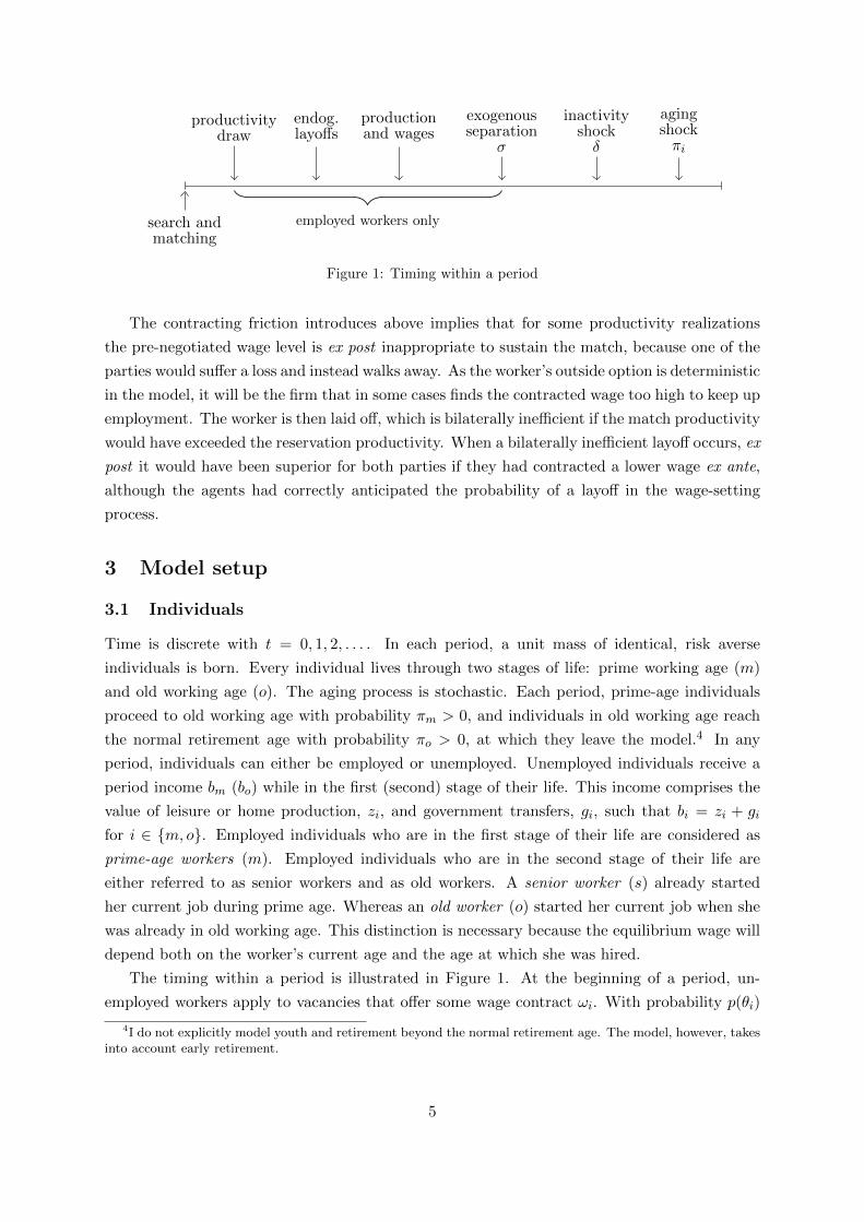
Figure 1: Timing within a period
The contracting friction introduces above implies that for some productivity realizations
the pre-negotiated wage level is ex post inappropriate to sustain the match, because one of the
parties would suffer a loss and instead walks away. As the worker’s outside option is deterministic
in the model, it will be the firm that in some cases finds the contracted wage too high to keep up
employment. The worker is then laid off, which is bilaterally inefficient if the match productivity
would have exceeded the reservation productivity. When a bilaterally inefficient layoff occurs, ex
post it would have been superior for both parties if they had contracted a lower wage ex ante,
although the agents had correctly anticipated the probability of a layoff in the wage-setting
process.
3 Model setup
3.1 Individuals
Time is discrete with t = 0, 1, 2, . . . . In each period, a unit mass of identical, risk averse
individuals is born. Every individual lives through two stages of life: prime working age (m)
and old working age (o). The aging process is stochastic. Each period, prime-age individuals
proceed to old working age with probability πm > 0, and individuals in old working age reach
the normal retirement age with probability πo > 0, at which they leave the model.4 In any
period, individuals can either be employed or unemployed. Unemployed individuals receive a
period income bm (bo) while in the first (second) stage of their life. This income comprises the
value of leisure or home production, zi, and government transfers, gi, such that bi = zi + gi
for i ∈ {m, o}. Employed individuals who are in the first stage of their life are considered as
prime-age workers (m). Employed individuals who are in the second stage of their life are
either referred to as senior workers and as old workers. A senior worker (s) already started
her current job during prime age. Whereas an old worker (o) started her current job when she
was already in old working age. This distinction is necessary because the equilibrium wage will
depend both on the worker’s current age and the age at which she was hired.
The timing within a period is illustrated in Figure 1. At the beginning of a period, un-
employed workers apply to vacancies that offer some wage contract ωi. With probability p(θi)
4I do not explicitly model youth and retirement beyond the normal retirement age. The model, however, takesinto account early retirement.
5
this application is successful, and a new firm–worker match is formed. Firm and worker then
commit to the wage contract but not to actual employment. That is, either party can leave the
match at any time.
The period output yi that a matched worker can generate is stochastic and emerges from a
distribution that may depend on the worker type i ∈ {m, s, o}. Productivity is drawn at the
beginning of a match and renewed when the aging shock hits. In any other period, a new draw
happens with probability φ ∈ [0, 1]. The draws are independent across individuals, periods,
and age groups. After the productivity of the current period is observed by the firm, it may
terminate the match. Doing so is optimal if the firm surplus from the match turns out to be
negative, that is, if the wage stream promised to the worker exceeds the sum of today’s output
and expected future output. If the match is profitable for the firm, production takes place and
wages are paid according to the specified contract ωi.
After the production stage, the match ends for exogenous reasons with probability σ ≥0. Old individuals (regardless of their employment status) may additionally experience an
inactivity shock with probability δ ≥ 0, after which they do not participate in the labor market
any more. That is, they permanently stop all work and search activities. This could, for
instance, capture a health shock that destroys the worker’s production capacity, or a labor
market exit for non-economic reasons. The aging shock hits at the very end of the period.
3.2 Productivity
The productivity of a match with a type i worker is a realization of the random variable Yi for
i ∈ {m, s, o}. These random variables satisfy some general properties.
Assumption 1. Denote the distribution function of Yi as Fi for i ∈ {m, s, o}. The distribution
functions differ only in terms of a location parameter µi ∈ R, a scale parameter si > 0, and a
shape parameter αi > 0. In particular, there exists a random variable Z with cdf F such that
Fi(y) = F(y−µi
si
)αi for i ∈ {m, s, o} and the following properties hold:
(i) the cdf F is twice continuously differentiable, the associated density f has support on the
whole real line,
(ii) the random variable Z satisfies 0 ≤ EZ <∞,
(iii) the hazard rate h := f1−F is strictly increasing, while h′
h is non-increasing,
(iv) the conditional expectation E[Z − a|Z ≥ a] is convex in a.
According to the first part of the assumption, the three distribution functions are members
of the same family of parametric distributions. For given shape parameter αi, this is a location-
scale family. The parameter µi governs the mean of the distribution, while si governs its
dispersion. Prominent examples for such families are the normal distribution family and the
logistic distribution family. To control the skewness of the distribution, I additionally introduce
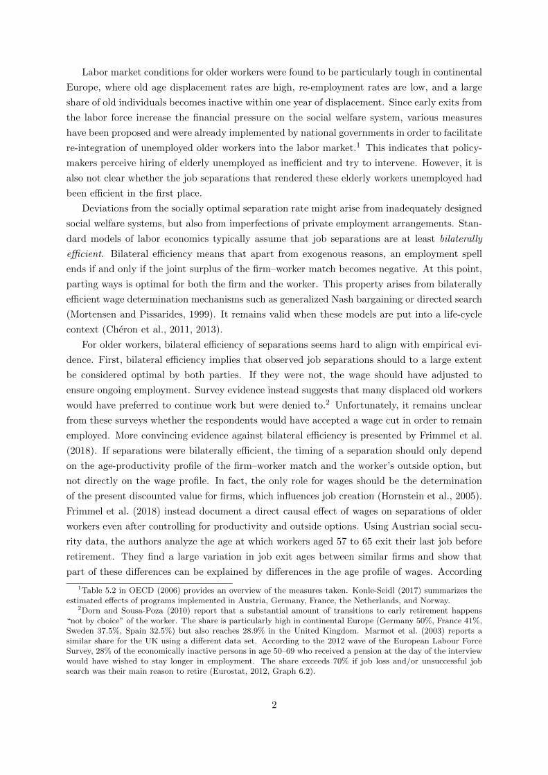
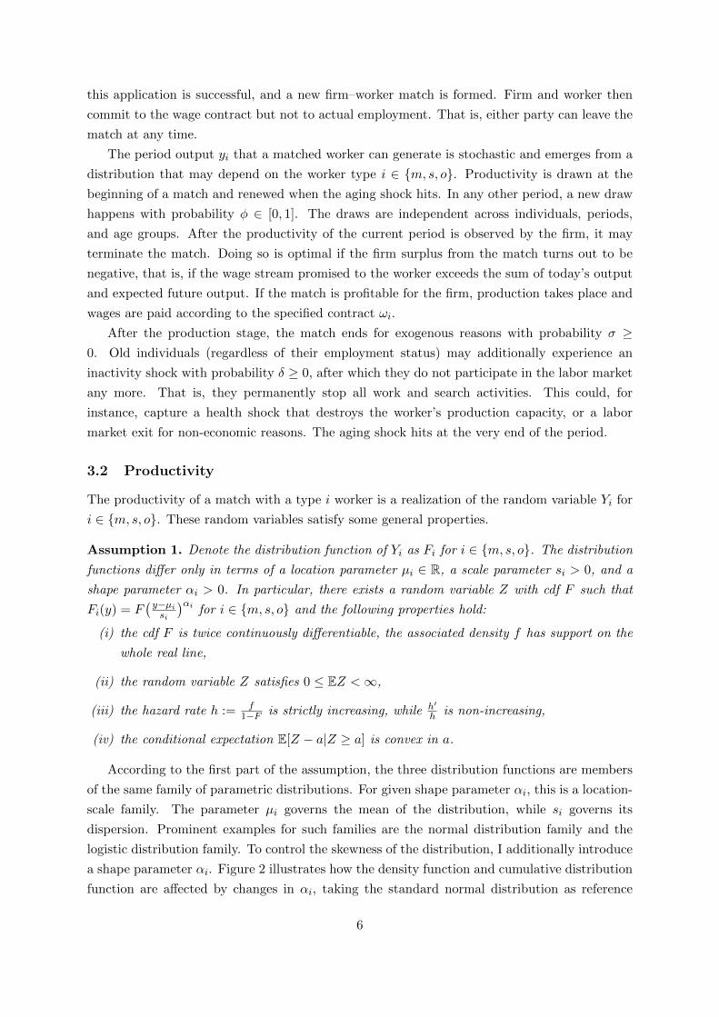
a shape parameter αi. Figure 2 illustrates how the density function and cumulative distribution
function are affected by changes in αi, taking the standard normal distribution as reference
6
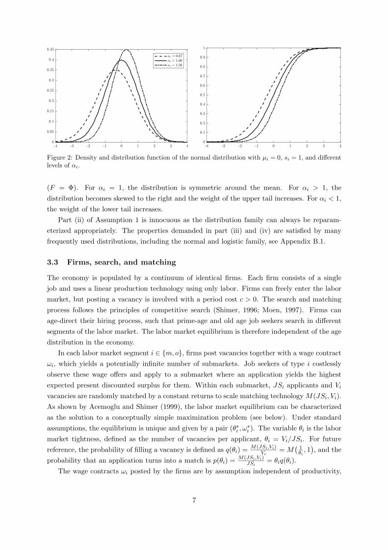
Figure 2: Density and distribution function of the normal distribution with µi = 0, si = 1, and differentlevels of αi.
(F = Φ). For αi = 1, the distribution is symmetric around the mean. For αi > 1, the
distribution becomes skewed to the right and the weight of the upper tail increases. For αi < 1,
the weight of the lower tail increases.
Part (ii) of Assumption 1 is innocuous as the distribution family can always be reparam-
eterized appropriately. The properties demanded in part (iii) and (iv) are satisfied by many
frequently used distributions, including the normal and logistic family, see Appendix B.1.
3.3 Firms, search, and matching
The economy is populated by a continuum of identical firms. Each firm consists of a single
job and uses a linear production technology using only labor. Firms can freely enter the labor
market, but posting a vacancy is involved with a period cost c > 0. The search and matching
process follows the principles of competitive search (Shimer, 1996; Moen, 1997). Firms can
age-direct their hiring process, such that prime-age and old age job seekers search in different
segments of the labor market. The labor market equilibrium is therefore independent of the age
distribution in the economy.
In each labor market segment i ∈ {m, o}, firms post vacancies together with a wage contract
ωi, which yields a potentially infinite number of submarkets. Job seekers of type i costlessly
observe these wage offers and apply to a submarket where an application yields the highest
expected present discounted surplus for them. Within each submarket, JSi applicants and Vi
vacancies are randomly matched by a constant returns to scale matching technology M(JSi, Vi).
As shown by Acemoglu and Shimer (1999), the labor market equilibrium can be characterized
as the solution to a conceptually simple maximization problem (see below). Under standard
assumptions, the equilibrium is unique and given by a pair (θ∗i , ω∗i ). The variable θi is the labor
market tightness, defined as the number of vacancies per applicant, θi = Vi/JSi. For future
reference, the probability of filling a vacancy is defined as q(θi) = M(JSi,Vi)Vi
= M(
1θi, 1), and the
probability that an application turns into a match is p(θi) = M(JSi,Vi)JSi
= θiq(θi).
The wage contracts ωi posted by the firms are by assumption independent of productivity,
7

but may depend on the worker’s age. Therefore, prime-age job seekers look for wage contracts
that specify a pair of wages ωm = (wm, ws). The wage wm applies as long as the worker is in
prime working age, and the wage ws applies thereafter. The contracts offered to old job seekers
specify a single wage, ωo = (wo).
3.4 Government
The government plays a passive role in the model. The transfers gi that non-employment
individuals receive are financed by a lump sum tax τ levied on the whole population. In Section 6
I allow for additional government spending and/or revenue from labor market policies.
4 Equilibrium with the contracting friction
The model is solved assuming a demographic and economic steady state. The equilibrium
consists of a set of wage contracts (ω∗m, ω∗o), labor market tightnesses (θ∗m, θ
∗o), search values
(Vm, Vo), and a lump sum tax τ∗ that satisfy the following conditions:
(1) labor market equilibrium of old job seekers, i.e. taking τ∗ and (θ∗m, ω∗m, Vm) as given, the
triple (θ∗o , ω∗o , Vo) forms a directed search equilibrium:
• firms maximize profit under free entry, q(θ∗o)EJ+o (ω∗o) = c,
• job seekers apply optimally, Vo = max(θo,ωo) p(θo)EW+o (ωo) ≥ p(θ∗o)EW+
o (ω∗o),
(2) labor market equilibrium of prime-age job seekers, i.e. taking τ∗ and (θ∗o , ω∗o , Vo) as given,
the triple (θ∗m, ω∗m, Vm) forms a directed search equilibrium:
• firms maximize profit under free entry, q(θ∗m)EJ+m(ω∗m) = c,
• job seekers apply optimally, Vm = max(θm,ωm) p(θm)EW+m(ωm) ≥ p(θ∗m)EW+
m(ω∗m),
(3) balanced budget, i.e. taking (θ∗o , ω∗o , Vo) and (θ∗m, ω
∗m, Vm) as given, τ∗ balances the govern-
ment budget.
Due to directed search, the labor market equilibrium on the labor market of old job seekers
actually does not depend on (θ∗m, ω∗m, Vm). The labor market equilibria can therefore be solved
recursively. Section 4.1 considers the labor market equilibrium of old job seekers, before I turn
to prime-age job seekers in Section 4.2. Section 4.3 defines aggregate economic measures and
the equilibrium tax level. The analysis proceeds under the following functional restrictions:
Assumption 2. Firms are risk neutral. Workers are risk averse with instantaneous utility
function u defined on the interval (d,∞) where d ∈ R ∪ {−∞} and limx→d u(x) = −∞. It is
three times differentiable with u′ > 0, u′′ < 0, u′′′ ≥ 0, and limx→∞ u′(x) = 0. The matching
function is Cobb-Douglas, which implies q(θ) = Aθ−γ where A > 0 and γ ∈ (0, 1).
The assumptions on the utility function encompass, for example, the CARA and CRRA
specifications. The specific form of the matching function makes the analysis of comparative
8
static effects more tractable. The main results of the paper also hold for more general matching
functions with varying matching elasticity ε(θ) = − q′(θ)θq(θ) . The main advantage of a constant
elasticity ε(θ) = γ is that the optimal wage contract does not depend on the labor market
tightness.
For the sake of tractability, the shape parameter of the distribution function is set to αi = 1
throughout this section.
Assumption 3. Assume that αi = 1 for all i ∈ {m, s, o}.
Under Assumption 3, the monotonicity properties of the hazard rate h demanded by As-
sumption 1 also apply to the hazard rates of the productivity distributions Yi, that are given
by hi := fi1−Fi for i ∈ {m, s, o}.
4.1 Labor market equilibrium of old job seekers
Following Acemoglu and Shimer (1999), the labor market equilibrium on the labor market of
old job seekers is characterized as the solution to the constrained maximization problem
Vo := max(θo,wo)
p(θo)EW+o (wo) s.t. q(θo)EJ+
o (wo) = c. (1)
Intuitively, an old unemployed individual maximizes her expected surplus from applying to
a vacancy with characteristics (θo, wo), which is p(θo)EW+o (wo). With probability p(θo), the
application is successful and generates an expected worker surplus of EW+o (wo). Otherwise,
the individual remains unemployed and her surplus over unemployment is zero by definition.
Due to free entry, the value of vacant job is zero in equilibrium, such that the expected firm
surplus of posting a vacancy just makes up for the posting cost c. This gives rise to the free
entry condition q(θo)EJ+o (wo) = c, where q(θo) is the probability that the vacancy turns into a
match, and EJ+o (wo) denotes the expected firm surplus of this match.
At the production stage, firm and worker surplus evolve over time according to
Jo(wo; y) = y − wo + βo[φEJ+o (wo) + (1− φ)Jo(wo; y)], (2)
Wo(wo) = u(wo − τ)− u(bo − τ) + βo[φEW+o (wo) + (1− φ)Wo(wo)− Vo], (3)
where βo := β(1 − πo)(1 − σ)(1 − δ) is the effective time discount factor and β ∈ [0, 1) is the
pure time discount factor. Since the model is solved in a steady state, time indices are dropped
altogether. The firm surplus Jo(wo; y) comprises the instantaneous profit y − wo and future
profits discounted with the effective discount factor βo. With probability φ a new productivity
is drawn next period, which generates an expected surplus of EJ+o (wo). With probability 1−φ,
the current draw prevails, and the surplus is the same as in the current period. The same logic
applies to the surplus function of the worker. The instantaneous surplus over unemployment
is captured by the difference in utility u(wo − τ) − u(bo − τ) where τ is the lump sum tax.
The continuation value of the match is diminished by the value of search Vo that unemployed
workers pursue in the next period (employed workers do not search on the job).
9
At the layoff stage, the worker is dismissed if and only if firm surplus is negative, Jo(wo; y) <
0. This can be rewritten in the form y < yo(wo) := wo − βoφEJ+
o , where yo(wo) is the layoff
threshold. In case of a layoff, the firm is left with a vacant job, which generates a value of zero.
Taking this into account, firm surplus at the search stage is EJ+o (wo) =
∫∞yo(wo)
Jo(wo; y) dFo(y).
By equation (2), Jo(wo; y) =y−y
o(wo)
1−βo(1−φ) , and therefore the layoff threshold solves
yo− wo +
βoφ
1− βo(1− φ)
∫ ∞yo
y − yodFo(y) = 0. (4)
The following proposition establishes that the layoff threshold is well-defined, and how it reacts
to marginal changes in the model parameters.
Proposition 1. For any wo ∈ R, equation (4) uniquely defines a layoff threshold yo. The layoff
threshold is increasing in wo and decreasing in βo, φ, µo, and so.
The proof of this proposition and all other propositions can be found in Appendix B.3.
Ceteris paribus, a higher wage decreases firm profit such that a higher productivity level is
necessary for the firm to break even. The remaining parameters examined in Proposition 1 all
increase future expected firm profit, and therefore the firm is willing to accept lower profits today.
For future reference, define expected firm surplus conditional on retention as Jo(yo(wo)) =
E[Jo(wo;Yo)|Yo ≥ yo(wo)] =
E[Yo−yo(wo)|Yo≥yo(wo)]1−βo(1−φ) , which only depends on wo via the layoff
threshold yo(wo). To simplify notation, dependence of y
oon the wage is omitted in the following.
Expected worker surplus at the search stage is EW+o (wo) = (1−Fo(yo))Wo(wo). Substituting
this back into (3) yields Wo(wo) = u(wo−τ)−u(bo−τ)−βoVo1−βo(1−φFo(yo))
. In her optimal application decision,
the worker takes the value Vo as given. Yet, in equilibrium Vo = p(θ∗o)EW+o (w∗o) must hold.5
4.1.1 Equilibrium conditions
The first order optimality conditions of problem (1) can be summarized as
u′(w∗o − τ) =1− γγ
Wo(w∗o)
Jo(y∗o)+ (1− βo(1− φ))ho(y
∗o)∂y∗
o
∂woWo(w
∗o), (5)
q(θ∗o)EJ+o (w∗o) = c, (6)
where y∗o
= yo(w∗o) is defined in (4). The left-hand side of equation (5) captures the utility gain
from a marginally higher wage, whereas the right-hand side combines the marginal costs of a
higher wage. The first term on the right-hand side is standard in the literature and reflects the
search friction. The higher the wage, the lower the worker’s probability of finding a job. The
second term on the right-hand side is novel and stems from the contracting friction. In case of
a layoff, the worker loses the match surplus Wo(w∗o). The product Ho(wo) = ho(yo)
∂yo
∂woreflects
the link between wage level and job security. It combines the marginal effect of wo on the firm’s
5Since the worker’s reservation wage is independent of match productivity, the possibility of voluntary quitscan be safely ignored.
10
layoff threshold yo, measured by the partial derivativey∗o
∂wo= 1−βo(1−φ)
1−βo(1−φFo(y∗o)) > 0, and the hazard
rate ho(y∗o). The latter determines how sensitive the retention probability responds to a change
in the layoff threshold, since in general terms ho(x) = fo(x)1−Fo(x) = −∂ ln(1−Fo(x))
∂x . The product
Ho(wo) can therefore be interpreted as the marginal rate of substitution between the wage wo
and the log probability of retention ln(1 − Fo(yo)). If Ho(wo) = 0, the retention probability is
inelastic to the wage and the worker does not act against the risk. In this case, condition (5)
implies that the worker earns a share γ of the joint surplus of employment Wo(w∗o)u′(w∗o−τ) + Jo(y
∗o).
This is the usual finding when bargaining is bilaterally efficient as in Acemoglu and Shimer
(1999). With Ho(wo) > 0 it is no longer true. The higher Ho(wo), the more the worker is
willing to decrease her wage in favor of a higher retention probability. This reduces the worker’s
share in match surplus below γ, and the firm earns an additional rent.6
The labor market equilibrium on the labor market of the old job seekers is characterized by
the conditions (4)–(6), together with Vo = p(θ∗o)EW+o (w∗o). For the special case that old age
lasts for one period only (πo = 1), existence and uniqueness of a labor market equilibrium can
be established analytically. The threshold productivity then equals the wage, yo(wo) = wo, and
the worker’s reservation wage is her unemployment income bo.
Proposition 2. Let πo = 1. For given tax level τ , a unique labor market equilibrium of old job
seekers (θ∗o , w∗o , Vo) exists and satisfies w∗o > bo.
Since the optimal wage w∗o exceeds the worker’s reservation wage bo, part of the layoffs that
occur in equilibrium are bilaterally inefficient. If the informational friction could be overcome,
it would be optimal to maintain all matches with productivity Yo ≥ bo, because in this case the
value the individual generates in employment exceeds the value of non-employment. Due to the
contracting friction, however, also matches with Yo ∈ (bo, w∗o) are dissolved because of negative
firm profit. The probability for such a bilaterally inefficient layoff is Fo(w∗o)− Fo(bo).
4.1.2 Comparative static effects
To obtain comparative static effects, I continue to assume that old age lasts for one period only,
πo = 1. Equation (5) then can be expressed as
Φ(w∗o) = u′(w∗o − τ)− 1− γγ
Wo(w∗o)
Jo(w∗o)− ho(w∗o)Wo(w
∗o) = 0, (7)
where Wo(wo) = u(wo − τ) − u(bo − τ) and Jo(wo) = E[Yo − wo|Yo ≥ wo] since yo(wo) = wo.
A marginal change in one of the model parameters in general spurs two effects to which the
worker responds. The first effect, which I refer to as income effect (IE) captures the worker’s
reaction to changes in the surplus functions Wo and Jo, and the distribution function Fo. The
6This is similar to the informational rent highlighted by Kennan (2010). Lemma B.2(i) can be used to showthat the optimal worker share in surplus always lies in the interval ( γ
1+γ, γ).
11
income effect of an arbitrary parameter ξ on the equilibrium wage is(∂w∗o∂ξ
)IE= −Φ′(w∗o)
−1
{1− γγ
Wo(w∗o)
Jo(w∗o)2
∂Jo(w∗o)
∂ξ−[
1− γγ
1
Jo(w∗o)+ ho(w
∗o)
]∂Wo(w
∗o)
∂ξ
}where Φ′(w∗o) < 0. In absence of a contracting friction, only this income effect occurs. With a
contracting friction, however, also the worker’s valuation of risk may change. This corresponds
to a change in the hazard function ho on the right-hand side of (7) and triggers a substitution
effect (SE), (∂w∗o∂ξ
)SE= Φ′(w∗o)
−1∂ho(w∗o)
∂ξWo(w
∗o).
The marginal effect of an arbitrary parameter ξ on the equilibrium layoff probability is
dFo(w∗o)
dξ=∂Fo(w
∗o)
∂ξ+ fo(w
∗o)∂w∗o∂ξ
=∂Fo(w
∗o)
∂ξ+ fo(w
∗o)
(∂w∗o∂ξ
)IE︸ ︷︷ ︸
IE
+fo(w∗o)
(∂w∗o∂ξ
)SE︸ ︷︷ ︸
SE
. (8)
It combines the direct effect of ξ on the productivity distribution and the indirect effect through
the equilibrium wage w∗o . By the free entry condition (6), the equilibrium job-finding probability
is determined by expected firm surplus EJ+o (w∗o). Higher expected surplus boosts vacancy-
posting, which increases the labor market tightness θ∗o and the job-finding probability p(θ∗o).
Expected firm surplus is also affected by parameter changes through a direct distributional
effect and an indirect wage effect,
dEJ+o (w∗o)
dξ= −
∫ ∞w∗o
∂Fo(y)
∂ξdy − (1− Fo(w∗o))
∂w∗o∂ξ
(9)
= −∫ ∞w∗o
∂Fo(y)
∂ξdy − (1− Fo(w∗o))
(∂w∗o∂ξ
)IE︸ ︷︷ ︸
IE
−(1− Fo(w∗o))(∂w∗o∂ξ
)SE︸ ︷︷ ︸
SE
.
From the above expressions it is easy to see how a change in the worker’s valuation of risk, ho,
affects the labor market equilibrium through the substitution effects. If the retention probability
becomes locally more sensitive to the wage, ∂ho(w∗o)
∂ξ > 0, the worker substitutes away from wage
income in favor of a higher retention probability and a higher job-finding probability. The
opposite happens if ∂ho(w∗o)∂ξ < 0. In the following, I illustrate the comparative static effects of
the most relevant model parameters.
Unemployment income. An increase in bo, for instance due to higher unemployment or
early retirement benefits, lowers worker surplus Wo. Because the productivity distribution is
unaffected, there is no change in Jo and ho, and also no substitution effect. The income effect
increases the equilibrium wage since the worker’s outside option improves. This increases the
layoff probability and lowers the job-finding probability.
12
Old age productivity. The productivity parameters µo and so affect expected firm surplus
and the hazard function, but not worker surplus. The sign of the partial derivatives of ho and
Jo are established in Lemma B.1 and Lemma B.2 in Appendix B, respectively. An increase in
the location parameter µo shifts the productivity distribution to the right, which raises firm
surplus and lowers the hazard for given wage. Both the higher productivity (IE) and the lower
valuation of risk (SE) increase the equilibrium wage. Furthermore, the distribution function
decreases for given wage, ∂Fo(w∗o)∂µo
= −fo(w∗o) < 0. Proposition 3 establishes that this negative
direct effect dominates the positive wage effect in (8) and (9) because the wage increase is less
than proportional, ∂w∗o∂µo
< 1. As a result, the equilibrium layoff probability decreases and the
job-finding probability increases when the productivity distribution shifts to the right.
Proposition 3. A marginal increase in the location parameter µo increases the equilibrium
wage w∗o, lowers the layoff probability Fo(w∗o), and increases the job-finding probability p(θ∗o).
An increase in the scale parameter so has potentially ambiguous effects on the labor market
equilibrium. Under additional assumptions, however, it is possible to derive analytical results.
Proposition 4. A marginal increase in the scale parameter so exerts a positive income effect
on w∗o. The substitution effect is positive if and only if w∗o−µoso
> z, where z < 0 is the unique
root of h(z) + h′(z)z.
Assume that w∗o ≤ µo. Then the layoff probability increases in so, and the job-finding
probability increases if either ∂w∗o∂so≤ 0 or γ ≤ Jo(w∗o)+w∗o−µo
Jo(w∗o)+[1−Jo(w∗o)ho(w∗o)](w∗o−µo).
Wage. The firm benefits from a more dispersed productivity distribution because the mass
of very productive workers is increasing, while the increasing mass of unproductive workers
is laid off at no cost. As a result, the average productivity per retained worker increases,∂Jo(w∗o)∂so
> 0, generating a positive income effect on w∗o . The substitution effect can be positive
or negative, depending on the reaction of the hazard function. For w∗o−µoso
< z, the hazard
function increases as the retention probability 1 − Fo becomes locally more sensitive to the
wage (cf. Lemma B.1). In response, workers are willing to give up part of their wage in favor
of higher job security. However, if wages are sufficiently high such that w∗o−µoso
> z, increasing
uncertainty actually decreases the willingness to substitute wages for job security because the
retention rate becomes locally less responsive to the wage. This non-monotonic behavior occurs
because an increase in so makes the distribution function steeper at the tails of the distribution,
while it becomes flatter in the middle. The equilibrium wage therefore unambiguously increases
if w∗o−µoso
> z, while the wage response is analytically not clear otherwise.
Layoffs. A higher scale parameter so increases the distribution function for w∗o ≤ µo and
decreases it for w∗o ≥ µo. I consider the first case more relevant for real world applications,
such that ∂Fo(w∗o)∂so
= −w∗o−µos2o
fo(w∗o) ≥ 0. It can be shown that under this condition, the
positive income effect always offsets the potentially negative substitution effect in (8), such
that the equilibrium layoff probability increases. Therefore, even if the worker responds to
higher uncertainty by contracting a lower wage, layoffs become more likely.
13
Hiring. The direct effect of so on the job-finding probability is positive, since−∫∞w∗o
∂Fo(y)∂so
dy =1−Fo(w∗o)
so[Jo(w
∗o) + w∗o − µo] ≥ 0 (see proof of Proposition 4). Intuitively, the higher expected
productivity per retained worker more than compensates the firm for the lower retention proba-
bility of the workers. If the equilibrium wage decreases in so, this further increases firm surplus,
and the job-finding probability unambiguously increases as evident from (9). If ∂w∗o∂so
> 0, the
upper boundary on γ established by Proposition 4 ensures that the wage increase does not
offset the direct distributional effect. Intuitively, the lower γ, the more of the additional match
surplus per retained worker is captured by the firm, and the less the equilibrium wage increases.
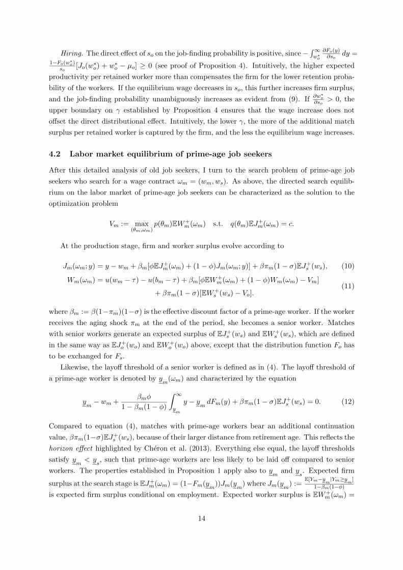
4.2 Labor market equilibrium of prime-age job seekers
After this detailed analysis of old job seekers, I turn to the search problem of prime-age job
seekers who search for a wage contract ωm = (wm, ws). As above, the directed search equilib-
rium on the labor market of prime-age job seekers can be characterized as the solution to the
optimization problem
Vm := max(θm,ωm)
p(θm)EW+m(ωm) s.t. q(θm)EJ+
m(ωm) = c.
At the production stage, firm and worker surplus evolve according to
Jm(ωm; y) = y − wm + βm[φEJ+m(ωm) + (1− φ)Jm(ωm; y)] + βπm(1− σ)EJ+
s (ws), (10)
Wm(ωm) = u(wm − τ)− u(bm − τ) + βm[φEW+m(ωm) + (1− φ)Wm(ωm)− Vm]
+ βπm(1− σ)[EW+s (ws)− Vo].
(11)
where βm := β(1−πm)(1−σ) is the effective discount factor of a prime-age worker. If the worker
receives the aging shock πm at the end of the period, she becomes a senior worker. Matches
with senior workers generate an expected surplus of EJ+s (ws) and EW+
s (ws), which are defined
in the same way as EJ+o (wo) and EW+
o (wo) above, except that the distribution function Fo has
to be exchanged for Fs.
Likewise, the layoff threshold of a senior worker is defined as in (4). The layoff threshold of
a prime-age worker is denoted by ym
(ωm) and characterized by the equation
ym− wm +
βmφ
1− βm(1− φ)
∫ ∞ym
y − ymdFm(y) + βπm(1− σ)EJ+
s (ws) = 0. (12)
Compared to equation (4), matches with prime-age workers bear an additional continuation
value, βπm(1−σ)EJ+s (ws), because of their larger distance from retirement age. This reflects the
horizon effect highlighted by Cheron et al. (2013). Everything else equal, the layoff thresholds
satisfy ym< y
s, such that prime-age workers are less likely to be laid off compared to senior
workers. The properties established in Proposition 1 apply also to ym
and ys. Expected firm
surplus at the search stage is EJ+m(ωm) = (1−Fm(y
m))Jm(y
m) where Jm(y
m) :=
E[Ym−ym|Ym≥ym]
1−βm(1−φ)
is expected firm surplus conditional on employment. Expected worker surplus is EW+m(ωm) =
14
(1− Fm(ym
))Wm(ωm) where Wm(ωm) = u(wm−τ)−u(bm−τ)−βmVm+βπm(1−σ)[EW+s (ws)−Vo]
1−βm(1−φFm(ym
)) .
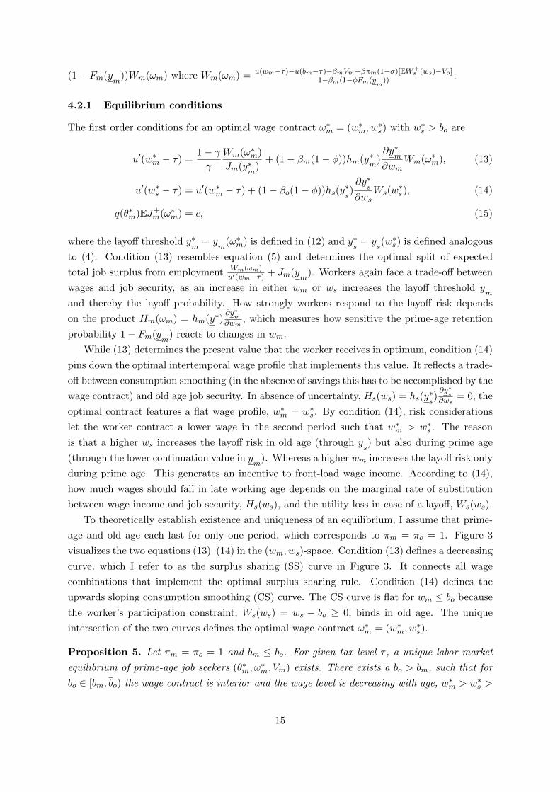
4.2.1 Equilibrium conditions
The first order conditions for an optimal wage contract ω∗m = (w∗m, w∗s) with w∗s > bo are
u′(w∗m − τ) =1− γγ
Wm(ω∗m)
Jm(y∗m
)+ (1− βm(1− φ))hm(y∗
m)∂y∗
m
∂wmWm(ω∗m), (13)
u′(w∗s − τ) = u′(w∗m − τ) + (1− βo(1− φ))hs(y∗s)∂y∗
s
∂wsWs(w
∗s), (14)
q(θ∗m)EJ+m(ω∗m) = c, (15)
where the layoff threshold y∗m
= ym
(ω∗m) is defined in (12) and y∗s
= ys(w∗s) is defined analogous
to (4). Condition (13) resembles equation (5) and determines the optimal split of expected
total job surplus from employment Wm(ωm)u′(wm−τ) + Jm(y
m). Workers again face a trade-off between
wages and job security, as an increase in either wm or ws increases the layoff threshold ym
and thereby the layoff probability. How strongly workers respond to the layoff risk depends
on the product Hm(ωm) = hm(y∗)∂y∗m
∂wm, which measures how sensitive the prime-age retention
probability 1− Fm(ym
) reacts to changes in wm.
While (13) determines the present value that the worker receives in optimum, condition (14)
pins down the optimal intertemporal wage profile that implements this value. It reflects a trade-
off between consumption smoothing (in the absence of savings this has to be accomplished by the
wage contract) and old age job security. In absence of uncertainty, Hs(ws) = hs(y∗s)∂y∗s
∂ws= 0, the
optimal contract features a flat wage profile, w∗m = w∗s . By condition (14), risk considerations
let the worker contract a lower wage in the second period such that w∗m > w∗s . The reason
is that a higher ws increases the layoff risk in old age (through ys) but also during prime age
(through the lower continuation value in ym
). Whereas a higher wm increases the layoff risk only
during prime age. This generates an incentive to front-load wage income. According to (14),
how much wages should fall in late working age depends on the marginal rate of substitution
between wage income and job security, Hs(ws), and the utility loss in case of a layoff, Ws(ws).
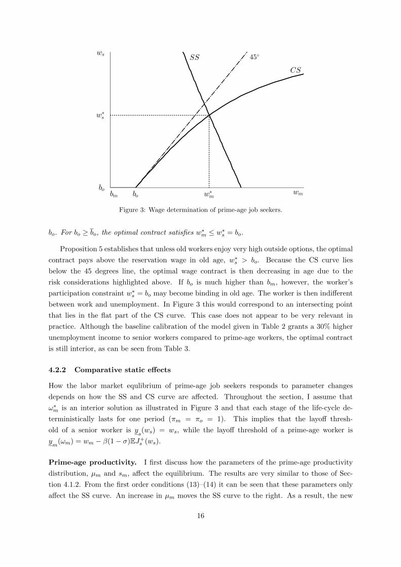
To theoretically establish existence and uniqueness of an equilibrium, I assume that prime-
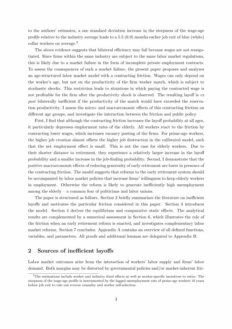
age and old age each last for only one period, which corresponds to πm = πo = 1. Figure 3
visualizes the two equations (13)–(14) in the (wm, ws)-space. Condition (13) defines a decreasing
curve, which I refer to as the surplus sharing (SS) curve in Figure 3. It connects all wage
combinations that implement the optimal surplus sharing rule. Condition (14) defines the
upwards sloping consumption smoothing (CS) curve. The CS curve is flat for wm ≤ bo because
the worker’s participation constraint, Ws(ws) = ws − bo ≥ 0, binds in old age. The unique
intersection of the two curves defines the optimal wage contract ω∗m = (w∗m, w∗s).
Proposition 5. Let πm = πo = 1 and bm ≤ bo. For given tax level τ , a unique labor market
equilibrium of prime-age job seekers (θ∗m, ω∗m, Vm) exists. There exists a bo > bm, such that for
bo ∈ [bm, bo) the wage contract is interior and the wage level is decreasing with age, w∗m > w∗s >
15
bo
w∗
s
ws
bm bo w∗
mwm
CS
SS 45◦
Figure 3: Wage determination of prime-age job seekers.
bo. For bo ≥ bo, the optimal contract satisfies w∗m ≤ w∗s = bo.
Proposition 5 establishes that unless old workers enjoy very high outside options, the optimal
contract pays above the reservation wage in old age, w∗s > bo. Because the CS curve lies
below the 45 degrees line, the optimal wage contract is then decreasing in age due to the
risk considerations highlighted above. If bo is much higher than bm, however, the worker’s
participation constraint w∗s = bo may become binding in old age. The worker is then indifferent
between work and unemployment. In Figure 3 this would correspond to an intersecting point
that lies in the flat part of the CS curve. This case does not appear to be very relevant in
practice. Although the baseline calibration of the model given in Table 2 grants a 30% higher
unemployment income to senior workers compared to prime-age workers, the optimal contract
is still interior, as can be seen from Table 3.
4.2.2 Comparative static effects
How the labor market equlibrium of prime-age job seekers responds to parameter changes
depends on how the SS and CS curve are affected. Throughout the section, I assume that
ω∗m is an interior solution as illustrated in Figure 3 and that each stage of the life-cycle de-
terministically lasts for one period (πm = πo = 1). This implies that the layoff thresh-
old of a senior worker is ys(ws) = ws, while the layoff threshold of a prime-age worker is
ym
(ωm) = wm − β(1− σ)EJ+s (ws).
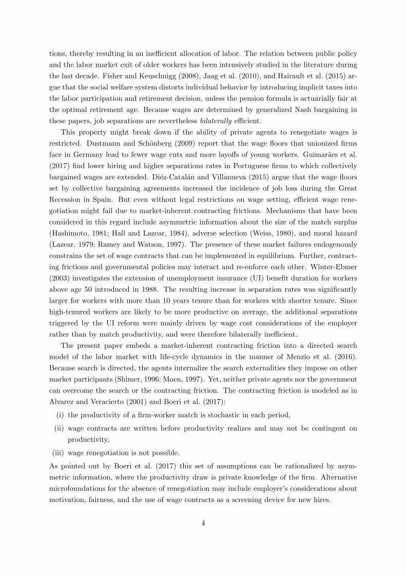
Prime-age productivity. I first discuss how the parameters of the prime-age productivity
distribution, µm and sm, affect the equilibrium. The results are very similar to those of Sec-
tion 4.1.2. From the first order conditions (13)–(14) it can be seen that these parameters only
affect the SS curve. An increase in µm moves the SS curve to the right. As a result, the new
16
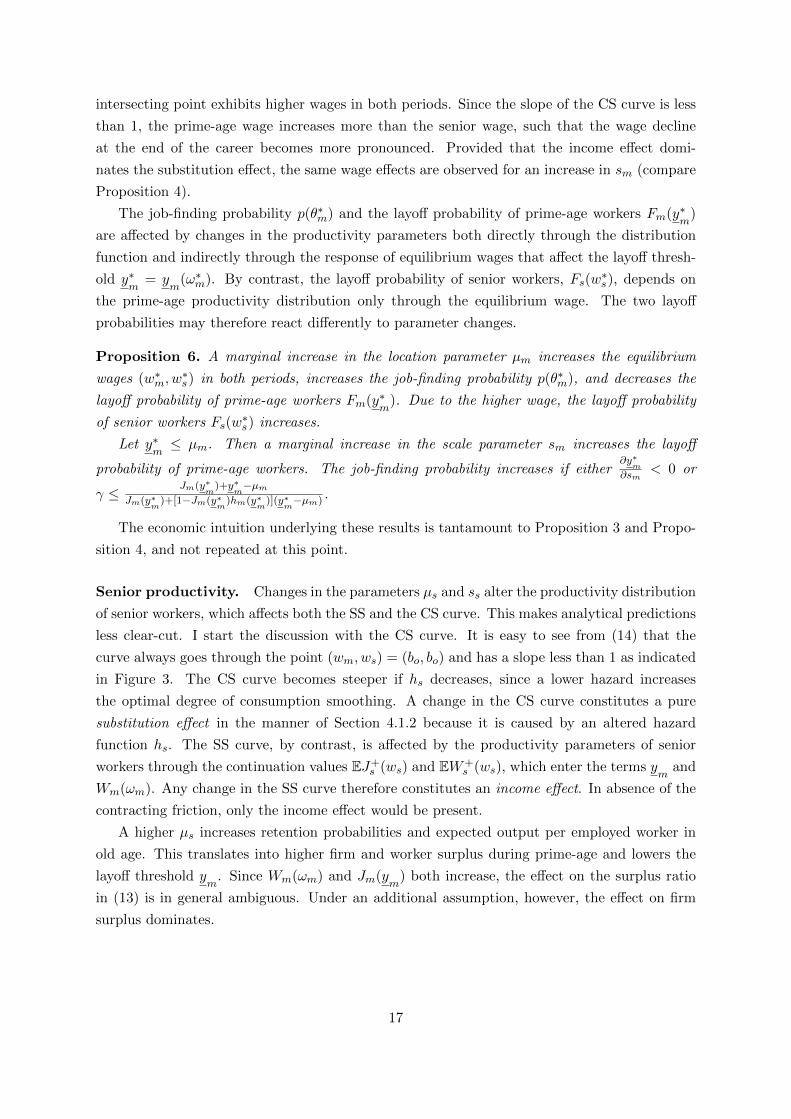
intersecting point exhibits higher wages in both periods. Since the slope of the CS curve is less
than 1, the prime-age wage increases more than the senior wage, such that the wage decline
at the end of the career becomes more pronounced. Provided that the income effect domi-
nates the substitution effect, the same wage effects are observed for an increase in sm (compare
Proposition 4).
The job-finding probability p(θ∗m) and the layoff probability of prime-age workers Fm(y∗m
)
are affected by changes in the productivity parameters both directly through the distribution
function and indirectly through the response of equilibrium wages that affect the layoff thresh-
old y∗m
= ym
(ω∗m). By contrast, the layoff probability of senior workers, Fs(w∗s), depends on
the prime-age productivity distribution only through the equilibrium wage. The two layoff
probabilities may therefore react differently to parameter changes.
Proposition 6. A marginal increase in the location parameter µm increases the equilibrium
wages (w∗m, w∗s) in both periods, increases the job-finding probability p(θ∗m), and decreases the
layoff probability of prime-age workers Fm(y∗m
). Due to the higher wage, the layoff probability
of senior workers Fs(w∗s) increases.
Let y∗m≤ µm. Then a marginal increase in the scale parameter sm increases the layoff
probability of prime-age workers. The job-finding probability increases if either∂y∗m
∂sm< 0 or
γ ≤ Jm(y∗m
)+y∗m−µm
Jm(y∗m
)+[1−Jm(y∗m
)hm(y∗m
)](y∗m−µm) .
The economic intuition underlying these results is tantamount to Proposition 3 and Propo-
sition 4, and not repeated at this point.
Senior productivity. Changes in the parameters µs and ss alter the productivity distribution
of senior workers, which affects both the SS and the CS curve. This makes analytical predictions
less clear-cut. I start the discussion with the CS curve. It is easy to see from (14) that the
curve always goes through the point (wm, ws) = (bo, bo) and has a slope less than 1 as indicated
in Figure 3. The CS curve becomes steeper if hs decreases, since a lower hazard increases
the optimal degree of consumption smoothing. A change in the CS curve constitutes a pure
substitution effect in the manner of Section 4.1.2 because it is caused by an altered hazard
function hs. The SS curve, by contrast, is affected by the productivity parameters of senior
workers through the continuation values EJ+s (ws) and EW+
s (ws), which enter the terms ym
and
Wm(ωm). Any change in the SS curve therefore constitutes an income effect. In absence of the
contracting friction, only the income effect would be present.
A higher µs increases retention probabilities and expected output per employed worker in
old age. This translates into higher firm and worker surplus during prime-age and lowers the
layoff threshold ym
. Since Wm(ωm) and Jm(ym
) both increase, the effect on the surplus ratio
in (13) is in general ambiguous. Under an additional assumption, however, the effect on firm
surplus dominates.
17
bo
w∗
s
ws
bo w∗
mwm
CSSS 45◦
Figure 4: Wage response to an increase in µs.
bo
w∗
s
ws
bo w∗
mwm
CS
SS 45◦
Figure 5: Wage response to an increase in ss.
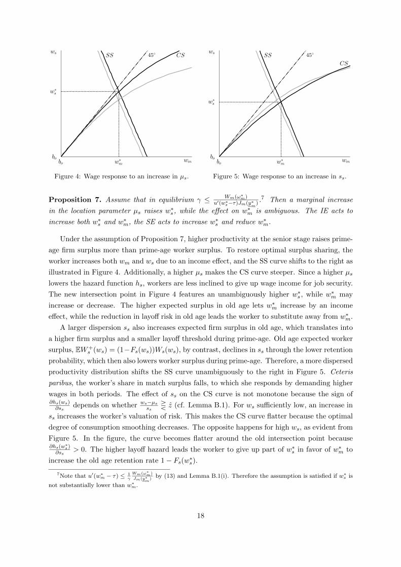
Proposition 7. Assume that in equilibrium γ ≤ Wm(ω∗m)u′(w∗s−τ)Jm(y∗
m) .7 Then a marginal increase
in the location parameter µs raises w∗s , while the effect on w∗m is ambiguous. The IE acts to
increase both w∗s and w∗m, the SE acts to increase w∗s and reduce w∗m.
Under the assumption of Proposition 7, higher productivity at the senior stage raises prime-
age firm surplus more than prime-age worker surplus. To restore optimal surplus sharing, the
worker increases both wm and ws due to an income effect, and the SS curve shifts to the right as
illustrated in Figure 4. Additionally, a higher µs makes the CS curve steeper. Since a higher µs
lowers the hazard function hs, workers are less inclined to give up wage income for job security.
The new intersection point in Figure 4 features an unambiguously higher w∗s , while w∗m may
increase or decrease. The higher expected surplus in old age lets w∗m increase by an income
effect, while the reduction in layoff risk in old age leads the worker to substitute away from w∗m.
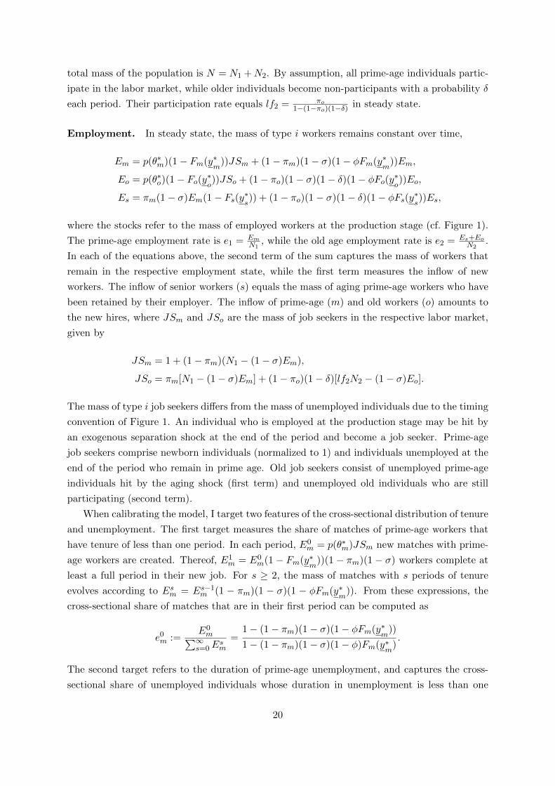
A larger dispersion ss also increases expected firm surplus in old age, which translates into
a higher firm surplus and a smaller layoff threshold during prime-age. Old age expected worker
surplus, EW+s (ws) = (1−Fs(ws))Ws(ws), by contrast, declines in ss through the lower retention
probability, which then also lowers worker surplus during prime-age. Therefore, a more dispersed
productivity distribution shifts the SS curve unambiguously to the right in Figure 5. Ceteris
paribus, the worker’s share in match surplus falls, to which she responds by demanding higher
wages in both periods. The effect of ss on the CS curve is not monotone because the sign of∂hs(ws)∂ss
depends on whether ws−µsss
R z (cf. Lemma B.1). For ws sufficiently low, an increase in
ss increases the worker’s valuation of risk. This makes the CS curve flatter because the optimal
degree of consumption smoothing decreases. The opposite happens for high ws, as evident from
Figure 5. In the figure, the curve becomes flatter around the old intersection point because∂hs(w∗s )∂ss
> 0. The higher layoff hazard leads the worker to give up part of w∗s in favor of w∗m to
increase the old age retention rate 1− Fs(w∗s).7Note that u′(w∗m − τ) ≤ 1
γ
Wm(ω∗m)
Jm(y∗m
)by (13) and Lemma B.1(i). Therefore the assumption is satisfied if w∗s is
not substantially lower than w∗m.
18

bo
w∗
s
ws
bo w∗
mwm
CS
SS 45◦
Figure 6: Wage response to an increase in bm.
bo
w∗
s
ws
bo w∗
mwm
CSSS 45◦
Figure 7: Wage response to an increase in bo.
Unemployment income. Since the unemployment incomes bm and bo do not affect the
hazard functions, the response of equilibrium wages is due to income effects that are driven by
changes in match surplus. A higher bm ceteris paribus decreases prime-age worker surplus due
to better outside options. To restore optimal surplus sharing, the worker increases wages in
both periods. This is captured by the outwards shift of the SS curve in Figure 6. Since bm does
not affect the CS curve, the new optimum exhibits a higher w∗m, a higher w∗s , and a lower ratio
w∗s/w∗m. The higher wages translate into higher layoff probabilities in both periods and a lower
job-finding probability.
Higher unemployment income for older workers, bo, has the same effect on the SS curve as
bm. Additionally, the CS curve moves upwards in Figure 7 because a layoff at the senior stage
becomes less costly for the worker. As a result, w∗s increases at the expense of w∗m. In total,
there are two upwards forces on w∗s , which unambiguously increases, accompanied by a higher
layoff probability in old age. The effect on the prime-age wage w∗m is not clear. As long as w∗m
does not substantially decrease, however, higher bo will also increase layoffs among prime-age
workers (through a higher y∗m
) and lower the job-finding probability.
Proposition 8. An increase in bm raises w∗m and w∗s , and lowers w∗s/w∗m. This increases layoff
probabilities for prime-age and senior workers, and lowers the job-finding probability p(θ∗m). An
increase in bo raises w∗s and thereby the layoff rate Fs(w∗s), while the effect on w∗m is ambiguous.
These observations suggest that a change in outside options of a certain age group has
stronger wage (and likely employment) effects on that age group, although workers are optimiz-
ing intertemporally.
4.3 Demography and economic aggregates
For simplicity, I assume a stationary demography. In each period, the inflow into an age group
equal its outflow. Since the mass of newborns is normalized to 1, in steady state there is as mass
N1 = 1πm
of prime-age individuals and a mass N2 = 1πo
of individuals in old working age. The
19
total mass of the population is N = N1 +N2. By assumption, all prime-age individuals partic-
ipate in the labor market, while older individuals become non-participants with a probability δ
each period. Their participation rate equals lf2 = πo1−(1−πo)(1−δ) in steady state.
Employment. In steady state, the mass of type i workers remains constant over time,
Em = p(θ∗m)(1− Fm(y∗m
))JSm + (1− πm)(1− σ)(1− φFm(y∗m
))Em,
Eo = p(θ∗o)(1− Fo(y∗o))JSo + (1− πo)(1− σ)(1− δ)(1− φFo(y∗o))Eo,
Es = πm(1− σ)Em(1− Fs(y∗s)) + (1− πo)(1− σ)(1− δ)(1− φFs(y∗s))Es,
where the stocks refer to the mass of employed workers at the production stage (cf. Figure 1).
The prime-age employment rate is e1 = EmN1
, while the old age employment rate is e2 = Es+EoN2
.
In each of the equations above, the second term of the sum captures the mass of workers that
remain in the respective employment state, while the first term measures the inflow of new
workers. The inflow of senior workers (s) equals the mass of aging prime-age workers who have
been retained by their employer. The inflow of prime-age (m) and old workers (o) amounts to
the new hires, where JSm and JSo are the mass of job seekers in the respective labor market,
given by
JSm = 1 + (1− πm)(N1 − (1− σ)Em),
JSo = πm[N1 − (1− σ)Em] + (1− πo)(1− δ)[lf2N2 − (1− σ)Eo].
The mass of type i job seekers differs from the mass of unemployed individuals due to the timing
convention of Figure 1. An individual who is employed at the production stage may be hit by
an exogenous separation shock at the end of the period and become a job seeker. Prime-age
job seekers comprise newborn individuals (normalized to 1) and individuals unemployed at the
end of the period who remain in prime age. Old job seekers consist of unemployed prime-age
individuals hit by the aging shock (first term) and unemployed old individuals who are still
participating (second term).
When calibrating the model, I target two features of the cross-sectional distribution of tenure
and unemployment. The first target measures the share of matches of prime-age workers that
have tenure of less than one period. In each period, E0m = p(θ∗m)JSm new matches with prime-
age workers are created. Thereof, E1m = E0
m(1− Fm(y∗m
))(1− πm)(1− σ) workers complete at
least a full period in their new job. For s ≥ 2, the mass of matches with s periods of tenure
evolves according to Esm = Es−1m (1 − πm)(1 − σ)(1 − φFm(y∗
m)). From these expressions, the
cross-sectional share of matches that are in their first period can be computed as
e0m :=
E0m∑∞
s=0Esm
=1− (1− πm)(1− σ)(1− φFm(y∗
m))
1− (1− πm)(1− σ)(1− φ)Fm(y∗m
).
The second target refers to the duration of prime-age unemployment, and captures the cross-
sectional share of unemployed individuals whose duration in unemployment is less than one
20
period. Unemployment spells are interrupted whenever a new match is formed, even if this
match is dissolved before the production stage. Since the period probability of staying prime-
age and unemployed is (1−p(θ∗m))(1−πm), the mass of workers with s periods of uninterrupted
unemployment satisfies U sm = U s−1m (1 − p(θ∗m))(1 − πm). The share of short-term unemployed
in all unemployed is therefore
u0m :=
U0m∑∞
s=0 Usm
= 1− (1− p(θ∗m))(1− πm).
Output. Output per age group is the value of produced goods net of vacancy posting costs,
Y1 = E[Ym|Ym ≥ y∗m]Em − cθ∗mJSm,
Y2 = E[Ys|Ys ≥ y∗s]Es + E[Yo|Yo ≥ y∗o]Eo − cθ∗oJSo.
Vacancy posting costs are subtracted from gross output as in Acemoglu and Shimer (1999),
because only the remainder acts to increase welfare in the economy (see below).
Government budget. The government provides transfers gm and go to unemployed prime-
age and old individuals, respectively. Aggregate public expenditures per age group are therefore
G1 = (N1 − Em)gm and G2 = (N2 − Es − Eo)go. The government collects a total tax revenue
of τN . The equilibrium tax level that balances the budget is thus τ∗ = G1+G2N .
Welfare. To quantify the welfare cost of the contracting friction, I define welfare as the sum
of utility within each age group,
W1 = Emu(w∗m − τ) + (N1 − Em)u(bm − τ),
W2 = Esu(w∗s − τ) + Eou(w∗o − τ) + (N2 − Eo − Es)u(bo − τ),
and total welfare asW =W1 +W2. Since firms earn zero expected profit, firm dividends can be
neglected altogether. To convert utility levels into consumption equivalents, I compute the per
capita income x that would generate the same level of welfare in the economy, i.e. Nu(x) =W.
This implies x = u−1(W/N).
5 Equilibrium without the contracting friction
To quantify the welfare and employment loss that is caused by the contracting friction, I com-
pare the equilibrium defined in Section 4 to the equilibrium of a counterfactual economy in
which wages can be productivity-contingent. In this economy, wage contracts specify wages
schedules wi : R→ R which can be arbitrary measurable functions of contemporaneous match
productivity. I maintain the assumption that employment only occurs if both parties receive
non-negative rents. Since wages can be productivity contingent, however, matches with positive
joint surplus are never destroyed endogenously in equilibrium. Therefore, layoffs are bilaterally
21
efficient, and the layoff threshold of the firm becomes the reservation productivity yri implicitly
defined by Wi(wi; yri ) = Ji(wi; y
ri ) = 0.
5.1 Labor market equilibrium of old job seekers
Firm and worker surplus at the production stage satisfy equations (2)–(3), except that wo has
to be replaced by wo(y). Expected firm and worker surplus at the search stage are
EJ+o (wo) =
∫ ∞yro
Jo(wo; y) dFo(y) =
∫∞yroy − wo(y) dFo(y)
1− βo(1− φFo(yro)),
EW+o (wo) =
∫ ∞yro
Wo(wo; y) dFo(y) =
∫∞yrou(wo(y)− τ)− u(bo − τ)− βoVo dFo(y)
1− βo(1− φFo(yro)).
Since Jo(wo; y) ≥ 0 requires wo(y) ≤ y + βoφEJ+o (wo), the reservation productivity yro where
both parties are indifferent between employment and non-employment satisfies
u(yro + βoφEJ+
o (wo)− τ)− u(bo − τ) + βoφEW+
o (wo)− βoVo = 0. (16)
The equilibrium on the labor market for old job seekers is characterized as in (1) but with the
additional condition that Jo(wo; y) ≥ 0 for all y ≥ yro, which is the firm’s layoff constraint. The
first order optimality conditions can be summarized as8
w•o(y) = min{w•o, y + βoφEJ+o (w•o)} for y ≥ yro, (17)
u′(w•o − τ) =1− γγ
EW+o (w•o)
EJ+o (w•o)
+βoφ
1− βo(1− φFo(yro))∆o, (18)
q(θ•o)EJ+o (w•o) = c, (19)
where ∆o :=∫ y•
oyrou′(w•o(y)−τ)−u′(w•o−τ) dFo(y) and y•
o= y
o(w•o) is given by (4). According to
condition (17), the optimal wage schedule is piecewise linear. Provided that match productivity
is sufficiently high, the worker earns a constant wage w•o because of the preference for smooth
consumption. For low enough productivity draws, however, the firm cannot afford this pay
because Jo(w•o, y) < 0. In this case, the firm pays the maximum it can afford, which is the
wage that grants the whole match surplus to the worker, Jo(w•o(y); y) = 0. The profitability
threshold, below which the firm earns no rent, is given by y•o
= yo(w•o) with y
odefined in
equation (4). Hence with productivity-contingent wages, there are two productivity thresholds.
If match productivity is below the reservation productivity, y < yro, the match is dissolved. For
y ∈ [yro, y•o], the match continues but the firm’s layoff constraint is binding, Jo(w
•o(y), y) = 0.
Only for productivity draws above the firm’s profitability threshold, y > y•o, both firm and
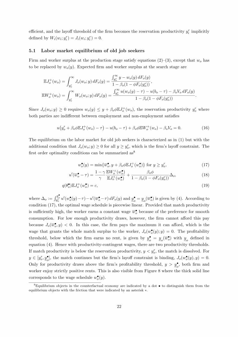
worker enjoy strictly positive rents. This is also visible from Figure 8 where the thick solid line
corresponds to the wage schedule w•o(y).
8Equilibrium objects in the counterfactual economy are indicated by a dot • to distinguish them from theequilibrium objects with the friction that were indicated by an asterisk ∗.
22
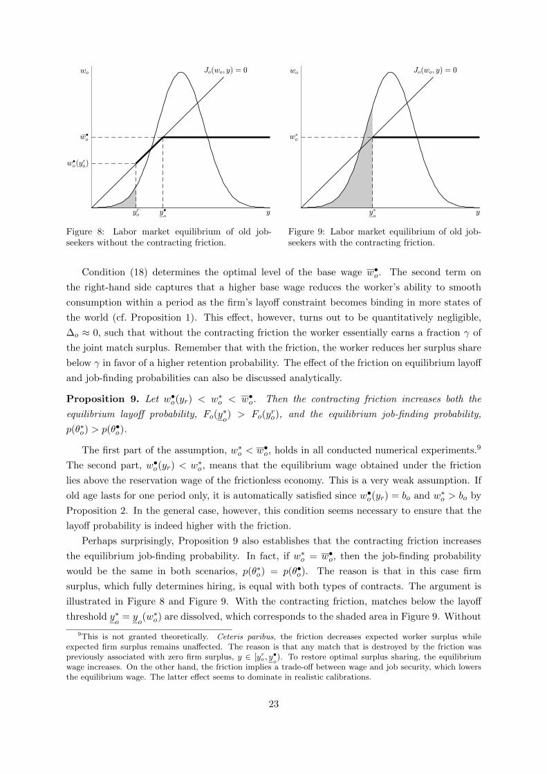
Figure 8: Labor market equilibrium of old job-seekers without the contracting friction.
Figure 9: Labor market equilibrium of old job-seekers with the contracting friction.
Condition (18) determines the optimal level of the base wage w•o. The second term on
the right-hand side captures that a higher base wage reduces the worker’s ability to smooth
consumption within a period as the firm’s layoff constraint becomes binding in more states of
the world (cf. Proposition 1). This effect, however, turns out to be quantitatively negligible,
∆o ≈ 0, such that without the contracting friction the worker essentially earns a fraction γ of
the joint match surplus. Remember that with the friction, the worker reduces her surplus share
below γ in favor of a higher retention probability. The effect of the friction on equilibrium layoff
and job-finding probabilities can also be discussed analytically.
Proposition 9. Let w•o(yr) < w∗o < w•o. Then the contracting friction increases both the
equilibrium layoff probability, Fo(y∗o) > Fo(y
ro), and the equilibrium job-finding probability,
p(θ∗o) > p(θ•o).
The first part of the assumption, w∗o < w•o, holds in all conducted numerical experiments.9
The second part, w•o(yr) < w∗o , means that the equilibrium wage obtained under the friction
lies above the reservation wage of the frictionless economy. This is a very weak assumption. If
old age lasts for one period only, it is automatically satisfied since w•o(yr) = bo and w∗o > bo by
Proposition 2. In the general case, however, this condition seems necessary to ensure that the
layoff probability is indeed higher with the friction.
Perhaps surprisingly, Proposition 9 also establishes that the contracting friction increases
the equilibrium job-finding probability. In fact, if w∗o = w•o, then the job-finding probability
would be the same in both scenarios, p(θ∗o) = p(θ•o). The reason is that in this case firm
surplus, which fully determines hiring, is equal with both types of contracts. The argument is
illustrated in Figure 8 and Figure 9. With the contracting friction, matches below the layoff
threshold y∗o
= yo(w∗o) are dissolved, which corresponds to the shaded area in Figure 9. Without
9This is not granted theoretically. Ceteris paribus, the friction decreases expected worker surplus whileexpected firm surplus remains unaffected. The reason is that any match that is destroyed by the friction waspreviously associated with zero firm surplus, y ∈ [yro , y
•o). To restore optimal surplus sharing, the equilibrium
wage increases. On the other hand, the friction implies a trade-off between wage and job security, which lowersthe equilibrium wage. The latter effect seems to dominate in realistic calibrations.
23
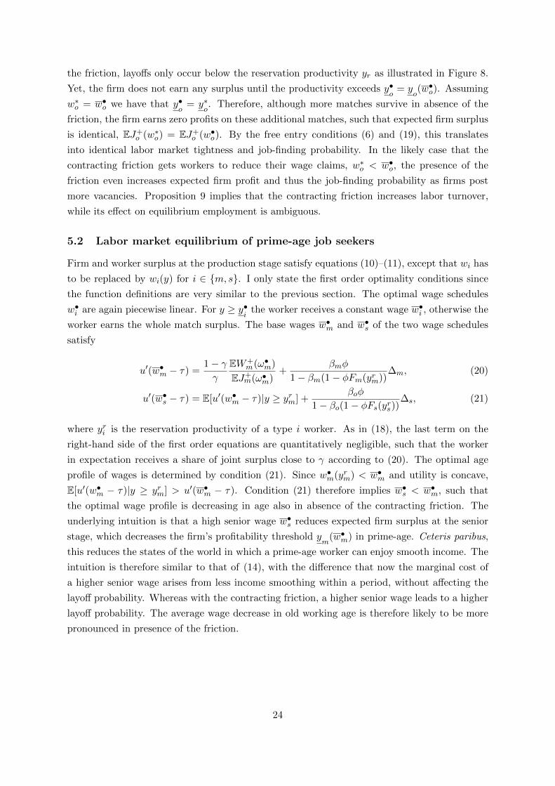
the friction, layoffs only occur below the reservation productivity yr as illustrated in Figure 8.
Yet, the firm does not earn any surplus until the productivity exceeds y•o
= yo(w•o). Assuming
w∗o = w•o we have that y•o
= y∗o. Therefore, although more matches survive in absence of the
friction, the firm earns zero profits on these additional matches, such that expected firm surplus
is identical, EJ+o (w∗o) = EJ+
o (w•o). By the free entry conditions (6) and (19), this translates
into identical labor market tightness and job-finding probability. In the likely case that the
contracting friction gets workers to reduce their wage claims, w∗o < w•o, the presence of the
friction even increases expected firm profit and thus the job-finding probability as firms post
more vacancies. Proposition 9 implies that the contracting friction increases labor turnover,
while its effect on equilibrium employment is ambiguous.
5.2 Labor market equilibrium of prime-age job seekers
Firm and worker surplus at the production stage satisfy equations (10)–(11), except that wi has
to be replaced by wi(y) for i ∈ {m, s}. I only state the first order optimality conditions since
the function definitions are very similar to the previous section. The optimal wage schedules
w•i are again piecewise linear. For y ≥ y•i
the worker receives a constant wage w•i , otherwise the
worker earns the whole match surplus. The base wages w•m and w•s of the two wage schedules
satisfy
u′(w•m − τ) =1− γγ
EW+m(ω•m)
EJ+m(ω•m)
+βmφ
1− βm(1− φFm(yrm))∆m, (20)
u′(w•s − τ) = E[u′(w•m − τ)|y ≥ yrm] +βoφ
1− βo(1− φFs(yrs))∆s, (21)
where yri is the reservation productivity of a type i worker. As in (18), the last term on the
right-hand side of the first order equations are quantitatively negligible, such that the worker
in expectation receives a share of joint surplus close to γ according to (20). The optimal age
profile of wages is determined by condition (21). Since w•m(yrm) < w•m and utility is concave,
E[u′(w•m − τ)|y ≥ yrm] > u′(w•m − τ). Condition (21) therefore implies w•s < w•m, such that
the optimal wage profile is decreasing in age also in absence of the contracting friction. The
underlying intuition is that a high senior wage w•s reduces expected firm surplus at the senior
stage, which decreases the firm’s profitability threshold ym
(w•m) in prime-age. Ceteris paribus,
this reduces the states of the world in which a prime-age worker can enjoy smooth income. The
intuition is therefore similar to that of (14), with the difference that now the marginal cost of
a higher senior wage arises from less income smoothing within a period, without affecting the
layoff probability. Whereas with the contracting friction, a higher senior wage leads to a higher
layoff probability. The average wage decrease in old working age is therefore likely to be more
pronounced in presence of the friction.
24
5.3 Economic aggregates
With productivity-contingent contracts, all demographic and aggregate economic variables are
defined as in Section 4.3, replacing θ∗i with θ•i and y∗i
with yri for i ∈ {m, s, o}. Aggregate welfare
becomes
W1 = EmWm + (N1 − Em)u(bm − τ),
W2 = EsWs + EoWo + (N2 − Eo − Es)u(bo − τ),
where W i =
∫∞yriu(w•i (y)−τ) dFi(y)
1−Fi(yri ) is the average period utility of a type i worker.
6 Numerical illustration and policy implications
To assess the quantitative importance of the contracting friction, I solve the model outlined
in Section 4 numerically and compare it to the counterfactual economy without the friction
described in Section 5. Additionally, I investigate how the presence of the friction affects the
effectiveness of an early retirement reform. Finally, I compare several labor market policies and
discuss their potential to reduce the aggregate costs caused by the contracting friction.
6.1 Calibration
A model period corresponds to a year. The future is discounted at an annual discount rate of
3%, which implies β = 1/1.03 = 0.971. Prime working age lasts from age 25 to 54, while old
working age lasts from age 55 to 64. Therefore, the aging probabilities are set to πm = 1/30 and
πo = 1/10. Productivity follows a normal distribution with mean µi and standard deviation
si. In the baseline, αi = 1 for all worker types, such that the distributions are symmetric. The
mean is normalized to µm = µs = 1 for prime-age and senior workers. For workers hired during
old age, I assume a lower mean productivity of µo = 0.9. This captures that learning and the
adaption to new work requirements becomes more difficult with age, while workers can maintain
high productivity in tasks that they are experienced in (Skirbekk, 2004, 2008). The standard
deviations si are chosen such that for every worker type, productivity in the 90th percentile is
twice as high as in the 10th percentile, which implies sm = ss = 0.2601 and so = 0.2341. As in
Menzio et al. (2016) a productivity draw lasts for 8.5 years on average, such that φ = 0.1167.10
Instantaneous utility exhibits constant absolute risk version, u(w) = (1 − e−κw)/κ. This
specification simplifies the analysis because it eliminates wealth effects. Additionally, it renders
the labor market equilibria independent of the lump sum tax level. I set κ = 3, which in
equilibrium implies rates of relative risk aversion between 2 and 3. The matching function is
Cobb-Douglas m(u, v) = Auγv1−γ with elasticity γ = 0.5 (Petrongolo and Pissarides, 2001).
10Menzio et al. (2016) report a percentile ratio of three, but assume that information is perfect. Mas andMoretti (2009) report a ratio of 0.3 for supermarket cashiers, who perform a very standardized task. I choose anintermediate value that seems consistent with the data.
25
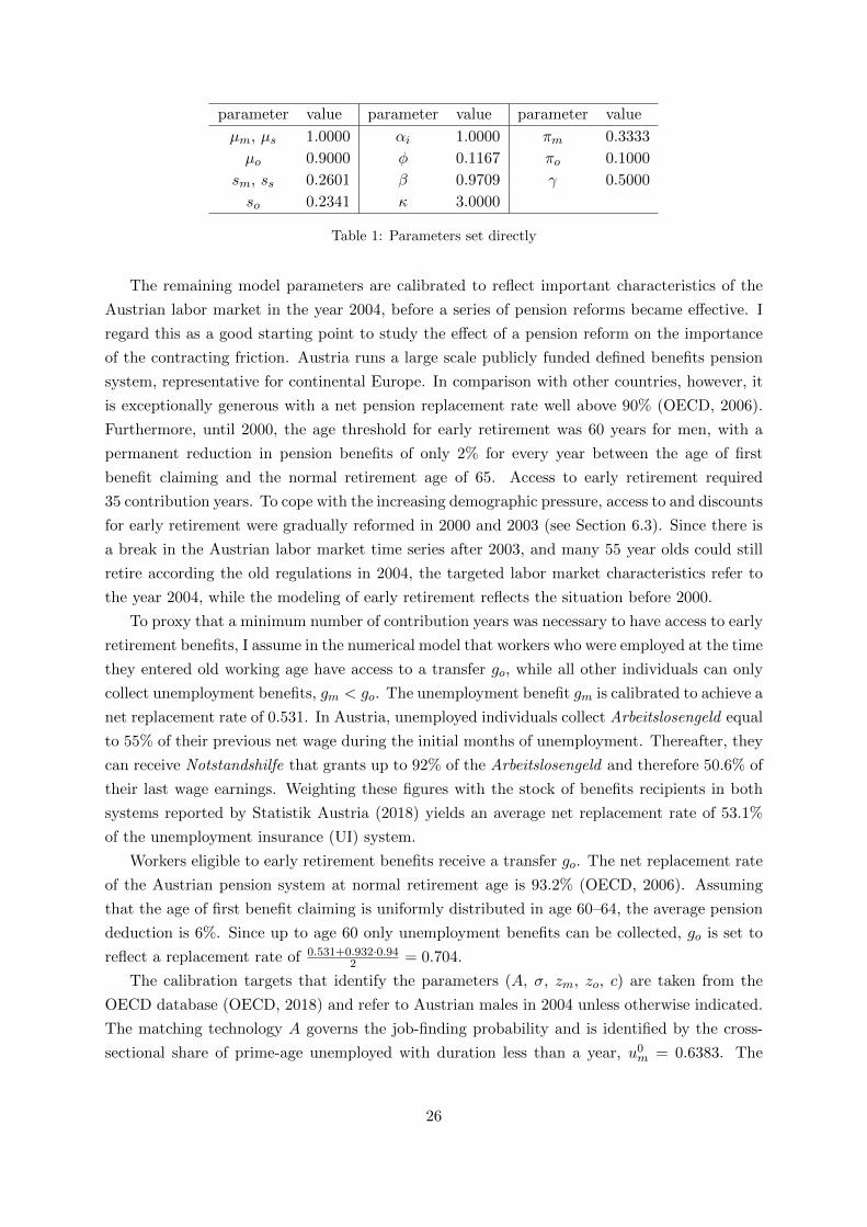
parameter value parameter value parameter value
µm, µs 1.0000 αi 1.0000 πm 0.3333
µo 0.9000 φ 0.1167 πo 0.1000
sm, ss 0.2601 β 0.9709 γ 0.5000
so 0.2341 κ 3.0000
Table 1: Parameters set directly
The remaining model parameters are calibrated to reflect important characteristics of the
Austrian labor market in the year 2004, before a series of pension reforms became effective. I
regard this as a good starting point to study the effect of a pension reform on the importance
of the contracting friction. Austria runs a large scale publicly funded defined benefits pension
system, representative for continental Europe. In comparison with other countries, however, it
is exceptionally generous with a net pension replacement rate well above 90% (OECD, 2006).
Furthermore, until 2000, the age threshold for early retirement was 60 years for men, with a
permanent reduction in pension benefits of only 2% for every year between the age of first
benefit claiming and the normal retirement age of 65. Access to early retirement required
35 contribution years. To cope with the increasing demographic pressure, access to and discounts
for early retirement were gradually reformed in 2000 and 2003 (see Section 6.3). Since there is
a break in the Austrian labor market time series after 2003, and many 55 year olds could still
retire according the old regulations in 2004, the targeted labor market characteristics refer to
the year 2004, while the modeling of early retirement reflects the situation before 2000.
To proxy that a minimum number of contribution years was necessary to have access to early
retirement benefits, I assume in the numerical model that workers who were employed at the time
they entered old working age have access to a transfer go, while all other individuals can only
collect unemployment benefits, gm < go. The unemployment benefit gm is calibrated to achieve a
net replacement rate of 0.531. In Austria, unemployed individuals collect Arbeitslosengeld equal
to 55% of their previous net wage during the initial months of unemployment. Thereafter, they
can receive Notstandshilfe that grants up to 92% of the Arbeitslosengeld and therefore 50.6% of
their last wage earnings. Weighting these figures with the stock of benefits recipients in both
systems reported by Statistik Austria (2018) yields an average net replacement rate of 53.1%
of the unemployment insurance (UI) system.
Workers eligible to early retirement benefits receive a transfer go. The net replacement rate
of the Austrian pension system at normal retirement age is 93.2% (OECD, 2006). Assuming
that the age of first benefit claiming is uniformly distributed in age 60–64, the average pension
deduction is 6%. Since up to age 60 only unemployment benefits can be collected, go is set to
reflect a replacement rate of 0.531+0.932·0.942 = 0.704.
The calibration targets that identify the parameters (A, σ, zm, zo, c) are taken from the
OECD database (OECD, 2018) and refer to Austrian males in 2004 unless otherwise indicated.
The matching technology A governs the job-finding probability and is identified by the cross-
sectional share of prime-age unemployed with duration less than a year, u0m = 0.6383. The
26
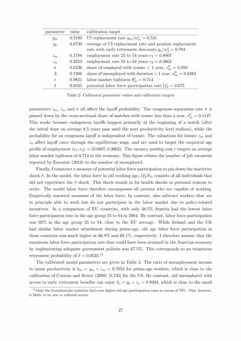
parameter value calibration target
gm 0.5180 UI replacement rate gm/w∗m = 0.531
go 0.6730 average of UI replacement rate and pension replacementrate with early retirement discounts go/w
∗2 = 0.704
zm 0.1788 employment rate 25 to 54 years e1 = 0.8807
zo 0.2553 employment rate 55 to 64 years e2 = 0.3662
σ 0.0236 share of employed with tenure < 1 year, e0m = 0.093
A 0.7406 share of unemployed with duration < 1 year, u0m = 0.6383
c 0.9821 labor market tightness θ∗m = 0.714
δ 0.0535 potential labor force participation rate lf2 = 0.675
Table 2: Calibrated parameter values and calibration targets
parameters zm, zo, and σ all affect the layoff probability. The exogenous separation rate σ is
pinned down by the cross-sectional share of matches with tenure less than a year, e0m = 0.1127.
This works because endogenous layoffs happen primarily at the beginning of a match (after
the initial draw on average 8.5 years pass until the next productivity level realizes), while the
probability for an exogenous layoff is independent of tenure. The valuations for leisure zm and
zo affect layoff rates through the equilibrium wage, and are used to target the empirical age
profile of employment (e1, e2) = (0.8807, 0.3662). The vacancy posting cost c targets an average
labor market tightness of 0.714 in the economy. This figure relates the number of job vacancies
reported by Eurostat (2018) to the number of unemployed.
Finally, I construct a measure of potential labor force participation to pin down the inactivity
shock δ. In the model, the labor force in old working age, lf2N2, consists of all individuals that
did not experience the δ shock. This shock stands in for health shocks or personal reasons to
retire. The model labor force therefore encompasses all persons who are capable of working.
Empirically reported measures of the labor force, by contrast, also subtract workers that are
in principle able to work but do not participate in the labor market due to policy-related
incentives. In a comparison of EU countries, with only 38.5% Austria had the lowest labor
force participation rate in the age group 55 to 64 in 2004. By contrast, labor force participation
was 92% in the age group 25 to 54, close to the EU average. While Ireland and the UK
had similar labor market attachment during prime-age, old age labor force participation in
these countries was much higher at 66.8% and 68.1%, respectively. I therefore assume that the
maximum labor force participation rate that could have been attained in the Austrian economy
by implementing adequate government policies was 67.5%. This corresponds to an exogenous
retirement probability of δ = 0.0535.11
The calibrated model parameters are given in Table 2. The ratio of unemployment income
to mean productivity is bm = gm + zm = 0.7052 for prime-age workers, which is close to the
calibration of Costain and Reiter (2008) [0.745] for the US. By contrast, old unemployed with
access to early retirement benefits can enjoy bo = go + zo = 0.9204, which is close to the small
11Only the Scandinavian countries had even higher old age participation rates in excess of 70%. This, however,is likely to be due to cultural norms.
27
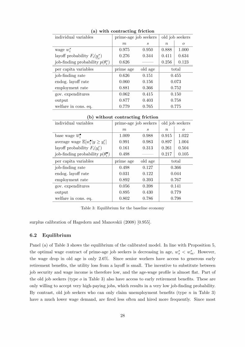
(a) with contracting friction
individual variables prime-age job seekers old job seekers
m s n o
wage w∗i 0.975 0.950 0.888 1.000
layoff probability Fi(y∗i) 0.276 0.344 0.411 0.634
job-finding probability p(θ∗i ) 0.626 ——– 0.256 0.123
per capita variables prime age old age total
job-finding rate 0.626 0.151 0.455
endog. layoff rate 0.060 0.156 0.073
employment rate 0.881 0.366 0.752
gov. expenditures 0.062 0.415 0.150
output 0.877 0.403 0.758
welfare in cons. eq. 0.779 0.765 0.775
(b) without contracting friction
individual variables prime-age job seekers old job seekers
m s n o
base wage w•i 1.009 0.988 0.915 1.022
average wage E[w•i |y ≥ yri ] 0.991 0.983 0.897 1.004
layoff probability Fi(yri ) 0.161 0.313 0.261 0.504
job-finding probability p(θ•i ) 0.498 ——– 0.217 0.105
per capita variables prime age old age total
job-finding rate 0.498 0.127 0.366
endog. layoff rate 0.031 0.122 0.044
employment rate 0.892 0.393 0.767
gov. expenditures 0.056 0.398 0.141
output 0.895 0.430 0.779
welfare in cons. eq. 0.802 0.786 0.798
Table 3: Equilibrium for the baseline economy
surplus calibration of Hagedorn and Manovskii (2008) [0.955].
6.2 Equilibrium
Panel (a) of Table 3 shows the equilibrium of the calibrated model. In line with Proposition 5,
the optimal wage contract of prime-age job seekers is decreasing in age, w∗s < w∗m. However,
the wage drop in old age is only 2.6%. Since senior workers have access to generous early
retirement benefits, the utility loss from a layoff is small. The incentive to substitute between
job security and wage income is therefore low, and the age-wage profile is almost flat. Part of
the old job seekers (type o in Table 3) also have access to early retirement benefits. These are
only willing to accept very high-paying jobs, which results in a very low job-finding probability.
By contrast, old job seekers who can only claim unemployment benefits (type n in Table 3)
have a much lower wage demand, are fired less often and hired more frequently. Since most
28
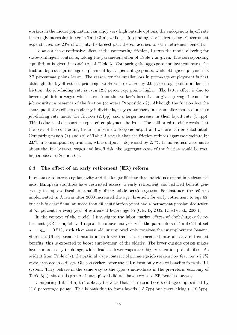
workers in the model population can enjoy very high outside options, the endogenous layoff rate
is strongly increasing in age in Table 3(a), while the job-finding rate is decreasing. Government
expenditures are 20% of output, the largest part thereof accrues to early retirement benefits.
To assess the quantitative effect of the contracting friction, I rerun the model allowing for
state-contingent contracts, taking the parameterization of Table 2 as given. The corresponding
equilibrium is given in panel (b) of Table 3. Comparing the aggregate employment rates, the
friction depresses prime-age employment by 1.1 percentage points, while old age employment is
2.7 percentage points lower. The reason for the smaller loss in prime-age employment is that
although the layoff rate of prime-age workers is elevated by 2.9 percentage points under the
friction, the job-finding rate is even 12.8 percentage points higher. The latter effect is due to
lower equilibrium wages which stem from the worker’s incentive to give up wage income for
job security in presence of the friction (compare Proposition 9). Although the friction has the
same qualitative effects on elderly individuals, they experience a much smaller increase in their
job-finding rate under the friction (2.4pp) and a larger increase in their layoff rate (3.4pp).
This is due to their shorter expected employment horizon. The calibrated model reveals that
the cost of the contracting friction in terms of forgone output and welfare can be substantial.
Comparing panels (a) and (b) of Table 3 reveals that the friction reduces aggregate welfare by
2.9% in consumption equivalents, while output is depressed by 2.7%. If individuals were naive
about the link between wages and layoff risk, the aggregate costs of the friction would be even
higher, see also Section 6.5.
6.3 The effect of an early retirement (ER) reform
In response to increasing longevity and the longer lifetime that individuals spend in retirement,
most European countries have restricted access to early retirement and reduced benefit gen-
erosity to improve fiscal sustainability of the public pension system. For instance, the reforms
implemented in Austria after 2000 increased the age threshold for early retirement to age 62,
but this is conditional on more than 40 contribution years and a permanent pension deduction
of 5.1 percent for every year of retirement before age 65 (OECD, 2005; Knell et al., 2006).
In the context of the model, I investigate the labor market effects of abolishing early re-
tirement (ER) completely. I repeat the above analysis with the parameters of Table 2 but set
go = gm = 0.518, such that every old unemployed only receives the unemployment benefit.
Since the UI replacement rate is much lower than the replacement rate of early retirement
benefits, this is expected to boost employment of the elderly. The lower outside option makes
layoffs more costly in old age, which leads to lower wages and higher retention probabilities. As
evident from Table 4(a), the optimal wage contract of prime-age job seekers now features a 9.7%
wage decrease in old age. Old job seekers after the ER reform only receive benefits from the UI
system. They behave in the same way as the type n individuals in the pre-reform economy of
Table 3(a), since this group of unemployed did not have access to ER benefits anyway.
Comparing Table 4(a) to Table 3(a) reveals that the reform boosts old age employment by
11.8 percentage points. This is both due to fewer layoffs (–5.7pp) and more hiring (+10.5pp).
29
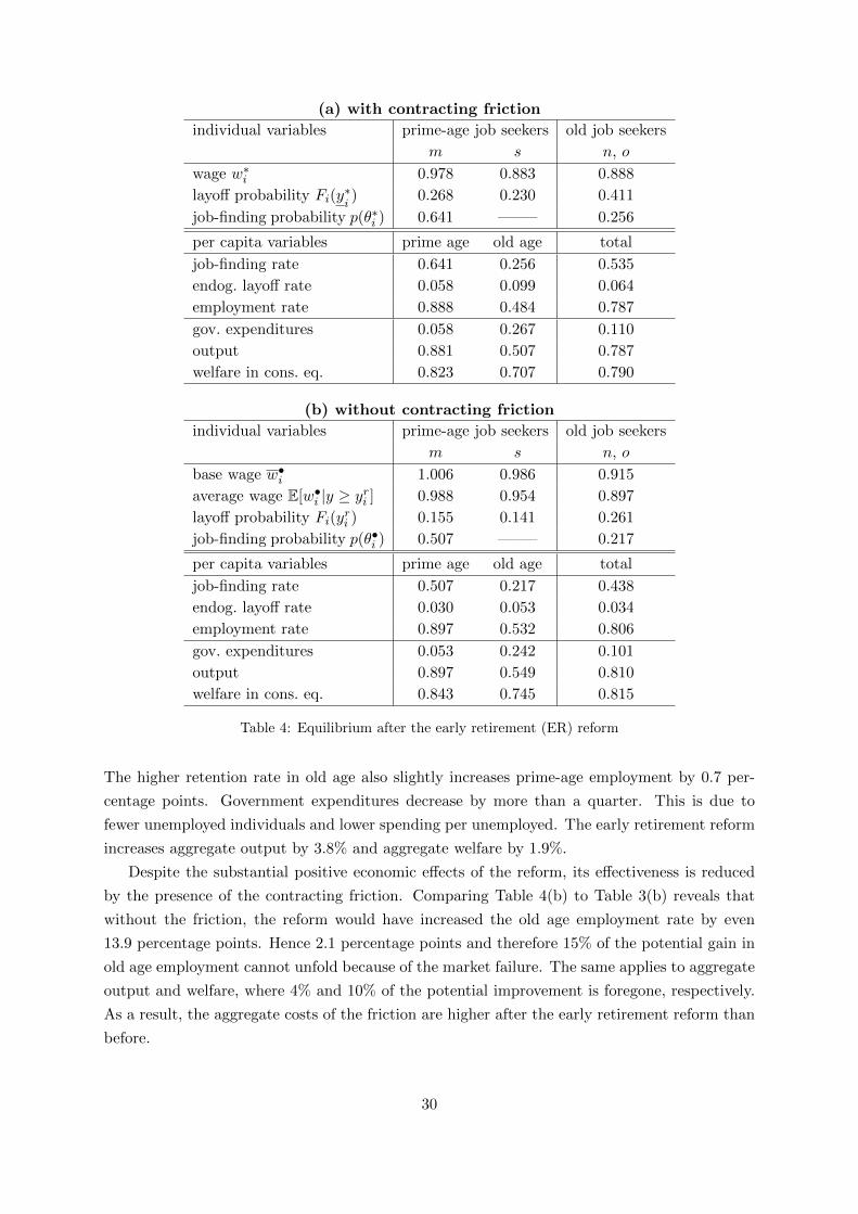
(a) with contracting friction
individual variables prime-age job seekers old job seekers
m s n, o
wage w∗i 0.978 0.883 0.888
layoff probability Fi(y∗i) 0.268 0.230 0.411
job-finding probability p(θ∗i ) 0.641 ——– 0.256
per capita variables prime age old age total
job-finding rate 0.641 0.256 0.535
endog. layoff rate 0.058 0.099 0.064
employment rate 0.888 0.484 0.787
gov. expenditures 0.058 0.267 0.110
output 0.881 0.507 0.787
welfare in cons. eq. 0.823 0.707 0.790
(b) without contracting friction
individual variables prime-age job seekers old job seekers
m s n, o
base wage w•i 1.006 0.986 0.915
average wage E[w•i |y ≥ yri ] 0.988 0.954 0.897
layoff probability Fi(yri ) 0.155 0.141 0.261
job-finding probability p(θ•i ) 0.507 ——– 0.217
per capita variables prime age old age total
job-finding rate 0.507 0.217 0.438
endog. layoff rate 0.030 0.053 0.034
employment rate 0.897 0.532 0.806
gov. expenditures 0.053 0.242 0.101
output 0.897 0.549 0.810
welfare in cons. eq. 0.843 0.745 0.815
Table 4: Equilibrium after the early retirement (ER) reform
The higher retention rate in old age also slightly increases prime-age employment by 0.7 per-
centage points. Government expenditures decrease by more than a quarter. This is due to
fewer unemployed individuals and lower spending per unemployed. The early retirement reform
increases aggregate output by 3.8% and aggregate welfare by 1.9%.
Despite the substantial positive economic effects of the reform, its effectiveness is reduced
by the presence of the contracting friction. Comparing Table 4(b) to Table 3(b) reveals that
without the friction, the reform would have increased the old age employment rate by even
13.9 percentage points. Hence 2.1 percentage points and therefore 15% of the potential gain in
old age employment cannot unfold because of the market failure. The same applies to aggregate
output and welfare, where 4% and 10% of the potential improvement is foregone, respectively.
As a result, the aggregate costs of the friction are higher after the early retirement reform than
before.
30
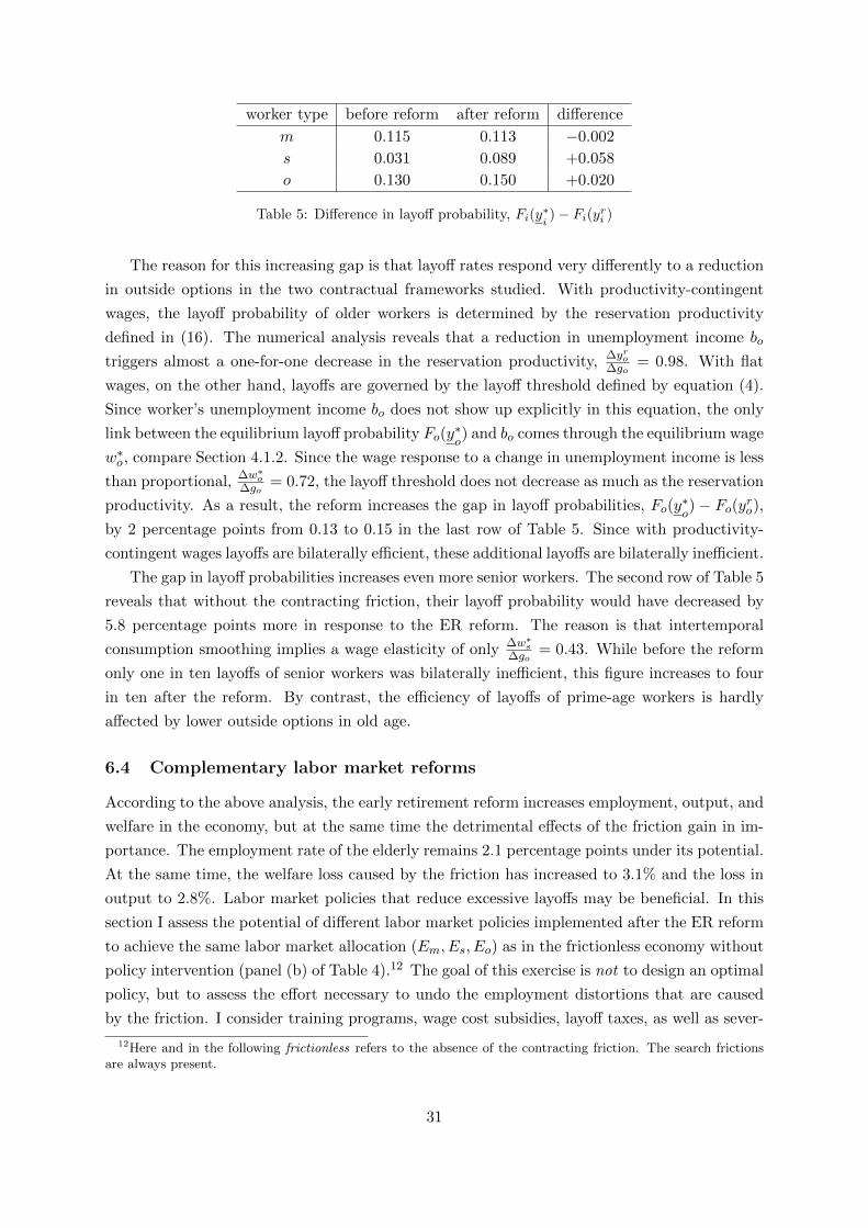
worker type before reform after reform difference
m 0.115 0.113 −0.002
s 0.031 0.089 +0.058
o 0.130 0.150 +0.020
Table 5: Difference in layoff probability, Fi(y∗i)− Fi(y
ri )
The reason for this increasing gap is that layoff rates respond very differently to a reduction
in outside options in the two contractual frameworks studied. With productivity-contingent
wages, the layoff probability of older workers is determined by the reservation productivity
defined in (16). The numerical analysis reveals that a reduction in unemployment income bo
triggers almost a one-for-one decrease in the reservation productivity, ∆yro∆go
= 0.98. With flat
wages, on the other hand, layoffs are governed by the layoff threshold defined by equation (4).
Since worker’s unemployment income bo does not show up explicitly in this equation, the only
link between the equilibrium layoff probability Fo(y∗o) and bo comes through the equilibrium wage
w∗o , compare Section 4.1.2. Since the wage response to a change in unemployment income is less
than proportional, ∆w∗o∆go
= 0.72, the layoff threshold does not decrease as much as the reservation
productivity. As a result, the reform increases the gap in layoff probabilities, Fo(y∗o) − Fo(yro),
by 2 percentage points from 0.13 to 0.15 in the last row of Table 5. Since with productivity-
contingent wages layoffs are bilaterally efficient, these additional layoffs are bilaterally inefficient.
The gap in layoff probabilities increases even more senior workers. The second row of Table 5
reveals that without the contracting friction, their layoff probability would have decreased by
5.8 percentage points more in response to the ER reform. The reason is that intertemporal
consumption smoothing implies a wage elasticity of only ∆w∗s∆go
= 0.43. While before the reform
only one in ten layoffs of senior workers was bilaterally inefficient, this figure increases to four
in ten after the reform. By contrast, the efficiency of layoffs of prime-age workers is hardly
affected by lower outside options in old age.
6.4 Complementary labor market reforms
According to the above analysis, the early retirement reform increases employment, output, and
welfare in the economy, but at the same time the detrimental effects of the friction gain in im-
portance. The employment rate of the elderly remains 2.1 percentage points under its potential.
At the same time, the welfare loss caused by the friction has increased to 3.1% and the loss in
output to 2.8%. Labor market policies that reduce excessive layoffs may be beneficial. In this
section I assess the potential of different labor market policies implemented after the ER reform
to achieve the same labor market allocation (Em, Es, Eo) as in the frictionless economy without
policy intervention (panel (b) of Table 4).12 The goal of this exercise is not to design an optimal
policy, but to assess the effort necessary to undo the employment distortions that are caused
by the friction. I consider training programs, wage cost subsidies, layoff taxes, as well as sever-
12Here and in the following frictionless refers to the absence of the contracting friction. The search frictionsare always present.
31
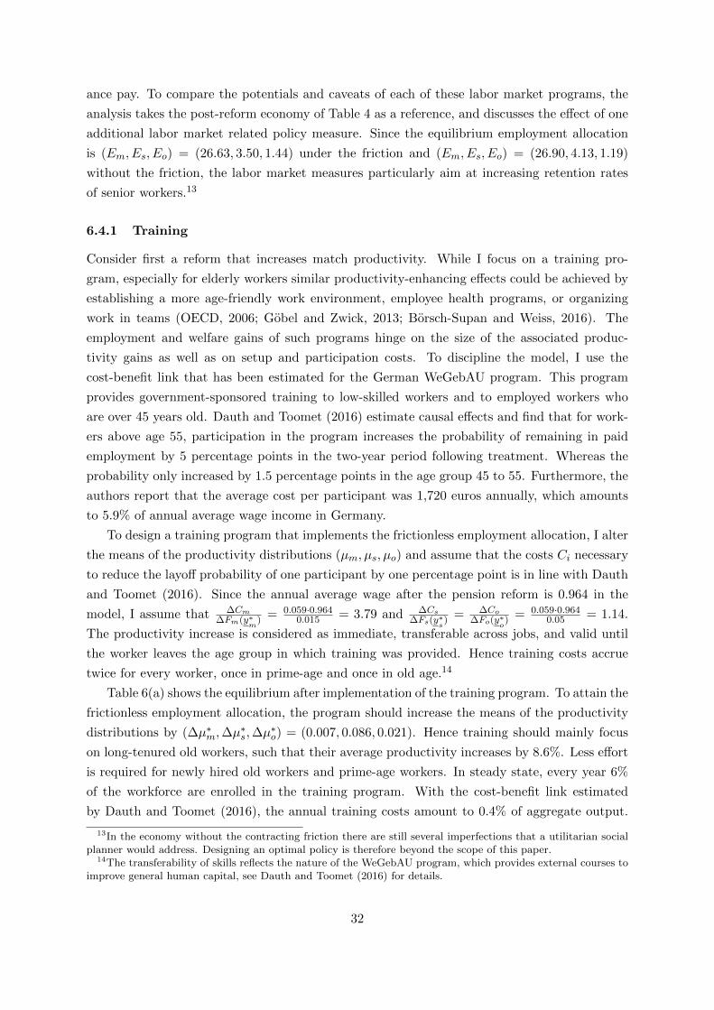
ance pay. To compare the potentials and caveats of each of these labor market programs, the
analysis takes the post-reform economy of Table 4 as a reference, and discusses the effect of one
additional labor market related policy measure. Since the equilibrium employment allocation
is (Em, Es, Eo) = (26.63, 3.50, 1.44) under the friction and (Em, Es, Eo) = (26.90, 4.13, 1.19)
without the friction, the labor market measures particularly aim at increasing retention rates
of senior workers.13
6.4.1 Training
Consider first a reform that increases match productivity. While I focus on a training pro-
gram, especially for elderly workers similar productivity-enhancing effects could be achieved by
establishing a more age-friendly work environment, employee health programs, or organizing
work in teams (OECD, 2006; Gobel and Zwick, 2013; Borsch-Supan and Weiss, 2016). The
employment and welfare gains of such programs hinge on the size of the associated produc-
tivity gains as well as on setup and participation costs. To discipline the model, I use the
cost-benefit link that has been estimated for the German WeGebAU program. This program
provides government-sponsored training to low-skilled workers and to employed workers who
are over 45 years old. Dauth and Toomet (2016) estimate causal effects and find that for work-
ers above age 55, participation in the program increases the probability of remaining in paid
employment by 5 percentage points in the two-year period following treatment. Whereas the
probability only increased by 1.5 percentage points in the age group 45 to 55. Furthermore, the
authors report that the average cost per participant was 1,720 euros annually, which amounts
to 5.9% of annual average wage income in Germany.
To design a training program that implements the frictionless employment allocation, I alter
the means of the productivity distributions (µm, µs, µo) and assume that the costs Ci necessary
to reduce the layoff probability of one participant by one percentage point is in line with Dauth
and Toomet (2016). Since the annual average wage after the pension reform is 0.964 in the
model, I assume that ∆Cm∆Fm(y∗
m) = 0.059·0.964
0.015 = 3.79 and ∆Cs∆Fs(y∗s) = ∆Co
∆Fo(y∗o) = 0.059·0.9640.05 = 1.14.
The productivity increase is considered as immediate, transferable across jobs, and valid until
the worker leaves the age group in which training was provided. Hence training costs accrue
twice for every worker, once in prime-age and once in old age.14
Table 6(a) shows the equilibrium after implementation of the training program. To attain the
frictionless employment allocation, the program should increase the means of the productivity
distributions by (∆µ∗m,∆µ∗s,∆µ
∗o) = (0.007, 0.086, 0.021). Hence training should mainly focus
on long-tenured old workers, such that their average productivity increases by 8.6%. Less effort
is required for newly hired old workers and prime-age workers. In steady state, every year 6%
of the workforce are enrolled in the training program. With the cost-benefit link estimated
by Dauth and Toomet (2016), the annual training costs amount to 0.4% of aggregate output.
13In the economy without the contracting friction there are still several imperfections that a utilitarian socialplanner would address. Designing an optimal policy is therefore beyond the scope of this paper.
14The transferability of skills reflects the nature of the WeGebAU program, which provides external courses toimprove general human capital, see Dauth and Toomet (2016) for details.
32

(a) training program with symmetric returns
individual variables prime-age job seekers old job seekers
m s n, o
wage w∗i 0.988 0.905 0.896
layoff probability Fi(y∗i) 0.256 0.141 0.384
job-finding probability p(θ∗i ) 0.663 ——– 0.276
per capita variables prime age old age total
job-finding rate 0.663 0.276 0.571
endog. layoff rate 0.054 0.067 0.056
employment rate 0.897 0.532 0.806
gov. expenditures 0.055 0.256 0.105
output 0.892 0.586 0.815
welfare in cons. eq. 0.840 0.726 0.807
(b) training program with asymmetric returns
individual variables prime-age job seekers old job seekers
m s n, o
wage w∗i 0.986 0.899 0.893
layoff probability Fi(y∗i) 0.254 0.141 0.379
job-finding probability p(θ∗i ) 0.660 ——– 0.273
per capita variables prime age old age total
job-finding rate 0.660 0.273 0.567
endog. layoff rate 0.054 0.066 0.056
employment rate 0.897 0.532 0.806
gov. expenditures 0.055 0.256 0.106
output 0.892 0.574 0.813
welfare in cons. eq. 0.838 0.724 0.806
Table 6: Equilibrium after the ER reform and implementation of a training program
In total, the program reduces government spending, since the program costs are more than
compensated by lower expenditures on unemployment benefits. Moreover, the welfare cost of
the contracting friction decreases from 3.1% to 1%, while the aggregate output even exceeds
the level of the counterfactual frictionless economy where no policy is implemented.
While this experiment assumed that the productivity of every worker increases uniformly,
it is likely that training has a larger effect on the productivity of low productive workers, and
a smaller effect on workers in the upper tail of the distribution. As evident from Figure 2,
asymmetric returns to training can be captured by an increase in αi, which at the same time
increases the mean and lowers the variance of the distribution. I therefore repeat the above
exercise, but keep µi at their baseline levels and instead alter αi. The frictionless employment
allocation is attained for (∆α∗m,∆α∗s,∆α
∗o) = (0.038, 0.337, 0.105). Table 6(b) shows that while
wages are lower with asymmetric returns, the macroeconomic effects of the two scenarios are
almost identical.
33
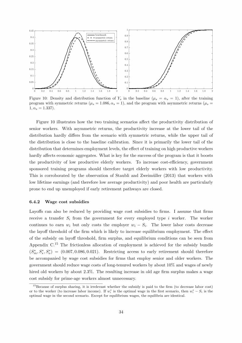
Figure 10: Density and distribution function of Ys in the baseline (µs = αs = 1), after the trainingprogram with symmetric returns (µs = 1.086, αs = 1), and the program with asymmetric returns (µs =1, αs = 1.337).
Figure 10 illustrates how the two training scenarios affect the productivity distribution of
senior workers. With asymmetric returns, the productivity increase at the lower tail of the
distribution hardly differs from the scenario with symmetric returns, while the upper tail of
the distribution is close to the baseline calibration. Since it is primarily the lower tail of the
distribution that determines employment levels, the effect of training on high productive workers
hardly affects economic aggregates. What is key for the success of the program is that it boosts
the productivity of low productive elderly workers. To increase cost-efficiency, government
sponsored training programs should therefore target elderly workers with low productivity.
This is corroborated by the observation of Staubli and Zweimuller (2013) that workers with
low lifetime earnings (and therefore low average productivity) and poor health are particularly
prone to end up unemployed if early retirement pathways are closed.
6.4.2 Wage cost subsidies
Layoffs can also be reduced by providing wage cost subsidies to firms. I assume that firms
receive a transfer Si from the government for every employed type i worker. The worker
continues to earn wi but only costs the employer wi − Si. The lower labor costs decrease
the layoff threshold of the firm which is likely to increase equilibrium employment. The effect
of the subsidy on layoff threshold, firm surplus, and equilibrium conditions can be seen from
Appendix C.15 The frictionless allocation of employment is achieved for the subsidy bundle
(S∗m, S∗s , S
∗o) = (0.007, 0.086, 0.021). Restricting access to early retirement should therefore
be accompanied by wage cost subsidies for firms that employ senior and older workers. The
government should reduce wage costs of long-tenured workers by about 10% and wages of newly
hired old workers by about 2.3%. The resulting increase in old age firm surplus makes a wage
cost subsidy for prime-age workers almost unnecessary.
15Because of surplus sharing, it is irrelevant whether the subsidy is paid to the firm (to decrease labor cost)or to the worker (to increase labor income). If w∗i is the optimal wage in the first scenario, then w∗i − Si is theoptimal wage in the second scenario. Except for equilibrium wages, the equilibria are identical.
34
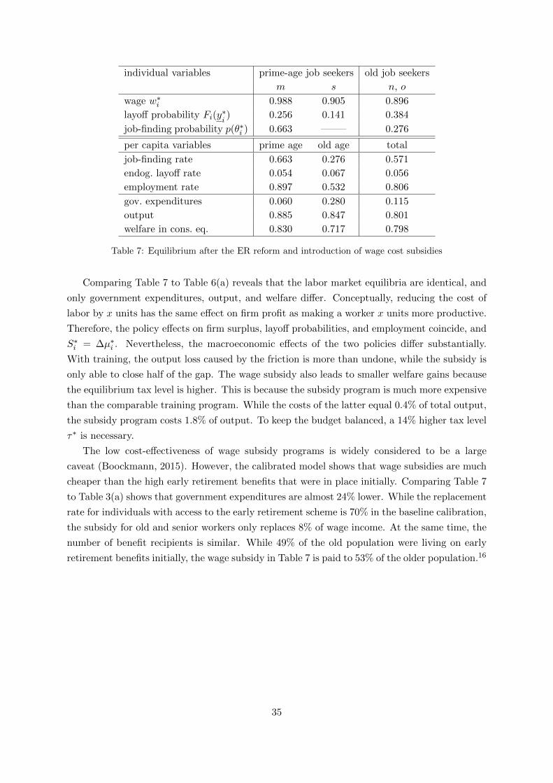
individual variables prime-age job seekers old job seekers
m s n, o
wage w∗i 0.988 0.905 0.896
layoff probability Fi(y∗i) 0.256 0.141 0.384
job-finding probability p(θ∗i ) 0.663 ——– 0.276
per capita variables prime age old age total
job-finding rate 0.663 0.276 0.571
endog. layoff rate 0.054 0.067 0.056
employment rate 0.897 0.532 0.806
gov. expenditures 0.060 0.280 0.115
output 0.885 0.847 0.801
welfare in cons. eq. 0.830 0.717 0.798
Table 7: Equilibrium after the ER reform and introduction of wage cost subsidies
Comparing Table 7 to Table 6(a) reveals that the labor market equilibria are identical, and
only government expenditures, output, and welfare differ. Conceptually, reducing the cost of
labor by x units has the same effect on firm profit as making a worker x units more productive.
Therefore, the policy effects on firm surplus, layoff probabilities, and employment coincide, and
S∗i = ∆µ∗i . Nevertheless, the macroeconomic effects of the two policies differ substantially.
With training, the output loss caused by the friction is more than undone, while the subsidy is
only able to close half of the gap. The wage subsidy also leads to smaller welfare gains because
the equilibrium tax level is higher. This is because the subsidy program is much more expensive
than the comparable training program. While the costs of the latter equal 0.4% of total output,
the subsidy program costs 1.8% of output. To keep the budget balanced, a 14% higher tax level
τ∗ is necessary.
The low cost-effectiveness of wage subsidy programs is widely considered to be a large
caveat (Boockmann, 2015). However, the calibrated model shows that wage subsidies are much
cheaper than the high early retirement benefits that were in place initially. Comparing Table 7
to Table 3(a) shows that government expenditures are almost 24% lower. While the replacement
rate for individuals with access to the early retirement scheme is 70% in the baseline calibration,
the subsidy for old and senior workers only replaces 8% of wage income. At the same time, the
number of benefit recipients is similar. While 49% of the old population were living on early
retirement benefits initially, the wage subsidy in Table 7 is paid to 53% of the older population.16
35
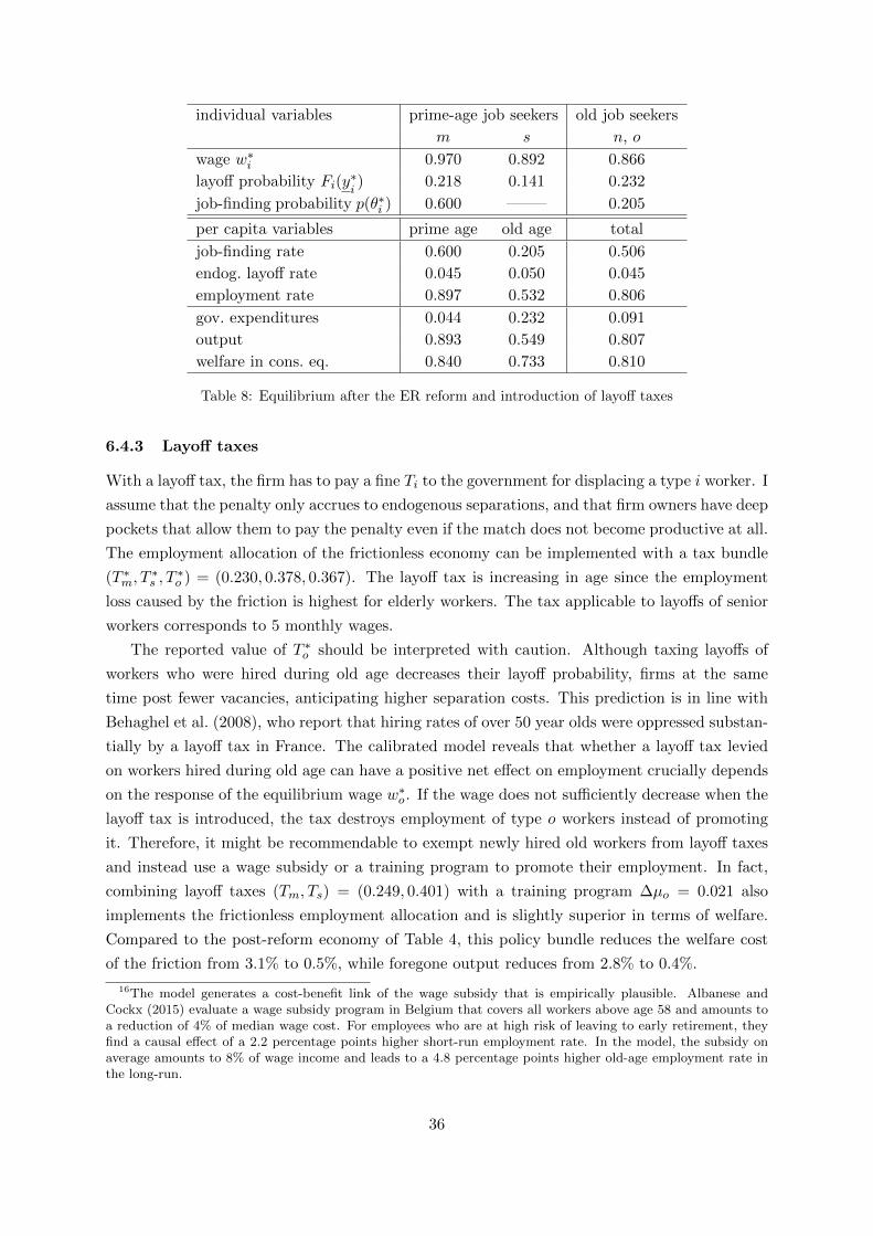
individual variables prime-age job seekers old job seekers
m s n, o
wage w∗i 0.970 0.892 0.866
layoff probability Fi(y∗i) 0.218 0.141 0.232
job-finding probability p(θ∗i ) 0.600 ——– 0.205
per capita variables prime age old age total
job-finding rate 0.600 0.205 0.506
endog. layoff rate 0.045 0.050 0.045
employment rate 0.897 0.532 0.806
gov. expenditures 0.044 0.232 0.091
output 0.893 0.549 0.807
welfare in cons. eq. 0.840 0.733 0.810
Table 8: Equilibrium after the ER reform and introduction of layoff taxes
6.4.3 Layoff taxes
With a layoff tax, the firm has to pay a fine Ti to the government for displacing a type i worker. I
assume that the penalty only accrues to endogenous separations, and that firm owners have deep
pockets that allow them to pay the penalty even if the match does not become productive at all.
The employment allocation of the frictionless economy can be implemented with a tax bundle
(T ∗m, T∗s , T
∗o ) = (0.230, 0.378, 0.367). The layoff tax is increasing in age since the employment
loss caused by the friction is highest for elderly workers. The tax applicable to layoffs of senior
workers corresponds to 5 monthly wages.
The reported value of T ∗o should be interpreted with caution. Although taxing layoffs of
workers who were hired during old age decreases their layoff probability, firms at the same
time post fewer vacancies, anticipating higher separation costs. This prediction is in line with
Behaghel et al. (2008), who report that hiring rates of over 50 year olds were oppressed substan-
tially by a layoff tax in France. The calibrated model reveals that whether a layoff tax levied
on workers hired during old age can have a positive net effect on employment crucially depends
on the response of the equilibrium wage w∗o . If the wage does not sufficiently decrease when the
layoff tax is introduced, the tax destroys employment of type o workers instead of promoting
it. Therefore, it might be recommendable to exempt newly hired old workers from layoff taxes
and instead use a wage subsidy or a training program to promote their employment. In fact,
combining layoff taxes (Tm, Ts) = (0.249, 0.401) with a training program ∆µo = 0.021 also
implements the frictionless employment allocation and is slightly superior in terms of welfare.
Compared to the post-reform economy of Table 4, this policy bundle reduces the welfare cost
of the friction from 3.1% to 0.5%, while foregone output reduces from 2.8% to 0.4%.
16The model generates a cost-benefit link of the wage subsidy that is empirically plausible. Albanese andCockx (2015) evaluate a wage subsidy program in Belgium that covers all workers above age 58 and amounts toa reduction of 4% of median wage cost. For employees who are at high risk of leaving to early retirement, theyfind a causal effect of a 2.2 percentage points higher short-run employment rate. In the model, the subsidy onaverage amounts to 8% of wage income and leads to a 4.8 percentage points higher old-age employment rate inthe long-run.
36
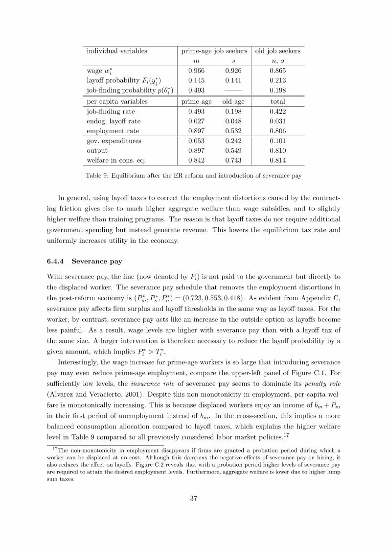
individual variables prime-age job seekers old job seekers
m s n, o
wage w∗i 0.966 0.926 0.865
layoff probability Fi(y∗i) 0.145 0.141 0.213
job-finding probability p(θ∗i ) 0.493 ——– 0.198
per capita variables prime age old age total
job-finding rate 0.493 0.198 0.422
endog. layoff rate 0.027 0.048 0.031
employment rate 0.897 0.532 0.806
gov. expenditures 0.053 0.242 0.101
output 0.897 0.549 0.810
welfare in cons. eq. 0.842 0.743 0.814
Table 9: Equilibrium after the ER reform and introduction of severance pay
In general, using layoff taxes to correct the employment distortions caused by the contract-
ing friction gives rise to much higher aggregate welfare than wage subsidies, and to slightly
higher welfare than training programs. The reason is that layoff taxes do not require additional
government spending but instead generate revenue. This lowers the equilibrium tax rate and
uniformly increases utility in the economy.
6.4.4 Severance pay
With severance pay, the fine (now denoted by Pi) is not paid to the government but directly to
the displaced worker. The severance pay schedule that removes the employment distortions in
the post-reform economy is (P ∗m, P∗s , P
∗o ) = (0.723, 0.553, 0.418). As evident from Appendix C,
severance pay affects firm surplus and layoff thresholds in the same way as layoff taxes. For the
worker, by contrast, severance pay acts like an increase in the outside option as layoffs become
less painful. As a result, wage levels are higher with severance pay than with a layoff tax of
the same size. A larger intervention is therefore necessary to reduce the layoff probability by a
given amount, which implies P ∗i > T ∗i .
Interestingly, the wage increase for prime-age workers is so large that introducing severance
pay may even reduce prime-age employment, compare the upper-left panel of Figure C.1. For
sufficiently low levels, the insurance role of severance pay seems to dominate its penalty role
(Alvarez and Veracierto, 2001). Despite this non-monotonicity in employment, per-capita wel-
fare is monotonically increasing. This is because displaced workers enjoy an income of bm +Pm
in their first period of unemployment instead of bm. In the cross-section, this implies a more
balanced consumption allocation compared to layoff taxes, which explains the higher welfare
level in Table 9 compared to all previously considered labor market policies.17
17The non-monotonicity in employment disappears if firms are granted a probation period during which aworker can be displaced at no cost. Although this dampens the negative effects of severance pay on hiring, italso reduces the effect on layoffs. Figure C.2 reveals that with a probation period higher levels of severance payare required to attain the desired employment levels. Furthermore, aggregate welfare is lower due to higher lumpsum taxes.
37
Boeri et al. (2017) postulate the same contracting friction as this paper and demonstrate
that severance pay can at the same time remove the distortions in the job-finding probability
and in the layoff probability. This neat property does not hold in the present model because
utility is not perfectly transferable between workers and firms due to risk aversion. Comparing
Table 9 to Table 4(b) reveals that while severance pay can restore the equilibrium employment
levels, the labor market is more rigid compared to the frictionless economy due to fewer firing
and fewer hiring. Another implication of risk aversion is that workers always strictly prefer
work over a layoff with severance pay. This is in contrast to Boeri et al. (2017) were workers
are risk neutral and the optimal level of severance pay is such that apart from the first period
of an employment spell, workers are always indifferent between work and being laid off with
severance pay.
As with the layoff tax, the net employment effects of severance pay on old job seekers
crucially depend on the response of equilibrium wages. A combination of severance pay and
training might be a more robust policy and also turns out to be superior in terms of welfare.
The bundle (Pm, Ps,∆µo) = (0.726, 0.558, 0.021) attains the highest welfare level of all labor
market policies considered. The welfare loss relative to the counterfactual economy is only 0.1%.
It should be noted that in practice also other considerations may lead countries to imple-
ment a certain level of severance pay. The important message of the model is that in response
to an early retirement reform, particularly the level of severance pay for long-tenured old work-
ers should be increased. Before the reform, a bundle (Pm, Ps,∆µo) = (0.725, 0.155, 0.020) can
remove the employment distortions of the friction. The early retirement reform therefore par-
ticularly increases the intervention that is necessary to prevent excess layoffs of senior workers.
6.5 Bounded rationality
In Tables 3 and 4 the labor market equilibrium is compared to the equilibrium of the counter-
factual economy without the contracting friction. Ceteris paribus, the presence of the friction
leads to suboptimal employment rates, but this is dampened by lower equilibrium wages. If
workers recognize that lower wages can increase their retention probability, they are willing to
substitute between the two margins. Panel (a) of Table 4 shows that especially senior work-
ers are willing to reduce their wage after the pension reform, such that wages of long-tenured
workers reduce by 10% in the last ten years before retirement. Results from the Structure of
Earnings Survey indicate that the wage-tenure profile of males in Austria have indeed flattened
after 2002. In 2002, the average hourly wage at 20–29 years tenure was 12.3% higher than at
10-19 years tenure. By 2014, this differential has declined to 7.3%, see Figure C.3. Figure C.4
shows that also the cross-sectional age-wage distribution became flatter after age 45. It will be
interesting to see whether these trends continue in future waves of the study.
Nevertheless, it might be questionable whether prime-age job seekers in reality behave as
farsighted as assumed in the model. While they might anticipate that contracting a high wage
today has adverse effects on their retention probability in the near future, it seems much more
difficult to understand how the specificities of the wage contract will affect their chances to
38
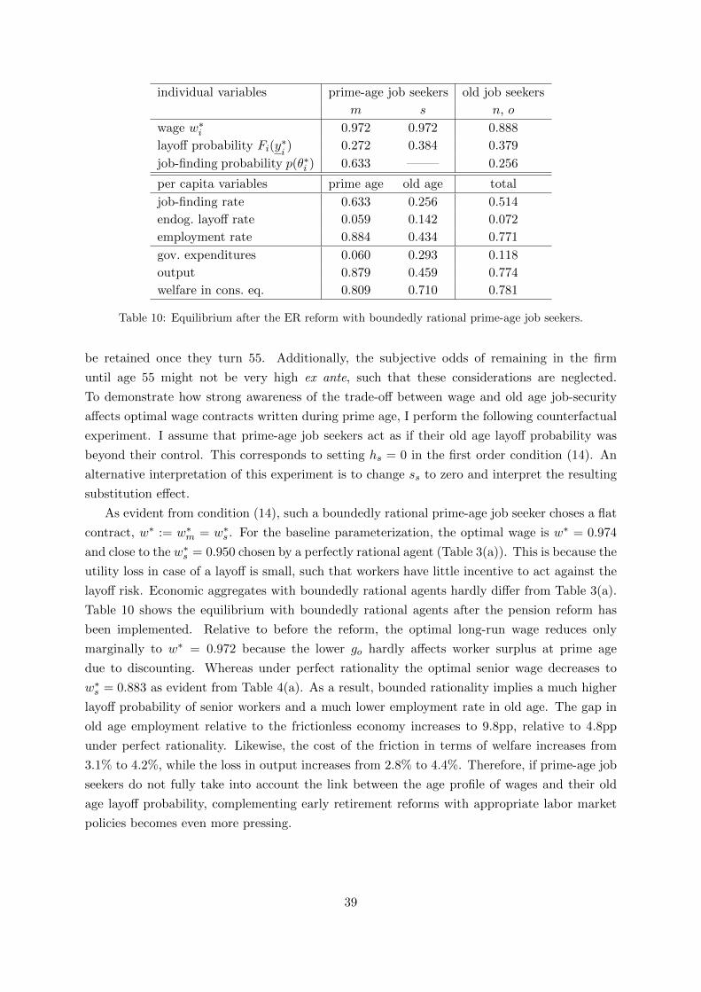
individual variables prime-age job seekers old job seekers
m s n, o
wage w∗i 0.972 0.972 0.888
layoff probability Fi(y∗i) 0.272 0.384 0.379
job-finding probability p(θ∗i ) 0.633 ——– 0.256
per capita variables prime age old age total
job-finding rate 0.633 0.256 0.514
endog. layoff rate 0.059 0.142 0.072
employment rate 0.884 0.434 0.771
gov. expenditures 0.060 0.293 0.118
output 0.879 0.459 0.774
welfare in cons. eq. 0.809 0.710 0.781
Table 10: Equilibrium after the ER reform with boundedly rational prime-age job seekers.
be retained once they turn 55. Additionally, the subjective odds of remaining in the firm
until age 55 might not be very high ex ante, such that these considerations are neglected.
To demonstrate how strong awareness of the trade-off between wage and old age job-security
affects optimal wage contracts written during prime age, I perform the following counterfactual
experiment. I assume that prime-age job seekers act as if their old age layoff probability was
beyond their control. This corresponds to setting hs = 0 in the first order condition (14). An
alternative interpretation of this experiment is to change ss to zero and interpret the resulting
substitution effect.
As evident from condition (14), such a boundedly rational prime-age job seeker choses a flat
contract, w∗ := w∗m = w∗s . For the baseline parameterization, the optimal wage is w∗ = 0.974
and close to the w∗s = 0.950 chosen by a perfectly rational agent (Table 3(a)). This is because the
utility loss in case of a layoff is small, such that workers have little incentive to act against the
layoff risk. Economic aggregates with boundedly rational agents hardly differ from Table 3(a).
Table 10 shows the equilibrium with boundedly rational agents after the pension reform has
been implemented. Relative to before the reform, the optimal long-run wage reduces only
marginally to w∗ = 0.972 because the lower go hardly affects worker surplus at prime age
due to discounting. Whereas under perfect rationality the optimal senior wage decreases to
w∗s = 0.883 as evident from Table 4(a). As a result, bounded rationality implies a much higher
layoff probability of senior workers and a much lower employment rate in old age. The gap in
old age employment relative to the frictionless economy increases to 9.8pp, relative to 4.8pp
under perfect rationality. Likewise, the cost of the friction in terms of welfare increases from
3.1% to 4.2%, while the loss in output increases from 2.8% to 4.4%. Therefore, if prime-age job
seekers do not fully take into account the link between the age profile of wages and their old
age layoff probability, complementing early retirement reforms with appropriate labor market
policies becomes even more pressing.
39
7 Conclusion
In this paper, I have analyzed an age-structured model of the labor market, where wage contracts
are subject to a friction. Contracted wages can depend on age but not on productivity. If realized
productivity is too low, honoring the ex ante optimal wage contract is not profitable for the
firm and a layoff occurs. Since equilibrium wages in general exceed reservation wages, part of
these layoffs are bilaterally inefficient.
The first key insight of the model is that the friction lowers equilibrium wages, and thereby
generates an additional rent for the employer. This leads to more vacancy posting, which partly
counteracts the higher layoff rates. In the calibrated model, the two forces almost offset each
other for prime-age workers, such that the contracting friction only slightly decreases prime-age
employment. This is not the case for elderly workers. Elderly workers in long lasting matches
unequivocally suffer from the higher job destruction rate, while for old job seekers, the increase
in job creation is too small to compensate them for the higher job destruction. Therefore, the
contracting friction particularly depresses employment rates in old working age.
The second key insight of the model is that the contracting friction dampens the positive
economic effects of reforms to the early retirement system. In the numerical analysis, about
15% of the potential gain in old age employment cannot be realized because of the friction.
The reason is that with the friction, the layoff probability reacts less sensibly to changes in
the worker’s outside option. As a result, pushing back a government failure (granting excessive
outside options to the elderly) increases the detrimental effects of the market failure. Reforms
that make early retirement less attractive should therefore be accompanied by labor market
policies that increase firms’ willingness to keep elderly workers employed. The quantitative
results suggest that increasing employment protection for long-tenured old workers is most
effective in this regard. The urgency of labor market reforms increases if prime-age job seekers
do not take into account that the age profile of wages affects their job security in late working
age.
40
References
D. Acemoglu and R. Shimer. Efficient Unemployment Insurance. Journal of Political Economy,107(5):893–928, 1999.
A. Albanese and B. Cockx. Permanent Wage Cost Subsidies for Older Workers: An EffectiveTool for Increasing Working Time and Postponing Early Retirement? IZA Discussion PaperNo. 8988, 2015.
F. Alvarez and M. Veracierto. Severance payments in an economy with frictions. Journal ofMonetary Economics, 47(3):477–498, 2001.
L. Behaghel, B. Crepon, and B. Sedillot. The perverse effects of partial employment protectionreform: The case of French older workers. Journal of Public Economics, 92(3-4):696–721,2008.
T. Boeri, P. Garibaldi, and E. R. Moen. Inside severance pay. Journal of Public Economics,145:211–225, 2017.
B. Boockmann. The effects of wage subsidies for older workers. IZA World of Labor, 189:1–10,September 2015.
A. Borsch-Supan and M. Weiss. Productivity and age: Evidence from work teams at theassembly line. Journal of the Economics of Ageing, 7:30–42, 2016.
A. Cheron, J.-O. Hairault, and F. Langot. Age-dependent employment protection. The Eco-nomic Journal, 121(557):1477–1504, 2011.
A. Cheron, J.-O. Hairault, and F. Langot. Life-cycle equilibrium unemployment. Journal ofLabor Economics, 31(4):843–882, 2013.
J. S. Costain and M. Reiter. Business cycles, unemployment insurance, and the calibration ofmatching models. Journal of Economic Dynamics and Control, 32(4):1120–1155, 2008.
C. Dauth and O.-S. Toomet. On government-subsidized training programs for older workers.Labour, 30:371–392, 2016.
L. Diez-Catalan and E. Villanueva. Contract staggering and unemployment during the greatrecession: evidence from Spain. Banco de Espana Working Paper No. 1431, 2015.
D. Dorn and A. Sousa-Poza. ’Voluntary’ and ’involuntary’ early retirement: an internationalanalysis. Applied Economics, 42(4):427–438, 2010.
C. Dustmann and U. Schonberg. Training and union wages. The Review of Economics andStatistics, 91(2):363–376, 2009.
Eurostat. Transition from work to retirement – evaluation of the 2012 labour forcesurvey ad hoc module. http://ec.europa.eu/eurostat/documents/1978984/6037334/
Evaluation-Report-AHM-2012.pdf, 2012.
Eurostat. Job vacancy statistics by occupation, NUTS 2 regions and NACE Rev. 1.1 activity -annual data (2000-2008), 2018. URL http://appsso.eurostat.ec.europa.eu/nui/show.
do?dataset=jvs_a_nace1. Date accessed: Feb. 11, 2018.
W. H. Fisher and C. Keuschnigg. Pension reform and labor market incentives. Journal ofPopulation Economics, 23(2):769–803, 2008.
41
W. Frimmel, T. Horvath, M. Schnalzenberger, and R. Winter-Ebmer. Seniority wages and therole of firms in retirement. Journal of Public Economics, 164:19–32, 2018.
C. Gobel and T. Zwick. Are personnel measures effective in increasing productivity of oldworkers? Labour Economics, 22:80–93, 2013.
P. Guimaraes, F. Martins, and P. Portugal. Upward Nominal Wage Rigidity. IZA DiscussionPaper No. 10510, 2017.
M. Hagedorn and I. Manovskii. The Cyclical Behavior of Equilibrium Unemployment andVacancies Revisited. American Economic Review, 98(4):1692–1706, 2008.
J.-O. Hairault, F. Langot, and A. Zylberberg. Equilibrium unemployment and retirement.European Economic Review, 79:37–58, 2015.
R. E. Hall and E. P. Lazear. The excess sensitivity of layoffs and quits to demand. Journal ofLabor Economics, 2(2):233–257, 1984.
M. Hashimoto. Human Capital as a Shared Investment. American Economic Review, 71(3):475–482, 1981.
A. Hornstein, P. Krusell, and G. L. Violante. Unemployment and vacancy fluctuations in thematching model: inspecting the mechanism. Economic Quarterly, 91(3):19–50, 2005.
C. Jaag, C. Keuschnigg, and M. Keuschnigg. Pension reform, retirement, and life-cycle unem-ployment. International Tax and Public Finance, 17(5):556–585, 2010.
J. Kennan. Private Information, Wage Bargaining and Employment Fluctuations. The Reviewof Economic Studies, 77(2):633–664, 2010.
M. Knell, W. Kohler-Toglhofer, and D. Prammer. Jungste Pensionsreformen in Osterreichund ihre Auswirkungen auf fiskalische Nachhaltigkeit und Pensionsleistungen. Geldpolitik &Wirtschaft, Q2:72–100, 2006.
R. Konle-Seidl. Retention and Re-integration of older workers into the labour market: Whatworks? IAB Discussion Paper 17/2017, 2017.
E. P. Lazear. Why is there mandatory retirement? The Journal of Political Economy, 87(6):1261–1284, 1979.
M. Marmot, J. Banks, R. Blundell, C. Lessof, and J. Nazroo. Health, wealth and lifestyles ofthe older population in England: ELSA 2002. Institute for Fiscal Studies, 2003.
A. Mas and E. Moretti. Peers at Work. American Economic Review, 99(1):112–145, 2009.
G. Menzio, I. A. Telyukova, and L. Visschers. Directed search over the life cycle. Review ofEconomic Dynamics, 19:38–62, 2016.
E. R. Moen. Competitive Search Equilibrium. Journal of Political Economy, 105(2):385–411,1997.
D. T. Mortensen and C. A. Pissarides. New developments in models of search in the labormarket. In O. C. Ashenfelter and D. Card, editors, Handbook of Labor Economics, volume 3,part B, chapter 39, pages 2567–2627. Elsevier, 1999.
OECD. Ageing and Employment Policies: Austria. OECD Publishing, 2005.
42
OECD. Live Longer, Work Longer. Ageing and Employment Policies. OECD Publishing, 2006.
OECD. LFS by sex and age, 2018. URL https://stats.oecd.org/Index.aspx?DataSetCode=
LFS_SEXAGE_I_R. Date accessed: Feb. 11, 2018.
B. Petrongolo and C. Pissarides. Looking into the black box: a survey of the matching function.Journal of Economic Literature, 39(2):390–431, 2001.
G. Ramey and J. Watson. Contractual fragility, job destruction, and business cycles. TheQuarterly Journal of Economics, 112(3):873–911, 1997.
M. R. Sampford. Some Inequalities on Mill’s Ratio and Related Functions. The Annals ofMathematical Statistics, 24(1):130–132, 1953.
R. Shimer. Essays in search theory. PhD Thesis, Massachusetts Institute of Technology, 1996.
V. Skirbekk. Age and Individual Productivity: A Literature Survey. Vienna Yearbook ofPopulation Research, 1:133–154, 2004.
V. Skirbekk. Age and productivity capacity: descriptions, causes and policy options. AgeingHorizons, 8:4–12, 2008.
Statistik Austria. Verdienststrukturerhebung 2002. Verlag Osterreich GmbH, 2006.
Statistik Austria. Verdienststrukturerhebung 2006. Verlag Osterreich GmbH, 2009.
Statistik Austria. Verdienststrukturerhebung 2014. Verlag Osterreich GmbH, 2017.
Statistik Austria. Arbeitslosenleistungen, 2018. URL http://statistik.at/web_
de/statistiken/menschen_und_gesellschaft/soziales/sozialleistungen_auf_
bundesebene/arbeitslosenleistungen/index.html. Date accessed: Feb. 11, 2018.
S. Staubli and J. Zweimuller. Does raising the early retirement age increase employment ofolder workers? Journal of Public Economics, 108:17–32, 2013.
A. Weiss. Job Queues and Layoffs in Labor Markets with Flexible Wages. Journal of PoliticalEconomy, 88(3):526–538, 1980.
R. Winter-Ebmer. Benefit duration and unemployment entry: A quasi-experiment in Austria.European Economic Review, 47:259–273, 2003.
43
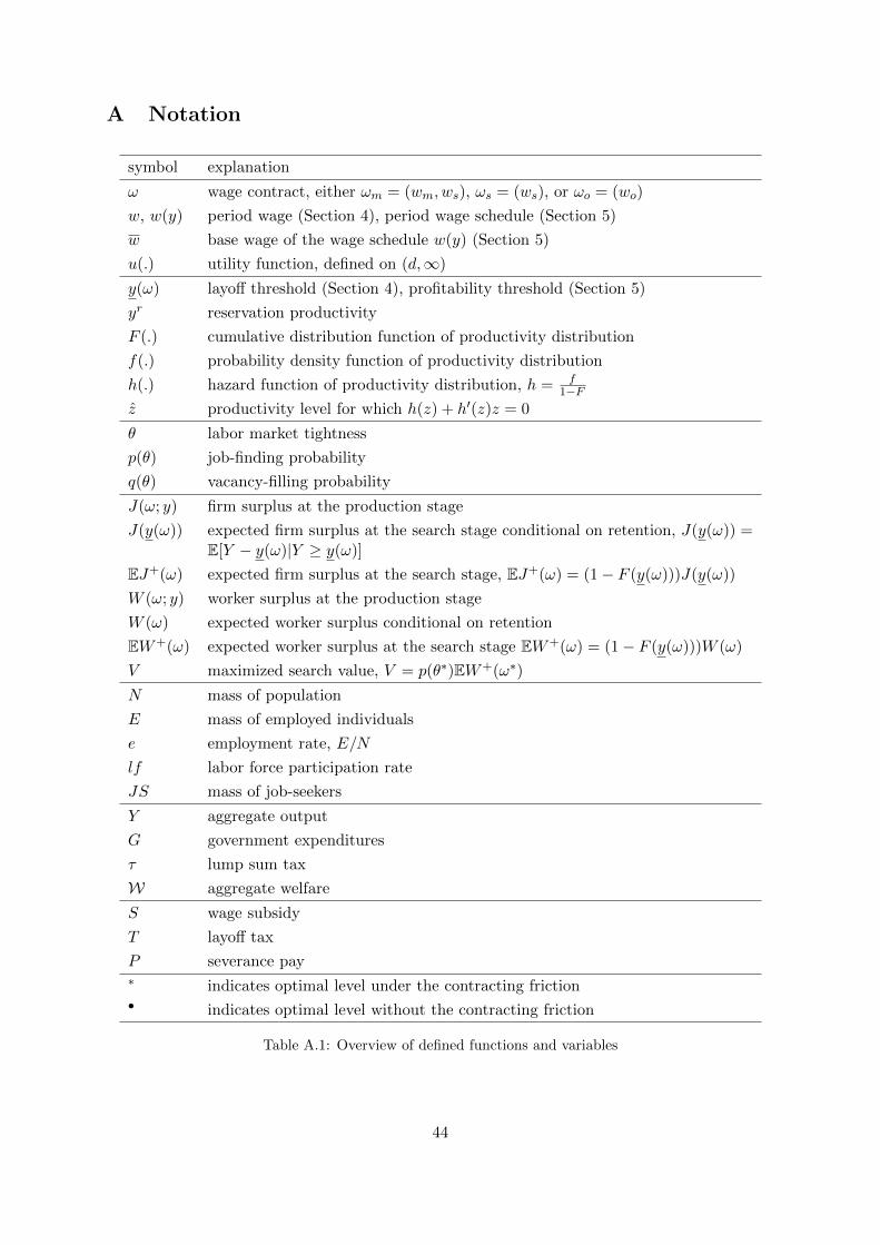
A Notation
symbol explanation
ω wage contract, either ωm = (wm, ws), ωs = (ws), or ωo = (wo)
w, w(y) period wage (Section 4), period wage schedule (Section 5)
w base wage of the wage schedule w(y) (Section 5)
u(.) utility function, defined on (d,∞)
y(ω) layoff threshold (Section 4), profitability threshold (Section 5)
yr reservation productivity
F (.) cumulative distribution function of productivity distribution
f(.) probability density function of productivity distribution
h(.) hazard function of productivity distribution, h = f1−F
z productivity level for which h(z) + h′(z)z = 0
θ labor market tightness
p(θ) job-finding probability
q(θ) vacancy-filling probability
J(ω; y) firm surplus at the production stage
J(y(ω)) expected firm surplus at the search stage conditional on retention, J(y(ω)) =E[Y − y(ω)|Y ≥ y(ω)]
EJ+(ω) expected firm surplus at the search stage, EJ+(ω) = (1− F (y(ω)))J(y(ω))
W (ω; y) worker surplus at the production stage
W (ω) expected worker surplus conditional on retention
EW+(ω) expected worker surplus at the search stage EW+(ω) = (1− F (y(ω)))W (ω)
V maximized search value, V = p(θ∗)EW+(ω∗)
N mass of population
E mass of employed individuals
e employment rate, E/N
lf labor force participation rate
JS mass of job-seekers
Y aggregate output
G government expenditures
τ lump sum tax
W aggregate welfare
S wage subsidy
T layoff tax
P severance pay∗ indicates optimal level under the contracting friction• indicates optimal level without the contracting friction
Table A.1: Overview of defined functions and variables
44

symbol explanation
µi location parameter of the productivity distribution
si scale parameter (dispersion) of the productivity distribution
αi shape parameter of the productivity distribution
φ probability of drawing a new match productivity
κ coefficient of absolute risk aversion
bi unemployment income, bi = gi + zi
gi government transfer to unemployed individuals
zi value of leisure, home production
πm transition probability from prime working age to old working age
πo transition probability from old working age to retirement age
β time discount factor
βi effective discount factor, βm = β(1− πm)(1− σ), βo = β(1− πo)(1− σ)(1− δ)σ probability of an exogenous separation
δ probability of an inactivity shock
A level of matching technology
γ elasticity of the matching function
c period cost of posting a vacancy
Table A.2: Overview of model parameters
B Mathematical appendix
B.1 Properties of the normal and logistic distribution
This section verifies that the hazard functions of the standard normal and the standard logistic
distribution satisfy properties (iii) and (iv) of Assumption 1.
Normal distribution. The pdf of the standard normal distribution is f(z) = 1√2πe−z
2/2, and
the cdf is F (z) = 1√2π
∫ z−∞ e
−t2/2 dt. The hazard function can be written h(z) = e−z2/2[ ∫∞
z e−t2/2 dt
]−1.
The growth rate of the hazard is γh(z) := h′(z)h(z) = h(z) − z, which implies γ′h(z) = h′(z) − 1 =
h(z)[h(z)−z]−1. According to Sampford (1953), the hazard rate satisfies 0 < h(z)[h(z)−z] < 1,
which implies γh(z) > 0 and γ′h(z) < 0 for z ∈ R. Furthermore, convexity of the conditional
expectation follows from E[Z − a|Z ≥ a] = h(a) − a and the fact that the hazard rate of the
normal distribution is strictly convex (Sampford, 1953).
Logistic distribution. The pdf of the standard logistic distribution is f(z) = e−z
(1+e−z)2, and
the cdf is F (z) = 11+e−z . The hazard function is h(z) = 1
1+e−z = F (z). Therefore, γh(z) =
h′(z)/h(z) = f(z)/F (z) = 1 − F (z) > 0, and γ′h(z) = −f(z) < 0. The conditional expectation
E[Z − a|Z ≥ a] = ln(1+e−a)1+ea is strictly convex in a.
The same properties can be established for the Gumbel distribution and the Weibull distri-
bution with shape parameter k > 1. The proofs are available by request from the author.
45

B.2 Additional lemmas
The hazard rate is a central object in the analysis. The following Lemma B.1 summarizes
important properties:
Lemma B.1. Consider the hazard rate hi(y) = fi(y)1−Fi(y) and define the elasticity εh(z) = h′(z)z
h(z) .
Under Assumption 1 and Assumption 3, the partial derivatives satisfy the following properties:
(i) h′i(y) > 0,
(ii) ∂hi(y)∂µi
= −h′i(y),
(iii) ∂hi(y)∂si
Q 0 for y−µisi
R z, where z < 0 is characterized by εh(z) = −1.
Proof. The imposed assumptions imply that the density of Yi is fi(y) = 1sif(z) where z =
y−µisi
. The hazard rate is therefore hi(y) = 1sih(z). Properties (i) and (ii) directly follow from
monotonicity of h. Differentiation of hi with respect to si gives ∂hi(y)∂si
= − 1s2i
[h(z) + h′(z)z].
The sign of ∂hi(y)∂si
is therefore the opposite of k(z) := 1 + εh(z). Since k(0) = 1 and h′ > 0,
any root of k must lie in the negative domain. For z < 0, Assumption 1(iii) implies that
k′(z) = ddz
[h′(z)h(z)
]z + h′(z)
h(z) > 0. Hence there exists a unique z < 0 with k(z) = 0.
Another object that repeatedly occurs in the analysis are conditional expectations of the
form E[Yi − a|Yi ≥ a].
Lemma B.2. Consider the conditional expectation Ji(a) := E[Yi − a|Yi ≥ a] =∫∞a y−a dFi(y)
1−Fi(a) .
Under Assumptions 1 and 3, the following properties hold:
(i) max{0,EYi − a} < Ji(a) < hi(a)−1,
(ii) lima→−∞
[Ji(a) + a
]= EYi,
(iii) lima→∞
[Ji(a)− hi(a)−1
]= 0,
(iv) J ′i(a) < 0, ∂Ji(a)∂µi
= −J ′i(a), ∂Ji(a)∂si
> 0
Proof. Since the integrand in Ji(a) is non-negative, Ji(a) > 0 follows from the definition. The
upper bound can be found using integration by parts and exploiting the monotonicity of the
hazard function,
Ji(a) =
∫∞a 1− Fi(y) dy
1− Fi(a)=
∫∞a fi(y)/hi(y) dy
1− Fi(a)<
∫∞a fi(y) dy
1− Fi(a)
1
hi(a)=
1
hi(a).
This inequality also implies that Ji(a) is monotonically decreasing, J ′i(a) = −1+Ji(a)hi(a) < 0.
The existence of a second lower bound in (i) and the limit in (ii) can be shown together. Define
the auxiliary function l(a) := Ji(a) + a =∫∞a ydFi(y)
1−Fi(a) . Substituting the above expression for the
derivative yields l′(a) = J ′i(a) + 1 = Ji(a)hi(a) > 0. Furthermore, l(a) converges to EYi if a
tends to −∞. Therefore, l(a) > EYi for all a ∈ R, and the bound is approached in the limit.
Property (iii) follows from L’Hospital’s rule, lima→∞ Ji(a) = lima→∞1−Fi(a)fi(a) = lima→∞ hi(a)−1.
46
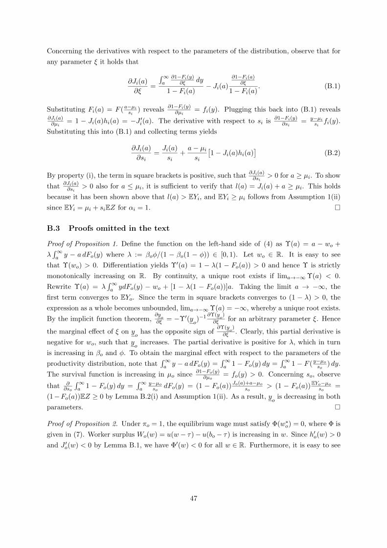
Concerning the derivatives with respect to the parameters of the distribution, observe that for
any parameter ξ it holds that
∂Ji(a)
∂ξ=
∫∞a
∂1−Fi(y)∂ξ dy
1− Fi(a)− Ji(a)
∂1−Fi(a)∂ξ
1− Fi(a). (B.1)
Substituting Fi(a) = F (a−µisi) reveals ∂1−Fi(y)
∂µi= fi(y). Plugging this back into (B.1) reveals
∂Ji(a)∂µi
= 1 − Ji(a)hi(a) = −J ′i(a). The derivative with respect to si is ∂1−Fi(y)∂si
= y−µisi
fi(y).
Substituting this into (B.1) and collecting terms yields
∂Ji(a)
∂si=Ji(a)
si+a− µisi
[1− Ji(a)hi(a)
](B.2)
By property (i), the term in square brackets is positive, such that ∂Ji(a)∂si
> 0 for a ≥ µi. To show
that ∂Ji(a)∂si
> 0 also for a ≤ µi, it is sufficient to verify that l(a) = Ji(a) + a ≥ µi. This holds
because it has been shown above that l(a) > EYi, and EYi ≥ µi follows from Assumption 1(ii)
since EYi = µi + siEZ for αi = 1.
B.3 Proofs omitted in the text
Proof of Proposition 1. Define the function on the left-hand side of (4) as Υ(a) = a − wo +
λ∫∞a y − a dFo(y) where λ := βoφ/(1 − βo(1 − φ)) ∈ [0, 1). Let wo ∈ R. It is easy to see
that Υ(wo) > 0. Differentiation yields Υ′(a) = 1 − λ(1 − Fo(a)) > 0 and hence Υ is strictly
monotonically increasing on R. By continuity, a unique root exists if lima→−∞Υ(a) < 0.
Rewrite Υ(a) = λ∫∞a ydFo(y) − wo + [1 − λ(1 − Fo(a))]a. Taking the limit a → −∞, the
first term converges to EYo. Since the term in square brackets converges to (1 − λ) > 0, the
expression as a whole becomes unbounded, lima→−∞Υ(a) = −∞, whereby a unique root exists.
By the implicit function theorem,∂yo
∂ξ = −Υ′(yo)−1 ∂Υ(y
o)
∂ξ for an arbitrary parameter ξ. Hence
the marginal effect of ξ on yo
has the opposite sign of∂Υ(y
o)
∂ξ . Clearly, this partial derivative is
negative for wo, such that yo
increases. The partial derivative is positive for λ, which in turn
is increasing in βo and φ. To obtain the marginal effect with respect to the parameters of the
productivity distribution, note that∫∞a y − a dFo(y) =
∫∞a 1 − Fo(y) dy =
∫∞a 1 − F (y−µoso
) dy.
The survival function is increasing in µo since ∂1−Fo(y)∂µo
= fo(y) > 0. Concerning so, observe
that ∂∂so
∫∞a 1 − Fo(y) dy =
∫∞a
y−µoso
dFo(y) = (1 − Fo(a))Jo(a)+a−µoso
> (1 − Fo(a))EYo−µoso=
(1−Fo(a))EZ ≥ 0 by Lemma B.2(i) and Assumption 1(ii). As a result, yo
is decreasing in both
parameters.
Proof of Proposition 2. Under πo = 1, the equilibrium wage must satisfy Φ(w∗o) = 0, where Φ is
given in (7). Worker surplus Wo(w) = u(w− τ)− u(bo − τ) is increasing in w. Since h′o(w) > 0
and J ′o(w) < 0 by Lemma B.1, we have Φ′(w) < 0 for all w ∈ R. Furthermore, it is easy to see
47
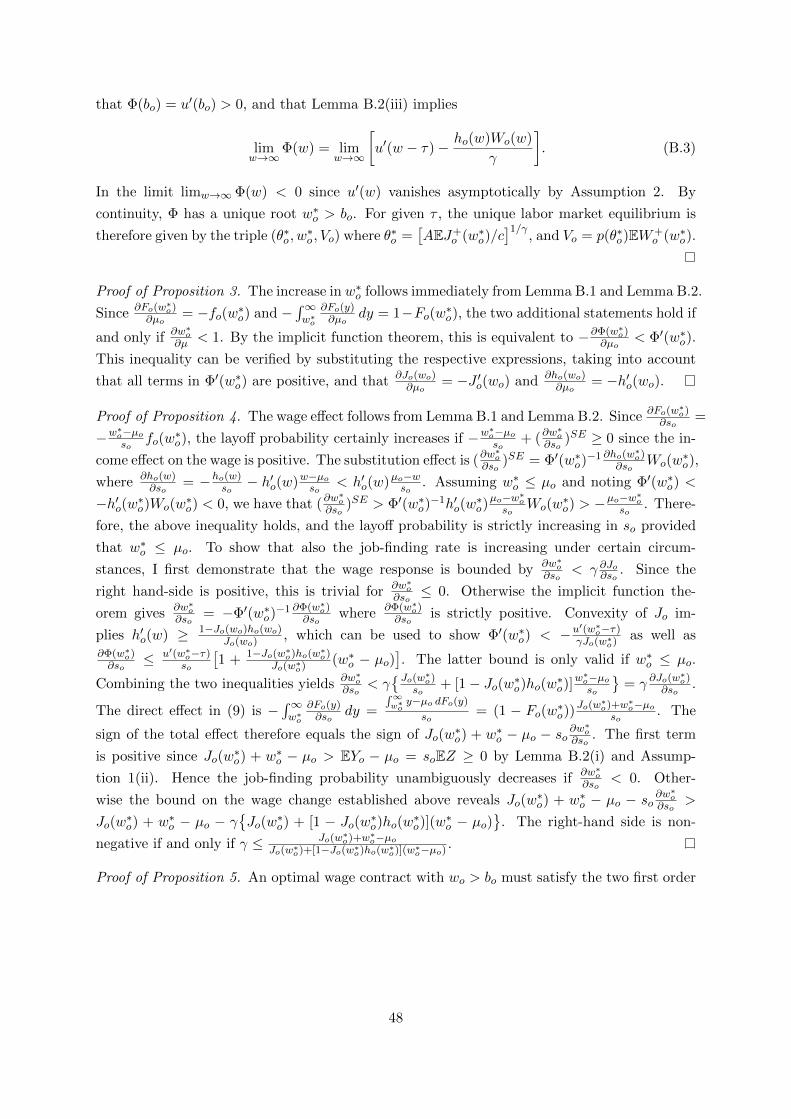
that Φ(bo) = u′(bo) > 0, and that Lemma B.2(iii) implies
limw→∞
Φ(w) = limw→∞
[u′(w − τ)− ho(w)Wo(w)
γ
]. (B.3)
In the limit limw→∞Φ(w) < 0 since u′(w) vanishes asymptotically by Assumption 2. By
continuity, Φ has a unique root w∗o > bo. For given τ , the unique labor market equilibrium is
therefore given by the triple (θ∗o , w∗o , Vo) where θ∗o =
[AEJ+
o (w∗o)/c]1/γ
, and Vo = p(θ∗o)EW+o (w∗o).
Proof of Proposition 3. The increase in w∗o follows immediately from Lemma B.1 and Lemma B.2.
Since ∂Fo(w∗o)∂µo
= −fo(w∗o) and −∫∞w∗o
∂Fo(y)∂µo
dy = 1−Fo(w∗o), the two additional statements hold if
and only if ∂w∗o∂µ < 1. By the implicit function theorem, this is equivalent to −∂Φ(w∗o)
∂µo< Φ′(w∗o).
This inequality can be verified by substituting the respective expressions, taking into account
that all terms in Φ′(w∗o) are positive, and that ∂Jo(wo)∂µo
= −J ′o(wo) and ∂ho(wo)∂µo
= −h′o(wo).
Proof of Proposition 4. The wage effect follows from Lemma B.1 and Lemma B.2. Since ∂Fo(w∗o)∂so
=
−w∗o−µoso
fo(w∗o), the layoff probability certainly increases if −w∗o−µo
so+ (∂w
∗o
∂so)SE ≥ 0 since the in-
come effect on the wage is positive. The substitution effect is (∂w∗o
∂so)SE = Φ′(w∗o)
−1 ∂ho(w∗o)
∂soWo(w
∗o),
where ∂ho(w)∂so
= −ho(w)so− h′o(w)w−µoso
< h′o(w)µo−wso. Assuming w∗o ≤ µo and noting Φ′(w∗o) <
−h′o(w∗o)Wo(w∗o) < 0, we have that (∂w
∗o
∂so)SE > Φ′(w∗o)
−1h′o(w∗o)µo−w∗oso
Wo(w∗o) > −
µo−w∗oso
. There-
fore, the above inequality holds, and the layoff probability is strictly increasing in so provided
that w∗o ≤ µo. To show that also the job-finding rate is increasing under certain circum-
stances, I first demonstrate that the wage response is bounded by ∂w∗o∂so
< γ ∂Jo∂so. Since the
right hand-side is positive, this is trivial for ∂w∗o∂so≤ 0. Otherwise the implicit function the-
orem gives ∂w∗o∂so
= −Φ′(w∗o)−1 ∂Φ(w∗o)
∂sowhere ∂Φ(w∗o)
∂sois strictly positive. Convexity of Jo im-
plies h′o(w) ≥ 1−Jo(wo)ho(wo)Jo(wo)
, which can be used to show Φ′(w∗o) < −u′(w∗o−τ)γJo(w∗o) as well as
∂Φ(w∗o)∂so
≤ u′(w∗o−τ)so
[1 + 1−Jo(w∗o)ho(w∗o)
Jo(w∗o) (w∗o − µo)]. The latter bound is only valid if w∗o ≤ µo.
Combining the two inequalities yields ∂w∗o∂so
< γ{Jo(w∗o)
so+ [1− Jo(w∗o)ho(w∗o)]
w∗o−µoso
}= γ ∂Jo(w
∗o)
∂so.
The direct effect in (9) is −∫∞w∗o
∂Fo(y)∂so
dy =
∫∞w∗o
y−µo dFo(y)
so= (1 − Fo(w∗o))
Jo(w∗o)+w∗o−µoso
. The
sign of the total effect therefore equals the sign of Jo(w∗o) + w∗o − µo − so
∂w∗o∂so
. The first term
is positive since Jo(w∗o) + w∗o − µo > EYo − µo = soEZ ≥ 0 by Lemma B.2(i) and Assump-
tion 1(ii). Hence the job-finding probability unambiguously decreases if ∂w∗o∂so
< 0. Other-
wise the bound on the wage change established above reveals Jo(w∗o) + w∗o − µo − so
∂w∗o∂so
>
Jo(w∗o) + w∗o − µo − γ
{Jo(w
∗o) + [1 − Jo(w
∗o)ho(w
∗o)](w
∗o − µo)
}. The right-hand side is non-
negative if and only if γ ≤ Jo(w∗o)+w∗o−µoJo(w∗o)+[1−Jo(w∗o)ho(w∗o)](w∗o−µo)
.
Proof of Proposition 5. An optimal wage contract with wo > bo must satisfy the two first order
48
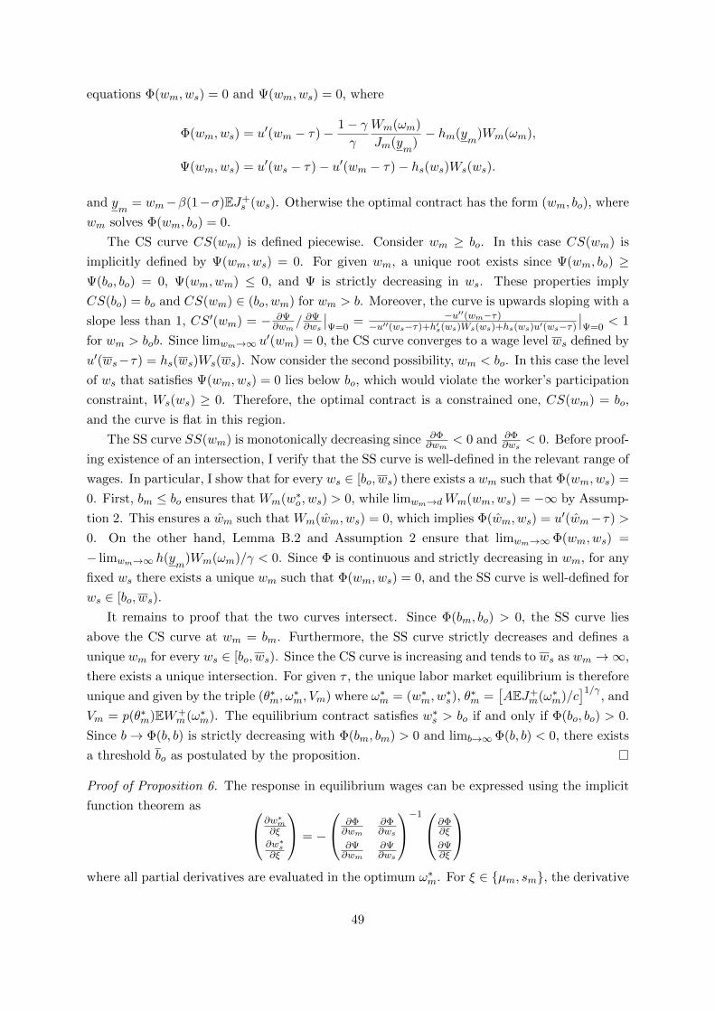
equations Φ(wm, ws) = 0 and Ψ(wm, ws) = 0, where
Φ(wm, ws) = u′(wm − τ)− 1− γγ
Wm(ωm)
Jm(ym
)− hm(y
m)Wm(ωm),
Ψ(wm, ws) = u′(ws − τ)− u′(wm − τ)− hs(ws)Ws(ws).
and ym
= wm−β(1−σ)EJ+s (ws). Otherwise the optimal contract has the form (wm, bo), where
wm solves Φ(wm, bo) = 0.
The CS curve CS(wm) is defined piecewise. Consider wm ≥ bo. In this case CS(wm) is
implicitly defined by Ψ(wm, ws) = 0. For given wm, a unique root exists since Ψ(wm, bo) ≥Ψ(bo, bo) = 0, Ψ(wm, wm) ≤ 0, and Ψ is strictly decreasing in ws. These properties imply
CS(bo) = bo and CS(wm) ∈ (bo, wm) for wm > b. Moreover, the curve is upwards sloping with a
slope less than 1, CS′(wm) = − ∂Ψ∂wm
/ ∂Ψ∂ws
∣∣Ψ=0
= −u′′(wm−τ)−u′′(ws−τ)+h′s(ws)Ws(ws)+hs(ws)u′(ws−τ)
∣∣Ψ=0
< 1
for wm > bob. Since limwm→∞ u′(wm) = 0, the CS curve converges to a wage level ws defined by
u′(ws−τ) = hs(ws)Ws(ws). Now consider the second possibility, wm < bo. In this case the level
of ws that satisfies Ψ(wm, ws) = 0 lies below bo, which would violate the worker’s participation
constraint, Ws(ws) ≥ 0. Therefore, the optimal contract is a constrained one, CS(wm) = bo,
and the curve is flat in this region.
The SS curve SS(wm) is monotonically decreasing since ∂Φ∂wm
< 0 and ∂Φ∂ws
< 0. Before proof-
ing existence of an intersection, I verify that the SS curve is well-defined in the relevant range of
wages. In particular, I show that for every ws ∈ [bo, ws) there exists a wm such that Φ(wm, ws) =
0. First, bm ≤ bo ensures that Wm(w∗o , ws) > 0, while limwm→dWm(wm, ws) = −∞ by Assump-
tion 2. This ensures a wm such that Wm(wm, ws) = 0, which implies Φ(wm, ws) = u′(wm− τ) >
0. On the other hand, Lemma B.2 and Assumption 2 ensure that limwm→∞Φ(wm, ws) =
− limwm→∞ h(ym
)Wm(ωm)/γ < 0. Since Φ is continuous and strictly decreasing in wm, for any
fixed ws there exists a unique wm such that Φ(wm, ws) = 0, and the SS curve is well-defined for
ws ∈ [bo, ws).
It remains to proof that the two curves intersect. Since Φ(bm, bo) > 0, the SS curve lies
above the CS curve at wm = bm. Furthermore, the SS curve strictly decreases and defines a
unique wm for every ws ∈ [bo, ws). Since the CS curve is increasing and tends to ws as wm →∞,
there exists a unique intersection. For given τ , the unique labor market equilibrium is therefore
unique and given by the triple (θ∗m, ω∗m, Vm) where ω∗m = (w∗m, w
∗s), θ
∗m =
[AEJ+
m(ω∗m)/c]1/γ
, and
Vm = p(θ∗m)EW+m(ω∗m). The equilibrium contract satisfies w∗s > bo if and only if Φ(bo, bo) > 0.
Since b→ Φ(b, b) is strictly decreasing with Φ(bm, bm) > 0 and limb→∞Φ(b, b) < 0, there exists
a threshold bo as postulated by the proposition.
Proof of Proposition 6. The response in equilibrium wages can be expressed using the implicit
function theorem as ∂w∗m∂ξ
∂w∗s∂ξ
= −
∂Φ∂wm
∂Φ∂ws
∂Ψ∂wm
∂Ψ∂ws
−1 ∂Φ∂ξ
∂Ψ∂ξ
where all partial derivatives are evaluated in the optimum ω∗m. For ξ ∈ {µm, sm}, the derivative
49

∂Ψ∂ξ is zero and we can rewrite
(∂w∗m∂ξ ,
∂w∗s∂ξ
)′=(− ∂Ψ
∂ws, ∂Ψ∂wm
)′ ∂Φ∂ξD
−1 where D = ∂Φ∂wm
∂Ψ∂ws−
∂Φ∂ws
∂Ψ∂wm
> 0 is the determinant of the Jacobian. Since the entries of the vector on the right-
hand side are all positive, the two wage levels move in the same direction, and the sign of∂w∗i∂ξ equals the sign of ∂Φ
∂ξ . Lemma B.1 and Lemma B.2 imply that ∂Φ∂µm
> 0 such that the
equilibrium wages increase in µm, while the wage effect of sm is ambiguous.
The effects of an arbitrary parameter ξ on layoffs and hiring are similar to (8)–(9)
dFm(y∗m
)
dξ=∂Fm(y∗
m)
∂ξ+ fm(y∗
m)∂y∗
m
∂ξ,
dFs(w∗s)
dξ=∂Fs(w
∗s)
∂ξ+ fs(w
∗s)∂w∗s∂ξ
,
dEJ+m(ω∗m)
dξ= −
∫ ∞y∗m
∂Fm(y)
∂ξdy − (1− Fm(y∗
m))∂y∗
m
∂ξ.
For ξ ∈ {µm, sm}, the change in the layoff probability of senior workers is proportional to their
wage response, dFs(w∗s )dξ = fs(w
∗s)∂w∗s∂ξ , whereby dFs(w∗s )
dµm> 0. By the definition of y∗
m, observe
∂y∗m
∂ξ=∂w∗m∂ξ
+ β(1− Fs(w∗s))∂w∗s∂ξ
=− ∂Ψ∂ws
+ β(1− σ)(1− Fs(w∗s)) ∂Ψ∂wm
D
∂Φ
∂ξ. (B.4)
Straightforward differentiation reveals that in optimum ∂Φ∂ws
= β(1 − σ)(1 − Fs(w∗s))[∂Φ∂wm
−u′′(w∗m − τ)
]. The determinant can therefore be rewritten D = − ∂Φ
∂wm[− ∂Ψ
∂ws+ β(1 − σ)(1 −
Fs(w∗s))
∂Ψ∂wm
] + β(1 − σ)(1 − Fs(w∗s))u
′′(w∗m − τ) ∂Ψ∂wm
. Substituting this into (B.4) and not-
ing u′′ < 0 reveals that∂y∗m
∂ξ = λ(−∂Φ∂ξ )/ ∂Φ
∂wm= λ∂w
∗m
∂ξ
∣∣ws=w∗s
for a λ ∈ (0, 1). The proofs
of Proposition 3 and Proposition 4 can be replicated to show that ∂w∗m∂µm
∣∣ws=w∗s
∈ (0, 1) and
∂w∗m∂sm
∣∣ws=w∗s
≤ γ ∂Jm(y∗m
)
∂sm. Since λ ∈ (0, 1), the same bounds hold for
∂y∗m
∂µmand
∂y∗m
∂sm. The remain-
der of the proof is then analogous to that of Proposition 3 and Proposition 4.
Proof of Proposition 7. I demonstrate that the assumption on γ is sufficient for the SS curve to
shift upwards if µs increases. The SS curve shifts upwards at the optimum if and only if ∂Φ(ω∗m)∂µs
=
∂Φ(ω∗m)∂Wm
∂Wm(ω∗m)∂µs
+ ∂Φ(ω∗m)∂ym
∂y∗m
∂µs> 0. It is easy to verify that ∂Φ(ω∗m)
∂Wm= −u′(w∗m−τ)
Wm(ω∗m) , and that the
convexity of the conditional expectation Jm implies ∂Φ(ω∗m)∂ym
<J ′m(y∗
m)
Jm(y∗m
)u′(w∗m − τ). Furthermore,
∂Wm(ω∗m)∂µs
= β(1−σ)fs(w∗s)Ws(w
∗s) and
∂y∗m
∂µs= −β(1−σ)(1−Fs(w∗s)). Combining all of the above
yields ∂Φ(ω∗m)∂µs
> −β(1− σ)(1− Fs(w∗s))u′(w∗m − τ)[hs(w∗s )Ws(w∗s )Wm(ω∗m) +
J ′m(y∗m
)
Jm(y∗m
)
]. The term in square
brackets has the same sign as J ′m(y∗m
)Wm(ω∗m)Jm(y∗
m) + hs(w
∗s)Ws(w
∗s) = hm(y∗
m)Wm(ω∗m)− Wm(ω∗m)
Jm(y∗m
) +
hs(w∗s)Ws(w
∗s) = u′(w∗s − τ) − 1
γWm(ω∗m)Jm(y∗
m) , where the last identity exploits the two optimality
conditions. The assumption on γ postulated by Proposition 7 therefore ensures ∂Φ(ω∗m)∂µs
> 0.
Proof of Proposition 9. Since Jo(w•o(y); y) > 0 only for y > y•
o, expected firm surplus can be
rewritten as EJ+o (w•o) =
∫∞yroJo(w
•o ; y) dFo(y) =
E[Yo−y•o|Yo≥y•o]
1−βo(1−φ) . Since w•o(yro) = yro +βφEJ+
o (w•o),
equation (5) reveals yo(w•o(yr)) = yro. Monotonicity then implies y∗
o= y
o(w∗o) > yro. By the free
entry conditions (6) and (19), the job-finding probability is only a function of expected firm
50

surplus EJ+o . Define I(a) =
∫∞a 1−Fo(y) dy
1−βo(1−φ) , which is strictly decreasing in a. Under the friction,
EJ+o (w∗o) = I(y
o(w∗o)), while without the friction, EJ+
o (w•o) = I(yo(w•o)). Since y
ois strictly
increasing and w∗o < w•o by assumption, we have EJ+o (w∗o) > EJ+
o (w•o).
C Equilibrium with labor market policies
C.1 Surplus functions and optimality conditions
To study different labor market policies in Section 6.4, the model of Section 4 is extended by
the following elements,
• a training program that changes the productivity distribution Fi and costs the public Ci
per participant,
• a firm that employs a type i worker receives a wage cost subsidy Si,
• a firm that (endogenously) lays off a type i worker pays a layoff tax Ti to the government,
and severance pay Pi to the displaced worker.
I only discuss the changes regarding old workers at this place. The same modifications apply
to prime-age and senior workers. Due to the wage subsidy, an old worker earns wo but costs
the firm only wo − So. This changes firm surplus at the production stage to
Jo(wo; y) =y − (wo − So) + βoφEJ+
o (wo)
1− βo(1− φ).
Due to the layoff tax and the severance pay, the worker is laid off whenever Jo(wo; y)+To+Po < 0
which changes the layoff threshold to yo(wo) = wo−So−βoφEJ+
o (wo)−(1−βo(1−φ))(To+Po).
This allows to express firm surplus as Jo(wo; y) =y−y
o(wo)
1−βo(1−φ) − (To +Po). Expected firm surplus
has to take into account that for y < yo(wo) the firm incurs layoff costs,
EJ+o (wo) =
∫∞yo
y − yodFo(y)
1− βo(1− φ)− (To + Po).
This yields the implicit equation for the layoff threshold
yo− (wo − So) +
βoφ
1− βo(1− φ)
∫ ∞yo
y − yodFo(y) + (1− βo)(To + Po) = 0.
Worker surplus at the production stage is Wo(wo) = u(wo−τ)−u(bo−τ)+βo(EW+o (wo)−Vo)
1−βo(1−φ) , while
expected surplus is EW+o (wo) = (1 − Fo(yo))Wo(wo) + Fo(yo)(u(bo + Po − τ) − u(bo − τ)).
51

Substituting Wo(wo) yields
EW+o (wo) = (1− Fo(yo)
u(wo − τ)− u(bo − τ)− βoVo1− βo(1− φFo(yo))
+ Fo(yo)(1− βo(1− φ))u(bo + Po − τ)− u(bo − τ)
1− βo(1− φFo(yo)).
The first order condition (5) becomes
u′(w∗o − τ) =1− γγ
EW+o (w∗o)
EJ+o (w∗o)
+ (1− βo(1− φ))ho(y∗o)∂y∗
o
∂wo[Wo(w
∗o) + u(bo − τ)− u(bo + Po − τ)]
wherey∗o
∂wo= 1−βo(1−φ)
1−βo(1−φFo(y∗o)) . Similar changes apply to the surplus functions of prime-age and
senior workers and the first order conditions for ωm. In the aggregate, wage subsidies, training,
and layoff taxes change the composition of government expenditures,
G1 = (N1 − Em)gm + EmSm − LmTm − Cmp(θ∗m)Qm,
G2 = (N2 − Es − Eo)go + EsSs + EoSo − LsTs − LoTo − Csπm(1− σ)Em − p(θ∗o)Qo,
where Li amounts to the mass of layoff events involving type i workers,
Lm = [JSmp(θ∗m) + (1− πm)(1− σ)φEm]Fm(y∗
m),
Ls = [πm(1− σ)Em + (1− πo)(1− σ)(1− δ)φEs]Fs(y∗s),
Lo = [JSop(θ∗o) + (1− πo)(1− σ)(1− δ)φEo]Fo(y∗o),
and Qi denotes the mass of type i individuals who have not been employed in their age class
before, which satisfy
Qm = πmN1 + (1− πm)(1− p(θ∗m))Qm,
Qo = πm(1− p(θ∗o))[N1 − (1− σ)Em] + (1− πo)(1− δ)(1− p(θ∗o))Qo.
Severance pay directly affects welfare, which is updated to
W1 = Emu(w∗m − τ) + (N1 − Em − Lm)u(bm − τ) + Lmu(bm + Pm − τ),
W2 = Esu(w∗s − τ) + Eou(w∗o − τ) + (N2 − Eo − Es − Lo − Ls)u(bo − τ)
+ Lsu(bp + Ps − τ) + Lou(bo + Po − τ).
52

C.2 Quantitative effects
Figure C.1: effect of severance pay on employment, output and welfare, relative to Table 4(a); only onevariable is altered at a time; solid line: Pm, dashed line: Ps, dash-dotted line: Po
Figure C.2: effect of severance pay with a probation period on employment, output and welfare, relativeto Table 4(a); only one variable is altered at a time; solid line: Pm, dashed line: Ps, dash-dotted line: Po
53
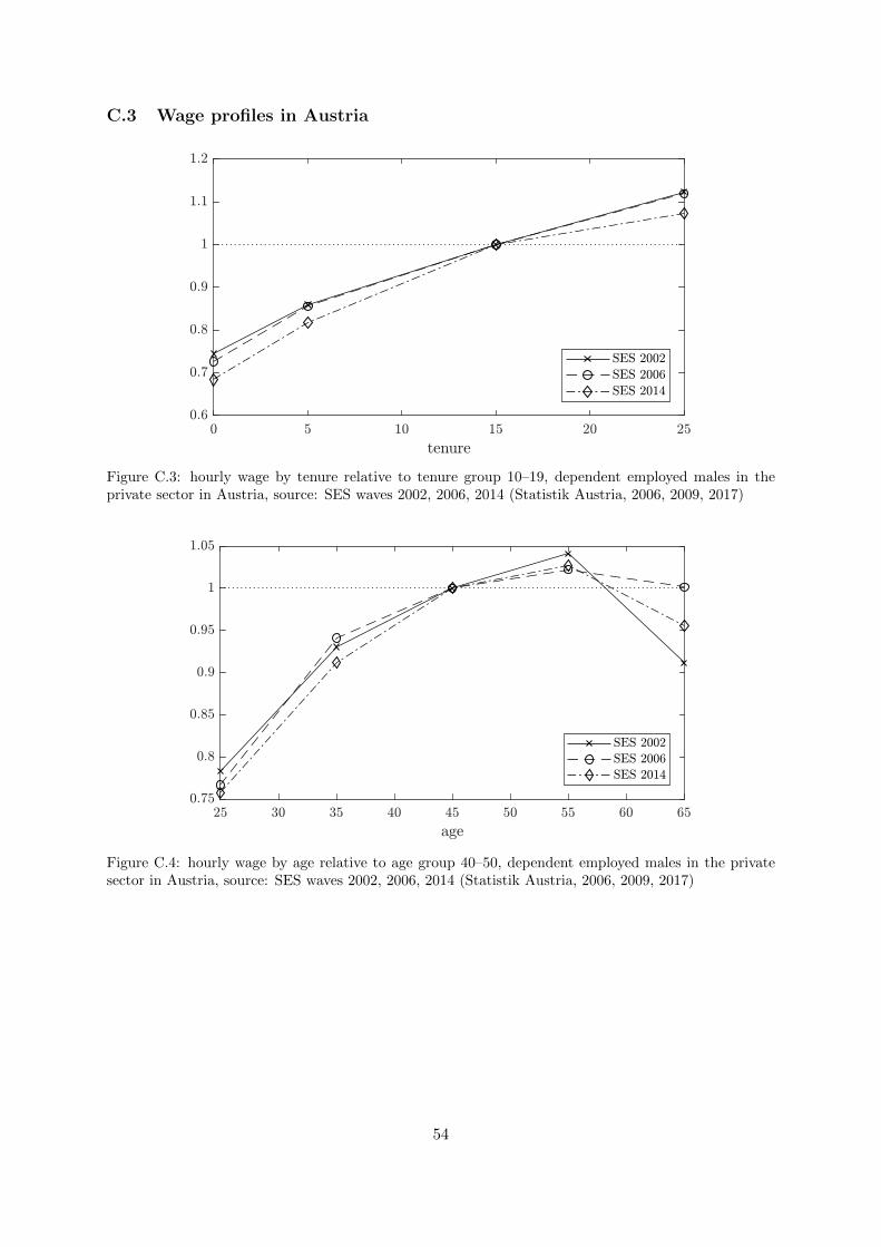
C.3 Wage profiles in Austria
Figure C.3: hourly wage by tenure relative to tenure group 10–19, dependent employed males in theprivate sector in Austria, source: SES waves 2002, 2006, 2014 (Statistik Austria, 2006, 2009, 2017)
Figure C.4: hourly wage by age relative to age group 40–50, dependent employed males in the privatesector in Austria, source: SES waves 2002, 2006, 2014 (Statistik Austria, 2006, 2009, 2017)
54