ABSTRACT

Title of dissertation: INFORMATIONAL FRICTIONS AND LEARNINGIN EMERGING MARKETS

Emine Boz, Doctor of Philosophy, 2006

Dissertation directed by: Professor Enrique G. Mendoza

Department of Economics

Emerging market financial crises are abrupt and dramatic, usually occurring

after a period of high output growth, massive capital flows, and a boom in asset

markets. This thesis develops an equilibrium asset pricing model with informational

frictions in which vulnerability and the crisis itself are consequences of the investor

optimism in the period preceding the crisis. The model features two sets of investors,

domestic and foreign. Both sets of investors are imperfectly informed about the true

state of the emerging economy. Investors learn from noisy signals which contain

information relevant for asset returns and formulate expectations, or “beliefs”, about

the state of productivity.

Numerical analysis shows that, if preceded by a sequence of positive signals, a

small, negative noise shock can trigger a sharp downward adjustment in investors’

beliefs, asset prices, and consumption. The magnitude of this downward adjust-

ment and sensitivity to negative signals increase with the level of optimism attained

prior to the negative signal. The model calibrated to a typical emerging market

economy, Turkey, reveals that with the introduction of incomplete information asset

prices display persistent effects in response to transitory shocks, and the volatility

of consumption increases by 2.1 percentage points.

The maximum likelihood estimation of the model’s parameters using U.S. data

documents that the estimated signal-to-noise ratio for the U.S. is higher since, unlike

Turkey, a significantly higher portion of fluctuations can be accounted for by changes

in the persistent component rather than the noise. Feeding these two different

signal-to-noise ratios to the model, we find that the booms and busts driven by

misperceptions of the investors have significantly lower frequency, magnitude, and

duration in the case of U.S. compared to Turkey.

INFORMATIONAL FRICTIONS AND LEARNING INEMERGING MARKETS

by

EMINE BOZ

Dissertation submitted to the Faculty of the Graduate School of theUniversity of Maryland, College Park in partial fulfillment

of the requirements for the degree ofDoctor of Philosophy

2006

Advisory Commmittee:

Professor Enrique G. Mendoza, ChairProfessor John RustProfessor Guillermo A. CalvoProfessor Carlos VeghProfessor Haluk Unal

c© Copyright by

Emine Boz

2006

DEDICATION

To my father and my husband.

ii

ACKNOWLEDGMENTS

Many thanks to Enrique Mendoza, John Rust, Guillermo Calvo, Carlos Vegh,

and Haluk Unal for kindly accepting to serve on my committee.

My special thanks go to my mentor Enrique Mendoza, who helped me discover

who I am, and who I want to be while I took my first steps in the journey of economic

research. He never lost confidence in me even when my self-confidence was shaken.

I am grateful for his continuous support not only on my research but also on many

other aspects of life.

My thanks also go to my mentor John Rust for his always encouraging and

supportive advise and his positive attitude. It has been a great experience to learn

from him and to work with him. In addition, thanks are due to Guillermo Calvo

for letting me benefit from his vast knowledge and experience in economics. Also,

to the rest of the international finance team particulary to Carlos Vegh for his very

useful comments, Christian Daude, Irani Arraiz, and Ran Bi for their suggestions

and support along the way.

I owe my deepest thanks to my husband, Bora, for always holding my hand

as we travelled this journey together. In this difficult process, I realized how lucky I

was to have his companionship both in the journey of research and of life especially

when these two became inseparable. Every time I got stuck thinking about the

empty half of the glass, he was there to remind me that the other half was full.

iii

My gratitude also go to all friends and relatives whose birthdays, weddings,

and many other important events I missed. Also, to my mother for understanding

and respecting my priorities even if this meant that her only daughter would become

mainly a voice on the phone. And finally, thanks to my father who was the first

person to realize that I actually “enjoyed” studying and who would be so proud if

he had lived to see this day.

iv

TABLE OF CONTENTS

List of Tables vi

List of Figures vii

1 Introduction 1

2 Model 102.1 Domestic Households’ Problem . . . . . . . . . . . . . . . . . . . . . 102.2 Foreign Investors’ Problem . . . . . . . . . . . . . . . . . . . . . . . . 122.3 Information Structure . . . . . . . . . . . . . . . . . . . . . . . . . . 13

3 Quantitative Analysis 223.1 Computation . . . . . . . . . . . . . . . . . . . . . . . . . . . . . . . 223.2 Calibration . . . . . . . . . . . . . . . . . . . . . . . . . . . . . . . . 243.3 Quantitative Findings . . . . . . . . . . . . . . . . . . . . . . . . . . 273.4 From Miracles to Crises . . . . . . . . . . . . . . . . . . . . . . . . . 383.5 Turkey vs. U.S. . . . . . . . . . . . . . . . . . . . . . . . . . . . . . . 403.6 Sensitivity Analysis . . . . . . . . . . . . . . . . . . . . . . . . . . . . 44

4 Asymmetric Information 474.1 Quantitative Analysis . . . . . . . . . . . . . . . . . . . . . . . . . . . 49

5 Conclusion 53

A Proofs 56

Bibliography 61

v

LIST OF TABLES

1.1 Magnitudes of pre-crisis booms. . . . . . . . . . . . . . . . . . . . . . 3

3.1 Model parameters . . . . . . . . . . . . . . . . . . . . . . . . . . . . . 25

3.2 Long-run business cycle moments, simulated data is logged and HPfiltered. . . . . . . . . . . . . . . . . . . . . . . . . . . . . . . . . . . 29

3.3 Analysis of optimism (pessimism) driven booms (busts). . . . . . . . 36

3.4 U.S. vs Turkey, parameters . . . . . . . . . . . . . . . . . . . . . . . . 42

3.5 U.S. vs Turkey, booms and busts . . . . . . . . . . . . . . . . . . . . 43

3.6 Sensitivity analysis, simulated data is logged and linearly detrended. . 45

4.1 Simulations for the asymmetric information setup; simulated data arelogged and linearly detrended. . . . . . . . . . . . . . . . . . . . . . . 51

vi

LIST OF FIGURES

2.1 Density of dt conditional on zt. . . . . . . . . . . . . . . . . . . . . . 17

2.2 Next period’s beliefs zt+1 = φ(zt, dt+1) for three different values ofcurrent beliefs zt. . . . . . . . . . . . . . . . . . . . . . . . . . . . . . 18

2.3 The derivative of φ(zt, dt+1) with respect to dt+1 as a function of zt. . 21

3.1 Ergodic distribution of domestic investors’ asset holdings, α, in thecase of (a) full information, and (b) incomplete information. . . . . . 28

3.2 Ergodic distribution of beliefs, z. . . . . . . . . . . . . . . . . . . . . 28

3.3 Time series simulation for the case of full information. . . . . . . . . . 31

3.4 Time series simulation for the case of incomplete information. . . . . 32

3.5 Forecasting functions conditional on α = 0.840, d = zL, z = zH (firstcolumn), and z = zL (second column). . . . . . . . . . . . . . . . . . 34

3.6 Sequences of positive signals . . . . . . . . . . . . . . . . . . . . . . . 39

3.7 Time series simulations for U.S. and Turkey. . . . . . . . . . . . . . . 41

vii

Chapter 1

Introduction

...That this region [East Asia] might become embroiled in one of the worst

financial crises in the postwar period was hardly ever considered-within

or outside the region-a realistic possibility. What went wrong? Part of

the answer seems to be that these countries became victims of their own

success. This success had led domestic and foreign investors to underes-

timate the countries economic weaknesses. It had also, partly because of

the large scale financial inflows that it encouraged, increased the demands

on policies and institutions, especially but not only in the financial sec-

tor; and policies and institutions had not kept pace. The fundamental

policy shortcomings and their ramifications were fully revealed only as

the crisis deepened... IMF (1998)

The experience of the last decade suggests that emerging capital markets are

vulnerable to significant shifts in investors’ confidence in both upward and downward

directions. Downward shifts in confidence and financial market collapses are abrupt

and often take place unexpectedly after a large boom. Table 1.1 documents the

magnitude of these booms for several pre-crisis episodes: Argentina and Mexico in

1994, Korea in 1997, and Turkey in 2000. Taking Turkey as an example, the year

before its financial crisis in 2001, the country boasted an average quarterly current

1

account-to-GDP ratio of -5.1%, private consumption growth of 4.5%, an increase in

equity prices of 57% and GDP growth of 3%.1

It is widely agreed that overconfidence and informational problems are at

least partially responsible for recent crisis episodes, as the above opening quote by

International Monetary Fund on the Asian crisis suggests. Whether these frictions

in international capital markets can be large enough to explain pre-crisis periods of

bonanza and the depth of the crises remains an open question.

In this thesis, we aim to answer this question by studying the quantitative

predictions of a model in which optimism, due to investors’ underestimation of

the weaknesses of emerging economies, acts as the driving force behind both the

pre-crisis booms and the vulnerability that paves the way to financial turmoil and

deep recessions. In the model, the pre-crisis bonanza is driven by a sequence of

positive signals that investors interpret as an improvement in the true fundamentals

of the economy. The crisis occurs as a sudden downward adjustment in investors’

expectations of the true fundamentals is triggered and their optimism suddenly

fades. Furthermore, the magnitude of the adjustment increases with the level of

optimism attained prior to the crisis.

The informational frictions that are the key ingredient of the model, are likely

to be prevalent in emerging markets for several reasons. One is the lack of trans-

parency in policy-making, and data reporting which manifests itself in the form of

inaccurate or misleading data. In a report, the International Monetary Fund argued

1Calvo and Reinhart (2000) conclude that “Sudden Stops,” sharp negative reversals of capitalflows, are usually preceded by a surge in capital inflows.

2

Table 1.1: Magnitudes of pre-crisis booms.

Episode GDP (%) Consumption (%) Equity Price (%) CA/GDP (%)

Argentina, 1994Q1-Q4 1.72 2.67 12.97 -1.08

Mexico, 1994Q1-Q4 3.43 6.69 18.53 -2.00

Korea, 1996Q4-1997Q3 3.67 5.14 1.04 -3.69

Turkey, 2000Q1-Q4 3.08 4.51 57.30 -5.12

Average quarterly changes in GDP, private consumption, equity prices and average quarterlycurrent account-to-GDP ratios. GDP, and consumption are in constant prices, equity prices arein local currencies and are deflated using the CPI. Source: International Financial Statistics andcorresponding countries’ central banks.

that this was a common thread running through several recent crisis episodes:

... A lack of transparency was a feature of the build-up to the Mexican

crisis of 1994-95 and of the emerging market crises of 1997-98. In these

crises, markets were kept in the dark about important developments

and became first uncertain and then unnerved as a host of interrelated

problems came to light. Inadequate economic data, hidden weaknesses

in financial systems, and a lack of clarity about government policies and

policy formulation contributed to a loss of confidence that ultimately

threatened to undermine global stability ...(2001)

A second reason informational frictions pose particular challenges for emerging

economies is the existence of high fixed costs associated with obtaining country-

specific information and keeping up with the developments in emerging economies,

as suggested by Calvo (1999). Such costs could arise due to idiosyncrasies affecting

financial markets in these countries, including for example, each country’s unique

3

institutions, policies, political environment, legal structure, etc. In addition, it might

be optimal for international investors not to “buy” this information. Calvo and

Mendoza (2000) provide two arguments for why this can be the case. First, if short

selling positions are limited, the benefit of paying for costly information declines

as the number of emerging economies in which to invest becomes sufficiently large.

Second, if punishment for poor performance is high, managers of investment funds

may choose to mimic each other’s behavior instead of paying for costly information.

The model in this thesis features two types of investors, domestic and for-

eign, both of whom trade a single emerging market asset. Domestic investors are

consumer-investors who maximize the expected present discounted value of their

lifetime utility. Foreign investors specialize in trading the emerging market asset,

face trading costs, and maximize the expected present discounted value of profits

from investing. We model the informational frictions as follows. Both sets of in-

vestors are imperfectly informed about the true state of current productivity, which

contains information relevant for predicting future returns on the emerging market

asset. They can only partially infer the true state of productivity by “learning” from

publicly observed dividends (or signals) and, they share the same information set.

The dividends consist of two parts: a persistent component, which we interpret as

“true productivity”, and a transitory component, which is a noise term that controls

the accuracy of the signals. Modeled in this way, dividends serve an informational

role since a dividend payment is a noisy signal that contains information about

current and future realizations of productivity. Every period, foreign and domestic

investors observe dividends, solve a signal extraction problem, and “learn” about

4

productivity by updating their expectations or “beliefs” regarding true productivity.

When investors turn pessimistic (optimistic), asset prices are driven below

(above) the “fundamentals price,” which is defined as the expected present dis-

counted value of dividends conditional on full information. In these periods, asset

prices and domestic investors’ consumption display swings that are not associated

with changes in true productivity. We find that a sequence of positive signals can

cause a boom in both the asset market and in consumption, and can be a source

of economic vulnerability if true productivity is in fact low. If a negative signal is

realized at the peak of a boom of this nature and, as a result, “challenges” current

prevailing beliefs, an abrupt and large downward adjustment in asset prices and

consumption takes place. If, however, the same signal “confirms” prevailing beliefs,

its impact is smaller.2

Foreign and domestic investors trade due to differences in their objective func-

tions particularly their risk aversions, but not for speculation (given that they have

the same beliefs). From the domestic investors’ perspective, dividend shocks are

important for two reasons. First, in order to intertemporally smooth consumption

domestic investors would like to increase (decrease) their asset position in response

to positive (negative) dividend shocks. Second, they play a critical informational

role. In response to a negative dividend shock, changes in expectations due to the

new information compounds the first effect, and as result, domestic investors reduce

their demand for the emerging market asset. Foreign investors also reduce their

2Moore and Schaller (2002) establish the state dependence of responses to noisy signals. Weborrow our terminology from them.

5

demand for the asset in response to this shock, since they receive a negative signal

regarding future productivity. In equilibrium, we find that domestic investors’ de-

mand decreases by more than that of their foreign counterparts, therefore, domestic

investors become net sellers in response to a negative dividend shock. This result

leads to a procyclical current account on average. However, we also find that for

a given dividend shock, the higher the expectations about future productivity, the

lower are the domestic investors’ asset holdings since higher expectations induce

foreign investors to bid more aggressively, compared to their risk-averse domestic

counterparts, for the same asset. Hence, the higher the investment optimism, the

more the emerging economy can attract foreign investment, and therefore the more

likely the country is to develop a potentially sizable current account deficit. For

a given dividend shock, the model can thus produce a current account deficit and

booms in consumption and asset prices if investors are “sufficiently optimistic”.

The numerical analysis shows that with the introduction of informational fric-

tions, the volatility of the emerging economy’s consumption increases by 2 percent-

age points compared to the “full information” setup. Uncertainty about true cur-

rent productivity leads to increased uncertainty regarding future asset returns and a

more volatile consumption profile for the risk averse domestic investors. Moreover,

informational frictions produce persistence in response to transitory noise shocks.

If investors turn pessimistic (optimistic) in response to a misleading signal, it takes

several periods for them to correct their beliefs. The mechanism behind this re-

sult is the Bayesian learning process: the posteriors of one period are used in the

calculation of the following period’s priors.

6

We calibrate the benchmark incomplete information model and pin down the

signal-to-noise ratio using Turkish GDP data. Conducting the same calibration ex-

ercise with U.S. data reveals that the signal-to-noise ratio for this country is signifi-

cantly higher, confirming that informational frictions are more prevalent in emerging

market economies rather than the developed. The calibration exercise conducting

using a maximum likelihood estimation procedure similar to Hamilton (1989) al-

lows us to quantify this difference. The model calibrated for Turkey generates more

frequent, larger and longer booms and busts driven by investors’ misperceptions

compared to U.S.

This thesis is at the crossroads of two main strands of literature. The first

is the literature on Sudden Stops and financial crises in open economies, and the

second is that on informational frictions in finance. Most existing models of financial

crises and Sudden Stops, focus on crash episodes, but not on the booms preceding

the crashes that might indeed contain the seeds of the financial crises. In contrast,

the model proposed in this thesis accounts for the boom-bust cycles observed in

emerging markets. Studies explaining Sudden Stops focus on financial frictions and

often utilize collateral constraints, (see, for example, Caballero and Krishnamurthy

(2001), Paasche (2001), or Mendoza and Smith (2004)). Credit constraints are

successful for producing amplification in the response of the economy to typical

negative shocks. In this thesis, however, business cycles can also be driven by

changes in investor sentiment and amplification is at work in expansions as well as

in recessions.

In the international finance literature, shifts in investor sentiment have usually

7

been analyzed within the context of currency crises, often using sunspot models

that produce multiple equilibria. In this thesis, we take a different approach by

considering a model with a unique equilibrium that can endogenously produce shifts

in investors’ confidence and switches between good states and bad ones which allows

us to predict when these shifts occur and how long it takes for the market to recover

after a bust.

This thesis is also related to the literature on learning in macro and finance.

Particularly, Wang (1994), models dividends as noisy signals to analyze trading vol-

ume in stock markets, Albuquerque, Bauer and Schneider (2004) use noisy dividend

signals to investigate the effects of investor sophistication on international equity

flows, and Nieuwerburgh and Veldkamp (2004) use them to explain U.S. business

cycle asymmetries in an RBC framework with asymmetric learning.

In order to analyze whether the homogeneity of information plays a critical role

in the model, we also present a scenario in which investors are differentially informed.

This exercise is motivated by the findings of Calvo and Mendoza (2000). In this

“asymmetric information” setup, we assume that foreign investors are less informed

than domestic investors.3 Unlike their foreign counterparts, domestic investors are

assumed to know the true state of productivity: in other words, domestic investors

are perfectly informed. We conclude that it is sufficient to assume that one set of

3Empirical evidence about informational asymmetries between domestic and foreign investorsis mixed. Using data from Korea, Germany, Indonesia and China, Choe et al. (2000), Hau (2001),Dvorak (2001), Chan et al. (2003), and Chakravarty et al. (1998) find that domestic investors havemore valuable information than their foreign counterparts. On the other hand, Seasholes (2000),Grinblatt and Kelahaiju (2000), Wang and Stulz (1997) and Chui and Kwok (1998) use data forTaiwan, Finland, Japan and China and find that foreigners have more valuable information sincethey have the expertise that the domestic investors lack.

8

investors is imperfectly informed for the model to produce “misperception driven

cycles,” although the magnitude of these booms and busts would depend on the

proportion of imperfectly informed investors. (See Section 4 for details of this setup.)

The rest of the thesis proceeds as follows. We describe the model in Chapter

2, and in Chapter 3 we discuss the model’s solution procedure, calibration, and

numerical results. Chapter 4 goes on to investigate the implications of introducing

asymmetric information into the model. Finally, Chapter 5 concludes.

9

Chapter 2

Model

The economy has two classes of agents, foreign investors and domestic household-

investors, who are identical within each class. The domestic households maximize

expected lifetime utility by making consumption and asset holding decisions condi-

tional on their information set, that includes the noisy signals about the true state

of productivity. Foreign investors choose their asset positions in order to maximize

the expected present discounted value of profits based on their beliefs about the

state of productivity. Foreign investors also face trading costs associated with op-

erating in the asset market. Neither domestic nor foreign investors observe the true

realization of the stochastic productivity shock, which contains information relevant

for forecasting the returns from the asset. They only observe dividends, which are

noisy signals about the true value of productivity. Foreign and domestic investors

form their beliefs by solving a signal extraction problem.

2.1 Domestic Households’ Problem

Domestic households choose stochastic intertemporal plans for consumption,

ct, and asset holdings, αt+1, in order to maximize expected life-time utility condi-

10

tional on the information available to them:

U = E0

[ ∞∑t=0

βt c1−σt

1− σ|IU

0

](2.1)

subject to

ct + αt+1qt = αt(qt + dt) (2.2)

taking asset prices, qt, and the evolution of beliefs and their information set IU as

given.1 dt denotes dividend payments of the emerging market asset, the parameter σ

is the coefficient of relative risk aversion of domestic investors and β is the standard

subjective discount factor.

At the beginning of each period, productivity shocks are realized and dividends

are determined. Domestic investors make their decisions after observing dividends.

The optimality conditions characterizing their decisions are:

βtu′(ct)− λt = 0 (2.3)

−λtqt + Et[λt+1(dt+1 + qt+1)|IUt ] = 0 (2.4)

where λt denotes the Lagrange multiplier associated with the budget constraint.

Combining these two first order conditions gives the Euler equation:

qtu′(ct) = βEt

[(qt+1 + dt+1)u

′(ct+1)|IUt

]. (2.5)

1We discuss the role of the expectation operator and the information structure in Section 2.3.

11

This equation is familiar except that the expectations are taken conditional on the

information set IUt .

2.2 Foreign Investors’ Problem

As in Mendoza and Smith (2004), foreign investors choose {α∗t+1}∞0 in order

to maximize the expected present discounted value of their profits conditional on

their information sets:

E0

∞∑t=0

R−t(α∗t (dt + qt)− α∗t+1qt − qt

a

2(α∗t+1 − α∗t + θ)2|IU

0

)(2.6)

where R is the gross world interest rate, 1/a is the price elasticity of foreign investors’

demand, qta2(α∗t+1 − α∗t + θ)2 is the total trading cost associated with buying and

selling equities in the emerging economies, θ is the recurrent cost. As in Aiyagari and

Gertler (1999) and Mendoza and Smith (2004), we model the trading cost associated

with buying and selling the asset as quadratic in the size of the asset trade.2 The

first order condition of the foreign investors’ problem is:

qt

(1 + a(α∗t+1 − α∗t + θ)

)= R−1E

[dt+1 + qt+1(1 + a(α∗t+2 − α∗t+1 + θ))|IU

t

]. (2.7)

2This specification does not rule out buy & hold type of trading strategies. The foreign investorsare allowed to buy and “watch” the market and sell when they find it profitable to so. Theassumption that θ 6= 0 implies that “watching” the market also comes at a cost although it is lesscostly compared to trading. It is intuitive to assume that “watching” the market is costly as theinvestors still need to follow the developments in the emerging economy so as to determine theright time to sell. In Section 3.4, we do analyze the robustness of out results to this assumptionby solving the case in which θ = 0.

12

We can solve the above first order condition forward to obtain:

α∗t+1 − α∗t =1

a

(qbt

qt

− 1

)− θ. (2.8)

qbt , called the belief price, is defined as the expected present discounted value of

future dividends conditional on the current belief about productivity:

qbt ≡ E[R−1dt+1 + R−2dt+2 + R−3dt+3 + . . . |IU

t ]. (2.9)

Intuitively, foreign investors adjust their asset holdings “partially” depending on the

gap between the market price qt and their belief price qbt . How much of this gap is

reflected in the asset demand is determined by 1/a.

2.3 Information Structure

Dividends are determined exogenously as follows:

dt = ezt+ηt . (2.10)

There are two types of uncertainty associated with dividends: persistent aggregate

productivity shocks, z, and noise, in the form of transitory, additive, Normal i.i.d.

shocks, η, with E[η] = −σ2η/2 and E[η2] = σ2

η: η ∼ N(−σ2η/2, σ

2η).

3 Aggregate pro-

ductivity shocks follow a Markov process with two states and transition probability

matrix P . We denote the values z can take as z ∈ {zL, zH} and assume zL < zH

3This specification for E[η] guarantees that changes in ση produce mean preserving spreads.

13

without loss of generality.

Assumption P >> 0 (irreducible Markov chain) and Pii 6= Pji where Pij is the

probability of transiting from state i to state j, i, j ∈ {L,H} and i 6= j (positive

autocorrelation).

P >> 0 rules out absorbent states. Pii = Pji would imply that the probability

of transiting to state i is the same regardless of the current state. Therefore, in this

case, information regarding the current state would not be useful for forecasting the

following period’s state (no autocorrelation).

We assume both sets of investors know the true distributions governing the

productivity shocks z and the noise η. They observe the dividends d at the beginning

of each period, but do not observe the current or past values of the productivity

shock z or the noise η.4 Both investors use the information revealed by dividends

in order to infer the realization of the productivity shock in the current period.5

Beliefs are defined as:

zt ≡ E[zt|IUt ] (2.11)

where IUt includes the entire history of dividends observed by the investors:

IUt ≡ {dt, dt−1, . . .}. (2.12)

4One can imagine that investors observe productivity with such a long lag that, once received,the information is no longer useful for predicting current productivity any more.

5It is also possible to model different types of publicly observed signals, such as news reports,in addition to dividends. In any case, the model variables will be sensitive to the informationcontent of the signals and this sensitivity will be qualitatively similar but quantitatively differentdepending on the informativeness of the publicly observed signals.

14

Throughout the thesis we refer to this information structure as the “incomplete

information” scenario. The belief zt is formed by updating the previous period’s

belief zt−1 using Bayes’ rule, as in Hamilton (1989), Moore and Schaller (2002), and

Nieuwerburgh and Veldkamp (2003):

Pr(zt = zi|IUt ) =

f(dt|zt = zi)Pr(zt = zi|IUt−1)

f(dt|zt = zj)Pr(zt = zj|IUt−1) + f(dt|zt = zi)Pr(zt = zi|IU

t−1)

(2.13)

where f is the conditional normal probability density that can be written as:

f(dt|zt = zi) =1√

2Πση

e− 1

2σ2η

(dt−zi)2

(2.14)

for i, j ∈ {H, L} and i 6= j. Equation (2.13) is used to update the probability

assigned to being in the high productivity state, incorporating the additional infor-

mation revealed by dt at the beginning of period t. The priors that will be used in

period t+1 for updating beliefs are obtained by simply adjusting for the probability

of a change in state from period t to t+1 using the Markov transition matrix known

by investors. That is:

Pr(zt+1 = zi|IUt ) = Pr(zt = zi|IU

t )Pii + Pr(zt = zj|IUt )Pji. (2.15)

Once the posteriors of the current period are calculated, beliefs are:

zt = Pr(zt = zL|IUt )zL + Pr(zt = zH |IU

t )zH . (2.16)

15

Proposition 1 0 < Pr(zt = zi|IUt−1) < 1 and 0 < Pr(zt = zi|IU

t ) < 1.

Proof See Appendix.

The interval to be considered for the prior and posterior probabilities is (0, 1).

The prior Pr(z0 = zi|IU−1) or the posterior Pr(z0 = zi|IU

0 ) can be set exogenously

to “start” from 0 or 1. Afterwards, however, it can take these values with zero

probability. From Equation (2.16), we know that beliefs are convex combinations of

low and high values of productivity, with weights defined by the Bayesian posterior

probabilities assigned to each state. Hence, beliefs are always higher than the low

value of productivity and lower than the high value, zL < z < zH . This implies

that agents can never be exactly sure about being in a particular state. In addition,

they never underestimate (overestimate) productivity to be lower (higher) than the

low (high) realization of the true productivity. This is an unappealing feature of

learning with discrete probabilistic processes. Also, as a result of this limitation,

the standard deviation of beliefs is always less than or equal to that of productivity.

Equation (2.16) implies that beliefs are sufficient to backtrack the probabil-

ities assigned to each state. Using Equation (2.16) and Pr(zt = zi|IUt ) = 1 −

Pr(zt = zj|IUt ) for i, j ∈ {H, L} and i 6= j, a given zt can be mapped to a unique

Pr(zt = zi|IUt ). The assumption that provides this simplification is having two

states for productivity. This simplification is crucial for the numerical analysis since

probabilities assigned to each state are continuous endogenous state variables for the

problem. Given the computational difficulty of handling continuous state variables,

we assume two states for productivity and carry z as a state variable that is sufficient

16

for backtracking the posterior probabilities assigned to each state of productivity.

Figure 2.1: Density of dt conditional on zt.

0.8 0.9 0.963 1.028 1.1 1.2

zL

zH

zL zH

0.8 0.9 0.963 1.028 1.1 1.2

zL

zH

zL zH

We denote the evolution of investors’ beliefs as zt+1 = φ(zt, dt+1). When in-

vestors make their decisions at date t, dt+1 is not known, but its distribution condi-

tional on zt+1 is known to both domestic and foreign investors. Figure 2.1 plots these

conditional distributions for signal-to-noise ratios of 1.66 and 2.26, respectively.6 As

the signal-to-noise ratio increases, the distribution of dividends conditional on the

high and low productivity overlap less, as a result, dividends become more infor-

mative. In Figure 2.1, most of the conditional density is concentrated around the

means when the signal-to-noise ratio is high (right panel). As ση decreases (or as

the signal-to-noise ratio increases), these two conditional densities separate, and in

the limit as ση approaches zero, the informational imperfection vanishes.

In Figure 2.2, we plot zt+1 = φ(zt, dt+1) for three different values of zt where

dt+1 is on the horizontal axis and zt+1 is on the vertical axis. The solid curve

6The signal-to-noise ratio is defined as zH−zL

ση. We pick these particular values for the signal-

to-noise ratios because they are also the ones used for the numerical analysis.

17

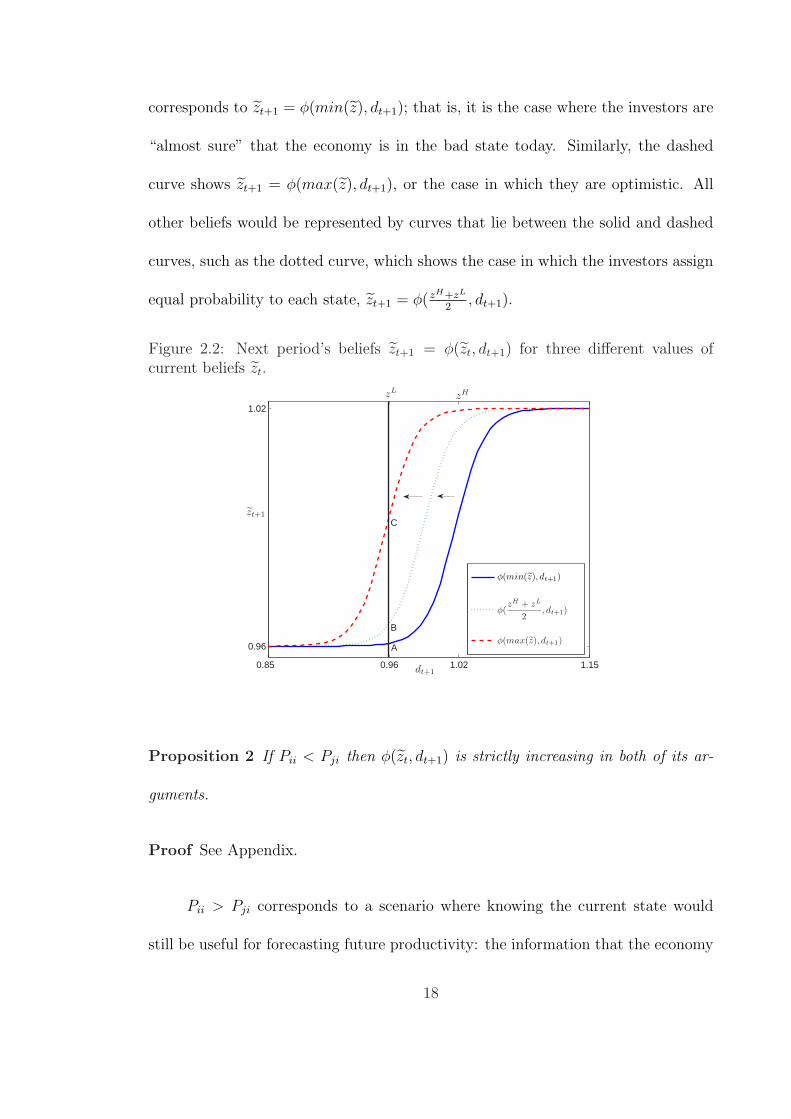
corresponds to zt+1 = φ(min(z), dt+1); that is, it is the case where the investors are

“almost sure” that the economy is in the bad state today. Similarly, the dashed

curve shows zt+1 = φ(max(z), dt+1), or the case in which they are optimistic. All

other beliefs would be represented by curves that lie between the solid and dashed

curves, such as the dotted curve, which shows the case in which the investors assign

equal probability to each state, zt+1 = φ( zH+zL

2, dt+1).

Figure 2.2: Next period’s beliefs zt+1 = φ(zt, dt+1) for three different values ofcurrent beliefs zt.

0.85 0.96 1.02 1.15

0.96

1.02

dt+1

zt+1

zLzH

φ(min(z), dt+1)

φ(zH + zL

2, dt+1)

φ(max(z), dt+1)A

B

C

Proposition 2 If Pii < Pji then φ(zt, dt+1) is strictly increasing in both of its ar-

guments.

Proof See Appendix.

Pii > Pji corresponds to a scenario where knowing the current state would

still be useful for forecasting future productivity: the information that the economy

18

is in a particular state would reveal that the economy is more likely to transition

to the other state than to stay in the same state in the subsequent period (negative

autocorrelation). Although information is valuable and learning would still take

place, we rule out the case Pii > Pji in order to establish Proposition 2.

The elasticity of zt+1 with respect to dt+1 varies depending on zt. When

the investors assign a high probability to being in the low state (zt is low), a low

realization of dt+1 “confirms” the beliefs and as a result zt+1 changes only marginally.

On the other hand, if a high dt+1 is observed, the beliefs of investors are “challenged”

and there is a large adjustment in the next period’s beliefs.

In order to see this, consider the following scenario. Assume that true produc-

tivity is low and that investors’ current beliefs are “almost correct”. In this case,

zt = min z, as depicted by “lowest beliefs” curve in Figure 2.2. The vertical line

in Figure 2.2 marks the mean of the signals conditional on the economy being in

the low state. Hence, a small negative noise shock is a realization of dividends to

the left of this vertical line. If investors observe a negative noisy signal at t + 1,

the response of beliefs to this signal is minimal (the solid curve is flat on the left

side of the vertical line). On the other hand, if investors receive a sequence of mis-

leading positive signals before the negative one, their optimism builds up and their

beliefs can move to reach that reflected in dashed curve in Figure 2.2. When the

economy ends up in this situation, the response to a small negative signal is large

(the dashed curve is steep on the left side of the vertical line). Therefore, a stream

of positive signals can move the economy to a vulnerable state in which a negative

signal triggers a large downward adjustment. As investors turn optimistic, it is as if

19

the economy is moving along the convex part of this curve. The point of maximum

vulnerability lies at the intersection of the vertical line and the inflection point of

the curve.

Figure 2.3 shows the numerical derivative of φ(zt, dt+1) with respect to dt+1

around dt+1 = zL as a function of zt.7 This derivative captures the response of

the beliefs to a small, negative signal conditional on true productivity being low,

and it approximates the “vulnerability” of the economy. Figure 2.3 illustrates that

this derivative is a convex function. Hence, the response of beliefs to a negative

signal increases at an increasing rate with the level of optimism attained prior to

the negative signal. The convexity of the derivative of φ(.) is due to the assumption

that true productivity is a discrete random variable. In the case of continuous

random variables, learning takes place in a linear fashion, that is, the posteriors are

a convex combination of the priors and the signal with weights that depend on the

signal-to-noise ratio. In that case, this derivative would be linearly increasing in the

level of optimism prior to the negative signal.

The quantitative analysis focuses on the model’s equilibrium which is defined

as follows.

Definition A competitive equilibrium is given by allocations α′(α, z, d), c(α, z, d),

α∗′(α, z, d) and asset prices q(α, z, d) such that:

(i) Domestic households maximize U subject to their budget constraint and their

information set, IU , taking asset prices as given.

7We approximate this derivative numerically with φ(z,zL)−φ(z,zL−ε)ε for ε small and positive. In

the figure, we plot this expression for different values of z.

20

Figure 2.3: The derivative of φ(zt, dt+1) with respect to dt+1 as a function of zt.

0.963 1 1.0280

0.4

0.8

1.2

ztzLzH

∂φ(zt, dt+1)

∂dt+1

(ii) Foreign investors maximize the expected present discounted value of future

profits conditional on their beliefs about the state of productivity, taking asset

prices as given.

(iii) The goods and asset markets clear.

21

Chapter 3

Quantitative Analysis

3.1 Computation

The dynamic programming representation of the domestic investors’ problem

for i, j ∈ {L,H} and i 6= j is:

V (α,z, d) = maxα′

{u(α(q + d)− α′q)

+ β[Pr(z = zi|IU)Pii + Pr(z = zj|IU)Pji

] ∫V (α′, φ(z, d′), d′)f(d′|z′ = zi)dd′

+ β[Pr(z = zi|IU)Pij + Pr(z = zj|IU)Pjj

] ∫V (α′, φ(z, d′), d′)f(d′|z′ = zj)dd′}.

(3.1)

The solution algorithm includes the following steps:

1. Discretize the state space. We use 102 equally spaced nodes for α and 40 equally

spaced nodes for z in the intervals [.83, 1.00] and [zL, zH ] respectively. To discretize

the noise component of dividends we use Gaussian quadratures with 20 quadrature

nodes.

2. Evaluate the evolution of beliefs zt+1 = φ(zt, dt+1) using Equations (2.13)-(2.16).

3. For a conjectured pricing function qold(α, z, d), solve the dynamic programming

problem described in Equation 3.1 using value function iterations in order to get

α′(α, z, d) and c(α, z, d).

22

4. Calculate the foreign investors’ demand function using domestic investors’ asset

demand function obtained in Step 3 and the market clearing condition in the asset

market, α∗ + α = 1.

5. Using foreign investors’ demand calculated in Equation (2.8), calculate new prices

qnew(α, z, d).

6. Update the conjectured prices with ξqold(α, z, d) + (1− ξ)qnew(α, z, d) where ξ is

a fixed relaxation parameter that satisfies ξ ∈ (0, 1) and is set close to 1 in order to

dampen hog cycles.

7. Iterate prices until convergence according to the stopping criterion max{|qnew −

qold|} < 0.00001 and get equilibrium asset prices q(α, z, d).

To check the accuracy of the solution of the dynamic programming problem,

we evaluate Euler equation residuals as described in Judd (1992). In order to do so,

we solve for c in the following Euler equation:

qtu′(ct) = βEt[(qt+1 + dt+1)u

′(ct+1)]. (3.2)

Intuitively, we evaluate the consumption function that exactly satisfies the Euler

equation implied by the solution of the dynamic programming problem. Then, we

calculate 1− (ct/ct), which is a unitless measure of error. We find that the average

Euler equation error is 0.0016.1

Euler equation errors do not include the errors from the price iteration since

the Euler equation must hold for any pricing function, not only the equilibrium

1Judd (1992) calls this measure the “bounded rationality measure,” and interprets an error of0.0016 as a $16 error made on a $10000 expenditure.

23

pricing function. As a measure for the accuracy of the equilibrium price, we report

the tolerance of the price iteration. Tolerance is defined as the maximum of the

absolute value of the difference between prices evaluated in the last two consecutive

iterations, max{|qnew − qold|}. We iterate prices until tolerance is less than 0.00001.

3.2 Calibration

The model is calibrated quarterly for Turkey using data for the 1987:1-2005:2

period. We set the risk free interest rate to average US Treasury Bill rate, R =

(1.0471).25 = 1.0115. We set β = 0.9886 and σ = 2 following the business cycles

literature. We set the trading costs of the foreign investors to {a = 0.001, θ = 0.1}.

With this calibration, total trading costs on average constitute 0.2589% of foreign

investors’ per period profits as specified in Equation (2.6) and 1.8845% of the trade

value. These costs are in line with the findings of Domowitz, Glen and Madhavan

(2001) showing equity trading costs during the period 1996-1998 for a total of 42

countries among which 20 are emerging countries. They found that for emerging

markets, trading costs are higher than the developed ones and they range between

0.58% (Brazil) and 1.97% (Korea) as percentage of trade value.

We estimate the parameters {ση, zH , zL} and Markov transition probabilities

{PHH , PLL} using a Maximum Likelihood Estimation procedure similar to the one

described in Hamilton (1989). For this exercise, we use quarterly GDP data for

Turkey from 1987:1 to 2005:2 with a total of 74 observations. The data are from

Central Bank of the Republic of Turkey’s web site and are in constant 1987 prices.

24

They are logged, seasonally adjusted (using the Bureau of Economic Analysis’s X12

Method) and filtered with HP filter using a smoothing parameter of 1600.

Table 3.1: Model parameters

β 0.9881 Discount factor

R 1.0121 Risk free rate

σ 2 Risk aversion coefficient

PHH 0.8933 Transition probability from H to H

PLL 0.6815 Transition probability from L to L

zL -0.0427 Productivity in state L

zH +0.0175 Productivity in state H

ση 0.0362 Standard deviation of noise

zH−zL

ση1.6638 Signal-to-noise ratio

{a, θ} {0.001, 0.1} Trading costs

We denote the observed GDP series as yt for t ∈ {1, 2, ..., T} and the pa-

rameters to be estimated are ψ ≡ {zi, zj, ση, Pii, Pjj}. The algorithm used for the

estimation is as follows:

1. Calculate the ergodic distribution of the Markov process, π = [πi πj], using

πi = (1− Pjj)/(2− Pjj − Pii). πj can be calculated using πi + πj = 1.

2. Calculate the conditional density:

f(yt, ψ|yt−1) =1√

2Πση

(Pr(zt = zi|yt−1)e

−(yt−zi)2

2σ2η + Pr(zt = zj|yt−1)e

−(yt−zj)2

2σ2η

)

(3.3)

where Pr(zt = zi|yt−1) denotes the posterior probability assigned to being in state

i conditional on the observed history of y until period t− 1.

25

3. For t = 1, when no history is available, use the ergodic probabilities calcu-

lated in Step 1 instead of the conditional probabilities.

4. Update the prior probability Pr(zt = zi|yt−1) using Bayesian updating

Equations 2.13 and 2.15.

5. Repeat Steps 2-4 for ∀t ∈ {1, 2, ..., T}.

6. The log likelihood function is evaluated by simply adding the logged con-

ditional density functions for all observations:

L(ψ) =T∑

t=1

ln f(yt; ψ|yt−1). (3.4)

7. Maximize the log likelihood function:

maxψ

L(ψ; yT ) (3.5)

subject to Pii > 0, Pjj > 0 and Pii > Pji (see Assumption).

The estimates of the productivity shock are {zH , zL} = {0.0175,−0.0427}

which translate into {exp(zH), exp(zL)} = {1 + 0.0177, 1− 0.0418}. The estimated

transition probabilities are PHH = 0.8933 and PLL = 0.6815. The estimated per-

sistent component variance is σz = 0.0260, and the estimated noise component

variance is ση is 0.0362, the ratio of the two is σz

ση= 0.7182. With these pa-

rameters, the estimated signal-to-noise ratio is zH−zL

ση= 1.6638. The productivity

shocks and the transition probability matrix approximate a Normal AR(1) process:

zt+1 = (0.0004) + (0.5763)zt + εt+1, where σε = 0.0213. This calibration implies

26

σε

ση= 0.5888 which constitutes another measure of information content of the sig-

nals.2

3.3 Quantitative Findings

Figure 3.1 shows the ergodic distribution of the domestic investors’ asset po-

sition, α, for a situation in which investors have full information (panel (a)) and

in which investors have incomplete information (panel (b)) scenarios. The “full in-

formation” scenario corresponds to the case in which the information set of both

investors is IIt ≡ {dt, dt−1, . . . , zt, zt−1, . . .}.3 In both cases, the ergodic distributions

are skewed to the left. The informational imperfection reduces the mean asset hold-

ings of domestic investors. This is because the informational imperfection increases

the uncertainty associated with future asset returns, and, hence, risk averse domestic

investors are less inclined to demand risky assets.

The ergodic distribution of beliefs, z, is plotted in Figure 3.2. In this distribu-

tion, most of the mass is concentrated at the tails, or around zL and zH . This result

arises because beliefs usually being close to correct. The extent to which the mass

is concentrated at the tails depends crucially on the signal-to-noise ratio. The more

informative the signals, the less beliefs deviate from the truth and the more the

ergodic distribution is concentrated at the tails. Another feature of this distribution

2This, in fact, is the conventional measure of the information content of the signals whenlearning takes place about continuous as opposed to discrete variables.

3One can model a full information scenario by setting ση = 0. However, doing so would alter thedistribution of the dividend process. As a result, it would not be possible to distinguish changesin results that are due to full information per se from those due to the change in the distributionof the dividend process.

27

Figure 3.1: Ergodic distribution of domestic investors’ asset holdings, α, in the caseof (a) full information, and (b) incomplete information.

0.82 0.88 0.94 1 α

(a)

1 0.940.880.82

(b)

α

Figure 3.2: Ergodic distribution of beliefs, z.

0.97 0.98 0.99 1 1.01zL zH Beliefs

is its skewness. Skewness is a result of the asymmetry of the Markov transition

matrix. The high state is more persistent than the low, an asymmetry that both

sets of investors acknowledge as they formulate their beliefs. Knowing that there

are more periods in which the economy is in the high state than in the low state,

investors’ beliefs are more likely to be close to zH than zL.

Table 3.2 documents the long run moments of simulated and actual data.4

Consistent with Figure 3.1, average asset holdings of the domestic investors is higher

4We simulate the model for 10,000 periods and calculate the moments after dropping the first1,000 observations.

28

Table 3.2: Long-run business cycle moments, simulated data is logged and HPfiltered.

Data Full Info. Incomplete Info.

E(d) 1.0036 1.0032

E(c) 0.8642 0.8419

E(α) 0.8609 0.8397

E(q) 83.1358 83.0617

E(CA/d) -0.0001 0.0001

σ(z) 2.5884 2.5884 2.5884

σ(η) 3.6341 3.6341 3.6341

σ(d) 4.5694 4.5514 4.5514

σ(c)/E(c) (%) 5.4597 2.1265 4.2168

σ(q)/E(q) (%) 38.0997 0.0370 0.0283

σ(CA/d) (%) 3.1168 3.6134 3.8935

corr(d, c) 0.6984 0.3153 0.4425

corr(d, q) 0.0718 0.5611 0.8327

corr(d, CA) -0.4217 0.9019 0.5801

corr(d, α′) 0.0347 0.1655

corr(z, z−1) x 0.5532

corr(z, q) 0.9990 0.6678

in the full information scenario than in the incomplete information scenario (86.1

percent v. 84 percent). As a result of their greater asset holdings, domestic investors’

consumption is also higher on average in the full information scenario than in the

incomplete information. In the full information case, higher average consumption

and lower consumption volatility lead to a higher level of welfare compared to the

case in which investors have only incomplete information.

29

Going from the full information setup to one with incomplete information,

the standard deviations of consumption and the current account increase by 2.1

percentage points, and 0.4 percent, respectively. On the other hand, the standard

deviation of asset prices falls by 0.87 basis points. The decline in the standard

deviation of asset prices is due to beliefs being a convex combination of the low and

high value of true productivity. (See Equation (2.16) and Proposition 1.)

The correlation between true productivity, z, and asset prices, q, falls from

0.9990 in the full information setup to 0.6678 in the incomplete information setup.

This is due to booms-busts induced by the imperfection of information, which gives

rise to misperceptions regarding the true state of productivity. In the full infor-

mation case, all of the cycles are driven by changes in true productivity and noise

shocks have negligible effects on asset prices. Although most of the booms and busts

in the incomplete information scenario are also due to changes in true productivity,

there is a significant number of optimism-pessimism driven cycles.

The autocorrelation coefficient of z is 0.5532 which suggests that transitory

shocks have persistent effects on beliefs. This occurs because investors cannot dis-

tinguish the component of shocks that is persistent from the component that is

transitory. The belief updating structure is the key element in the model that in-

duces persistence: the previous period’s posteriors are current period’s priors.

Another important observation from Table 3.2 is the decrease in the correlation

between dividends and the current account going from full information to imperfect

information (0.90 vs. 0.58). In response to a positive dividend shock, domestic

investors would like to increase their asset position so as to smooth consumption

30

over time and in addition, their expectations for asset returns increase since they

observe a positive signal. Foreign investors are modeled not to have a consumption

smoothing motive therefore, for them only the second effect (positive signal) is

present and this effect is in fact stronger than their domestic counterparts because

they bid more aggressively for the asset when there is a positive signal due to their

risk neutrality. Overall, we find that usually the first effect is greater than the

second, and therefore, the model produces a procyclical current account. However,

as we mentioned the procyclicality is lower compared to the full information scenario

where only the first effect is present.

Figure 3.3: Time series simulation for the case of full information.

−0.05

0

0.05z

−0.1

0

0.1η

−10

5x 10

−4 Price

−0.1

0.1Consumption

1 40 80−0.1

00.1

CA

Figures 3.3 and 3.4 show simulated asset prices, productivity, and consumption

31

Figure 3.4: Time series simulation for the case of incomplete information.

−0.05

0

0.05z

−0.1

0

0.1η

−10

5x 10

−4 Price

−0.1

0

0.1Consumption

1 40 80−0.1

0.1CA

32

under full information and incomplete information, respectively. In the full infor-

mation case, swings in asset prices match the swings in productivity and shocks

to the transitory component of dividends have minimal effects on prices. Without

the information role of dividends, in response to a negative noise shock domestic

investors would like to be net sellers so as to intertemporally smooth their con-

sumption and thus at equilibrium asset prices fall. However, this effect on prices

is small and not visible in the figure. In the incomplete information scenario, as-

set prices fluctuate both with true productivity and with transitory shocks. Noisy

signals thus can induce cycles driven by misperceptions among investors regarding

true productivity. In addition, as mentioned before, the volatility of consumption

increases substantially when we introduce informational imperfections.

In Figure 3.5, we plot the conditional forecasting functions starting from a

state where investors are optimistic (first column) and where they are pessimistic

(second column). In the optimistic scenario we set the state variables to (α, z, d) =

(0.840, 0.017, 0.958): that is, beliefs are z = max(z); dividends are set to signal

that the productivity is low; d = ezLand the domestic investors’ asset position

is set to its long-run mean. The pessimistic scenario is set to start at (α, z, d) =

(0.840,−0.042, 0.958). Hence, these scenarios are identical except for the initial

beliefs.

In the figures for consumption and asset prices, the vertical axes show per-

centage deviations from long-run means. In the figure for the current account, the

vertical axis shows the ratio of the current account to dividends in percentage terms.

On impact in period one, the economy with optimistic investors is characterized by a

33

Figure 3.5: Forecasting functions conditional on α = 0.840, d = zL, z = zH (firstcolumn), and z = zL (second column).

0 20 40 60 80 100−0.07

0

0.07 Price

0 20 40 60 80 100−2.5

0

1.5 Consumption

0 20 40 60 80 100−5.0

−2.5

0

2.5

5.0 Current Account

0 20 40 60 80 100−0.07

0

0.07Price

0 20 40 60 80 100−2.5

0

1.5 Consumption

0 20 40 60 80 100−5.0

−2.5

0

2.5

5.0 Current Account

34

current account deficit as well as a boom in consumption and asset prices. In period

two, however, consumption falls sharply below its mean by 1.5% and the current

account turns to a surplus of roughly 2.5%. The prices also adjust downwards but

the adjustment is more gradual than those of consumption and the current account.

After the second period, all variables slowly and monotonically converge to their

long-run means.

The dynamics of the model economy starting with optimistic investors are

similar to that of an emerging market in the period before a crisis. As documented in

Chapter 1, pre-crisis periods are generally characterized by current account deficits

as well as consumption and asset price booms. Our model is able to forecast a

collapse in consumption and asset prices as well as reversal of the current account

after this period of optimism.

The results in Table 3.2 suggested that the model produces a procyclical cur-

rent account on average and in the imperfect information scenario this procyclicality

is lower than in the full information case. Previously, we explained the model dynam-

ics that lead to this result. The forecasting functions plotted in Figure 3.5 support

the previous explanation and the results of Table 3.2. Particulary, the economy

with optimistic investors has a current account deficit because, ceteris paribus, the

higher the beliefs, the lower the current account.

Table 3.3 analyzes optimism and pessimism driven cycles in terms of their

frequency, average duration, and magnitude. In order to conduct the analysis, we

use simulated data to identify periods in which investors assign a probability greater

than 0.5 to productivity being high (low) even though the true productivity is low

35

Table 3.3: Analysis of optimism (pessimism) driven booms (busts).

Probability (%) Booms Busts

Prob[Prob(zt = zi|IUt , zt = zj) > 0.5] 9.6800 4.2300

Prob[Prob(zt = zi|IUt , zt = zj) > 0.5|zt = zj] 37.1023 5.7232

Duration (quarters)

Average duration 1.3552 1.2118

Magnitude (%)

q 0.0664 -0.0537

c 5.5420 -5.3174

CA 3.2158 -1.2994

Magnitude (in std. deviations)

q 2.3626 -1.9134

c 1.3143 -1.2764

CA 0.8320 -0.3362

(high) and call them optimism (pessimism) periods.5 In the second and third rows

of Table 3.3, we report the ratio of the number of optimism (pessimism) periods

to the total number of observations, and to the number of periods in which the

state was low (high), respectively. We calculate the average duration by calculating

the average length of the distinct optimism-pessimism periods. Given the inherent

noisiness of signals obtained by calibrating the model to a typical emerging economy,

this table reveals how often investors turn optimistic-pessimistic due to misleading

signals, how long these periods last, and more importantly, whether and how much

5Note that by doing so, we are picking up only those periods in which optimism and pessimismare due to misperceptions of investors.

36

optimism (pessimism) periods are associated with booms (busts) in asset prices and

consumption and current account deficits (surpluses).

Unconditionally, the model produces optimism driven booms with a 9.64%

probability, whereas it produces pessimism driven busts with a 4.23% probability.

Also, given that the true state is low, there is a 37.10% probability that the investors

are optimistic and similarly, conditional on the true productivity being high, the

investors are pessimistic with 5.72% probability. The former is more likely to happen

because investors interpret positive signals to be more “credible” than negative

signals due to the asymmetry of the Markov transition probability matrix. The

optimism in response to a misleading positive signal is greater than the pessimism

caused by a misleading negative signal with the same magnitude.

On average, the model predicts an average duration of 1.35 (1.21) quarters

for the optimism (pessimism) driven booms (busts). These cycles are relatively

short lived because these cycles hinge on the realization of a sequence of positive or

negative signals.

In the same table, we also report the size of these booms-busts as percentage

deviations from the value that corresponding variables would have taken if investors

had correctly estimated the true productivity instead of being optimistic or pes-

simistic. The magnitude for the asset price boom is small when we look at it as

percentage deviation because the equilibrium asset prices have low volatility. This

magnitude is closer to what we observe in the data in terms of standard deviations.

The boom periods are characterized by asset prices, consumption, and current ac-

count that are on average 2.36, 1.31, and 0.83 standard deviations above what they

37

would have been if the investors were not optimistic. The over-pricing as well as

over-consumption are evident in this table. Especially, the over-pricing of the emerg-

ing market asset is significant: during the booms on average we observe prices that

are more than two standard deviations higher that what they would have been if in-

vestors were not optimistic. Similarly, we see under-pricing and under-consumption

during the busts, although their magnitudes are smaller in absolute value than those

observed during booms due to the asymmetry of the Markov process.

3.4 From Miracles to Crises

In Figure 3.6 we plot the response of asset prices to a sequence of positive

signals, particularly to one, two, three and four consecutive one standard deviation

positive transitory shocks, respectively. In each of these scenarios, we set the true

state to low (z = zL) and with the one standard deviation transitory shocks, the

signals can be written as d = zL + ση. After the positive signals a truth revealing

signal (d = zL) arrives. Figure 3.6 plots the response of asset prices as percentage

deviations from its long run mean conditional on z = zL.

In line with the analysis of Chapter 2, Figure 3.6 establishes the relation

between the size of the booms and the magnitude of the downward adjustment due

to the truth revealing signal that arrives after the peak of the boom. Although

the signal that is observed after the positive signals is exactly the same in all of

these scenarios, asset prices respond differently because of learning dynamics, beliefs

respond more to challenging signals compared to the confirming ones.

38

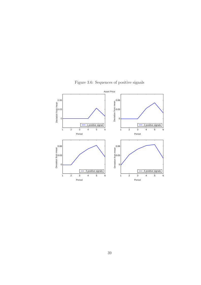
Figure 3.6: Sequences of positive signals

1 2 3 4 5 6

0

0.03

0.06

Period

Dev

iatio

n fr

om m

ean

1 2 3 4 5 6

0

0.03

0.06

Period

Dev

iatio

n fr

om m

ean

1 2 3 4 5 6

0

0.03

0.06

Period

Dev

iatio

n fr

om m

ean

1 2 3 4 5 6

0

0.03

0.06

Asset Price

Period

Dev

iatio

n fr

om m

ean

4 positive signals3 positive signals

2 positive signals1 positive signal

39

3.5 Turkey vs. U.S.

In order to establish the difference of a developed economy from a typical

emerging market economy, we estimate the model’s parameters governing the in-

formativeness of the signals using GDP data for the U.S. for the same time period

using the same estimation procedure.6 Not surprisingly, the total variance of the

U.S. GDP is significantly higher than that of Turkey (1.0121 vs. 4.5694).7 Table

3.4 reports the results of the estimation for the U.S. and also reproduces those for

Turkey. Comparing σ(z) and σ(η) for these two countries reveals that the variance

for the persistent component as well as the noise is lower for the U.S. In the model

at hand, the informativeness of signals is determined by the ratio of these two vari-

ances, or the signal-to-noise ratio. The signal-to-noise ratios estimated for the US

are zH−zL

ση= 2.7053 (vs. 1.6638 for Turkey) suggesting a more trivial learning for

the case of the U.S.

To see the differences of these two economies visually, we plot time series

simulations of the persistent and transitory shocks for the U.S. and Turkey in Figure

3.7, ensuring that the plots are in the same scale. In addition to the observations

made before, one can also see in this figure that for the case of Turkey, switches

between the low and high states of the persistent component are more frequent. This

is also consistent with the common argument that emerging market economies face

6U.S. data are from OECD’s web site, and are in constant prices, seasonally adjusted and HPfiltered with a smoothing parameter 1600.

7This volatility for the U.S. GDP is somewhat lower than the ones calculated by other studiesin the literature because we only consider the 1987:1-2005:2 period which is characterized by alower volatility compared the period before the 1980’s. We restrict our analysis to this time framesince quarterly Turkish data is available starting 1987.

40

Figure 3.7: Time series simulations for U.S. and Turkey.

−0.1

0.1U.S.

Dev

iatio

n fr

om tr

end

−0.1

0.1Turkey

Time

Dev

iatio

n fr

om tr

end

ηz

ηz

41

Table 3.4: U.S. vs Turkey, parameters

Turkey U.S.

PHH 0.8933 0.9117 Transition probability from H to H

PLL 0.6815 0.9317 Transition probability from L to L

zL -0.0427 -0.0054 Productivity in state L

zH 0.0175 0.0108 Productivity in state H

ση 0.0362 0.0060 Standard deviation of noise

zH−zL

ση1.6638 2.7053 Signal-to-noise ratio

σ(z) 2.5884 0.8109 Variance of the persistent component

σ(η) 3.6341 0.6124 Variance of the transitory component

σ(d) 4.5694 1.0121 Total variance

more frequent and dramatic changes in their fiscal and monetary policies potentially

due to higher political instability. Motivated by this striking difference in the signal-

to-noise ratios of these economies, we solve our model with the U.S. calibration,

analyze its implications and report the results in Table 3.5.

Table 3.5 documents the magnitude, frequency and the duration of booms and

busts due to misperceptions of investors for the cases of U.S. and Turkey. Definitions

of optimism and pessimism and all of the calculations are the same as those of Table

3.3. The first two rows of the table reveal that the unconditional and conditional

probabilities of both booms and busts are lower for the case of U.S. compared to

Turkey. This is mainly driven by the higher signal-to-noise ratio estimated for the

U.S. leading to more informative signals and making it less likely for the investors

to be misled. Another observation is the reversed asymmetry, for Turkey optimism

42

Table 3.5: U.S. vs Turkey, booms and busts

Turkey U.S.

Probability (%) Booms/Busts Booms/Busts

Prob[Prob(zt = zi|IUt , zt = zj) > 0.5] 9.6800/4.2300 1.7836/2.4004

Prob[Prob(zt = zi|IUt , zt = zj) > 0.5|zt = zj] 37.1023/5.7232 3.1388/4.5598

Duration (quarters)

Average duration 1.3552/1.2118 1.1383/1.1163

Magnitude (%)

q 0.0664/-0.0537 0.0724/-0.0633

c 5.5420/-5.3174 1.1825/-0.8576

CA 3.2158/-1.2994 1.8730/-1.0329

Magnitude (in std. deviations)

q 2.3626/-1.9134 1.5894/-1.3924

c 1.3143/-1.2764 1.1498/-0.8475

CA 0.8320/-0.3362 0.5062/-0.2792

driven booms occur with a higher probability than busts whereas pessimism driven

busts are more likely for the U.S. A careful observation of Table 3.4 reveals that the

low state is slightly more persistent than the high state (comparing PLL with PHH)

for the U.S. which is in contrast with the case of Turkey. This difference in the

Markov transition matrices estimated for these countries accounts for the reversed

asymmetry.

In terms of the durations, the cycles generated by the model calibrated Turkey

are on average longer than those generated by the model calibrated to the U.S.

43

Noisier signals for the case of Turkey make it more likely for the investors to receive

consecutive misleading signals and extend the time it takes for them to correct their

beliefs leading to longer misperceptions driven booms and busts.

The magnitude of consumption booms/busts are significantly larger for Turkey

than the U.S. but this result does not hold for asset prices. The higher signal-to-

noise ratio for the U.S. leads to a higher asset price volatility.8 In units of the

standard deviations of the corresponding variables reported in the last three rows,

all of the magnitudes are larger for the case of Turkey.

3.6 Sensitivity Analysis

We document the long run business cycle moments of the model with different

calibrations for the noisiness of the signals, ση, and trading costs, a and θ. The third

column of Table 3.6 shows the results with ση = 0.0265 and we compare these results

with those of the baseline model with ση = 0.0362 reproduced in the second column.9

With lower ση, the standard deviation of dividends, consumption and the current

account fall by 85, 20, and 27 basis points, respectively. Average consumption

among domestic investors increases due to the lower volatility of dividends and the

associated decrease in uncertainty regarding future asset returns.

Lower ση implies that the signals are more informative and credible. Therefore,

learning is faster compared to the baseline scenario. This leads to less persistence in

beliefs. The autocorrelation of beliefs drops down to 0.54 from 0.55 in the baseline

8Remember that the full information model produces more volatile asset prices than the incom-plete information as documented in Table 3.2.

9With ση = 0.0265 the signal-to-noise ratio increases to 2.26 from 1.66 in the baseline scenario.

44

Table 3.6: Sensitivity analysis, simulated data is logged and linearly detrended.

Incomplete Information Baseline ση = 0.0265 a = 0.002 θ = 0

E(d) 1.0036 1.0036 1.0036 1.0036

E(c) 0.8419 0.8472 0.8663 0.8417

E(q) 83.0617 83.0937 82.9521 83.0636

E(α) 0.8397 0.8448 0.8637 0.8398

E(CA) 0.0001 0.0001 -0.0001 -0.0001

σ(z) 2.5884 2.5884 2.5884 2.5884

σ(η) 3.6341 2.6512 3.6341 3.6341

σ(d) 4.5514 3.6997 4.5514 4.5514

σ(c)/E(c) (%) 4.2168 4.0287 4.4765 4.2153

σ(q)/E(q) (%) 0.0283 0.0291 0.0288 0.0285

σ(CA) (%) 3.8935 3.7166 4.5698 3.8472

corr(d, c) 0.4425 0.4318 0.2163 0.4519

corr(d, q) 0.8327 0.8505 0.8038 0.8313

corr(d, α′) 0.1655 0.1403 0.0216 0.2064

corr(d, CA) 0.5801 0.6032 0.6591 0.5751

corr(z, z−1) 0.5532 0.5407 0.5532 0.5532

corr(z, q) 0.6678 0.7282 0.6694 0.6761

model. In addition, the probability of optimism-pessimism driven cycles falls leading

to a stronger correlation between asset prices and true productivity.

The fourth column of the same table presents the results for the scenario with

higher per trade costs, a = 0.002. The standard deviation of prices, consumption,

and the current account increase by 0.05, 26, and 67 basis points, respectively. Due

to higher per trade costs on the foreign investors’ side, domestic investors hold more

45

of the asset in equilibrium, leading to higher mean consumption but more volatile

consumption.

Analysis of the scenario with no recurrent costs, θ = 0, is reported in the fifth

column. The results remain largely unchanged except for the slight drops in the

current account volatility and the correlation of the current account with dividends.

46

Chapter 4

Asymmetric Information

In this section we modify the baseline incomplete information model by as-

suming that domestic investors observe the true state of productivity but that the

signal extraction problem facing the foreign investors’ remains identical to that in

the previous section. The aim of this exercise is to investigate whether the results

for the incomplete information case hinge on the informational homogeneity of in-

vestors (i.e., on whether the results change when the investors are asymmetrically

informed and they “disagree” on the state of the economy.)

The information set of domestic investors as of time t, IIt , is now defined as:

IIt ≡ {dt, dt−1, . . . , zt, zt−1, . . .}. (4.1)

The foreign investors’ information set is a subset of domestic investors’, IU ⊂ II

for ∀ t.1 Domestic investors maximize the same objective function as before, but

conditional on the information set in Equation (4.1)subject to Equation (2.2) and

taking the evolution of foreign investors’ beliefs, z′ = φ(z, d′), as given. Even though

they are fully informed, domestic investors keep track of foreign investors’ beliefs,

as they contain information useful for predicting future asset prices.

1Since the information sets of investors can be hierarchically ranked, we do not face an “infiniteregress problem”; i.e., agents do not forecast the forecasts of other agents, avoiding an infinitelydimensional belief space.

47

The objective function and belief updating process of the foreign investors

are the same as in the previous setup. Contrary to conventional models in which

prices reveal information, we abstract from the informational role of prices. This

assumption is implicit in the belief updating equations, where the only signals con-

sidered are the realizations of dividends. One justification for this assumption is

that, as long as prices are not fully revealing, which is likely to be the case even in

developed country asset markets, asset prices will be sensitive to the misperceptions

of uninformed investors. Wang (1994) shows that this is the case using a model

with asymmetric information. In Wang’s model, the equilibrium price has an in-

formational role and is a linear function2 of the return from the private investment

opportunity, the persistent component of dividends (which is what the uninformed

wish to know about), and the uninformed investors’ beliefs. When prices are par-

tially revealing, they act as a device that transmits information from the informed

to the uninformed, lowering the informational gap between the two. In a model in

which prices do not play any informational role, this gap will be larger compared

to an identical model in which prices reveal information. Our strategy to deal with

this problem is to calibrate the model so that dividends are ‘very’ informative and

reveal sufficient information to prevent the informational gap from becoming too

large.

There are two uncertainties faced by domestic households in this setup: the

evolution of the true productivity (which enters the problem directly) and the be-

liefs of foreign investors (which enters indirectly). The latter enters the domestic

2The model is solved analytically assuming CARA utility and Normally distributed returns.

48

investors’ problem since the introduction of imperfect information to the foreign

investors’ problem has implications for the domestic investors’ problem as well. The

beliefs of foreign investors affect asset prices and are persistent. They contain infor-

mation for forecasting next period’s prices. Domestic investors treat these beliefs as

a state variable and form expectations about the following period’s beliefs. However,

due to their advantage in separating persistent shocks from noise, on average their

forecasts of future beliefs are more accurate than those of their foreign counterparts’.

Mathematically,

Proposition 3 {E [E[zt+1|II

t ]− zt+1

]}2 < {E [E[zt+1|IU

t ]− zt+1

]}2.

Proof See Appendix.

4.1 Quantitative Analysis

With asymmetric information, the total dividend is not a sufficient state vari-

able; z and η enter as separate state variables. The dynamic programming repre-

sentation of the domestic households’ problem is:

V (α, z, η, z) = maxα′,c

u(c) + βE[V (α′, z′, η, z′|I i)] (4.2)

subject to

c + α′q(α, z, η, z) = αq(α, z, η, z) + αd (4.3)

and

z′ = φ(z, d′) (4.4)

49

for given prices q(α, z, η, z). In order to solve the problem numerically, we substitute

for consumption using the budget constraint, substitute for z′ using the evolution

of beliefs, and rewrite the problem as follows for i, j ∈ {H, L} and i 6= j:

V (α, z, η, zi) = maxα′

u(αq(α, z, η, z) + αd− α′q(α, z, η, z))+

βPii

∫V (α′, φ(z, d′), η′, zi)f(d′|zi)dd′+

βPij

∫V (α′, φ(z, d′), η′, zj)f(d′|zj)dd′.

(4.5)

Table 4.1 documents the long run moments of the simulated data. The third

column shows the results for the asymmetric information scenario, whereas the

second column repeats the results of the incomplete information case for comparison.

The most significant difference in the long run moments of these two setups is the

current account volatility and its correlation with dividends. The standard devation

of the current account increases by 7% and its correlation with dividends drops from

0.58 in incomplete information scenario to -0.40 in the asymmetric information case.

This findings suggests that the asymmetric information setup leads to more frequent

trade and higher trading volume because agents trade not only due to differences in

their objective functions but also due to differences in their perceptions of the current

state and in their expectations regarding future returns. Unlike in the incomplete

information setting, domestic investors in the asymmetric information setup can

make capital gains by better predicting the following period’s prices. Indeed, they

have an incentive to “run against the wind” to make capital gains.

Being able distinguish the transitory shocks from the permanent makes asset

50

Table 4.1: Simulations for the asymmetric information setup; simulated data arelogged and linearly detrended.

Incomplete Information Asymmetric Information

E(d) 1.0032 1.0032

E(c) 0.8419 0.8503

E(q) 83.0617 83.0609

E(α) 0.8397 0.8481

E(CA) 0.0001 0.0001

σ(z) 2.5884 2.5884

σ(η) 3.6341 3.6341

σ(d) 4.5514 4.5514

σ(c)/E(c) (%) 4.2168 4.2227

σ(q)/E(q) (%) 0.0283 0.0285

σ(CA/d) (%) 3.8935 11.9711

corr(d, c) 0.4425 0.2505

corr(d, q) 0.8327 0.8322

corr(d, α′) 0.1655 0.0513

corr(d, CA) 0.5801 -0.4018

corr(z, z−1) 0.5532 0.5532

corr(z, q) 0.6678 0.5681

investment less risky for domestic investors. On average, domestic investors demand

more of the asset. In response to a positive transitory component shock, the domestic

investors would like to buy more of the asset in order to smooth consumption. Their

incentives to increase asset holdings are stronger than under incomplete information

since they do not face the risk of being misled by a noisy signal. Hence, on average,

their demand for the asset is higher.

51

Domestic investors’ asset demand decision is affected through two channels in

response to transitory shocks. First, negative (positive) transitory shocks imply low

(high) dividends and hence the domestic investors would like to become net sellers

(buyers) of the asset in order to smooth their consumption over time. This lowers

(increases) the demand of domestic investors, and it is present in the full information

case as well.

The second effect arises due to the capital gain opportunity for domestic in-

vestors who have an informational advantage over their foreign counterparts. When

the asset is undervalued (overvalued) due to the misperceptions of foreign investors,

domestic investors know that this is the result of a transitory shock, and that prices

will eventually correct. As a result, they would like to use the opportunity to buy

(sell) the asset when the prices are low (high) due to the pessimism (optimism) of

foreign investors. We find that on average the capital gain opportunity dominates

the consumption smoothing effect and we find a negative correlation between the

current account and dividends.

52

Chapter 5

Conclusion

The boom-bust cycles of emerging economies suggest that periods of apparent

prosperity in these countries might contain the seeds of crises. This thesis explores

this possibility using an open economy equilibrium asset pricing model with im-

perfect information in which agents do not know the true state of productivity in

the economy. The model proposed in this thesis can endogeously generate periods

of optimism characterized by booms in asset prices and consumption followed by

sudden reversals, and sensitivity to negative signals that increases with, and arises

from, investor optimism attained prior to the negative signal. These results are due

to the fact that informational frictions generate a disconnect between country fun-

damentals and asset prices. That is, busts (booms) in asset markets can occur even

though the fundamentals of the economy are strong (weak). Asset prices display

persistence in response to transitory shocks since investors cannot perfectly iden-

tify the underlying state of productivity. Due to the additional uncertainty created

by informational frictions, the volatility of the emerging economy’s consumption

increases by 2 percentage points compared to the full information scenario. In ad-

dition, periods with high levels of optimism are more likely to be associated with

current account deficits than periods of pessimism.

In addition, this thesis quantifies the signal-to-noise ratios of a typical emerg-

53

ing market economy and a developed economy and establishes that informational

frictions are more prevalent for emerging markets. Based on this difference, we

show that emerging markets are more likely to experience booms and busts due to

misperceptions of investors. Also, these cycles tend to last longer and have larger

magnitudes compared to those of the U.S.

Although the informational frictions introduced in this thesis can produce

booms and busts in asset prices and consumption due to shifts in investor confidence,

these booms and busts are short lived and are of about the same size as regular

business cycles. In addition, even though the introduction of imperfect information

provides an improvement in terms of matching the volatility of consumption and

the current account dynamics observed in the data, the model cannot account for

the volatility of asset prices.

The role of informational frictions in understanding emerging market regu-

larities is an area ready for further research. For instance, the model presented in

this thesis endogenously produces sensitivity to negative signals given an exogenous

sequence of positive signals. We could think of producing an endogeous sequence of

positive signals by introducing strategic information manipulation into the model,

especially prevalent during the run-ups to crises. If there is initially some sensitiv-

ity due to short-term and/or dollarized debt, a policymaker might find it optimal

to manipulate or screen the signals to send positive signals. However, this would

come at a cost because, by taking out the negative signals and sending only posi-

tive ones, the sensitivity of the economy to a sudden downward adjustment would

increase. This would create a feedback mechanism in which the policymaker, con-

54

cerned about the country’s ability to continue borrowing in international markets,

has a self-perpetuating incentive to hide negative information about the economy

from the public.

55

Appendix A

Proofs

Throughout this section, we assume that i, j ∈ {L,H} and i 6= j.

Proof of Proposition 1

Denote the prior Pr(zt = zi|Iut−1) = pt(i) and the Normal density function

f(dt|zt = zi) = f(i) for i ∈ {L,H}.

Priors:

Evolution of pt(i) is characterized by:

pt(i) =pt−1(i)f(i)Pii + [1− pt−1(i)]f(j)Pji

pt−1(i)f(i) + [1− pt−1(i)]f(j).

• pt(i) = 1 ⇔ pt−1(i)f(i)Pii +[1−pt−1(i)]f(j)Pji = pt−1(i)f(i)+[1−pt−1(i)]f(j)

and pt−1(i)f(i) + [1− pt−1(i)]f(j) 6= 0. Given P >> 0 (see Assumption), the

first condition is satisfied iff

pt−1(i) = 0 and f(j) = 0 or

pt−1(i) = 1 and f(i) = 0, both of which violate the second condition.

• pt(i) = 0 ⇔ f(j)Pji + pt−1(i)[f(i)Pii − f(j)Pji] = 0 and pt−1(i)f(i) + [1 −

pt−1(i)]f(j) 6= 0. The first condition is satisfied iff

f(j) = 0 and f(i)Pii = f(j)Pji. These two hold iff f(j) = 0 and f(i) = 0,

in which case the second condition above does not hold.

56

f(j) = 0 and pt−1 = 0. In this case, second condition is again violated.

See Liptser and Shiryayev (1977) Ch. 9 and David (1997) for the proof of entrance

boundaries in continuous time.

Posteriors:

Rewrite Equation (2.13):

Pr(zt = zi|IUt ) =

pt−1(i)f(i)

pt−1(i)f(i) + [1− pt−1(i)]f(j).

Clearly, all terms on the right hand side of the equation are positive: p > 0 (the

proof above) and f > 0 (Normal distribution).

Proof of Proposition 2

First Argument: We need to show that ∂φ(zt,.)∂zt

> 0 for ∀ zt. Denote the

posterior probabilities Pr(zt = zi|IUt ) = γt and f(dt+1|zt = zi) = f(i). We start

with expressing γt+1 as a function of γt:

γt+1 =[γtPii + (1− γt)Pji]f(i)

[γtPii + (1− γt)Pji]f(i) + [1− γtPii − (1− γt)Pji]f(j). (A-1)

Also:

∂φ(zt, dt+1)

∂zt

=∂zt+1

∂zt

=∂zt+1

∂γt+1

∂γt+1

∂γt

∂γt

∂zt

. (A-2)

Remember that zt = γtzi + (1 − γt)z

j, so we can calculate the first and the third

57

expressions in the above equation:

∂zt+1

∂γt+1

= zi − zj,∂γt

∂zt

=1

zi − zj. (A-3)

The second expression can be calculated using Equation (A-1). After some manip-

ulation:

∂γt+1

γt

=f(zi)f(zj)(Pii − Pji)

{[γtPii + (1− γt)Pji]f(i) + [1− γtPii − (1− γt)Pji]f(j)}2. (A-4)

Plug in Equations (A-3) and (A-4) into Equation (A-2). To complete the proof, we

need to establish f(zi), f(zj) > 0 and Pii > Pji. f(zi), f(zj) > 0 for ∀zi, zj since the

Normal distribution is unbounded. Pii > Pji follows from Assumption 2.3.

Second Argument: We need to show that ∂φ(.,dt+1)∂dt+1

> 0. Write:

∂φ(., dt+1)

∂dt+1

=∂zt+1

∂dt+1

=∂zt+1

∂γt+1

∂γt+1

∂dt+1

. (A-5)

Denote A = Pij + γ(Pii − Pji). Then we can rewrite Equation (A-1):

γt+1 =Af(i)

Af(i) + (1− A)f(j)=

1

1 + 1−AA

f(j)f(i)

. (A-6)

Write f(i) and f(j) explicitly:

f(j)

f(i)= e

12σ2 [(dt+1−zi)2−(dt+1−zj)2] = e

(2dt+1−zj−zi)(zj−zi)

2σ2 .

58

Then we can calculate its derivative with respect to dt+1:

∂[f(j)/f(i)]

∂dt+1

=zj − zi

σ2e

(2dt+1−zj−zi)(zj−zi)

2σ2 . (A-7)

Rewrite Equation (A-5):

∂zt+1

∂dt+1

=∂zt+1

∂γt+1

∂γt+1

∂[f(j)/f(i)]

∂[f(j)/f(i)]

∂dt+1

. (A-8)

We know the first expression from Equation (A-2). The second expression can be

calculated using Equation (A-6):

∂γt+1

∂[f(j)/f(i)]=

−(1− A)/A

(1 + [(1− A)/A][f(j)/f(i)])2 . (A-9)

Plugging in Equations (A-2), (A-7) and (A-9) into (A-8) and rearranging we get:

∂zt+1

∂dt+1

=

[zi − zj

σ[1 + (1− A)/A(f(j)/f(i))]

]2

e(2dt+1−zj−zi)(zj−zi)

2σ2 > 0.

Proof of Proposition 3

Assume zt = zi without loss of generality. Write:

E[zt+1|IIt ] = E[φ(zt, dt+1)|II

t ] = Pii

∫φ(zt, z

i +η)dη+Pij

∫φ(zt, z

j +η)dη. (A-10)

Since IIt includes the history of all variables as well as the distributions govern-

ing them, and since the informed agents use their information rationally, we have

59

E[zt+1|IIt ] = E[zt+1]. This implies {E[E[zt+1|II

t ] − zt+1]}2 = 0. To complete the

proof, we need to show that {E[E[zt+1|IUt ]− zt+1]}2 > 0. Write

{E[E[zt+1|IUt ]− zt+1]}2 = {E[E[zt+1|IU

t ]|IIt ]− E[zt+1|II

t ]}2.

And write the expression for E[zt+1|IUt ] denoting posterior probabilities Pr(zt =

zi|IUt ) = γt:

E[zt+1|IUt ] = [γtPii+(1−γt)Pji]

∫φ(zt, z

i+η)dη+[γtPij+(1−γt)Pjj]

∫φ(zt, z

j+η)dη

(A-11)

Combine Equation (A-10), Equation (A-11), and Pij = 1− Pii to write:

{E[zt+1|IUt ]−E[zt+1|II

t ]}2 = (1−γt)2(Pii+Pjj−1)2[

∫φ(zt, z

j+η)dη−∫

φ(zt, zi+η)dη]2

Clearly, {E[zt+1|IUt ]− E[zt+1|II

t ]}2 ≥ 0 with equality iff

• γt = 1 or

• Pjj = Pij or

• φ(zt, zi + η) = φ(zt, z

j + η)

Proposition 1 establishes that γ ∈ (0, 1), which rules out condition 1. Condition

2 does not hold by assumption (see text). Finally, condition 3 is violated because

zL 6= zH (see text) and φ(., .) is monotonically increasing in its second argument.

60

BIBLIOGRAPHY

[1] Aguiar, Mark and Gita Gopinath, 2004, “Emerging Market Business Cycles:

The Cycle is the Trend,” under review.

[2] Aiyagari, S. Rao and Mark Gertler, 1999, “ ‘Overreaction’ of Asset Prices in

General Equilibrium,” Review of Economic Dynamics, vol.2, issue 1, pp.3-35.

[3] Albuquerque, Rui, Gregory H. Bauer, and Martin Schneider, 2004, “Interna-

tional Equity Flows and Returns: A Quantitative Equilibrium Approach,” un-

der review at The Review of Economic Studies.

[4] Andersen, Torben M. and Niels C. Beier, 2005, “International Transmission

of Transitory and Persistent Monetary Shocks Under Imperfect Information,”

Journal of International Economics, Article in press.

[5] Caballero, Ricardo J. and Arvind Krishnamurthy, 2001, “International and Do-

mestic Collateral Constraints in a Model of Emerging Market Crises,” Journal

of Monetary Economics, 48, pp. 513-548.

[6] Calvo, Guillermo, 1999, “Contagion in Emerging Markets: When Wall Street is

a Carrier,” proceedings from the International Economic Association Congress,

vol.3.

[7] Calvo, Guillermo and Carmen Reinhart, 2000, “When Capital Inflows Come to

a Sudden Stop: Consequences and Policy Options,” Key Issues in Reform of the

International Monetary and Financial System by Peter Kenen and Alexandre

Swobod, International Monetary Fund, 175-201.

61

[8] Calvo, Guillermo and Enrique Mendoza, 2000, “Rational Contagion and the

Globalization of Securities Markets,” Journal of International Economics, Vol.

51, 79-114.

[9] Chakravarty, Sugato, Asani Sarkar, and Lifan Wu, 1998, “Information Asym-

metry, Market Segmentation, and the Pricing of Cross-listed shares: Theory

and Evidence From Chinese A and B Shares,” Federal Reserve Bank of New

York, Research paper, 9820.

[10] Chan, K.A., A.J. Menkveld, and Z. Yang, 2003, “Evidence on the Foreign Share

Discount Puzzle in China: Liquidity or Information Asymmetry?,” Working

paper.

[11] Choe, Hyuk, Bong-Chan Kho and Rene M. Stulz, 2001, “Do Domestic Investors

Have More Valuable Information About Individual Stocks Than Foreign In-

vestors?,” Working paper, NBER, 8073.

[12] Chui, A. and C. Kwok, 1998, “Cross-autocorrelation Between A Shares and

B Shares in the Chinese Stock Market,” Journal of Financial Research, 21,

333-353.

[13] Corbett, Jenny, Gregor Irwin and David Vines, 1999, “From Asian Miracle

to Asian Crisis: Why Vulnerability, Why Collapse?,” presented at the confer-

ence titled “Capital Flows and the International Financial System,” Australian

Central Bank.

62

[14] David, Alexander, 1997, “Fluctuating Confidence in Stock Markets: Implica-

tions for Return and Volatility,” Journal of Financial and Quantitative Analy-

sis, vol. 32, no. 4.

[15] Domowitz, Ian, Jack Glen and Ananth Madhavan, 2001, “Liquidity, Volatil-

ity, and Equity Trading Costs Across Countries and Over Time,”International

Finance, vol. 4, issue 2, pp.221.

[16] Dvorak, Tomas, 2001, “Do Domestic Investors Have an Information Advan-

tage? Evidence from Indonesia,” Working paper, Williams College, Center for

Development Economics, 168.

[17] Frankel, Jeffrey A. and Sergio L. Schmukler, 1996, “Country Fund Discounts

and The Mexican Crisis of December 1994: Did Local Residents Turn Pes-

simistic Before International Investors?,” Board of Governers of the Federal

Reserve System, International Finance Dicussion Papers #563.

[18] Furman, Jason and Joseph E. Stiglitz, 1998, “Economic Crisis: Evidence and

Insights from East Asia,” Brookings Papers on Economic Policy, #2, pp. 1-114.

[19] Gourinchas, Pierre-Olivier and Aaron Tornell, 2003, “Exchange Rate Dynam-

ics, Learning and Misperception” CEPR Discussion Papers 3725, C.E.P.R. Dis-

cussion Papers.

[20] Grinblatt, Mark and Matti Keloharju, 2000, “The Investment Behavior and

Performance of Various Investor Types: A Study of Finland’s Unique Data

Set,” Journal of Financial Economics, 55(1), 43-67.

63

[21] Hau, H., 2001, “Location Matters: An Examination of Trading Profits,” Jour-

nal of Finance, 56, No. 5, pp. 1959-1983.

[22] Hamilton, James D., 1989, “A New Approach to the Economic Analysis of

Non-stationary Time Series and the Business Cycle ,” Econometrica, 57, pp.

357-384.

[23] Heaton, John and Deborah J. Lucas, 1996, “Evaluating the Effects of Incom-

plete Markets on Risk Sharing and Asset Pricing,” Journal of Political Econ-

omy, 104, 3, pp. 443-487.

[24] IMF World Economic Outlook, May 1998.

[25] IMF Survey Supplement on the Fund, September 2001.

[26] Judd, Kenneth L., 1992, “Projection Methods for Solving Aggregate Growth

Models,” Journal of Economic Theory, 58, pp. 410-452.

[27] Kang, Jun-Koo and Rene M. Stulz, 1997, “Why is there a home bias? An

Analysis of Foreign Portfolio Equity Ownership in Japan,” Journal of Financial

Economics, 46, 2-28.

[28] Liptser, Robert S. and Albert N. Shiryaev, 1974, “Statistics of Random Pro-

cesses I General Theory,” Springer- Verlag Berlin Heiderberg.

[29] Masson, Paul R., 1999, “Multiple Equilibria, Contagion and the Emerging Mar-

ket Crises,” IMF Working paper 99/164.

64

[30] Mendoza, Enrique, G., 1991, “Real Business Cycles in a Small Open Economy,”

American Economic Review, 81, pp. 797-818.

[31] Mendoza, Enrique, G. and Katherine A. Smith, 2004, “Quantitative Implica-

tions of a Debt-Deflation Theory of Sudden Stops and Asset Prices,” Working

paper, NBER, 10940.

[32] Moore, Bartholomew and Huntley Schaller, 2002, “Persistent and Transitory

Shocks, Learning and Investment Dynamics,” Journal of Money, Credit and

Banking, vol. 34, no. 3, pp. 650-677.

[33] Morris, Stephen and Hyun Song Shin, 1998, “Unique Equilibrium in a Model

of Self-Fulfilling Currency Attacks,” American Economic Review, vol. 88, no.

3, pp. 587-597.

[34] Nieuwerburgh, Stijn and Laura Veldkamp, 2004, “Learning Asymmetries in

Real Business Cycles,” conditionally accepted at Journal of Monetary Eco-

nomics.

[35] Paasche, Bernhard, 2001, “Credit Constraints and International Financial

Crises,” Journal of Monetary Economics, 28, pp.623-650.

[36] Seasholes, Mark, 2000, “Smart Foreign Traders in Emerging Markets,” Working

paper, Harvard Business School, Cambridge, MA.

[37] Wang, J., 1994, “A Model of Competitive Stock Trading Volume,” Journal of

Political Economy, 102: 127168.

65