2, boulevard RoyalL-2983 Luxembourg

Tél. : +352 4774-1Fax: +352 4774 4910

www.bcl.lu • info@bcl.lu

CAHIER D’ÉTUDES WORKING PAPER

N° 116

CHAINED FINANCIAL FRICTIONS AND CREDIT CYCLES

FEDERICO LUBELLO IVAN PETRELLA EMILIANO SANTORO

FEBRUARY 2018

Chained Financial Frictions and Credit Cycles∗

Federico Lubello† Ivan Petrella‡ Emiliano Santoro§

February 2, 2018

Abstract

We examine the role of bank collateral in shaping credit cycles. To this end, we develop

a tractable model where bankers intermediate funds between savers and borrowers. If bankers

default, savers acquire the right to liquidate bankers’ assets. However, due to the vertically

integrated structure of our credit economy, savers anticipate that liquidating financial assets

(i.e., bank loans) is conditional on borrowers being solvent on their debt obligations. This

friction limits the collateralization of bankers’ financial assets beyond that of other assets that

are not involved in more than one layer of financial contracting. In this context, increasing

the pledgeability of financial assets eases more credit and reduces the spread between the loan

and the deposit rate, thus attenuating capital misallocation as it typically emerges in credit

economies a la Kiyotaki and Moore (1997). We uncover a close connection between the collater-

alization of bank loans, macroeconomic amplification of shocks and the degree of procyclicality

of bank leverage. A regulator may reduce macroeconomic volatility through the introduction

of a countercyclical capital buffer, while a fixed capital adequacy requirement displays limited

stabilization power.

JEL classification: E32, E44, G21, G28.

Keywords: Banking; Bank Collateral; Liquidity; Capital Misallocation; Macroprudential Policy.

∗We thank—without implicating—Martin Gonzalez Eiras, Omar Rachedi, Søren Hove Ravn, Raffaele Rossi,Abdelaziz Rouabah, and participants at the “2017 Computation in Economics and Finance Conference” at FordhamUniversity in New York for helpful comments and suggestions. Part of this work has been conducted while Santorowas visiting Banco de Espana, whose hospitality is gratefully acknowledged. This paper should not be reported asrepresenting the views of the Banque centrale du Luxembourg (BcL) or the Eurosystem. The views expressed arethose of the authors and may not be shared by other research staff or policymakers in the BcL or the Eurosystem.†Banque centrale du Luxembourg. Address: 2, Boulevard Royal, L-2983 Luxembourg. E-mail :

federico.lubello@bcl.lu.‡Warwick Business School and CEPR. Address: Warwick Business School, The University of Warwick, Coventry,

CV4 7AL, UK. E-mail : Ivan.Petrella@wbs.ac.uk.§Department of Economics, University of Copenhagen. Address: Østerfarimagsgade 5, Building 26, 1353 Copen-

hagen, Denmark. E-mail : emiliano.santoro@econ.ku.dk.

1

Non-technical summary

Financial institutions resort to collateralized debt to raise funds, providing assets as a guarantee

in case of default on their debt obligations. This is the case for non-traditional banking activities

with sale and repurchase agreements (repos) employed as a main source of funding. It is also true

for commercial banks, which employ financial collateral both for currency management purposes

and, more recently, as part of non-standard monetary policy frameworks.

While an extensive literature of dynamic stochastic general equilibrium (DSGE) models has

emphasized the role of borrowers’ collateral for the amplification of macroeconomic shocks, the role

of collateral used by banks to raise funds has generally been overlooked.

This paper adopts a quantitative general equilibrium model to explore how business cycle

amplification is affected by the use of financial collateral to enforce deposit contracts between

households and banks. In the model, the ability of banks to intermediate funds between savers and

borrowers rests on the composition of different assets they are able to pledge as collateral, namely

a safe real asset (capital) and a risky financial asset (loans).

The results show that both assets have the potential to relax banks’ financial constraint. How-

ever, while increasing the real asset exacerbates capital misallocation and reduces lending through

a negative externality on borrowers’ demand for credit, increasing the financial asset compresses

the spread between the loan and the deposit rate, thus attenuating capital misallocation.

Moreover, the model produces a countercyclical “flight to quality” in banks’ optimal asset

allocation. As a result, banks increase (decrease) their holdings of the risky asset during expansions

(contractions), decreasing (increasing) their holdings of the safe asset. Therefore, bank leverage is

procyclical and generates excessive fluctuations in credit, output and asset prices.

From a normative viewpoint, we study to which extent a banking regulator may intervene to

smooth the amplitude of these fluctuations. This can be achieved by impairing the endogenous

propagation mechanism that hinges on capital misallocation.

We show that a constant capital-to-asset ratio attenuates the transmission of technology shifts,

although the gap between borrowers’ and lenders’ marginal product of capital cannot entirely

be closed. In contrast, the regulator may successfully attenuate the economy’s response to the

productivity shock by devising a capital buffer that induces countercyclical bank leverage and

stabilizes fluctuations in borrowers’ collateral, even without resolving the distortion in capital

allocation.

2

Resume non-technique

Les institutions financieres font recours au collateral afin d’accroıtre leur financement, four-

nissant des actifs comme garantie en cas de defaut sur leurs obligations. Cela est vrai pour les

activites bancaires non traditionnelles employant des accords de cession et rachat comme princi-

pale source de financement. C’est aussi le cas pour les banques commerciales qui emploient le

collateral financier a la fois dans le but de la gestion de change et plus recemment dans le cadre de

la politique monetaire non conventionnelle.

Alors qu’une litterature abondante des modeles DSGE a souligne le role du collateral des em-

prunteurs dans l’amplification des chocs macroeconomiques, le role du collateral utilise par les

banques pour accroıtre leur financement a generalement ete neglige.

Cet article adopte un modele quantitatif d’equilibre general pour explorer comment l’amplifi-

cation du cycle economique est affectee par l’utilisation du collateral financier pour nouer des

contrats de depots entre les menages et les banques. Dans le modele, la capacite des banques a

faire l’intermediation de fonds entre les epargnants et les emprunteurs depend de la composition

des differents actifs qu’elles sont en mesure d’apporter comme collateral, c’est a dire un actif reel

securise (capital) et un actif financier risque (prets).

Les resultats montrent que les deux actifs ont le potentiel de relacher la contrainte financiere

des banques. Cependant, alors qu’augmenter l’actif reel exacerbe la mauvaise allocation du capital

et reduit les prets a travers une externalite negative sur la demande de credit des emprunteurs,

augmenter l’actif financier reduit l’ecart de taux (spread) entre les prets et depots, attenuant donc

la mauvaise allocation du capital.

De plus, le modele produit une fuite vers la qualite contracyclique dans l’allocation optimale

des actifs bancaires. Comme resultat, les banques augmentent (diminuent) leur detention de l’actif

risque durant les periodes d’expansion (recession), reduisant (augmentant) leur detention de l’actif

securise (non risque). En consequence, le levier bancaire est procyclique et genere des fluctuations

excessives du credit, de la production et des prix des actifs.

Du point de vue normatif, nous etudions dans quelle mesure un regulateur bancaire peut inter-

venir pour lisser l’amplitude des ces fluctuations en reduisant le mecanisme de propagation endogene

qui repose sur la mauvaise allocation du capital.

Nous montrons qu’un ratio constant du capital sur actifs attenue la transmission du choc tech-

nologique meme si l’ecart entre les produits marginaux du capital des emprunteurs et des banques

ne peut etre comble entierement. Par contre, le regulateur peut attenuer avec succes la reponse

de l’economie au choc technologique au travers d’un coussin de fonds propres contracycliques et

stabiliser les fluctuations du collateral des emprunteurs, meme sans resoudre la distorsion dans

l’allocation du capital.

3

1 Introduction

Lending relationships are typically plagued by information asymmetries that play a major role

in shaping macroeconomic outcomes. In this respect, banks are of central importance, as they

are involved in at least two layers of financial contracting through their intermediation activity

between savers and borrowers. This paper focuses on the macroeconomic implications of banks’

portfolio decisions over different assets in the presence of chained financial frictions, intended as

the combination of collateralized borrowing by both banks and entrepreneurs. To this end, we

devise a tractable model that integrates limited enforceability of loan contracts—as popularized

by Kiyotaki and Moore (1997) (KM, hereafter)—with an analogous friction characterizing the

financial relationship between depositors and bankers. As in recent contributions on banking and

the macroeconomy (see, inter alia, Gertler and Kiyotaki, 2015), deposits are secured by a fraction

of bankers’ assets that are pledged as collateral. The main departure from these studies consists

of envisaging different degrees of liquidity—and, thus, pledgeability—for different types of bank

assets. In doing so, our key contribution consists of detailing the mechanisms through which these

collateral assets shape bankers’ incentives to intermediate funds and ultimately affect the amplitude

of business fluctuations.

Financial institutions resort to collateralized debt to raise funds, providing assets as a guar-

antee in case of default on their debt obligations. This is the case for non-traditional banking

activities—with sale and repurchase agreements (repos) employed as a main source of funding—as

well as for commercial banks—where securitized-banking often supplements more traditional in-

termediation activities. In fact, banks employ financial collateral both for currency management

purposes and, more recently, as part of non-standard monetary policy frameworks.1 A vast liter-

ature has focused on quantifying the dynamic multiplier emerging from the limited enforceability

of debt contracts in economies a la KM.2 While most of the contributions in this tradition have

emphasized the role of borrowers’ collateral for the amplification of macroeconomic shocks, the role

of bank collateral has generally been overlooked.

In our model the ability of bankers to intermediate funds between savers and borrowers rests on

the composition of different assets they are able to pledge as collateral. Along with extending bank

loans, bankers may also invest in an infinitely-lived productive asset, ‘capital’, whose main purpose

is to serve as a buffer against which the intermediary is trusted to be able to meet its financial

obligations. Deposits are bounded from above by bankers’ holdings of both types of collateral

assets. However, due to the vertically integrated structure of our credit economy savers anticipate

that, in case of bankers’ default, liquidating their financial claims (i.e., bank loans) is subordinated

to borrowers being solvent on their debt obligations. This friction, which has not been formerly

investigated, affects savers’ perceived liquidity of bankers’ financial assets beyond that of capital,3

1The set of assets that central banks accept from commercial banks generally includes government bonds and otherdebt instruments issued by public sectors and international/supranational institutions. In some cases, also securitiesissued by the private sector can be accepted, such as covered bank bonds, uncovered bank bonds, asset-backedsecurities or corporate bonds.

2See Kocherlakota (2000), Krishnamurthy (2003) and Cordoba and Ripoll (2004), inter alia.3In the remainder we will refer to financial assets and bank loans interchangeably, while capital goods will also be

referred to as real assets.

4

inducing a transaction cost depositors have to bear in order to liquidate bank loans. If the latter

are regarded as relatively illiquid, savers will be less prone to accept them as collateral.

A key feature of the model is that combining limited enforceability of deposit and loan contracts

reduces the interest rate on loans below the one that would prevail in a standard economy where

only loans are secured by collateral assets. This allows borrowers to extend their capital holdings,

contributing to increase total production in the steady state and alleviating capital misallocation

as it emerges in economies a la KM, where borrowers hold too little capital in equilibrium, due to

constrained borrowing. This property has a striking implication for equilibrium dynamics: as the

propagation of technology shifts crucially rests on the distribution of real assets between lenders

and borrowers, envisaging financially constrained intermediaries into an otherwise standard KM

economy produces a ‘banking attenuator’ that is neither linked to the procyclicality of the external

finance premium (Goodfriend and McCallum, 2007), nor to monopolistic competition and interest

rate-setting rigidities in financial intermediation (Gerali et al., 2010).

The main distinction between different types of bank collateral lies in the way they affect

bankers’ incentives to intermediate funds. Both assets have the potential to relax bankers’ financial

constraint. However, while increasing real assets exacerbates capital misallocation and reduces

lending through a negative externality on borrowers’ demand for credit, increasing financial assets

compresses the spread between the loan and the deposit rate, thus attenuating capital misallocation.

This feature of the model has key implications for equilibrium dynamics under different degrees of

collateralization of bank loans. A relatively scarce liquidity of bankers’ financial assets amplifies the

response of gross output to productivity shocks. As in KM, a positive technology shift reallocates

capital from the lenders to the borrowers. On one hand, this allows borrowers to expand their

borrowing capacity. On the other hand, a decline in bankers’ real assets is typically counteracted by

an expansion in bank loans: as the latter are perceived to be increasingly illiquid, the compensation

effect is gradually muted, so that bankers need to cut their capital investment further to meet

borrowers’ higher demand for credit. In turn, the response of total production—which increases in

borrowers’ real assets, ceteris paribus—is amplified, relative to situations in which deposit contracts

involve relatively low transaction costs in case of bankers’ default.

The model produces a countercyclical ‘flight to quality’ in bankers’ optimal asset allocation

(see, e.g., Lang and Nakamura, 1995): during expansions (contractions), bankers increase (de-

crease) their holdings of the inherently riskier assets—bank loans—while decreasing (increasing)

their capital holdings, which do not bear any risk of default. As a result, ‘too much’ borrowing

capacity is allocated during boom states and ‘too little’ in bad states, inducing a procyclical bank

leverage and generating excessive fluctuations in credit, output and asset prices. From a normative

viewpoint, we study to which extent a banking regulator may intervene to smooth the amplitude of

these fluctuations, by impairing the endogenous propagation mechanism of shocks that hinges on

capital misallocation. As a matter of fact, a recent orientation in macroprudential policy-making

suggests that—subject to removing or reducing systemic risks with a view to protecting and en-

hancing the resilience of the financial system— explicit action should be taken so as to facilitate

the supply of finance for productive investment, thus enhancing capital allocation (Bank of Eng-

land, 2016). With reference to our model, we show that a constant capital-to-asset ratio attenuates

5

the transmission of technology shifts, although the gap between borrowers’ and bankers’ marginal

product of capital cannot entirely be closed. By contrast, the regulator may successfully attenu-

ate the economy’s response to the productivity shock by devising a state-dependent capital buffer

that induces a countercyclical bank leverage and stabilizes fluctuations in borrowers’ collateral,

even without resolving the distortion in capital allocation. This is accomplished by adjusting the

capital-to-asset ratio in response to changes in bank lending: when the rule features enough respon-

siveness, movements in the value of borrowers’ collateral assets are counteracted by similar-sized

changes in the loan rate, so that the traditional amplification mechanism embodied by borrowers’

collateral constraint is neutralized.

The present paper is strictly related to a growing literature that introduces financial intermedi-

ation into well established quantitative macroeconomic frameworks, so as to account for a number

of distinctive features of the last financial crisis (see, inter alia, Gertler and Kiyotaki, 2010). To

name a few, Gertler et al. (2012) allow intermediaries to issue outside equity, thus making risk

exposure an endogenous choice of the banking sector, while Gertler and Kiyotaki (2015) devise a

model of banking that allows for liquidity mismatch and bank runs. More recently, Hirakata et

al. (2017) have introduced chained financial contracts into a dynamic general equilibrium models

a la Bernanke et al. (1999).4 The common trait of these contributions and many others in this

tradition is to look at different sources of funding of financial intermediaries—thus emphasizing

the composition of the right-hand side of banks’ balance sheet—while typically considering only

one type of asset—bank loans. We deviate from this approach and focus on the role of limited

enforceability of deposit contracts in a setting where banks may invest in different assets,5 whose

distinctive trait is to bear different degrees of liquidity depending on whether they are involved in

more than one layer of financial relationships.

The paper is also part of a rapidly developing banking literature on the role of macroprudential

policy-making. Some recent examples include Martinez-Miera and Suarez (2012), Angeloni and

Faia (2013), Harris et. al (2015), Clerc et. al (2015), Begenau (2015) and Elenev et al. (2017).

These contributions rely on medium- to large-scale dynamic general equilibrium models. While

an obvious advantage of this modeling approach is to allow for a variety of shocks, transmission

channels and alternative policy settings, our framework allows for a neater interpretation of the

interplay between bank capital requirements, capital misallocation and the amplitude of credit

cycles. In this respect, our framework is more closely related to Gersbach and Rochet (2016), who

show that complete markets do not sufficiently stabilize credit-driven fluctuations, thus providing

a clear rationale for macroprudential-policy intervention.

The rest of the paper is organized as follows: Section 2 presents the framework; Section 3

discusses the steady-state equilibrium; Section 4 focuses on equilibrium dynamics in the neighbor-

hood of the steady state and the amplification of shocks to productivity in connection with the

degree of financial collateralization; Section 5 examines the role of macroprudential policy-making

4Unlike the present framework—which is based on costly enforcement of both deposit and loan contracts—Hirakataet al. (2017) consider costly state verification problems applying to both intermediaries and entrepreneurs.

5In this respect, our framework is closer to Chen (2001), who stresses the importance of moral hazard behaviorof both bankers and entrepreneurs in a quantitative model a la Holmstrom and Tirole (1997). However, in thisframework there is no role for liquidity assessment of different types of bank assets.

6

in reducing capital misallocation to smooth macroeconomic fluctuations; Section 6 concludes.

2 Model

The economy is populated by three types of infinitely-lived, unit-sized, agents: savers, bankers and

borrowers.6 There are two layers of financial relationships: savers make deposits to the bankers,

who act as financial intermediaries and extend credit to the borrowers. Two goods are traded in

this economy: a durable asset, ‘capital’, and a non-durable consumption good. Capital, which

is held by both bankers and borrowers, does not depreciate and is fixed in total supply to one.

All agents have linear preferences defined over non-durable consumption. The remainder of this

section provides further details on the characteristics of the actors populating the economy and

their decision rules.

2.1 Savers

Savers are the most patient agents in the economy. In each period, they are endowed with an

exogenous non-produced income. We assume that savers are neither capable of monitoring the

activity of the borrowers, nor of enforcing direct financial contracts with them. As a result, savers

make deposits at the financial intermediaries. The linearity of their preferences implies that savers

are indifferent between consumption and deposits in equilibrium, so that gross interest rate on

savings (deposits), RS , equals their rate of time preference, 1/βS . Savers’ budget constraint reads

as:

cSt + bSt = uS +RSbSt−1, (1)

where cSt denotes the consumption of non-durables, bSt is the amount of savings and uS is an

exogenous endowment.

2.2 Borrowers

Borrowers’ ability to attract external funding is bounded by the limited enforceability of debt

contracts. In line with Hart and Moore (1994), we assume that, should borrowers default, bankers

acquire the right to liquidate the stock of capital, kBt . Based on the predicted outcomes of the

renegotiation, borrowers are subject to an enforcement constraint. Neither bankers nor borrowers

are able to observe the liquidation value before the actual default, though borrowers have all the

bargaining power in the liquidation process. With probability 1 − ω (ω ∈ [0, 1]) bankers expect

to recover no collateral asset after a default, while with probability ω bankers expect to be able

to recover Etqt+1kBt , where Et indicates the rational expectation operator and qt+1 denotes the

capital price at time t+ 1.

To derive the renegotiation outcome, we consider the following default scenarios:

1. Bankers expect to recover Etqt+1kBt . Since bankers can expropriate the whole stock of capital,

borrowers have to make a payment that leaves bankers indifferent between liquidation and

6The model is a variation of the ‘Credit Cycles’ framework of KM.

7

allowing borrowers to preserve the stock of collateral assets. This requires borrowers to make

a payment at least equal to Etqt+1kBt , so that the ex-post value of defaulting for the bankers

is:

RBbBt − Etqt+1kBt , (2)

where RB denotes the gross loan rate and bBt is the loan.

2. Bankers expect to recover no collateral. If the liquidation value is zero, liquidation is clearly

not the best option for the borrowers. Therefore, borrowers have no incentive to pay the loan

back. The ex-post default value in this case is:

RBbBt . (3)

Therefore, enforcement requires that the expected value of non-defaulting is not smaller than the

expected value of defaulting, that is:

0 ≥ ω[RBbBt − Etqt+1k

Bt

]+ (1− ω)RBbBt , (4)

which reduces to

RBbBt ≤ ωEtqt+1kBt . (5)

According to (5), the maximum amount of credit borrowers may access is such that the sum of

principal and interest, RBbBt , equals a fraction of the value of borrowers’ capital in period t+ 1.

Borrowers also face a flow-of-funds constraint:

cBt +RBbBt−1 + qt(kBt − kBt−1) = bBt + yBt , (6)

where cBt and yBt denote borrowers’ consumption and production of perishable goods, respectively.

As in KM, borrowers are assumed to combine capital and labor—the latter being supplied in-

elastically—through a linear production technology, yBt = αtkBt−1, with αt being a multiplicative

productivity shifter: logαt = ρ logαt−1 + ut, where ρ ∈ [0, 1) and ut is an iid shock.

Borrowers maximize their utility under the collateral and the flow-of-funds constraints, taking

RB as given. The corresponding Lagrangian reads as:

LBt = E0

∞∑t=0

(βB)t {

cBt − ϑBt[cBt +RBbBt−1 + qt(k

Bt − kBt−1)− bBt − αtkBt−1

](7)

−υt(bBt − ω

qt+1kBt

RB

)},

where βB denotes borrowers’ discount factor, while ϑBt and υt are the multipliers associated with

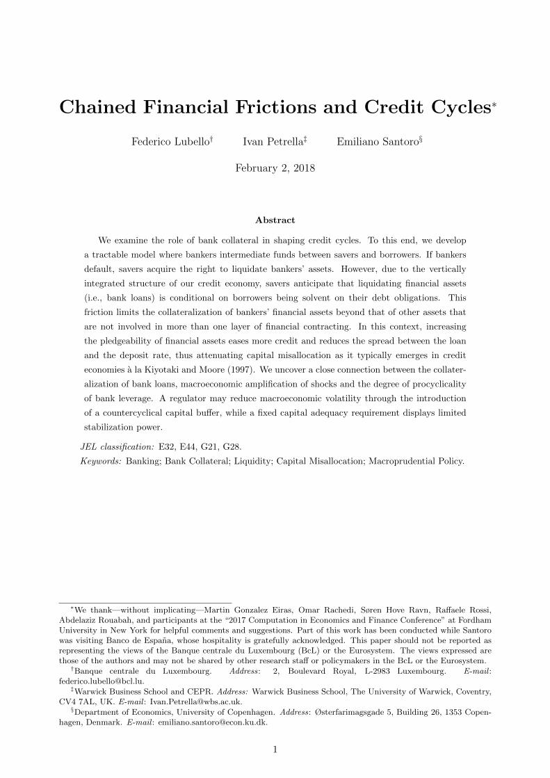
borrowers’ budget and collateral constraint, respectively. The first-order conditions are:

8

∂LBt∂bBt

= 0⇒ −βBRBEtϑBt+1 + ϑBt − υt = 0; (8)

∂LBt∂kBt

= 0⇒ −ϑBt qt + βBEt[ϑBt+1qt+1

]+ βBEt

[ϑBt+1αt+1

]+ ωυtEt

[qt+1

RB

]= 0. (9)

Condition (8) implies that a marginal decrease in borrowing today expands next period’s utility and

relaxes the current period’s borrowing constraint. As for (9), acquiring an additional unit of capital

today allows to expand future consumption not only through the conventional capital gain and

dividend channels, but also through the feedback effect of the expected collateral value on the price

of capital. As we consider linear preferences (i.e., ϑBt = ϑB = 1), (8) implies υt = υ = 1− βBRB.7

Thus, the collateral constraint binds in the neighborhood of the steady state as long as RB < 1/βB,

which is imposed throughout the rest of the analysis. Finally, (9) can be rewritten as

qt =βBRB + ω

(1− βBRB

)RB

Etqt+1 + βBEtαt+1. (10)

2.3 Bankers

Bankers’ primary activity consists of intermediating funds between savers and borrowers. However,

their ability to attract savers’ financial resources is bounded by the limited enforceability of the

deposit contracts, given that bankers may divert assets for personal use (see also Gertler and Kiy-

otaki, 2015). At this stage of the analysis we abstract from the implementation of regulatory bank

capital ratios to discourage bankers’ moral hazard behavior, while focusing on the characteristics of

the deposit contract. We assume that, upon bankers’ default, savers acquire the right to liquidate

bankers’ asset holdings.8 At the time of contracting the amount of deposits, though, the liquida-

tion value of bankers’ assets is uncertain. In this respect, the enforcement problem is isomorphic

to that characterizing bankers’ lending relationship with the borrowers. However, due to the verti-

cally integrated structure of the credit economy, we envisage an additional friction that limits the

pledgeability of bank loans beyond that of capital. While real assets remain in the availability of the

bankers for the entire duration of the deposit contract—so that savers can frictionlessly liquidate

them in case of bankers’ default—the resources corresponding to bankers’ financial claims are in

the availability of the borrowers. Therefore, from the perspective of the savers the possibility to

liquidate bBt in the event of a default of the banking sector goes beyond the capacity of the bankers

to honor the deposit contract, while being subordinated to borrowers’ solvency. In light of this, we

assume that savers account for a transaction cost they would have to bear for seizing bank loans:

(1− ξ) bBt , where ξ ∈ [0, 1] indexes savers’ perceived liquidity of bankers’ financial assets. In the

extreme case savers regard bank loans as completely illiquid and do not accept them as collateral, ξ

is set to zero (i.e., financial frictions are no longer chained), while ξ = 1 corresponds to a situation

in which savers attach no risk to their ability of liquidating financial assets in case bankers’ default.

7Steady-state variables are reported without the time subscript.8There are two main considerations why this assumption is a reasonable one: first, savers have no direct use of

the collateral assets; second, even if collateral assets represent an attractive investment opportunity, savers have noexperience in hedging.

9

To derive the renegotiation outcome, we assume that with probability 1 − χ savers expect

to recover no collateral, while with probability χ the expected recovery value is Etqt+1kIt + ξbBt ,

where kIt denotes bankers’ holdings of capital and ξbBt represents the amount of bank loans held as

collateral, net of transaction costs. This implies the following default scenarios:

1. Savers expect to recover Etqt+1kIt + ξbBt . Since savers expect to expropriate the stock of

real and financial assets after bearing a transaction cost (1− ξ) bBt , bankers have to make a

payment that leaves savers indifferent between liquidation and allowing borrowers to preserve

the stock of collateral assets. This requires bankers to make a payment at least equal to

Etqt+1kIt + ξbBt , so that the ex-post value of defaulting for the bankers is:

RSbSt − Etqt+1kIt − ξbBt . (11)

2. Savers expect to recover no collateral. If the liquidation value is zero, liquidation is clearly

not the best option for the savers. Therefore, bankers have no incentive to pay deposits back.

The ex-post default value in this case is:

RSbSt . (12)

Enforcement requires that the expected value of non-defaulting is not smaller than the expected

value of defaulting, so that:

0 ≥ χ[RSbSt − Etqt+1k

It − ξbBt

]+ (1− χ)RSbSt , (13)

which reduces to

RSbSt ≤ χ(Etqt+1k

It + ξbBt

), (14)

according to which deposits should be limited from above by a fraction of the discounted expected

collateral value. Notably, bankers’ collateral constraint embodies the notion that real and financial

assets have different degrees of liquidity (see also Bernanke and Gertler, 1985).9 In fact, (14) is

reminiscent of the liquidity constraint envisaged by Benigno and Nistico (2017), where safe and

pseudo-safe assets co-exist and both contribute to set the maximum amount of resources available

for consumption. In their case, while the entire stock of safe assets (i.e., money) is available

to finance private expenditure, only a fraction of pseudo-safe assets can be employed to cover

consumption, hence displaying less than perfect liquidity.

Some considerations are in order about the role of the capital goods held by the bankers. First,

this asset mainly serves as a buffer against which the intermediary is trusted to be able to meet

its financial obligations.10 In addition, kIt is important in that it breaks the tight link between

9As χ affects the collateralization of both real and financial assets, in the remainder we will refer to ‘financialcollateralization’ as the degree of pledgeability of bank loans that is exclusively captured by their liquidity, as indexedby ξ.

10Broadly speaking, kIt may be seen as corresponding to bankers’ security holdings, which are typically more liquid,as compared with bank loans.

10

deposits and lending—which would be otherwise embodied by a binding deposit contract—thus

allowing for the possibility that a countercyclical ‘flight to quality’ drives the supply of credit. In

the present context, such an effect would translate into bankers’ allocating relatively more resources

to capital investment—which, unlike bank loans, does not bear any risk of default—during adverse

periods. In turn, this mechanism may open the route to the emergence of credit crunch episodes

(Bernanke and Lown, 1991). Finally, as in Bernanke and Gertler (1985) we assume that capital

is productive, being employed by bankers to invest in projects on their own behalf.11 Specifically,

bankers’ production technology is assumed to feature the following properties:

yIt = αtG(kIt−1), (15)

with G′> 0, G

′′< 0, G

′(0) > % > G

′(1),12 and

% ≡RBβB

[RS(1− βI

)− χ

(1− βIRS

)]RSβI [RB (1− βB)− ω (1− βBRB)]

, (16)

where βI denotes bankers’ discount factor and (16) is required to ensure an internal solution in

which both bankers and borrowers demand capital.13

Bankers’ flow-of-funds constraint reads as:

cIt + bBt +RSbSt−1 + qt(kIt − kIt−1) = bSt +RBbBt−1 + yIt , (17)

where cIt denotes bankers’ consumption. The Lagrangian for bankers’ optimization reads as

LIt = E0

∞∑t=0

(βI)t {

cIt − ϑIt [cIt +RSbSt−1 + bBt + qt(kIt − kIt−1) (18)

−bSt −RBbBt−1 − αtG(kIt−1)]− δt(bSt − χ

qt+1

RSkIt − χξ

bBtRS

)},

where ϑIt and δt are the multipliers associated with bankers’ budget constraint and enforcement

constraint, respectively. The first-order conditions are:

11One can conceive the banking sector as a two-member household sharing externalities and pooling resources. Onemember of the household specializes in credit intermediation, whereas the other specializes in production. Therefore,the first household member has to determine the amount of resources to be lent to the borrower, as well as the amountto be extended to the other member of the household. When funds are kept within the household, agency costs aremitigated. Yet, this comes at the cost of bankers-producers accessing a decreasing returns to scale technology.

12Assuming a decreasing returns to scale technology available to the borrowers would not alter our key results. Aswe will see in the next section, it is the relatively higher impatience of the borrowers, combined with their collateralconstraint, that endows them with a suboptimal stock of capital. This point is also discussed in KM. Introducing adecreasing returns to scale technology would only hinder the analytical tractability of the model.

13The role of this property will be discussed further in Section 4.1.

11

∂LIt∂bSt

= 0⇒ −RSβIEtϑIt+1 + ϑIt − δt = 0; (19)

∂LIt∂bBt

= 0⇒ RBβIEtϑIt+1 − ϑIt +

1

RSχξδt = 0; (20)

∂LIt∂kIt

= 0⇒ −ϑIt qt + βIEt[ϑIt+1qt+1

]+ βIEt

[ϑIt+1αt+1G

′(kIt )

]+ δtχ

Et [qt+1]

RS= 0. (21)

As we assume linear preferences, ϑIt = ϑI = 1. Therefore, conditions (19) and (20) imply that

the financial constraint holds with equality in the neighborhood of the steady state (i.e., δt = δ > 0)

as long as (i) RSβI < 1 and (ii) RBβI < 1. Specifically, condition (i) implies that bankers are

relatively more impatient than savers,14 while condition (ii) implies that, unless either χ or ξ equal

zero, bankers charge a lending rate that is lower than their rate of time preference, as extending

loans allows them to relax their financial constraint:

RB =RS − χξ

(1− βIRS

)βIRS

, (22)

from which it is possible to write down the spread between the loan and the deposit rate:

RB −RS =βS − βI

βIβS− χξ 1− βIRS

βIRS. (23)

The first term on the right-hand side of the equality is the spread that would prevail if bankers

could not borrow off their loans (i.e., if χξ = 0), while the second term captures how bankers’

financial constraint affects their ability to intermediate funds. Increasing χ and/or ξ compresses

the spread. As implied by (20), greater pledgeability of financial assets increases the collateral

value that savers expect to recover in case of bankers’ default. This relaxes the financial constraint,

eases more deposits and translates into a higher credit supply, thus compressing the lending rate.

Although (20) and (21) imply that an increase in either real or financial assets relaxes borrowers’

financial constraint, the distinction between the two types of collateral has crucial implications for

bankers’ incentives to intermediate funds between savers and borrowers. On one hand, while

increasing kIt expands bankers’ lending capacity, it also exerts a negative externality on borrowers’

demand for credit by decreasing their collateral. On the other hand, increasing bBt attenuates the

debt-enforcement problem between bankers and borrowers, as implied by the reduction of the spread

between the loan and the deposit rate. As it will be discussed in Section 4.2, such a distinction has

key implications for equilibrium dynamics.

Finally, from (21) we can retrieve the Euler equation governing bankers’ investment in real

assets:

qt =RSβI + χ

(1− βIRS

)RS

Etqt+1 + βIEt

[αt+1G

′(kIt )

]. (24)

Note that by relaxing (i) and allowing for βIRS = 1 (i.e., assuming that bankers are as impatient

as savers), (24) reduces to lenders’ Euler equation in the conventional direct-credit economy a la

KM. Under these circumstances, bankers are no longer financially constrained. As we shall see in

14In this respect, imposing βIRS = 1 reduces the model to the conventional KM economy.

12

the next section, this implies both a higher loan rate and a higher user cost of capital from the

perspective of the bankers/lenders, as compared with what observed when bankers face a binding

collateral constraint. These properties will play a crucial role for both the long-run and the short-

run behavior of the model economy.

2.4 Market Clearing

To close the model, we need to state the market-clearing conditions. We know that the total supply

of capital equals one: kIt + kBt = 1. As for the consumption goods market, the aggregate resource

constraint reads as:

yt = yIt + yBt , (25)

where yt denotes the total demand of consumption goods.

The aggregate demand and supply for credit are given by the two enforcement constraints

(holding with equality) faced by borrowers and bankers, respectively:

bBt = ωEtqt+1k

Bt

RB, (26)

bBt =1

ξχ

(RSbSt − χEtqt+1k

It

). (27)

Finally, as savers are indifferent between any path of consumption and savings, the amount of

deposits depends on bankers’ capitalization. Thus, the markets for deposits and final goods are

cleared according to the Walras’ Law.

3 Steady State

Financial frictions characterizing both the savers-bankers relationship and the bankers-borrowers

relationship deeply affect the welfare properties of the model. Examining their interaction in the

long-run is key for understanding the propagation of technology shocks.

In the remainder we impose, without loss of generality, G(kIt−1) =(kIt−1

)µ, with µ ∈ [0, 1].

Evaluating (10) in the non-stochastic steady state returns:

q =RBβB

(1− βB)RB − ω (1− βBRB). (28)

From (24) we retrieve the marginal product of bankers’ capital, as a function of its price:

G′(kI) =

RS(1− βI

)− χ

(1− βIRS

)RSβI

q, (29)

so that Equations (28), (29) and kI +kB = 1 pin down borrowers’ and bankers’ holdings of capital.

In turn, these allow us to characterize the key inefficiency at work in the economy. Importantly,

financial collateralization only affects the steady state of the economy through its impact on RB,

which in turn influences the capital price through borrowers’ Euler, as implied by (28).15

15In light of this, envisaging savers that invest in real assets in place of the bankers would alter neither the role of

13

Figure 1: Steady-state equilibrium

Figure 1 provides a sketch of the long-run equilibrium of the economy. On the horizontal axis,

borrowers’ demand for capital is measured from the left, while bankers’ demand from the right. The

sum of the two equals one. On the vertical axis we report the marginal product of capital of both

borrowers and bankers. Borrowers’ marginal product of capital is indicated by the line ACE∗, while

bankers’ marginal product is represented by the line DE0E∗. The first-best allocation would be

attained at E0, where the product of capital owned by the bankers and the borrowers is the same,

at the margin. In our economy, however, the steady-state equilibrium is at E∗, where the marginal

product of capital of the borrowers (mpkB = 1) exceeds that of the bankers (mpkI = %). That is,

relative to the first best too little capital is used by the borrowers, due to their financial constraint.

As discussed by KM, this type of capital misallocation implies a loss of output relative to the

first-best, as indicated by the area CE0E∗.16 The following remark elaborates on the relationship

between borrowers’ and bankers’ marginal product of capital:

Remark 1 As long as βB < βI , bankers’ marginal product of capital is lower than that of the

borrowers.

In fact, imposing G′(kI) < 1 returns the following inequality:

βB − βI <βBχ

(1− βIRS

) (RB + ωξ

)RS (RB − ω)

. (30)

liquidity of bankers’ financial collateral, nor the key aggregate implications of the model.16The area under the solid line, ACE∗D, is the steady-state output.

14

As we assume βB < βI , the left-hand side of the inequality is negative, while its right-hand side

is positive, given that both βIRS < 1 and RB > ω hold by assumption. Therefore, a distinctive

feature of the equilibrium is that the marginal product of borrowers’ capital is higher than that

of the bankers, given that the former cannot borrow as much as they want. As a result, any shift

in capital usage from the borrowers to the bankers will lead to a first-order decline in aggregate

output, as it will become evident when exploring the linearized economy.

So far the present economy is isomorphic to that put forward by KM, as the suboptimality of the

steady-state equilibrium allocation ultimately rests on borrowers’ financial constraint. However,

it is important to note that combining limited enforceability of both deposit and loan contracts

induces bankers to hold less capital and increase their marginal product—thus setting the steady-

state equilibrium on a more efficient allocation—as compared with the baseline KM economy. To

see this, it sufficies to set βIRS = 1, so as to reduce the model to a direct-credit economy where

savers and bankers have identical degrees of impatience. Notably, in this case the productivity

gap between bankers and borrowers is higher than that obtained in the economy with financial

intermediation. This is due to the lenders charging a higher loan rate and attaining a higher

steady-state user cost of capital, which exacerbates the inefficiency in capital allocation. In Figure

1 this additional loss of output, relative to the first-best allocation, is captured by the trapezoid

CKMCE∗E∗KM (where E∗KM indicates the steady-state equilibrium in the KM setting).

In light of this key property, the next step in the analysis consists of understanding how the

collateralization of different types of bank assets impacts on capital misallocation. To this end, we

define the productivity gap between borrowers and bankers as

mpkB −mpkI ≡ ∆ = 1− %. (31)

As far as the effect of χ on the productivity gap is concerned, this is not unambiguous: on one

hand, raising χ inflates the steady-state capital price by compressing the intermediation spread, as

embodied by (22); on the other hand, a higher χ increases bankers’ marginal benefit of relaxing the

collateral constraint by investing into an extra unit of capital, as embodied by (21): as a result,

bankers’ have a higher incentive to accumulate capital, so that the first factor on the right-hand

side of (29) decreases in χ. As it will be detailed in the next section, these competing forces tend to

offset each other, so that bankers’ deposit-to-value ratio has little influence on capital misallocation

and the propagation of technology disturbances.

As for the pledgeability of bank loans, the following summarizes the impact of financial collat-

eralization on the productivity gap:

Proposition 1 Increasing the pledgeability of bank loans (ξ) reduces the gap between bankers’ and

borrowers’ marginal product of capital (∆).

Proof. See Appendix A.

Notably, a higher degree of financial collateralization expands bankers’ lending capacity and

compresses the spread charged over the deposit rate. In turn, lower lending rates allow borrow-

ers to increase their borrowing capacity through a higher collateral value, ceteris paribus. The

15

combination of these effects is such that mpkI unambiguously increases in the degree of financial

collateralization, reducing the productivity gap with respect to the borrowers. This factor will play

a key role in determining the size of the response of gross output to a technology shock, as it will

be detailed in Section 4.1.

4 Equilibrium Dynamics

To examine equilibrium dynamics we preliminarily log-linearize the key behavioral rules and con-

straints around the non-stochastic steady state, where the incentive compatibility constraints (5)

and (14) are assumed to hold with equality.17 This local approximation method is accurate to the

extent that we limit the technology shock to be bounded in the neighborhood of the steady state,

so that neither borrowers’ nor bankers’ default occurs as an equilibrium outcome. As for borrowers’

Euler equation (10):

qt = φEtqt+1 + (1− φ)Etαt+1, (32)

where φ ≡ βBRB+ω(1−βBRB)RB

. As for the bankers’ Euler equation (24):

qt = λEtqt+1 + (1− λ)Etαt+1 +1− λη

kBt , (33)

where λ ≡ RSβI+χ(1−βIRS)RS

and η−1 is the elasticity of the bankers’ marginal product of capital

times the ratio of borrowers’ to bankers’ capital holdings in the steady state (i.e., η ≡ 1−kBkB(1−µ)

).

Once we obtain the solutions for qt and kBt as linear functions of the technology shifter, we can

determine closed-form expressions for the equilibrium path of other variables in the model. We

first focus on (32), whose forward-iteration leads to:

qt = γαt, (34)

where γ ≡ 1−φ1−φρρ > 0. With this expression for qt, we can resort to (33), obtaining

kBt = vαt, (35)

where v ≡ η1−λ

(λ−φ)(1−ρ)ρ1−φρ > 0. Thus, it is possible to linearize total production in the neighborhood

of the steady state, obtaining:

yt = αt + ∆yB

ykBt−1, (36)

According to (36), the dynamics of gross output is shaped by αt, as well as by borrowers’ capital

holdings at time t−1: the second effect captures the endogenous propagation of productivity shifts

on gross output. In fact, yt depends on the past history of shocks not only through the first-round

impact of αt, but also through the effect of αt−1 on kBt−1, as implied by (35). In light of this, we

can rewrite (36) as

yt = $αt−1 + ut (37)

17Variables in log-deviation from their steady-state level are denoted by a ”ˆ”.

16

where$ ≡ ρ+v∆yB

y . According to (37), eliminating the key source of steady-state inefficiency—i.e.,

attaining ∆ = 0—implies that total output’s departures from the steady state would track the path

of the technology shock, so that the model would feature no endogenous propagation of produc-

tivity shifts.18 Moreover, we need to recall that envisaging limited enforceability of both deposit

and loan contracts reduces capital misallocation as it emerges in the original KM economy, thus

compressing ∆ with respect to the case in which RSβI = 1. In this respect, the model produces a

‘banking attenuator’ that entirely rests on the functioning of financial frictions in banking activity,

as compared with analogous effects stemming from the procyclicality of the external finance pre-

mium (Goodfriend and McCallum, 2007) or monopolistic competition in the intermediation activity

and staggered interest rate-setting schemes (Gerali et al., 2010).

4.1 Financial Collateral and Macroeconomic Amplification

We have now lined up the elements necessary to examine how savers’ perceived liquidity of bankers’

financial assets affects the amplitude of credit cycles. In this respect, there are three different

channels through which ξ affects the endogenous response of total production to a technology

shock:∂$

∂ξ= ∆

yB

y

∂v

∂ξ+ v

yB

y

∂∆

∂ξ+ v∆

∂(yB/y

)∂ξ

. (38)

As for the first term on the right hand side of (38), Proposition 2 details the effect induced by

a marginal change in the degree of financial collateralization on the response of borrowers’ capital

holdings to the technology shock.

Proposition 2 Increasing the degree of collateralization of bank loans (ξ) attenuates the impact of

the technology shock on both borrowers’ holdings of capital and the capital price.

Proof. See Appendix A.

According to Proposition 2 the sensitivity of borrowers’ capital holdings to the technology

shifter decreases in ξ. The intuition for this is twofold: first, increasing ξ determines a more even

distribution of capital goods, as reflected by the drop in η; second, being able to pledge a higher

share of financial assets reinforces the sensitivity of the capital price to the capital gain component

in borrowers’ Euler equation, φ, through the drop in the loan rate, while reducing the sensitivity

to the dividend component (i.e., the shock). These effects are mutually reinforcing and ultimately

exert a negative force on the overall degree of macroeconomic amplification of the system.

Turning our attention on the other two terms on the right hand side of (38), we know from

Proposition 1 that the productivity gap between borrowers and bankers shrinks as financial col-

lateralization increases (i.e., ∂∆/∂ξ < 0). Finally, it is immediate to prove that the last term on

the right-hand side of (38) is positive, in light of greater collateralization of bank loans inducing

a reallocation of capital from the bankers to the borrowers. In turn, this transfer implies both

18This property echoes the role of the steady-state inefficiency for short-run dynamics in the KM model. In theirsetting, closing the gap between lenders’ and borrowers’ marginal product of capital would imply no response at allto a productivity shift. In this respect, the key difference between the two frameworks lies in that we assume anautoregressive shock, while they consider an unexpected one-off shift in technology.

17

Figure 2: Business cycle amplification

µ

ξ

0 0.2 0.4 0.6 0.8 1

0

0.2

0.4

0.6

0.8

1

1

1.1

1.2

1.3

1.4

1.5

1.6

Figure 2 graphs $ as a function of ξ and µ, under the following parameterization: βS = 0.99, βI = 0.98, βB = 0.97,ρ = 0.95, χ = ω = 1. The white area denotes inadmissible equilibria where bankers’ capital holdings are virtuallynegative.

a first-order positive effect on yB and a (milder) second-order positive impact on y, so that the

overall effect on yB/y is positive.19

To sum up, an increase in ξ causes competing effects on $. First, greater financial collater-

alization depresses the pass-through of αt−1 on borrowers’ capital holdings, which in turn affect

total production with a lag. Second, raising ξ exerts two distinct effects on the pass-through of

kBt−1 on yt: on one hand, bankers’ marginal product of capital increases, implying a reduction of

the productivity gap; on the other hand, borrowers’ contribution to total production increases,

as the reduction in the productivity gap reflects higher capital accumulation in the hands of the

borrowers. The sum of these three forces potentially leads to mixed results on output amplifica-

tion, as captured by the second-round effect of technology disturbances. To address this, we plot

$ as a function of ξ and µ.20 The aim of this exercise is to examine the direction of the overall

effect exerted by financial collateralization on macroeconomic volatility, rather than quantifying an

empirically plausible multiplier emerging from the interaction of bankers’ and borrowers’ financial

19Recall that total output is an increasing function of borrowers’ capital. Therefore, the drop in yI following amarginal increase in ξ is lower than the corresponding rise in yB .

20The discount factors are set in accordance with our assumptions about the relative degree of impatience of thethree agents in the economy and are broadly in line with existing (quarterly) calibrations involving economies withheterogeneous agents: βS = 0.99, βI = 0.98, βB = 0.97. We set ρ = 0.95, in line with the empirical evidence showingthat technology shocks are generally small, but highly persistent (see, e.g., Cooley and Prescott, 1995). As for χand ω , they are both set to 1, so as to ensure a wider set of admissible combinations of ξ and µ that correspondto positive holdings of capital for both bankers and borrowers. This is clearly displayed by the robustness evidencereported in Appendix C, which shows that different combinations of χ and ω are close to irrelevant regarding theeffect of financial collateralization on macroeconomic amplification. Moreover, Figure C1 shows that varying χ hasvirtually no effect on the amplitude of the response to the technology shock, in light of the competing effects exertedon bankers’ marginal product of capital.

18

constraints.21 As it emerges from Figure 2, increasing ξ compresses $, at any level of µ. By

contrast, increasing the income share of capital in bankers’ production technology amplifies the

second-round response of output. This is because µ amplifies the productivity gap through its

positive effect on η.22 All in all, the general picture emerging from this exercise is that allowing

for greater financial collateralization attenuates the overall degree of amplification of technology

disturbances. The next subsection examines how this property reflects into cyclical movements

in bank leverage, whose behavior is key to understanding how bankers’ balance sheet affects the

amplitude of credit cycles.

4.2 The Role of Leverage

To enlarge our perspective on the amplification/attenuation induced by bankers’ financial collateral,

we take a closer look at their balance sheet. To this end, we define bankers’ equity as the difference

between the value of total assets (i.e., loans and capital) and liabilities (i.e., deposits):

eIt = bBt + qtkIt − bSt , (39)

with leverage defined as the ratio between loans and equity: levIt = bBt /eIt .

Figure 3 reports the response of selected variables to a one-standard deviation shock to tech-

nology.23 As implied by (36), on impact output responds one-to-one with respect to the shock,

regardless of the degree of financial collateralization. However, as ξ increases the second-round re-

sponse is gradually muted. To complement our analytical insight and provide further intuition on

this channel, we examine the behavior of a set of variables involved in bankers’ intermediation activ-

ity. In this respect, note that deposits tend to decline at low values of ξ, while increasing as bankers

can pledge a higher share of their financial assets. The reason for this can be better understood

by recalling the nature of the interaction between bankers’ financial and real assets. The interplay

takes place on two levels: on one hand, both assets have a positive effect on savers’ deposits, as

embodied by (14); on the other hand, it is possible to uncover a crowding out effect, as increasing

bankers’ real asset holdings exerts a negative force on lending by reducing borrowers’ collateral.

How do these properties affect the transmission of an expansionary technology shock? Due to the

capital productivity gap between borrowers and bankers, the technology shift necessarily causes a

decline of bankers’ real assets, thus expanding borrowers’ capital and borrowing.24 Therefore, in

21We leave this task for future research employing a large-scale dynamic general equilibrium model.22It is important to emphasize that increasing µ may violate the condition G

′(0) > % > G

′(1), which ensures an

interior solution as for how much capital bankers should hold in the neighborhood of the steady state. To see why

this is the case, recall that µ(kI

)µ−1= %. Increasing µ inflates bankers’ marginal product of capital, while leaving

their user cost unaffected. Thus, as µ increases bankers are induced to hold an increasing stock of capital, so thatthe equality holds. An important aspect is that this effect tends to kick in earlier as ξ declines. This is becausea drop in the degree of financial collateralization depresses bankers’ user cost of capital. Therefore, as ξ declinesand µ increases the set of steady-state allocations in which both bankers and borrowers hold capital restricts, as thecondition % > G

′(1) is eventually violated and borrowers’ may virtually end up with negative capital holdings.

23The baseline parameterization is the same as that employed in Figure 2. As for µ, we impose a rather conservativevalue, 0.4, which allows us to obtain a finite distribution of capital in the steady state.

24This is a distinctive feature of lender-borrower relationships involving the collateralization of a productive asset.In fact, it is possible to show that, following a positive technology shock, the major reallocation of land from thelenders to the borrowers is only attenuated by relaxing the hypothesis of zero aggregate investment – as in the KMbaseline framework – while the direction of the transfer is not inverted.

19

equilibrium deposits are influenced by two opposite forces, namely an expansion in the amount of

bankers’ financial assets and a contraction in their stock of real assets. In this respect, the implied

allocation of bankers’ assets reflects a countercyclical flight to quality pattern (see, inter alia, Lang

and Nakamura, 1995): during expansions (contractions), bankers increase (decrease) their holdings

of the inherently riskier assets—bank loans—while decreasing (increasing) their capital holdings,

which do not bear any risk of default.

Figure 3: Impulse responses to a positive technology shock

Notes. Responses of selected variables to a one standard-deviation shock to technology, under the following parame-terization: βS = 0.99, βI = 0.98, βB = 0.97, ρ = 0.95, χ = ω = 1, µ = 0.4.

How do these diverging forces translate in terms of bankers’ ability to attract deposits and

leverage? As ξ drops the impact of bank loans is gradually muted and deposits eventually track

the dynamics of bankers’ capital. In this context, the contraction of bankers’ real asset overcomes

the drop in deposits, so that lending expands in excess of bank equity, potentially leading to an

increase in leverage. In fact, a procyclical leverage ratio is associated with a relevant degree of

macroeconomic amplification, when bankers’ financial assets are regarded as relatively illiquid.

Figure 3 shows this tends to be the case for ξ < 0.5, under our baseline parameterization.

5 Welfare and Capital Adequacy Requirements

The positive analysis so far has shown that limited enforceability of deposit contracts may reduce

the productivity gap between borrowers and lenders, which is key to quantify the amplitude of credit

cycles. In light of this, our next objective is to understand to which extent a regulator may promote

a more efficient allocation of productive capital by ‘leaning against’ capital misallocation. In this

respect, the Chancellor of the Exchequer has explicitly indicated that—conditional on enhancing

the resilience of the financial system—the Financial Policy Committee at the Bank of England

20

should intend the pursual of productive capital allocation efficiency as part of its macroprudential-

policy mandate:

”Subject to achievement of its primary objective, the Financial Policy Committee

(FPC) should support the Government’s economic objectives by acting in a way that,

where possible, facilitates the supply of finance for productive investment provided by

the UK’s financial system.” (Remit and Recommendations for the Financial Policy

Committee, HM Treasury, July 8, 2015).

In fact, our economy lends itself to the analysis of this particular problem, in light of the strict

connection between the capital productivity gap between borrowers and bankers and the amplitude

of credit cycles.25 To this end, we introduce two complementary tools of regulation. First, we

assume deposit insurance, which ensures that savers do not suffer a loss in the event of bankers’

default.26 A direct implication of such a measure is to shift the risk of bankers’ default to the

government (or a hypothetical interbank deposit protection fund), so that the renegotiation of

deposit contracts is redundant and bankers’ financial constraint may be discarded. However, in

order to mitigate bankers’ moral hazard behavior, the regulator imposes an explicit capital adequacy

requirement (see, e.g., Van den Heuvel, 2008). According to this regulatory constraint, equity needs

to be at least a fraction θ of the loans, for bankers to be able to operate:

eIt ≥ θbBt , θ ∈ [0, 1] , (40)

where θ denotes the capital-to-asset ratio.

Appendix B reports bankers’ optimization problem under (40). In this case, the equilibrium

loan rate reads as

RB =RS − (1− θ)

(1− βIRS

)βI

. (41)

Notably, (41) is isomorphic to (22), with RB increasing in the capital-to-asset ratio. To provide an

intuition for this, we combine (40) with (39), obtaining:

bSt ≤ qtkIt + (1− θ) bBt . (42)

As embodied by (42), imposing a capital-to-asset ratio to bankers’ intermediation activity amounts

to constrain deposits from above by the current value of bankers’ collateral, with the implied degree

of pledgeability of bank loans being a negative function of θ. In fact, there is a direct mapping

between the capital-to-asset ratio implicit in the capital requirement constraint imposed by the

regulator and the degree of collateralization of bank loans as it emerges from the incentive compat-

ibility constraint (14), which is derived in the absence of any form of deposit insurance. Intuitively,

a higher leverage (lower capital) ratio implies a riskier exposure of the financial intermediary. This

25Notably, our model abstracts from trade-offs that impose the policy-maker to balance the incentive to improvethe allocation of productive capital with an alternative financial stability objective, as in Gertler and Kiyotaki (2015),inter alia. However, our primary interest is to understand how far the policy-maker can go so as to resolve the keydistortion in the credit economy, so that there is no need to introduce additional propagation mechanisms that wouldonly hinder the analytical tractability of the model.

26As in Van den Heuvel (2008), deposit insurance is left unmodeled, though it is argued that it generally improvesbanks’ ability to extend credit (see Diamond and Dybvig, 1983).

21

Figure 4: Impulse response under θ = 0 and θ = θ∆=0

Notes. Responses of selected variables to a one standard-deviation shock to technology, under the following parame-terization: βS = 0.99, βI = 0.98, βB = 0.97, ρ = 0.95, χ = ω = 1, µ = 0.4.

translates into greater transaction costs savers would have to bear in order to seize bank loans in

the event of bankers’ default. In turn, these costs have a direct impact on degree of collateralization

of bankers’ financial assets that is implicit in (40).

Therefore, it should come as no surprise that, absent any trade-off between enhancing capital

allocation and ensuring financial stability, the optimal policy consists of setting the capital-to-asset

ratio to its lower bound. Along with minimizing the fraction of bank assets that can be financed by

issuing deposit liabilities, θ = 0 contracts the intermediation spread, thus ensuring a more efficient

allocation of capital between bankers and borrowers. Figure 4—which reports the response of the

economy to a positive technology shock under this policy—confirms this view. Nevertheless, it

is important to notice that even a null capital ratio is not enough to neutralize the endogenous

propagation channel stemming from capital misallocation, as stated by the next proposition.

Proposition 3 The gap between bankers’ and borrowers’ marginal product of capital (∆) cannot

be closed by setting the capital-to-asset ratio (θ) within the range of admissible values.

Proof. See Appendix A.

To dig deeper on this property, Figure 5 maps the spread between the loan and the deposit

rate (y-axis) and the productivity gap (x-axis), for different values of the capital-to-asset ratio (θ)

and the loan-to-asset ratio applying to the borrowers (ω). As we move down along each locus,

θ decreases from its upper bound to the value consistent with ∆ = 0. The color of a given line

switches from green to blue when θ drops below its lower bound. In line with Proposition 3, closing

the productivity gap through a capital requirement within the set of its admissible values proves

to be infeasible for the policy maker. However, it is important to acknowledge that higher loan-to-

22

Figure 5: Interaction between the capital-to-asset and the loan-to-value ratios

Notes. Figure 5 maps RB − RS (y-axis) and ∆ (x-axis) for different values of θ and ω. As we move down alongeach line, θ decreases from its upper bound to the value consistent with ∆ = 0. The color of a given locus switchesfrom green to blue when θ drops below zero. The rest of the parameters are set as follows: βS = 0.99, βI = 0.98,βB = 0.97, ρ = 0.95, µ = 0.4.

value ratios applying to the loan contracts compress the productivity gap at any value of θ. In fact,

raising ω relaxes borrowers’ collateral constraint, allowing them to increase their capital holdings,

so that bankers’ marginal product of capital increases in equilibrium.

Figure 5 also shows that ∆ = 0 may only be attained at negative values of θ and RB −RS . In

Figure 4—where the capital-to-asset ratio compatible with a null productivity gap is denoted by

θ∆=0—the endogenous propagation of the shock is actually switched off under a negative capital-

to-asset ratio, so that gross output tracks the dynamics of the productivity shifter and leverage

is completely acyclical. However, according to (40), setting θ = θ∆=0 would induce bankers to

hold negative equity, for any level of credit extended. Although we rule this out as an equilibrium

outcome, it is interesting to briefly examine the underlying incentives of the bankers in such a

scenario: according to (42), through a negative capital-to-asset ratio, the regulator implicitly pushes

for an ‘hyper-collateralization’ of bank loans. In turn, this eventually induces bankers to set a loan

rate below the interest rate on deposits, which amounts to subsidizing borrowers’ capital investment

so as to resolve the distortion.

5.1 A Countercyclical Capital Buffer

The normative analysis so far has shown that imposing a constant capital requirement plays a

limited role in smoothing economic fluctuations. Thus, we turn our attention to an alternative

regulatory measure that aims at reducing gross output fluctuations by affecting the cyclicality of

bankers’ balance sheet, without necessarily tackling the distortion stemming from capital misal-

location. To this end, recent years have witnessed an increasing interest of policymakers towards

leaning against credit imbalances, pursuing macroeconomic stabilization through policy rules that

set a countercyclical capital buffer. De facto, countercyclical capital regulation is a key block of the

23

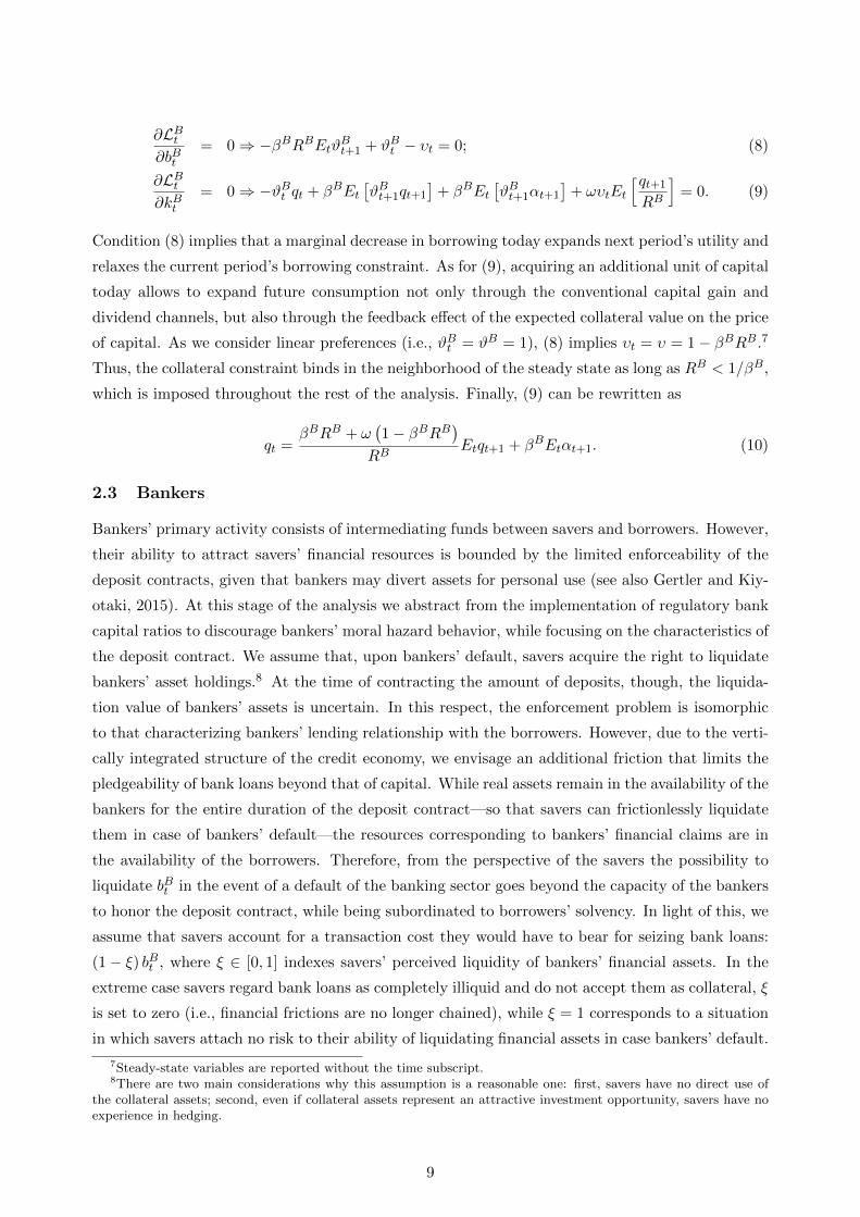
Basel III international regulatory framework for banks.27 Based on the analysis of the transmission

mechanism and the response of bank capital, we now examine the functioning of this type of policy

tool within our framework. Thus, we allow for capital requirements to vary with the macroeconomic

conditions (see, e.g., Angeloni and Faia, 2013, Nelson and Pinter, 2016 and Clerc et al., 2015):

θtθ

=

(bBtbB

)ϕ, ϕ ≥ 0, (43)

where ϕ = 0 implies a constant capital-to-asset ratio, while ϕ > 0 induces a countercyclical capital

buffer.28

By linearizing the time-varying counterpart of (41) in the neighborhood of the steady state we

obtain:

RBt = ψθt, (44)

where ψ = 1−βIRSβIRB

θ is positive, in light of assuming βIRS < 1. We then linearize (43), obtaining:

θt = ϕbBt . (45)

After linearizing borrowers’ financial constraint, we can substitute for bBt in (45) and plug the

resulting expression into (44), so as to obtain:

RBt =ψϕ

1 + ψϕ

(Etqt+1 + kBt

). (46)

Thus, it is possible to establish a connection between the loan rate and borrowers’ expected col-

lateral value. Increasing the responsiveness of the capital-to-asset ratio to changes in aggregate

lending amplifies this channel: raising ϕ implies that marginal deviations of bBt from its steady

state transmit more promptly to the capital-to-asset ratio and, in turn, to the loan rate through

the combined effect of (44) and (45). This induces a feedback effect on borrowers’ capacity to at-

tract external funding, as embodied by their collateral constraint: higher sensitivity of the loan rate

to variations in aggregate lending (i.e., a steeper loan supply function) implies stronger discounting

of borrowers’ expected collateral. In the limit (i.e., as ϕ → ∞) there is a perfect pass-through of

Etqt+1 + kBt on RBt . Therefore, as in the face of a technology shock both terms move in the same

direction and by the same extent, borrowing does not deviate from its steady-state level and output

displays no endogenous propagation.

To assess the stabilization performance of the countercyclical capital buffer rule, in Figure 6 we

set the steady-state capital-to-asset ratio to 8%—in line with the full weight level of Basel I and

the treatment of non-rated corporate loans in Basel II and III—while varying ϕ over the support

[0, 1].29 As expected, at ϕ = 0 (i.e., a capital-to-asset ratio kept at its steady-state level) we observe

27The regulatory framework evolved through three main waves. Basel I has introduced the basic capital adequacyratio as the foundation for banking risk regulation. Basel II has reinforced it and allowed banks to use internalrisk-based measure to weight the share of asset to be hold. Basel III has been brought in response to the 2007-2008crisis, with the key innovation consisting of introducing countercyclical capital requirements, that is, imposing banksto build resilience in good times with higher capital requirements and relax them during bad times.

28According to the Basel III regime, capital regulation can respond to a wide range of macroeconomic indicators.Here we assume it to respond to deviations of bBt from its long-run equilibrium, bB .

29Alternative values of θ would only alter the quantitative implications of the exercise, while not affecting its key

24

Figure 6: Impulse responses under different ϕS

Notes. Responses of selected variables to a one standard-deviation shock to technology, under the following parame-terization: βS = 0.99, βI = 0.98, βB = 0.97, ρ = 0.95, χ = ω = 1, µ = 0.4, θ = 0.08.

the strongest amplification of the output response, while the lending rate and bank leverage are

both acyclical. By contrast, increasing the degree of countercyclicality of the capital buffer proves

to be effective at attenuating the response of gross output to the shock, progressively compressing

bank leverage. Notably, as ϕ → ∞ leverage displays a strong degree of countercyclicality,30 while

lending does not deviate from its steady-state level, as conjectured above. In turn, this results in

the response of gross output featuring no endogenous propagation of technology shocks, despite the

regulator’s policy action is not aimed at tackling capital misallocation and, therefore, the steady-

state productivity gap is not closed.

6 Concluding Remarks

We have devised a credit economy where bankers intermediate funds between savers and borrowers,

assuming that bankers’ ability to collect deposits is affected by limited enforceability: as a result,

if bankers default, savers acquire the right to liquidate bankers’ asset holdings. In this context, we

have examined the role of bank loans as a form of collateral in deposit contracts. Due to the struc-

ture of our credit economy, which may well account for different forms of financial intermediation,

savers anticipate that liquidating financial assets is conditional on borrowers being solvent on their

debt obligations. This friction limits the degree of collateralization of bankers’ financial assets be-

yond that of capital. We have demonstrated three main results: i) limited enforceability of deposit

contracts counteracts the effects of limited enforceability of loan contracts, thus reducing capital

qualitative result.30This is accomplished by setting ϕ = 10, meaning that, for a 1% deviation of debt from its steady-state level, the

capital-to-asset ratio is adjusted from its 8% steady-state level up to 8.8%.

25

misallocation as it emerges in KM; ii) greater collateralization of bankers’ financial assets dampens

macroeconomic fluctuations by reducing the degree of procyclicality of bank leverage; iii) while im-

posing a fixed capital-to-asset ratio to the bankers cannot fully neutralize capital misallocation and

enhance a more efficient allocation of productive capital (thus switching off the associated endoge-

nous propagation channel of productivity shock), a countercyclical capital adequacy requirement

proves to be rather effective at smoothing credit cycles.

Our model is necessarily stylized, though it can be generalized along a number of dimensions.

For instance, a realistic extension could consist of allowing bankers to issue equity (outside equity),

so as to evaluate how a different debt-equity mix may affect macroeconomic amplification over

expansions—when equity can be issued frictionlessly—and contractions, when equity issuance may

be precluded due to tighter information frictions. This factor should counteract the role of financial

assets and help obtaining a countercyclical leverage. In connection with this point, we could also

allow for occasionally binding financial constraints, so as to evaluate how the policy-maker should

behave across contractions, when constraints tighten, and expansions, when constraints may become

non-binding. However, as this type of extensions necessarily hinder the analytical tractability of

our model, we leave them for future research projects based on large-scale models.

26

Appendix A. Proofs

Proof of Proposition 1

As borrowers’ marginal product of capital equals one in the steady state, we restrict our analysis

to the impact of ξ on mpkI :∂mpkI

∂ξ=∂mpkI

∂RB∂RB

∂ξ. (47)

As for the partial derivative of bankers’ marginal product of capital with respect to the loan rate:

∂mpkI

∂RB= − κωβB

κ2RSβI, (48)

where κ ≡ RF(1− βF

)− ω

(1− βFRF

)> 0 and κ ≡ RS

(1− βI

)− χ

(1− βIRS

)> 0, so that

∂mpkI/∂RB < 0.

As for ∂RB/∂ξ < 0, this is negative, in light of assuming βIRS < 1:

∂RB

∂ξ= −

χ(1− βIRS

)βIRS

. (49)

Thus, both factors on the right-hand side of (47) are negative and, since ∂∆/∂ξ = −∂mpkI/∂ξ,increasing ξ inevitably reduces the productivity gap.�

Proof of Proposition 2

We first prove that increasing ξ attenuates the impact of the technology shock on borrowers’

capital-holdings. According to Equation (35) in the main text, v quantifies the pass-through of αt

on kBt . In turn, the marginal impact of ξ on v can be computed as:

∂v

∂ξ=

(λ− φ) (1− ρ) ρ

(1− λ) (1− φρ)

∂η

∂ξ+

(λρ− 1) (1− ρ) ρ

(1− φρ)2

∂φ

∂ξ, (50)

where:∂η

∂ξ=

∂η

∂kB∂kB

∂RB∂RB

∂ξand

∂φ

∂ξ=

∂φ

∂RB∂RB

∂ξ. (51)

Focusing on the second term on the right-hand side of (50), we can show this is negative, as: (i)(λρ−1)(1−ρ)ρ

(1−φρ)2< 0, given that λρ < 1; (ii) ∂φ/∂RB = −ω/

(RB)2< 0; (iii) ∂RB/∂ξ < 0, as implied

by (49).

As for the first term on the right-hand side of (50): (λ−φ)(1−ρ)ρ(1−λ)(1−φρ) > 0. Furthermore:

∂η

∂kB= − 1

(1− µ) (kB)2 < 0

and

∂kB

∂RB=

ω

κRB (µ− 1)

(1

µ

RBβBκRSβIκ

) 1µ−1

< 0, (52)

where κ ≡ RB(1− βB

)− ω

(1− βBRB

)and κ ≡ RS

(1− βI

)− χ

(1− βIRS

). As ∂RB/∂ξ < 0,

also the first term on the right-hand side of (50) is negative. Therefore, ν is a negative function of

ξ.

27

As for the impact of technology shocks on the capital price:

∂γ

∂ξ=∂γ

∂φ

∂φ

∂ξ. (53)

As for ∂γ/∂φ:∂γ

∂φ= − 1− ρ

(1− φρ)2 ρ < 0, (54)

while we already know that ∂φ/∂ξ > 0. Therefore, the overall effect of ξ on γ is negative.�

Proof of Proposition 3

We know that G′(kI) is a decreasing function of θ. Thus, we aim to prove that the gap between

bankers’ and borrowers’ marginal product of capital is greater than zero at θ = 0. To this end, we

combine the capital Euler equations of bankers and borrowers, obtaining:

G′(kI)

∣∣∣θ=0

=RBβB

(RS − 1

)(1− βB)RB − ω (1− βBRB)

.

We then impose G′(kI)

∣∣∣θ=0

< 1 to obtain

RB >ω

1− βB (RS − ω).

As RB∣∣θ=0

=RS(1+βI)−1

βI, all we need to prove is that

RS(1 + βI

)− 1

βI>

ω

1− βB (RS − ω),

which can be manipulated to obtain

(1− βBRS

) [βI(RS − ω

)+RS − 1

]+(RS − 1

)βBω > 0.

As βBRS < 1, it is immediate to verify that both terms on the left-hand side of the last inequality

are positive.�

28

Appendix B. The Model with Capital Requirements

Preliminary, note that combining the capital requirement with the definition of equity returns the

following constraint: bSt ≤ qtkIt + (1− θ) bBt . Thus, the Lagrangian for bankers’ optimization may

be written as:

LIt = E0

∞∑t=0

(βI)t {

cIt − ϑIt [cIt +RSbSt−1 + bBt + qt(kIt − kIt−1) (55)

−bSt −RBbBt−1 − αtG(kIt−1)]− δt[bSt − qtkIt − (1− θ) bBt

]},

where ϑIt = 1 and δt are the multipliers associated with bankers’ budget constraint and the capital

requirement constraint, respectively. The first-order conditions are:

∂LIt∂bSt

= 0⇒ −RSβIEtϑIt+1 + ϑIt − δt = 0; (56)

∂LIt∂bBt

= 0⇒ RBβIEtϑIt+1 − ϑIt + (1− θ) δt = 0; (57)

∂LIt∂kIt

= 0⇒ −ϑIt qt + βIEt[ϑIt+1qt+1

]+ βIEt

[ϑIt+1αt+1G

′(kIt )

]+ δtqt = 0. (58)

In light of these conditions we can derive expressions for both RBt and qt in the presence of a binding

capital requirement constraint:

RB =RS − (1− θ)

(1− βIRS

)βI

, (59)

qt =1

RSEtqt+1 +

1

RSEt

[αt+1I

′(kIt )

]. (60)

29

Appendix C. Robustness Exercises

Figure C.1: Business cycle amplification

! = 0.35, @ = 0.35

0 0.5 1

9

0

0.5

1

! = 0.7, @ = 0.35

0 0.5 1

0

0.5

1

! = 1, @ = 0.35

0 0.5 1

0

0.5

1

! = 0.35, @ = 0.7

0 0.5 1

9

0

0.5

1

! = 0.7, @ = 0.7

0 0.5 1

0

0.5

1

! = 1, @ = 0.7

0 0.5 1

0

0.5

1

! = 0.35, @ = 1

70 0.5 1

9

0

0.5

1

! = 0.7, @ = 1

70 0.5 1

0

0.5

1

! = 1, @ = 1

70 0.5 1

0

0.5

1

Notes. Figure C.1 graphs $ as a function of ξ (y-axis) and µ (x-axis), and for different values of χ and ω,

under the following parameterization: βS= 0.99, βI= 0.98, βB= 0.97, ρ = 0.95. The white area denotes

inadmissible equilibria where bankers’ capital-holdings are virtually negative.

30

References

[1] Angeloni, I. and E. Faia, 2013, Capital Regulation and Monetary Policy with Fragile Banks,

Journal of Monetary Economics, 60:311–324.

[2] Bank of England, 2016, Understanding and Measuring Finance for Productive Investment,

Discussion Paper.

[3] Begenau, J., 2015, Capital Requirements, Risk Choice, and Liquidity Provision in a Business

Cycle Model, mimeo, Harvard Business School.

[4] Benigno, P. and S. Nistico, 2017, Safe Assets, Liquidity and Monetary Policy, American Eco-

nomic Journal: Macroeconomics, 9:182–227.

[5] Bernanke, B.S. and M. Gertler, 1985, Banking in General Equilibrium, NBER Working Papers

1647, National Bureau of Economic Research, Inc.

[6] Bernanke, B. S., M. Gertler and S. Gilchrist, 1999, The Financial Accelerator in a Quantitative

Business Cycle Framework, in Handbook of Macroeconomics, J. B. Taylor and M. Woodford

(eds.), Vol. 1, chapter 21:1341–1393.

[7] Bernanke, B.S. and C. S. Lown, 1991, Credit Crunch, Brookings Papers on Economic Activity,

22:205–248.

[8] Chen, N.-K., 2001, Bank Net Worth, Asset Prices and Economic Activity, Journal of Monetary

Economics, Elsevier, 48:415–436.

[9] Clerc, L., A. Derviz, C. Mendicino, S. Moyen, K. Nikolov, L. Stracca, J. Suarez and A.

P. Vardoulakis, 2015, Capital Regulation in a Macroeconomic Model with Three Layers of

Default, International Journal of Central Banking, 11:9–63.

[10] Cooley, T. F. and E. C. Prescott, 1995, Economic Growth and Business Cycles. Princeton

University Press.

[11] Cordoba, J. C. and M. Ripoll, 2004, Credit Cycles Redux, International Economic Review,

45:1011–1046.

[12] Diamond, D. W. and P. H. Dybvig, 1983, Bank Runs, Deposit Insurance, and Liquidity,

Journal of Political Economy, 91:401–419.

[13] Elenev. V., T. Landovoigt and S. Van Nieuwerburgh, 2017, A Macroeconomic Model with

Financially Constrained Producers and Intermediaries, SSRN Library.

[14] Gerali, A., S. Neri, L. Sessa and F.M. Signoretti, 2010, Credit and Banking in a DSGE Model

of the Euro Area, Journal of Money, Credit and Banking, 42:107–141.

[15] Gersbach, H. and J.-C. Rochet, 2016, Capital Regulation and Credit Fluctuations, forthcom-

ing, Journal of Monetary Economics.

31

[16] Gertler, M. and N. Kiyotaki, 2010, Financial Intermediation and Credit Policy in Business

Cycle Analysis, Handbook of Monetary Economics, in: Benjamin M. Friedman & Michael

Woodford (ed.), 3:547–599.

[17] Gertler, M. and N. Kiyotaki, 2015, Banking, Liquidity, and Bank Runs in an Infinite Horizon

Economy, American Economic Review, 105:2011–2043.

[18] Gertler, M., N. Kiyotaki and A. Queralto, 2012, Financial Crises, Bank Risk Exposure and

Government Financial Policy, Journal of Monetary Economics, 59:17–34.

[19] Goodfriend, M. and B.T. McCallum, 2007, Banking and Interest Rates in Monetary Policy

Analysis: a Quantitative Exploration, Journal of Monetary Economics, 54:1480–1507.

[20] Harris, M., C. C. Opp and M. M. Opp, 2014, Macroprudential Bank Capital Regulation in a

Competitive Financial System, mimeo, University of California, Berkeley (Haas).

[21] Hart, O. and J. Moore, 1994, A Theory of Debt Based on the Inalienability of Human Capital,

Quarterly Journal of Economics 109:841–879.

[22] Hirakata, N., N. Sudo and K. Ueda, 2009, Chained Credit Contracts and Financial Accelera-

tors, forthcoming, Economic Inquiry.

[23] HM Treasury, 2015, Remit and Recommendations for the Financial Policy Committee, 8 July.

Available at http://www.bankofengland.co.uk/financialstability/Documents/fpc/letters

[24] Holmstrom, B. and J. Tirole, 1997, Financial Intermediation, Loanable Funds and the Real

Sector, Quarterly Journal of Economics 112:663–691.

[25] Kiyotaki, N. and J. Moore, 1997, Credit Cycles, Journal of Political Economy, 105:211–248.

[26] Kocherlakota, M. R., 2001, Risky Collateral and Deposit Insurance, The B.E. Journal of

Macroeconomics, 1:1–20.

[27] Krishnamurthy, A., 2003, Collateral Constraints and the Amplification Mechanism, Journal

of Economic Theory, 111:277–292.

[28] Lang, W. and L. Nakamura, 1995, Flight to Quality in Banking and Economic Activity, Journal

of Monetary Economics, 36:145–164.

[29] Martinez-Miera, D. and J. Suarez, 2012, A Macroeconomic Model of Endogenous Systemic

Risk Taking, CEPR Discussion Papers, No. 9134.

[30] Nelson, B. D. and G. Pinter, 2016, Macroprudential Capital Regulation in General Equilibrium,

mimeo, Bank of England.

[31] Van den Heuvel, S. J., 2008, The Welfare Cost of Bank Capital Requirements, Journal of

Monetary Economics, 55:298–320.

32

CHAINED FINANCIAL FRICTIONS AND CREDIT CYCLES

CAHIER D’ÉTUDESWORKING PAPER

N° 115

FEBRUARY 2018

2, boulevard RoyalL-2983 Luxembourg

Tél. : +352 4774-1Fax: +352 4774 4910

www.bcl.lu • info@bcl.lu

FEDERICO LUBELLO IVAN PETRELLA EMILIANO SANTORO