Conjugate Gradient Method

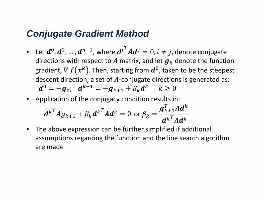
• Let  , , … , , where  0, , denote conjugate directions with respect to  matrix, and let  denote the function gradient,  . Then, starting from  , taken to be the steepest descent direction, a set of  ‐conjugate directions is generated as: 

; 0• Application of the conjugacy condition results in:

0, or

• The above expression can be further simplified if additional assumptions regarding the function and the line search algorithm are made

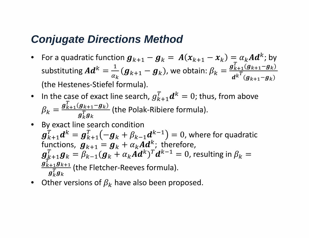
Conjugate Directions Method• For a quadratic function  ; by 

substituting  , we obtain: 

(the Hestenes‐Stiefel formula). • In the case of exact line search,  0; thus, from above 

(the Polak‐Ribiere formula). 

• By exact line search condition 0, where for quadratic 

functions,   ;  therefore, 0, resulting in 

(the Fletcher‐Reeves formula). 

• Other versions of  have also been proposed.

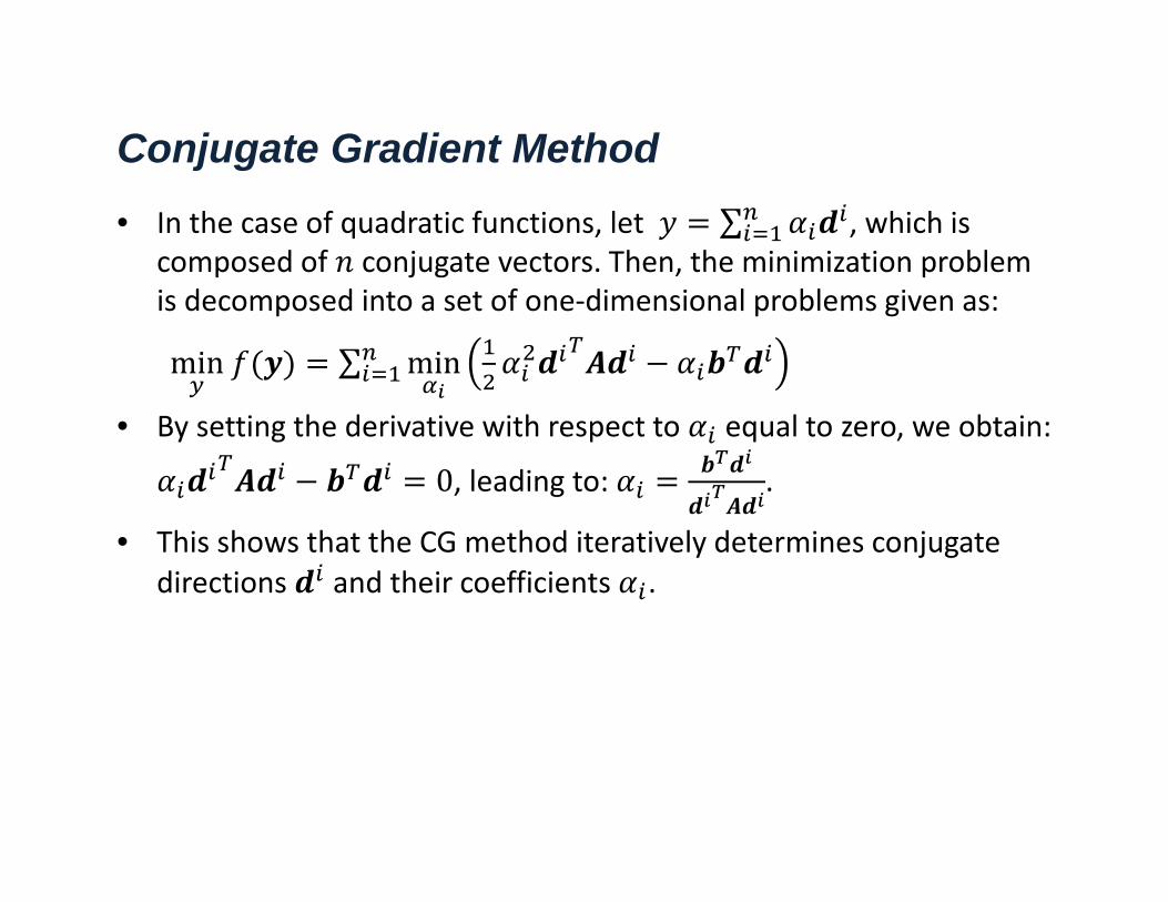
Conjugate Gradient Method• In the case of quadratic functions, let   ∑ , which is 

composed of  conjugate vectors. Then, the minimization problem is decomposed into a set of one‐dimensional problems given as:

min ∑ min

• By setting the derivative with respect to  equal to zero, we obtain: 

0, leading to:  . 

• This shows that the CG method iteratively determines conjugate directions  and their coefficients  . 

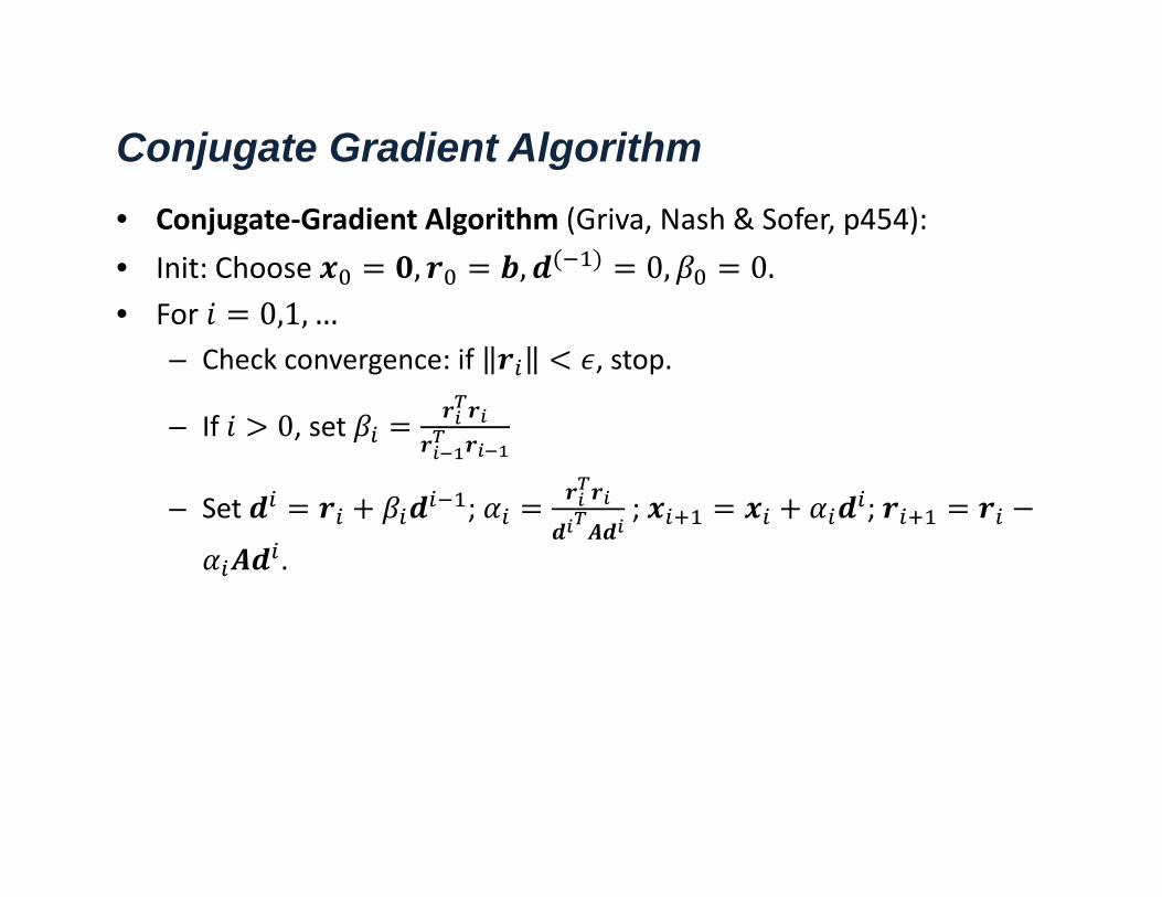
Conjugate Gradient Algorithm • Conjugate‐Gradient Algorithm (Griva, Nash & Sofer, p454):• Init: Choose  , , 0, 0.• For  0,1,…

– Check convergence: if  , stop.

– If  0, set 

– Set  ;  ;  ; 

.

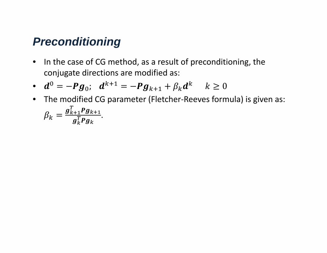
Preconditioning• In the case of CG method, as a result of preconditioning, the 

conjugate directions are modified as:• ; 0• The modified CG parameter (Fletcher‐Reeves formula) is given as: 

.

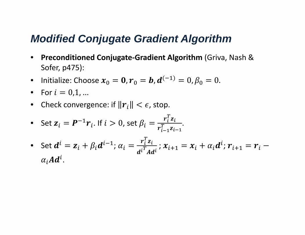
Modified Conjugate Gradient Algorithm• Preconditioned Conjugate‐Gradient Algorithm (Griva, Nash & 

Sofer, p475):• Initialize: Choose  , , 0, 0.• For  0,1,…• Check convergence: if  , stop.

• Set  . If  0, set  .

• Set  ;  ;  ; 

.

CG Rate of Convergence• Conjugate gradient methods achieve superlinear convergence, 

which degenerates to linear convergence if the initial direction is not chosen as the steepest descent direction. 

• In the case of quadratic functions, the minimum is reached exactly in  iterations. For general nonlinear functions, convergence in 2iterations is to be expected. 

• Nonlinear CG methods typically have the lowest per iteration computational costs of all gradient methods.

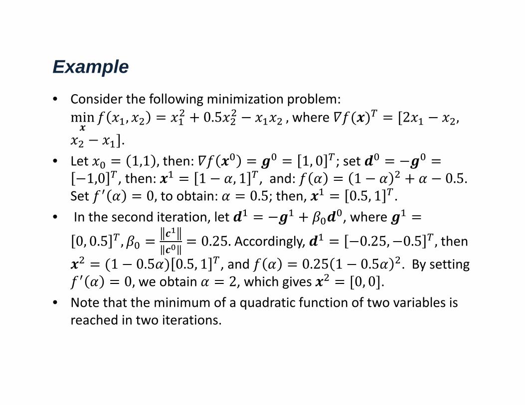
Example • Consider the following minimization problem: min , 0.5 , where  2 ,

. • Let  1,1 , then:  1, 0 ; set 

1,0 , then:  1 , 1 ,  and:  1 0.5. Set  0, to obtain:  0.5; then,  0.5, 1 . 

• In the second iteration, let  , where 

0, 0.5 , 0.25. Accordingly,  0.25, 0.5 ,then 1 0.5 0.5, 1 , and  0.25 1 0.5 .  By setting 0, we obtain  2, which gives  0, 0 . 

• Note that the minimum of a quadratic function of two variables is reached in two iterations.

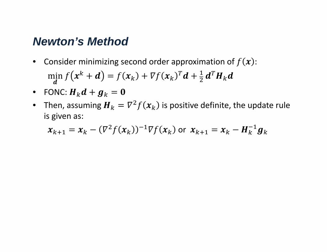
Newton’s Method• Consider minimizing second order approximation of  :

min

• FONC: • Then, assuming  is positive definite, the update rule 

is given as:or  

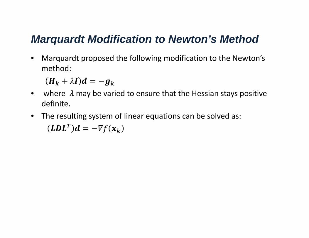
Marquardt Modification to Newton’s Method• Marquardt proposed the following modification to the Newton’s 

method:

• where   may be varied to ensure that the Hessian stays positive definite. 

• The resulting system of linear equations can be solved as:

Modified Newton’s Method• The classical Newton’s method assumes a step size of  1.• A modified Newton’s method is given as:

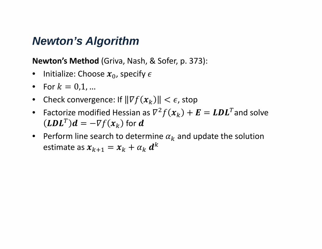
Newton’s AlgorithmNewton’s Method (Griva, Nash, & Sofer, p. 373): • Initialize: Choose  , specify • For  0,1,…• Check convergence: If  , stop• Factorize modified Hessian as  and solve 

for • Perform line search to determine  and update the solution 

estimate as 

Rate of Convergence• Rate of Convergence. Newton’s method achieves quadratic rate of 

convergence in the close neighborhood of the optimal point, and superlinear rate of convergence otherwise. 

• The main drawback of the Newton’s method is its computational cost: the Hessian matrix needs to be computed at every step, and a linear system of equations needs to be solved to obtain the update. 

• Due to its high computational and storage costs, classic Newton’s method is rarely used in practice. 

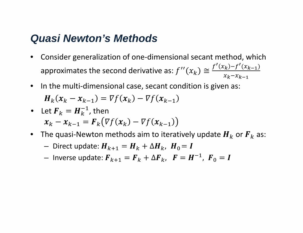
Quasi Newton’s Methods• Consider generalization of one‐dimensional secant method, which 

approximates the second derivative as:  ≅

• In the multi‐dimensional case, secant condition is given as:

• Let  , then 

• The quasi‐Newton methods aim to iteratively update  or  as:– Direct update:  ∆ ,– Inverse update:  ∆ , ,

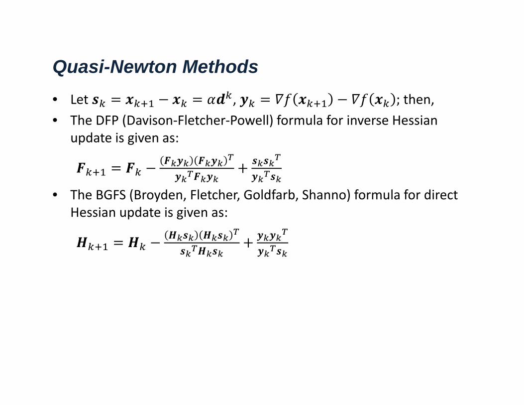
Quasi-Newton Methods• Let  ,  ; then, • The DFP (Davison‐Fletcher‐Powell) formula for inverse Hessian 

update is given as: 

• The BGFS (Broyden, Fletcher, Goldfarb, Shanno) formula for direct Hessian update is given as:

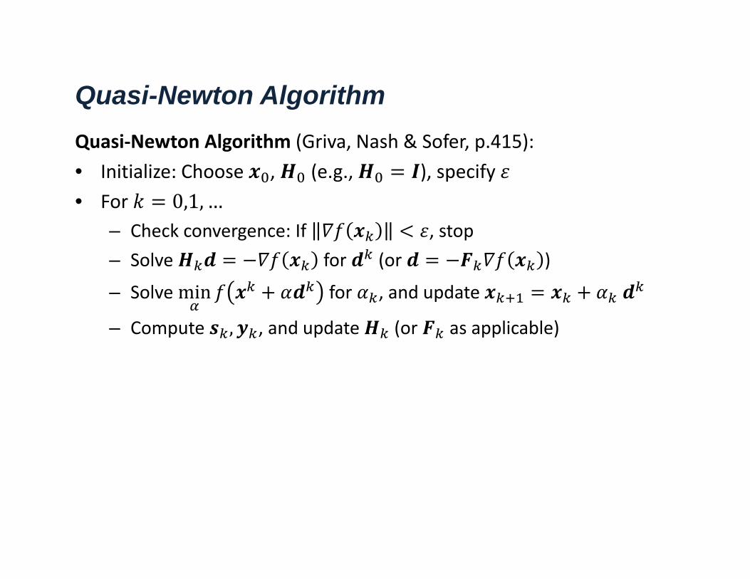
Quasi-Newton AlgorithmQuasi‐Newton Algorithm (Griva, Nash & Sofer, p.415):• Initialize: Choose  ,  (e.g.,  ), specify • For  0,1,…

– Check convergence: If  , stop– Solve  for  (or  )

– Solve min for  , and update 

– Compute  , , and update  (or  as applicable)

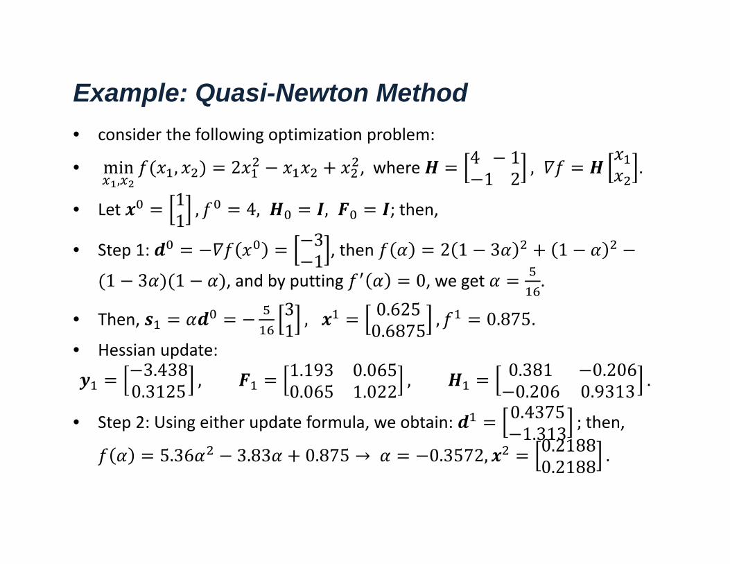
Example: Quasi-Newton Method• consider the following optimization problem: 

• min,

, 2 ,  where  4 112 , .  

• Let  11 , 4, , ; then, 

• Step 1:  31 , then  2 1 3 1

1 3 1 , and by putting  0, we get  . 

• Then,  31 , 0.625

0.6875 , 0.875. • Hessian update: 

3.4380.3125 , 1.193 0.065

0.065 1.022 , 0.381 0.2060.206 0.9313 .

• Step 2: Using either update formula, we obtain:  0.43751.313 ;then, 

5.36 3.83 0.875 → 0.3572, 0.21880.2188 .

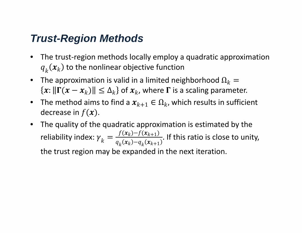
Trust-Region Methods• The trust‐region methods locally employ a quadratic approximation 

to the nonlinear objective function • The approximation is valid in a limited neighborhood Ω

: ∆ of  , where  is a scaling parameter. • The method aims to find a  1 ∈ Ω , which results in sufficient 

decrease in  . • The quality of the quadratic approximation is estimated by the 

reliability index:  1

1. If this ratio is close to unity, 

the trust region may be expanded in the next iteration.

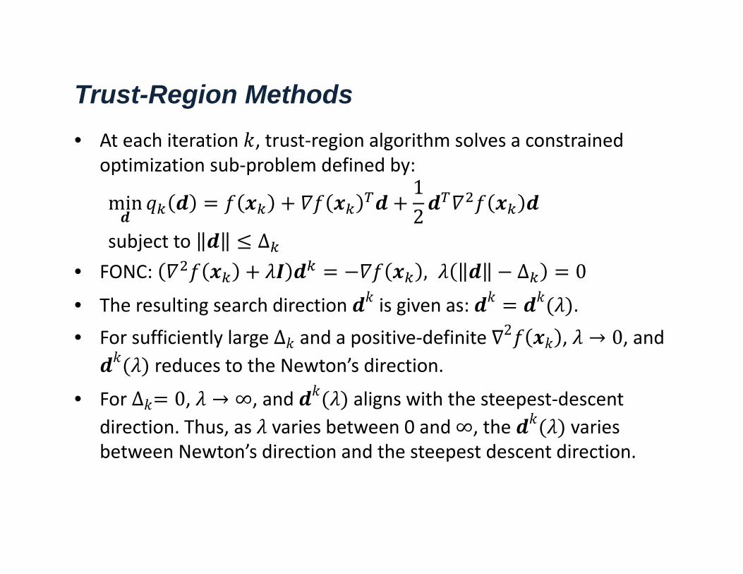
Trust-Region Methods• At each iteration  , trust‐region algorithm solves a constrained 

optimization sub‐problem defined by: 

min12

subject to  ∆• FONC:  , ∆ 0• The resulting search direction  is given as:  . • For sufficiently large∆ and a positive‐definite  2 ,  → 0, and 

reduces to the Newton’s direction. 

• For ∆ 0,  → ∞, and  aligns with the steepest‐descent direction. Thus, as  varies between 0 and ∞, the  varies between Newton’s direction and the steepest descent direction.

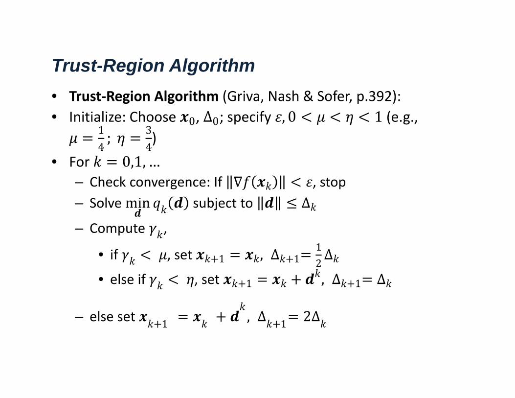
Trust-Region Algorithm• Trust‐Region Algorithm (Griva, Nash & Sofer, p.392):• Initialize: Choose  0, ∆0; specify  , 0 1 (e.g., 

14; 3

4)

• For  0,1,…– Check convergence: If  , stop– Solve min subject to  ∆

– Compute  , 

• if  , set  1 , ∆ 112∆

• else if  , set  1 , ∆ 1 ∆

– else set  1 , ∆ 1 2∆

Computer Methods for Constrained Problems• Penalty and Barrier methods (SUMT)• Augmented Lagrangian method (AL)• Sequential linear programming (SLP)• Sequential quadratic programming (SQP)

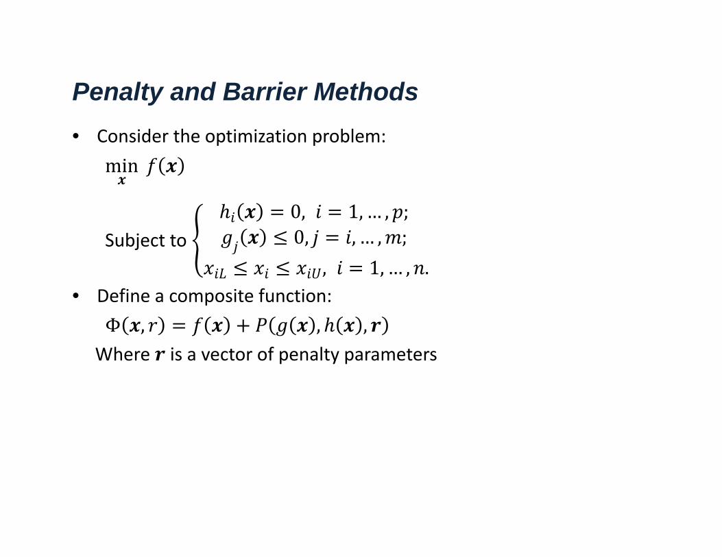
Penalty and Barrier Methods• Consider the optimization problem:

min

Subject to 0, 1,… , ;0, , … , ;

, 1, … , .• Define a composite function:

Φ , , ,Where  is a vector of penalty parameters

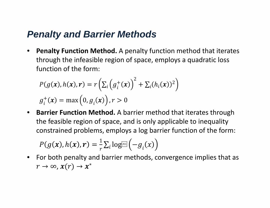
Penalty and Barrier Methods• Penalty Function Method. A penalty function method that iterates 

through the infeasible region of space, employs a quadratic loss function of the form:

, , ∑2

∑ 2

max 0, , 0

• Barrier Function Method. A barrier method that iterates through the feasible region of space, and is only applicable to inequality constrained problems, employs a log barrier function of the form:

, , 1 ∑ log

• For both penalty and barrier methods, convergence implies that as → ∞,  → ∗

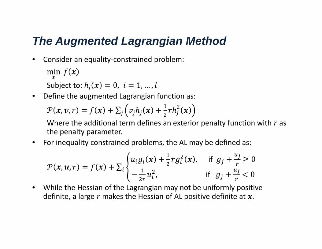
The Augmented Lagrangian Method• Consider an equality‐constrained problem:

min Subject to:  0, 1, … ,

• Define the augmented Lagrangian function as:

, , ∑ 12

2

Where the additional term defines an exterior penalty function with  as the penalty parameter.

• For inequality constrained problems, the AL may be defined as:

, , ∑, if 0

, if 0• While the Hessian of the Lagrangian may not be uniformly positive 

definite, a large  makes the Hessian of AL positive definite at  . 

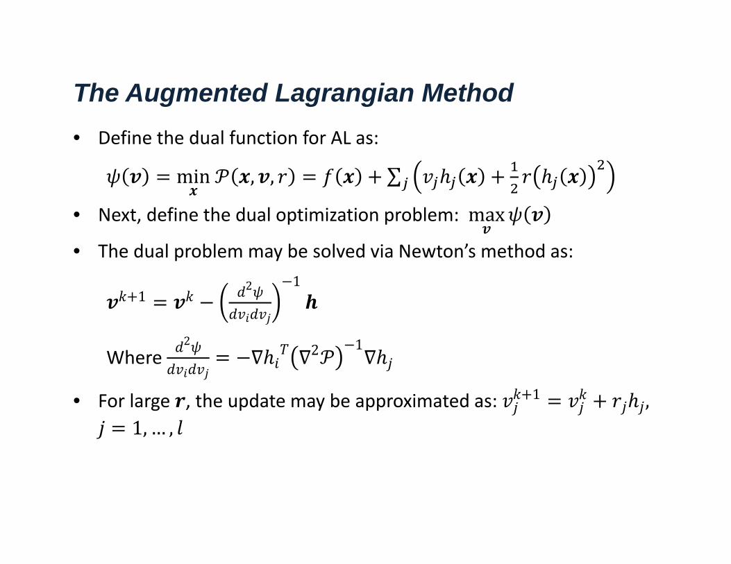
The Augmented Lagrangian Method• Define the dual function for AL as:

min , , ∑

• Next, define the dual optimization problem:  max

• The dual problem may be solved via Newton’s method as:

12 1

Where 2 2 1

• For large  , the update may be approximated as:  1 ,1, … ,

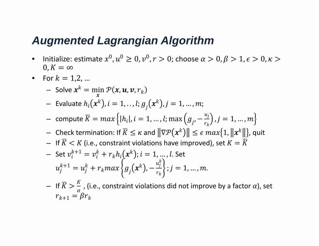
Augmented Lagrangian Algorithm• Initialize: estimate  0, 0 0, 0, 0; choose  0, 1, 0,

0, ∞• For  1,2, …

– Solve  min , , ,

– Evaluate  , 1, . . , ; , 1, … , ;

– compute  , 1, … , ;max , , 1, … ,

– Check termination: If  and  1, , quit– If  (i.e., constraint violations have improved), set  – Set  1 ; 1, … , . Set 

1 , ; 1, … , . 

– If  , (i.e., constraint violations did not improve by a factor  ), set 1

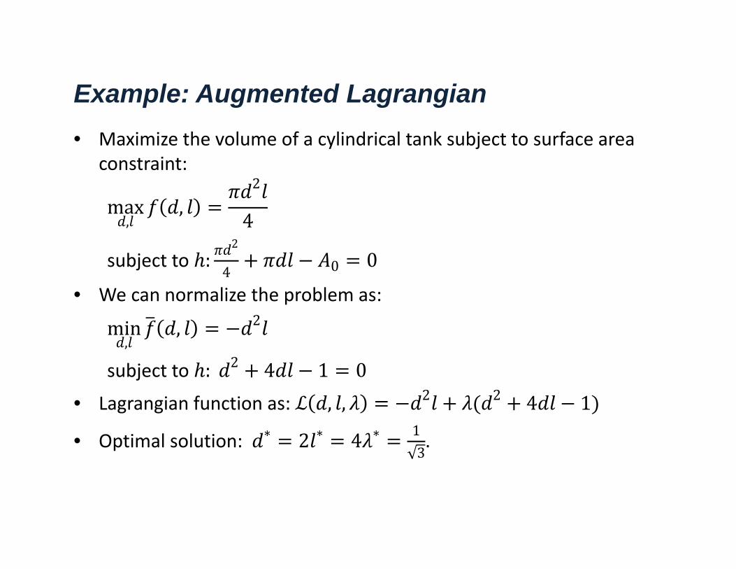
Example: Augmented Lagrangian• Maximize the volume of a cylindrical tank subject to surface area 

constraint:

max,

,2

4

subject to  :2

4 0 0• We can normalize the problem as:

min,

, 2

subject to  : 2 4 1 0• Lagrangian function as:  , , 2 2 4 1

• Optimal solution:  ∗ 2 ∗ 4 ∗ 13.

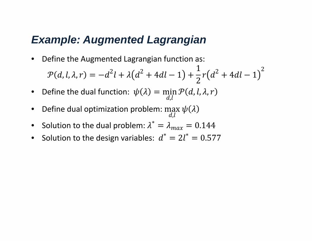
Example: Augmented Lagrangian• Define the Augmented Lagrangian function as:

, , , 2 2 4 112

2 4 12

• Define the dual function:  min,

, , ,

• Define dual optimization problem: max,

• Solution to the dual problem:  ∗ 0.144• Solution to the design variables:  ∗ 2 ∗ 0.577

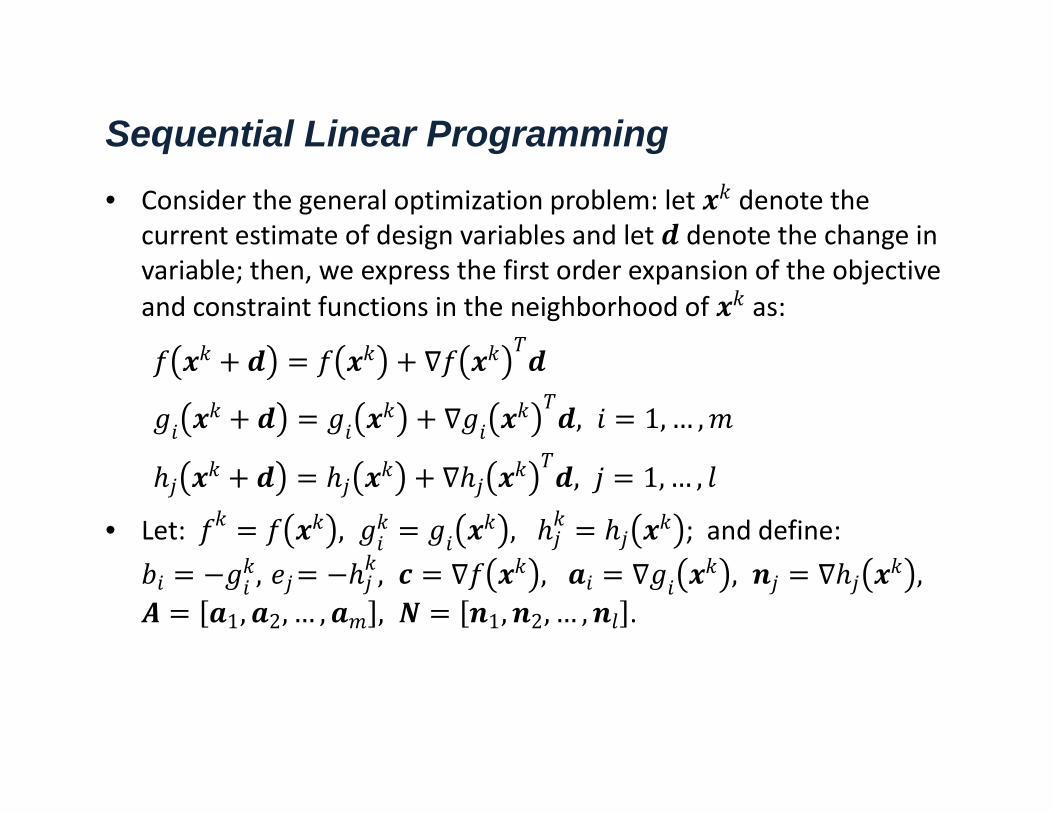
Sequential Linear Programming• Consider the general optimization problem: let  denote the 

current estimate of design variables and let  denote the change in variable; then, we express the first order expansion of the objective and constraint functions in the neighborhood of  as:

, 1, … ,

, 1, … ,

• Let:  , , ;  and define: , , , , ,

1, 2, … , , 1, 2, … , . 

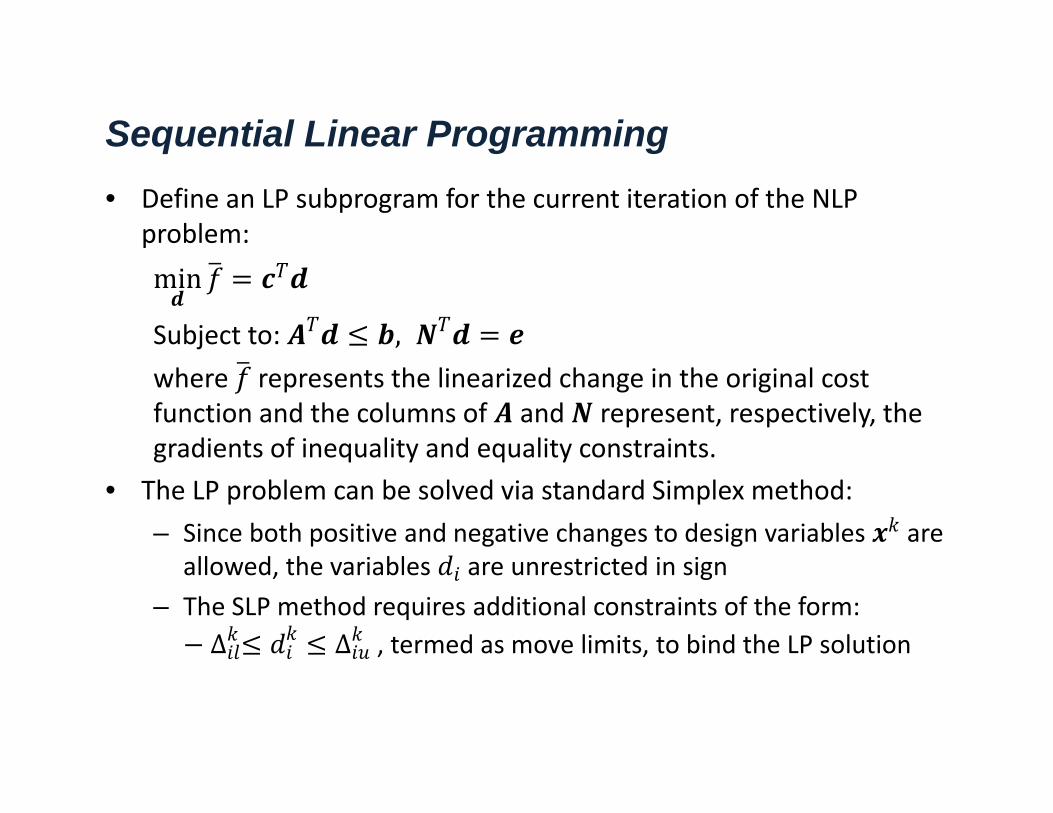
Sequential Linear Programming• Define an LP subprogram for the current iteration of the NLP 

problem:min

Subject to:  ,where  represents the linearized change in the original cost function and the columns of  and  represent, respectively, the gradients of inequality and equality constraints. 

• The LP problem can be solved via standard Simplex method:– Since both positive and negative changes to design variables  are 

allowed, the variables  are unrestricted in sign – The SLP method requires additional constraints of the form: 

∆ ∆ , termed as move limits, to bind the LP solution

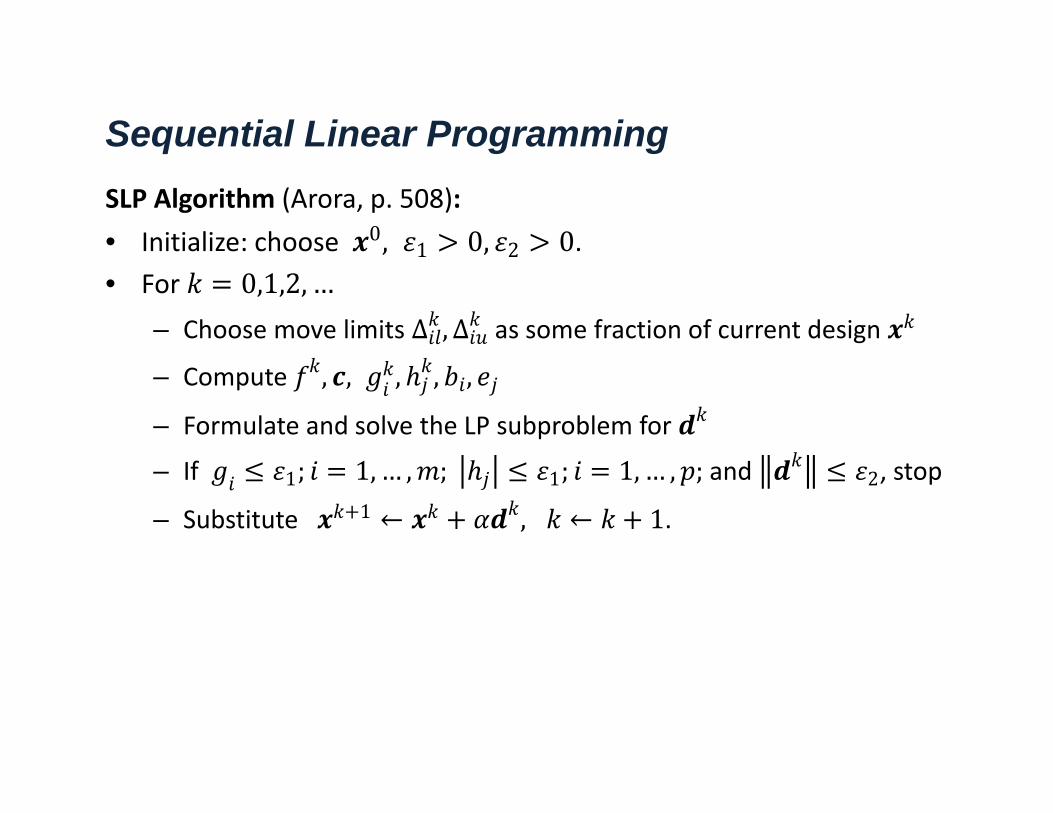
Sequential Linear ProgrammingSLP Algorithm (Arora, p. 508): • Initialize: choose   0, 1 0, 2 0.• For  0,1,2, …

– Choose move limits ∆ , ∆ as some fraction of current design 

– Compute  , , , , ,

– Formulate and solve the LP subproblem for 

– If   1; 1, … , ; 1; 1, … , ; and  2, stop

– Substitute  1 ← , ← 1.

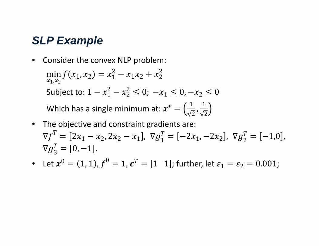
SLP Example• Consider the convex NLP problem:

min1, 2

1, 2 12

1 2 22

Subject to: 1 12

22 0; 1 0, 2 0

Which has a single minimum at:  ∗ 12, 12

• The objective and constraint gradients are:  2 1 2, 2 2 1 , 1 2 1, 2 2 , 2 1,0 ,

3 0, 1 .  

• Let  0 1, 1 , 0 1, 11 ; further, let  1 2 0.001; 

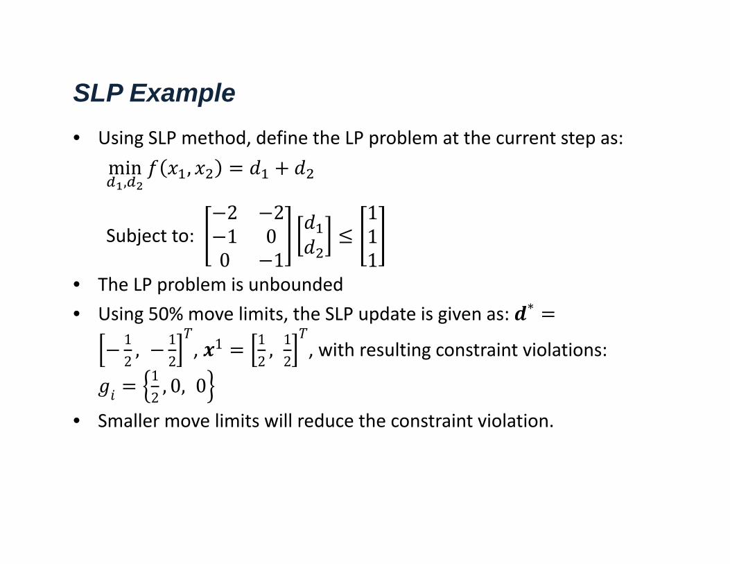
SLP Example• Using SLP method, define the LP problem at the current step as: 

min,

,

Subject to: 2 21 00 1

111

• The LP problem is unbounded• Using 50% move limits, the SLP update is given as:  ∗

12, 1

2,  1 1

2, 12

, with resulting constraint violations: 12, 0, 0

• Smaller move limits will reduce the constraint violation.

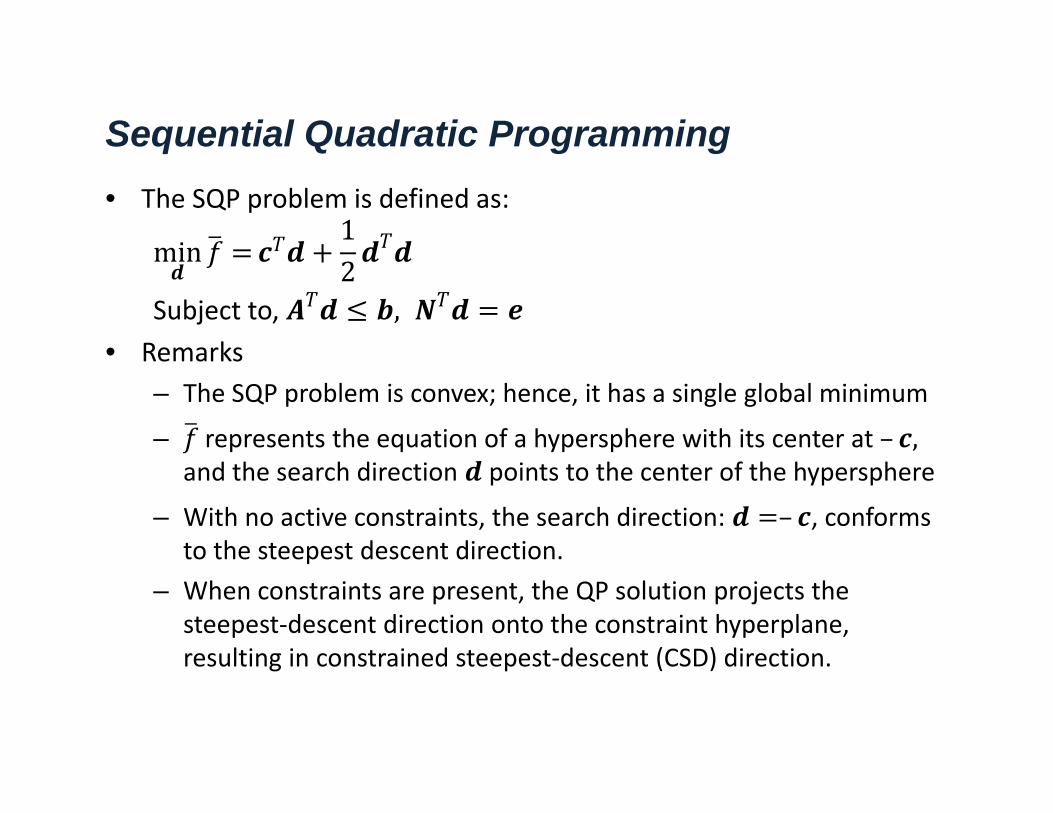
Sequential Quadratic Programming• The SQP problem is defined as:

min12

Subject to,  ,• Remarks

– The SQP problem is convex; hence, it has a single global minimum

– represents the equation of a hypersphere with its center at – ,and the search direction  points to the center of the hypersphere

– With no active constraints, the search direction:  – , conforms to the steepest descent direction. 

– When constraints are present, the QP solution projects the steepest‐descent direction onto the constraint hyperplane, resulting in constrained steepest‐descent (CSD) direction.

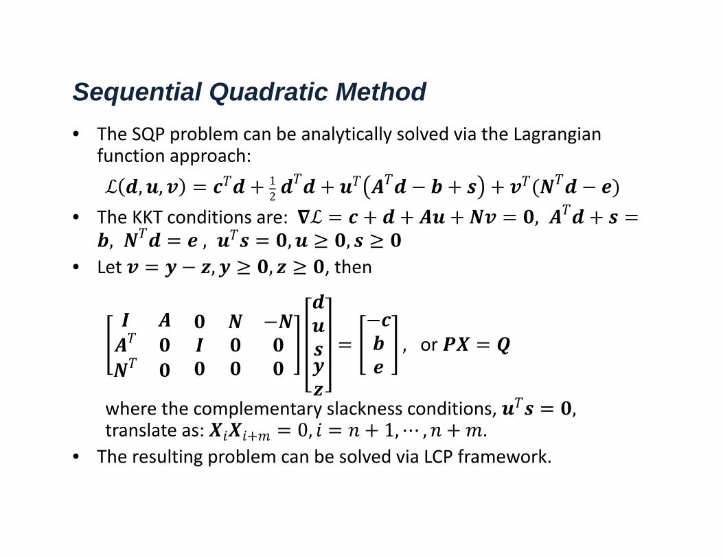
Sequential Quadratic Method• The SQP problem can be analytically solved via the Lagrangian 

function approach:, , 1

2• The KKT conditions are:   ,

, , , ,• Let  , , , then

, or 

where the complementary slackness conditions,  ,translate as:  0, 1,⋯ , . 

• The resulting problem can be solved via LCP framework.

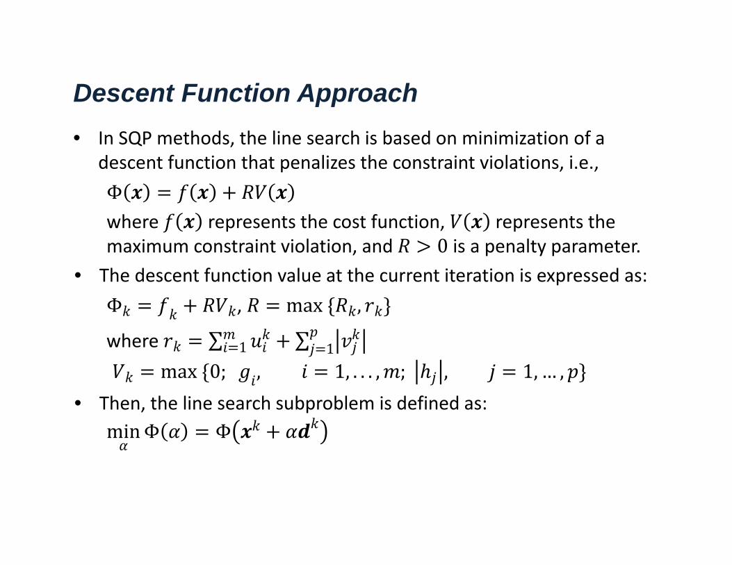
Descent Function Approach • In SQP methods, the line search is based on minimization of a 

descent function that penalizes the constraint violations, i.e., Φwhere  represents the cost function,  represents the maximum constraint violation, and  0 is a penalty parameter. 

• The descent function value at the current iteration is expressed as: Φ ,  max ,

where  ∑ 1 ∑ 1max 0; , 1, . . . , ; , 1, … ,

• Then, the line search subproblem is defined as:minΦ Φ

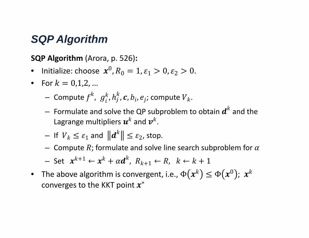
SQP Algorithm SQP Algorithm (Arora, p. 526): • Initialize: choose   0, 0 1, 1 0, 2 0.• For  0,1,2, …

– Compute  , , , , , ; compute  .

– Formulate and solve the QP subproblem to obtain  and the Lagrange multipliers  and  .

– If   1 and   2, stop.– Compute  ; formulate and solve line search subproblem for 

– Set  1 ← , 1 ← , ← 1• The above algorithm is convergent, i.e., Φ Φ 0 ;

converges to the KKT point  ∗

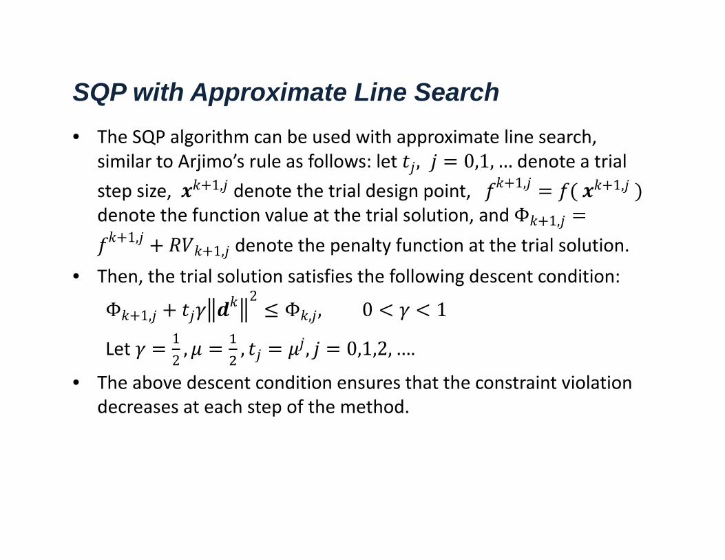
SQP with Approximate Line Search• The SQP algorithm can be used with approximate line search, 

similar to Arjimo’s rule as follows: let  , 0,1, … denote a trial step size,   1, denote the trial design point,    1, 1, denote the function value at the trial solution, and Φ 1,

1,1, denote the penalty function at the trial solution. 

• Then, the trial solution satisfies the following descent condition: 

Φ 1,2

Φ , , 0 1

Let  12, , , 0,1,2, …. 

• The above descent condition ensures that the constraint violation decreases at each step of the method.

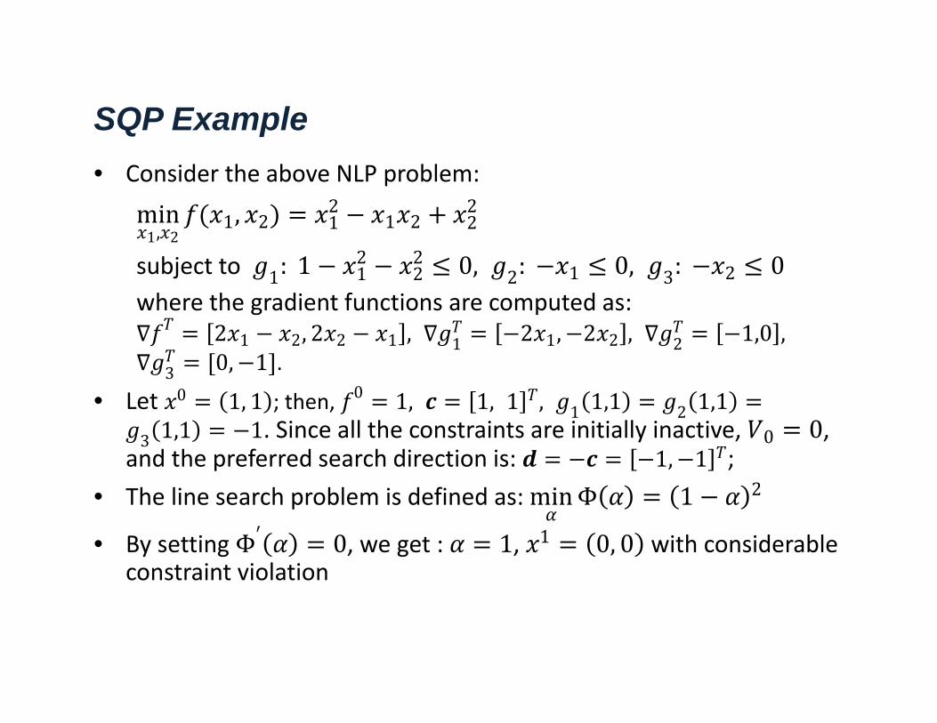
SQP Example• Consider the above NLP problem:

min1, 2

1, 2 12

1 2 22

subject to   1: 1 12

22 0, 2: 1 0, 3: 2 0

where the gradient functions are computed as: 2 1 2, 2 2 1 , 1 2 1, 2 2 , 2 1,0 ,

3 0, 1 .  

• Let  0 1, 1 ; then,  0 1, 1, 1 , 1 1,1 2 1,13 1,1 1. Since all the constraints are initially inactive,  0 0, 

and the preferred search direction is:  1, 1 ; • The line search problem is defined as: minΦ 1 2

• By setting Φ′ 0, we get :  1,  1 0, 0 with considerable constraint violation

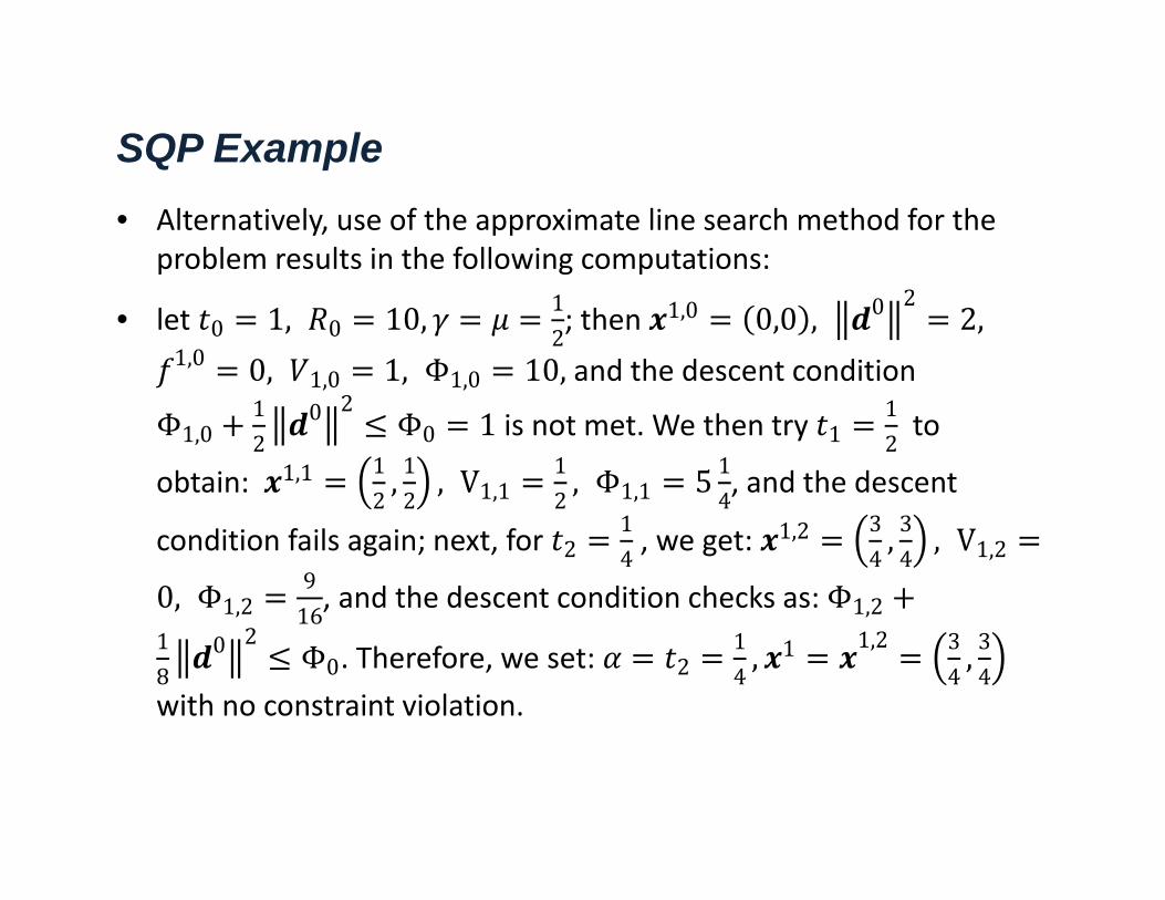
SQP Example• Alternatively, use of the approximate line search method for the 

problem results in the following computations: 

• let  0 1, 0 10, 12; then  1,0 0,0 , 0 2

2,1,0 0, 1,0 1, Φ1,0 10, and the descent condition 

Φ1,012

0 2Φ0 1 is not met. We then try  1

12to 

obtain: 1,1 12, 12, V1,1

12, Φ1,1 5 1

4, and the descent 

condition fails again; next, for  214, we get:  1,2 3

4, 34, V1,2

0, Φ1,2916, and the descent condition checks as: Φ1,2

18

0 2Φ0. Therefore, we set:  2

14, 1 1,2 3

4, 34

with no constraint violation.  

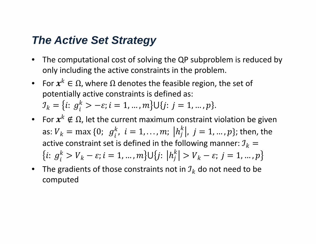
The Active Set Strategy• The computational cost of solving the QP subproblem is reduced by 

only including the active constraints in the problem. • For  ∈ Ω, where Ω denotes the feasible region, the set of 

potentially active constraints is defined as:  : ; 1, … , ⋃ : 1, … , . 

• For  ∉ Ω, let the current maximum constraint violation be given as:  max 0; , 1, . . . , ; , 1, … , ; then, the active constraint set is defined in the following manner: : ; 1, … , ⋃ : ; 1, … ,

• The gradients of those constraints not in  do not need to be computed

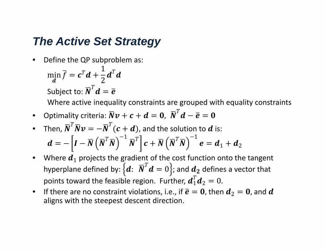
The Active Set Strategy• Define the QP subproblem as:

min12

Subject to: Where active inequality constraints are grouped with equality constraints

• Optimality criteria:  ,• Then,  , and the solution to  is:

1 11 2

• Where  1 projects the gradient of the cost function onto the tangent hyperplane defined by:  : 0 ; and  defines a vector that points toward the feasible region.  Further,  1 2 0.

• If there are no constraint violations, i.e., if  , then  2 , and aligns with the steepest descent direction.

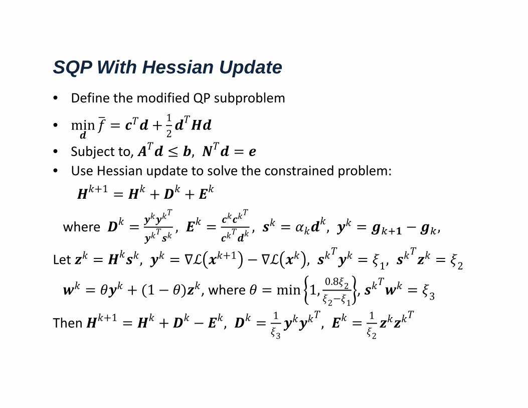
SQP With Hessian Update• Define the modified QP subproblem

• min 12

• Subject to,  ,• Use Hessian update to solve the constrained problem:

1

where   , , , ,

Let  , 1 , 1, 2

1 , where  min 1, 0.8 2

2 1,  3

Then  1 , 1

3, 1

2

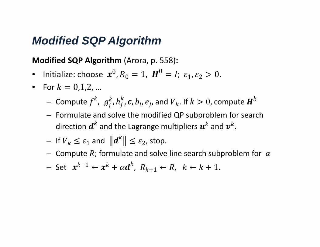
Modified SQP AlgorithmModified SQP Algorithm (Arora, p. 558): 

• Initialize: choose   0, 0 1, 0 ; 1, 2 0.• For  0,1,2, …

– Compute  , , , , , ,and  . If  0, compute – Formulate and solve the modified QP subproblem for search 

direction  and the Lagrange multipliers  and  .

– If  1 and   2, stop.– Compute  ; formulate and solve line search subproblem for  

– Set  1 ← , 1 ← , ← 1.

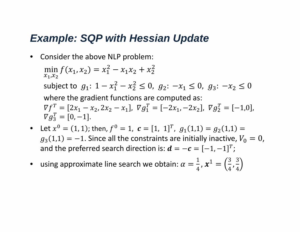
Example: SQP with Hessian Update• Consider the above NLP problem:

min,

,

subject to   : 1 0, : 0, : 0where the gradient functions are computed as: 

2 , 2 , 2 , 2 , 1,0 ,0, 1 .  

• Let  1, 1 ; then,  1, 1, 1 , 1,1 1,11,1 1. Since all the constraints are initially inactive,  0, 

and the preferred search direction is:  1, 1 ;

• using approximate line search we obtain:  14, 1 3

4, 34

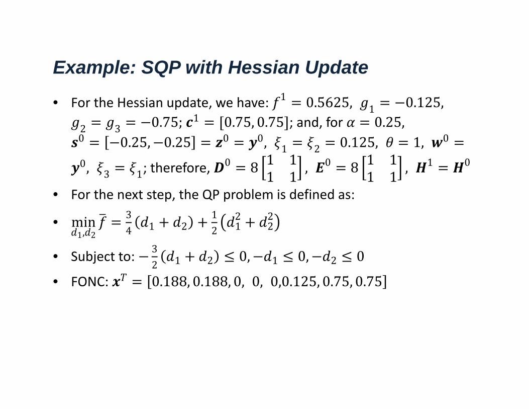
Example: SQP with Hessian Update

• For the Hessian update, we have:  1 0.5625, 1 0.125,

2 3 0.75; 1 0.75, 0.75 ; and, for  0.25,0 0.25, 0.25 0 0, 1 2 0.125, 1, 0

0, 3 1; therefore, 0 8 1 1

1 1 , 0 8 1 11 1 , 1 0

• For the next step, the QP problem is defined as:

• min1, 2

34 1 2

12 1

222

• Subject to:  32 1 2 0, 1 0, 2 0

• FONC:  0.188, 0.188, 0, 0, 0,0.125, 0.75, 0.75