A cooperative conjugate gradient method for linear systems ...
29
HAL Id: hal-01558765 https://hal.inria.fr/hal-01558765 Submitted on 10 Jul 2017 HAL is a multi-disciplinary open access archive for the deposit and dissemination of sci- entific research documents, whether they are pub- lished or not. The documents may come from teaching and research institutions in France or abroad, or from public or private research centers. L’archive ouverte pluridisciplinaire HAL, est destinée au dépôt et à la diffusion de documents scientifiques de niveau recherche, publiés ou non, émanant des établissements d’enseignement et de recherche français ou étrangers, des laboratoires publics ou privés. A cooperative conjugate gradient method for linear systems permitting effcient multi-thread implementation Amit Bhaya, Pierre-Alexandre Bliman, Guilherme Niedu, Fernando Pazos To cite this version: Amit Bhaya, Pierre-Alexandre Bliman, Guilherme Niedu, Fernando Pazos. A cooperative conju- gate gradient method for linear systems permitting effcient multi-thread implementation. Com- putational and Applied Mathematics, Springer Verlag, 2017, pp.1-28. 10.1007/s40314-016-0416-7. hal-01558765
Transcript of A cooperative conjugate gradient method for linear systems ...

HAL Id: hal-01558765https://hal.inria.fr/hal-01558765
Submitted on 10 Jul 2017
HAL is a multi-disciplinary open accessarchive for the deposit and dissemination of sci-entific research documents, whether they are pub-lished or not. The documents may come fromteaching and research institutions in France orabroad, or from public or private research centers.
L’archive ouverte pluridisciplinaire HAL, estdestinée au dépôt et à la diffusion de documentsscientifiques de niveau recherche, publiés ou non,émanant des établissements d’enseignement et derecherche français ou étrangers, des laboratoirespublics ou privés.
A cooperative conjugate gradient method for linearsystems permitting efficient multi-thread
implementationAmit Bhaya, Pierre-Alexandre Bliman, Guilherme Niedu, Fernando Pazos
To cite this version:Amit Bhaya, Pierre-Alexandre Bliman, Guilherme Niedu, Fernando Pazos. A cooperative conju-gate gradient method for linear systems permitting efficient multi-thread implementation. Com-putational and Applied Mathematics, Springer Verlag, 2017, pp.1-28. �10.1007/s40314-016-0416-7�.�hal-01558765�

Computational and Applied Mathematics manuscript No.(will be inserted by the editor)
A cooperative conjugate gradient method for linear
systems permitting efficient multi-thread implementation
Amit Bhaya · Pierre-Alexandre Bliman ·
Guilherme Niedu · Fernando A. Pazos
Received: date / Accepted: date
Abstract This paper revisits, in a multi-thread context, the so-called mul-tiparameter or block conjugate gradient (BCG) methods, first proposed assequential algorithms by O’Leary and Brezinski, for the solution of the linearsystem Ax = b, for an n-dimensional symmetric positive definite matrix A. In-stead of the scalar parameters of the classical CG algorithm, which minimizesa scalar functional at each iteration, multiple descent and conjugate direc-tions are updated simultaneously. Implementation involves the use of multiplethreads and the algorithm is referred to as cooperative CG (CCG) in order toemphasize that each thread now uses information that comes from the otherthreads. It is shown that for a sufficiently large matrix dimension n, the useof an optimal number of threads results in a worst case flop count of O(n7/3)in exact arithmetic. Numerical experiments on a multicore, multi-thread com-puter, for synthetic and real matrices, illustrate the theoretical results.
Keywords Discrete linear systems; Iterative methods; Conjugate gradientalgorithm; Cooperative algorithms;
Mathematics Subject Classification (2000) 65Y05
BhayaDepartment of Electrical Engineering, Federal University of Rio de Janeiro, Rio de Janeiro- RJ, Brazil. E-mail: [email protected]
BlimanSorbonne Universites, Inria, UPMC Univ Paris 06, Lab. J.L. Lions UMR CNRS 7598, Paris,France and Escola de Matematica Aplicada, Fundacao Getulio Vargas, Rio de Janeiro - RJ,Brazil. E-mail: [email protected]
NieduPetrobras, S.A. E-mail: [email protected]
Pazos (corresponding author)Department of Electronics and Telecommunication Engineering, State University of Rio deJaneiro, Rio de Janeiro - RJ, Brazil. Tel.: 55-21-2334-2165 and 55-21-2334-0565. E-mail:[email protected]

2 Amit Bhaya et al.
Funding
A. Bhaya’s work was supported by a BPP grant, G. Niedu and F. Pazos were at UFRJ and
supported by DS and PNPD fellowships, respectively, all of them from National Counsel of
Technological and Scientific Development (CNPq), while this paper was being written.
1 Introduction
The appearance of multi-core processors has motivated much recent interestin multi-thread computation, in which each thread is assigned some part ofa larger computation and executes concurrently with other threads, each onits own core. All threads, however, have relatively fast access to a commonmemory, which is the source and destination of all data manipulated by thethread.
With the availability of ever larger on-chip memory and multicore proces-sors that allow multi-thread programming, it is now possible to propose a newparadigm in which each thread, with access to a common memory, computesits own estimate of the solution to the whole problem (i.e., decompositionof the problem into subproblems is avoided) and the threads exchange infor-mation amongst themselves, this being the cooperative step. The design of acooperative algorithm has the objective of ensuring that exchanged informa-tion is used by the threads in such a way as to reduce overall convergencetime.
The idea of information exchange between two iterative processes was in-troduced into numerical linear algebra, in the context of linear systems, longbefore the advent of multicore processors by Brezinski [10] under the name ofhybrid procedures, defined as (we quote) “a combination of two arbitrary ap-proximate solutions with coefficients summing up to one...(so that) the com-bination only depends on one parameter whose value is chosen in order tominimize the Euclidean norm of the residual vector obtained by the hybridprocedure... The two approximate solutions which are combined in a hybridprocedure are usually obtained by two iterative methods”. The objective ofminimizing the residue is to accelerate convergence of the overall hybrid pro-cedure (also see [2,9]). This idea was generalized and discussed in the contextof distributed asynchronous computation in [6]. It is also worthy of note thatthe paradigm of cooperation between threads, thought of as an independentagents, in order to achieve some common objective, is also becoming popularin many areas such as control [18,22,21].
Several iterative methods to solve the linear algebraic equation
Ax = b (1)
where A ∈ Rn×n is symmetric positive definite and n is large, are well known.
Solving (1) is equivalent to finding the minimizer of the strictly convex scalarfunction
f(x) =1
2xTAx − bTx (2)

Cooperative conjugate gradient method 3
since the unique minimizer of f is x∗ = A−1b.
Conjugate direction methods, based on minimization of (2), can be re-garded as being intermediate between the method of steepest descent andNewton’s method. They are motivated by the desire to accelerate the typ-ically slow convergence associated with steepest descent while avoiding theinformation requirements associated with the evaluation and inversion of theHessian [19, chap. 9].
The conjugate gradient algorithm (CG) is the most popular conjugate di-rection method. It was developed by Hestenes and Stiefel [17]. The algorithmminimizes the scalar function f(x) along conjugate directions searched at eachiteration; the convergence of the sequence of points xk to the solution point x∗
is produced after at most n iterations in exact arithmetic. The residual vectoris defined as
rk = Axk − b (3)
and, given (2), clearly rk = ∇f(xk). In the CG algorithm, the residual vectorrk and a direction vector dk are calculated at the kth iteration,for every k.
O’Leary [23] developed a block CG method (B-CG) in which the conjugatedirections and the residues are taken as columns of n × p matrices. The B-CG algorithm was designed to handle multiple right-hand sides which forma matrix B ∈ R
n×p, but it is also capable of accelerating the convergence oflinear systems with a single right-hand side, for example for solving systemsin which several eigenvalues are widely separated from the others. Severalproperties observed by the vectors in the CG algorithm continue to be valid forthe matrices used in the B-CG algorithm, e.g. the conjugacy property betweenthe matrix directions. Also, in exact arithmetic, the convergence of the B-CGalgorithm to the solution matrix X∗ occurs after at most ⌈n
p ⌉ iterations, which
may involve less work than applying the CG algorithm p times. Gutknecht [16]also analyzes block methods based on Krylov subspaces with multiple righthand sides.
Brezinski ([8, sec. 4] and [3]) developed a block CG algorithm called “multi-parameter CG” (MPCG), which is essentially the B-CG with a single right-hand side b and a single initial point x0. The authors of [8,3] build on thepioneering work of [23], and provide some additional properties, particularlyabout its convergence. It should be noted that the B-CG algorithm as well asthe MPCG algorithm were proposed in the context of a single processor, soissues of multiprocessor implementation, speed up and flop counts were notconsidered in [23,8,3].
This paper revisits Brezinski’s MPCG algorithm from a multi-thread per-spective, calling it, in order to emphasize the new context, the CooperativeConjugate Gradient (CCG) algorithm. The cooperation between threads re-sides in the fact that each thread now uses information that comes from theother threads, and, in addition, the descent and conjugate directions are up-dated simultaneously. The multi-thread implementation of the CCG algorithmaims to accelerate the time to convergence with respect to the B-CG and theMPCG algorithms. Preliminary versions of this paper are [5,4].

4 Amit Bhaya et al.
In [13,14], Gu, Liu et al present a multithread CG method named “multi-ple search direction conjugate gradient method” (MSD-CG), and its precondi-tioned version (PMSD-CG). The method is midway between the CG methodand the Block Jacobi method. It is based on a notion of subdomains or par-titioning of the unknowns. In each iteration there is one search direction persubdomain that is zero in the vector elements that are associated with othersubdomains [13, p. 1134]. The algorithm can be executed in parallel by a mul-ticore processor. The problem is divided into smaller blocks, thus dividing thedirection vectors and the residual vectors into smaller vectors to be calculatedby each processor separately.
This paper is organized as follows. In section 2 the conjugate gradientalgorithm, as well as some basic properties of the conjugate directions are pre-sented. In section 3 the cooperative conjugate gradient algorithm in a multi-thread context is presented. Their basic properties and the convergence rateare studied. In section 4, the computational complexity of the CCG algorithm,as well as the classic CG, the MPCG, and the MSD-CG are investigated. Insection 5 experimental results are presented. In section 6 some general conclu-sions are mentioned. Finally, an appendix presents the proofs of theorems andlemmas.
2 Preliminaries on the classical CG algorithm
This section recalls basic results on the classical CG algorithm in order tomotivate the presentation of the corresponding results for the cooperative CGalgorithm. The reader is referred to [19,15] for all proofs and further detailson the CG algorithm.
Definition 1 Given a symmetric positive definite matrix A, two nonzero vec-tors d1 and d2 are said to be A-orthogonal, or A-conjugate, if dT
1Ad2 = 0.
Lemma 1 If a set of nonzero vectors {d0, . . . ,dk} are A-conjugate (with res-pect to a positive definite matrix A), then these vectors are linearly indepen-dent. The solution x∗ ∈ R
n of the system Ax = b can be expressed as a linearcombination of n A-conjugate vectors {d0, . . . ,dn−1}.
x∗ = α0d0 + · · · + αn−1dn−1
where αi =d
Ti b
dTiAdi
for all i ∈ {0, . . . , n − 1}.
Theorem 1 Let {d0, . . . ,dn−1} be a set of n A-conjugate nonzero vectors.For any x0 ∈ R
n, the sequence generated according to
xk+1 = xk + αkdk (4)
with
αk = − rT
kdk
dT
kAdk(5)
where rk = ∇f(xk) = Axk − b, converges to the unique solution of Ax = b,x∗ after n steps, that is xn = x∗.

Cooperative conjugate gradient method 5
It is notable that the choice (5) ensures the convergence of the sequence (4) inat most n steps in exact arithmetic, which is known as the finite terminationproperty. However, one of the most interesting and still partially understoodproperty of the CG algorithm is that, even when implemented in finite preci-sion arithmetic, approximate convergence to standard tolerances occurs muchfaster than n iterations [20]. Nevertheless, we will use this “worst case” esti-mate of time to convergence in order to generate flop count estimates of theCCG algorithm in section 4. Another fundamental result, the CCG analogof which is presented as Theorem 4 below, is called the expanding subspacetheorem [19].
Theorem 2 Let Bk the space spanned by the set of nonzero conjugate vectors{d0, . . . ,dk−1}. The point xk calculated by the sequence (4) with the step sizes(5) is the global minimizer of f(x) on the subspace x0 + Bk. Moreover, theresidual vector rk = ∇f(xk) = Axk − b is orthogonal to Bk.
2.1 The Conjugate Gradient algorithm
The Conjugate Gradient method, developed by Hestenes and Stiefel [17],is the particular method of conjugate directions obtained when construct-ing the conjugate directions by Gram-Schmidt orthogonalization, achieved atstep k + 1 on the set of the gradients {r0, . . . , rk}. A key point here is thatthis construction can be carried out iteratively. The conjugate gradient al-gorithm is based on the minimization at each iteration of the scalar func-tion f(x) on conjugate directions which form a basis of the Krylov subspaceKk(A, r0) := span{r0, Ar0, A2r0, . . . ,A
k−1r0}.The algorithm is described as follows. Starting from any x0 ∈ R
n, andchoosing d0 = r0 = Ax0 − b, at each iteration, calculate:
xk+1 = xk + αkdk (6)
αk = − rT
kdk
dT
kAdk(7)
dk+1 = rk+1 + βkdk (8)
βk = −rT
k+1Adk
dT
kAdk(9)
In order to qualify as a conjugate gradient algorithm, the directions dk gene-rated at each step should be A-conjugate, which is confirmed in the followingtheorem.
Theorem 3 (Conjugate Gradient Theorem) The conjugate gradient al-gorithm (6)-(9) is a conjugate direction method. If it does not terminate at thestep k, then:
1. span{r0,Ar0, . . . ;Akr0} = span{r0; . . . ; rk} = span{d0, . . . ,dk}. These
subspaces have dimension k + 1.2. dT
kAdi = 0, ∀i < k.
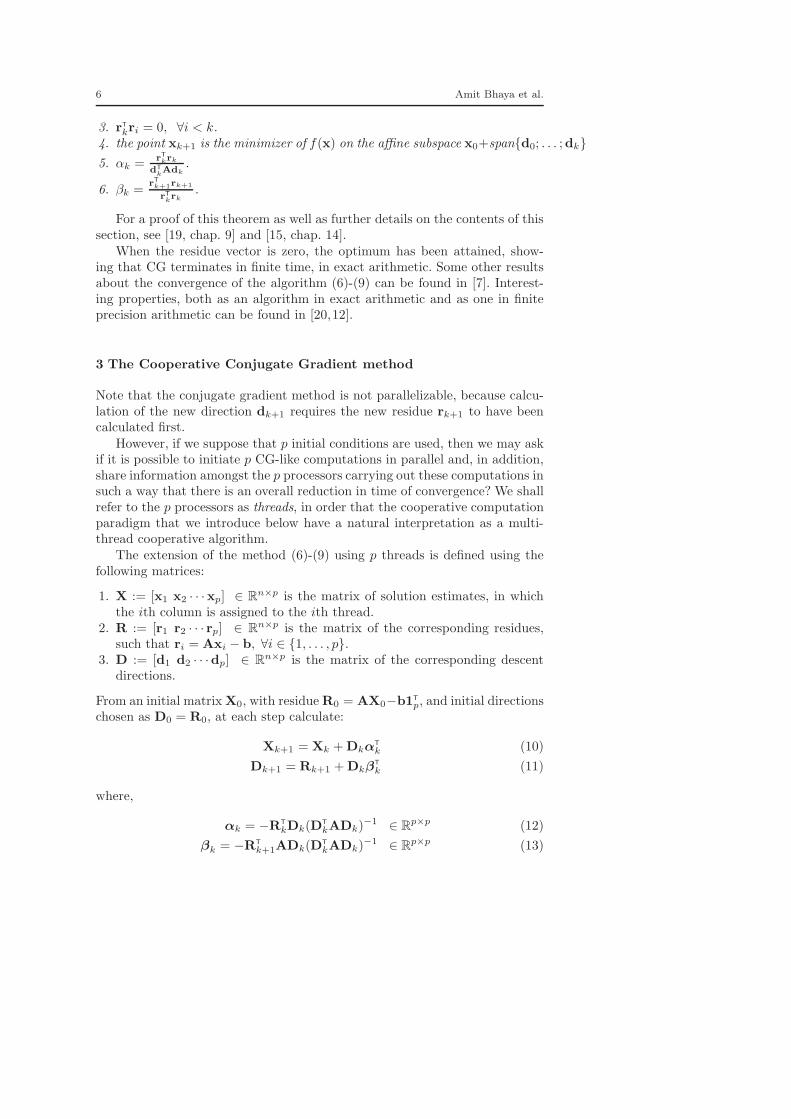
6 Amit Bhaya et al.
3. rT
kri = 0, ∀i < k.4. the point xk+1 is the minimizer of f(x) on the affine subspace x0+span{d0; . . . ;dk}5. αk =
rTkrk
dTkAdk
.
6. βk =r
Tk+1rk+1
rTkrk
.
For a proof of this theorem as well as further details on the contents of thissection, see [19, chap. 9] and [15, chap. 14].
When the residue vector is zero, the optimum has been attained, show-ing that CG terminates in finite time, in exact arithmetic. Some other resultsabout the convergence of the algorithm (6)-(9) can be found in [7]. Interest-ing properties, both as an algorithm in exact arithmetic and as one in finiteprecision arithmetic can be found in [20,12].
3 The Cooperative Conjugate Gradient method
Note that the conjugate gradient method is not parallelizable, because calcu-lation of the new direction dk+1 requires the new residue rk+1 to have beencalculated first.
However, if we suppose that p initial conditions are used, then we may askif it is possible to initiate p CG-like computations in parallel and, in addition,share information amongst the p processors carrying out these computations insuch a way that there is an overall reduction in time of convergence? We shallrefer to the p processors as threads, in order that the cooperative computationparadigm that we introduce below have a natural interpretation as a multi-thread cooperative algorithm.
The extension of the method (6)-(9) using p threads is defined using thefollowing matrices:
1. X := [x1 x2 · · ·xp] ∈ Rn×p is the matrix of solution estimates, in which
the ith column is assigned to the ith thread.2. R := [r1 r2 · · · rp] ∈ R
n×p is the matrix of the corresponding residues,such that ri = Axi − b, ∀i ∈ {1, . . . , p}.
3. D := [d1 d2 · · ·dp] ∈ Rn×p is the matrix of the corresponding descent
directions.
From an initial matrix X0, with residue R0 = AX0−b1T
p, and initial directionschosen as D0 = R0, at each step calculate:
Xk+1 = Xk + DkαT
k (10)
Dk+1 = Rk+1 + DkβT
k (11)
where,
αk = −RT
kDk(DT
kADk)−1 ∈ Rp×p (12)
βk = −RT
k+1ADk(DT
kADk)−1 ∈ Rp×p (13)

Cooperative conjugate gradient method 7
until a stopping criterion (for example ‖ri‖ smaller than a given tolerance forsome i ∈ {1, . . . , p}) is met. In the following, we shall assume that Dk is afull column rank matrix for all iterations k. Note that if p = 1, the method(10)-(13) coincides with (6)-(9).
Remark 1(a) O’Leary [23] considers a block-CG solver which treats multiple right hand
sides at once (B 6= b1T
p). Brezinski ([8, sec. 04] and [3]) considers only onethread x and the initial matrix R0 = D0 is a particular partition of theinitial residue such that R01p = r0 = Ax0 − b.
(b) In section 3.2, the case where p does not necessarily divide n and thecase where rank degeneracy may occur are both analysed: neither case isconsidered in [8,3].
(c) A preconditioned version of a multiparameter CG algorithm (MPCG) waspresented in [11] which proposes a matrix version of the Gram-Schmidtprocess to find the conjugate direction matrices. However, this procedureis very expensive in computational terms. A preconditioned version of theCCG algorithm is not studied here, and will be the object of future research.It is expected that the advantages obtained by preconditioning the classicalCG algorithm will also hold for the CCG algorithm.
3.1 Properties of the cooperative conjugate gradient method
All the relevant results on the CCG algorithm are collected in this subsectionand the next subsection, while the proofs of the key properties are in anappendix, in order for this paper to be complete and self-contained. Lemmas6, 7 and theorems 5, 6 are new, to the best of our knowledge.
In order to present CCG properties that are analogous to those presentedin section 2.1, some notation is introduced. For any set of vectors ri ∈ R
n, i ∈{0, . . . , k}, we denote respectively {ri}k
0 and [ri]k0 the set of these vectors and
the matrix obtained by their concatenation: [ri]k0 = [r0r1 · · · rk] ∈ R
n×(k+1).The notation span [ri]
k0 will denote the subspace of linear combination of the
columns of the matrix [ri]k0 . When R
n is the ambient vector space, we have
span [ri]k0 =
{
v ∈ Rn | ∃γ ∈ R
k+1, v =
k∑
i=0
γiri = [ri]k0γ
}
Similarly, for matrices Ri ∈ Rn×p, i ∈ {0, . . . , k}, we introduce the notations
{Ri}k0 and [Ri]
k0 , which denote, respectively, the set of these matrices and
the matrix obtained as concatenation of the matrices R0,R1, . . . ,Rk, thatis [Ri]
k0 = [R0 R1 · · · Rk] ∈ R
n×p(k+1). Also, we write span [Ri]k0 for the
subspace obtained by all possible linear combinations of the columns of [Ri]k0 :
span [Ri]k0 =
{
v ∈ Rn | ∃γ ∈ R
(k+1)p, v = [Ri]k0γ}

8 Amit Bhaya et al.
Definition 2 Two matrices Q1 and Q2 are called orthogonal if QT
1Q2 = 0,and they are called A-conjugate, or simply conjugate with respect to a matrixA if QT
1AQ2 = 0.
To prove the properties of the algorithm (10)-(13) we first substitute the equa-tion (11) with step size (13) by the direction matrices generated by the Gram-Schmidt process, defined as follows.
The Gram-Schmidt process generates conjugate directions sequentially [15,p. 389]. It can be extended to work with matrices, where every column of amatrix generated by the process in a step is conjugate with respect to everycolumn of the matrices generated in the former steps, in the following way:
Dk+1 = Rk+1 −k∑
j=0
Dj(DT
jADj)−1DT
jARk+1, D0 = R0 (14)
To iterate using (14), it is assumed that all the matrices generated at eachiteration have full column rank (so DT
jADj is nonsingular). It is easy to seethat (14) generates matrices such that DT
jADi = 0 for all i, j ∈ {0, . . . , k+1},i 6= j. As in the classical case, iteration (14) is expensive in computationalterms.
Theorem 4 Let the direction matrices D0, . . . ,Dk be conjugate and of fullcolumn rank. The columns of Xk calculated as in (10), using the step size(12), minimize f(xik
), ∀i ∈ {1, . . . , p} on the affine set xi0 + span [Dj ]k−10 .
Moreover, the columns of Rk are orthogonal to span [Dj ]k−10 , which means
that RT
kDj = 0, ∀j < k.
The next lemma is easy to prove, by induction using (10)-(13), and the factthat Rk+1 = AXk+1 − b1T
p = Rk + ADkαT
k.
Lemma 2 Suppose that D0 = R0, then:
span [R0 R1 · · ·Rk] = span [R0 AR0 · · ·AkR0] = span [D0 D1 · · ·Dk] (15)
Gutknecht [16, sec. 8] defines block-Krylov subspace generated by matricesA ∈ R
n×n and R0 ∈ Rn×p as
K2
k (A,R0) :=
{
X ∈ Rn×p | ∃γ0, · · · , γk ∈ R
p×p, X =
k−1∑
i=0
AiR0γi
}
and a block-Krylov subspace method as an iterative method which generatesmatrices belonging to a block-Krylov subspace Xk ∈ X0 +K2
k (A,R0), at eachiteration.
According to these definitions the method (10) with step size (12) is ablock-Krylov subspace method. Note, however, that the spaces defined in (15)are not block-Krylov subspaces.
Lemma 3 The matrices generated by (14) are the same as those generated by(11) with step size (13).
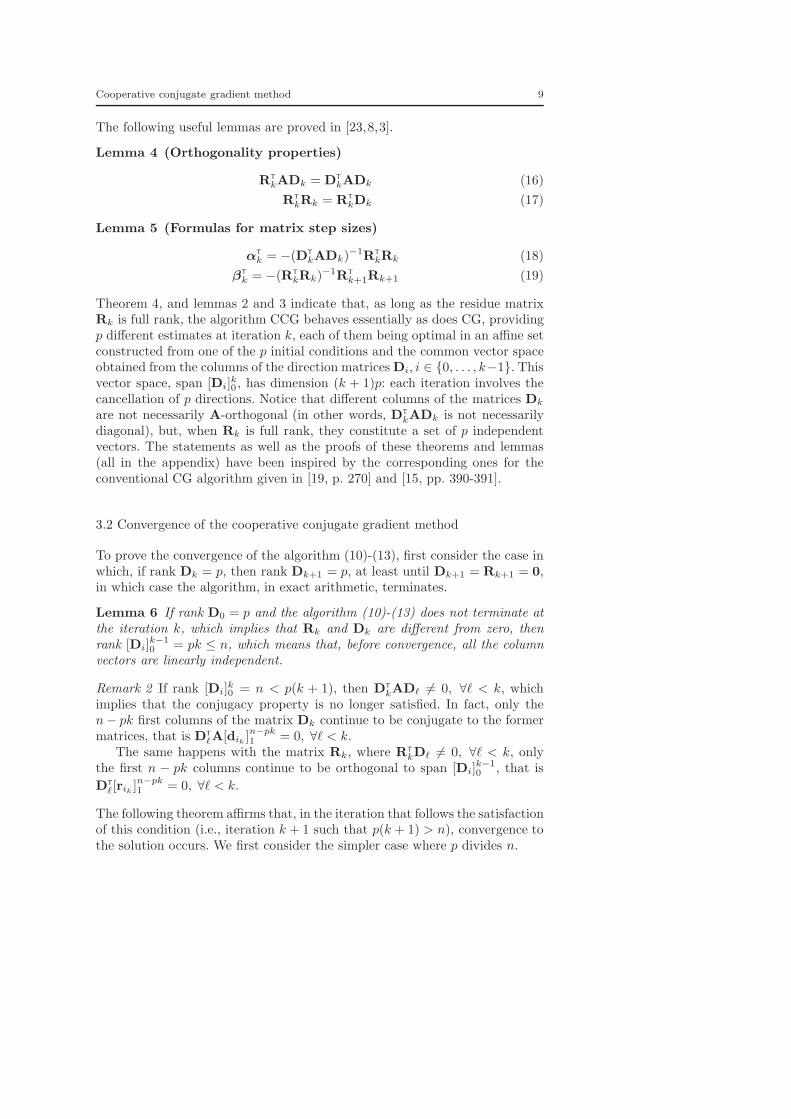
Cooperative conjugate gradient method 9
The following useful lemmas are proved in [23,8,3].
Lemma 4 (Orthogonality properties)
RT
kADk = DT
kADk (16)
RT
kRk = RT
kDk (17)
Lemma 5 (Formulas for matrix step sizes)
αT
k = −(DT
kADk)−1RT
kRk (18)
βT
k = −(RT
kRk)−1RT
k+1Rk+1 (19)
Theorem 4, and lemmas 2 and 3 indicate that, as long as the residue matrixRk is full rank, the algorithm CCG behaves essentially as does CG, providingp different estimates at iteration k, each of them being optimal in an affine setconstructed from one of the p initial conditions and the common vector spaceobtained from the columns of the direction matrices Di, i ∈ {0, . . . , k−1}. Thisvector space, span [Di]
k0 , has dimension (k + 1)p: each iteration involves the
cancellation of p directions. Notice that different columns of the matrices Dk
are not necessarily A-orthogonal (in other words, DT
kADk is not necessarilydiagonal), but, when Rk is full rank, they constitute a set of p independentvectors. The statements as well as the proofs of these theorems and lemmas(all in the appendix) have been inspired by the corresponding ones for theconventional CG algorithm given in [19, p. 270] and [15, pp. 390-391].
3.2 Convergence of the cooperative conjugate gradient method
To prove the convergence of the algorithm (10)-(13), first consider the case inwhich, if rank Dk = p, then rank Dk+1 = p, at least until Dk+1 = Rk+1 = 0,in which case the algorithm, in exact arithmetic, terminates.
Lemma 6 If rank D0 = p and the algorithm (10)-(13) does not terminate atthe iteration k, which implies that Rk and Dk are different from zero, thenrank [Di]
k−10 = pk ≤ n, which means that, before convergence, all the column
vectors are linearly independent.
Remark 2 If rank [Di]k0 = n < p(k + 1), then DT
kADℓ 6= 0, ∀ℓ < k, whichimplies that the conjugacy property is no longer satisfied. In fact, only then− pk first columns of the matrix Dk continue to be conjugate to the formermatrices, that is DT
ℓA[dik]n−pk1 = 0, ∀ℓ < k.
The same happens with the matrix Rk, where RT
kDℓ 6= 0, ∀ℓ < k, onlythe first n − pk columns continue to be orthogonal to span [Di]
k−10 , that is
DT
ℓ[rik]n−pk1 = 0, ∀ℓ < k.
The following theorem affirms that, in the iteration that follows the satisfactionof this condition (i.e., iteration k + 1 such that p(k + 1) > n), convergence tothe solution occurs. We first consider the simpler case where p divides n.

10 Amit Bhaya et al.
Theorem 5 If rank R0 = p, then all of the threads in the cooperative conju-gate gradient method (10)-(13) converge to the solution x∗ in at most k∗ = n
piterations, which means that Rk∗ = Dk∗ = 0 and Xk∗ = x∗1T
p.
Note that lemma 6 indicates that if each matrix Di generated at each iterationhas a rank p, then all the columns of [D0 · · ·Dk] are linearly independent.Unfortunately, even if all columns of the matrices Rk+1 and Dk are linearlyindependent, this does not guarantee that the columns of Dk+1, calculated by(11), also has linearly independent columns.
When the columns of Dk are linearly dependent, it is enough to eliminatecolumns (threads) in such a way that Dk continues to have full column rank,choosing any full-rank subset of columns (so that DT
kADk continues to benonsingular). The linear dependence of the columns of Dk is known as rankdegeneracy (or deflation, which is the term used in [16, sec. 8]). Note that theterm rank degeneracy includes the case when p does not divide n and thuspk∗ > n, as pointed out in remark 2.
O’Leary also considers the possibility of “deleting the zero or redundantcolumn j of Dk and the corresponding columns of Xk and Rk, and continuingthe algorithm with p − 1 vectors... The resulting sequences retain all of theproperties necessary to guarantee convergence” [23, p. 301].
In order to consider the case where rank degeneracy occurs, denote as pk
the number of threads such that rank Dk = pk. We assume p0 = p, and thuspk ≤ p for all k > 0.
Note that the best case is pk = p for all k > 0 until convergence occurs(there is no rank degeneracy). The worst case is pk = 1, ∀k > 0 until conver-gence occurs.
Lemma 7 There exists a finite natural number k∗ such that
mink∗∈N
rank [Di]k∗
−10 = n
The following theorem states conditions for convergence of the CCG algorithmin the general case where rank degeneracy may occur.
Theorem 6 If rank R0 = p > 1, all the threads that converge in the conjugategradient method (10)-(13) converge to x∗ in ⌈n
p ⌉ ≤ k∗ ≤ n − p + 1 iterations,
i.e. xik∗ = x∗ and rik∗ = dik∗ = 0 for all i ∈ {1, . . . , pk∗−1}.
The proof of this theorem is similar to that of theorem 5 for all the threadsthat are not eliminated at any iteration by rank degeneracy, i.e. xik
, ∀i ∈{1, . . . , pk∗−1}. Note that, although rank degeneracy may occur, for all i, j ∈{0, . . . , k∗ − 1}, i 6= j, Di ∈ R
n×pi , Dj ∈ Rn×pj , the conjugacy property
DT
iADj = 0 ∈ Rpi×pj continues to be valid, as well as the orthogonality
property RT
iDj = 0 ∈ Rpi×pj , ∀j < i.
The following lemma, proved in [3, property 11] and [23, theorem 5], givesthe rate of convergence of the CCG algorithm.

Cooperative conjugate gradient method 11
Table 1 Example of the execution of the CCG algorithm with a randomly generated matrixA ∈ R
50×50 from initial conditions that are the columns of a randomly generated matrixX0 ∈ R
50×6, which implies the use of p = 6 threads. The right hand side b is also random.The norm of the residual vector of each thread and the rank of the matrices [Dk] and [Di]k0at each iteration k are reported.
k rank [Dk] rank [Di]k0 ‖r1k
‖ ‖r2k‖ ‖r3k
‖ ‖r4k‖ ‖r5k
‖ ‖r6k‖
0 6 6 3.80 105 4.16 105 3.83 105 3.44 105 3.82 105 3.08 105
1 6 12 1.04 105 0.88 105 1.11 105 1.09 105 0.97 105 0.93 105
2 6 18 4.43 104 4.19 104 4.18 104 3.04 104 3.98 104 4.44 104
3 6 24 1.28 104 2.02 104 2.15 104 1.78 104 1.85 104 2.39 104
4 6 30 5.94 103 8.69 103 7.48 103 12.52 103 14.48 103 10.80 103
5 6 36 3.18 103 3.11 103 4.04 103 5.57 103 6.00 103 4.60 103
6 6 42 1.50 103 2.96 103 3.31 103 3.60 103 2.70 103 4.42 103
7 6 48 1.16 103 4.08 103 3.56 103 4.41 103 2.42 103 5.58 103
8 6 50 252.87 227.31 293.49 250.26 641.00 363.04
9 6 50 1.09 10−4 1.13 10−4 1.43 10−4 1.36 10−4 2.67 10−4 0.45 10−4
Lemma 8 Let κ = λn/λ1 be the condition number of A:
‖xipk− x∗‖A =
2√λ1
p∑
i=1
‖ri0‖(√
κ − 1√κ + 1
)k
(20)
Next, we present an example of the execution of the CCG algorithm for adense randomly generated matrix and using six threads. In this example, norank degeneracy occurs, so that the columns of the matrix [Di]
k0 are linearly
independent until the iteration k∗.
Example 1 Let A ∈ R50×50 be a randomly generated symmetric positive def-
inite matrix, b 6= 0 ∈ R50, and 6 initial conditions X0 ∈ R
50×6 are alsorandomly chosen; thus we have p = 6 threads. Table 1 reports the rank of thematrices [Dk] and [Di]
k0 and the norm of the residual vector of every thread at
each iteration k. Note that in this example the direction vectors are linearlyindependent ([Di]
k0 has full column rank and hence no rank degeneracy oc-
curs). The convergence is produced at an iteration k∗ = 9, where the norm ofthe residual vectors are lower than 10−3.
Brezinski [3, p. 12] affirms that, when pk∗ > n, rank degeneracy always occursin the last iteration, then a “breakdown occurs ... and no general conclusioncan be deduced”. In fact, Algorithm 1 shows pseudocode for the cooperativeconjugate gradient algorithm in the case when rank degeneracy may occur. Inalgorithm 1, X|j∈J refers to the matrix X from which the columns specifiedin the set J have been removed.
4 Estimates of operation counts and speedup of the CCG algorithm
This section estimates the operation counts and speedup of the CCG algo-rithm, when using the CCG algorithm with p threads, instead of CG andMPCG algorithms. The expected speedup is due to the parallelism inherentin a multi-thread implementation. In order to calculate these estimates for

12 Amit Bhaya et al.
Algorithm 1 Pseudocode for the cooperative conjugate gradient algorithm,where X|j∈J refers to the matrix X from which the columns specified in theset J have been removed.1: Choose X0 ∈ R
n×p
2: R0 := AX0 − bT1p
3: D0 := R0
4: p−1 := p5: p0 := rank R0 ⊲ p0 is the initial value of the rank6: k := 07: while pk > 0, do
8: if pk < pk−1 then ⊲ pk−1 − pk threads are suppressed9: choose J ⊂ {1, ., pk−1} such that Dk |j∈J ∈ R
n×pk and rank Dk |j∈J = pk
10: Xk ← Xk |j∈J ⊲ Xk ∈ Rn×pk
11: Rk ← Rk|j∈J ⊲ Rk ∈ Rn×pk
12: Dk ← Dk |j∈J ⊲ Dk ∈ Rn×pk
13: end if
14: αk := −RT
kDk(DT
kADk)−1 ⊲ αk ∈ R
pk×pk
15: Xk+1 := Xk + DkαT
k⊲ Xk+1 ∈ R
n×pk
16: Rk+1 := Rk + ADkαT
k⊲ Rk+1 ∈ R
n×pk
17: βk := −RTk+1ADk(DT
kADk)−1 ⊲ βk ∈ R
pk×pk
18: Dk+1 := Rk+1 + DkβT
k ⊲ Dk+1 ∈ Rn×pk
19: pk+1 := rank Dk+1
20: k ← k + 121: end while
the cooperative conjugate gradient algorithm (10)-(13), we make the followingassumptions:
1. the computations are carried out in exact arithmetic;2. the only floating point operations that are counted are multiplication and
division and both operations take the same amount of time;3. the worst case of finite termination in ⌈n
p ⌉ steps occurs, where n is thedimension of the matrix A;
4. all threads are computationally identical: i.e., all floating point operationsare executed in the same amount of time on each thread,
5. rank degeneracy does not occur, i.e. pk = p for all k ∈ {0, . . . , k∗ − 1}.Rewriting equations (10)-(13) to make the calculations in (10), (11) explicit, weassume that each iteration of the algorithm requires calculating the followingrecursions:
Xk+1 = Xk − Dk(RT
kDk(DT
kADk)−1)T
Rk+1 = Rk − ADk(RT
kDk(DT
kADk)−1)T
Dk+1 = Rk+1 − Dk(RT
k+1ADk(DT
kADk)−1)T
(21)
Table 2, based on the iteration defined in (21), shows the number of floatingpoint operations realized per iteration by each processor in a multi-threadimplementation. Total computation time can be assumed to be proportionalto the total number of floating point operations required to satisfy the stoppingcriterion, neglecting the time spent on communication.
In Table 2, the first column indicates the task carried out at each stageby every thread. The double lines, separating the first row from the second

Cooperative conjugate gradient method 13
Table 2 Operations and corresponding number of floating point operations in the iterationk executed by each processor in a multi-thread implementation
operation result (b) dimension products additions divisions
of proc. i (a) of the result
Adi AD n × p n2 n(n − 1) 0
dTiAD D
TAD p × p np p(n − 1) 0
rTiD R
TD p × p np p(n − 1) 0
αi | αi(DTAD) = r
TiD α := R
TD(DT
AD)−1 p × pp(p+1)(2p+1)
6− p
p(p+1)2
(c)
ri := ri − ADαTi
R := R − ADαT n × p np np 0
xi := xi − DαTi
X := X − DαT n × p np np 0
rTiAD R
TAD p × p np p(n − 1) 0
βi | βi(DTAD) = r
TiAD β := R
TAD(DT
AD)−1 p × pp(p+1)(2p+1)
6− p
p(p+1)2
(c)
di := ri − DβTi
D := R − DβT n × p np np 0
total number of products per iteration n2 + 6np +p(p+1)(2p+1)
3− 2p
total number of additions per iteration n2 − n + 6np +p(p+1)(2p+1)
3− 5p
total number of divisions per iteration p(p + 1)(a) Operation realized by the ith thread, for all i ∈ {1, . . . , p}(b) Composite result of the operations realized by all the p threads at the same time(c) These numbers of floating points operations are needed to realize a Gaussian elimination by LU factorization [25, p. 15]The double line indicates a stage at which communication between all threads occurs, which means that every thread i needsto know results from other threads.
and the second from the third, indicate the necessity of a phase of informationexchange: every thread at that stage needs to know results from other threads.The second column, labelled composite result, contains the information that isavailable by pooling the partial results from each thread and the third columngives the dimension of this composite result. The last three columns containthe number of operations carried out by the ith thread.
As indicated by the last line of Table 2, a total of n2+6np+ p(p+1)(2p+1)3 −2p
multiplications per processor is needed to complete an iteration. In addition,p(p + 1) divisions are carried out per iteration. Since, generically speaking,the algorithm ends in at most n
p iterations, an estimate of the worst-casemultithread execution time is given by the following result.
Theorem 7 (Worst-case multithread CCG flop count) The worst-casemultithread execution of CCG using p agents for a linear system (1) of size nrequires
NCCG(p) =n3
p+ 6n2 +
2
3np2 + 2np− 2
3n (22)
multiplications and divisions carried out in parallel and synchronously, by eachprocessor.
Note that (22) for p = 1 gives the worst-case flop count for the CG algo-rithm:
NCG = NCCG(1) = n3 + 6n2 + 2n (23)
multiplications and divisions.Theorem 7 has the following important corollaries.
Corollary 1 (Multi-thread gain) For problems of size n at least equal to8, it is always beneficial to use p ≤ n processors rather than a single one. In

14 Amit Bhaya et al.
other words, when n ≥ 8,
∀ 1 ≤ p ≤ n, NCCG(1) ≥ NCCG(p) (24)
Proof:
NCCG(1) − NCCG(n) = n3 + 6n2 + 2n −(
23n3 + 9n2 − 2
3n)
= 13 (n3 − 9n2 + 8n)
= 13n(n − 1)(n − 8)
Moreover,dNCCG
dp
∣
∣
∣
∣
p=1
=1
3n(
−3n2 + 10)
which is negative for n ≥ 2, while
dNCCG
dp
∣
∣
∣
∣
p=n
= n
(
4
3n + 1
)
> 0
The convexity of NCCG(p) as a function of p then yields the conclusion thatNCCG(p) ≤ NCCG(1) for any 1 ≤ p ≤ n. ⊓⊔
Corollary 2 (Optimal multi-thread gain for CCG) For any size n ofthe problem, there exists a unique optimal number p∗ of processors minimizingNCCG(p). Moreover, when n → +∞,
p∗ ≈(
3
4
)13
n23 (25a)
NCCG(p∗) ≈(
(
4
3
)13
+2
3
(
3
4
)23
)
n2+ 13 ≈ 1.651n2+1
3 (25b)
Proof:
dNCCG(p)
dp= −n3
p2+
4
3np + 2n
There exists a unique p∗ such that dNCCG/dp = 0. For this value, one hasn2 = (p∗)2(4
3p∗ + 2), which yields the asymptotic behavior given in (25a). Thevalue in (25b) is directly deduced, by substituting (25a) in (22). ⊓⊔
Corollary 1 implies that for n > 8, for every choice of the number of threadsp: NCCG(p) < NCG, and thus the CCG algorithm can be expected to convergein less time than the CG algorithm.
The important conclusion of corollary 2 is that, in the asymptotic limit,as n becomes large, implying that the optimal p∗ also increases according to(25a), solution of Ax = b is possible, by the multi-thread method proposed in
this paper, with a cost of O(n2+ 13 ) floating point operations, showing a clear
advantage over the classical result of O(n3) for Gaussian elimination.

Cooperative conjugate gradient method 15
4.1 Worst-case operation count for other block CG algorithms
The multiparameter conjugate gradient algorithm proposed by Brezinski in [3]and [8, sec. 4], carried out using only one thread, calculates a total number ofscalar products and scalar divisions given by
NMPCG(p) = pNCCG(p) = n3 + 6n2p +2
3np3 + 2np2 − 2
3np (26)
so that with p > 1, NCCG < NMPCG, which means that the CCG algorithmimplemented in a multi-thread context is faster than the MPCG algorithm.The fact that a lower number of iterations than the worst case n/p is expectedin practice does not modify the analysis, because for the same number ofiterations to reach convergence for both the algorithms, the total number offloating point operations executed by the CCG algorithm is always smallerthan those executed by the MPCG algorithm.
We emphasize that, in practice, specially when sparse matrices are used, thenumber of iterations to attain a specified error tolerance is usually much lowerthan ⌈n
p ⌉ and, furthermore, this behavior is also observed with the MPCG and
the B-CG algorithms [20], just as is the case with the classical CG algorithm.The multiple search direction conjugate gradient algorithm (MSD-CG) [13,
14], also implemented in a multi-thread context, performs a number of scalar
products per thread and per iteration equal to n2
p +3np +3n+ p(p+1)(2p+1)
3 −2p;
a number of additions equal to n2
p +3np +n+np+ p(p+1)(2p+1)
3 − 3p− 2, and a
number of scalar divisions equal to p(p + 1). Hence, assuming again that thetime expended to calculate a scalar product is equal to the time expended tocalculate a division, and neglecting the time used to calculate additions, thenumber of floating point operations per iteration performed by the MSD-CGalgorithm is given by:
n2
p+ 3n + 3
n
p+
p(p + 1)(2p + 1)
3+ p(p − 1) (27)
However, it is not proved that the MSD-CG algorithm converges in a finitenumber of iterations [13, p. 1140], and, indeed, this is not expected to occur,essentially because the linear independence of the columns of [Di]
k0 is lost. The
only available result is that the convergence rate is at least as fast as that ofthe steepest descent method [14, p. 1294]. Another drawback of the MSD-CGmethod is that communication between all the threads is required after everyoperation.
5 Computational experiments
This section reports on experimental results obtained with both randomly ge-nerated linear systems of low dimension, as well as larger dimensional matricesthat arise in real applications.

16 Amit Bhaya et al.
Table 3 Properties of randomly generated s.p.d. test matrices: size, condition number
Matrix Dimension Condition no.
A1 50 103
A2 50 104
A3 50 105
B1 100 103
B2 100 104
B3 100 105
C1 200 103
C2 200 104
C3 200 105
D1 300 103
D2 300 104
D3 300 105
E3 1000 105
5.1 Experiments on dense randomly generated matrices of low dimension
For the experiments reported in this section, a suite of randomly generatedsymmetric positive definite matrices of small dimensions will be used for il-lustrative purposes. The dimensions of the matrices are 50, 100, 200, 300 and1000, respectively, and they have condition numbers of 103, 104 and 105. Theright hand side b is also randomly chosen. Table 3 shows the matrix label,its dimension and condition number. In all cases, the CCG algorithm wastested from 20 different initial points per thread (i.e., 20 executions of theCCG algorithm from every initial point per thread). All these initial pointsare localized on a hypersphere of norm 1 centred on the known solution point,that is ‖x0i
− x∗‖ = 1, ∀i ∈ {1, . . . , 20}. The matrices tested, as well as theright hand sides and the initial points are available on request.
The stopping criterion adopted is that at least one thread have a normof its residue smaller than 10−8. We test the CG algorithm (one thread), theCCG algorithm with two and three threads and, for comparative purposes,the MSD-CG algorithm was also implemented.
The 20 initial points tested in the MSD-CG (as well as the CG algorithm)are the same used by the first thread in the CCG algorithm. The partitioninto subdomains of the vector dk which results in the matrix Dk was madeaccording to the criterion given in [13, p. 1136]. Two and three threads weretested. The stopping criterion used was ‖rk‖ < 10−8.
Table 4 reports the mean number of iterations from every initial pointand the mean number of floating point operations (proportional to the timeof convergence, neglecting the communication time and the time expended tocalculate additions) realized in each case.
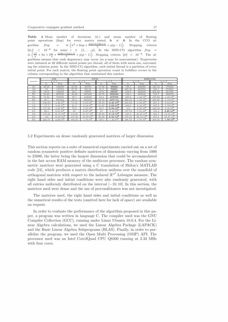
Cooperative conjugate gradient method 17
Table 4 Mean number of iterations (it.) and mean number of floatingpoint operations (flop) for every matrix tested. b 6= 0. In the CCG al-
gorithm flop = it.(
n2 + 6np +p(p+1)(2p+1)
3+ p(p− 1)
)
. Stopping criteria
‖ri‖ < 10−8 for some i ∈ {1, . . . , p}. In the MSD-CG algorithm flop =
it.(
n2
p+ 3n + 3n
p+
p(2p+1)(p+1)3
+ p(p− 1))
. Stopping criteria ‖r‖ < 10−8. The al-
gorithms assume that rank degeneracy may occur (so p may be nonconstant). Trajectorieswere initiated at 20 different initial points per thread, all of them with norm one, surround-ing the solution point. In the MSD-CG algorithm, each initial thread is a partition of everyinitial point. For each matrix, the floating point operation count in boldface occurs in thecolumn corresponding to the algorithm that minimized this number.
CG CCG MSD-CG
matrix p = 1 p = 2 p = 3 p = 2 p = 3it. flop it. flop it. flop it. flop it. flop
A1 48.65 136320 25.95 80750 17.45 59923 159.1 236580 160.15 170930
A2 52 145704 27.35 85113 21.5 73831 405.35 602760 443.1 472940
A3 50.8 142340 32.1 97875 19.9 68337 216.9 322530 235.25 251090
B1 64.85 687540 42.25 507343 33.75 399400 158.1 863540 155.7 586570
B2 74.85 793560 48.7 546020 34.4 407090 263.8 1.44 106 279.85 1.05 106
B3 90.1 955240 90.4 963270 53.75 627110 268.55 1.46 106 300.85 1.13 106
C1 106.95 4.40 106 71.55 3.03 106 56.35 2.45 106 240.05 5.02 106 257.4 3.64 106
C2 117.5 4.84 106 81.2 3.44 106 61.85 2.69 106 402.9 8.42 106 407.9 5.78 106
C3 117.25 4.83 106 79.2 3.35 106 66.7 2.90 106 414 8.65 106 446.35 6.32 106
D1 89.5 8.21 106 67 6.27 106 57 5.44 106 157.75 7.31 106 155.4 4.85 106
D2 179.45 16.47 106 112.95 10.57 106 85.85 8.19 106 437.4 20.27 106 465.7 14.54 106
D3 152 13.95 106 107.85 10.09 106 86.26 8.23 106 576.55 26.73 106 607.5 18.97 106
E3 224.75 2.26 108 168.25 1.70 108 139.7 1.42 108 406.35 2.05 108 409.25 1.38 108
5.2 Experiments on dense randomly generated matrices of larger dimension
This section reports on a suite of numerical experiments carried out on a set ofrandom symmetric positive definite matrices of dimensions varying from 1000to 25000, the latter being the largest dimension that could be accommodatedin the fast access RAM memory of the multicore processor. The random sym-metric matrices were generated using a C translation of Shilon’s MATLABcode [24], which produces a matrix distribution uniform over the manifold of
orthogonal matrices with respect to the induced Rn2
Lebesgue measure. Theright hand sides and initial conditions were also randomly generated, withall entries uniformly distributed on the interval [−10, 10]. In this section, thematrices used were dense and the use of preconditioners was not investigated.
The matrices used, the right hand sides and initial conditions as well asthe numerical results of the tests (omitted here for lack of space) are availableon request.
In order to evaluate the performance of the algorithm proposed in this pa-per, a program was written in language C. The compiler used was the GNUCompiler Collection (GCC), running under Linux Ubuntu 10.0.4. For the Li-near Algebra calculations, we used the Linear Algebra Package (LAPACK)and the Basic Linear Algebra Subprograms (BLAS). Finally, in order to par-allelize the program, we used the Open Multi Processing (OMP) API. Theprocessor used was an Intel Core2Quad CPU Q8200 running at 2.33 MHzwith four cores.

18 Amit Bhaya et al.
0.5 1 1.5 2 2.5
x 104
1000
2000
3000
4000
5000
6000
7000
8000
9000
10000
11000
Matrix dimension
Tim
e (s
)Mean convergence time vs. matrix dimension for the CG and cCG algorithms
Convergence time for CG algorithm
Convergence time for cCG algorithm
CG
CCG
Fig. 1 Mean time to convergence for random test matrices of dimensions varying from 1000to 25000, condition number equal to 106, for 3 thread CCG and standard CG algorithms.
5.2.1 Experimental evaluation of speedup
The results of the cooperative 3 thread CCG, in comparison with standardCG, with a tolerance of 10−3, and matrices with different sizes, but all withthe same condition number of 106, are shown in Figure 1. Multiple tests wereperformed, using different randomly generated initial conditions (20 differentinitial conditions for the small matrices and 10 for the bigger ones). Figure1 shows the mean values computed for these tests. The iteration speedup ofCCG in comparison with CG is defined as the mean number of iterations fromevery initial point that CG took to converge divided by the mean number ofiterations that CCG took to converge, i.e.:
Iteration speedup(p) =mean number of iterations CG
mean number of iterations CCG(p)
Similarly, the time speedup (classical speedup) is the ratio of the time to con-vergence, that is, the mean time taken by the CG algorithm to run the mainloop until convergence divided by the mean time taken by the CCG algorithmfrom every initial point, i.e.:
Time speedup(p) =mean time of convergence CG
mean time of convergence CCG(p)
The experimental speedups for each dimension are shown in Figure 2. Theiteration and classical speedups seem to be roughly equal up to a certain sizeof matrix (n = 16000); however, above this dimension, there is an increasingtrend for both speedups.

Cooperative conjugate gradient method 19
0.5 1 1.5 2 2.5
x 104
1.5
2
2.5
3
3.5
Matrix dimension
Spe
edup
s
Speedups (iteration, time) for cCG versus CG as a function of matrix dimension
Iteration Speedup
Speed−Up TCG
/TcCG
number of CG iterations / number of cCG iterations
Fig. 2 Average speedups of Cooperative 3-thread CCG over classic CG for random testmatrices of dimensions varying from 1000 to 25000, condition number equal to 106.
The numerical results obtained show that CCG, using 3 threads, leads toan improvement in comparison with the usual CG algorithm. The averageiteration speedup and the classical speedup of CCG are respectively, 1.62 and1.94, indicating that CCG converges almost twice as fast as CG for densematrices with reasonably well-separated eigenvalues.
5.2.2 Verifying the flop count estimates
Figure 3 shows the mean time spent per iteration in seconds (points plotted assquares), versus matrix dimension, as well as the parabola fitted to this data,using least squares. Using the result from the last row of table 2 and multi-plying it by the mean time per scalar multiplication, we obtain the parabola(dash-dotted line in Figure 3) expected in theory. In order to estimate the timeper scalar multiplication, we divided the experimentally obtained mean totaltime spent on each iteration and divided it by the number of scalar multipli-cations performed in each iteration. This was done for each matrix dimension.Since the multicore threads being used for all experiments are identical, eachof these divisions should generate the same value of time taken to carry outeach scalar multiplication, regardless of matrix dimension. It was observed thatthese divisions produced a data set which has a mean value of 8.10 nanosecondsper scalar multiplication, with a standard deviation of 1.01 nanoseconds, show-ing that the estimate is reasonable. From equation (22), substituting p = 3,neglecting lower order terms, and multiplying it by the estimated mean timeper scalar multiplication (8.10 nanoseconds), the number of matrix multipli-cations per iteration, NCCG(p), p = 3, is a cubic polynomial in n. Thus, thelogarithm of the dimension (n) of the problem versus the logarithm of timeneeded to convergence is expected to be a straight line of slope 3. Figure 4shows this straight line, fitted to the data (squares) by least squares. Its slope(2.542) is fairly close to 3, and data seems to follow a linear trend. The devia-

20 Amit Bhaya et al.
0.5 1 1.5 2 2.5
x 104
0
0.5
1
1.5
2
2.5
3
3.5
4
4.5
5
Matrix dimension (n) in units of 104
Mea
n tim
e pe
r ite
ratio
n
Mean time per iteration versus matrix dimension
Experimental data
Parabola fitted by least squares
Parabola from worst case theory, Table I
Fig. 3 Mean time per iteration versus problem dimension
7 7.5 8 8.5 9 9.5 100
1
2
3
4
5
6
7
8
Log(Matrix dimension (n))
log(
Tim
e to
con
verg
ence
)
Time to convergence vs.matrix dimension (N)
Experimental data
Least squares fit: y = 2.542*x − 17.658
Fig. 4 Log-log plot of mean time to convergence versus problem dimension
tion of the slope from the ideal value has several probable causes, the first onebeing that the exact exponent of 3 is a result of a worst case analysis of CGin exact arithmetic. It is known that CG usually converges, to a reasonabletolerance, in much less than n iterations [20].
Similarly, the logarithm of the number of iterations needed to convergenceversus the logarithm of the dimension of the problem should also follow alinear trend. Since the number of iterations is expected to be n/3, the slopeof this line should be 1. This log-log plot is shown in figure 5, in which the

Cooperative conjugate gradient method 21
7 7.5 8 8.5 9 9.5 10
5
5.2
5.4
5.6
5.8
6
6.2
6.4
Matrix dimension (n) in units of 103
Itera
tions
nee
ded
to c
onve
rgen
ce
Iterations needed to convergence (with tolerance 10−3) versus matrix dimension
Experimental data points
Fitted curve: y = 0.498*x + 1.376
Fig. 5 Iterations needed to convergence versus problem dimension
straight line was fitted by least squares to the original data (red squares). Theslope (0.501) of the fitted line is smaller than 1, but is seen to fit the data well(small residuals). The fact that both slopes are smaller than their expectedvalues indicates that the CCG algorithm is converging faster than the worstcase estimate. Another reason is that a fairly coarse tolerance of 10−3 is used,and experiments reported show that decreasing the tolerance favors the CCGalgorithm even more.
5.3 Experiments on sparse matrices arising from real applications
In this section the results of tests carried out with a suite of sparse symmetricpositive definite matrices which arise from real applications are reported. Thematrices chosen were taken from [1] and their characteristics are shown inTable 5. The right hand side b was randomly chosen as well as the initialconditions, with all entries uniformly distributed on the interval [−10, 10]. Thetests were performed from 5 different initial points per thread. The stoppingcriterion was that at least one thread has a norm of its residual vector lowerthan 10−8.
The right hand sides used, the initial conditions as well as the numericalresults of the tests are available on request.
The code for the CCG algorithm was written in language C, with compilerGNU Compiler Collection (GCC), running under Linux Ubuntu 10.0.4. Wealso used the Linear Algebra Package (LAPACK) and the Basic Linear AlgebraSubprograms (BLAS). Finally, in order to parallelize the program, we used theOpen Multi Processing (OMP) API. The processor used was an Intel Core i7-4770 3.4 GHz.
The tests were performed varying the number of threads from 1 (classicalCG) to 8 and reporting the mean number of iterations to reach the stopping

22 Amit Bhaya et al.
Table 5 Sparse symmetric positive definite matrices extracted from [1]. Dimension, numberof entries different to zero and approximate condition number. The dash means that thecondition number was not specified or calculated.
name dimension n nonzeros cond. number
HB\bcsstk14 1806 63454 1.31e10HB\bcsstk18 11948 149090 6.486e11
Lourakis\bundle1 10581 770811 1.3306e4TKK\cbuckle 13681 676515 8.0476e7
JGD-Trefethen\Trefethen-20000b 19999 554435 -JGD-Trefethen\Trefethen-20000 20000 554466 -
MathWorks\Kuu 7102 340200 3.2553e4Pothen\bodyy4 17546 121550 1.016e3Pothen\bodyy5 18589 128853 9.9769e3Pothen\bodyy6 19366 134208 9.7989e4
UTEP\Dubcova1 16129 253009 2.6247e3HB\gr-30-30 900 7744 377.23
criterion and the mean time of convergence of the 5 executions performed fromeach one of the different initial points.
For illustrative purposes, Figures 6, 7 and 8 show the speedups for a numberof threads varying from 1 to 8 with respect to the classical CG algorithm forthe matrices bcsstk18, cbuckle and gr-30-30, respectively.
Note that if the CCG algorithm and the CG algorithm converge in theworst case, the numbers of iterations to converge are ⌈n
p ⌉ and n, respectively,
and hence for n ≫ p the expected iteration speedup is equal to p (a straightline of slope 1). Similarly, the expected time speedup in the worst case is givenby the time to convergence of the CG algorithm, which is proportional to NCG
given by (23) divided by the time to convergence taken by the CCG algorithm,which is proportional to NCCG(p) given by (22); for large n this expected timespeedup in the worst case is also approximately equal to p.
Expected worst case time speedup =n3 + 6n2 + 2n
n3
p + 6n2 + 23np2 + 2np− 2
3n
Figure 9 shows the iteration speedup and the time speedup for each matrixreported in Table 5 and for each thread tested from 1 to 8. Figure 9 showsthat for all the matrices tested, the greater the number of threads, the greaterthe speedups, exactly as expected when a small number of threads is used andas it happens in the worst case. For some matrices, an increase in the numberof threads does not increase the speedup significantly, as observed with thematrices bodyy4, bodyy5 and bodyy6, whereas with other matrices the increaseof the speedup with the number of threads is much greater. Further researchis needed to explain these results and correlate them to, for example, theeigenvalue distribution of the matrices.
Figure 10 shows the average iteration and average time speedups for the12 matrices reported in Table 5. Figure 10 confirms the trend of speedupincreasing with the number of threads.

Cooperative conjugate gradient method 23
1 2 3 4 5 6 7 81
1.2
1.4
1.6
1.8
2
2.2
2.4
number of threads p
itera
tion
and
time
spee
dups
speedups for the matrix HB\bcsstk18
iteration speeduptime speedup
n=11948
Fig. 6 Iteration speedup and time speedup for the matrix HB\bcsstk18 vs. number ofthreads p.
1 2 3 4 5 6 7 81
1.1
1.2
1.3
1.4
1.5
1.6
1.7
1.8
1.9
number of threads p
itera
tions
and
tim
e sp
eedu
ps
speedups for the matrix TKK\cbuckle
iteration speed uptime speedup
n=13681
Fig. 7 Iteration speedup and time speedup for the matrix TKK\cbuckle vs. number ofthreads p.
6 Conclusions
This paper revisited some existing block and multiparameter CG algorithms inthe new context of multi-thread computing, proposing a cooperative conjugategradient (CCG) method for linear systems with symmetric positive definitecoefficient matrices. This CCG method permits efficient implementation ona multicore computer and experimental results bear out the main theoreticalproperties, namely, that speedups close to the theoretical value of p, when ap-core computer is used, are possible, when the matrix dimension is suitablylarge.

24 Amit Bhaya et al.
1 2 3 4 5 6 7 81
1.2
1.4
1.6
1.8
2
2.2
2.4
2.6
number of threads p
itera
tion
and
time
spee
dups
speedups for the matrix HB\gr−30−30
iteration speeduptime speedup
n=900
Fig. 8 Iteration speedup and time speedup for the matrix HB\gr-30-30 vs. number ofthreads p.
1
1.5
2
2.5
3
3.5
itera
tion
spee
dup
for
each
mat
rixan
d ea
ch n
umbe
r of
thre
ads
iteration speedup for the matrices shown in Table 5
0
bcss
tk14
bcss
tk18
bund
le1
cbuc
kle
Trefe
then
−200
00b
Trefe
then
−200
00 Kuu
body
y4
body
y5
body
y6
Dubco
va1
gr−3
0−30
p=1p=2p=3p=4p=5p=6p=7p=8
1
1.5
2
2.5
3
3.5
4
time
spee
dup
for
each
mat
rix a
nd
each
num
ber
of th
read
stime speedup for the matrices shown in Table 5
bcss
tk14
bcss
tk18
bund
le1
cbuc
kle
Trefe
then
−200
00b
Trefe
then
−200
00 Kuu
body
y4
body
y5
body
y6
Dubco
va1
gr−3
0−30
p=1p=2p=3p=4p=5p=6p=7p=8
Fig. 9 Iteration speedup (left) and time speedup (right) for each matrix reported in Table5 and for each number of threads used by the CCG algorithm.
The experimental results were carried out with dense randomly generatedmatrices as well as with matrices arising from real applications, which aretypically sparse and sometimes ill-conditioned. In all the cases, the increase ofthe speedups with the number of threads was observed, although the resultsare less significant for some matrices than for others, which is a topic requiringfurther investigation.
The comparison with the other multi-thread block CG method presented inthe literature, the MSD-CG [13,14] showed that the CCG algorithm convergesfaster than the MSD-CG (with the same number of threads), in almost all

Cooperative conjugate gradient method 25
1 2 3 4 5 6 7 81
1.2
1.4
1.6
1.8
2
2.2
2.4
number of threads p
aver
age
itera
tion
spee
dup
and
ave
rage
tim
e sp
eed
up
average speedups between the 12 matrices reported in Table 5
Average iteration speedupAverage time speedup
Fig. 10 Average iteration speedup and time speedup for the 12 matrices reported in Table5 vs. number of threads p.
cases. The tests with large matrices, either dense and randomly generated orsparse arising from real applications, show that the CCG algorithm is fasterthan the classic CG and that the speedup increases with the number of threads.
The use of processors with a larger number of threads should also permitfurther exploration of the notable theoretical result of Corollary 2 that, in theasymptotic limit, as n becomes large, implying that the optimal number ofthreads p∗ also increases according to (25a), solution of Ax = b is possible by
the method proposed here with a worst-case cost of O(n2+ 13 ) floating point
operations.
References
1. Sparse matrix collection. Available at http://www.cise.ufl.edu/research/sparse/matrices/(2009)
2. Abkowicz, A., Brezinski, C.: Acceleration properties of the hybrid procedure for solvinglinear systems. Applicationes Mathematicae 4(23), 417–432 (1996)
3. Bantegnies, F., Brezinski, C.: The multiparameter conjugate gradient algorithm. Tech.Report 429, Laboratoire d’Analyse Numerique et d’Optimisation. Universite des Sci-ences et Technologies de Lille, Lille, France (2001)
4. Bhaya, A., Bliman, P.A., Niedu, G., Pazos, F.: A cooperative conjugate gradient methodfor linear systems permitting multithread implementation of low complexity. ArXiv e-prints (2012)
5. Bhaya, A., Bliman, P.A., Niedu, G., Pazos, F.: A cooperative conjugate gradient methodfor linear systems permitting multithread implementation of low complexity. In: Proc.of the 51st IEEE Conference on Decision and Control. Maui, Hawaii, USA (2012)
6. Bhaya, A., Bliman, P.A., Pazos, F.: Cooperative parallel asynchronous computation ofthe solution of symmetric linear systems. In: Proc. of the 49th IEEE Conference onDecision and Control. Atlanta, USA (2010)
7. Bouyouli, R., Meurant, G., Smoch, L., Sadok, H.: New results on the convergence ofthe conjugate gradient method. Numerical Linear Algebra with Applications pp. 1–12(2008)

26 Amit Bhaya et al.
8. Brezinski, C.: Multiparameter descent methods. Linear Algebra and its Applications296, 113–141 (1999)
9. Brezinski, C., Chehab, J.P.: Nonlinear hybrid procedures and fixed point iterations.Numer. Funct. Anal. Optimization 19, 465–487 (1998)
10. Brezinski, C., Redivo-Zaglia, M.: Hybrid procedures for solving linear systems. Nu-merische Mathematik (67), 1–19 (1994)
11. Bridson, R., Greif, C.: A multipreconditioned conjugate gradient algorithm. SIAMJournal Matrix Anal. Appl. 27(4), 1056–1068 (2006)
12. Greenbaum, A.: Iterative methods for solving linear systems. SIAM, Philadelphia (1997)13. Gu, T., Liu, X., Mo, Z., Chi, X.: Multiple search direction conjugate gradient method
1: Methods and their propositions. International Journal of Computer Mathematics81(9), 1133–1143 (2004)
14. Gu, T., Liu, X., Mo, Z., Chi, X.: Multiple search direction conjugate gradient method2: Theory and numerical experiments. International Journal of Computer Mathematics81(10), 1289–1307 (2004)
15. Guler, O.: Foundations of optimization. Graduate texts in mathematics. Springer, NewYork (2010)
16. Gutknecht, M.H.: Block Krylov space methods for linear systems with multiple right-hand sides: an introduction. In: I.D. A.H. Siddiqi, O. Christensen (eds.) Modern Math-ematical Models, Methods and Algorithms for Real World Systems, pp. 420–447. Ana-maya Publishers, New Delhi, India (2007)
17. Hestenes, M.R., Stiefel, E.: Methods of conjugate gradients for solving linear systems.Journal of Research of the National Bureau of Standards 49, 409–436 (1952)
18. Kumar, V., Leonard, N., Morse, A.S. (eds.): 2003 Block Island Workshop on CooperativeControl, Lecture Notes in Control and Information Sciences, vol. 309. Springer (2005)
19. Luenberger, D.G., Ye, Y.: Linear and nonlinear programming, 3 edn. Springer, NewYork (2008)
20. Meurant, G., Strakos, Z.: The Lanczos and conjugate gradient algorithms in finite pre-cision arithmetic. Acta Numerica 15, 471–542 (2006)
21. Murray, R.M.: Recent research in cooperative control of multi-vehicle systems. J. Guid-ance, Control and Dynamics 129(5), 571–583 (2007)
22. Nedic, A., Ozdaglar, A.: Convex Optimization in Signal Processing and Communica-tions, chap. Cooperative Distributed Multi-agent Optimization, pp. 340–386. CambridgeUniversity Press (2010)
23. O’Leary, D.P.: The block conjugate gradient algorithm and related methods. LinearAlgebra with Applications (29), 293–322 (1980)
24. Shilon, O.: RandOrthMat.m: MATLAB code to gener-ate a random n × n orthogonal real matrix (2006).Http://www.mathworks.com/matlabcentral/fileexchange/authors/23951
25. Strang, G.: Linear algebra and its applications. Harcourt Brace Jovanovich, San Diego,California (1988)
Appendix: Proofs of results in sections 3.1 and 3.2
Proof of theorem 4.For all i ∈ {1, . . . , p}, denoting
hi(γi0, γi1
, . . . , γik−1) := f(xi0 + D0γT
i0+ D1γT
i1+ · · ·+ Dk−1γT
ik−1) ∈ R
where γiℓ∈ R
1×p, ℓ ∈ {0, . . . , k− 1} are row vectors; the coefficients γiℓthat minimize the
scalar function f(x) on the affine set xi0 + span [Dj ]k−10 are given by:
∀ℓ < k : ∂hi∂γ iℓ
T= ∇Tf(xi0 + D0γT
i0+ D1γT
i1+ · · ·+ Dk−1γT
ik−1)Dℓ
= (ri0 + AD0γTi0
+ AD1γTi1
+ · · ·+ ADk−1γTik−1
)TDℓ
= rTi0
Dℓ + γiℓDT
ℓADℓ = 0

Cooperative conjugate gradient method 27
which implies that γiℓ= −rT
i0Dℓ(D
T
ℓADℓ)
−1 ∈ R1×p; and considering all the row vectors
i ∈ {1, . . . , p}:γℓ = −RT
0Dℓ(DTℓADℓ)
−1 ∈ Rp×p (28)
For all x ∈ xi0 + span [Dj ]ℓ−10 : x = xi0 + D0δT
0 + · · · + Dℓ−1δTℓ−1, where δj ∈
R1×p, ∀j ∈ {0, . . . , ℓ− 1}. Thus:
∇f(x) = ri0 + AD0δT0 + · · ·+ ADℓ−1δT
ℓ−1, which implies ∇Tf(x)Dℓ = rTi0
Dℓ
and this is valid for all x ∈ xi0 + span [Dj ]ℓ−10 , hence it is valid for xiℓ
= xi0 + D0αTi0
+
· · ·+Dℓ−1αTiℓ−1
, where αTij
is the ith column of the αTj matrix (12) for all j ∈ {0, . . . , ℓ−1}.
Therefore, ∇Tf(xiℓ)Dℓ = rT
iℓDℓ = rT
i0Dℓ, and considering all the row vectors rT
iℓ, i ∈
{1, . . . , p}:RT
ℓDℓ = RT0Dℓ
and substituting in (28):
γℓ = −RT
ℓDℓ(DT
ℓADℓ)−1 = αℓ ∀ℓ < k (29)
which proves that the step size (12) minimizes f(xik) on the affine set xi0 + span [Dj ]
k−10
for all i ∈ {1, . . . , p}.Note also that, by (10) xik
= xi0 + D0αTi0
+ D1αTi1
+ · · ·+ Dk−1αTik−1
, hence, for all
ℓ < k:
∇Tf(xik)Dℓ = ∇Tf(xi0 + D0αT
i0+ D1αT
i1+ · · ·+ Dk−1αT
ik−1)Dℓ =
(ri0 + AD0αTi0
+ AD1αTi1
+ · · ·+ ADk−1αTik−1
)TDℓ = rTik
Dℓ = 0
and considering all the row vectors i ∈ {1, . . . , p}:
RT
kDℓ = 0 ∀ℓ < k (30)
⊓⊔
Proof of lemma 3.By theorem 4, if Rk is orthogonal to span [Di]
k−10 , then this is orthogonal to span [Ri]
k−10 ,
which means that for all j < k: RT
kRj = 0.
By (10): ∀j < k : Xj+1 = Xj + DjαTj hence DjαT
j = Xj+1 −Xj
which implies RTkADjαT
j = RTk(Rj+1 −Rj)
Supposing rank Dj = p, αj is non singular, thus ∀j < k − 1 : RT
kADj = 0
for j = k − 1 : RT
kADk−1αT
k−1 = RT
kRk 6= 0 ⇒ αT
k−1 = (RT
kADk−1)
−1RT
kRk
Using this result in (14):
Dk+1 = Rk+1 −∑k
j=0 Dj(DTjADj)
−1DTjARk+1
= Rk+1 −Dk(DT
kADk)−1DT
kARk+1
= Rk+1 −Dk(RT
k+1ADk(DT
kADk)−1)T = Rk+1 + DkβT
k
(31)
which coincides with (11) with step size (13), thus proving that the matrices generated bythis method are also conjugate. ⊓⊔
Proof of Lemma 6.By induction. Since the columns of D0 are linearly independent by hypotheses, suppos-
ing rank [Di]k−10 = pk, it is enough to prove that the columns of [Di]k0 also are linearly
independent if p(k + 1) ≤ n.By equation (11): Dk+1 = Rk+1 + DkβT
k .
Evidently, {dik}p1 ⊂ span [Di]
k0 . Using the proof of the lemma 3, {rik+1
}p1 ⊂ span [AiR0]k+10 =
span [Di]k+10 and {rik+1
}p1⊂/span [AiR0]ki = span [Di]k0 because Rk+1 is orthogonal to

28 Amit Bhaya et al.
span [Di]k0 . Hence, the columns of Rk+1 can be expressed neither as a linear combinationof [D0 · · ·Dk ], and, from (11), nor as a linear combination of the columns of Dk+1, which
means that the columns of [D0 · · ·DkDk+1] = [Di]k+10 are linearly independent.
Note that this linear independence persists until an iteration k such that p(k + 1) ≥ n,and in this case [Di]k0 ∈ R
n×p(k+1) and rank [Di]k0 = n ≤ p(k + 1). ⊓⊔
Proof of theorem 5.By lemma 6 [D0 · · ·Dk∗−1] ∈ R
n×pk∗, and rank [D0 · · ·Dk∗−1] = n = pk∗. Hence,
every vector x∗ − xi0 , ∀i ∈ {1, . . . , p} can be expressed as a linear combination of a base of
the subspace span [Di]k∗
−10 :
x∗ − xi0 = D0γTi0
+ D1γTi1
+ · · ·+ Dk∗−2γTik∗−2
+ Dk∗−1γTik∗−1
(32)
where γik∈ R
1×p, k ∈ {0, . . . , k∗ − 1} are the coefficients of the linear combination ofx∗ − xi0 .
Thus, for all k ∈ {0, . . . , k∗ − 1}, i ∈ {1, . . . , p}:
DT
kA(x∗ − xi0 ) = DT
kADkγTik∈ R
p ⇒ γTik
= (DT
kADk)−1DT
kA(x∗ − xi0 )
Following the sequence (10), from xi0 to xikfor all i ∈ {1, . . . , p}:
xik− xi0 = D0αT
i0+ D1αT
i1+ · · ·+ Dk−1αT
ik−1
⇒ DTkA(xik
− xi0 ) = 0⇒ DT
kAxik
= DTkAxi0
where lemma 3 was used and αijis the ith row of the αj matrix calculated as in (12).
Substituting in the former equation:
γTik
= (DT
kADk)−1DT
kA(x∗ − xik) = −(DT
kADk)−1DT
krik
and considering all the p rows:
Γ T
k := [γTik
]p1 = −(DT
kADk)−1DT
kRk
which coincides with (12). Hence, the coefficients of the linear combination (32) are the stepsizes αk , and the sequence
xik∗ = xi0 + D0αTi0
+ · · ·+ Dk∗−1αTik∗−1
(33)
for all i ∈ {1, . . . , p} is equal to x∗, thus proving that all the p threads converge in k∗
iterations. ⊓⊔
Proof of lemma 7.By lemma 6, for all k > 0 until convergence, if Dk 6= 0, then {dik
}pk1 ⊂/span [Di]
k−10
and rank [dik]pk1 = pk ≥ 1. Therefore, the matrix [D0 · · ·Dk∗−1], where k∗ is chosen such
that min rank [D0 · · ·Dk∗−1] ≥ n, has a finite number of columns.
Finally we can choose pk∗−1 = n−∑k∗
−2k=0 pk, that is, we eliminate columns of Dk∗−1
in such a way to have a number of columns enough to complete n linearly independent
columns, i.e. rank [Di]k∗
−10 = rank D0 + · · ·+ rank Dk∗−1 = p0 + · · ·+ pk∗−1 = n. ⊓⊔
Note that in the best case pk = p, ∀k ∈ {0, . . . , k∗ − 1}, which implies that k∗ = ⌈np⌉.
In the general case ⌈np⌉ ≤ k∗ ≤ n− p + 1.


![The Conjugate Gradient Method...Conjugate Gradient Algorithm [Conjugate Gradient Iteration] The positive definite linear system Ax = b is solved by the conjugate gradient method.](https://static.fdocuments.net/doc/165x107/5e95c1e7f0d0d02fb330942a/the-conjugate-gradient-method-conjugate-gradient-algorithm-conjugate-gradient.jpg)