ON ERROR ESTIMATION IN THE CONJUGATE GRADIENT METHOD …

Electronic Transactions on Numerical Analysis.Volume 13, pp. 56-80, 2002.Copyright 2002, Kent State University.ISSN 1068-9613.

ETNAKent State University [email protected]

ON ERROR ESTIMATION IN THE CONJUGATE GRADIENT METHOD ANDWHY IT WORKS IN FINITE PRECISION COMPUTATIONS ∗

ZDENEK STRAKOS† AND PETR TICHY∗

Abstract. In their paper published in 1952, Hestenes and Stiefel considered the conjugate gradient (CG) methodan iterative method which terminates in at most n steps if no rounding errors are encountered [24, p. 410]. They alsoproved identities for the A-norm and the Euclidean norm of the error which could justify the stopping criteria [24,Theorems 6:1 and 6:3, p. 416]. The idea of estimating errors in iterative methods, and in the CG method in particular,was independently (of these results) promoted by Golub; the problem was linked to Gauss quadrature and to itsmodifications [7], [8]. A comprehensive summary of this approach was given in [15], [16]. During the last decadeseveral papers developed error bounds algebraically without using Gauss quadrature. However, we have not foundany reference to the corresponding results in [24]. All the existing bounds assume exact arithmetic. Still they seem tobe in a striking agreement with finite precision numerical experiments, though in finite precision computations theyestimate quantities which can be orders of magnitude different from their exact precision counterparts! For the lowerbounds obtained from Gauss quadrature formulas this nontrivial phenomenon was explained, with some limitations,in [17].

In our paper we show that the lower bound for the A-norm of the error based on Gauss quadrature ([15],[17], [16]) is mathematically equivalent to the original formula of Hestenes and Stiefel [24]. We will compareexisting bounds and we will demonstrate necessity of a proper rounding error analysis: we present an example ofthe well-known bound which can fail in finite precision arithmetic. We will analyse the simplest bound based on[24, Theorem 6:1], and prove that it is numerically stable. Though we concentrate mostly on the lower bound for theA-norm of the error, we describe also an estimate for the Euclidean norm of the error based on [24, Theorem 6:3].Our results are illustrated by numerical experiments.

Key words. conjugate gradient method, Gauss quadrature, evaluation of convergence, error bounds, finiteprecision arithmetic, rounding errors, loss of orthogonality.

AMS subject classifications. 15A06, 65F10, 65F25, 65G50.

1. Introduction. Consider a symmetric positive definite matrix A ∈ Rn×n and a right-

hand side vector b ∈ Rn (for simplicity of notation we will assume A, b real; generalization

to complex data will be obvious). This paper investigates numerical estimation of errors initerative methods for solving linear systems

Ax = b.(1.1)

In particular, we focus on the conjugate gradient method (CG) of Hestenes and Stiefel [24]and on the lower estimates of the A-norm (also called the energy norm) of the error, whichhas important meaning in physics and quantum chemistry, and plays a fundamental role inevaluating convergence [1], [2].

Starting with the initial approximation x0, the conjugate gradient approximations aredetermined by the condition

xj ∈ x0 + Kj(A, r0)

‖x− xj‖A = minu∈x0+Kj(A,r0)

‖x− u‖A,(1.2)

i.e. they minimize the A-norm of the error

‖x− xj‖A =((x− xj), A(x− xj)

) 12

∗Received June 7, 2001. Accepted for publication August 18, 2002. Recommended by L. Reichel.†Institute of Computer Science, Academy of Sciences of the Czech Republic, Pod Vodarenskou vezı 2, 182 07

Praha 8, Czech Republic. E-mail: [email protected] and [email protected]. This researchwas supported by the Grant Agency of the Czech Republic under grant No. 201/02/0595.

56


Estimation of the A-norm of the error in CG computations 57

over all methods generating approximations in the manifold x0 + Kj(A, r0). Here

Kj(A, r0) = span{r0, Ar0, . . . Aj−1r0}

is the j-th Krylov subspace generated by A with the initial residual r0, r0 = b − Ax0, andx is the solution of (1.1). The standard implementation of the CG method was given in [24,(3:1a)-(3:1f)]:

Given x0, r0 = b−Ax0, p0 = r0, and for j = 1, 2, . . . , let

γj−1 = (rj−1, rj−1)/(pj−1, Apj−1),

xj = xj−1 + γj−1 pj−1,(1.3)

rj = rj−1 − γj−1Apj−1,

δj = (rj , rj)/(rj−1, rj−1),

pj = rj + δj pj−1.

The residual vectors {r0, r1, . . . , rj−1} form an orthogonal basis and the direction vectors{p0, p1, . . . , pj−1} an A-orthogonal basis of the j-th Krylov subspace Kj(A, r0).

In [24] Hestenes and Stiefel considered CG as an iterative procedure. They presentedrelations [24, (6:1)-(6:3) and (6:5), Theorems 6:1 and 6:3] as justifications of a possible stop-ping criterion for the algorithm. In our notation these relations become

‖x− xj−1‖2A − ‖x− xj‖

2A = γj−1‖rj−1‖

2,(1.4)

‖x− xj‖2A − ‖x− xk‖

2A =

k−1∑

i=j

γi‖ri‖2, 0 ≤ j < k ≤ n,(1.5)

xj = x0 +

j−1∑

l=0

γlpl = x0 +

j−1∑

l=0

‖x− xl‖2A − ‖x− xj‖

2A

‖rl‖2rl,(1.6)

‖x− xj−1‖2 − ‖x− xj‖

2 =‖x− xj−1‖

2A + ‖x− xj‖

2A

µ(pj−1),(1.7)

µ(pj−1) =(pj−1, Apj−1)

‖pj−1‖2.

Please note that (1.5) represents an identity describing the decrease of the A-norm of theerror in terms of quantities available in the algorithm, while (1.7) describes decrease of theEuclidean norm of the error in terms of the A-norm of the error in the given steps.

Hestenes and Stiefel did not give any particular stopping criterion. They emphasized,however, that while the A-norm of the error and the Euclidean norm of the error had todecrease monotonically at each step, the residual norm oscillated and might even increase ineach but the last step. An example of this behaviour was used in [23].

The paper [24] is frequently referenced, but some of its results has not been paid muchattention. Residual norms have been (and still are) commonly used for evaluating conver-gence of CG. The possibility of using (1.4)–(1.7) for constructing a stopping criterion has notbeen, to our knowledge, considered.

An interest in estimating error norms in the CG method reappeared with works of Goluband his collaborators. Using some older results [7], Dahlquist, Golub and Nash [8] relatederror bounds to Gauss quadrature (and to its modifications). The approach presented in thatpaper became a basis for later developments. It is interesting to note that the relationship


58 Zdenek Strakos and Petr Tichy

of the CG method to the Riemann-Stieltjes integral and Gauss quadrature was described indetail in [24, Section 14], but without any link to error estimation. The work of Golub andhis collaborators was independent of [24].

The paper [8] brought also into attention an important issue of rounding errors. The au-thors noted that in order to guarantee the numerical stability of the computed Gauss quadra-ture nodes and weights, the computed basis vectors had to be reorthogonalized. That meansthat the authors of that paper were from the very beginning aware of the fact that roundingerrors might play a significant role in the application of their bounds to practical computa-tions. In the numerical experiments used in [8] the effect of rounding errors were, however,not noticeable. This can be explained using the results by Paige ([33], [34], [35] and [36]).Due to the distribution of eigenvalues of the matrix used in [8] Ritz values do not convergeto the eigenvalues until the last few steps. Before this convergence takes place there is nosignificant loss of orthogonality and the effects of rounding errors are not visible.

Error bounds in iterative methods were intensively studied or used in many later papersand in several books, see, e.g. [9], [10], [12], [15], [17], [16], [11], [21], [28], [29], [30], [4],[6]. Except for [17], effects of rounding errors were not analysed in these publications.

Frommer and Weinberg [13] pointed out the problem of applying exact precision for-mulas to finite precision computations, and proposed to use interval arithmetic for computingverified error bounds. As stated in [13, p. 201], this approach had serious practical limitations.Axelsson and Kaporin [3] considered preconditioned conjugate gradients and presented (1.5)independently of [24]. Their derivation used (global) mutual A-orthogonality among the di-rection vectors pj , j = 0, 1, . . . , n−1. They noticed that the numerical values found from theresulting estimate were identical to those obtained from Gauss quadrature, but did not provethis coincidence. They also noticed the potential difficulty due to rounding errors. They pre-sented an observation that loss of orthogonality did not destroy applicability of their estimate.Calvetti et al. [5] presented several bounds and estimates for the A-norm of the error, andaddressed a problem of cancellation in their computations [5, relation (46)].

In our paper we briefly recall some error estimates published after (and independently of)(1.4)-(1.7) in [24]. For simplicity of our exposition we will concentrate mostly on theA-normof the error ‖x−xj‖A. We will show that the simplest possible estimate for ‖x−xj‖A, whichfollows from the relation (1.4) published in the original paper [24], is mathematically (inexact arithmetic) equivalent to the corresponding bounds developed later. In finite precisionarithmetic, rounding errors in the whole computation, not only in the computation of theconvergence bounds, must be taken into account. We emphasize that rounding error analysisof formulas for computation of the convergence bounds represents in almost all cases a simpleand unimportant part of the problem. Almost all published convergence bounds (includingthose given in [5]) can be computed accurately (i.e. computation of the bounds using givenformulas is not significantly affected by rounding errors). But this does not prove that thesebounds give anything reasonable when they are applied to finite precision CG computations.We will see an example of the accurately computed bound which gives no useful informationabout the convergence of CG in finite precision arithmetic in Section 6.

An example of rounding error analysis for the bounds based on Gauss quadrature waspresented in [17]. The results from [17] rely on the work by Paige and Greenbaum ([36],[19] and [22]). Though [17] gives a strong qualitative justification of the bounds in finiteprecision arithmetic, this justification is applicable only until ‖x − xj‖A reaches the squareroot of the machine precision. Moreover, quantitative expressions for the rounding error termsare very complicated. They contain factors which are not tightly estimated (see [19], [22]).Here we complement the analysis from [17] by substantially stronger results. We prove thatthe simplest possible lower bound for ‖x − xj‖A based on (1.4) works also for numerically



computed quantities till ‖x− xj‖A reaches its ultimate attainable accuracy.The paper is organized as follows. In Section 2 we briefly describe relations between

the CG and Lanczos methods. Using the orthogonality of the residuals, these algorithmsare related to sequences of orthogonal polynomials, where the inner product is defined bya Riemann-Stieltjes integral with some particular distribution function ω(λ). The value ofthe j-th Gauss quadrature approximation to this Riemann-Stieltjes integral for the function1/λ is the complement to the error in the j-th iteration of the CG method measured by‖x − xj‖

2A/‖r0‖

2. In Section 3 we reformulate the result of the Gauss quadrature usingquantities that are at our disposal during the CG iterations. In Section 4 we use the identitiesfrom Section 3 for estimation of the A-norm of the error in the CG method, and we comparethe main existing bounds. Section 5 describes delay of convergence due to rounding errors.Section 6 explains why applying exact precision convergence estimates to finite precision CGcomputations represents a serious problem which must be properly addressed. Though exactprecision CG and finite precision CG can dramatically differ, some exact precision boundsseem to be in good agreement with the finite precision computations. Sections 7–10 explainthis paradox. The individual terms in the identities which the convergence estimates are basedon can be strongly affected by rounding errors. The identities as a whole, however, hold true(with small perturbations) also in finite precision arithmetic. Numerical experiments are pre-sented in Section 11.

When it will be helpful we will use the word “ideally” (or “mathematically”) to refer toa result that would hold using exact arithmetic, and “computationally” or “numerically” to aresult of a finite precision computation.

2. Method of conjugate gradients and Gauss quadrature. For A and r0 the Lanczosmethod [27] generates ideally a sequence of orthonormal vectors v1, v2, . . . via the recurrence

Given v1 = r0/‖r0‖, β1 ≡ 0, and for j = 1, 2, . . . , let

αj = (Avj − βjvj−1, vj),

wj = Avj − αjvj − βjvj−1,(2.1)

βj+1 = ‖wj‖,

vj+1 = wj/βj+1.

Denoting by Vj = [v1, . . . , vj ] the n by j matrix having the Lanczos vectors {v1, . . . , vj} asits columns, and by Tj the symmetric tridiagonal matrix with positive subdiagonal

Tj =

α1 β2

β2 α2. . .

. . .. . . βj

βj αj

(2.2)

the formulas (2.1) are written in the matrix form

AVj = VjTj + βj+1vj+1eTj ,(2.3)

where ej is the j-th column of the n by n identity matrix. Comparing (1.3) with (2.1) gives

vj+1 = (−1)jrj

‖rj‖,(2.4)



and also relations between the recurrence coefficients:

αj =1

γj−1+δj−1

γj−2, δ0 ≡ 0, γ−1 ≡ 1,

βj+1 =

√δj

γj−1.(2.5)

Finally, using the change of variables

xj = x0 + Vj yj ,(2.6)

and the orthogonality relation between rj and the basis {v1, v2, . . . , vj} of Kj(A, r0), we seethat

0 = V Tj rj = V Tj (b−Axj) = V Tj (r0 −AVj yj)

= e1‖r0‖ − V Tj AVj yj = e1‖r0‖ − Tj yj .

Ideally, the CG approximate solution xj can therefore be determined by solving

Tj yj = e1‖r0‖ ,(2.7)

with subsequent using of (2.6).Orthogonality of the CG residuals creates the elegance of the CG method which is repre-

sented by its link to the world of classical orthogonal polynomials. Using (1.3), the j-th errorresp. residual can be written as a polynomial in the matrix A applied to the initial error resp.residual,

x− xj = ϕj(A) (x− x0), rj = ϕj(A) r0, ϕj ∈ Πj ,(2.8)

where Πj denotes the class of polynomials of degree at most j having the property ϕ(0) = 1(that is, the constant term equal to one). Consider the eigendecomposition of the symmetricmatrix A in the form

A = UΛUT , UUT = UTU = I,(2.9)

where Λ = diag(λ1, . . . , λn) and U = [u1, . . . , un] is the matrix having the normalizedeigenvectors of A as its columns. Substituting (2.9) and (2.8) into (1.2) gives

‖x− xj‖A = ‖ϕj(A)(x − x0)‖A = minϕ∈Πj

‖ϕ(A)(x − x0)‖A = minϕ∈Πj

‖ϕ(A)r0‖A−1

= minϕ∈Πj

{n∑

i=1

(r0, ui)2

λiϕ2(λi)

}1/2

.(2.10)

Consequently, for A symmetric positive definite the rate of convergence of CG is determinedby the distribution of eigenvalues ofA and by the size of the components of r0 in the directionof the individual eigenvectors.

Similarly to (2.8), vj+1 is linked with some monic polynomial ψj ,

vj+1 = ψj(A) v1 ·1

β2β3 . . . βj+1.(2.11)



Using the orthogonality of vj+1 to v1, . . . , vj , the polynomial ψj is determined by the mini-mizing condition

‖ψj(A)v1‖ = minψ∈Mj

‖ψ(A)v1‖ = minψ∈Mj

{n∑

i=1

(v1, ui)2 ψ2(λi)

}1/2

,(2.12)

where Mj denotes the class of monic polynomials of degree j.

We will explain what we consider the essence of the CG and Lanczos methods.Whenever the CG or the Lanczos method (defined by (1.3) resp. by (2.1)) is considered,

there is a sequence 1, ψ1, ψ2, . . . of the monic orthogonal polynomials determined by (2.12).These polynomials are orthogonal with respect to the discrete inner product

(f, g) =n∑

i=1

ωif(λi)g(λi) ,(2.13)

where the weights ωi are determined as

ωi = (v1, ui)2,

n∑

i=1

ωi = 1 ,(2.14)

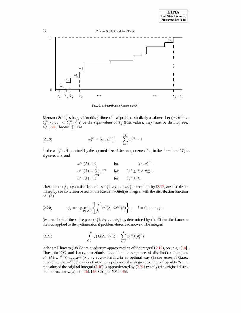
(v1 = r0/‖r0‖). For simplicity of notation we assume that all the eigenvalues of A aredistinct and increasingly ordered (an extension to the case of multiple eigenvalues will beobvious). Let ζ, ξ be such that ζ ≤ λ1 < λ2 < . . . < λn ≤ ξ. Consider the distributionfunction ω(λ) with the finite points of increase λ1, λ2, . . . , λn,

ω(λ) = 0 for λ < λ1 ,

ω(λ) =i∑l=1

ωl for λi ≤ λ < λi+1 ,

ω(λ) = 1 for λn ≤ λ ,

(2.15)

see Fig. 2.1, and the corresponding Riemann-Stieltjes integral

∫ ξ

ζ

f(λ) dω(λ) =

n∑

i=1

ωif(λi) .(2.16)

Then (2.12) can be rewritten as

ψj = arg minψ∈Mj

{∫ ξ

ζ

ψ2(λ) dω(λ)

}, j = 0, 1, 2, . . . , n .(2.17)

The j steps of the CG resp. the Lanczos method starting with ‖r0‖v1 resp. v1 determinea symmetric tridiagonal matrix (with a positive subdiagonal) Tj (2.2). Consider, analogouslyto (2.9), the eigendecomposition of Tj in the form

Tj = SjΘjSTj , STj Sj = SjS

Tj = I,(2.18)

Θj = diag(θ(j)

1 , . . . , θ(j)

j ), Sj = [s(j)

1 , . . . , s(j)

j ]. Please note that we can look at Tj also asdetermined by the CG or the Lanczos method applied to the j-dimensional problem Tjyj =e1‖r0‖ resp. Tj with initial residual e1‖r0‖ resp. starting vector e1. Clearly, we can construct



...

0

1

ω1

ω2

ω3

ω4

ωn

ζ λ1 λ2 λ3. . . . . . λn ξ

FIG. 2.1. Distribution function ω(λ)

Riemann-Stieltjes integral for this j-dimensional problem similarly as above. Let ζ ≤ θ(j)

1 <θ(j)

2 < . . . < θ(j)

j ≤ ξ be the eigenvalues of Tj (Ritz values, they must be distinct, see,e.g. [38, Chapter 7]). Let

ω(j)

i = (e1, s(j)

i )2,

j∑

i=1

ω(j)

i = 1(2.19)

be the weights determined by the squared size of the components of e1 in the direction of Tj’seigenvectors, and

ω(j)(λ) = 0 for λ < θ(j)

1 ,

ω(j)(λ) =i∑l=1

ω(j)

l for θ(j)

i ≤ λ < θ(j)

i+1,

ω(j)(λ) = 1 for θ(j)

j ≤ λ .

Then the first j polynomials from the set {1, ψ1, . . . , ψn} determined by (2.17) are also deter-mined by the condition based on the Riemann-Stieltjes integral with the distribution functionω(j)(λ)

ψl = arg minψ∈Ml

{∫ ξ

ζ

ψ2(λ) dω(j)(λ)

}, l = 0, 1, . . . , j ,(2.20)

(we can look at the subsequence {1, ψ1, . . . , ψj} as determined by the CG or the Lanczosmethod applied to the j-dimensional problem described above). The integral

∫ ξ

ζ

f(λ) dω(j)(λ) =

j∑

i=1

ω(j)

i f(θ(j)

i )(2.21)

is the well-known j-th Gauss quadrature approximation of the integral (2.16), see, e.g., [14].Thus, the CG and Lanczos methods determine the sequence of distribution functionsω(1)(λ), ω(2)(λ), . . . , ω(j)(λ), . . . approximating in an optimal way (in the sense of Gaussquadrature, i.e. ω(l)(λ) ensures that for any polynomial of degree less than of equal to 2l− 1the value of the original integral (2.16) is approximated by (2.21) exactly) the original distri-bution function ω(λ), cf. [26], [46, Chapter XV], [45].



All this is well-known. Gauss quadrature represents a classical textbook material and theconnection of CG to Gauss quadrature was pointed out in the original paper [24]. This con-nection is, however, a key to understanding both mathematical properties and finite precisionbehaviour of the CG method.

Given A and r0, (2.16) and its Gauss quadrature approximations (2.21) are for j =1, 2, . . . , n uniquely determined (remember we assumed that the eigenvalues of A are posi-tive and distinct). Conversely, the distribution function ω(j)(λ) uniquely determines the sym-metric tridiagonal matrix Tj , and, through (2.7) and (2.6), the CG approximation xj . Withf(λ) = λ−1 we have from (2.10)

‖x− x0‖2A = ‖r0‖

2n∑

i=1

ωiλi

= ‖r0‖2

∫ ξ

ζ

λ−1 dω(λ) ,(2.22)

and, using (2.3) with j = n,

‖x− x0‖2A = (r0, A

−1r0) = ‖r0‖2(e1, T

−1n e1) ≡ ‖r0‖

2 (T−1n )11 .

Consequently,

∫ ξ

ζ

λ−1 dω(λ) = (T−1n )11 .(2.23)

Repeating the same considerations using the CG method for Tj with the initial residual‖r0‖e1, or the Lanczos method for Tj with e1

∫ ξ

ζ

λ−1 dω(j)(λ) = (T−1j )11 .(2.24)

Finally, applying the j-point Gauss quadrature to (2.16) gives

∫ ξ

ζ

f(λ) dω(λ) =

∫ ξ

ζ

f(λ) dω(j)(λ) +Rj(f),(2.25)

where Rj(f) stands for the (truncation) error in the Gauss quadrature. In the next section wepresent several different ways of expressing (2.25) with f(λ) = λ−1.

3. Basic Identities. Multiplying the identity (2.25) by ‖r0‖2 gives

‖r0‖2

∫ ξ

ζ

f(λ) dω(λ) = ‖r0‖2

∫ ξ

ζ

f(λ) dω(j)(λ) + ‖r0‖2Rj(f).(3.1)

Using (2.22), (2.23) and (2.24), (3.1) can for f(λ) = λ−1 be written as

‖x− x0‖2A = ‖r0‖

2(T−1n )11 = ‖r0‖

2(T−1j )11 + ‖r0‖

2Rj(λ−1) .

In [17, pp. 253-254] it was proved that for f(λ) = λ−1 the truncation error in the Gaussquadrature is equal to

Rj(λ−1) =

‖x− xj‖2A

‖r0‖2,



which gives

‖x− x0‖2A = ‖r0‖

2(T−1j )11 + ‖x− xj‖

2A .(3.2)

Summarizing, the value of the j-th Gauss quadrature approximation to the integral (2.23) isthe complement of the error in the j-th CG iteration measured by ‖x− xj‖

2A/‖r0‖

2,

‖x− x0‖2A

‖r0‖2= j-point Gauss quadrature +

‖x− xj‖2A

‖r0‖2.(3.3)

This relation was developed in [8] in the context of moments; it was a subject of extensivework motivated by estimation of the error norms in CG in the papers [12], [15] and [17].Work in this direction continued and led to the papers [16], [28], [30], [5].

An interesting form of (3.2) was noticed by Warnick in [47]. In the papers mentionedabove the values of ‖x− x0‖

2A/‖r0‖

2 = (T−1n )11 and (T−1

j )11 were approximated from theactual Gauss quadrature calculations (or from the related recurrence relations). Using (2.7)and (2.6), the identities

‖r0‖2(T−1

j )11 = ‖r0‖ eT1 T

−1j e1‖r0‖

= ‖r0‖ vT1 Vj T

−1j e1‖r0‖ = (‖r0‖v1)

T (VjT

−1j e1‖r0‖

)

= rT0 (xj − x0)

show that (T−1j )11 is given by a simple inner product. Indeed,

‖x− x0‖2A = rT0 (xj − x0) + ‖x− xj‖

2A .(3.4)

This remarkable identity was pointed out to us by Saylor [41], [40]. Please note that deriva-tion of the identity (3.4) from the Gauss quadrature-based (3.2) uses the orthogonality relationvT1 Vj = e1. In finite precision computations this orthogonality relation does not hold. Con-sequently, (3.4) does not hold in finite precision arithmetic. We will return to this point inSection 6.

A mathematically equivalent identity can be derived by simple algebraic manipulationswithout using Gauss quadrature,

(x− x0)TA(x− x0) = (x− xj + xj − x0)

TA(x − x0)

= (x− xj)TA(x − x0) + (xj − x0)

TA(x− x0)

= (x− xj)TA(x − xj + xj − x0) + (xj − x0)

T r0

= ‖x− xj‖2A + (x− xj)

TA(xj − x0) + rT0 (xj − x0)

= ‖x− xj‖2A + rTj (xj − x0) + rT0 (xj − x0),

hence

‖x− x0‖2A = rTj (xj − x0) + rT0 (xj − x0) + ‖x− xj‖

2A.(3.5)

The right-hand side of (3.5) contains, in comparison with (3.4), the additional term rTj (xj −x0). This term is in exact arithmetic equal to zero, but it has an important correction effect infinite precision computations (see Section 6).

Relations (3.2), (3.4) and (3.5) represent various mathematically equivalent forms of(3.1). While in (3.2) the j-point Gauss quadrature is evaluated as (T−1

j )11, in (3.4) and (3.5)this quantity is computed using inner products of the vectors that are at our disposal during



the iteration process. But, as mentioned in Introduction, there is much simpler identity (1.5)mathematically equivalent to (3.1). It is very surprising that, though (1.5) is present in theHestenes and Stiefel paper [24, Theorem 6.1, relation (6:2), p. 416], this identity has (at leastto our knowledge) never been related to Gauss quadrature. Its derivation is very simple. Using(1.3)

‖x− xi‖2A − ‖x− xi+1‖

2A = ‖x− xi+1 + xi+1 − xi‖

2A − ‖x− xi+1‖

2A

= ‖xi+1 − xi‖2A + 2(x− xi+1)

TA(xi+1 − xi)

= γ2i p

Ti Api + 2rTi+1(xi+1 − xi)

= γi‖ri‖2 .(3.6)

Consequently, for 0 ≤ l < j ≤ n,

‖x− xl‖2A − ‖x− xj‖

2A =

j−1∑

i=l

(‖x− xi‖

2A − ‖x− xi+1‖

2A

)=

j−1∑

i=l

γi‖ri‖2,(3.7)

and (3.1) can be written in the form

‖x− x0‖2A =

j−1∑

i=0

γi‖ri‖2 + ‖x− xj‖

2A.(3.8)

The numbers γi‖ri‖2 are trivially computable; both γi and ‖ri‖2 are available at every iter-

ation step. Please note that in the derivation of (3.7) we used the local orthogonality amongthe consecutive residuals and direction vectors only. We avoided using mutual orthogonalityamong the vectors with generally different indices. This fact will be very important in therounding error analysis of the finite precision counterparts of (3.7) in Sections 7–10.

4. Estimating the A-norm of the error. Using ‖x − x0‖2A = ‖r0‖

2(T−1n )11, (3.2) is

written in the form

‖x− xj‖2A = ‖r0‖

2[(T−1n )11 − (T−1

j )11].

As suggested in [17, pp. 28–29], the unknown value (T−1n )11 can be replaced, at a price of

m− j extra steps, by a computable value (T−1m )11 for somem > j. The paper [17], however,

did not properly use this idea and did not give a proper formula for computing the difference(T−1m )11 − (T−1

j )11 without cancellation, which limited the applicability of the proposedresult. Golub and Meurant cleverly resolved this trouble in [16] and proposed an algorithmfor estimating the A-norm of the error in the CG method called CGQL. This section willbriefly summarize several important estimates.

Consider, in general, (3.1) for j and j + d, where d is some positive integer. The idea issimply to eliminate the unknown term

∫ ξζ f(λ) dω(λ) by subtracting the identities for j and

j + d which results in

‖r0‖2Rj(f) = ‖r0‖

2

( ∫ ξ

ζ

f(λ) dω(j+d)(λ) −

∫ ξ

ζ

f(λ) dω(j)(λ)

)+‖r0‖

2Rj+d(f).

In particular, using (3.2), (3.4), (3.5), and (3.8) we obtain the mathematically equivalent iden-tities

‖x− xj‖2A = ‖r0‖

2 [(T−1j+d)11 − (T−1

j )11] + ‖x− xj+d‖2A ,(4.1)

‖x− xj‖2A = rT0 (xj+d − xj) + ‖x− xj+d‖

2A ,(4.2)

‖x− xj‖2A = rT0 (xj+d − xj) − rTj (xj − x0) + rTj+d(xj+d − x0)(4.3)

+ ‖x− xj+d‖2A ,



and

‖x− xj‖2A =

j+d−1∑

i=j

γi‖ri‖2 + ‖x− xj+d‖

2A .(4.4)

Now recall that theA-norm of the error is in the CG method strictly decreasing. If d is chosensuch that

‖x− xj‖2A � ‖x− xj+d‖

2A ,(4.5)

then neglecting ‖x − xj+d‖2A on the right-hand sides of (4.1), (4.2), (4.3) and (4.4) gives

lower bounds (all mathematically equal) for the squared A-norm of the error in the j-th step.Under the assumption (4.5) these bounds are reasonably tight (their inaccuracy is given by‖x− xj+d‖

2A). We denote them

ηj,d = ‖r0‖2 [(T−1

j+d)11 − (T−1j )11],(4.6)

where the difference (T−1j+d)11 − (T−1

j )11 is computed by the algorithm CGQL from [16],

µj,d = rT0 (xj+d − xj),(4.7)

which refers to the original bound due to Warnick,

ϑj,d = rT0 (xj+d − xj) − rTj (xj − x0) + rTj+d(xj+d − x0),(4.8)

which is the previous bound modified by the correction terms and

νj,d =

j+d−1∑

i=j

γi‖ri‖2.(4.9)

Clearly, the last bound, which is a direct consequence of [24, Theorem 6:1], see (1.5), is muchsimpler than the others.

Mathematically (in exact arithmetic)

ηj,d = µj,d = ϑj,d = νj,d .(4.10)

In finite precision computations (4.10) does not hold in general, and the different boundsmay give substantially different results. Does any of the identities (4.1)–(4.4) have any rele-vance for the quantities computed in finite precision arithmetic? The work described in thissubsection and the papers published on this subject would be of little practical use withoutanswering this question.

5. Delay of convergence. For more than 20 years the effects of rounding errors to theLanczos and CG methods seemed devastating. Orthogonality among the computed vectorsv1, v2, . . . was usually lost very quickly, with a subsequent loss of linear independence. Con-sequently, the finite termination property was lost. Still, despite a total loss of orthogonalityamong the vectors in the Lanczos sequence v1, v2, . . . , and despite a possible regular appear-ance of Lanczos vectors which were linearly dependent on the vectors computed in precedingiterations, the Lanczos and the CG methods produced reasonable results.

A fundamental work which brought light into this darkness was done by Paige. Heproved that loss of orthogonality among the computed Lanczos vectors v1, v2, . . . was pos-sible only in the directions of the converged Ritz vectors z(j)

l ≡ Vjs(j)

l . For more details



see [33], [34], [35], [36], the review paper [44, Section 3.1] and the works quoted there (inparticular [38], [39], [32] and [45]). Little was known about rounding errors in the Krylovsubspace methods before the Ph.D. thesis of Paige [33], and almost all results (with the ex-ception of works on ultimate attainable accuracy) published on the subject after this thesisand the papers [34], [35], [36] were based on them.

Another step, which can compete in originality with that of Paige, was made by Green-baum in [19]. If CG is used to solve a linear symmetric positive definite system Ax = b on acomputer with machine precision ε, then [19] shows that theA-norms of the errors ‖x−xl‖A,l = 1, 2, . . . , j are very close to the A-norms of the errors ‖x − xl‖A, l = 1, 2, . . . , jdetermined by the exact CG applied to some particular symmetric positive definite systemA(j)x(j) = b(j) (see [19, Theorem 3, pp. 26-27]). This system and the initial approxima-tion x0(j) depend on the iteration step j. The matrix A(j) is larger than the matrix A. Itseigenvalues must lie in tiny intervals about the eigenvalues of A, and there must be at leastone eigenvalue of A(j) close to each eigenvalue of A (the last result was proved in [43]).Moreover, for each eigenvalue λi of A, i = 1, . . . , n (similarly to Section 2 we assume,with no loss of generality, that the eigenvalues of A are distinct), the weight ωi = (v1, ui)

2

closely approximates the sum of weights corresponding to the eigenvalues of A(j) clusteredaround λi (see [19, relation (8.21) on p. 60]).

The quantitative formulations of the relationships betweenA, b, x0 andA(j), b(j), x0(j)contains some terms related in various complicated ways to machine precision ε (see [19],[43] and [17, Theorems 5.1–5.3 and the related discussion on pp. 257–260]). The actual sizeof the terms given in the quoted papers documents much more difficulties of handling accu-rately peculiar technical problems of rounding error analysis than it says about the accuracy ofthe described relationships. The fundamental concept to which the (very often weak) round-ing error bounds lead should be read: the first j steps of a finite precision CG computationforAx = b can be viewed as the first j steps of the exact CG computation for some particularA(j)x(j) = b(j). This relationship was developed and proved theoretically. Numerical ex-periments show that its tightness is much better than the technically complicated theoreticalcalculations in [19] would suggest. We will not continue with describing the results of thesubsequent work [22]. We do not need it here. Moreover, a rigorous theoretical descriptionof the model from [22] in the language of Riemann-Stieltjes integral and Gauss quadraturestill needs some clarification. We hope to return to that subject elsewhere.

As a consequence of the loss of orthogonality caused by rounding errors, convergenceof the CG method is delayed. In order to illustrate this important point numerically, weplot in Fig. 5.1 results of the CG method (1.3) for the matrix A = QΛQT , where Q is theorthogonal matrix obtained from the Matlab QR-decomposition of the randomly generatedmatrix (computed by the Matlab command randn(n)), and Λ = diag(λ1, . . . , λn) is adiagonal matrix with the eigenvalues

λi = λ1 +i− 1

n− 1(λn − λ1) ρ

n−i, i = 2, . . . , n− 1,(5.1)

see [43]. We have used n = 48, λ1 = 0.1, λn = 1000, ρ = 0.9, x = (1, . . . , 1)T , b = Ax,and x0 = (0, . . . , 0)T . We have simulated the exact arithmetic values by double reorthogo-nalization of the residual vectors (see [22]). The quantities obtained from the CG implemen-tation with the double reorthogonalized residuals will be denoted by (E). Fig. 5.1 shows thatwhen the double reorthogonalization is applied, the correspondingA-norm of the error (dash-dotted line) can be very different from theA-norm of the error of the ordinary finite precision(FP) CG implementation (solid line). Without reorthogonalization, the orthogonality amongthe (FP) Lanczos vectors, measured by the Frobenius norm ‖I − V T

j Vj‖F (dotted line), is



0 20 40 60 80 100 120

10−16

10−14

10−12

10−10

10−8

10−6

10−4

10−2

100

(E) || x−xj ||

A

(FP) || x−xj ||

A

(E) || I−VTjV

j ||

F(FP) || I−VT

jV

j ||

F

FIG. 5.1. The A-norm of the error for the CG implementation with the double reorthogonalized residuals (E)(dashed-dotted line) is compared to the A-norm of the error of the ordinary finite precision CG implementation (FP)(solid line). The corresponding loss of orthogonality among the normalized residuals is plotted by the dots resp. thedotted line.

lost after a few iterations. With double reorthogonalization the orthogonality is kept closeto machine precision (dots). Experiments were performed using Matlab 5.1 on a personalcomputer with machine precision ε ∼ 10−16.

We see that the delay of convergence due to loss of orthogonality can be very substan-tial. Consider now application of the estimates (4.6)–(4.9) to finite precision computations.In derivation of all these estimates we assumed exact arithmetic. Consequently, in thesederivations we did not count for any loss of orthogonality and delay of convergence. Forthe example presented above, the bounds can therefore be expected to give good results forthe double reorthogonalized CG (dash-dotted convergence curve). Should they give anythingreasonable also for the ordinary (FP) CG implementation (solid convergence curve)? If yes,then why? The following section explains that this question is of fundamental importance.

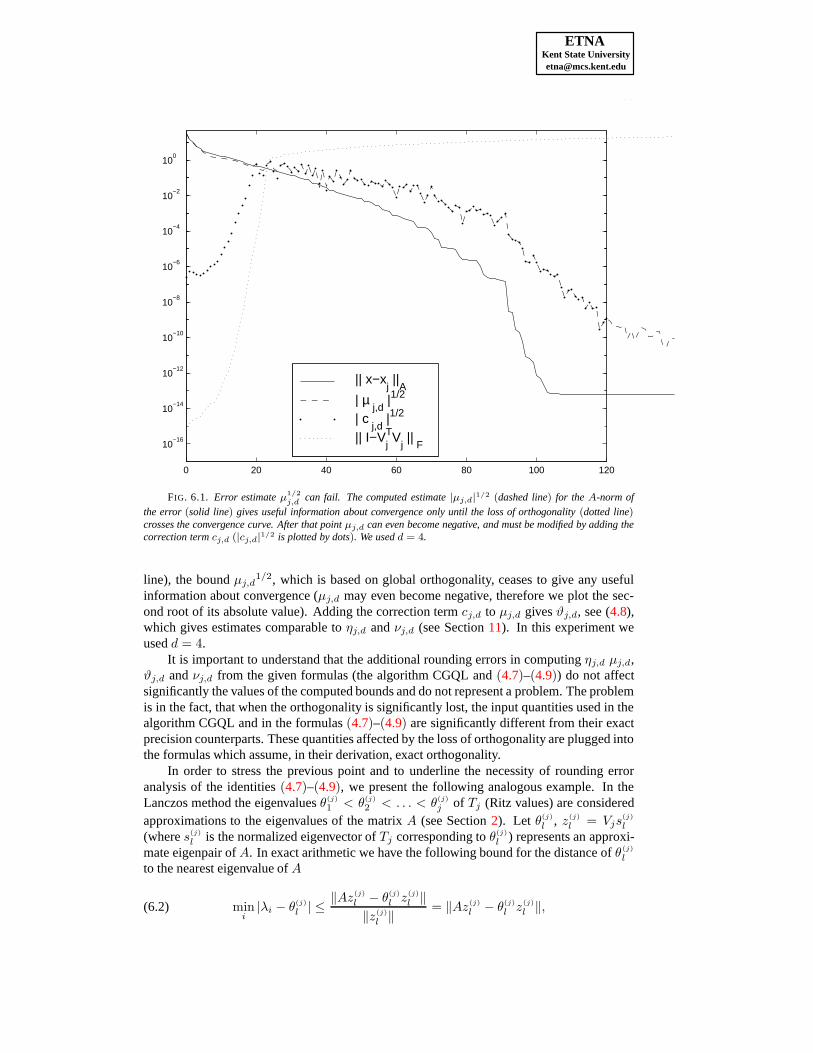
6. Examples. Indeed, without a proper rounding error analysis of the identities (4.1)–(4.4) there is no justification that the estimates derived assuming exact arithmetic will workin finite precision arithmetic. For example, when the significant loss of orthogonality occurs,the bound µj,d given by (4.7) does not work!

This fact is demonstrated in Fig. 6.1 which presents experimental results for the problemdescribed in the previous section (see Fig. 5.1). It plots the computed estimate |µj,d|

1/2

(dashed line) and demonstrates the importance of the correction term

cj,d = −rTj (xj − x0) + rTj+d(xj+d − x0),(6.1)

( |cj,d|1/2 is plotted by dots). Fig. 6.1 shows clearly that when the global orthogonality (mea-sured by ‖I − V Tj Vj‖F and plotted by a dotted line) grows greater than ‖x − xj‖A (solid



0 20 40 60 80 100 120

10−16

10−14

10−12

10−10

10−8

10−6

10−4

10−2

100

|| x−xj ||

A

| µ j,d

|1/2 | c

j,d |1/2

|| I−VTjV

j ||

F

FIG. 6.1. Error estimate µ1/2

j,dcan fail. The computed estimate |µj,d|

1/2 (dashed line) for the A-norm of

the error (solid line) gives useful information about convergence only until the loss of orthogonality (dotted line)crosses the convergence curve. After that point µj,d can even become negative, and must be modified by adding thecorrection term cj,d (|cj,d|

1/2 is plotted by dots). We used d = 4.

line), the bound µj,d1/2, which is based on global orthogonality, ceases to give any usefulinformation about convergence (µj,d may even become negative, therefore we plot the sec-ond root of its absolute value). Adding the correction term cj,d to µj,d gives ϑj,d, see (4.8),which gives estimates comparable to ηj,d and νj,d (see Section 11). In this experiment weused d = 4.

It is important to understand that the additional rounding errors in computing ηj,d µj,d,ϑj,d and νj,d from the given formulas (the algorithm CGQL and (4.7)–(4.9)) do not affectsignificantly the values of the computed bounds and do not represent a problem. The problemis in the fact, that when the orthogonality is significantly lost, the input quantities used in thealgorithm CGQL and in the formulas (4.7)–(4.9) are significantly different from their exactprecision counterparts. These quantities affected by the loss of orthogonality are plugged intothe formulas which assume, in their derivation, exact orthogonality.

In order to stress the previous point and to underline the necessity of rounding erroranalysis of the identities (4.7)–(4.9), we present the following analogous example. In theLanczos method the eigenvalues θ(j)

1 < θ(j)

2 < . . . < θ(j)

j of Tj (Ritz values) are consideredapproximations to the eigenvalues of the matrix A (see Section 2). Let θ(j)

l , z(j)

l = Vjs(j)

l

(where s(j)

l is the normalized eigenvector of Tj corresponding to θ(j)

l ) represents an approxi-mate eigenpair of A. In exact arithmetic we have the following bound for the distance of θ(j)

l

to the nearest eigenvalue of A

mini

|λi − θ(j)

l | ≤‖Az(j)

l − θ(j)

l z(j)

l ‖

‖z(j)

l ‖= ‖Az(j)

l − θ(j)

l z(j)

l ‖,(6.2)



where ‖z(j)

l ‖ = 1 due to the orthonormality of the Lanczos vectors v1, . . . , vj . Using (2.3),‖Az(j)

l − θ(j)

l z(j)

l ‖ = βj+1(ej , s(j)

l ), which gives

mini

|λi − θ(j)

l | ≤ βj+1(ej , s(j)

l ) ≡ δlj ,(6.3)

see, e.g., [38], [36]. Consequently, in exact arithmetic, if δlj is small, then θ(j)

l must be closeto some λi. In finite precision arithmetic loss of orthogonality has, among the others, a veryunpleasant effect: we cannot guarantee, in general, that z(j)

l , which is a linear combination ofv1, . . . , vj has a nonvanishing norm. We can still compute δlj from βj+1 and Tj ; the effect ofrounding errors in this additional computation is negligible. We can therefore say, similarlyto the analogous statements published about computation of the convergence estimates in theCG method, that δlj is in the presence of rounding errors computed “accurately”. Does δljcomputed in finite precision arithmetic tell anything about convergence of θ(j)

l to some λi?Yes, it does! But this affirmative answer is based neither on the exact precision formulas(6.2) and (6.3), nor on the fact that δlj is computed “accurately”. It is based on an ingeniousanalysis due to Paige, who have shown that the orthogonality can be lost in the directions ofthe well approximated eigenvectors only. For the complicated details of this difficult resultwe refer to [33], [37] and to the summary given in [44, Theorem 2]. We see that even in finiteprecision computations small δlj guarantees that θ(j)

l approximates some λi to high accuracy.It is very clear, however, that this conclusion is the result of the rounding error analysis ofthe Lanczos method given by Paige, and no similar statement could be made without thisanalysis.

In the following three sections we present rounding error analysis of the bound νj,d givenby (4.4) and (4.9). We concentrate on νj,d because it is the simplest of all the others. If νj,dis proved numerically stable, then there is a small reason for using the other bounds ηj,d orϑj,d in practical computations.

7. Finite precision CG computations. In the analysis we assume the standard modelof floating point arithmetic with machine precision ε, see, e.g. [25, (2.4)],

fl[a ◦ b] = (a ◦ b)(1 + δ), |δ| ≤ ε,(7.1)

where a and b stands for floating-point numbers and the symbol ◦ stands for the operationsaddition, subtraction, multiplication and division. We assume that this model holds also forthe square root operation. Under this model, we have for operations involving vectors v, w, ascalar α and the matrix A the following standard results [18], see also [20], [35]

‖α v − fl[α v]‖ ≤ ε ‖α v‖,(7.2)

‖v + w − fl[v + w]‖ ≤ ε (‖v‖ + ‖w‖),(7.3)

|(v, w) − fl[(v, w)]| ≤ ε n (1 +O(ε)) ‖v‖ ‖w‖,(7.4)

‖Av − fl[Av]‖ ≤ ε c ‖A‖‖v‖.(7.5)

When A is a matrix with at most h nonzeros in any row and if the matrix-vector product iscomputed in the standard way, c = hn1/2. In the following analysis we count only for theterms linear in the machine precision epsilon ε and express the higher order terms as O(ε2).By O(const) where const is different from ε2 we denote const multiplied by a boundedpositive term of an insignificant size which is independent of the const and of any othervariables present in the bounds.

Numerically, the CG iterates satisfy

xj+1 = xj + γjpj + εzxj ,(7.6)



rj+1 = rj − γjApj + εzrj ,(7.7)

pj+1 = rj+1 + δj+1pj + εzpj ,(7.8)

where εzxj , εzrj and εzpj account for the local roundoff (r0 = b − Ax0 − εf0, ε‖f0‖ ≤

ε{‖b‖+ ‖Ax0‖+ c‖A‖‖x0‖}+O(ε2)). The local roundoff can be bounded according to thestandard results (7.2)–(7.5) in the following way

ε ‖zxj ‖ ≤ ε {‖xj‖ + 2 ‖γjpj‖}+O(ε2) ≤ ε {3‖xj‖ + 2‖xj+1‖}+O(ε2),(7.9)

ε ‖zrj‖ ≤ ε {‖rj‖ + 2 ‖γjApj‖ + c ‖A‖‖γjpj‖} +O(ε2),(7.10)

ε ‖zpj ‖ ≤ ε {‖rj+1‖ + 2 ‖δj+1pj‖}+O(ε2) ≤ ε {3‖rj+1‖ + 2‖pj+1‖} +O(ε2).(7.11)

Similarly, the computed coefficients γj and δj satisfy

γj =‖rj‖

2

pTj Apj+ εζγj , δj =

‖rj‖2

‖rj−1‖2+ εζδj .(7.12)

Assuming nε� 1, the local roundoff εζδj is bounded, according to (7.1) and (7.4), by

ε|ζδj | ≤ ε‖rj‖

2

‖rj−1‖2O(n) +O(ε2).(7.13)

Using (7.2)–(7.5) and ‖A‖‖pj‖2/(pj , Apj) ≤ κ(A),

fl[(pj , Apj)] = (pj , Apj) + ε ‖Apj‖‖pj‖O(n) + ε ‖A‖‖pj‖2O(c) +O(ε2)

= (pj , Apj)(1 + ε κ(A)O(n + c)

)+O(ε2).

Assuming ε(n+ c)κ(A) � 1, the local roundoff εζγj is bounded by

ε|ζγj | ≤ ε κ(A)‖rj‖

2

(pj , Apj)O(n+ c) +O(ε2).(7.14)

It is well-known that in finite precision arithmetic the true residual b−Axj differs fromthe recursively updated residual vector rj ,

rj = b−Axj − εfj .(7.15)

This topic was studied in [42] and [20]. The results can be written in the following form

‖εfj‖ ≤ ε ‖A‖ (‖x‖+ max0≤i≤j

‖xi‖)O(jc),(7.16)

‖rj‖ = ‖b−Axj‖ (1 + εFj),(7.17)

where εFj is bounded by

|εFj | =|‖rj‖ − ‖b−Axj‖|

‖b−Axj‖≤

‖rj − (b−Axj)‖

‖b−Axj‖=

ε‖fj‖

‖b−Axj‖.(7.18)

Rounding errors affect results of CG computations in two main ways: they delay con-vergence (see Section 5) and limit the ultimate attainable accuracy. Here we are primarilyinterested in estimating the convergence rate. We therefore assume that the final accuracylevel has not been reached yet and εfj is, in comparison to the size of the true and itera-tive residuals, small. In the subsequent text we will relate the numerical inaccuracies to the



A-norm of the error ‖x − xj‖A. The following inequalities derived from (7.18) will proveuseful,

λ1/21 ‖x− xj‖A (1 + ε Fj) ≤ ‖rj‖ ≤ λ1/2

n ‖x− xj‖A (1 + ε Fj).(7.19)

The monotonicity of the A-norm and of the Euclidean norm of the error is in CG preserved(with small additional inaccuracy) also in finite precision computations (see [19], [22]). Usingthis fact we get for j ≥ i

ε‖rj‖

‖ri‖≤ ε

λ1/2n

λ1/21

·‖x− xj‖A‖x− xi‖A

·(1 + ε Fj)

(1 + ε Fi)≤ ε κ(A)1/2 +O(ε2).(7.20)

This bound will be used later.

8. Finite precision analysis – basic identity. The bounds (4.6)–(4.9) are mathemati-cally equivalent. We will concentrate on the simplest one given by νj,d (4.9) and prove that itgives (up to a small term) correct estimates also in finite precision computations. In particular,we prove that the ideal (exact precision) identity (4.4) changes numerically to

‖x− xj‖2A = νj,d + ‖x− xj+d‖

2A + νj,d,(8.1)

where νj,d is as small as it can be (the analysis here will lead to much stronger results thanthe analysis of the finite precision counterpart of (4.1) given in [17]). Please note that thedifference between (4.4) and (8.1) is not trivial. The ideal and numerical counterparts of eachindividual term in these identities may be orders of magnitude different! Due to the facts thatrounding errors in computing νj,d numerically from the quantities γi, ri are negligible andthat νj,d will be related to ε ‖x− xj‖A, (8.1) will justify the estimate νj,d in finite precisioncomputations.

From the identity for the numerically computed approximate solution

‖x− xj‖2A = ‖x− xj+1 + xj+1 − xj‖

2A

= ‖x− xj+1‖2A + 2 (x− xj+1)

TA(xj+1 − xj) + ‖xj+1 − xj‖2A,

we obtain easily

‖x− xj‖2A − ‖x− xj+1‖

2A = ‖xj+1 − xj‖

2A + 2 (x− xj+1)

TA(xj+1 − xj).(8.2)

Please note that (8.2) represents an identity for the computed quantities. In order to get thedesired form leading to (8.1), we will develop the right hand side of (8.2). In this derivationwe will rely on local properties of the finite precision CG recurrences (7.6)–(7.8) and (7.12).

Using (7.6), the first term on the right hand side of (8.2) can be written as

‖xj+1 − xj‖2A = (γjpj + ε zxj )

TA(γjpj + ε zxj )

= γ2j p

Tj Apj + 2ε γjp

Tj Az

xj +O(ε2)

= γ2j p

Tj Apj + 2ε (xj+1 − xj)

TAzxj +O(ε2).(8.3)

Similarly, the second term on the right hand side of (8.2) transforms, using (7.15), to the form

2 (x− xj+1)TA(xj+1 − xj) = 2 (rj+1 + ε fj+1)

T (xj+1 − xj)

= 2 rTj+1(xj+1 − xj) + 2ε fTj+1(xj+1 − xj).(8.4)



Combining (8.2), (8.3) and (8.4),

‖x− xj‖2A − ‖x− xj+1‖

2A = γ2

j pTj Apj + 2 rTj+1(xj+1 − xj)

+ 2ε (fj+1 +Azxj )T (xj+1 − xj) +O(ε2).(8.5)

Substituting for γj from (7.12), the first term in (8.5) can be written as

γ2j p

Tj Apj = γj‖rj‖

2 + ε γj pTj Apj ζ

γj = γj‖rj‖

2 + ε γj‖rj‖2

{ζγjpTj Apj

‖rj‖2

}.

Consequently, the difference between the squared A-norms of the error in the consecutivesteps can be written in the form convenient for the further analysis

‖x− xj‖2A − ‖x− xj+1‖

2A = γj‖rj‖

2 + ε γj‖rj‖2

{ζγjpTj Apj

‖rj‖2

}(8.6)

+ 2 rTj+1(xj+1 − xj)

+ 2ε (fj+1 +Azxj )T (xj+1 − xj) +O(ε2).

The goal of the following analysis is to show that until ‖x − xj‖A reaches its ultimateattainable accuracy level, the terms on the right hand side of (8.6) are, except for γj‖rj‖2,insignificant. Bounding the second term will not represent a problem. The norm of the dif-ference xj+1 − xj = (x − xj) − (x − xj+1) is bounded by 2‖x − xj‖A/λ

1/2

1 . Thereforethe size of the fourth term is proportional to ε ‖x − xj‖A. The third term is related to theline-search principle. Ideally (in exact arithmetic), the (j + 1)-th residual is orthogonal tothe difference between the (j + 1)-th and j-th approximation (which is a multiple of the j-thdirection vector). This is equivalent to the line-search: ideally the (j + 1)-th CG approxima-tion minimizes the A-norm of the error along the line determined by the j-th approximationand the j-th direction vector. Here the term rTj+1(xj+1 − xj), with rj+1, xj and xj+1 com-puted numerically, examines how closely the line-search holds in finite precision arithmetic.In fact, bounding the local orthogonality rTj+1(xj+1 − xj) represents the technically mostdifficult part of the remaining analysis.

9. Local orthogonality in the Hestenes and Stiefel implementation. Since the classi-cal work of Paige it is well-known that in the three-term Lanczos recurrence local orthogo-nality is preserved close to the machine epsilon (see [35]). We will derive an analogy of thisfor the CG algorithm, and state it as an independent result.

The local orthogonality term rTj+1(xj+1 − xj) can be written in the form

rTj+1(xj+1 − xj) = rTj+1(γjpj + ε zxj ) = γjrTj+1pj + ε rTj+1z

xj .(9.1)

Using the bound ‖rj+1‖ ≤ λ1/2n ‖x − xj+1‖A(1 + ε Fj+1) ≤ λ

1/2n ‖x − xj‖A(1 + ε Fj+1),

see (7.19), the size of the second term in (9.1) is proportional to ε ‖x− xj‖A. The main stepconsist of showing that the term rTj+1pj is sufficiently small. Multiplying the recurrence (7.7)for rj+1 by the column vector pTj gives (using (7.8) and (7.12))

pTj rj+1 = pTj rj − γjpTj Apj + ε pTj z

rj

= (rj + δjpj−1 + ε zpj−1)T rj −

(‖rj‖

2

pTj Apj+ ε ζγj

)pTj Apj + ε pTj z

rj

= δj pTj−1rj + ε {rTj z

pj−1 − ζγj p

Tj Apj + pTj z

rj }.(9.2)



Denoting

Mj ≡ rTj zpj−1 − ζγj p

Tj Apj + pTj z

rj ,(9.3)

the identity (9.2) is

pTj rj+1 = δj pTj−1rj + εMj .(9.4)

Recursive application of (9.4) for pTj−1rj , . . . , pT1 r2 with pT0 r1 = ‖r0‖

2 − γ0 pT0 Ap0 +

ε pT0 zr0 = ε {−ζγ0 r

T0 Ar0 + pT0 z

r0} ≡ εM0, gives

pTj rj+1 = εMj + ε

j∑

i=1

( j∏

k=i

δk

)Mi−1.(9.5)

Since

ε

j∏

k=i

δk = ε

j∏

k=i

‖rk‖2

‖rk−1‖2+O(ε2) = ε

‖rj‖2

‖ri−1‖2+O(ε2),

we can express (9.5) as

pTj rj+1 = ε ‖rj‖2

j∑

i=0

Mi

‖ri‖2+O(ε2).(9.6)

Using (9.3),

|Mi|

‖ri‖2≤

‖zpi−1‖

‖ri‖+ |ζγi |

pTi Api‖ri‖2

+‖pi‖‖z

ri ‖

‖ri‖2.(9.7)

¿From (7.11) it follows

ε‖zpi−1‖

‖ri‖≤ ε

{3 + 2

‖pi‖

‖ri‖

}+O(ε2).(9.8)

Using (7.14),

ε |ζγi |pTi Api‖ri‖2

≤ ε κ(A)O(n+ c) +O(ε2).(9.9)

The last part of (9.7) is bounded using (7.10) and (7.12)

ε‖pi‖‖z

ri ‖

‖ri‖2≤ ε

{‖pi‖‖ri‖

‖ri‖2+ 2 γi

‖pi‖‖Api‖

‖ri‖2+ c γi

‖pi‖‖A‖‖pi‖

‖ri‖2

}+O(ε2)

= ε

{‖pi‖

‖ri‖+ 2

‖pi‖‖Api‖

pTi Api+ c

‖A‖‖pi‖2

pTi Api

}+O(ε2)

≤ ε

{‖pi‖

‖ri‖+ (2 + c)κ(A)

}+O(ε2),(9.10)

where

ε‖pi‖

‖ri‖≤ ε

‖ri‖ + δi‖pi−1‖

‖ri‖+O(ε2) ≤ ε

{1 +

‖ri‖

‖ri−1‖

‖pi−1‖

‖ri−1‖

}+O(ε2).(9.11)



Recursive application of (9.11) for ‖pi−1‖/‖ri−1‖, ‖pi−2‖/‖ri−2‖, . . ., ‖p1‖/‖r1‖ with‖p0‖/‖r0‖ = 1 gives

ε‖pi‖

‖ri‖≤ ε

{1 +

‖ri‖

‖ri−1‖+

‖ri‖

‖ri−2‖+ . . .+

‖ri‖

‖r0‖

}+O(ε2).(9.12)

The size of ε ‖ri‖/‖rk‖, i ≥ k is, according to (7.20), less or equal than ε κ(A)1/2 +O(ε2).Consequently,

ε‖pi‖

‖ri‖≤ ε {1 + i κ(A)1/2} +O(ε2).(9.13)

Summarizing (9.8), (9.9), (9.10) and (9.13), the ratio ε |Mi|/‖ri‖2 is bounded as

ε|Mi|

‖ri‖2≤ ε κ(A)O(8 + 2c+ n+ 3i) +O(ε2).(9.14)

Combining this result with (9.6) proves the following theorem.

THEOREM 9.1. Using the previous notation, let ε (n + c)κ(A) � 1. Then the lo-cal orthogonality between the direction vectors and the iteratively computed residuals is inthe finite precision implementation of the conjugate gradient method (7.6)–(7.8) and (7.12)bounded by

|pTj rj+1| ≤ ε ‖rj‖2κ(A)O((j + 1)(8 + 2c+ n+ 3j)) +O(ε2).(9.15)

10. Final precision analysis – conclusions. We now return to (8.6) and finalize ourdiscussion. Using (9.1) and (9.6),

‖x− xj‖2A − ‖x− xj+1‖

2A = γj‖rj‖

2(10.1)

+ ε γj‖rj‖2

{ζγjpTj Apj

‖rj‖2+ 2

j∑

i=0

Mi

‖ri‖2

}

+ 2ε {(fj+1 +Azxj )T (xj+1 − xj) + rTj+1z

xj }

+O(ε2).

The term

E(1)

j ≡ ε

{ζγjpTj Apj

‖rj‖2+ 2

j∑

i=0

Mi

‖ri‖2

}

is bounded using (7.14) and (9.14),

|E(1)

j | ≤ ε κ(A)O(n+ c+ 2(j + 1)(8 + 2c+ n+ 3j)) +O(ε2).(10.2)

We write the remaining term on the right hand side of (10.1) proportional to ε as

2ε {(fj+1 +Azxj )T (xj+1 − xj) + rTj+1zxj } ≡ ‖x− xj‖AE

(2)

j ,(10.3)

where

|E(2)

j | = 2ε

∣∣∣∣(fj+1 +Azxj )T

(xj+1 − x+ x− xj

‖x− xj‖A

)+

rTj+1

‖x− xj‖Azxj

∣∣∣∣

≤ 2ε {2 (‖fj+1‖λ−1/21 + ‖A‖1/2‖zxj ‖) + ‖A‖1/2‖zxj ‖}.(10.4)



With (7.16) and (7.9),

|E(2)

j | ≤ 4ε‖A‖1/2κ(A)1/2(‖x‖ + max0≤i≤j+1

‖xi‖)O(jc)

+ 5‖A‖1/2ε(3‖xj‖+ 2‖xj+1‖) +O(ε2)

≤ ε‖A‖1/2κ(A)1/2(‖x‖ + max0≤i≤j+1

‖xi‖)O(4jc+ 25) +O(ε2).(10.5)

Finally, using the fact that the monotonicity of the A-norm and the Euclidean norm of theerror is preserved also in finite precision CG computations (with small additional inaccuracy,see [19], [22]), we obtain the finite precision analogy of (4.4), which is formulated as atheorem.

THEOREM 10.1. With the notation defined above, let ε (n+ c)κ(A) � 1. Then the CGapproximate solutions computed in finite precision arithmetic satisfy

‖x− xj‖2A − ‖x− xj+d‖

2A = νj,d + νj,d E

(1)

j,d + ‖x− xj‖AE(2)

j,d +O(ε2),(10.6)

where

νj,d =

j+d−1∑

i=j

γi‖ri‖2(10.7)

and the terms due to rounding errors are bounded by

|E(1)

j,d| ≤ O(d) maxj≤i≤j+d−1

|E(1)

i |,(10.8)

|E(1)

i | ≤ ε κ(A)O(t(1)(n)) +O(ε2),

|E(2)

j,d| ≤ O(d) maxj≤i≤j+d−1

|E(2)

i |,(10.9)

|E(2)

i | ≤ ε ‖A‖1/2κ(A)1/2(‖x‖ + max0≤i≤j+1

‖xi‖)O(t(2)(n)) +O(ε2).

O(t(1)(n)) and O(t(2)(n)) represent terms bounded by a small degree polynomial in n inde-pendent of any other variables.

Please note that the value νj,d is in Theorem 10.1 computed exactly using (10.7). Errors incomputing νj,d numerically (i.e. in computing fl(

∑j+d−1i=j γi‖ri‖

2)) are negligible in com-parison to νj,d multiplied by the bound for the term |E(1)

i | and need not be considered here.Theorem 10.1 therefore says that for the numerically computed approximate solutions

‖x− xj‖2A − ‖x− xj+d‖

2A = fl(νj,d) + νj,d,(10.10)

where the term νj,d “perturbes” the ideal identity (4.4) in the finite precision case. Here νj,ddenotes quantity insignificantly different from νj,d in (8.1). Consequently, the numericallycomputed value νj,d can be trusted until it reaches the level of νj,d. Based on the assumptionε(n+c)κ(A) � 1 and (10.8) we consider |E(1)

i | � 1. Then, assuming (4.5), the numericallycomputed value νj,d gives a good estimate for the A-norm of the error ‖x− xj‖

2A until

‖x− xj‖A |E(2)

j,d| � ‖x− xj‖2A,

which is equivalent to

‖x− xj‖A � |E(2)

j,d|.(10.11)



0 20 40 60 80 100 120

10−16

10−14

10−12

10−10

10−8

10−6

10−4

10−2

100

|| x−xj ||

A

η j,d

1/2

ϑ j,d

1/2

ν j,d

1/2 || ε f

j ||

|| I−VTjV

j ||

F

FIG. 11.1. Error estimates η1/2

j,d(dots), ϑ

1/2

j,d(dashed-line) and ν

1/2

j,d(dash-doted line). They essentially

coincide until ‖x − xj‖A (solid line) reaches its ultimate attainable accuracy. The loss of orthogonality is plottedby the dotted line. We used d = 4.

The value E(2)

j,d represents various terms. Its upper bound is, apart from κ(A)1/2, whichcomes into play as an effect of the worst-case rounding error analysis, linearly dependenton an upper bound for ‖x − x0‖A. The value of E(2)

j,d is (as similar terms or constants inany other rounding error analysis) not important. What is important is the following possibleinterpretation of (10.11): until ‖x−xj‖A reaches a level close to ε‖x−x0‖A, the computedestimate νj,d must work.

11. Numerical Experiments. We present illustrative experimental results for the sys-tem Ax = b described in Section 5. We set d = 4.

Fig. 11.1 demonstrates, that the estimates η1/2

j,d (computed by the algorithm CGQL [16],dotted line), ϑ1/2

j,d (dashed line) and ν1/2

j,d (dash-dotted line) give in the presence of roundingerrors similar results; all the lines essentially coincide until ‖x − xj‖A (solid line) reachesits ultimate attainable accuracy level. Loss of orthogonality, measured by ‖I − V T

j Vj‖F , isplotted by the strictly increasing dotted line. We see that the orthogonality of the computedLanczos basis is completely lost at j ∼ 22. The term ‖εfj‖ measuring the difference be-tween the directly and iteratively computed residuals (horizontal dotted line) remains close tomachine precision ε ∼ 10−16 throughout the whole computation.

Fig. 11.2 shows, in addition to the loss of orthogonality (dotted line) and the Euclideannorm of the error ‖x − xj‖, the bound for the last one derived in the following way from(1.7). Using the identity

‖x− xj‖2 =

j+d−1∑

i=j

‖pi‖2

(pi, Api)(‖x− xi‖

2A + ‖x− xi+1‖

2A) + ‖x− xj+d‖

2,(11.1)



0 20 40 60 80 100 12010

−16

10−14

10−12

10−10

10−8

10−6

10−4

10−2

100

|| x−xj ||

τ j,d1/2

|| I−VTjV

j ||

F

FIG. 11.2. Lower bound τ1/2

j,d(dashed line) for the Euclidean norm of the error (solid line). The bound τ

1/2

j,d

(with d = 4) gives, despite the loss of orthogonality (dotted line), very good approximation to ‖x − xj‖.

and replacing the unknown squares of the A-norms of the errors

‖x− xj‖2A, ‖x− xj+1‖

2A, . . . , ‖x− xj+d‖

2A

by their estimates

j+2d−1∑

i=j

γi‖ri‖2,

j+2d−1∑

i=j+1

γi‖ri‖2, . . . ,

j+2d−1∑

i=j+d

γi‖ri‖2

gives ideally

‖x− xj‖2 ≥

j+d−1∑

i=j

‖pi‖2

(pi, Api)

(γi‖ri‖

2 + 2

j+2d−1∑

k=i+1

γk‖rk‖2

)+ ‖x− xj+d‖

2.(11.2)

Similarly as above, if d is chosen such that

‖x− xj‖2 � ‖x− xj+d‖

2 and ‖x− xj+d‖2A � ‖x− xj+2d‖

2A,

then

τj,d ≡

j+d−1∑

i=j

‖pi‖2

(pi, Api)

(γi‖ri‖

2 + 2

j+2d−1∑

k=i+1

γk‖rk‖2

)(11.3)

represents ideally a tight lower bound for the squared Euclidean norm of the CG error‖x− xj‖

2. Please note that evaluating (11.3) requires 2d extra steps.



In experiments shown in Fig. 11.1 and Fig. 6.1 we used a fixed value d = 4. It wouldbe interesting to design an adaptive error estimator, which would use some heuristics foradjusting d according to the desired accuracy of the estimate and the convergence behaviour.A similar approach can be used for eliminating the disadvantage of 2d extra steps related to(11.3). We hope to report results of our work on that subject elsewhere.

12. Conclusions. Based on the results presented above we believe that the estimate forthe A-norm of the error ν1/2

j,d should be incorporated into any software realization of the CGmethod. It is simple and numerically stable. It is worth to consider the estimate τ 1/2

j,d for theEuclidean norm of the error, and compare it (including complexity and numerical stability)with other existing approaches not discussed here (e.g. [6], [31]). The choice of d remains asubject of further work.

By this paper we wish to pay a tribute to the truly seminal paper of Hestenes and Stiefel[24] and to the work of Golub who shaped the whole field.

Acknowledgments. Many people have contributed to the presentation of this paper bytheir advice, helpful objections, and remarks. We wish to especially thank Martin Gutknecht,Gerard Meurant, Chris Paige, Beresford Parlett, Lothar Reichel, Miroslav Rozloznık, and theanonymous referee for their help in revising the text.

REFERENCES

[1] M. ARIOLI, Stopping criterion for the Conjugate Gradient algorithm in a Finite Element method framework,submitted to Numer. Math., (2001).

[2] M. ARIOLI AND L. BALDINI, Backward error analysis of a null space algorithm in sparse quadratic pro-gramming, SIAM J. Matrix Anal. Appl., 23 (2001), pp. 425–442.

[3] O. AXELSSON AND I. KAPORIN, Error norm estimation and stopping criteria in preconditioned ConjugateGradient iterations, Numer. Linear Algebra Appl., 8 (2001), pp. 265–286.

[4] D. CALVETTI, G. H. GOLUB, AND L. REICHEL, Estimation of the L-curve via Lanczos bidiagonalization,BIT, 39 (1999), pp. 603–609.

[5] D. CALVETTI, S. MORIGI, L. REICHEL, AND F. SGALLARI, Computable error bounds and estimates forthe Conjugate Gradient Method, Numer. Algorithms, 25 (2000), pp. 79–88.

[6] , An iterative method with error estimators, J. Comput. Appl. Math., 127 (2001), pp. 93–119.[7] G. DAHLQUIST, S. EISENSTAT, AND G. H. GOLUB, Bounds for the error of linear systems of equations

using the theory of moments, J. Math. Anal. Appl., 37 (1972), pp. 151–166.[8] G. DAHLQUIST, G. H. GOLUB, AND S. G. NASH, Bounds for the error in linear systems, in Proc. Workshop

on Semi-Infinite Programming, R. Hettich, ed., Springer, Berlin, 1978, pp. 154–172.[9] P. DEUFLHARD, Cascadic conjugate gradient methods for elliptic partial differential equations I: Algorithm

and numerical results, preprint SC 93-23, Konrad-Zuse-Zentrum fur Informationstechnik Berlin, Heil-bronnen Str., D-10711 Derlin, October 1993.

[10] , Cascadic conjugate gradient methods for elliptic partial differential equations: Algorithm and nu-merical results, Contemp. Math., 180 (1994), pp. 29–42.

[11] B. FISCHER, Polynomial Based Iteration Methods for Symmetric Linear Systems, Wiley Teubner Advancesin Numerical Mathematics, Wiley Teubner, 1996.

[12] B. FISCHER AND G. H. GOLUB, On the error computation for polynomial based iteration methods, in RecentAdvances in Iterative Methods, G. H. Golub, A. Greenbaum, and M. Luskin, eds., Springer, N.Y., 1994,pp. 59–67.

[13] A. FROMMER AND A. WEINBERG, Verified error bounds for linear systems through the Lanczos process,Reliable Computing, 5 (1999), pp. 255–267.

[14] W. GAUTSCHI, A survey of Gauss-Christoffel quadrature formulae, in E.B. Christoffel. The Influence of HisWork on Mathematics and the Physical Sciences, P. Bultzer and F. Feher, eds., Birkhauser, Boston, 1981,pp. 73–157.

[15] G. H. GOLUB AND G. MEURANT, Matrices, moments and quadrature, in Numerical Analysis 1993, vol 303,Pitman research notes in mathematics series, D. Griffiths and G. Watson, eds., Longman Sci. Tech. Publ.,1994, pp. 105–156.

[16] , Matrices, moments and quadrature II: How to compute the norm of the error in iterative methods,BIT, 37 (1997), pp. 687–705.



[17] G. H. GOLUB AND Z. STRAKOS, Estimates in quadratic formulas, Numer. Algorithms, 8 (1994), pp. 241–268.

[18] G. H. GOLUB AND C. VAN LOAN, Matrix Computation, The Johns Hopkins University Press, BaltimoreMD, third ed., 1996.

[19] A. GREENBAUM, Behavior of slightly perturbed Lanczos and Conjugate Gradient recurrences, Linear Alge-bra Appl., 113 (1989), pp. 7–63.

[20] , Estimating the attainable accuracy of recursively computed Residual methods, SIAM J. Matrix Anal.Appl., 18 (3) (1997), pp. 535–551.

[21] , Iterative Methods for Solving Linear Systems, SIAM, Philadelphia, 1997.[22] A. GREENBAUM AND Z. STRAKOS, Predicting the behavior of finite precision Lanczos and Conjugate Gra-

dient computations, SIAM J. Matrix Anal. Appl., 18 (1992), pp. 121–137.[23] M. H. GUTKNECHT AND Z. STRAKOS, Accuracy of two three-term and three two-term recurrences for

Krylov space solvers, SIAM J. Matrix Anal. Appl., 22 (2001), pp. 213–229.[24] M. R. HESTENES AND E. STIEFEL, Methods of conjugate gradients for solving linear systems, J. Research

Nat. Bur. Standards, 49 (1952), pp. 409–435.[25] N. J. HIGHAM, Accuracy and stability of numerical algorithms, SIAM, Philadelphia, PA, 1996.[26] S. KARLIN AND L. S. SHAPLEY, Geometry of moment spaces, Memoirs of the Americam Mathematical

Society 12, Providence, (1953).[27] C. LANCZOS, Solution of systems of linear equations by minimized iterations, J. Research Nat. Bur. Standards,

49 (1952), pp. 33–53.[28] G. MEURANT, The computation of bounds for the norm of the error in the Conjugate Gradient algorithm,

Numer. Algorithms, 16 (1997), pp. 77–87.[29] , Computer Solution of Large Linear Systems, vol. 28 of Studies in Mathematics and Its Applications,

Elsevier, 1999.[30] , Numerical experiments in computing bounds for the norm of the error in the preconditioned Conju-

gate Gradient algorithm, Numer. Algorithms 22, 3-4 (1999), pp. 353–365.[31] , Towards a reliable implementation of the conjugate gradient method. Invited plenary lecture at the

Latsis Symposium: Iterative Solvers for Large Linear Systems, Zurich, February 2002.[32] Y. NOTAY, On the convergence rate of the Conjugate Gradients in the presence of rounding errors, Numer.

Math., 65 (1993), pp. 301–317.[33] C. C. PAIGE, The Computation of Eigenvalues and Eigenvectors of Very Large Sparse Matrices, PhD thesis,

Intitute of Computer Science, University of London, London, U.K., 1971.[34] , Computational variants of the Lanczos method for the eigenproblem, J. Inst. Math. Appl., 10 (1972),

pp. 373–381.[35] , Error analysis of the Lanczos algorithm for tridiagonalizing a symmetric matrix, J. Inst. Math. Appl.,

18 (1976), pp. 341–349.[36] , Accuracy and effectiveness of the Lanczos algorithm for the symmetric eigenproblem, Linear Algebra

Appl., 34 (1980), pp. 235–258.[37] C. C. PAIGE AND Z. STRAKOS, Correspondence between exact arithmetic and finite precision behaviour of

Krylov space methods, in XIV. Householder Symposium, J. Varah, ed., University of British Columbia,1999, pp. 250–253.

[38] B. N. PARLETT, The Symmetric Eigenvalue Problem, Prentice Hall, Englewood Cliffs, 1980.[39] , Do we fully understand the symmetric Lanczos algorithm yet?, in Proceedins of the Lanczos Centen-

nary Conference, Philadelphia, 1994, SIAM, pp. 93–107.[40] P. E. SAYLOR AND D. C. SMOLARSKI, Addendum to: Why Gaussian quadrature in the complex plane?,

Numer. Algorithms, 27 (2001), pp. 215–217.[41] , Why Gaussian quadrature in the complex plane?, Numer. Algorithms, 26 (2001), pp. 251–280.[42] G. L. SLEIJPEN, H. A. VAN DER VORST, AND D. R. FOKKEMA, BiCGstab(l) and other hybrid BiCG

methods, Numer. Algorithms, 7 (1994), pp. 75–109.[43] Z. STRAKOS, On the real convergence rate of the Conjugate Gradient method, Linear Algebra Appl., 154-156

(1991), pp. 535–549.[44] , Convergence and numerical behaviour of the Krylov space methods, in Algorithms for Large Sparse

Linear Algebraic Systems: The State of the Art and Applications in Science and Engineering, G. W.Althaus and E. Spedicato, eds., NATO ASI Institute, Kluwer Academic, 1998, pp. 175–197.

[45] Z. STRAKOS AND A. GREENBAUM, Open questions in the convergence analysis of the Lanczos process forthe real symmetric eigenvalue problem, IMA preprint series 934, University of Minnesota, 1992.

[46] G. SZEGO, Orthogonal Polynomials, AMS Colloq. Publ. 23, AMS, Providence, 1939.[47] K. F. WARNICK, Nonincreasing error bound for the Biconjugate Gradient method, report, University of

Illinois, 2000.

ON ERROR ESTIMATION IN THE CONJUGATE GRADIENT METHOD …

Documents

Transcript of ON ERROR ESTIMATION IN THE CONJUGATE GRADIENT METHOD …