Performance Enhancement of Conjugate Gradient Method (CGM ...

Abstract— This paper proposes new combination algorithms for

performance enhancement of Conjugate Gradient Method (CGM) for adaptive beamforming system in mobile communications. Although the pure Conjugate Gradient Method (CGM) has better performance compared with pure Normalized Least Mean Square (NLMS) algorithm, but we can obtains further performance enhancement when we combine these algorithms together in one algorithm. The first new combination algorithm (NLMS-CGM) uses (NLMS) algorithm with a (CGM). While the second propose algorithm (MNLMS-CGM) uses Modified NLMS (MNLMS) algorithm with CGM. The MNLMS algorithm is regarded as variable regularization parameter that is fixed in the conventional NLMS algorithm. The regularization parameter use a reciprocal of the estimation error square of the update step size of NLMS instead of fixed regularization parameter ( ).

With the new proposed (NLMS-CGM) and (MNLMS-CGM) algorithms, the estimated weight coefficients, which are acquired from the first (NLMS or MNLMS) algorithm, are stored and then used as initial weight coefficients for CGM algorithm processing. Through simulation results of adaptive beamforming system using an Additive White Gaussian Noise (AWGN) channel model, the NLMS-CGM and MNLMS-CGM algorithms achieves about 5 dB and 13 dB improvement in interference suppression compared with a pure CGM algorithm respectively. Moreover, when these two algorithms applied for the Rayleigh fading channel with a Jakes power spectral density (worst case scenario), it provides about 4dB and 5 dB improvement over the pure CGM algorithm. The MNLMS - CGM algorithm provides fast convergence time and low level of missadjustment at steady state compared with the pure CGM and NLMS-CGM algorithms. Keywords— Beamforming algorithm, Least Mean Square (LMS), Normalized LMS (NLMS), Conjugate Gradient Method (CGM). , Time-varying regularization parameter.

I. INTRODUCTION

he Least Mean Square (LMS) algorithm which was developed by Widrow and Hoff (1960) has an important

features like simplicity and it does not require measurements of the pertinent correlation functions, nor does it require a matrix inversion [1]. The main limitation of the LMS

Thamer Jamel is with the University of Technology, Baghdad, Iraq

Currently he is a visiting Scholar at Missouri University , MO. USA; E-mail: [email protected] or [email protected]).

algorithm is its relatively slow rate of convergence [1].In order to increase the convergence rate, LMS algorithm is modified by normalization, which is known as normalized LMS (NLMS) [1, 2]. We may view the normalized LMS algorithm as an LMS algorithm with a time varying step-size parameter [1].

Many approaches of time varying step size for NLMS algorithm, like Error Normalized Step Size LMS (ENSS), Robust Variable Step Size LMS (RVSS) [3], and Error - Data Normalized Step Size LMS (EDNSS) [3] and others are reported [3-15]. The generalized normalized gradient descent (GNGD) algorithm in 2004 [6], used gradient adaptive term for updating the step size of NLMS [6]. The first free tuning algorithm was proposed in 2006 [7] which used the MSE and the estimated noise power to update the step size [7]. The robust regularized NLMS (RR-NLMS) filter is proposed in 2006 [8], which use a normalized gradient to control the regularization parameter update [8]. Another scheme with hybrid filter structure is proposed (2007) in order to performance enhancement of the GNGD [9]. The noise constrained normalized least mean squares (NC-NLMS) adaptive filtering is proposed in 2008 [10] which is regarded as a time varying step size NLMS [10]. Another free tuning NLMS algorithm was achieved in 2008 [11,12] and it is called generalized square error regularized NLMS algorithm (GSER) [10,11]. The inverse of weighted square error is proposed for variable step size NLMS algorithm in 2008 [13]. After that the Euclidian vector norm of the output error was suggested for updating a variable step size NLMS algorithm in 2010 [14]. Another nonparametric algorithm that used mean square error and the estimated noise power is presented in 2012 [15].

All these algorithms suffer from preselect of different constant parameters in the initial state of adaptive processing or have high computational complexity. In this paper, a Modified Normalized Least Mean Square algorithm (MNLMS) is proposed which is also tuned free (i.e. Nonparametric). It used time varying regularization instead of fixed value ( ).

The gradient based directions method in some cases has slow convergence rate. In order to overcome this problem, Hestenes and Stiefel developed conjugate gradient method ( CGM) in the early 1950s [16]. The CGM suffers from that the rate of convergence depends on the conditional number of the matrix A. Therefore, many modifications have been proposed

Performance Enhancement of Conjugate Gradient Method (CGM) for Mobile

Communications System

Thamer M. Jamel

T

INTERNATIONAL JOURNAL OF CIRCUITS, SYSTEMS AND SIGNAL PROCESSING Volume 9, 2015

ISSN: 1998-4464 113

to improve the performance of the CG algorithm for different applications [17].In [18]; the step size can be replaced by a constant value or with a normalized step a size [18].Moreover the preconditioning process is used to increase the convergence rate of the CGM algorithm by change the distribution of the eigenvalues of A and clustered them around one point.

In 1997, spatial and time diversity for CGM algorithm is used to obtain an algorithm for adaptive beamforming in mobile communication systems [19]. In 1999,they solved the problem of applying CGM for a small number of both snapshots and the array elements by proposing new forward and backward CGM (FBCGM) and multilayer (WBCGM) methods [20]. In 2013, interference alignment in time-varying MIMO (multiple input and multiple-output) interference channels was achieved by applying an approach based on the conjugate gradient method combined with metric projection is applied for [20]. In 2013, adaptive block least mean square algorithm (B-LMS) with optimally derived step size using conjugate gradient search directions was proposed to minimize the mean square error (MSE) of the linear system [22].

Although the pure CGM has better performance compared with a pure NLMS algorithm, but we can obtain further performance enhancement when we combine these algorithms together in one algorithm. This paper presents a new approach to achieve fast convergence and higher interference suppression capability with the CGM based algorithm. The proposed algorithms involve the use of a combination of NLMS (or MNLMS) and CGM algorithms. In this way, the desirable fast convergence and good interference suppression capability of CGM is combined with the good tracking capability of variable step size method used by NLMS (or MNLMS).

The paper consists of the following sections: The next section, introduces the concept of the adaptive LMS and NLMS algorithms. In section III, the proposed algorithm (MNLMS) will be presented and in section IV, the analysis of the time varying step size of MNLMS algorithm will be given. In section V, the CGM algorithm will be presented. Section VI will give the proposed two combination algorithms. In section VII, simulation results of the proposed algorithms as well as CGM algorithms are presented using two types of radio channels. In section VIII, an intuitively justification for performance enhancement of the proposed two algorithms will be presented. Finally, in the last section, we conclude the paper according to the simulation results.

II. BASIC CONCEPTS OF LMS AND NLMS ADAPTIVE

ALGORITHMS

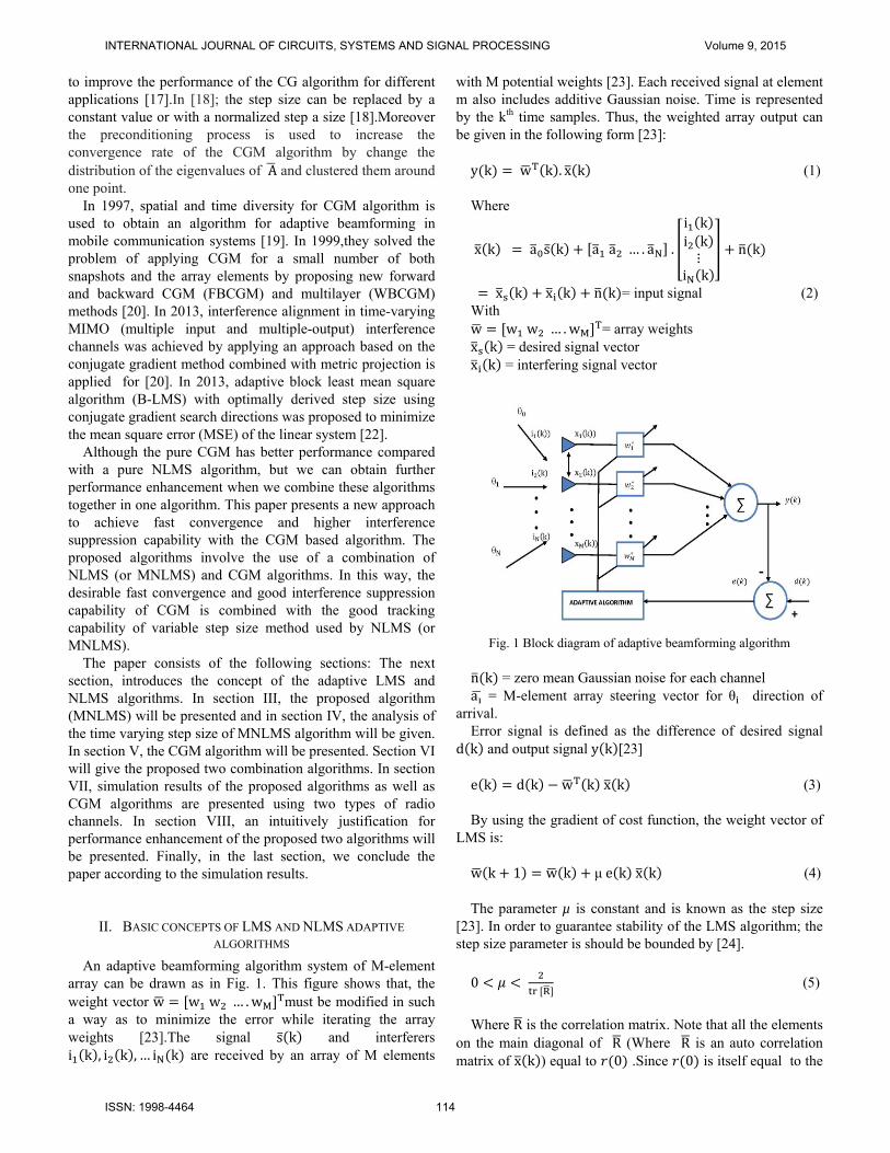
An adaptive beamforming algorithm system of M-element array can be drawn as in Fig. 1. This figure shows that, the weight vector w w w … .w must be modified in such a way as to minimize the error while iterating the array weights [23].The signal s k and interferers i k , i k , … i k are received by an array of M elements

with M potential weights [23]. Each received signal at element m also includes additive Gaussian noise. Time is represented by the kth time samples. Thus, the weighted array output can be given in the following form [23]:

y k w k . x k (1) Where

x k a s k a a … . a .

i ki k⋮

i k

n k

x k x k n k = input signal (2) With w w w … .w = array weights x k = desired signal vector x k = interfering signal vector

Fig. 1 Block diagram of adaptive beamforming algorithm n k = zero mean Gaussian noise for each channel a = M-element array steering vector for θ direction of

arrival. Error signal is defined as the difference of desired signal

d k and output signal y k [23] e k d k w k x k (3) By using the gradient of cost function, the weight vector of

LMS is: w k 1 w k μe k x k (4) The parameter µ is constant and is known as the step size

[23]. In order to guarantee stability of the LMS algorithm; the step size parameter is should be bounded by [24].

0

(5)

Where R is the correlation matrix. Note that all the elements

on the main diagonal of R (Where R is an auto correlation matrix of x k ) equal to 0 .Since 0 is itself equal to the


ISSN: 1998-4464 114

mean square value of the input at each of the M- taps in FIR filter, then tr R Mr 0 (6) The LMS algorithm uses a constant step size μ proportional

to the stability bound:

(7)

Since knowledge of the signal statistic 0 is not available, a temporary estimate of the 0 can be computed by:-

0 x x ) (8)

Then the “normalized” is given by

(9)

This is the upper limit of step size, therefore, the practical equation for the step size used for NLMS is [24]:

(10)

Where is a small positive constant and should be bound to guarantee the convergence of the NLMS algorithm [24],

w k 1 w kμ

‖ ‖e k x k (11)

Where ‖x ‖ x x The fixed regularization parameter 0 is added to

overcome the problem of dividing by small value for the x x [23].

III. MODIFIED NORMALIZED LEAST MEAN SQUARE ALGORITHM

(MNLMS)

The proposed MNLMS algorithm introduces a new way of choosing the step size. The small constant in the NLMS algorithm has fixed effect in step size update parameter and may cause a reduction in its value. This reduction in step size affects the convergence rate and weight stability of the NLMS algorithm. In MNLMS algorithm, the error signal may be used to avoid denominator being zero and to control the step size in each iteration. According to this approach, the parameter can be set as:

(12)

The proposed new step size formula can be written as

‖ ‖ (13)

Clearly, is controlled by normalization of both reciprocal of the squared of the estimation error and the input data vector. Therefore, the weight vector of MNLMS algorithm is w 1 w

‖ ‖x (14)

As can be seen from (13), the step size of MNLMS reduces

and increases according to the reciprocal of the squared estimation error and input tap vectors.

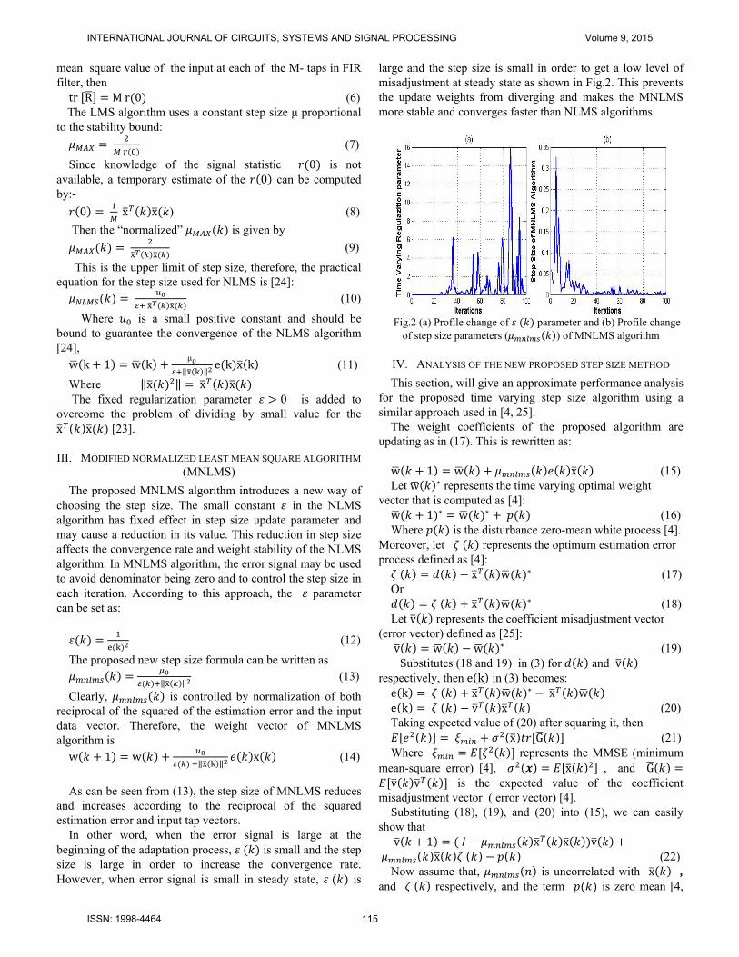
In other word, when the error signal is large at the beginning of the adaptation process, is small and the step size is large in order to increase the convergence rate. However, when error signal is small in steady state, is

large and the step size is small in order to get a low level of misadjustment at steady state as shown in Fig.2. This prevents the update weights from diverging and makes the MNLMS more stable and converges faster than NLMS algorithms.

Fig.2 (a) Profile change of parameter and (b) Profile change

of step size parameters ( ) of MNLMS algorithm

IV. ANALYSIS OF THE NEW PROPOSED STEP SIZE METHOD

This section, will give an approximate performance analysis for the proposed time varying step size algorithm using a similar approach used in [4, 25].

The weight coefficients of the proposed algorithm are updating as in (17). This is rewritten as:

w 1 w x (15) Let w ∗ represents the time varying optimal weight

vector that is computed as [4]: w 1 ∗ w ∗ (16) Where is the disturbance zero-mean white process [4].

Moreover, let represents the optimum estimation error process defined as [4]:

x w ∗ (17) Or

x w ∗ (18) Let v represents the coefficient misadjustment vector

(error vector) defined as [25]: v w w ∗ (19) Substitutes (18 and 19) in (3) for and v

respectively, then e k in (3) becomes: e k x w ∗ x w e k v x (20) Taking expected value of (20) after squaring it, then

x G (21) Where represents the MMSE (minimum

mean-square error) [4], x , and Gv v is the expected value of the coefficient

misadjustment vector ( error vector) [4]. Substituting (18), (19), and (20) into (15), we can easily

show that v 1 x x v

x (22) Now assume that, is uncorrelated with x ,

and respectively, and the term is zero mean [4,


ISSN: 1998-4464 115

16], then the expected value of the weight vector is given by [4]:

v 1 x x v (23)

Then the convergence of the proposed algorithm is guaranteed if the expected value of the step size parameter is within the following bound: 0 2 (24)

V. CONJUGATE GRADIENT METHOD (CGM)

The goal of CGM algorithm is to iteratively search for the optimum solution by choosing conjugate (perpendicular) paths for each new iteration [24]. CGM is an iterative method whose goal is to minimize the quadratic cost function [24]

(25)

Where A is the K x M matrix of array snapshots, (K = number of snapshots and M = number of array elements). d d 1 d 2 … . d K is the desired signal vector of K snapshots. It can be shown that the gradient of the cost function is [24]:

(26)

Starting with an initial guess for the weightsw 1 , then the first residual value r 1 after at the first guess (iteration =1) is given as [24]:

1 1 1 (27)

The new conjugate direction vector D to iterate toward the optimum weight is [24]:

1 1 (28)

The general weight update expression is given by [24]:

1 μ (29) Where µ is the step-size of CGM and is given by [24]:

μ

(30)

The residual vector update is given by [24]: 1 μ (31)

and the direction vector update is given by [24]:

1 1 (32) A linear search is used to determine α (k) which

minimizes w k .

(33)

Thus, the procedure to use CGM is to find the residual and the corresponding weights and update until convergence is satisfied.

VI. THE PROPOSED NLMS-CGM AND MNLMS-CGM

ALGORITHMS

The convergence rate for CGM can be accelerated and the mean square error (MSE) can be minimized by use of different techniques. One such technique is combining more than one algorithm. This paper proposes an algorithm that uses a combination of the gradient based directions with conjugate gradient based directions. The two proposed algorithms can summarized as the following

1. The first proposed algorithm is called NLMS-CGM which is a combination of NLMS and CGM algorithms. The CGM algorithm uses the weight vector that calculated by the NLMS algorithm as initial value to calculate the final optimal weight.

2. The second proposed algorithm is called MNLMS-CGM. It makes use of two individual algorithm stages, based on the proposed MNLMS and CGM algorithms.

With the proposed (NLMS-CGM) and (MNLMS-CGM) algorithms scheme, the estimated weight coefficients, obtained from the first NLMS or MNLMS algorithm, is storage, and then they used as initial weight coefficients for CGM algorithm processing. In this way, the CGM weight coefficients will not be initiated with zero value but with previously estimated values that are obtained from the first algorithm (NLMS or MNLMS). Table 1 shows the step sequence for both proposed algorithms.

VII. SIMULATION RESULTS

In this section, the pure CGM and pure NLMS are first tested in order to evaluate their performance without combination process .Then NLMS-CSM and MNLMS-CGM algorithms are evaluated and simulated for smart antenna applications.

For the purpose of illustration and comparison, in all simulations presented here, a linear array consisting of M= 10 isotropic elements with d 0.5λ element spacing is used under the following conditions.

Input signal S k cos 2πft k with f 900

MHZ andt 1: k ∗ T/k where k is the number of sample intervals and T is the time period. Desired ( Angle of Arrival) AOA of θ 0 and two

interfering signals, i1 and i2 with two AOA’s, θ45 , θ 30 . All weight vectors are initially set to zero. Desired signald k S k . Initial step size parameter µ 1

Regularization parameter ( ) for NLMS is set to 1e-12. Zero mean Gaussian noise with variance σ 0. 001 is

added to the input signal for each element in the array. Signal to Noise ratio (SNR) is set to 30 dB, and Signal to

Interference ration (SIR) is set to 10 dB.


ISSN: 1998-4464 116

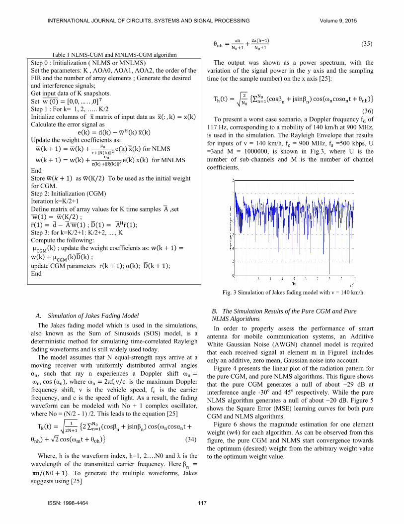
Table 1 NLMS-CGM and MNLMS-CGM algorithm Step 0 : Initialization ( NLMS or MNLMS) Set the parameters: K , AOA0, AOA1, AOA2, the order of the FIR and the number of array elements ; Generate the desired and interference signals; Get input data of K snapshots. Set w 0 0,0, … . . ,0 Step 1 : For k= 1, 2, ….. K/2 Initialize columns of x matrix of input data as x : , k x k Calculate the error signal as

e k d k w k x k Update the weight coefficients as: w k 1 w k

μ

‖ ‖e k x k for NLMS

w k 1 w k ‖ ‖

e k x k for MNLMS

End Store w 1 as w K/2 To be used as the initial weight for CGM. Step 2: Initialization (CGM) Iteration k=K/2+1 Define matrix of array values for K time samples A ,set w 1 w K/2 ; r 1 d Aw 1 ; D 1 A r 1 ; Step 3: for k=K/2+1: K/2+2, ...., K Compute the following: µ k ; update the weight coefficients as: w k 1w k µ k D k ; update CGM parameters r k 1 ; α k ; D k 1 ; End

A. Simulation of Jakes Fading Model

The Jakes fading model which is used in the simulations, also known as the Sum of Sinusoids (SOS) model, is a deterministic method for simulating time-correlated Rayleigh fading waveforms and is still widely used today.

The model assumes that N equal-strength rays arrive at a moving receiver with uniformly distributed arrival angles α , such that ray n experiences a Doppler shift ωω cos α , where ω 2πf v/c is the maximum Doppler frequency shift, v is the vehicle speed, f is the carrier frequency, and c is the speed of light. As a result, the fading waveform can be modeled with No + 1 complex oscillator, where No = (N/2 - 1) /2. This leads to the equation [25]

T t 2∑ cosβ jsinβ cos ω cosα t

θ √2 cos ω t θ (34) Where, h is the waveform index, h=1, 2….N0 and λ is the

wavelength of the transmitted carrier frequency. Hereβ πn/ N0 1 . To generate the multiple waveforms, Jakes suggests using [25]

θπ π

(35)

The output was shown as a power spectrum, with the

variation of the signal power in the y axis and the sampling time (or the sample number) on the x axis [25]:

T t ∑ cosβ jsinβ cos ω cosα t θ

(36) To present a worst case scenario, a Doppler frequency f of

117 Hz, corresponding to a mobility of 140 km/h at 900 MHz, is used in the simulation. The Rayleigh Envelope that results for inputs of v = 140 km/h, f = 900 MHz, f =500 kbps, U =3and M = 1000000, is shown in Fig.3, where U is the number of sub-channels and M is the number of channel coefficients.

Fig. 3 Simulation of Jakes fading model with v = 140 km/h.

B. The Simulation Results of the Pure CGM and Pure NLMS Algorithms

In order to properly assess the performance of smart antenna for mobile communication systems, an Additive White Gaussian Noise (AWGN) channel model is required that each received signal at element m in Figure1 includes only an additive, zero mean, Gaussian noise into account.

Figure 4 presents the linear plot of the radiation pattern for the pure CGM, and pure NLMS algorithms. This figure shows that the pure CGM generates a null of about −29 dB at interference angle -30o and 45o respectively. While the pure NLMS algorithm generates a null of about −20 dB. Figure 5 shows the Square Error (MSE) learning curves for both pure CGM and NLMS algorithms.

Figure 6 shows the magnitude estimation for one element weight (w4) for each algorithm. As can be observed from this figure, the pure CGM and NLMS start convergence towards the optimum (desired) weight from the arbitrary weight value to the optimum weight value.


ISSN: 1998-4464 117

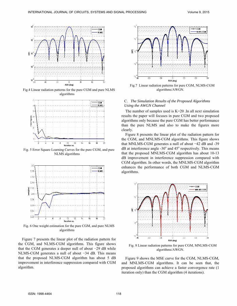
Fig.4 Linear radiation patterns for the pure CGM and pure NLMS

algorithms

Fig. 5 Error Square Learning Curves for the pure CGM, and pure

NLMS algorithms

Fig. 6 One weight estimation for the pure CGM, and pure NLMS

algorithms Figure 7 presents the linear plot of the radiation pattern for

the CGM, and NLMS-CGM algorithms. This figure shows that the CGM generates a deeper null of about −29 dB while NLMS-CGM generates a null of about −34 dB. This means that the proposed NLMS-CGM algorithm has about 5 dB improvement in interference suppression compared with CGM algorithm.

Fig.7 Linear radiation patterns for pure CGM, NLMS-CGM

algorithms/AWGN.

C. The Simulation Results of the Proposed Algorithms Using the AWGN Channel

The number of samples used is K=20 .In all next simulation results the paper will focuses in pure CGM and two proposed algorithms only because the pure CGM has better performance than the pure NLMS and also to make the figures more clearly.

Figure 8 presents the linear plot of the radiation pattern for the CGM, and MNLMS-CGM algorithms. This figure shows that MNLMS-CGM generates a null of about −42 dB and -39 dB at interference angle -30o and 45o respectively. This means that the proposed MNLMS-CGM algorithm has about 10-13 dB improvement in interference suppression compared with CGM algorithm. In other words, the MNLMS-CGM algorithm enhances the performance of both CGM and NLMS-CGM algorithms.

Fig. 8 Linear radiation patterns for pure CGM, MNLMS-CGM

algorithms/AWGN.

Figure 9 shows the MSE curve for the CGM, NLMS-CGM, and MNLMS-CGM algorithms. It can be seen that, the proposed algorithms can achieve a faster convergence rate (1 iteration only) than the CGM algorithm (4 iterations).


ISSN: 1998-4464 118

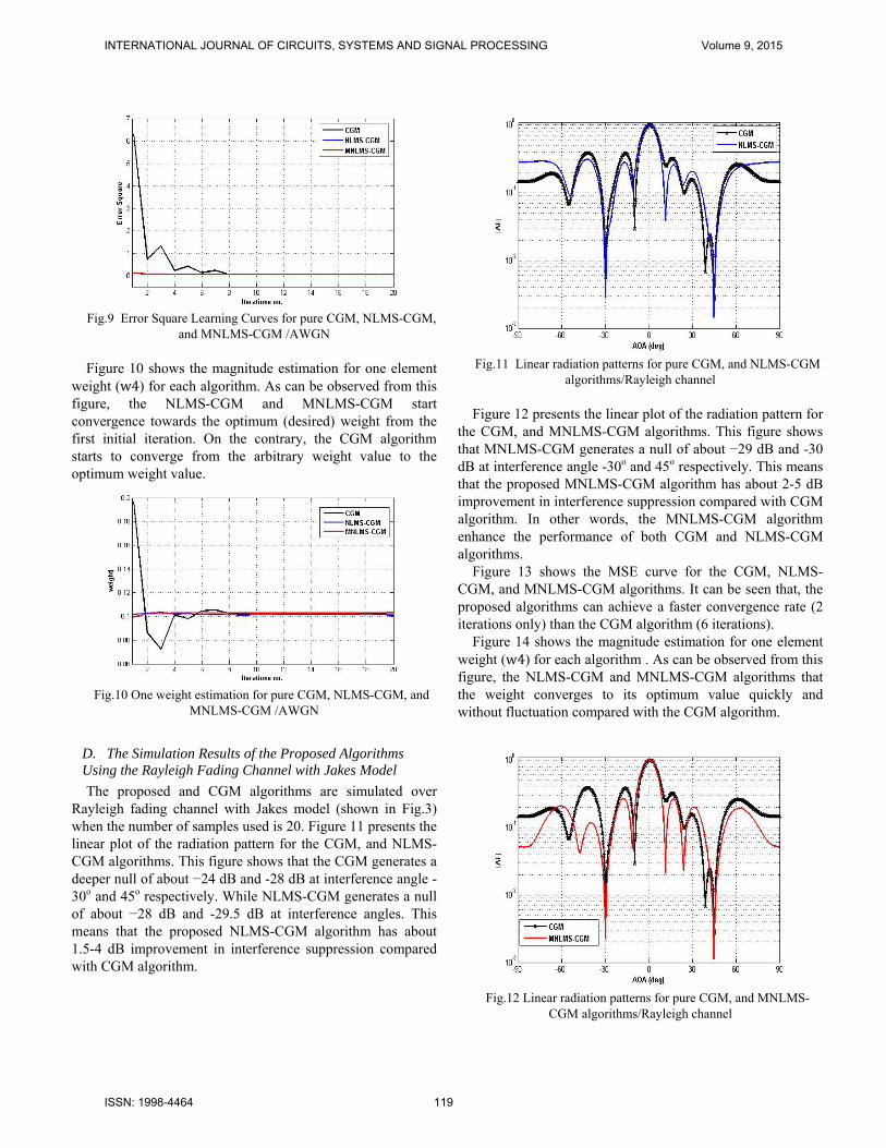
Fig.9 Error Square Learning Curves for pure CGM, NLMS-CGM,

and MNLMS-CGM /AWGN

Figure 10 shows the magnitude estimation for one element weight (w4) for each algorithm. As can be observed from this figure, the NLMS-CGM and MNLMS-CGM start convergence towards the optimum (desired) weight from the first initial iteration. On the contrary, the CGM algorithm starts to converge from the arbitrary weight value to the optimum weight value.

Fig.10 One weight estimation for pure CGM, NLMS-CGM, and

MNLMS-CGM /AWGN

D. The Simulation Results of the Proposed Algorithms Using the Rayleigh Fading Channel with Jakes Model

The proposed and CGM algorithms are simulated over Rayleigh fading channel with Jakes model (shown in Fig.3) when the number of samples used is 20. Figure 11 presents the linear plot of the radiation pattern for the CGM, and NLMS-CGM algorithms. This figure shows that the CGM generates a deeper null of about −24 dB and -28 dB at interference angle -30o and 45o respectively. While NLMS-CGM generates a null of about −28 dB and -29.5 dB at interference angles. This means that the proposed NLMS-CGM algorithm has about 1.5-4 dB improvement in interference suppression compared with CGM algorithm.

Fig.11 Linear radiation patterns for pure CGM, and NLMS-CGM

algorithms/Rayleigh channel Figure 12 presents the linear plot of the radiation pattern for

the CGM, and MNLMS-CGM algorithms. This figure shows that MNLMS-CGM generates a null of about −29 dB and -30 dB at interference angle -30o and 45o respectively. This means that the proposed MNLMS-CGM algorithm has about 2-5 dB improvement in interference suppression compared with CGM algorithm. In other words, the MNLMS-CGM algorithm enhance the performance of both CGM and NLMS-CGM algorithms.

Figure 13 shows the MSE curve for the CGM, NLMS-CGM, and MNLMS-CGM algorithms. It can be seen that, the proposed algorithms can achieve a faster convergence rate (2 iterations only) than the CGM algorithm (6 iterations).

Figure 14 shows the magnitude estimation for one element weight (w4) for each algorithm . As can be observed from this figure, the NLMS-CGM and MNLMS-CGM algorithms that the weight converges to its optimum value quickly and without fluctuation compared with the CGM algorithm.

Fig.12 Linear radiation patterns for pure CGM, and MNLMS-

CGM algorithms/Rayleigh channel


ISSN: 1998-4464 119

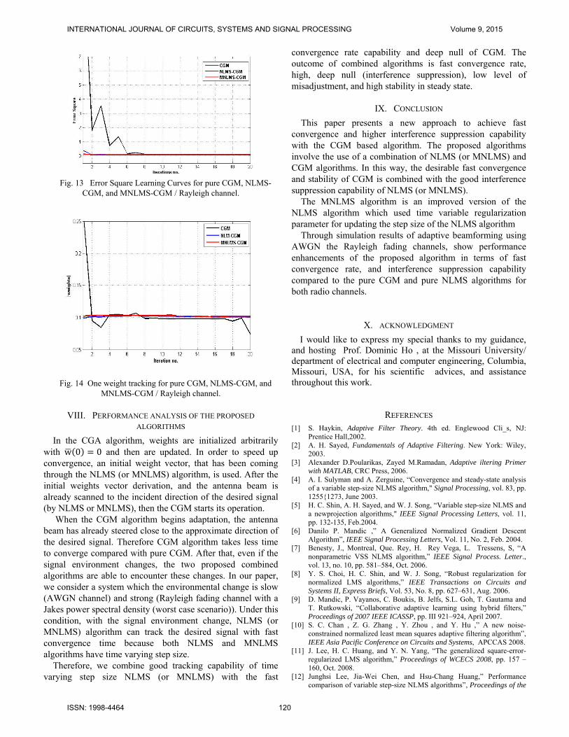
Fig. 13 Error Square Learning Curves for pure CGM, NLMS-

CGM, and MNLMS-CGM / Rayleigh channel.

Fig. 14 One weight tracking for pure CGM, NLMS-CGM, and MNLMS-CGM / Rayleigh channel.

VIII. PERFORMANCE ANALYSIS OF THE PROPOSED

ALGORITHMS

In the CGA algorithm, weights are initialized arbitrarily with w 0 0 and then are updated. In order to speed up convergence, an initial weight vector, that has been coming through the NLMS (or MNLMS) algorithm, is used. After the initial weights vector derivation, and the antenna beam is already scanned to the incident direction of the desired signal (by NLMS or MNLMS), then the CGM starts its operation.

When the CGM algorithm begins adaptation, the antenna beam has already steered close to the approximate direction of the desired signal. Therefore CGM algorithm takes less time to converge compared with pure CGM. After that, even if the signal environment changes, the two proposed combined algorithms are able to encounter these changes. In our paper, we consider a system which the environmental change is slow (AWGN channel) and strong (Rayleigh fading channel with a Jakes power spectral density (worst case scenario)). Under this condition, with the signal environment change, NLMS (or MNLMS) algorithm can track the desired signal with fast convergence time because both NLMS and MNLMS algorithms have time varying step size.

Therefore, we combine good tracking capability of time varying step size NLMS (or MNLMS) with the fast

convergence rate capability and deep null of CGM. The outcome of combined algorithms is fast convergence rate, high, deep null (interference suppression), low level of misadjustment, and high stability in steady state.

IX. CONCLUSION

This paper presents a new approach to achieve fast convergence and higher interference suppression capability with the CGM based algorithm. The proposed algorithms involve the use of a combination of NLMS (or MNLMS) and CGM algorithms. In this way, the desirable fast convergence and stability of CGM is combined with the good interference suppression capability of NLMS (or MNLMS).

The MNLMS algorithm is an improved version of the NLMS algorithm which used time variable regularization parameter for updating the step size of the NLMS algorithm

Through simulation results of adaptive beamforming using AWGN the Rayleigh fading channels, show performance enhancements of the proposed algorithm in terms of fast convergence rate, and interference suppression capability compared to the pure CGM and pure NLMS algorithms for both radio channels.

X. ACKNOWLEDGMENT

I would like to express my special thanks to my guidance, and hosting Prof. Dominic Ho , at the Missouri University/ department of electrical and computer engineering, Columbia, Missouri, USA, for his scientific advices, and assistance throughout this work.

REFERENCES [1] S. Haykin, Adaptive Filter Theory. 4th ed. Englewood Cli_s, NJ:

Prentice Hall,2002. [2] A. H. Sayed, Fundamentals of Adaptive Filtering. New York: Wiley,

2003. [3] Alexander D.Poularikas, Zayed M.Ramadan, Adaptive iltering Primer

with MATLAB, CRC Press, 2006. [4] A. I. Sulyman and A. Zerguine, “Convergence and steady-state analysis

of a variable step-size NLMS algorithm," Signal Processing, vol. 83, pp. 1255{1273, June 2003.

[5] H. C. Shin, A. H. Sayed, and W. J. Song, “Variable step-size NLMS and a newprojection algorithms," IEEE Signal Processing Letters, vol. 11, pp. 132-135, Feb.2004.

[6] Danilo P. Mandic ,” A Generalized Normalized Gradient Descent Algorithm”, IEEE Signal Processing Letters, Vol. 11, No. 2, Feb. 2004.

[7] Benesty, J., Montreal, Que. Rey, H. Rey Vega, L. Tressens, S, “A nonparametric VSS NLMS algorithm,” IEEE Signal Process. Letter., vol. 13, no. 10, pp. 581–584, Oct. 2006.

[8] Y. S. Choi, H. C. Shin, and W. J. Song, “Robust regularization for normalized LMS algorithms,” IEEE Transactions on Circuits and Systems II, Express Briefs, Vol. 53, No. 8, pp. 627–631, Aug. 2006.

[9] D. Mandic, P. Vayanos, C. Boukis, B. Jelfs, S.L. Goh, T. Gautama and T. Rutkowski, “Collaborative adaptive learning using hybrid filters,” Proceedings of 2007 IEEE ICASSP, pp. III 921–924, April 2007.

[10] S. C. Chan , Z. G. Zhang , Y. Zhou , and Y. Hu ,” A new noise-constrained normalized least mean squares adaptive filtering algorithm”, IEEE Asia Pacific Conference on Circuits and Systems, APCCAS 2008.

[11] J. Lee, H. C. Huang, and Y. N. Yang, “The generalized square-error-regularized LMS algorithm,” Proceedings of WCECS 2008, pp. 157 – 160, Oct. 2008.

[12] Junghsi Lee, Jia-Wei Chen, and Hsu-Chang Huang,” Performance comparison of variable step-size NLMS algorithms”, Proceedings of the


ISSN: 1998-4464 120

World Congress on Engineering and Computer Science Vol. I , San Francisco, USA , October 20-22, 2009.

[13] Junghsi Lee, Hsu Chang Huang, Yung Ning Yang, and Shih Quan Huang,” A Square-Error-Based Regularization for Normalized LMS Algorithms”, Proceedings of the International MultiConference of Engineers and Computer Scientists Vol. II ,19-21, Hong Kong, March, 2008.

[14] Zayed Ramadan,” Error Vector Normalized Adaptive Algorithm Applied to Adaptive Noise Canceller and System Identification” American J. of Engineering and Applied Sciences 3 (4): 710-717, 2010

[15] Hsu-Chang Huang and Junghsi Lee,” A new variable step-size NLMS algorithm and its performance analysis”, IEEE transaction on Signal Processing, Vol. 60, No. 4, April, 2012.

[16] Shengyu Wang, Hong Mi, Bin Xi, Daniel(Jian) Sun,” Conjugate Gradient-based Parameters Identification”, 2010 8th IEEE International Conference on Control and Automation , Xiamen, China, pp 1071-1075, June 9-11, 2010.

[17] Pi Sheng Chang, and Alan N. Willson, Jr.,” Analysis of Conjugate Gradient Algorithms for Adaptive Filtering”, IEEE Transaction on signal processing, VOL. 48, NO. 2, pp 409-418 , FEBRUARY 2000.

[18] G. K. Boray, M. D. Srinath, “Conjugate Gradient Techniques for Adaptive Filtering”, IEEE Trans. on Circ. And Sys. Vol. CAS-1, pp. 1-10, Jan. 1992.

[19] Mandyam, G.D. ; Ahmed, N. ; Srinath, M.D. , “Adaptive Beamforming Based on the Conjugate Gradient Algorithm”, IEEE Transactions on Aerospace and Electronic Systems, Volume: 33 , Issue: 1 , Page(s): 343 – 347, 1997.

[20] Tang Jun * Peng Yingning Wang Xiqin,” Application of Conjugate Gradient Algorithm to Adaptive Beamforming”, International Symposium on Antennas and Propagation Society, Orlando, FL, USA , Page(s): 1460 - 1463 vol.2 1999.

[21] Junse Lee, Heejung Yu, and Youngchul Sung,” Beam Tracking for Interference Alignment in Time-Varying MIMO Interference Channels: A Conjugate Gradient Based Approach”, Final Version Submitted to IEEE Trans. on Vehicular Technology, August 20, 2013.

[22] Syed Alam Abbas,” A New Fast Algorithm to Estimate Real-Time Phasors Using Adaptive Signal Processing”, IEEE Trans. On Power Delivery, VOL. 28, NO. 2, pp 807- 815, APRIL 2013.

[23] Gross, F. B., Smart Antenna for Wireless Communication, McGraw-Hill, Inc, USA, 2005.

[24] J. Mathews and Z. Xie. " A stochastic gradient adaptive filter with gradient adaptive step size", IEEE transaction on signal processing , 41(6), pp.2075-2087, 1993.

[25] Vanderlei A. Silva, Taufik Abrao, and Paul Jean E. Jeszensky, “Statistically correct simulation models for the generation of multiple uncorrelated rayleigh fading waveforms”, IEEE Eighth International Symposium on Spread Spectrum Techniques and Applications, Sydney, Australia, 30 Aug. - 2 Sep. 2004.

Thamer M. Jamel was born in Baghdad, Iraq in 1961. He graduated from the University of Technology with a Bachelor's degree in electronics engineering in 1983. He received a Master's degree in digital communications engineering from the University of Technology in 1990 and a Doctoral degree in communication engineering from the University of Technology in 1997. He is an associate professor in the communication engineering branch, Electrical engineering department at University of Technology, Baghdad, Iraq. Currently, he is a visitor scholar in the electrical and computer engineering department at University of Missouri, Columbia, USA. His research interests include adaptive signal processing, Neural Networks, DSP microprocessors, FPGA, and Modern digital communications systems.


ISSN: 1998-4464 121

Performance Enhancement of Conjugate Gradient Method (CGM ...

Documents

Transcript of Performance Enhancement of Conjugate Gradient Method (CGM ...