A conjugate Rosen’s gradient projection method withglobal line search for piecewise linear optimization∗

C. Beltran-Royo†

July 18, 2005

Abstract

The Kelley cutting plane method is one of the methods commonly used to op-timize the dual function in the Lagrangian relaxation scheme. Usually the Kelleycutting plane method uses the simplex method as the optimization engine. It is wellknown that the simplex method leaves the current vertex, follows an ascending edgeand stops at the nearest vertex. What would happen if one would continue the linesearch up to the best point instead? As a possible answer, we propose theface sim-plex method, which freely explores the polyhedral surface by following the Rosen’sgradient projection combined with aglobal line search on the whole surface. Fur-thermore, to avoid the zig-zagging of the gradient projection, we propose a conjugategradient version of the face simplex method. We have implemented this method inMatlab. This implementation clearly outperforms basic Matlab implementations ofthe simplex method. In the case of state-of-the-art simplex implementations in C,our Matlab implementation is only competitive for the case of many cutting planes.

Keywords: Linear programming, Kelley cutting plane method, simplex method,Rosen’s gradient projection, conjugate gradient.

1 Introduction

The objective of this paper is to explore the computational performance of theface simplex (FS)method as a procedure to maximize an unconstrainedpiecewise linear concave (PLC) function,in the framework of the Kelley cutting plane method [14]. In the remaining of the paper cuttingplane method will refer to the Kelley cutting plane method. Our purpose is not to compare thecutting plane method, to other methods used to maximize the Lagrangian dual function as forexample: bundle methods [12], ACCPM (analytic center cutting plane method) [1], subgradientmethods [21], etc. Instead, we are interested in comparing two optimization tools to be usedwithin the cutting plane framework: the simplex and the FS method.

PLC functions are nondifferentiable and arise in the frame of the cutting plane method usedfor example to maximize the (Lagrangian) dual function [4]. The dual function is concave and

∗This work was partially supported by Logilab, HEC, University of Geneva and the Spanish government, MCYTsubsidy dpi2002-03330.

†cesar.beltran@hec.unige.ch, Logilab, HEC, University of Geneva, Switzerland.

1

very often not explicitly known. For this reason, first order information of the dual function(cutting planes) is gathered by means of black-box procedures also called oracles. The cumu-lated set of cutting planes constitutes a PLC outer approximation to the unknown dual function.At each cutting plane iteration one maximizes and improves this PLC approximation to the dualfunction.

The FS method is an alternative to the simplex method to maximize a PLC function. It hastwo inherent advantages: First, the FS method does not need the expensive initialization of thesimplex method (to find an initial vertex). Second, in the case of a PLC unconstrained function,it may happen that there is no optimal vertex. In contrast with the FS method, the simplexmethod simply will either not be able to optimize such a function or will need to bound thevariables in an artificial way, if possible.

It is well known that the simplex method at the current vertex takes an ascending edge andstops at the other vertex of the edge.Question I: What would happen if instead of stopping theline search at the second vertex, one continues the line search on the whole PLC surface up tothe best point? Firstly, we would obtain a point at least as good as the one given by the simplexmethod in terms of objective value. Secondly, most probably the next iterate would not be avertex any more and therefore the ascending edge direction proposed by the simplex methodwould not exist at this point. In this situation, the FS method proposes to follow the Rosen’sgradient projection direction [19].

However, while the Rosen’s gradient projection method performs alocal line search (withinthe current face of the associated polyhedron), the FS method performs aglobal line search onthe whole polyhedral surface. Both simplex and FS method use the Rosen’s gradient projectionas the feasible direction. They differ on the line search. In fact, the simplex method has the samebehavior as the Rosen’s gradient projection method started at a vertex (except for streamliningthe linear algebra) [4].

Numerous gradient-like methods have been proposed to solve linear programs. In fact theyappeared at the same time as the simplex method [5]. Later references are the Zoutendijk’smethod of feasible directions [25], the already mentioned Rosen’s projected gradient methodand the constrained gradient method [15], among others. More recently the steepest descentgravitational method has been proposed [6].

Two main aspects determine a gradient projection method. The direction search and the linesearch. Regarding the direction search, we also encounter two principal approaches: projectionof the gradient on the entire polyhedral surface, not to be mistaken with the projection of thegradient on the current face (here we are assuming than all the problem constraints are linear).We will use the termsgradient projection for the first case andRosen’s gradient projection forthe second one. Regarding the line search, we also encounter two principal approaches: linesearch on the current face and line search on the whole polyhedral surface. We will use thetermslocal line search andglobal line search, respectively.

The gradient projection method has guaranteed convergence for both local and global linesearch. But, it requires the solving of a demanding quadratic programming problem in order toproject the gradient on the constraint surface. Closely related to the gradient projection, there isthe steepest ascent method [12], which also requires to solve a quadratic programming problemat each iteration. It has guaranteed convergence only for local line search. If one wishes toperform long steps (global line search) along anapproximate steepest ascent, one has to use anouter approximate subdifferential instead of the pure subdifferential [18].

2

In contrast, the computation of the Rosen’s gradient projection is far less demanding sinceit only requires the product of the gradient by a projection matrix [4]. In this case we have thesteepest ascenton the current face. In [7], the Rosen’s gradient projection is used in combinationwith local line search to solve the uncapacitated facility location problem. The global line searchcombined with the gradient projection has been used in [10] to solve the graph partitioningproblem. To our knowledge the combination of the Rosen’s gradient projection with a globalline search has never been used. The FS method fills this gap and constitutes a possible answerto above Question I.

A second issue addressed in this paper is the zig-zagging inherent to gradient like methods.In the differentiable case the zig-zagging is addressed by the conjugate gradient or equivalently,by the partan method [16]. Here we adapt to the case of a PLC function, the partan method.In our nondifferentiable problem the partan method is used only as a strategy to deflect theprojected gradient, in contrast with the differentiable case where some conjugacy requirementis enforced. Conjugate subgradient methods have already been used toapproximately solvenondifferentiable problems [23, 8]. Here, the partan FS method will compute anexact optimumof the PLC function.

This paper is organized as follows. In section 2 we state the PLC problem and associatednotation. In section 3 the FS method is introduced. The global line search by the radar methodis presented in section 4. A short discussion on the convergence of the FS method is presentedin section 5. The partan FS method is introduced in section 6. Finally the numerical tests andconclusions can be found in sections 7 and 8, respectively.

2 Statement of the problem and notation

In the cutting plane method we generate a set of hyperplanes (cuts){πj ≡ z = s′jy+bj}j∈J withJ = {1, . . . ,m} whose lower envelope describes a piecewise linear concave (PLC) function:

F (y) = min{Fj(y) | j ∈ J},

whereFj(y) = s′jy + bj .

At each iteration of the cutting plane method one maximizesF (we call it thePLC problem):

maxy∈Rn−1

F (y). (1)

This problem can be rewritten as:

z∗ = max(y,z)∈Rn

{z | z ≤ s′jy + bj , j ∈ J}. (2)

By definingx = (y, z) ∈ Rn−1 × R1, aj = (−sj , 1) andG(x) = z, the PLC problem isequivalent to:

maxx∈Rn{G(x) | a′jx ≤ bj , j ∈ J} =maxx∈Rn{G(x) | Ax ≤ b}. (3)

Therefore the PLC can be seen as the unrestricted maximization of the (nonsmooth) PLCfunctionF (y) in they-space (formulation (1)) or as the constrained maximization of the (smooth)linear functionG(x) in the enhancedx-space (formulation (3)).

3

The notation is as follows:

αk denotes thekth term of the sequence{αk},

(α)k to write a power we use parenthesis,

xi ith component of vectorx,

x = (y, z) ∈ Rn−1 ×R1, partition ofx into ground variables y andepigraph variable z,

ProjE(·) Orthogonal projection onto the spaceE,

Projy(·) Orthogonal projection onto the firstn− 1 coordinate space, e.g., Projy(x) = y,

gk = ∇G(xk),

en = (0, . . . , 0, 1) nth canonical vector ofRn ,

J(x) = {j ∈ J | a′jx = bj} active index-set associated to the active constraints atx,

Jk = J(xk),

Jk \ h = Jk \ {h} set difference,

AJ sub matrix ofA with rows indexed byJ,

Ak = AJk ,

bk = bJk ,

Sk = {x ∈ Rn | Akx = bk} active linear manifold atxk,

Ek = {x ∈ Rn | Akx = 0} vector space associated toSk,

Sky = Projy(S

k),

Eky = Projy(E

k),

X = {x ∈ Rn | Ax ≤ b},

FS Face simplex,

PLC Piecewise linear concave.

Assumption 1: {aj}j∈J(x) is a set of independent vectors for anyx ∈ Rn.

Assumption 2: The PLC problem is bounded (z∗ < ∞).

4

3 The face simplex method

The face simplex (FS) method is intended to solve the PLC problem (3) and ‘only’ differs fromthe Rosen’s gradient projection method in the scope of the line search (see Remark 1 c)). TheFS method can be summarized as follows:

Face simplex method:

Step 0. Initialization: Takex0 ∈ X such thatJ(x0) 6= ∅, ε > 0 and setk = 0.

Step 1. Compute the Rosen’s gradient projection:

Jk = J(xk),

P k = I −Ak ′(AkAk ′)−1Ak,

ukj = (AkAk ′)−1Akgk, j ∈ Jk,

ukh = min{uk

j | j ∈ Jk}.

If ‖P kgk‖ < ε andukh ≥ 0 then stop (in this casexk is a Karush-Kunhn-Tucker point),

else, choose

dk ={

P kgk if ‖P kgk‖ > ukhε,

PJk\hgk if ‖P kgk‖ ≤ ukhε,

(4)

wherePJk\h = I −A′Jk\h(AJk\hA′

Jk\h)−1AJk\h.

Step 2. Global line search along dky = Projy(d

k):

xk+1 = (yk+1, zk+1) = arg max zs.t. (y, z) ∈ X ∩Hk,

(5)

whereHk = xk + span{dk

y , en}.

Setk = k + 1 and go back to Step 1.

Remark 1 a) Note thatgk = (0, . . . , 0, 1) = en for all x ∈ Rn. Then in the previous algorithmgk = en for all k.

b) The FS method corresponds to the gradient projection method of Rosen with an enlargedlinear manifold at Step 2. That is, in the Rosen’s gradient projection method, the line search isrestricted to the one dimensional linear manifoldHk = xk + span{dk} instead ofHk, which istwo dimensional.

c) The Rosen’s gradient projectiondk corresponds to the steepest ascend directionwithinF k, the face associated toxk in the polyhedronX (except whenF k is a vertex ofX). In arelated method, the steepest ascend method, one computes the (global) steepest ascend directionat xk, which may be different formdk.

5

4 Global line search by the radar method

In this section we focus on the solution of the global line search (5). This problem is equivalentto maximizing a one dimensional PLC functionf(α) since the aim of (5) is to find a highestpoint within a vertical two dimensional slice of the polyhedron X. Furthermoref(α) is the lowerenvelope of the lines{rj(α)}j∈J , whererj(α) = mjα + nj is the equation of the intersectionline of hyperplaneπj with the two dimensional linear manifoldHk. That is

f(α) = min{rj(α) | j ∈ J}.

The expression formj andnj is given in the following lemma.

Lemma 1 If πj ≡ z = s′jy+bj andHk = xk +span{dky , en}, with xk = (yk, zk) ∈ Rn−1×R,

thenπj ∩Hk defines a line whose equation is:

rj(α) = mjα + nj

with mj = s′jdky andnj = s′jy

k + bj .

Proof: Let {(y(α), z(α)) | α ∈ R} be the lineπj ∩ Hk. Sinceπj ≡ z = s′jy + bj andy(α) = yk + αdk

y , then

z(α) = s′jy(α) + bj = αs′jdky + s′jy

k + bj .

The result follows from the fact thatrj(α) is equivalent toz(α).

The global line search (5) can be then reformulated as:

α∗ = argmaxα∈R

f(α) (6)

Without loss of generality, we assume thatα∗ is the smallest optimal point in case of multipleoptima. Furthermore,f is parameterized such thatf(0) = 0 andα∗ > 0. The graph off inthe interval of interestI = [0, α∗] is the union ofr line segments that join the breaking pointspi = (ai, bi) ∈ R2, i = 1, . . . , r. Furthermore,p0 = (0, 0) andpr = (α∗, f(α∗)). The intervalI is partitioned into

I1 ∪ I2 ∪ . . . ∪ Ir = [a0, a1[∪[a1, a2[∪ . . . ∪ [ar−1, ar].

The pointar is characterized as the only point where the left derivative off is strictly positiveand the right derivative is negative, i.e.,f−(ar) > 0 andf+(ar) ≤ 0. This property could beused to solve the global line search: Start ata0 = 0, then iterate from breaking point to breakingpoint up to the first breaking point with a change of sign in the lateral derivatives (next breakingpoint method).

The number of iterations in the next breaking point method equals the number of breakingpoints. To avoid the potentially large number of iterations of the next breaking point method, weuse an improved version of theradar method. Before of introducing the radar method we needto partition the set of lines that definef . We consideractive lines in [0,+∞[ indexed byJa, thatis, lines that intersect with the graph off in more than one point within the interval[0,+∞[.

6

Analogously, we considerinactive lines indexed byJi. We also considerstrictly positive linesindexed byJ+, that is, lines with strictly positive slope. Analogously,negative lines indexed byJ− (negative lines may have null slope). By crossing these two attributes, we partitionJ intofour sets :

J = J+ ∪ J− = J+a ∪ J+

i ∪ J−a ∪ J−

i .

Since in[0, α∗] we haver breaking points, we will haver segments[pi, pi+1[ (i = 0, . . . , r−1). Also, considering that these segments form the graph of a concave function, their slopes willform a decreasing sequence:m1 > m2 > . . . > mr > 0.

At iterationk, the radar method approximatesf(α) by only two of its defining lines:rk(α),andsk(α): rk is the active line atαk (the one with the lowest slope ifαk corresponds to abreaking point) andsk is thestopping line, i.e., the first negative line that intersects withrk asα increases . The intersection point ofrk andsk is the point(αk+1, r(αk+1)), which gives thenext radar iterateαk+1 and an upper bound to the optimal value (r(αk+1) ≥ f(α∗)). See [2]for more details. The radar method can be summarized as follows:

Radar method:

Step 1. Initialization: Takeα0 = 0 and setk = 0.

Step 2. Compute next radar iterate:

αk+1 = min{−mk −mj

nk − nj| j ∈ J−

}. (7)

Step 3. Stopping criterion: If αk+1 = αk, then stop, sinceαk+1 maximizesf(α). Else, set

k = k + 1 and go back to Step 1.

Remark 2 a) A single iteration version of the radar method was first used in [2], thus obtaininga suboptimal solution of the global line search. In this paper, the aim of the radar method is tocompute an optimal solution of the global line search.

b) In [3] it is seen that in order to obtain anε-optimum for the the global line search, i.e., anαε such that|αε − α∗| < ε, the number of radar iterations does not depend on the number ofbreaking points, but on the ratio between the smallest and largest slopes of the positive activelines. That is, for allk:

|αk − α∗| <(

1− mr

m1

)k

|α0 − α∗|’ . (8)

5 Convergence proof inR3

The Rosen’s gradient projection method for linear constraints was first published in 1960 with-out a convergence proof. The mathematical programming community had to wait until 1985 tosee the first convergence proof but only restricted to dimension 3 [24]. Finally, in 1989 Du andZhang [9] gave a general convergence proof.

Similarly, for the FS method we have not yet found a general convergence proof but only aconvergence proof restricted to dimension 3. This simple result encouraged us to keep searching

7

for a general convergence proof and to empirically test the FS method. We wish to point out,that in contrast with the FS method, the steepest ascent method combined with global line searchmay fail to converge to a KKT point even for dimension 3 when maximizing a PLC function,[13].

The following lemma will be used in the proof of the convergence theorem (see [3] for aproof).

Lemma 2 (radar method)

a) If αk ∈ [ai, ai+1[ thenαk+1 ∈ [ai+1, α∗].

b) f(αk+1) > f(αk) for k = 0, 1, . . .

c) G(xk+1) = f(α∗) > f(0) = G(xk) for k = 0, 1, . . .

Theorem 1 The FS method applied to solve the PLC problem inR3 converges to an optimalpoint or detects unboundness ofG(x) after a finite number of iterations.

Proof: The proof is similar to the convergence proof of the simplex method. Now insteadof exploring vertices, the FS method explores vertices and edges. If the polyhedral setX isincluded inR3 then its faces are points, edges or two-dimensional faces. In the radar method,xk+1 is defined by the intersection of two or more lines which correspond to the intersection oftwo or more hyperplanes. This means thatxk+1 is a vertex or lays on an edge. By Lemma 2c) vertices can only be visited once. Again, by Lemma 2 a)-b) an edge can only be visitedonce. Given that the number of vertices and edges is finite, the FS method either will attain amaximum after a finite number of iterations or will encounter an unbounded edge.

6 Avoiding the zig-zagging

Since the FS method is a gradient type method, it can suffer from zig-zagging specially whenthe graph ofF has an ‘elongated’ form. To overcome the zig-zagging, one can use the partan(parallel tangents) method [20], a simple method that is equivalent to the conjugate gradientmethod in the case of a quadratic function. In this section we adapt the partan method to thecase of a PLC function. Note that, in our non differentiable problem, the partan method is onlyused as a strategy to deflect the projected gradient, in contrast with the differentiable case wheresome conjugacy requirement is enforced.

The pure partan method combined with the FS method is as follows. Note that we work onthe ground space variablesy ∈ Rn−1. Start at an arbitraryy0 and computey1 by the FS method.Then at each iterationk ≥ 1 two steps are performed: First, from the pointyk, compute theintermediate pointyk+ 1

2 by the FS method. Second, from the pointyk+ 12 , computeyk+1 as the

best point in the lineL = yk+ 12 + span{yk+ 1

2 − yk−1}. This double step process continues forn− 1 iterations, and then a new partan cycle is restarted with a simple FS step.

Definition 1 Let us define the intervalI(δ) = ]−δ, δ[. Given a functionF (y) : Rn−1 → R, apointy, a directiond and a lineL(y, d) = {y + αd | α ∈ R}, we say thatL is of class:

8

y

y*

a

L(y, a)

Figure 1:

L0, if there existδ > 0 such thatF (y + αd) = F (y) for all α ∈ I(δ).

L+, if there existδ > 0 such thatF (y + αd) > F (y) for someα ∈ I(δ).

L−, if there existδ > 0 such thatF (y + αd) ≤ F (y) for all α ∈ I(δ) andF (y + αd) isnot constant inI(δ).

Example:In Fig. 1, we have the level sets of a PLC function that attains its maximum aty∗. At the pointywe parameterize all the possible search lines by the anglea, i.e., the set of possible search linesis {L(y, a) : a ∈ −[0, π[}. We encounter two types of lines: a) Lines of typeL−: Along theselines any movement fromy does not improve the objective function (a ∈ −[0, π/2]). b) Linesof typeL+: Along these lines we can improve our objective function (a ∈ −]π/2, π[).

In next proposition we see that, all the lines in Projy(Sk), the y-projection of the active

linear manifold at anyxk, are of typeL0 or L+, and thus they are good candidates for searchline spaces.

Proposition 1 If L(yk, dy) is a line included inSky = Projy(S

k), then it is of classL0 or L+.

Proof: By definition of active set, there exitsδ > 0 such thatJ(xk + αd) = J(xk) for allα ∈ I(δ) = ]−δ, δ[ and for alld ∈ Dk = {d ∈ Ek | ‖d‖ = 1}. Then considering thatd = (dy, dz), xk = (yk, zk), we have:

xk + αd ∈ Sk,

yk + αdy ∈ Sky ,

F (yk + αdy) = zk + αdz,

for all α ∈ I(δ) and for alld ∈ Dk.

If dz = 0, thenF (yk + αdy) = zk for all α ∈ I(δ), that is,L(yk, dy) is of typeL0.

If dz 6= 0, thenF (yk + αdy) = zk + αdz > zk either for allα ∈ ]0, δ[ or for all α ∈ ]−δ, 0[.In the two casesL(yk, dy) is of typeL+.

9

In view of the previous example and proposition, when using the partan algorithm, atyk+ 12

we will restrict our line search along lines withinSk+ 1

2y , they-projection of the active linear

manifold atyk+ 12 , since we know that they are lines of classL0 or L+. This is equivalent to

using search directions fromEk+ 1

2y = Projy(E

k+ 12 ). Therefore, instead of using the pure partan

search directionyk+ 12 − yk−1, we will use its projection ontoE

k+ 12

y , i.e., atyk+ 12 we will use

ProjE

k+12

y

(yk+ 12 − yk−1) as the search direction. Let us see how to compute it.

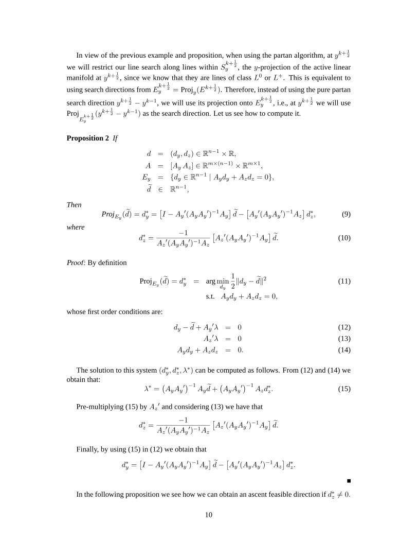
Proposition 2 If

d = (dy, dz) ∈ Rn−1 × R,

A = [Ay Az] ∈ Rm×(n−1) × Rm×1,

Ey = {dy ∈ Rn−1 | Aydy + Azdz = 0},d ∈ Rn−1,

ThenProjEy

(d) = d∗y =[I −Ay

′(AyAy′)−1Ay

]d−

[Ay

′(AyAy′)−1Az

]d∗z, (9)

where

d∗z =−1

Az′(AyAy

′)−1Az

[Az

′(AyAy′)−1Ay

]d. (10)

Proof: By definition

ProjEy(d) = d∗y = argmin

dy

12‖dy − d‖2 (11)

s.t. Aydy + Azdz = 0,

whose first order conditions are:

dy − d + Ay′λ = 0 (12)

Az′λ = 0 (13)

Aydy + Azdz = 0. (14)

The solution to this system(d∗y, d∗z, λ

∗) can be computed as follows. From (12) and (14) weobtain that:

λ∗ =(AyAy

′)−1Ayd +

(AyAy

′)−1Azd

∗z. (15)

Pre-multiplying (15) byAz′ and considering (13) we have that

d∗z =−1

Az′(AyAy

′)−1Az

[Az

′(AyAy′)−1Ay

]d.

Finally, by using (15) in (12) we obtain that

d∗y =[I −Ay

′(AyAy′)−1Ay

]d−

[Ay

′(AyAy′)−1Az

]d∗z.

In the following proposition we see how we can obtain an ascent feasible direction ifd∗z 6= 0.

10

Proposition 3 a) In the previous proposition,(d∗y, d∗z) is an ascent direction if and only ifd∗z >

0.

b) If d∗z 6= 0, then for anyγ > 0 we have thatd(γ) = (γ/d∗z)(d∗y, d

∗z) is an ascent feasible

direction.

Proof: a) For anyx we have,

∇G(x)(

d∗yd∗z

)= en

(d∗yd∗z

)= d∗z.

b) d(γ) is an ascent direction since∇G(x)d(γ) = γ > 0. It is feasible since by (14)

A d(γ) =γ

d∗z[Ay Az]

(d∗yd∗z

)=

γ

d∗z

(Ayd

∗y + Azd

∗z

)= 0.

6.1 The partan face simplex method

The above discussion is summarized in the partan face simplex method, which adapts the partanstrategy to the FS method in order to avoid the zig-zagging.

Partan face simplex method:

Step 0. Step 0. Initialization: Takex0 = (y0, z0) ∈ X such thatJ(x0) 6= ∅, ε > 0, γ > 0,K > 0, and setk = 0.

Step 1. Compute dk, the Rosen’s gradient projection as in (4).

Step 2. Compute xk+ 12 = (yk+ 1

2 , zk+ 12 ) by a global line search along Projy(d

k) as in (5).

If k = 0 then setk = k + 1 and go back to Step 1.

Step 3. Compute the Rosen’s partan projection (d∗y, d∗z):

d = yk+ 12 − yk−1,

Ak+ 12 is partitioned into[Ay Az],α = Az

′(AyAy′)−1Az.

If |α| < ε then setk = 1 and go back to Step 1,else, compute

v = Ay′(AyAy

′)−1Az,

d∗z =−1α

v′d.

If |d∗z| < ε then setk = 1 and go back to Step 1,else, compute

d∗y =[I −Ay

′(AyAy′)−1Ay

]d− d∗zv. (16)

11

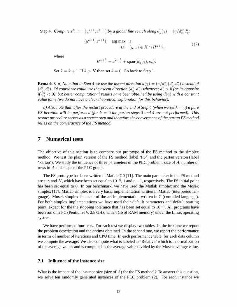
Step 4. Compute xk+1 = (yk+1, zk+1) by a global line search along dy(γ) = (γ/d∗z)d∗y:

(yk+1, zk+1) = arg max z

s.t. (y, z) ∈ X ∩Hk+ 12 ,

(17)

whereHk+ 1

2 = xk+ 12 + span{dy(γ), en}.

Setk = k + 1. If k > K then setk = 0. Go back to Step 1.

Remark 3 a) Note that in Step 4 we use the ascent directiond(γ) = (γ/d∗z)(d∗y, d

∗z) instead of

(d∗y, d∗z). Of course we could use the ascent direction(d∗y, d

∗z) wheneverd∗z > 0 (or its opposite

if d∗z < 0), but better computational results have been obtained by usingd(γ) with a constantvalue forγ (we do not have a clear theoretical explanation for this behavior).

b) Also note that, after the restart procedure at the end of Step 4 (when we setk = 0) a pureFS iteration will be performed (fork = 0 the partan steps 3 and 4 are not performed). Thisrestart procedure serves as a spacer step and therefore the convergence of the partan FS methodrelies on the convergence of the FS method.

7 Numerical tests

The objective of this section is to compare our prototype of the FS method to the simplexmethod. We test the plain version of the FS method (label ‘FS’) and the partan version (label‘Partan’). We study the influence of three parameters of the PLC problem: size ofA, number ofrows inA and shape of the PLC graph.

The FS prototype has been written in Matlab 7.0 [11]. The main parameter in the FS methodareε, γ andK, which have been set equal to10−6, 1 andn−1, respectively. The FS initial pointhas been set equal to0. In our benchmark, we have used the Matlab simplex and the Moseksimplex [17]. Matlab simplex is a very basic implementation written in Matlab (interpreted lan-guage). Mosek simplex is a state-of-the-art implementation written in C (compiled language).For both simplex implementations we have used their default parameters and default startingpoint, except for the the stopping tolerance that has been set equal to10−6. All programs havebeen run on a PC (Pentium-IV, 2.8 GHz, with 4 Gb of RAM memory) under the Linux operatingsystem.

We have performed four tests. For each test we display two tables. In the first one we reportthe problem description and the optima obtained. In the second one, we report the performancein terms of number of iterations and CPU time. In each performance table, for each data columnwe compute the average. We also compute what is labeled as ’Relative’ which is a normalizationof the average values and is computed as the average value divided by the Mosek average value.

7.1 Influence of the instance size

What is the impact of the instance size (size ofA) for the FS method ? To answer this question,we solve ten randomly generated instances of the PLC problem (2). For each instance we

12

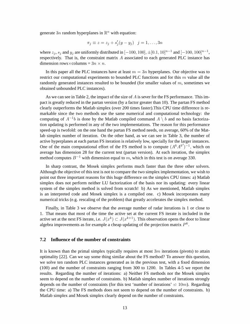
generate3n random hyperplanes inRn with equation:

πj ≡ z = zj + s′j(y − yj) j = 1, . . . , 3n

wherezj , sj andyj are uniformly distributed in[−100, 100],±[0.1, 10]n−1 and[−100, 100]n−1,respectively. That is, the constraint matrixA associated to each generated PLC instance hasdimension rows×columns =3n× n.

In this paper all the PLC instances have at leastm = 3n hyperplanes. Our objective was torestrict our computational experiments to bounded PLC functions and for thism value all therandomly generated instances resulted to be bounded (for smaller values ofm, sometimes weobtained unbounded PLC instances).

As we can see in Table 2, the impact of the size ofA is sever for the FS performance. This im-pact is greatly reduced in the partan version (by a factor greater than 10). The partan FS methodclearly outperforms the Matlab simplex (over 200 times faster).This CPU time difference is re-markable since the two methods use the same numerical and computational technology: thecomputing ofA−1b is done by the Matlab compiled commandA \ b and no basis factoriza-tion updating is performed in any of the two implementations. The reason for this performancespeed-up is twofold: on the one hand the partan FS method needs, on average, 60% of the Mat-lab simplex number of iteration. On the other hand, as we can see in Table 3, the number ofactive hyperplanes at each partan FS iteration is relatively low, specially for the larger instances.One of the main computational effort of the FS method is to compute(AkAk ′)−1, which onaverage has dimension 28 for the current test (partan version). At each iteration, the simplexmethod computesB−1 with dimension equal tom, which in this test is on average 330.

In sharp contrast, the Mosek simplex performs much faster than the three other solvers.Although the objective of this test is not to compare the two simplex implementation, we wish topoint out three important reasons for this huge difference on the simplex CPU times: a) Matlabsimplex does not perform neither LU factorization of the basis nor its updating: every linearsystem of the simplex method is solved from scratch! b) As we mentioned, Matlab simplexis an interpreted code and Mosek simplex is a compiled one. c) Mosek incorporates manynumerical tricks (e.g. rescaling of the problem) that greatly accelerates the simplex method.

Finally, in Table 3 we observe that the average number of radar iterations is 1 or close to1. That means that most of the time the active set at the current FS iterate is included in theactive set at the next FS iterate, i.e.J(xk) ⊂ J(xk+1). This observation opens the door to linearalgebra improvements as for example a cheap updating of the projection matrixP k.

7.2 Influence of the number of constraints

It is known than the primal simplex typically requires at most3m iterations (pivots) to attainoptimality [22]. Can we say some thing similar about the FS method? To answer this question,we solve ten random PLC instances generated as in the previous test, with a fixed dimension(100) and the number of constraints ranging from 300 to 1200. In Tables 4-5 we report theresults. Regarding the number of iterations: a) Neither FS methods nor the Mosek simplexseem to depend on the number of constraints. b) Matlab simplex number of iterations stronglydepends on the number of constraints (for this test ‘number of iterations’w 10m). Regardingthe CPU time: a) The FS methods does not seem to depend on the number of constraints. b)Matlab simplex and Mosek simplex clearly depend on the number of constraints.

13

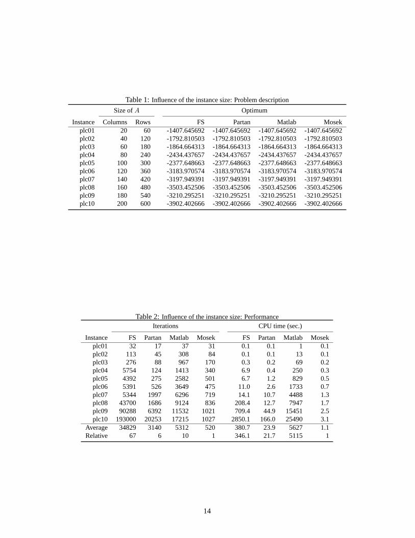
Table 1:Influence of the instance size: Problem description

Size ofA Optimum

Instance Columns Rows FS Partan Matlab Mosekplc01 20 60 -1407.645692 -1407.645692 -1407.645692 -1407.645692plc02 40 120 -1792.810503 -1792.810503 -1792.810503 -1792.810503plc03 60 180 -1864.664313 -1864.664313 -1864.664313 -1864.664313plc04 80 240 -2434.437657 -2434.437657 -2434.437657 -2434.437657plc05 100 300 -2377.648663 -2377.648663 -2377.648663 -2377.648663plc06 120 360 -3183.970574 -3183.970574 -3183.970574 -3183.970574plc07 140 420 -3197.949391 -3197.949391 -3197.949391 -3197.949391plc08 160 480 -3503.452506 -3503.452506 -3503.452506 -3503.452506plc09 180 540 -3210.295251 -3210.295251 -3210.295251 -3210.295251plc10 200 600 -3902.402666 -3902.402666 -3902.402666 -3902.402666

Table 2:Influence of the instance size: PerformanceIterations CPU time (sec.)

Instance FS Partan Matlab Mosek FS Partan Matlab Mosekplc01 32 17 37 31 0.1 0.1 1 0.1plc02 113 45 308 84 0.1 0.1 13 0.1plc03 276 88 967 170 0.3 0.2 69 0.2plc04 5754 124 1413 340 6.9 0.4 250 0.3plc05 4392 275 2582 501 6.7 1.2 829 0.5plc06 5391 526 3649 475 11.0 2.6 1733 0.7plc07 5344 1997 6296 719 14.1 10.7 4488 1.3plc08 43700 1686 9124 836 208.4 12.7 7947 1.7plc09 90288 6392 11532 1021 709.4 44.9 15451 2.5plc10 193000 20253 17215 1027 2850.1 166.0 25490 3.1

Average 34829 3140 5312 520 380.7 23.9 5627 1.1Relative 67 6 10 1 346.1 21.7 5115 1

14

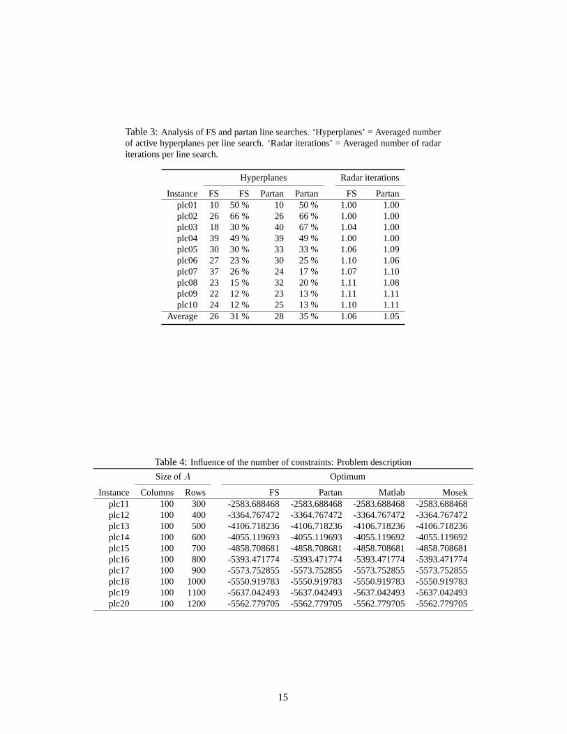
Table 3:Analysis of FS and partan line searches. ‘Hyperplanes’ = Averaged numberof active hyperplanes per line search. ‘Radar iterations’ = Averaged number of radariterations per line search.

Hyperplanes Radar iterations

Instance FS FS Partan Partan FS Partanplc01 10 50 % 10 50 % 1.00 1.00plc02 26 66 % 26 66 % 1.00 1.00plc03 18 30 % 40 67 % 1.04 1.00plc04 39 49 % 39 49 % 1.00 1.00plc05 30 30 % 33 33 % 1.06 1.09plc06 27 23 % 30 25 % 1.10 1.06plc07 37 26 % 24 17 % 1.07 1.10plc08 23 15 % 32 20 % 1.11 1.08plc09 22 12 % 23 13 % 1.11 1.11plc10 24 12 % 25 13 % 1.10 1.11

Average 26 31 % 28 35 % 1.06 1.05

Table 4:Influence of the number of constraints: Problem description

Size ofA Optimum

Instance Columns Rows FS Partan Matlab Mosekplc11 100 300 -2583.688468 -2583.688468 -2583.688468 -2583.688468plc12 100 400 -3364.767472 -3364.767472 -3364.767472 -3364.767472plc13 100 500 -4106.718236 -4106.718236 -4106.718236 -4106.718236plc14 100 600 -4055.119693 -4055.119693 -4055.119692 -4055.119692plc15 100 700 -4858.708681 -4858.708681 -4858.708681 -4858.708681plc16 100 800 -5393.471774 -5393.471774 -5393.471774 -5393.471774plc17 100 900 -5573.752855 -5573.752855 -5573.752855 -5573.752855plc18 100 1000 -5550.919783 -5550.919783 -5550.919783 -5550.919783plc19 100 1100 -5637.042493 -5637.042493 -5637.042493 -5637.042493plc20 100 1200 -5562.779705 -5562.779705 -5562.779705 -5562.779705

15

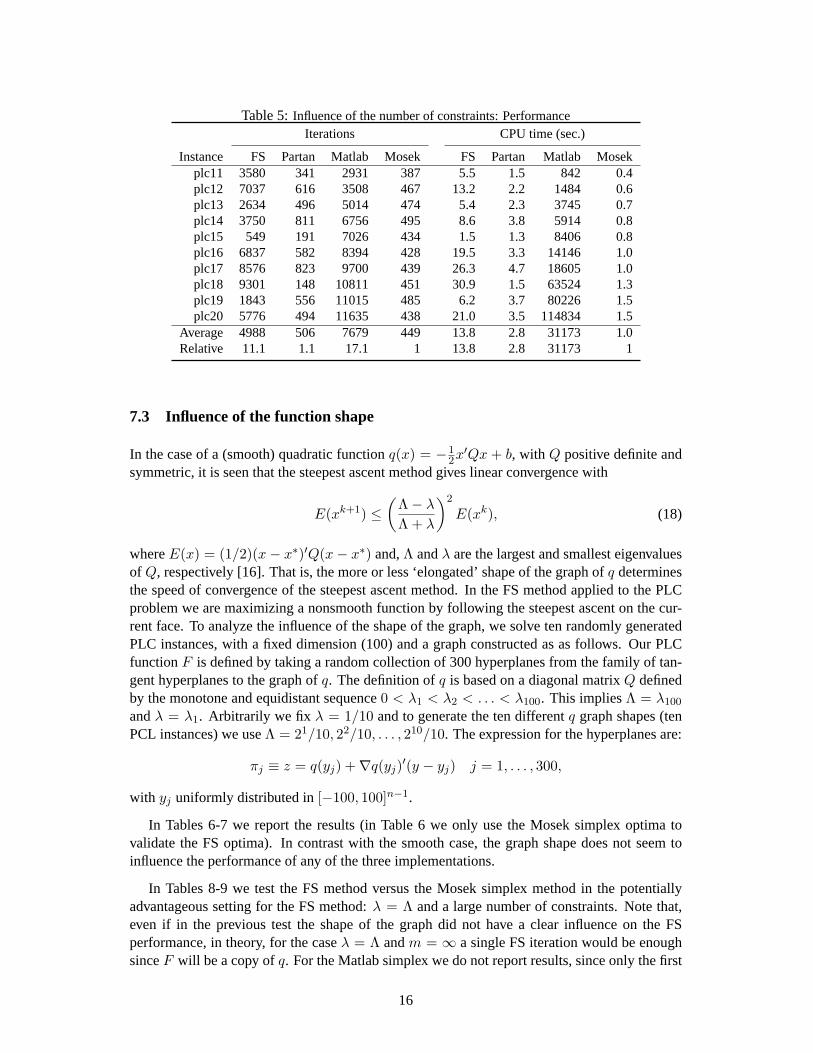
Table 5:Influence of the number of constraints: PerformanceIterations CPU time (sec.)

Instance FS Partan Matlab Mosek FS Partan Matlab Mosekplc11 3580 341 2931 387 5.5 1.5 842 0.4plc12 7037 616 3508 467 13.2 2.2 1484 0.6plc13 2634 496 5014 474 5.4 2.3 3745 0.7plc14 3750 811 6756 495 8.6 3.8 5914 0.8plc15 549 191 7026 434 1.5 1.3 8406 0.8plc16 6837 582 8394 428 19.5 3.3 14146 1.0plc17 8576 823 9700 439 26.3 4.7 18605 1.0plc18 9301 148 10811 451 30.9 1.5 63524 1.3plc19 1843 556 11015 485 6.2 3.7 80226 1.5plc20 5776 494 11635 438 21.0 3.5 114834 1.5

Average 4988 506 7679 449 13.8 2.8 31173 1.0Relative 11.1 1.1 17.1 1 13.8 2.8 31173 1

7.3 Influence of the function shape

In the case of a (smooth) quadratic functionq(x) = −12x′Qx + b, with Q positive definite and

symmetric, it is seen that the steepest ascent method gives linear convergence with

E(xk+1) ≤(

Λ− λ

Λ + λ

)2

E(xk), (18)

whereE(x) = (1/2)(x− x∗)′Q(x− x∗) and,Λ andλ are the largest and smallest eigenvaluesof Q, respectively [16]. That is, the more or less ‘elongated’ shape of the graph ofq determinesthe speed of convergence of the steepest ascent method. In the FS method applied to the PLCproblem we are maximizing a nonsmooth function by following the steepest ascent on the cur-rent face. To analyze the influence of the shape of the graph, we solve ten randomly generatedPLC instances, with a fixed dimension (100) and a graph constructed as as follows. Our PLCfunctionF is defined by taking a random collection of 300 hyperplanes from the family of tan-gent hyperplanes to the graph ofq. The definition ofq is based on a diagonal matrixQ definedby the monotone and equidistant sequence0 < λ1 < λ2 < . . . < λ100. This impliesΛ = λ100

andλ = λ1. Arbitrarily we fix λ = 1/10 and to generate the ten differentq graph shapes (tenPCL instances) we useΛ = 21/10, 22/10, . . . , 210/10. The expression for the hyperplanes are:

πj ≡ z = q(yj) +∇q(yj)′(y − yj) j = 1, . . . , 300,

with yj uniformly distributed in[−100, 100]n−1.

In Tables 6-7 we report the results (in Table 6 we only use the Mosek simplex optima tovalidate the FS optima). In contrast with the smooth case, the graph shape does not seem toinfluence the performance of any of the three implementations.

In Tables 8-9 we test the FS method versus the Mosek simplex method in the potentiallyadvantageous setting for the FS method:λ = Λ and a large number of constraints. Note that,even if in the previous test the shape of the graph did not have a clear influence on the FSperformance, in theory, for the caseλ = Λ andm = ∞ a single FS iteration would be enoughsinceF will be a copy ofq. For the Matlab simplex we do not report results, since only the first

16

Table 6: Influence of the function shape: Problem description. All instances are ofsize rows×columns = 300×100.

Maximum Optimum

Instance Eigenvalue FS Partan Mosekplc21 2/10 2.2956216726×104 2.2956216726×104 2.2956216726×104

plc22 4/10 3.7530005959×104 3.7530005959×104 3.7530005959×104

plc23 8/10 6.7130365536×104 6.7130365536×104 6.7130365536×104

plc24 16/10 1.2959614351×105 1.2959614351×105 1.2959614351×105

plc25 32/10 2.4991985084×105 2.4991985084×105 2.4991985084×105

plc26 64/10 4.9278816291×105 4.9278816291×105 4.9278816291×105

plc27 128/10 9.6795507723×105 9.6795507723×105 9.6795507723×105

plc28 256/10 1.9246016667×106 1.9246016667×106 1.9246016667×106

plc29 512/10 3.8775769072×106 3.8775769072×106 3.8775769073×106

plc30 1024/10 7.7649034444×106 7.7649034444×106 7.7649034449×106

Table 7:Influence of the function shape: Performance

Iterations CPU time (sec.)

Instance FS Partan Matlab Mosek FS Partan Matlab Mosekplc21 4776 1064 3829 483 7.0 3.6 360 0.5plc22 1978 306 3511 380 2.9 1.3 319 0.5plc23 443 126 4348 410 1.1 0.8 418 0.5plc24 970 386 4330 523 1.7 1.8 408 0.5plc25 1701 158 3938 395 2.7 1.3 330 0.4plc26 1569 382 4102 444 2.7 2.6 344 0.5plc27 2199 489 3594 441 3.6 3.6 278 0.5plc28 2212 1045 3579 474 3.7 5.7 291 0.6plc29 30007 784 3508 332 79.3 4.5 273 0.6plc30 1020 1971 4707 399 1.9 9.2 401 0.4

Average 4688 671 3945 428 10.7 3.4 342 0.5Relative 11.0 1.6 9.2 1 21.4 6.8 684 1

two instances were solved in less than105 seconds. For the Mosek simplex method we giveresults for the PLC problem (3) and for its equivalent dual formulation (DF):

miny∈Rm

{b′y | A′y = en, y ≥ 0}.

Again, we encounter an important difference between the smooth and non smooth case. Fora (smooth) quadratic function, by (18), the steepest ascent method will need one single iterationwheneverλ = Λ. In Tables 9 we observe that many FS iterations may me needed even if the(nonsmooth) PLC function has been derived from a quadratic function withλ = Λ).

For this particular class of PLC instances we can say that the partan FS method outperformsthe simplex method since the CPU times are similar and the FS prototype is coded in Matlab.Of course, when using the simplex method, in the case of a large number of constraints a betterchoice is to solve the dual formulation.

17

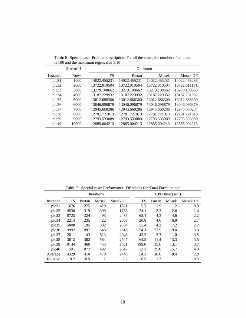
Table 8:Special case: Problem description. For all the cases, the number of columnsis 100 and the maximum eigenvalue 1/10

Size ofA Optimum

Instance Rows FS Partan Mosek Mosek DFplc31 1000 14022.455231 14022.455231 14022.455231 14022.455235plc32 2000 13722.010504 13722.010504 13722.010504 13722.011171plc33 3000 13279.100662 13279.100662 13279.100662 13279.100663plc34 4000 13187.229932 13187.229932 13187.229932 13187.231032plc35 5000 13012.686300 13012.686300 13012.686300 13012.686300plc36 6000 13046.096879 13046.096879 13046.096879 13046.096879plc37 7000 12945.660286 12945.660286 12945.660286 12945.660287plc38 8000 12781.721013 12781.721013 12781.721013 12781.721013plc39 9000 12793.533089 12793.533089 12793.533089 12793.533089plc40 10000 12885.004213 12885.004213 12885.004213 12885.004213

Table 9:Special case: Performance. DF stands for ‘Dual Formulation’

Iterations CPU time (sec.)

Instance FS Partan Mosek Mosek DF FS Partan Mosek Mosek DFplc31 1676 275 420 1821 5.3 1.9 1.2 0.9plc32 4530 319 399 1788 24.1 3.3 2.6 1.4plc33 8723 324 493 2485 63.4 4.3 4.6 2.2plc34 2214 235 422 2803 20.8 4.0 6.0 2.7plc35 5000 195 382 2304 55.4 4.2 7.2 2.7plc36 3992 897 543 2518 54.1 21.9 9.4 3.0plc37 2811 143 513 2948 43.2 3.7 11.0 3.5plc38 3612 382 584 2547 64.8 11.4 13.3 3.5plc39 10144 460 453 2621 199.0 15.6 13.1 3.7plc40 591 872 492 2647 13.2 35.0 15.7 4.0

Average 4329 410 470 2448 54.3 10.6 8.4 2.8Relative 9.2 0.9 1 5.2 6.5 1.3 1 0.3

18

8 Conclusions

In the framework of the Kelley cutting plane method, the face simplex (FS) method is an alter-native to the simplex method to maximize a piecewise linear concave (PLC) function. It is wellknown that the simplex method at the current vertex takes an ascending edge and stops at theother vertex of the edge. In this paper we address the question of what would happen if insteadof stopping the line search at the second vertex, one continues the line search on the whole PLCsurface up to the best point? The FS method gives a plausible answer.The FS method freelyexplores the polyhedral surface by following the Rosen’s gradient projection combined with aglobal line search on the whole surface.

From a theoretical point of view, we have therefore enlarged the Rosen’s gradient projectionsteps by using the radar method to perform a global line search. The other theoretical contribu-tion has been to adapt the partan method, a conjugate gradient technique, to the case of a PLCfunction (partan face simplex method). Roughly speaking, this partan version has reduced thenumber of the plain FS iterations by a factor of 10, by avoiding zig-zagging. The CPU time im-proved by a factor of 5 since each partan FS iteration amounts to two plain FS iterations in termsof computational work. Finally, although we have proved the convergence of the FS method fordimension 3, convergence for the general case remains an open question.

From a computational point of view, we have compared the FS Matlab prototypes to tworepresentative implementations of the simplex method. Matlab simplex, a very basic interpretedimplementation and Mosek simplex, a state-of-the-art compiled implementation. Comparedto Matlab simplex, the performance of the partan FS prototype is very competitive, mainlydue to two reasons: Matlab simplex does not use any LU basis factorization/updating. On theother hand, in the FS method the computational effort is low since only a small fraction of theconstraints is considered at each iteration. Compared to the Mosek simplex method, the partanFS prototype does not seem competitive except for the case of a large number of constraints.However, we think that in the FS method there is still room for numerical improvements.

Even if the FS method does not seem to outperform the simplex method, it has two inherentadvantages compared to the simplex method: First, the FS method does not need the expensiveinitialization of the simplex method (to find an initial vertex). Second, in the case of a PLCunconstrained function, it may happen that an optimal vertex does not exist. In contrast with theFS method, the simplex method simply will not be able to optimize such a function or will needto bound the variables in an artificial way, if it made sense to do it.

Acknowledgment

The author is thankful to Jean-Philippe Vial, Alain Haurie and Nidhi Sawhney for theircomments and support at Logilab, HEC, University of Geneva.

References

[1] F. Baboneau, C. Beltran, A. B. Haurie, C. Tadonki, and J.-Ph. Vial. Proximal-accpm: aversatile oracle based optimization method. In‘Advances in Computational Economics,Finance and Management Science’, to appear in ‘Computational Management Science’.Kluwer.

19

[2] C. Beltran and F. J. Heredia. An effective line search for the subgradient method.Journalon Optimization Theory and Applications, 125(1):1–18, 2005.

[3] C. Beltran-Royo. Line search for piecewise linear functions by the radar method. Technicalreport, Logilab, HEC, University of Geneva, 2005.

[4] Dimitri. P. Bertsekas.Nonlinear Programming. Ed. Athena Scientific, Belmont, Mas-sachusetts, (USA), 2n edition, 1999.

[5] G. W. Brown and T. C. Koopmans. Computational suggestions for maximizing a linearfunction subject to linear inequalities. In T. C. Koopmans, editor,Activity Analysis ofProduction and Allocation, pages 377–380, New York, 1951. Wiley.

[6] S. Y. Chang and K. G. Murty. The steepest descent gravitational method for linear pro-gramming.Discrete Applied Mathematics, 25:211–239, 1989.

[7] A. R. Conn and G. Cornuejols. A projection method for the uncapacitated facility locationproblem.Mathematical programming, 46:373–398, 1990.

[8] Sherali H. D. and I. Al-loughani. Solving euclidean distance multifacility location prob-lems using conjugate subgradients and line-search methods.Computational optimizationand applications, 14:275–291, 1999.

[9] D.-Z. Du and X.-S. Zhang. Global convergence of rosen’s gradient projection method.Mathematical Programming, 44(3):357–366, 1989.

[10] W. W. Hager and S. Park. The gradient projection method with exact line search.Journalof Global Optimization, 30(1):103–118, 2004.

[11] D. J. Higham and N. J. Higham.MATLAB guide. SIAM, Philadelphia, Pennsilvania, USA,2000.

[12] J. B. Hiriart-Urruty and C. Lemarechal. Convex Analysis and Minimization Algorithms,volume I and II. Springer-Verlag, Berlin, 1996.

[13] J.-B. Hiriart-Urruty and C. Lemarechal.Fundamentals of convex analysis. Springer, 2000.

[14] J. E. Kelley. The cutting-plane method for solving convex programs.Journal of the SIAM,8:703–712, 1960.

[15] C. Lemke. The constrained gradient method of linear programming.SIAM, 9(1):1–17,1961.

[16] D. G. Luenberger.Linear and Nonlinear Programming. Addison-Wesley, Reading, Mas-sachusetts, USA, second edition, 1984.

[17] ApS Mosek. Version 3.1.1.42, copyright (c), 1998-2004. http://www.mosek.com.

[18] P. Neame, N. Boland, and D. Ralph. An outer approximate subdifferential method forpiecewise affine optimization.Mathematical programming, Ser. A 87:57–86, 2000.

[19] J. Rosen. The gradient projection method for nonlinear programming, I. linear constraints.Journal of the Society for Industrial and Applied Mathematics, 8:181–217, 1960.

20

[20] B. Shah, R. Buehler, and O. Kempthorne. Some algorithms for minimizing a function ofseveral variables.Journal of the Society for Industrial and Applied Mathematics, 12(1):74–92, 1964.

[21] N. Z. Shor. Nondifferentiable optimization and polynomial problems. Nonconvex opti-mization and its applications. Kluwer academic publishers, 1998.

[22] M. J. Todd. The many facets of linear programming.Mathematical Programming, Ser. B91:417–436, 2002.

[23] P. Wolfe. A method of conjugate subgradients for minimizing nondifferentiable functions.Mathematical Programming Study, 3:145–173, 1975.

[24] X.-S. Zhang. On the convergence of rosen’s gradient projection method: Three-dimensional case (in chinese).Acta Mathematicae Applicatae Sinica, 8, 1985.

[25] G Zoutendijk.Methods of feasible directions. Elsevier, Amsterdan, 1960.

21