BORDERS, GEOGRAPHY, AND OLIGOPOLY:...

BORDERS, GEOGRAPHY, AND OLIGOPOLY: EVIDENCE FROM THE WINDTURBINE INDUSTRY

A. Kerem Cosar, Paul L. E. Grieco, and Felix Tintelnot*

Abstract—Using a microlevel data set of wind turbine installations inDenmark and Germany, we estimate a structural oligopoly model withcross-border trade and heterogeneous firms. Our approach separately iden-tifies border-related from distance-related variable costs and bounds thefixed cost of exporting for each firm. In the data, firms’ market shares dropprecipitously at the border. We find that 40% to 50% of the gap can beattributed to national border costs. Counterfactual analysis indicates thateliminating national border frictions would increase total welfare in thewind turbine industry by 4% in Denmark and 6% in Germany.

I. Introduction

DISTANCE and political borders lead to geographic andnational segmentation of markets. In turn, the size and

structure of markets depend crucially on the size and nature oftrade costs. A clear understanding of these costs is thus impor-tant for assessing the impact of many government policies.1Since the seminal work of McCallum (1995), an extensiveliterature has documented significant costs related to cross-ing national boundaries. Estimated magnitudes of borderfrictions are so large that some researchers have suggestedthey are due to spatial and industry-level aggregation bias, afailure to account for within-country heterogeneity and geog-raphy, and cross-border differences in market structure.2 Toavoid these potentially confounding effects, we use spatialmicrodata from wind turbine installations in Denmark andGermany to estimate a structural model of oligopolistic com-petition with border frictions. Our main findings are that (a)border frictions are large within the wind turbine industry,(b) fixed and variable costs of exporting are both importantin explaining overall border frictions, and (c) these frictionshave a substantial impact on welfare.

Our ability to infer various components of trade costs isa result of our focus on a narrowly defined industry: wind

Received for publication April 16, 2013. Revision accepted forpublication May 19, 2014. Editor: Gordon Hanson.

* Cosar: University of Chicago; Grieco: Pennsylvania State University;Tintelnot: University of Chicago and Princeton University.

For their insightful comments and constructive suggestions, we thankCostas Arkolakis, Lorenzo Caliendo, Allan Collard-Wexler, Steve Davis,Jonathan Eaton, Charles Engel, Oleg Itskhoki, Samuel Kortum, KalaKrishna, Jan De Loecker, Matthias Lux, Ferdinando Monte, EduardoMorales, Brent Neiman, Dennis Novy, Ralph Ossa, Ayse Pehlivan, JorisPinkse, Mark Roberts, Andrés Rodríguez-Clare, Alan Spearot, Elie Tamer,Jonathan Vogel, Stephen Yeaple, Nicholas Ziebarth, the editor, two anony-mous referees, and numerous seminar participants. For their valuablediscussions with us about the industry, we thank Wolfgang Conrad, RobertJuettner, Alex Kaulen, and Jochen Twele.

A supplemental appendix is available online at http://www.mitpressjournals.org/doi/suppl/10.1162/REST_a_00485.

1 Policy relevance goes beyond trade policies. According to Obstfeld andRogoff (2001), core empirical puzzles in international macroeconomics canbe explained as a result of costs in the trade of goods. The effectiveness ofdomestic regulation in some industries may hinge on the extent of tradeexposure, as shown by Fowlie, Reguant, and Ryan (2012) for the U.S.Portland cement industry.

2 See Hillberry (2002), Hillberry and Hummels (2008), Broda andWeinstein (2008), and Gorodnichenko and Tesar (2009).

turbine manufacturing. In addition to being an interestingcase for study in its own right due to the growing importanceof wind energy to the energy portfolios of many coun-tries, the wind turbine industry in the European Union (EU)offers an excellent opportunity to examine the effects ofnational boundaries on market segmentation. First, we haverich spatial information on the location of manufacturers andinstallations. The data are much finer than previously usedaggregate state- or province-level data. The use of disaggre-gated data allows us to account for actual shipping distancesrather than rely on market-to-market distances, to estimateborder costs. Second, the data contain observations of bothdomestic and international trade. We observe active manufac-turers on either side of the Danish-German border, some ofwhom choose to export and some of whom do not, allowingus to separate fixed and variable border costs. Third, intra-EU trade is free from formal barriers and large exchange ratefluctuations. National subsidies are directed only toward thegeneration of renewable electricity. By the Single EuropeanAct, they do not discriminate against other European produc-ers of turbines. The border costs in this setting are thereforedue to factors other than formal barriers to trade.

Despite substantial formal integration, the data indicatesignificant market segmentation between Denmark and Ger-many. Examining the sales of turbines in 1995 and 1996, wefind that domestic manufacturers have a substantially highermarket share than foreign manufacturers. For example, thetop five German manufacturers possess a market share of60% in Germany and only 2% in Denmark. There appearto be border frictions on both the extensive and intensivemargins: in the extensive margin, only one of the five largeGerman firms exports to Denmark. In contrast, all five largeDanish firms have sales in Germany. In the intensive mar-gin, however, their market share is substantially lower in theforeign market and drops discontinuously at the border.

We propose a model to explain these patterns and study thewelfare implications of the border. Firms are heterogeneousin their qualities, costs, and primary manufacturing location.The model has two stages. In the first stage, turbine producersdecide whether to export. Exporting firms must pay a fixedentry cost specific to them. In the second stage, turbine pro-ducers observe the set of active producers in each marketand engage in price competition for each project. This givesrise to a spatial model of demand for wind turbine instal-lations. From the sourcing decision of project managers, wecan identify internal and international variable border costs byexploiting variation across firms and projects in their distanceto federal and national borders. Since borders are responsiblefor a discrete jump in costs, they can be separated from thesteady increase in costs related to distance. The model thusdelivers endogenous variation in prices, markups, and market

The Review of Economics and Statistics, July 2015, 97(3): 623–637© 2015 by the President and Fellows of Harvard College and the Massachusetts Institute of Technologydoi:10.1162/REST_a_00485

624 THE REVIEW OF ECONOMICS AND STATISTICS

shares across points in space, so we are able to analyze theimpact of the border on trade flows, as well as producer andconsumer surplus.

Our results indicate substantial variable and fixed coststo sell wind turbines across the border between Denmarkand Germany.3 Whereas German firms face nonnegligiblevariable costs when competing outside their home state, thevariable border costs associated with the national borderare roughly 85% higher. While fixed foreign market entrycosts are not point identified by our model, we are able togauge their significance through counterfactual analysis. Weconduct two counterfactual experiments in which we firsteliminate fixed entry costs and then all international borderfrictions. Market segmentation declines as we remove fric-tions to both the extensive and intensive margins. Overall,we find that the elimination of international border frictionsraises consumer surplus by 8.6% and 8.8% in Denmark andGermany, respectively. Total surplus increases by 4.3% inDenmark and 5.6% in Germany.

By estimating a structural oligopoly model that controls forinternal geography and firm heterogeneity, this paper adds tothe empirical literature on trade costs. Early contributions byMcCallum (1995) and Anderson and van Wincoop (2003)use data on interstate, interprovincial, and international tradeflows between Canada and the United States to document adisproportionately high level of intranational trade betweenCanadian provinces and U.S. states after controlling forincome levels of regions and the distances between them.Alternatively, Engel and Rogers (1996), Gopinath et al.(2011), and Goldberg and Verboven (2001, 2005) have doc-umented market segmentation by studying internal versuscross-border price dispersion.

Rather than inferring a “border effect” or “width of the bor-der” based on differences between intra- and internationaltrade flows or price differentials, we estimate a structuralmodel of market segmentation using spatial microdata. Bydoing so, we address several critiques raised by the literature.Hillberry (2002), Hillberry and Hummels (2008), and Brodaand Weinstein (2008) have argued that sectoral, geographic,and product-level aggregation may lead to upward bias in theestimation of the border effect in studies that use trade flows.Holmes and Stevens (2012) emphasize the importance ofcontrolling for internal distances. Our study addresses thesecritiques since our data enable us to precisely calculate thedistances between consumption and production locations fora narrowly defined product. That in turn enables us to sepa-rate the impact of distance from the impact of the border. Inaddition, we can use our model to quantify the producer andconsumer surplus implications of cross-border trade barriers.

3 We assume that all border frictions are related to costs rather than homebias on the part of project managers. In consumer goods industries, pref-erences may discontinuously change at the border if consumers act on ahome bias toward domestic producers. In our setting, where consumers areprofit maximizers purchasing an investment good, we expect that demand-driven home bias is small. Alternatively, we can interpret our cost estimatesas incorporating the additional costs that exporting firms must incur toovercome any home bias in preferences.

In summary, our industry-specific focus has three majoradvantages: First, the use of precise data on locations in astructural model allows for a clean identification of costsrelated to distance and border. Second, the model controls forendogenous variation in markups across markets within andacross countries based on changes in the competitive struc-ture across space. Third, by distinguishing between fixed andvariable border costs, we gain a deeper insight into the sourcesof border frictions than we do from studies that use aggregatedata.

II. Industry Background and Data

Encouraged by generous subsidies for wind energy, Ger-many and Denmark have been at the forefront of what hasbecome a worldwide boom in the construction of wind tur-bines. Large-scale production and installation of electricitygenerating wind-turbines became popular after the introduc-tion of feed-in-tariff subsidies for wind energy generation in1984 in Denmark and in 1991 in Germany. Owners of windfarms are paid for the electricity they produce and provideto the electric grid. In both countries, national governmentsregulate the unit price paid by grid operators to site owners.These “feed-in-tariffs” are substantially higher than the mar-ket rate for other electricity sources. Important for our studyis that remuneration for renewable energy is not conditionalon purchasing turbines from domestic turbine manufactur-ers, which would be in violation of European single-marketpolicy. Therefore, it is in the best interest of the wind farmowner to purchase the turbine that maximizes his or her profitsindependent of the nationality of the manufacturer.

The project manager’s choice of manufacturer is our pri-mary focus. In the period we study, purchasers of windturbines were primarily small independent investors.4 Theturbine manufacturing industry, however, is dominated by asmall number of firms that manufacture, construct, and main-tain turbines on the project owner’s land. Manufacturers usu-ally have a portfolio of turbine designs available with variousgenerating capacities. Overall, their portfolios are relativelyhomogeneous in terms of observable characteristics.5

The proximity of the production location to the projectsite is an important driver of cost differences across projects.Due to the size and weight of turbine components, oversizedcargo shipments typically necessitate road closures along the

4 Small purchasers were encouraged by financial incentive schemes thatgave larger remuneration to small producers such as cooperative invest-ment groups and private owners. The German Electricity Feed Law of1991 explicitly ruled out price support for installations in which the FederalRepublic of Germany, a federal state, a public electricity utility, or one ofits subsidiaries held shares of more than 25%. The Danish support schemeprovided about 30% higher financial compensation for independent produc-ers of renewable electricity (Sijm, 2002). A new law passed in Germany in2000 eliminated the restrictions for public electricity companies to benefitfrom above-market pricing of renewable energy.

5 Main observable product characteristics are generation capacity, towerheight, and rotor diameter. Distribution of turbines in terms of these vari-ables is very similar in both countries. Further details are displayed inappendix B in the online appendix.

BORDERS, GEOGRAPHY, AND OLIGOPOLY 625

delivery route. According to industry sources, transportationcosts range between 6% and 20% of total costs (Franken &Weber, 2008). Plant-to-project distances also affect the costof postsale services (such as maintenance), installing remotecontrollers to monitor wind farm operations, gathering infor-mation about sites farther away from the manufacturer’slocation, and maintaining relationships with local contractorswho construct turbine towers.6

Intra- and international political boundaries impose othervariable costs on firms. Industry experts highlight severalsources of friction. In the case of state borders, these costs arerelated to administrative hurdles in coordinating transporta-tion across different agencies, acquiring building permits,and interacting with regional operators to connect projectsto the grid. The banking sector, which is critical for obtain-ing project financing, is also typically organized at the stateor local level. Moreover, firms that are local employers ben-efit from greater visibility than their out-of-state competitorsdo. In addition to the cost of selling across an intranationalborder, the international border imposes even higher transac-tion costs. Additional channels include the cost of writing andenforcing international contracts and dealing with a differentcurrency, language, and culture.

In contrast to distance and variable border costs, fixed mar-ket entry costs are incurred only on entering a foreign market.Differences in the electricity grid in Denmark and Germanyrequire the development and installation of a country-specificsoftware that regulates generation. Similarly, each turbinemodel undergoes a separate certification process in eachcountry before it can be marketed. In order to overcomedifferences in language and business practices, firms mayestablish country-specific sales teams. These fixed entry costsmay prevent a firm from competing for projects in the foreignmarket at all. Accounting for these costs will be important,as they may substantially change the market structure (i.e.,the number of competitors) on either side of the border.

A. Data

We have collected data on every installation of a windturbine in Denmark and Germany dating to the birth of thewind turbine industry. The data include the location of eachproject, the number of turbines, the total megawatt capac-ity, the date of grid connection, manufacturer identity, andother turbine characteristics, such as rotor diameter and towerheights. Using the location of each manufacturer’s primaryproduction facility, we calculate road distances from eachmanufacturer to each project. This provides us with a spatial

6 For a rough comparison of the effect that distance has in this indus-try against common benchmarks in the literature, appendix A estimates agravity equation on international trade in the six-digit HS 2007 product cat-egory associated with wind turbines. The results indicate that the industry isremarkably representative in terms of distance and contiguity. We take thisas evidence that while distance is an important driver of costs in the industry,its effect is not inordinately large relative to other tradable manufacturedgoods.

source of variation in manufacturer costs that aids in identi-fying the sources of market segmentation. While our data arerich in the spatial dimension, we do not observe transactionprices due to the business-to-business nature of the industry.(Appendix B provides a detailed description of the data.)

In this paper, we concentrate on the years 1995 to 1996.This has several advantages. First, the set of firms was stableduring this time period. There are several medium-to-largefirms competing in the market. In 1997, a merger and acquisi-tion wave began, which lasted until 2005. This wave includesa cross-border acquisition, which would blur the distinctionbetween a foreign and domestic firm and complicate our anal-ysis of the border effect.7 Second, site owners in this periodwere typically independent producers. This contrasts withlater periods when utility companies became significant pur-chasers of wind turbines, leading to more concerns aboutrepeated interaction between purchasers and manufacturers.Third, this period contains several well-established firms, andthe national price subsidies for wind electricity generationhad been in place for several years. Prior to the mid-1990s, themarket could be considered an infant industry with substantialuncertainty about the viability of firms and downstream sub-sidies. Fourth, starting in the late 1990s, a substantial fractionof wind turbine installations are offshore, so road distance tothe turbine location is no longer a useful source of variationin production costs.

In focusing on a two-year period, we abstract away fromsome dynamic considerations. Although this greatly sim-plifies the analysis, it comes with some drawbacks. Mostimportant is that one cannot distinguish sunk costs fromfixed costs of entering the foreign export market (Roberts& Tybout, 1997; Das, Roberts, & Tybout, 2007). Because ofthe small number of firms and the lack of substantial entry andexit, it would not be possible to reliably estimate sunk costsand fixed costs separately in any case. We must also abstractaway from the possibility of collusion that could result fromrepeated interaction (Salvo, 2010), although we have no rea-son to expect that collusion occurred in this industry. Instead,we model the decision to enter a foreign market as a one-shotgame. This decision does not affect the consistency of ourvariable cost estimates, whereas our counterfactuals remov-ing fixed costs should be interpreted as removing both sunkand fixed costs.

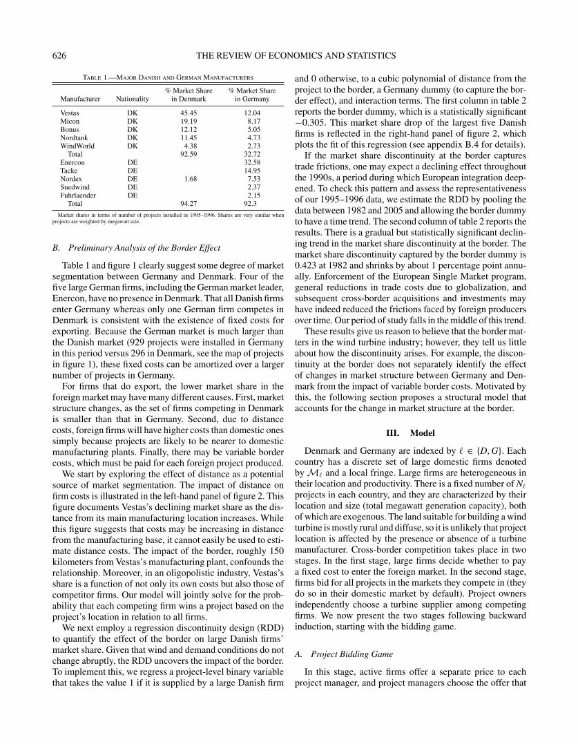
Table 1 displays the market shares of the largest five Danishand German firms in both countries. We take these firms tobe the set of manufacturers in our study. In the left panelof figure 1, we present the project locations using separatemarkers for German and Danish produced projects. The rightpanel provides the location of the primary production facilityfor each turbine manufacturer.

7 On the other hand, the specter of a merger wave presents the possibilityof anticipatory effects. For example, if a firm was seen as a likely mergertarget, this might affect its reputation given that servicing a turbine in thefuture is typically the responsibility of the manufacturing firm. We controlfor these effects through firm fixed effects to allow the reputation of firmsto be heterogeneous.


Table 1.—Major Danish and German Manufacturers

% Market Share % Market ShareManufacturer Nationality in Denmark in Germany

Vestas DK 45.45 12.04Micon DK 19.19 8.17Bonus DK 12.12 5.05Nordtank DK 11.45 4.73WindWorld DK 4.38 2.73

Total 92.59 32.72Enercon DE 32.58Tacke DE 14.95Nordex DE 1.68 7.53Suedwind DE 2.37Fuhrlaender DE 2.15

Total 94.27 92.3

Market shares in terms of number of projects installed in 1995–1996. Shares are very similar whenprojects are weighted by megawatt size.

B. Preliminary Analysis of the Border Effect

Table 1 and figure 1 clearly suggest some degree of marketsegmentation between Germany and Denmark. Four of thefive large German firms, including the German market leader,Enercon, have no presence in Denmark. That all Danish firmsenter Germany whereas only one German firm competes inDenmark is consistent with the existence of fixed costs forexporting. Because the German market is much larger thanthe Danish market (929 projects were installed in Germanyin this period versus 296 in Denmark, see the map of projectsin figure 1), these fixed costs can be amortized over a largernumber of projects in Germany.

For firms that do export, the lower market share in theforeign market may have many different causes. First, marketstructure changes, as the set of firms competing in Denmarkis smaller than that in Germany. Second, due to distancecosts, foreign firms will have higher costs than domestic onessimply because projects are likely to be nearer to domesticmanufacturing plants. Finally, there may be variable bordercosts, which must be paid for each foreign project produced.

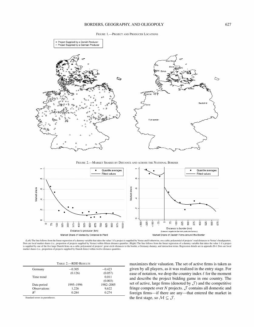
We start by exploring the effect of distance as a potentialsource of market segmentation. The impact of distance onfirm costs is illustrated in the left-hand panel of figure 2. Thisfigure documents Vestas’s declining market share as the dis-tance from its main manufacturing location increases. Whilethis figure suggests that costs may be increasing in distancefrom the manufacturing base, it cannot easily be used to esti-mate distance costs. The impact of the border, roughly 150kilometers from Vestas’s manufacturing plant, confounds therelationship. Moreover, in an oligopolistic industry, Vestas’sshare is a function of not only its own costs but also those ofcompetitor firms. Our model will jointly solve for the prob-ability that each competing firm wins a project based on theproject’s location in relation to all firms.

We next employ a regression discontinuity design (RDD)to quantify the effect of the border on large Danish firms’market share. Given that wind and demand conditions do notchange abruptly, the RDD uncovers the impact of the border.To implement this, we regress a project-level binary variablethat takes the value 1 if it is supplied by a large Danish firm

and 0 otherwise, to a cubic polynomial of distance from theproject to the border, a Germany dummy (to capture the bor-der effect), and interaction terms. The first column in table 2reports the border dummy, which is a statistically significant−0.305. This market share drop of the largest five Danishfirms is reflected in the right-hand panel of figure 2, whichplots the fit of this regression (see appendix B.4 for details).

If the market share discontinuity at the border capturestrade frictions, one may expect a declining effect throughoutthe 1990s, a period during which European integration deep-ened. To check this pattern and assess the representativenessof our 1995–1996 data, we estimate the RDD by pooling thedata between 1982 and 2005 and allowing the border dummyto have a time trend. The second column of table 2 reports theresults. There is a gradual but statistically significant declin-ing trend in the market share discontinuity at the border. Themarket share discontinuity captured by the border dummy is0.423 at 1982 and shrinks by about 1 percentage point annu-ally. Enforcement of the European Single Market program,general reductions in trade costs due to globalization, andsubsequent cross-border acquisitions and investments mayhave indeed reduced the frictions faced by foreign producersover time. Our period of study falls in the middle of this trend.

These results give us reason to believe that the border mat-ters in the wind turbine industry; however, they tell us littleabout how the discontinuity arises. For example, the discon-tinuity at the border does not separately identify the effectof changes in market structure between Germany and Den-mark from the impact of variable border costs. Motivated bythis, the following section proposes a structural model thataccounts for the change in market structure at the border.

III. Model

Denmark and Germany are indexed by � ∈ {D, G}. Eachcountry has a discrete set of large domestic firms denotedby M� and a local fringe. Large firms are heterogeneous intheir location and productivity. There is a fixed number of N�

projects in each country, and they are characterized by theirlocation and size (total megawatt generation capacity), bothof which are exogenous. The land suitable for building a windturbine is mostly rural and diffuse, so it is unlikely that projectlocation is affected by the presence or absence of a turbinemanufacturer. Cross-border competition takes place in twostages. In the first stage, large firms decide whether to paya fixed cost to enter the foreign market. In the second stage,firms bid for all projects in the markets they compete in (theydo so in their domestic market by default). Project ownersindependently choose a turbine supplier among competingfirms. We now present the two stages following backwardinduction, starting with the bidding game.

A. Project Bidding Game

In this stage, active firms offer a separate price to eachproject manager, and project managers choose the offer that


Figure 1.—Project and Producer Locations

Figure 2.—Market Shares by Distance and across the National Border

(Left) The line follows from the linear regression of a dummy variable that takes the value 1 if a project is supplied by Vestas and 0 otherwise, on a cubic polynomial of projects’ road distances to Vestas’s headquarters.Dots are local market shares (i.e., proportion of projects supplied by Vestas) within fifteen distance quantiles. (Right) The line follows from the linear regression of a dummy variable that takes the value 1 if a projectis supplied by one of the five large Danish firms on a cubic polynomial of projects’ great circle distances to the border, a Germany dummy, and interaction terms. Regression details are in appendix B.4. Dots are localmarket shares (i.e., proportion of projects supplied by Danish firms) within twelve distance quantiles.

Table 2.—RDD Results

Germany −0.305 −0.423(0.126) (0.057)

Time trend 0.011(0.003)

Data period 1995–1996 1982–2005Observations 1,226 9,622R2 0.284 0.274

Standard errors in parentheses.

maximizes their valuation. The set of active firms is taken asgiven by all players, as it was realized in the entry stage. Forease of notation, we drop the country index � for the momentand describe the project bidding game in one country. Theset of active, large firms (denoted by J ) and the competitivefringe compete over N projects. J contains all domestic andforeign firms—if there are any—that entered the market inthe first stage, so M ⊆ J .


The per megawatt payoff function of a project owner i forchoosing firm j is

Vij = dj − pij + εij.

The return to the project owner depends on the quality ofthe wind turbine, dj, the per megawatt price pij charged bymanufacturer j denominated in the units of the project owner’spayoff,8 and an idiosyncratic choice-specific shock εij.9 It iswell known that discrete choice models identify only relativedifferences in valuations. We thus model a nonstrategic fringeas an outside option. We denote it as firm 0 and normalizethe return as Vi0 = εi0.

We assume εij is distributed i.i.d. across projects and firmsaccording to the type 1 extreme value distribution. The εi

vector is private information to project managers who collectproject-specific price bids from producers. The assumptionthat εi is i.i.d. and private knowledge abstracts away from thepresence of unobservables that are known to the firms at thetime they choose prices but are unknown to the econometri-cian.10 After receiving all price bids, denoted by the vector pi,owners choose the firm that delivers them the highest payoff.Using the familiar logit formula, the probability that owner ichooses firm j is given by

Pr[i chooses j] ≡ ρij(pi) = exp(dj − pij)

1 + ∑|J |k=1 exp(dk − pik)

for j ∈ J . (1)

The probability of choosing the fringe is

Pr[i chooses the fringe] ≡ ρi0(pi) = 1 −|J |∑j=1

ρij(pi).

Now we turn to the problem of the turbine producers. Theper megawatt cost for producer j to supply project i is a func-tion of its heterogeneous production cost φj, its distance to theproject, and whether it is a foreign or domestic out-of-stateproducer:

cij = φj + βd × log(distanceij) + βb × borderij

+ βs × stateij, (2)

8 Since we do not directly observe prices, we will use the manufacturer’sfirst-order condition to derive prices in units of the project owner’s payoff.As a result, the marginal utility of currency coefficient on price is not iden-tified and is simply normalized to 1. While this normalization does preventus from presenting currency figures for consumer and producer surplus,it does not affect the ratio of consumer-to-producer surplus or the relativewelfare implications of our counterfactual analyses.

9 We assume away project-level economies of scale by making price bidsper megawatt. In appendix B, we check whether foreign turbine manufac-turers tend to specialize on larger projects abroad. We find that the averageproject size abroad is very similar to the average project size at home foreach exporting firm.

10 For example, if local politics or geography favors one firm over anotherin a particular region, firms would account for this in their pricing strategies,but we are unable to account for this since this effect is unobserved tous. In appendix C.3, we address the robustness of our estimate to localunobservables of this type.

where the dummy variable borderij equals 1 if i and j arelocated in different countries and 0 otherwise. Similarly,stateij equals 1 if both i and j are located in Germany, butin different states, and 0 otherwise.11 Due to data limita-tions, this cost function is meant to capture and distinguishin a reduced form those costs that are related simply to dis-tance (e.g., shipping costs, communication difficulties) fromthose that directly relate to political boundaries (differencesin laws and regulations) and those specifically related tonational boundaries (cultural and language differences andinternational contracting). While we are unable to directlyunderstand why distance and political boundaries both impartcosts on trade, we believe our study takes a step in the direc-tion of understanding the role these costs play in segmentingnational and international markets.

Firms engage in Bertrand competition by submitting pricebids for projects in the markets in which they are active.12

They observe the identities and all characteristics of theircompetitors (i.e., their quality and marginal cost for eachproject) except the valuation vector εi. The second stage isthus a static game with imperfect, but symmetric, informa-tion. In a pure-strategy Bayesian-Nash equilibrium, each firmchooses its price to maximize expected profits given the pricesof other firms:13

E[πij] = maxpij

ρij( pij, pi,−j) · ( pij − cij) · Si,

where Si is the size of the project in megawatts. Firm i’sfirst-order condition is

0 = ∂ρij( pij, pi,−j)

∂pij( pij − cij) + ρij( pij, pi,−j),

pij = cij − ρij( pij, pi,−j)

∂ρij( pij, pi,−j)/∂pij.

Exploiting the properties of the logit form, this expressionsimplifies to an optimal markup pricing condition:

pij = cij + 1

1 − ρij( pij, pi,−j). (3)

The markup is increasing in the (endogenous) probability ofwinning the project and is thus a function of the set of thefirms active in the market and their characteristics. Substitut-ing equation (3) into equation (1), we arrive at a fixed-point

11 Unlike federal Germany, Denmark has a unitary system of government,so we treat Denmark as a single entity.

12 Industry experts we interviewed indicated an excess supply of produc-tion capacity in the market during these years. One indication of this isthat many firms suffered from low profitability, sparking a merger wave.Therefore, it is not likely that capacity constraints were binding in thisperiod.

13 We assume that firms are maximizing expected profits on a project-by-project level. This abstracts away from economics of density in projectlocations—the possibility that by having several projects close together,they could be produced and maintained at a lower cost. We address therobustness of our model to the presence of economies of density in appendixC.3.


problem with |J | unknowns and |J | equations for eachproject i:

ρij =exp

(dj − cij − 1

1−ρij

)1 + ∑|J |

k=1 exp(

dk − cik − 11−ρik

) for j ∈ J . (4)

Our framework fits into the class of games for which Caplinand Nalebuff (1991) show the existence of a unique pure-strategy equilibrium. Using the optimal markup pricingcondition, the expected profits of manufacturer j for projecti can be calculated as

E[πij] = ρij

1 − ρijSi.

Potential exporters take expected profits into account in theirentry decisions.

Our approach bears a strong resemblance to models ofdifferentiated demand used in industrial organization (Berry,1994; Berry, Levinsohn, & Pakes, 1995). There are two keydifferences. First, the traditional approach assumes that theeconometrician observes the overall market share of a prod-uct with a fixed set of characteristics within the market. In ourcase, because the turbine location affects each firm’s costs,the characteristics of products are different at every projectlocation. Since we have precise data on which manufactur-ers constructed which projects, we are thus able to exploitobserved manufacturer-consumer differences (i.e., distanceto project location) to identify trade costs. Second, the tra-ditional approach requires that prices are observed. We donot observe transaction prices due to the business-to-businessnature of the industry. To surmount this challenge, we assumemanufacturers choose prices (and hence markups) for eachproject on the basis that a profit maximization conditionderived from our model. Our approach uses profit maximiza-tion to derive a structural connection between quantities andprices when only quantities are observed. As such, it can beseen as complementary to the work of Thomadsen (2005)and Feenstra and Levinsohn (1995), who use a profit max-imization condition to derive a relationship between pricesand quantities when only prices are observable. With pricedata, the traditional approach is able to allow for a market-level unobserved quality component, whereas we control forunobserved turbine quality through a firm fixed effect.

B. Entry Game

Before bidding on projects, an entry stage is played inwhich all large firms simultaneously decide whether to beactive in the foreign market by incurring a firm-specific fixedcost fj. This fixed cost captures expenses that can be amor-tized across all foreign projects, such as establishing a foreignsales office, gaining regulatory approvals, or developing the

operating software satisfying the requirements set by nationalgrids.14

Let Πj(J−j ∪ j) be the expected profit of manufacturer jin the foreign market where J−j is the set of active biddersother than j. This is simply the sum of the expected profit ofbidding for all foreign projects:

Πj(J−j ∪ j) =N∑

i=1

E[πij(J−j ∪ j)]. (5)

Manufacturer j enters the foreign market if its expected returnis higher than its fixed cost:

Πj(J−j ∪ j) ≥ fj. (6)

Note that this entry game may have multiple equilibria. Fol-lowing the literature initiated by Bresnahan and Reiss (1991),we assume that the observed decisions of firms are the out-come of a pure strategy equilibrium; therefore, if a firm in ourdata is active in the foreign market, equation (6) must holdfor that firm. If firm j is not observed in the foreign market,one can infer the following lower bound on fixed export cost:

Πj(J−j ∪ j) ≤ fj. (7)

We use these two necessary conditions to constructinequalities that bound fj from above or from below by usingthe estimates from the bidding game to impute the expectedpayoff estimates of every firm for any set of active participantsin the foreign market. This approach is similar to several stud-ies that have proposed the use of bounds to construct momentinequalities in estimating structural parameters (Pakes et al.,2015; Eizenberg, 2014). Holmes (2011) and Morales, Sheu,and Zahler (2014) applied this methodology to the context ofspatial entry and trade. Of course, because our only containprojects data from 1995 to 1996, our bounds do not accountfor the possibility of future payoffs resulting from the deci-sion to be active in the foreign market during the sampleperiod, as might occur if there were substantial sunk costs toinitiate exporting relative to per period fixed costs. Accuratelyestimating sunk entry and fixed continuation costs separatelywould require a longer time period and a fully dynamicmodel. Moreover, because we observe only a single obser-vation of each firm’s entry decision, a moment inequalityapproach is not applicable in our setting: instead, we simplyreport the single bound for fixed cost imputed from the firststage. We now turn to the estimation of the model.

IV. Estimation

Estimation proceeds in two steps: In the first step, we esti-mate the structural parameters of the project-bidding game.

14 One could imagine the entry decision being regional rather than nation-wide. This does not appear to be the case in our data, as exporting Danishfirms supply projects in most German states. Therefore, we maintain theassumption that fixed costs are paid at the national level while testing forthe presence of state-level fixed costs in section IVB.


In the second step, we use these estimates to solve for equi-libria in the project-bidding game with counterfactual sets ofactive firms to construct the fixed costs bounds. Before pro-ceeding with the estimation, we must define the set of activefirms in every country. Under our model, the set of firms thathave positive sales in a country is a consistent estimate of theactive set of firms; therefore, we define a firm as active in theforeign market if it has any positive sales there.

We now reintroduce the country index: ρ�ij is firm j’s prob-

ability of winning project i in country �, in which the numberof active firms is |J�|. Substituting the cost function, equation(2), into the winning probability, equation (4), we find

ρ�ij =

exp

(dj − φj − βd × log(distanceij)

− βb × borderij − βs × stateij − 1

1 − ρ�ij

)

1 +∑|J�|

k=1exp

(dk − φk − βd · log(distanceik)

− βb · borderik − βs · stateij − 1

1 − ρ�ik

).

(8)

From this equation, one can see that firms’ production costsφj and quality level dj are not separately identified given ourdata. We thus jointly capture these two effects by firm fixedeffects ξj = dj − φj.

We collect the parameters to estimate into the vectorθ = (βb, βd , βs, ξ1, . . . , ξ|MD|+|MG|). We estimate the modelvia constrained maximum likelihood, where the likelihood ofthe data is maximized subject to the equilibrium constraints,equation (8). The likelihood function of the project data hasthe following form:

L(ρ) =∏

�∈{D,G}

N�∏i=1

|J�|∏j=0

(ρ�

ij

)y�ij , (9)

where y�ij = 1 if manufacturer j is chosen to supply project

i in country � and 0 otherwise. The constrained maximumlikelihood estimator, θ, together with the vector of expectedproject win probabilities, ρ, solves the following problem:

maxθ, ρ

L(ρ)

subject to:

ρ�ij =

exp

(ξj − βd × log(distanceij) − βb × borderij

− βs × stateij − 1

1 − ρ�ij

⎞⎠

1 +∑|J�|

k=1exp

(ξk − βd × log(distanceik)

− βb × borderik − βs × stateij − 1

1 − ρ�ik

⎞⎠

(10)

|J�|∑k=1

ρ�ik + ρ�

i0 = 1 for � ∈ {D, G}, i ∈ {1, . . . , N�}, j ∈ J .

Examining equation (10) provides straightforward intu-ition for identification of the model. The model implies aprobability that each manufacturer builds each product. Theseare directly related to the individual firm’s competitiveness,its cost to build each product, and its optimal markup—afunction of its own and other firm’s costs. As a project movescloser to or farther away from a firm, its costs will vary, allow-ing us to identify the impact of costs directly. Crossing aninternal or international boundary results in a discontinuouschange in the firm’s predicted probability of winning, whichcan be separated from the smooth effects of distance. Theproximity of a firm to other producers, while not affectingits cost, also affects its markup and probability of winning.The maximum likelihood estimator searches for the param-eterization of the model that best matches the pattern ofmanufacturer choice observed in the empirical distribution.We describe the details of the computational procedure inappendix D.

Once the structural parameters are recovered, one can cal-culate bounds on the fixed costs of entry for each firm, fj,using equations (6) and (7). This involves resolving the modelwith the appropriate set of firms while holding the structuralparameters fixed at their estimated values. We use a paramet-ric bootstrap procedure to calculate the standard errors forthese bounds.

A. Parameter Estimates

Estimation results are presented in table 3 starting in thefirst column with the baseline specification featuring nationaland state borders. The second column drops the state border,which is estimated to be significant in the baseline. In the thirdcolumn, we bring back the state border but let the distancecost to be piecewise linear in three intervals in order to allowa more flexible specification in capturing the concavity ofdistance costs. Across all specifications, the national bordercoefficient is positive and statistically significant. Moreover,its magnitude is higher than the state border coefficient in thefirst and third columns.

While the state border reveals some regulatory hurdlesthat out-of-state producers face, such as the higher cost ofobtaining local permits and coordinating transportation, thehigher national border cost verifies the existence of additionalfrictions to exporting: dealing with foreign jurisdictions, vis-iting foreign locations for maintenance, and risks associatedwith long-term cross-border contracting and servicing. Thebaseline estimates indicate that the cost of crossing an inter-national border is roughly 85% higher than that of crossing aninternal boundary, a difference that is statistically significant.

Comparing the first and second columns, the eliminationof the internal border causes the distance coefficient to falland the national border coefficient to increase. This provides


Table 3.—Maximum Likelihood Estimates

PiecewiseNational LinearBorder Distance

Baseline Only Costs

National Border Variable Cost, βb 1.151 0.855 1.360(0.243) (0.211) (0.244)

State Border Variable Cost, βs 0.622 0.799(0.223) (0.212)

Log Distance Cost, βd 0.551 0.679(0.091) (0.079)

Distance, [0, 50) km 6.096(1.475)

Distance, [50, 100) km 0.442(0.616)

Distance, 100+ km 0.089(0.036)

Firm Fixed Effects, ξj

Bonus (DK) 2.480 2.414 5.493(0.219) (0.212) (0.615)

Nordtank (DK) 2.531 2.492 5.487(0.225) (0.221) (0.625)

Micon (DK) 3.085 3.036 6.091(0.211) (0.209) (0.621)

Vestas (DK) 3.771 3.710 6.756(0.208) (0.204) (0.615)

WindWorld (DK) 1.641 1.594 4.570(0.256) (0.255) (0.623)

Enercon (DE) 3.859 3.526 6.850(0.208) (0.166) (0.605)

Fuhrlaender (DE) 0.598 0.199 3.465(0.324) (0.302) (0.566)

Nordex (DE) 2.198 1.806 5.198(0.235) (0.188) (0.609)

Suedwind (DE) 0.566 1.028 4.054(0.259) (0.303) (0.636)

Tacke (DE) 2.749 2.403 5.806(0.210) (0.167) (0.607)

Log likelihood −2,333.76 −2,338.19 −2,328.99N 1,225 1,225 1,225

Standard errors in parentheses. Distance is measured in units of 100 km.

some indication that controlling for internal borders is impor-tant to consistently recovering the impact of the nationalboundary. In particular, when the state border is not included,distance will act as an imperfect proxy for state borders, ashigher distances will be correlated with crossing a state bor-der, leading to an upward omitted variable bias. Similarly,since exporters do not face the internal border cost by con-struction, the state border dummy is negatively correlatedwith the national border dummy, leading to a downward biaswhen the state dummy is omitted.

The third column replaces the log distance specificationwith a piecewise linear specification. This confirms the con-cavity in distance costs implied by the use of log distance inthe baseline. Distance costs are extremely steep very closeto the production facility but decline substantially beyond50 kilometers, and even farther beyond 100 kilometers. Themagnitudes of the border cost variables are robust to thisspecification. While the magnitudes of the firm fixed-effectestimates rise, their relative magnitudes are very similar. Thechange in magnitude simply reflects the fact that the vastmajority of projects are beyond 50 kilometers, so the highermarginal distance costs very near a manufacturer (sometimes

referred to as first-mile costs) are captured by the fixed effectin the log specifications.15

Although ignoring internal border frictions in the secondcolumn leads to an overstatement of its effect, distance is alsoa significant driver of costs. To get a sense of its importanceunder the baseline estimates, we calculate the distance elas-ticity of the equilibrium probability of winning a project forevery firm-project combination. The median distance elas-ticity ranges from 0.36 to 0.54. That is, the median effect ofa 1 percent increase in the distance from a firm to a project(holding all other firms’ distances constant) is a decline of0.36% to 0.54% in the probability of winning the project. Sodistance has a sizable impact on costs and market shares forall firms.16

As discussed above, the firm fixed effects reflect the combi-nation of differences in quality and productivity across firms.We find significant differences among firms. It is not surpris-ing that the largest firms, Vestas and Enercon, have the highestfixed effects. Although there is significant within-country dis-persion, Danish firms generally appear to be stronger thanGerman ones. The results suggest that controlling for firmheterogeneity is important for correctly estimating border anddistance costs.

Since our model delivers expected purchase probabilitiesfor each firm at each project site, we can use the regressiondiscontinuity approach to visualize how well our model fitsthe observed data. Figure 3 presents this comparison usingthe baseline results. The horizontal axis is the distance tothe Danish-German border, where negative distance is insideDenmark. The solid line is the raw data fit. This is the samecurve as that presented in the right-hand panel of figure 2,relating the probability of a Danish firm’s winning a projectto distance to the national border and a border dummy. Inparticular, this regression does not control for project-to-firm distances. The dashed curve is fitted using the expectedwin probabilities calculated from the structural model. Theseprobabilities depend explicitly on our estimates of both firmheterogeneity and project-to-manufacturer distances but donot explicitly depend on distance to the national border. Thenonlinearity we see in winning probabilities captures not onlythe nonlinearity in distance costs but also the rich spatial com-petition patterns predicted by the model. Overall, the modelfits the data well.

15 One might be concerned that the concavity of distance costs is an arti-fact of an endogenous location decision on the part of firms. While firmsmay locate in areas where demand will be high, an endogeneity problemwould arise if, rather than simply because of high demand for turbines(which would raise the profitability of all producers), Vestas located itsassembly facility in a location where demand for Vestas-made turbinedemand is high relative to other manufacturers’ products. As we have dis-cussed, turbines are largely homogeneous, and the most region-specificattribute, tower height, is easily customizable. Also, in appendix C.3, wecheck the robustness of our results to local unobservables that favor firmsheterogeneously.

16 The distance elasticities we report are a function of the characteristicsof all firms at a particular project site in a single industry. It is difficultto directly compare them with gravity-based distance elasticities from theliterature that rely on national or regional distance proxies (McCallum,1995; Eaton & Kortum, 2002; Anderson & van Wincoop, 2003).


Figure 3.—Model Fit: Expected Danish Market Share

The data line is the same as the fitted values line in the right panel of figure 2. The model line is thelinear fit of winning probability for each project by Danish firms on a cubic polynomial of projects’ greatcircle distances to the border, a Germany dummy, and interaction terms.

Finally, our results relate to several studies that haveattempted to get some sense of border magnitudes by report-ing a border “width” (McCallum, 1995; Engel & Rogers,1996) using market-to-market comparisons of prices andtrade flows. We construct a similar statistic: the equiva-lent increase in distance that gives the same cost increaseas crossing the national border as exp(βb/βd). Our base-line model implies an eight-fold increase in distance costswhen crossing a border, while not controlling for internalboundaries causes this cost to fall to a 3.5-fold increase(exp(0.855/0.679) = 3.52). Since the literature has typicallynot accounted for internal boundaries, the 3.5 figure is mostappropriate for comparison. While large, both our figures aresmall relative to the Engel and Rogers’s (1996) calculation. Ina companion paper, we use a simulation exercise to illustratehow focusing on market-to-market price variation is suscep-tible to upward biases relative to source-to-market measuresof border width due to specification error, measurement error,and omitted variable bias (Cosar, Grieco, & Tintelnot, 2015).

We include additional robustness checks and alternativespecifications in the online appendix. In appendix C.2, weexperiment with alternative specifications for the cost func-tion of the firm, which allow for heterogeneity in distancecost coefficients (i.e., βdj instead of common βd), and scaleeconomies in cross-border sales. In appendix C.3, we checkthe validity of the assumption on independent draws acrossprojects, which may be violated due to the existence of spatialautocorrelation of unobservables across projects, economiesof density, or spatial collusion among turbine manufactur-ers.17 State and national border coefficients remain stable andsignificant across all these alternatives.

17 Salvo (2010) offers a model of spatial competition in an oligopolisticindustry where firms use geography to collude on higher prices. We do notbelieve spatial collusion is a likely explanation for the discontinuity in oursetting. Danish firms were active throughout Germany during this period,

B. Fixed-Cost Bounds

Not all firms enter the foreign market; rather, firms opti-mally choose whether to export by weighing their fixed costsof entry against the expected profits from exporting. Hence,firm-level heterogeneity in operating profits, fixed costs, orboth is necessary to rationalize the fact that different firmsmake different exporting decisions.18 Since our model natu-rally allows for heterogeneity in firm operating profits, thissection considers whether heterogeneity in firms’ fixed costsof exporting is also needed to rationalize observed entrydecisions.

Since we observe only a single export decision for eachfirm, fixed costs are not point identified. Nevertheless, themodel helps to place a bound on them. Firms optimally maketheir export decisions based on their fixed market entry costsand on the operating profits they expect in the export market asdescribed in section IIIB. Based on the parameter estimates intable 3, we can derive counterfactual estimates of expectedoperating profits for any set of active firms in the Danishand German markets. Therefore, we can construct an upperbound on fixed costs for firms entering the foreign marketusing equation (6): their fixed cost must have been lowerthan the expected value of entering the foreign market, forotherwise these firms would not have made any foreign sales.Similarly, equation (7) puts a lower bound on fixed costs forfirms that stay out of the foreign market: their fixed costs mustbe at least as much as their expected profits from entering;otherwise, they would have bid on some foreign projects.While the scale of these bounds is normalized by the varianceof the extreme-value error term, comparing them across firmsgives us some idea of the degree of heterogeneity in fixedcosts.

Table 4 presents the estimates of fixed cost bounds foreach firm. The intersection of the bounds across all firmsis empty. For example, there is no single level of fixedcosts that would simultaneously justify WindWorld enteringGermany and Enercon not entering Denmark; hence, someheterogeneity in fixed costs is necessary to explain firm entrydecisions.

One possibility is that fixed costs for entering Germanydiffer from those for entering Denmark. Since all Danishfirms enter the Danish market, any fixed cost below 16.74 (theexpected profits of WindWorld for entering Germany) wouldrationalize the observed entry pattern. In Germany, however,the lower and upper bounds of Enercon and Nordex haveno intersection. Some background information about Nordexsupports the implication of the model that Nordex may be

and our analysis in appendix C.3 does not reveal a strong degree of spatialclustering that might be expected if firms were cooperatively splitting thewind turbine market across space. Moreover, the industry receives a highdegree of regulatory scrutiny due to its importance in electricity generation.No antitrust cases have been filed with the European Commission againstthe firms studied in this paper.

18 The canonical Melitz (2003) model assumes homogeneous fixed costsand heterogeneity in operating profits. Eaton, Kortum, and Kramarz (2011)show that heterogeneity in fixed costs is also necessary to fit the exportpatterns in French firm-level data.


Table 4.—Export Fixed Cost Bounds ( fj)

Lower Upper Lower Upper

Bonus (DK) – 45.66 Enercon (DE) 25.22 –(5.65) (8.72) –

Nordtank (DK) – 43.56 Fuhrlaender (DE) 0.91 –(5.28) (0.59) –

Micon (DK) – 77.88 Nordex (DE) – 7.34(8.08) (3.13)

Vestas (DK) – 156.12 Suedwind (DE) 1.70 –(13.84) (0.83) –

WindWorld (DK) – 16.74 Tacke (DE) 8.77 –(3.04) (3.38) –

Scale is normalized by the variance of ε; see note 8. Standard errors in parentheses.

subject to much lower costs than Enercon to enter into theDanish market. Nordex was launched as a Danish company in1985 but shifted its center of business and production activityto Germany in the early 1990s. As a consequence, it couldkeep a foothold in the Danish market at a lower cost thanother German firms, which would need to form contacts withDanish customers from scratch.19

Of course, the Nordex anecdote also highlights someimportant caveats with regard to our bounds. By assuminga one-shot entry game, we are abstracting away from entrydynamics. If exporting is less costly to continue than to initi-ate, then the bounds we calculate, which consider only profitsfrom operating in 1995 and 1996, will be biased downward.Data limitations, particularly the small number of firms, pre-vent us from extending the model to account for dynamicexporting decisions along the lines of Das et al. (2007). Nev-ertheless, our results suggest the degree of heterogeneity infixed costs that is necessary to explain entry patterns.20

Our specification assumes that fixed entry costs areincurred at the national level. We think this is reasonable,as the biggest drivers in these fixed costs are associated withforming new sales and service teams to reduce transactioncosts arising from lingual and cultural differences and deal-ing with foreign regulations and grid technology—factorsthat mostly vary by country rather than by state. To providefurther reassurance, we use the model to test for the presenceof state-level fixed entry costs. If these costs were a signif-icant factor in firms’ entry decisions, then our specificationwould incorrectly assume a firm competes in some region ofGermany, say Bavaria, when in fact it does not. The modelinterprets zero wins in a given state as a firm simply losingall projects. But with state-level entry costs, the reality couldbe that it never competed at all. Therefore, a large number of

19 Because of Nordex’s connection to Denmark, we perform a robustnesscheck by reestimating the model to allow Nordex to sell in Denmark withouthaving to pay the border variable cost. The border cost estimate increasesin this specification, but the difference is not statistically significant. SinceNordex is the only exporting German firm, this robustness check also servesas a check on our specification of symmetric border costs. See Balistreriand Hillberry (2007) for a discussion of asymmetric border frictions.

20 It is important to note that the variable cost estimates presented in table3, as well as the counterfactual results below, are robust to dynamic entryas long as firm pricing decisions have no impact on future entry decisions.This assumption is quite common in the literature on structural oligopolymodels (e.g., Ericson & Pakes, 1995).

“zeros” for a firm in terms of state-level number of projectssupplied might be an indicator of state-level fixed costs.

There are 15 German states with at least one project. Forthe five Danish firms, this results in 75 state entry events.Of these, there are 28 instances where a Danish firm winszero projects in a given state. On the other hand, in everyGerman state, there is at least one Danish firm with positivesales. However, most of these zeros are for small states withvery few projects, so it is reasonable to think that firms didcompete but simply did not win any projects. To test thishypothesis against the alternative that the firm did not com-pete, we use the model to compute the implied probabilitya firm did compete in a state but did not win any projects,as assumed by our model. For the 28 cases where a Danishfirm did not build a project in a German state, this proba-bility is effectively a p-value of the null hypothesis above.In 25 of 28 cases, we fail to reject the null hypothesis thatfirms did compete and simply did not win; that is, in 25 of28 cases, the p-value of the test is above 0.05. There are noinstances where the model is rejected with 99% confidence:the p-value is never below 0.01. Likewise, we can test forthe presence of state-level fixed costs among German firms.For German firms, there are 22 occasions when a firm failsto win a project in a German state. Running the identical testfor each instance, we fail to reject the null hypothesis that thefirm did compete but simply did not win any project (i.e., thep-values are always above 0.05).

While the above test by no means proves that state-levelfixed costs do not exist, it do provide some comfort that thedata do not strongly reject our assumption that fixed costs areincurred at the national level. The biggest worry relating tostate-level fixed costs is that we are misspecifying the projectmanagers’ choice set of turbines. To be extra careful, we rerunthe estimation eliminating the three states in which the modelis rejected at the .05 level. This removes 272 projects from thedata set. The coefficients for the national border, state border,and log distance remain significant and similar in magnitude.

V. Border Frictions, Market Segmentation, and Welfare

We now use the model to study the impact of border fric-tions on national market shares, firm profits, and consumerwelfare. We perform a two-step counterfactual analysis. Thefirst step eliminates fixed costs of exporting, keeping in placevariable costs incurred at the national and state borders.21

Although we are unable to point identify firms’ fixed costsof exporting, this counterfactual allows us to examine theimplications of fixed border costs by setting them to 0, whichimplies that all firms enter the export market. The second stepfurther reduces the variable cost of the national border by set-ting βb equal to the state border coefficient, βs.22 In terms of

21 We implicitly assume that the change in market structure does not inducedomestic firms to exit the industry or new firms to be created.

22 We first eliminate fixed costs and then change variable costs becausechanges in variable border costs when fixed costs are still positive couldinduce changes in the set of firms that enter foreign markets. Because they


Table 5.—Counterfactual Market Shares of Large Firms (%)

No Fixed No NationalData Estimates Costs Border Costs

Denmark Danish firms 92.57 92.89 83.03 77.17(1.61) (4.15) (3.01)

German firms 1.69 2.50 13.07 19.31(1.00) (3.88) (2.67)

Germany Danish firms 32.29 32.12 32.12 42.10(1.49) (1.49) (4.60)

German firms 59.63 59.40 59.40 51.07(1.57) (1.57) (4.03)

Market share measured in projects won. Standard errors in parentheses.

the model, this exercise makes Denmark simply another stateof Germany.

A. Market Shares and Segmentation

We begin our analysis by considering how national mar-ket shares in each country react to the reduction of borderfrictions. Furthermore, because market shares are directlyobserved in the data, the baseline model’s market share esti-mates can also be used to assess the fit of our model to nationallevel aggregates. Table 5 presents the market share of themajor firms of Denmark and Germany in each country, withthe fringe taking the remainder of the market. In a compar-ing of the first two columns, the baseline predictions of themodel closely correspond to the observed market shares. Allof the market shares are within the 95% confidence intervalof the baseline predictions, which suggests that the model hasa good fit.

In the third column, we re-solve the model, eliminatingfixed costs of exporting and keeping the national border vari-able cost in place. In response, the four German firms thatpreviously competed only domestically start exporting toDenmark. As a result, the market share of German firms inDenmark rises by 10 percentage points. Danish firms, how-ever, still maintain a substantial market share advantage intheir home market. Since all five large Danish firms alreadycompete in Germany, there is no change in market shares onthe German side of the border when fixed costs of exportingare removed. The difference in response to the eliminationof fixed costs between the Danish and German markets isobvious but instructive. The reduction or elimination of bor-der frictions can have very different effects based on marketcharacteristics. Because there are more projects in Germanythan in Denmark, the payoff from entering Germany is muchhigher. This may be one reason that we see more Danish firmsentering Germany than vice versa.23 As a result, reducingfixed costs of exporting to Germany has no effect on marketoutcomes, whereas the impact of eliminating the fixed costof exporting to Denmark is substantial.

are not point identified, we are unable to estimate fixed border costs. Evenwith reliable estimates, the entry stage with positive fixed costs is likely toresult in multiple equilibria.

23 This argument assumes that fixed costs of exporting are of the sameorder of magnitude for both countries.

Figure 4.—Counterfactuals: Expected Danish Market Share

Regression discontinuity fit of projects won by large Danish firms under the baseline model andcounterfactual scenarios. Since all Danish firms already compete in Germany, their market share doesnot change to the right of the border line when fixed costs are removed. See figure 3 for furtherdetails.

The fourth and final column of table 5 displays the coun-terfactual market shares if the national border had the impactof only a state border. Here, in addition to setting fj equal to 0for all firms, we also reduce variable border costs by settingβb equal to βs. This results in a large increase in imports onboth sides of the border. The domestic market share of Danishfirms falls from 92.9% to 77.2%. The domestic market shareof large Danish firms remains high due to firm heterogeneityand the fact that they are closer to Danish projects. In Ger-many, roughly 42% of the projects import Danish turbinesonce the national border is reduced to a state border, whichreflects the strength of Danish firms (especially Vestas) in theindustry.

Overall, our results indicate that national border frictionsgenerate significant market segmentation between Denmarkand Germany. As a back-of-the-envelope illustration, con-sider the difference between the market share of Danishfirms in the two markets. The gap in the data and base-line model is roughly 60 percentage points. Not all ofthis gap can be attributed to border frictions since differ-ences in transportation costs due to geography are alsopartially responsible. However, when we remove nationalborder frictions, our counterfactual analysis indicates thatthe gap shrinks to 35 percentage points. Almost half ofthe market share gap is thus attributable to national borderfrictions.

In addition to national market share averages, our modelallows us to examine predicted market shares at a par-ticular point in space. When the RDD approach describeabove is used, figure 4 visualizes the impact of the coun-terfactual experiments. The dashed line represents expectedmarket shares baseline model and is identical to that pre-sented in figure 3. The dotted line displays counterfactualexpected market shares when fixed border costs are removed.This reduces the domestic market share of Danish firms


Table 6.—Counterfactual Welfare Analysis by Country

BaselineNo Fixed Costs No National Border

(Levels) (Levels) (% Change) (Levels) (% Change)

Denmark (A) Consumer surplus 70.63 74.35 5.26 76.69 8.58(3.68) (3.03) (1.89) (3.21) (1.52)

(B) Danish firm profits 28.78 24.88 −13.55 22.68 −21.19(0.74) (1.58) (3.79) (1.15) (2.62)

(C) German firm profits 0.59 3.24 446.37 4.92 729.51(0.25) (1.04) (76.90) (0.74) (231.52)

Domestic surplus (A + B) 99.41 99.23 −0.18 99.37 −0.04(4.27) (4.15) (0.19) (4.10) (0.21)

Total surplus (A + B + C) 100.00 102.46 2.46 104.28 4.28(4.10) (3.49) (1.08) (3.58) (0.92)

Germany (A) Consumer surplus 68.04 73.99 8.75(2.62) (3.39) (4.33)

(B) Danish firm profits 10.03 13.44 34.06(0.52) (1.59) (16.54)

(C) German firm profits 21.94 18.18 −17.14(0.89) (1.97) (7.82)

Domestic surplus (A + C) 89.97 92.17 2.44(3.00) (2.86) (1.37)

Total surplus (A + B + C) 100.00 105.61 5.61(3.03) (3.44) (2.88)

Levels are scaled such that baseline total surplus from projects within a country is 100. “% Chg” is percent change from baseline level. Standard errors in parentheses.

since more German firms enter, but it leaves market sharesunchanged in Germany since all firms were already compet-ing there. Finally, the dashed-dotted line shows the counter-factual estimates when the national border is turned into astate border. The discontinuity at the border remains due tothe state border costs but is substantially reduced.

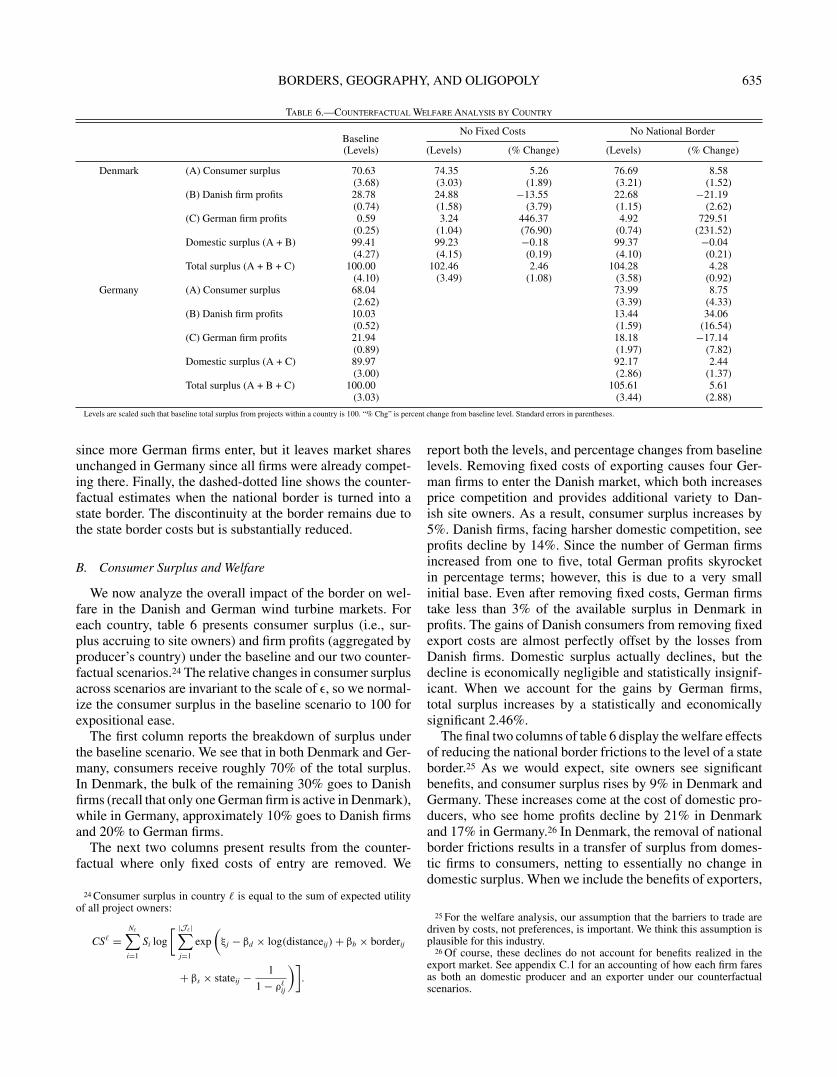
B. Consumer Surplus and Welfare

We now analyze the overall impact of the border on wel-fare in the Danish and German wind turbine markets. Foreach country, table 6 presents consumer surplus (i.e., sur-plus accruing to site owners) and firm profits (aggregated byproducer’s country) under the baseline and our two counter-factual scenarios.24 The relative changes in consumer surplusacross scenarios are invariant to the scale of ε, so we normal-ize the consumer surplus in the baseline scenario to 100 forexpositional ease.

The first column reports the breakdown of surplus underthe baseline scenario. We see that in both Denmark and Ger-many, consumers receive roughly 70% of the total surplus.In Denmark, the bulk of the remaining 30% goes to Danishfirms (recall that only one German firm is active in Denmark),while in Germany, approximately 10% goes to Danish firmsand 20% to German firms.

The next two columns present results from the counter-factual where only fixed costs of entry are removed. We

24 Consumer surplus in country � is equal to the sum of expected utilityof all project owners:

CS� =N�∑i=1

Si log

[ |J� |∑j=1

exp

(ξj − βd × log(distanceij) + βb × borderij

+ βs × stateij − 1

1 − ρ�ij

)].

report both the levels, and percentage changes from baselinelevels. Removing fixed costs of exporting causes four Ger-man firms to enter the Danish market, which both increasesprice competition and provides additional variety to Dan-ish site owners. As a result, consumer surplus increases by5%. Danish firms, facing harsher domestic competition, seeprofits decline by 14%. Since the number of German firmsincreased from one to five, total German profits skyrocketin percentage terms; however, this is due to a very smallinitial base. Even after removing fixed costs, German firmstake less than 3% of the available surplus in Denmark inprofits. The gains of Danish consumers from removing fixedexport costs are almost perfectly offset by the losses fromDanish firms. Domestic surplus actually declines, but thedecline is economically negligible and statistically insignif-icant. When we account for the gains by German firms,total surplus increases by a statistically and economicallysignificant 2.46%.

The final two columns of table 6 display the welfare effectsof reducing the national border frictions to the level of a stateborder.25 As we would expect, site owners see significantbenefits, and consumer surplus rises by 9% in Denmark andGermany. These increases come at the cost of domestic pro-ducers, who see home profits decline by 21% in Denmarkand 17% in Germany.26 In Denmark, the removal of nationalborder frictions results in a transfer of surplus from domes-tic firms to consumers, netting to essentially no change indomestic surplus. When we include the benefits of exporters,

25 For the welfare analysis, our assumption that the barriers to trade aredriven by costs, not preferences, is important. We think this assumption isplausible for this industry.

26 Of course, these declines do not account for benefits realized in theexport market. See appendix C.1 for an accounting of how each firm faresas both an domestic producer and an exporter under our counterfactualscenarios.


however, total surplus increases by 4%. The story in Ger-many is a bit different. Consumer gains outweigh domesticfirm losses in Germany, and domestic surplus increasesby 2%. Essentially, removing border frictions improves theaccess of German site owners to high-productivity Danishfirms and erodes Enercon’s substantial market power in Ger-many. When we include the benefits to Danish exporters,elimination of the border raises surplus in the German marketby a substantial 6%.

We conclude this section with an important disclaimer. Oursecond counterfactual represents a reduction of all nationalborder frictions to the level of only a state border. In real-ity, these frictions are generated by a complex combinationof political, administrative, and cultural differences betweencountries. It is unlikely that any policy initiative would suc-ceed in eliminating these differences completely. Rather, ourfindings illustrate the magnitude of the national border andits effect on firms and consumers in the wind turbine indus-try. Policymakers may view the results as an upper bound onwhat can be accomplished through economic and politicalintegration.

VI. Conclusion

This paper uses spatial microdata to document the impactof fixed and variable border costs while controlling for sev-eral sources of bias that plague analysis of aggregated tradeflows. The model and the detailed geographical informationon manufacturers and projects allow us to better control fordistance costs and differences in competition on either side ofthe border than the existing literature. In addition, the modelenables us to conduct counterfactual analysis on the impactof border frictions on producer and consumer welfare. Wefind that border frictions are substantial; counterfactual anal-ysis indicates that almost 50% of the gap in cross-bordermarket shares can be attributed to national border costs. Ourstudy makes some strides toward identifying the underlyingsources of border frictions. We separately document the roleof a fixed cost to begin exporting and a variable border costfor each exported shipment.

Of course, there is more work to be done. We cannot,for example, separately identify the roles that bureaucratic,linguistic, or cultural differences play in generating borderfrictions. With data from several countries, our model couldeasily be extended to investigate whether cultural or legalsimilarities appear to reduce the costs of crossing nationalboundaries. Moreover, while it is reasonable to attribute bor-der frictions to costs in our setting of a large capital goodtraded in a business-to-business market, in other industries,cross-border differences in preferences—in particular, homebias—may play an important role. This is particularly true inconsumer goods markets.

Finally, the existence of large border frictions within theEuropean wind turbine industry has important policy impli-cations for the EU. Due to growing concerns about climatechange, many governments, including EU members and the

United States, subsidize renewable energy generation. Theefficiency of subsidies in the wind electricity output marketis closely related to the degree of competition in the upstreammarket for wind turbines themselves. If there are substantialfrictions to international trade in turbines, a national sub-sidy to the downstream market may implicitly be a subsidyto domestic turbine manufacturers. This would be againstthe intentions of EU common market policy, which seeks toprevent distortions due to subsidies given by member statesexclusively to domestic firms. In fact, Denmark, which hasone of the most generous wind energy subsidies in Europe,is also home to the most successful European producers ofwind turbines. Our findings of large border frictions in theupstream market imply that harmonizing renewable energytariffs may be necessary to ensure equal treatment of Euro-pean firms in accordance with the principles of the Europeansingle-market project.

REFERENCES

Anderson, J. E., and E. van Wincoop, “Gravity with Gravitas: A Solution tothe Border Puzzle,” American Economic Review 93 (2003), 170–192.

Balistreri, E. J., and R. H. Hillberry, “Structural Estimation and the BorderPuzzle,” Journal of International Economics 72 (2007), 451–463.

Berry, S., “Estimating Discrete-Choice Models of Product Differentiation,”RAND Journal of Economics 25 (1994), 242–262.

Berry, S., J. Levinsohn, and A. Pakes, “Automobile Prices in MarketEquilibrium,” Econometrica 63 (1995), 841–890.

Bresnahan, T. F., and P. Reiss, “Empirical Models of Discrete Games,”Journal of Econometrics 48 (1991), 57–81.

Broda, C., and D. E. Weinstein, “Understanding International Price Differ-ences Using Barcode Data,” NBER working paper 14017 (2008).

Caplin, A., and B. Nalebuff, “Aggregation and Imperfect Competition: Onthe Existence of Equilibrium,” Econometrica 59 (1991), 25–59.

Cosar, A. K., P. L. E. Grieco, and F. Tintelnot, “Bias in Estimating Border-and Distance-Related Trade Costs: Insights from a OligopolyModel,” Economics Letters 126 (2015), 147–149.

Das, S., M. J. Roberts, and J. R. Tybout, “Market Entry Costs, ProducerHeterogeneity and Export Dynamics,” Econometrica 75 (2007),837–873.

Eaton, J., and S. Kortum, “Technology, Geography, and Trade,” Economet-rica 70 (2002), 1741–1779.

Eaton, J., S. Kortum, and F. Kramarz, “An Anatomy of International Trade:Evidence from French Firms,” Econometrica 79 (2011), 1453–1498.

Eizenberg, A., “Upstream Innovation and Product Variety in United StatesHome PC Market,” Review of Economic Studies 81 (2014), 1003–1045.

Engel, C., and J. H. Rogers, “How Wide Is the Border?” American EconomicReview 86 (1996), 1112–1125.

Ericson, R., and A. Pakes, “Markov-Perfect Industry Dynamics: A Frame-work for Empirical Work,” Review of Economic Studies 62 (1995),53–82.

Feenstra, R. C., and J. A. Levinsohn, “Estimating Markups and Mar-ket Conduct with Multidimensional Product Attributes,” Review ofEconomic Studies 62 (1995), 19–52.

Fowlie, M., M. Reguant, and S. P. Ryan, “Market-Based Emissions Reg-ulation and Industry Dynamics,” NBER working paper 18645(2012).

Franken, M., and T. Weber, “Heavy Duty,” New Energy 2008 (2008), 28–37.Goldberg, P. K., and F. Verboven, “The Evolution of Price Dispersion in

the European Car Market,” Review of Economic Studies 68 (2001),811–848.

——— “Market Integration and Convergence to the Law of One Price:Evidence from the European Car Market,” Journal of InternationalEconomics 65 (2005), 49–73.

Gopinath, G., P.-O. Gourinchas, C.-T. Hsieh, and N. Li, “InternationalPrices, Costs and Markup Differences,” American Economic Review101 (2011), 2450–2486.


Gorodnichenko, Y., and L. L. Tesar, “Border Effect or Country Effect?Seattle May Not Be So Far from Vancouver After All,” AmericanEconomic Journal: Macroeconomics 1 (2009), 219–241.

Hillberry, R. H., “Aggregation Bias, Compositional Change, and the BorderEffect,” Canadian Journal of Economics 35 (2002), 517–530.

Hillberry, R., and D. Hummels, “Trade Responses to Geographic Frictions:A Decomposition Using Micro-Data,” European Economic Review52 (2008), 527–550.

Holmes, T. J., “The Diffusion of Wal-Mart and the Economies of Density,”Econometrica 79 (2011), 253–302.

Holmes, T. J., and J. J. Stevens, “Exports, Borders, Distance, and PlantSize,” Journal of International Economics 88 (2012), 91–103.

McCallum, J., “National Borders Matter: Canada-U.S. Regional TradePatterns,” American Economic Review 85 (1995), 615–623.

Melitz, M. J., “The Impact of Trade on Intra-Industry Reallocations andAggregate Industry Productivity,” Econometrica 71 (2003), 1695–1725.

Morales, E., G. Sheu, and A. Zahler, “Gravity and Extended Gravity: UsingMoment Inequalities to Estimate a Model of Export Entry,” HarvardUniversity mimeograph (2014).

Obstfeld, M., and K. Rogoff, “The Six Major Puzzles in InternationalMacroeconomics: Is There a Common Cause?” (pp. 339–412), inBen S. Bernanke and Kenneth Rogoff, eds., NBER MacroeconomicsAnnual 2000, 15 (Cambridge, MA: National Bureau of EconomicResearch, 2001).

Pakes, A., J. Porter, K. Ho, and J. Ishii, “Moment Inequalities and TheirApplication,” Econometrica 83 (2015), 315–334.

Roberts, M. J., and J. R. Tybout, “The Decision to Export in Colombia: AnEmpirical Model of Entry with Sunk Costs,” American EconomicReview 87 (1997), 545–564.

Salvo, A., “Trade Flows in a Spatial Oligopoly: Gravity Fits Well, ButWhat Does It Explain?” Canadian Journal of Economics 43 (2010),63–96.

Sijm, J., “The Performance of Feed-in Tariffs to Promote RenewableElectricity in European Countries,” Energy Resource Center of theNetherlands, ECN-C–02-083 (2002).

Thomadsen, R., “The Effect of Ownership Structure on Prices in Geo-graphically Differentiated Industries,” RAND Journal of Economics36 (2005), 908–929.

BORDERS, GEOGRAPHY, AND OLIGOPOLY:...

Documents

Transcript of BORDERS, GEOGRAPHY, AND OLIGOPOLY:...