Borders, Geography, and Oligopoly:

Evidence from the Wind Turbine Industry∗

A. Kerem CosarChicago Booth

Paul L. E. GriecoPenn State

Felix TintelnotPenn State

February 17, 2012

Abstract

Using a micro-level dataset of wind turbine installations in Denmark and Germany, we estimate astructural oligopoly model with cross-border trade and heterogeneous firms. Our approach separatelyidentifies border-related from distance-related variable costs and bounds the fixed cost of exporting foreach firm. Variable border costs are large: equivalent to roughly 400 kilometers (250 miles) in distancecosts. Fixed costs are also important; removing them would increase German firms market share inDenmark by 10 percentage points. Counterfactual analysis indicates that completely eliminating borderfrictions would increase total welfare in the wind turbine industry by 5 percent in Denmark and 10percent in Germany.

JEL Codes: F14, L11, L20, L60, R12Keywords: border effect, oligopoly, spatial competition, constrained maximum likelihood estimation

∗For their insightful comments, we thank Costas Arkolakis, Lorenzo Caliendo, Allan Collard-Wexler, Steve Davis, JonathanEaton, Charles Engel, Oleg Itskhoki, Kala Krishna, Matthias Lux, Ferdinando Monte, Eduardo Morales, Dennis Novy, RalphOssa, Ayse Pehlivan, Joris Pinkse, Mark Roberts, Andres Rodrıguez-Clare, Alan Spearot, Elie Tamer, Jonathan Vogel, StephenYeaple, Nicholas Ziebarth, and workshop participants at Penn State, Chicago Booth, Boston University, Boston FED, UCLA,U.S. Census Bureau, Ohio State, University of Minnesota, University of Munich, Koc University, EIIT in Purdue University,Midwest Trade Conference, LACEA-TIGN, Conference on Globalization in Denmark, and UECE Lisbon Meetings in GameTheory and Applications. For their valuable discussions with us about the industry, we thank Wolfgang Conrad, RobertJuettner, Alex Kaulen, and Jochen Twele.Correspondence: kerem.cosar@chicagobooth.edu, paul.grieco@psu.edu, fut111@psu.edu.

1

1 Introduction

Since the seminal works of McCallum (1995) and Engel and Rogers (1996), an extensive literature has

documented significant market segmentation across national boundaries. Obstfeld and Rogoff (2001) list

“home bias in trade” as one of the major puzzles in international macroeconomics. Estimated magnitudes

of the border effect are so large that some researchers have suggested they are due to spatial and industry-

level aggregation bias, a failure to account for within-country heterogeneity and geography, and cross-border

differences in market structure.1 To avoid these potentially confounding effects, we use spatial micro-data

from wind turbine installations in Denmark and Germany to estimate a structural model of oligopolistic

competition with border frictions. Our main findings are: (1) border frictions are large within the wind

turbine industry, (2) fixed and variable costs of exporting are both important in explaining overall border

frictions, and (3) these frictions have a substantial impact on welfare.

In contrast to studies that use aggregate trade measures or price indices to estimate a border effect,

this paper focuses on a narrowly defined industry. In addition to being an interesting case for study in its own

right due to the growing importance of wind energy to Europe’s overall energy portfolio, the wind turbine

industry in the European Union (EU) offers an opportunity to examine the effects of national boundaries

on market segmentation. First, we have rich spatial information on the location of manufacturers and

installations. The data are much finer than previously used aggregate state- or province-level data. The

use of disaggregated data allows us to account for actual shipping distances, rather than rely on market-

to-market distances, to estimate border costs. Second, the data contain observations of both domestic and

international trade. We observe active manufacturers on either side of the Danish-German border, some

of whom choose to export and some of whom do not, allowing us to separate fixed and variable border

costs. Third, intra-EU trade is free from formal barriers and subject to wide-ranging efforts to minimize

informal barriers.2 By the Single European Act, national subsidies are directed only toward the generation

of renewable electricity and do not discriminate against other European producers of turbines. The border

costs in this setting are therefore due to factors other than formal barriers to trade.

Despite major formal integration, the data indicate substantial market segmentation between Den-

mark and Germany. Examining the sales of turbines in 1995 and 1996, we find that domestic manufacturers

had a substantially higher market share than did foreign manufacturers. For example, the top five German

manufacturers possessed a market share of 60 percent in Germany and only 2 percent in Denmark. The

1See Hillberry (2002), Hillberry and Hummels (2008), Broda and Weinstein (2008) and Gorodnichenko and Tesar (2009).2All tariffs and quotas between former European Economic Community members were eliminated by 1968. The Single

European Act came into force in 1987 with the objective of abolishing all remaining physical, technical and tax-related barriersto free movement of goods, services, and capital within the EU until 1992. Between 1986 and 1992, the EU adopted 280 piecesof legislation to achieve that goal.

2

market share of Danish producers drops by approximately 30 percent at the border.

What are the sources of cross-national market segmentation? A cursory glance at our data suggests

that national borders affect the decisions of firms to enter the foreign market. To be specific, only one of

the five large German firms exports to Denmark. On the other hand, all five large Danish firms have sales

in Germany, but their market share is substantially lower in the foreign market and drops discontinuously

at the border. The difference in participation patterns across the border can reflect fixed costs faced only by

exporting firms. The change in market share at the border may be generated by differences in competition

(e.g., differences in the set of competitors and their underlying characteristics) or by higher variable costs

for foreign firms.3 To explain differences in market shares along extensive and intensive margins, we propose

a model of cross-border oligopolistic competition that embeds costs for exporting as primitives and controls

for other sources of cross-border differences. This allows us to infer the costs that exporting firms face

and simulate the model by removing these costs to determine their impact on market shares, profits, and

consumer welfare.

In our model, firms are heterogeneous in their production costs, foreign market entry costs, and

distance to project sites. To become active in the foreign country and to be able to export, firms must pay a

fixed border cost specific to them. The model incorporates two types of costs for supplying a project: First,

all firms face a variable cost that increases with the distance between the location where they produce the

turbines—which we take as exogenous—and the location of the project (distance cost). Second, exporters

pay an additional variable border cost for projects in the foreign market. One of our objectives is to gauge

the importance of each type of cost in segmenting the markets.

The model has two stages: In the first stage, turbine producers decide whether or not to export. This

depends on whether their expected profit in the foreign market exceeds their fixed border cost. As a result,

the set of competing firms changes at the border. In the second stage, turbine producers observe the set of

active producers in each market and engage in price competition for each project. A producer’s costs depend

on the location of the project through both distance and the presence of a border between the producer and

the project. For each project, firms choose prices (and hence, markups) on the basis a profit maximization

condition derived from our model. Project managers then face a discrete choice problem, they observe price

bids and pick the producer that maximizes their project’s value. In equilibrium, each firm takes into account

the characteristics of its competitors when choosing its own price. The model thus delivers endogenous

variation in prices, markups, and market shares across points in space. Our data informs us about the

3It may also be that preferences change at the border such that consumers act on a home bias for domestic turbines. Sincein this setting, demand comes from profit maximizing energy producers buying an investment good, we expect that demanddriven home bias are less likely to occur than they would for a consumption good. Within our model, home bias in consumerpreferences cannot be separately identified from border costs.

3

suppliers of all projects. We estimate the model by maximizing the likelihood of correctly predicting these

outcomes.

Our results indicate that there are substantial costs to sell wind turbines across the border between

Denmark and Germany. We find that the variable border costs are roughly equivalent to moving a manufac-

turer 400 kilometers (250 miles) further away from a project site. Given that the largest possible distance

from the northern tip of Denmark to the southern border of Germany is roughly 1,400 kilometers (870 miles),

this is a significant cost for foreign firms. Removing fixed costs of foreign entry, such that all firms compete

on both sides of the border, raises the market share of German firms in Denmark from 2 to 12 percent; also

eliminating variable border costs raises that market share from 12 percent to 22 percent. Counterfactual

analysis provides further insights into the welfare effects of borders. A hypothetical elimination of all border

frictions raises consumer surplus by 10.4 and 15.3 percent in Denmark and Germany, respectively. Removing

border frictions increases profits of foreign firms while reducing those of domestic firms. The net effect is

small in Denmark (producer surplus declines by less than 1 percent) and large in Germany (producer sur-

plus declines by over 6 percent). Overall, consumer gains outweigh producer losses in both countries. Total

surplus increases by 5 percent in Denmark and 10 percent in Germany.

This paper adds to the literature on border effect by estimating border costs within a structural

oligopoly model that controls for internal geography and firm heterogeneity. McCallum (1995) and Anderson

and van Wincoop (2003) use data on interstate, interprovincial, and international trade between Canada

and the United States to document a disproportionately high level of intranational trade between Canadian

provinces and U.S. states after controlling for income levels of regions and the distances between them.

Engel and Rogers (1996) find a high level of market segmentation between Canada and the United States

using price data on consumer goods. Gopinath, Gourinchas, Hsieh, and Li (2011) use data on retail prices

to document large retail price gaps at the border using a regression discontinuity approach. Goldberg and

Verboven (2001, 2005) find considerable price dispersion in the European car market and some evidence that

the markets are becoming more integrated over time.

Rather than examining trade flows or price variation between markets, our dependent variable is

whether a particular firm is contracted to construct a wind turbine at a particular point in space.4 By doing

this, we addresses several critiques raised by the literature. Hillberry (2002) and Hillberry and Hummels

(2008) show that sectoral and geographical aggregation lead to upward bias in the estimation of the border

effect in studies that use trade flows. In a similar fashion, Broda and Weinstein (2008) find that aggregation

of individual goods’ prices amplifies measured impact of borders on price.

4The first strand of papers described above use data on xij =∑N

n=1 qnijp

nij , trade volume between two regions i and j in N

traded goods. The second strand uses information about pnij for a set of tradable goods. This paper uses observation on qnij fora particular tradable good.

4

Holmes and Stevens (2010) emphasize the importance of controlling for internal distances. Our data

enables us to calculate the distances between projects and all potential suppliers. That, in turn, enables

us to separate the impact of distance from the impact of the border. Because manufacturers’ identities are

observed in the data, we are able to control for firm-level heterogeneity.

Our structural model of oligopolistic competition controls for differences in market structure and

competitor costs across space. This approach addresses the concern of Gorodnichenko and Tesar (2009) that

model-free, reduced-form estimates fail to identify the border effect. To highlight the importance of using

disaggregated data and a structural model, Section 6 presents an experiment based on our estimated model

in which we regress price differentials on distances and a border dummy to calculate the implied width of

the border. Consistent with the hypothesis of Gorodnichenko and Tesar (2009), this width is substantially

larger than what our structural model implies.

In summary, our focus on a narrowly defined industry has three major advantages: First, the use of

precise data on locations in a structural model allows for a clean identification of costs related to distance

and border. Second, the model controls for endogenous variation in markups across markets within and

across countries based on changes in the competitive structure across space. By doing that, the model also

provides a framework that can be used to estimate oligopolistic industry models using spatial firm-level data

on purchases. Third, by distinguishing between fixed and variable border costs, we gain a deeper insight,

than we do from studies that use aggregate data, into the sources of border frictions in business-to-business

capital-goods industries, which constitute an important fraction of world trade.

In the following section, we discuss our data and provide background information for the Danish-

German wind turbine industry. We also present some preliminary analysis that is indicative of a border

effect. Section 3 introduces our model of the industry. We show how to estimate the model using maximum

likelihood with equilibrium constraints and present the results in Section 4. In Section 5, we perform

a counterfactual analysis of market shares and welfare by re-solving the model without fixed and variable

border costs. Section 6 uses market-to-market price differentials from our model in a reduced-form regression

to relate our approach to studies that estimate border frictions based on the law of one price. We conclude

in Section 7 with a discussion of policy implications.

2 Industry Background and Data

Encouraged by generous subsidies for wind energy, Germany and Denmark have been at the forefront of what

has become a worldwide boom in the construction of wind turbines. Owners of wind farms are paid for the

electricity they produce and provide to the electric grid. In both countries, national governments regulate

5

Figure 1: Transportation of Wind Turbine Blades

Notes: A convoy of wind turbine blades passing through the village of Edenfield, England. Photo Credit: Anderson (2007)

the unit price paid by grid operators to site owners. These “feed-in-tariffs” are substantially higher than the

market rate for other electricity sources. Important for our study is that public financial support for this

industry is not conditional on purchasing turbines from domestic turbine manufacturers, which would be in

violation of European single market policy. So, it is in the best interest of the wind farm owner to purchase

the turbine that maximizes his or her profits independent of the nationality of the manufacturer.

The project owner’s choice of manufacturer is our primary focus. In the period we study, purchasers

of wind turbines were primarily independent producers, most often farmers or other small investors.5 The

turbine manufacturing industry, on the other hand, is dominated by a small number of manufacturing firms

that both manufacture turbines and construct them on the project owner’s land. Manufacturers usually have

a portfolio of turbines available with various generating capacities. Overall, their portfolios are relatively

5Small purchasers were encouraged by the financial incentive scheme that gave larger remuneration to small, independentproducers such as cooperative investment groups, farmers, and private owners. The German Electricity Feed Law of 1991explicitly ruled out price support for installations in which the Federal Republic of Germany, a federal state, a public electricityutility or one of its subsidiaries held shares of more than 25 percent. The Danish support scheme provided an about 30% higherfinancial compensation for independent producers of renewable electricity (Sijm (2002)). A new law passed in Germany in2000 eliminated the restrictions for public electricity companies to benefit from above market price renumeration of renewableenergy.

6

homogeneous in terms of observable characteristics.6 There could be, however, differences in quality and

reliability that we do not directly observe.

The proximity of the production location to the project site is an important driver of cost differences.

Due to the size and weight of turbine components, oversized cargo shipments typically necessitate road

closures along the delivery route (see Figure 1). Transportation costs range between 6 to 20 percent of total

costs (Franken and Weber, 2008). In addition, manufacturers usually include maintenance contracts as part

of the turbine sale, so they must regularly revisit turbine sites after construction.

2.1 Data

We have constructed a unique dataset from several sources which contains information on every wind farm

developed in Denmark and Germany from 1977 to 2005. The data include the location of each project,

the number of turbines, the total megawatt capacity, the date of grid-connection, manufacturer identity,

and other turbine characteristics, such as rotor diameter and tower heights. We match the project data

with the location of each manufacturer’s primary production facility, which enables the calculation of road-

distances from each manufacturer to each project. This provides us with a spatial source of variation in

manufacturer costs which aids in identifying the sources of market segmentation. A key missing variable in

our data set is transaction price, which necessitates the use of our model to derive price predictions from first

order conditions on profit maximization.7 Rather than infer border costs through price differences, we use

differences in the level of trade; the dependent variable for our analysis is the identify of the manufacturer

chosen to supply each project. Appendix A provides a detailed description of the data.

In this paper, we concentrate on the period from 1995 to 1996.8 This has several advantages. First,

the set of firms was stable during this time period. There are several medium-to-large firms competing in

the market. In 1997, a merger and acquisition wave began, which lasted until 2005. The merger wave,

including cross-border mergers, would complicate our analysis of the border effect. Second, site owners in

this period were typically independent producers. This contrasts with later periods when utility companies

became significant purchasers of wind turbines, leading to more concerns about repeated interaction between

purchasers and manufacturers. Third, this period contains several well-established firms and the national

price subsidies for wind electricity generation had been in place for several years. Prior to the mid-1990s,

the market could be considered an “infant industry” with substantial uncertainty about the viability of firms

6Main observable product characteristics are generation capacity, tower height, and rotor diameter. Distribution of turbinesin terms of these variables is very similar in both countries. Further details are displayed in Table 8 in Appendix A.

7As in most business to business industries, transaction level prices are confidential. Some firms do publish list prices, whichwe have collected from industry publications. These prices, however, do not correspond to relevant final transaction prices dueto site-specific delivery and installation costs.

8Appendix A.4 shows that the evidence on market shares and the border effect is stable in subsequent time periods.

7

Table 1: Major Danish and German Manufacturers

% Market share % Market shareManufacturer Nationality in Denmark in Germany

Vestas (DK) 45.45 12.04Micon (DK) 19.19 8.17Bonus (DK) 12.12 5.05Nordtank (DK) 11.45 4.73WindWorld (DK) 4.38 2.73

Total 92.59 32.72

Enercon (DE) 32.58Tacke (DE) 14.95Nordex (DE) 1.68 7.53Suedwind (DE) 2.37Fuhrlaender (DE) 2.15

Total 94.27 92.3

Notes: Market shares in terms of number of projects installed in 1995-1996.Shares are very similar when projects are weighted by megawatt size.

and downstream subsidies. Fourth, the Danish onshore market saturates after the late 1990s, leaving us with

too little variation at that side of the border.9

In focusing on a two-year period, we abstract away from some dynamic considerations. Although

this greatly simplifies the analysis, it comes with some drawbacks. Most important is that we are unable

to distinguish sunk costs from fixed costs of entering the foreign export market (Roberts and Tybout, 1997;

Das, Roberts, and Tybout, 2007). Because of the small number of firms, we would be unable to reliably

estimate sunk costs and fixed costs separately in any case. Instead, we model the decision to enter a foreign

market as a one-shot game. This decision does not affect the consistency of our variable cost estimates,

whereas our counterfactuals removing fixed costs should be interpreted as removing both sunk and fixed

costs. We also abstract away from dynamic effects on production technologies, such as learning-by-doing

(see Benkard, 2004). Learning-by-doing would provide firms with an incentive to lower prices below a static

profit maximizing level to account for the efficiency gains that will be discovered in producing the turbine.10

Learning-by-doing is less of a concern for the mid-1990s than for earlier years. By 1995, the industry has

matured to the extent that it is reasonable to assume that firms were setting prices to maximize expected

profits from the sale.

Table 1 displays the market shares or the largest five Danish and German firms in both countries.

We take these firms to be the set of manufacturers in our study. All other firms had domestic market shares

9Moreover, after the 1990s a substantial fraction of wind turbine installations are offshore, so road-distance to the turbinelocation is less useful as a source of variation in production costs.

10In some cases, this could even lead firms to sell products below cost. See Besanko, Doraszelski, Kryukov, and Satterthwaite(2010) for a fully dynamic computational model of price-setting under learning-by-doing.

8

Project Supplied by a Danish ProducerProject Supplied by a German Producer

Figure 2: Project Locations

BonusVestas

Micon Nordtank

Wind World

Enercon

Nordex

SuedwindTacke

Fuhrlaender

Figure 3: Producer Locations

below 2 percent, no long-term presence in their respective markets, and did not export. In our model, we treat

these small turbine producers as a competitive fringe. The German and Danish wind turbine markets were

relatively independent from the rest of the world. There was only one firm exporting from outside Germany

and Denmark: A Dutch firm, Lagerwey, which sold to 21 projects in Germany (2.26 percent market share)

and had a short presence in the German market. We include Lagerwey as part of the competitive fringe.

2.2 Preliminary Analysis of the Border Effect

Table 1 and Figure 2 clearly suggest some degree of market segmentation between Germany and Denmark.

Four out of five large German firms—including the German market leader, Enercon—do not have any

foreign presence. That all Danish firms enter Germany whereas only one German firm competes in Denmark

is consistent with the existence of large fixed costs for exporting. Because the German market is much larger

than the Danish market (930 projects were installed in Germany in this period, versus 296 in Denmark—see

the map of projects in Figure 2), these fixed costs can be amortized over a larger number of projects in

Germany.

For those firms that do export, the decline in market share by moving from foreign to domestic

markets may have many different causes. First, market structure changes as the set of firms competing in

9

Figure 4: Market Share of Vestas by Proximity to Primary Production Facility

0.2

.4.6

.81

Mar

ket s

hare

0 75 150

225

300

375

450

525

600

675

750

825

Distance to producer in km.(Market share measured by number of projects)

Notes: Proportion of projects won by Vestas projected on a cubic polynomial of distance to Vestas’s production facility.Regression details are in A.4. Dots are aggregated market shares in bins of 75 km width.

Denmark is smaller than that in Germany. Second, due to transportation costs, foreign firms will have higher

costs than domestic ones simply because projects are likely to be nearer to domestic manufacturing plants.

Finally, there may be some variable border costs, which must be paid for each foreign project produced.

We start by exploring the effect of distance as a potential source of market segmentation. The

impact of distance on firm costs is illustrated by Figure 4. This figure documents Vestas’s declining market

share as the distance from its main manufacturing location increases. Whereas Figure 4 suggests that

costs increase with distance from the manufacturing base, it cannot easily be used to estimate distance

costs. The impact of the border—roughly 160 kilometers from Vestas’s manufacturing plant—confounds the

relationship. Moreover, in an oligopolistic industry, Vestas’s share is a function of not only its own costs but

also those of competitor firms. Our model will jointly solve for the probability that each competing firm wins

a project based on the project’s location in relation to all firms. We are thus able to use the rich variation

in projects across space to estimate the impact of distance on firm costs.

We next employ a regression discontinuity design (RDD) to quantify the effect of the border on

large Danish firms’ market share. Given that wind and demand conditions do not change abruptly, the RDD

uncovers the impact of the border. To implement this, we regress a project-level binary variable that takes

the value one if it is supplied by a large Danish firms and zero otherwise, to a cubic polynomial of distance

from the project to the border, a Germany dummy (to capture the border effect), and interaction terms

10

Figure 5: Market Share of Danish Firms by Proximity to the Border

0.2

.4.6

.81

Mar

ket s

hare

−30

0

−22

5

−15

0

−75 75 15

0

225

300

375

450

525

6000

Distance to border in km.(Distance is negative for Denmark, positive for Germany)

Notes: Regression discontinuity fit of projects supplied by five large Danish firms using a cubic polynomial of distance toborder, a Germany dummy and interaction terms. Regression details are in A.4. Dots are aggregated market shares in bins of75 km width.

(see Appendix A.4 for details). Figure 5 plots the fit of this regression. The border dummy is a statistically

significant −0.295, which is reflected in the sharp drop in the market share of the largest five Danish firms

from around 90 to 60 percent at the border.11

These results give us reason to believe that the border matters in the wind turbine industry. Never-

theless, the discontinuity of the border does not separately identify the effect of changes in market structure

between Germany and Denmark from the impact of variable border costs. Because variable border costs are

incurred precisely at the point where market structure changes, we are unable to use the RDD approach to

separate the two effects. This motivates our use of a structural model. In the following section, we propose

and estimate a model to account for the changes market structure at the border by modeling the competition

for projects as a Bertrand-Nash game.

3 Model

We begin by describing the environment. Denmark and Germany are indexed by ` ∈ {D,G}. Each country

has a discrete finite set of large domestic firms denoted by M` and a local fringe. The number of large

domestic firms is equal to the cardinality of this set, |M`|. Large firms are heterogeneous in their location

11These results are robust to considering projects within various bandwidths of the border, as is standard within the RDDframework. For expository purposes, Figure 5 includes projects in the [-300,600] band.

11

and productivity. There is a fixed number of N` projects in each country, and they are characterized by their

location and size (total megawatt generation capacity). We model cross-border competition in two stages:

In the first stage, large firms decide whether or not they will pay a fixed cost to enter the foreign market.

In the second stage, competing firms bid for each project. Project owners independently choose a turbine

supplier among competing firms. We now present the two stages following backward induction, starting with

the bidding game.

3.1 Project Bidding Game

In this stage, active firms offer a separate price to each project manager, and project managers choose the

offer that maximizes their valuation. The set of active firms is taken as given by all players, as it was realized

in the entry stage. For ease of notation, we drop the country index for the moment and describe the project

bidding game in one country. The set of active, large firms denoted by J and the competitive fringe compete

over N projects. J contains all domestic and foreign firms—if there are any—that entered the market in

the first stage, so M⊆ J .

The per-megawatt payoff function of a project owner i for choosing firm j is

Vij = dj − pij + εij .

The return to the project owner depends on the quality of the wind turbine, dj , the per-megawatt price pij

charged by manufacturer j, and an idiosyncratic choice-specific shock εij .12 It is well known that discrete

choice models only identify relative differences in valuations. We thus model a non-strategic fringe as an

outside option. We denote it as firm 0 and normalize the return as

Vi0 = εi0.

We assume εij is distributed i.i.d. across projects and firms according to the Type-I extreme value distribu-

tion.13 The εi vector is private information to owners who collect project-specific price bids from producers.

The assumption that εi is i.i.d and private knowledge abstracts away from the presence of unobservables,

which are known to the firms at the time they choose prices but are unknown to the econometrician.14 After

12We assume away project-level economies of scale by making price bids per-megawatt. Our data does not enable us toidentify project-level economies of scale. We check whether foreign turbine manufacturers tend to specialize on larger projectsabroad. We find that the average project size abroad is very similar to the average project size at home for each exporting firm.

13Project owners do not have any home bias in the sense that εij ’s are drawn from the same distribution for all producers inboth countries.

14For example, if local politics or geography favors one firm over another in a particular region, firms would account for thisin their pricing strategies, but we are unable to account for this since this effect is unobserved to us. In Appendix B, we addressthe robustness of our estimate to local unobservables of this type.

12

receiving all price bids, denoted by the vector pi, owners choose the firm that delivers them the highest

payoff. Using the familiar logit formula, the probability that owner i chooses firm j is given by

Pr[i chooses j] ≡ ρij(pi) =exp(dj − pij)

1 +∑|J |k=1 exp(dk − pik)

for j ∈ J . (1)

The probability of choosing the fringe is

Pr[i chooses the fringe] ≡ ρi0(pi) = 1−|J |∑j=1

ρij(pi).

Now we turn to the problem of the firm. The cost for firm j to supply project i is a function of its

heterogeneous production cost φj , its distance to the project, and whether or not it is a foreign producer:

cij = φj + βd · distanceij + βb · borderij , (2)

where

borderij =

0 if both i and j are located in the same country,

1 otherwise.

In other words, all firms pay the distance related cost (βd ·distanceij), but only foreign firms pay the variable

border cost (βb · borderij). The distance cost captures not only the cost of transportation but also serves

as a proxy for the cost of post-sale services (such as maintenance), installing remote controllers to monitor

wind farm operations, gathering information about sites further away from the manufacturer’s location,

and maintaining relationships with local contractors who construct turbine towers. The border component

captures additional variable costs faced by foreign manufacturers. This may include the cost of dealing with

project approval procedures in the foreign market and coordinating transportation of bulky components with

various national and local agencies.

Firms engage in Bertrand competition by submitting price bids for projects in the markets in which

they are active.15 They observe the identities and all characteristics of their competitors (i.e., their quality

and marginal cost for each project) except the valuation vector εi. The second stage is thus a static game

with imperfect, but symmetric, information. In a pure-strategy Bayesian-Nash equilibrium, each firm chooses

15Industry experts we interviewed indicated that there was an excess supply of production capacity in the market duringthese years. One indication of this is that many firms suffered from low profitability, sparking a merger wave. Therefore, it isnot likely that capacity constraints were binding in this period.

13

its price to maximize expected profits given the prices of other firms:16

E[πij ] = maxpij

ρij(pij ,pi,−j) · (pij − cij) · Si,

which has the first order condition

0 =∂ρij(pij ,pi,−j)

∂pij(pij − cij) + ρij(pij ,pi,−j),

pij = cij −ρij(pij ,pi,−j)

∂ρij(pij ,pi,−j)/∂pij.

Exploiting the properties of the logit form, this expression simplifies to an optimal mark-up pricing condition:

pij = cij +1

1− ρij(pij ,pi,−j). (3)

The mark-up is increasing in the (endogenous) probability of winning the project and is thus a function

of the set of the firms active in the market and their characteristics. Substituting (3) into (1), we get a

fixed-point problem with |J | unknowns and |J | equations for each project i:

ρij =exp

(dj − cij − 1

1−ρij

)1 +

∑|J |k=1 exp

(dk − cik − 1

1−ρik

) for j ∈ J . (4)

Our framework fits into the class of games for which Caplin and Nalebuff (1991) show the existence of

a unique pure-strategy equilibrium. Using the optimal mark-up pricing condition, the expected profits of

manufacturer j for project i can be calculated as,

E[πij ] =ρij

1− ρijSi.

Potential exporters take expected profits into account in their entry decisions. We turn to the entry game

in the next section.

3.2 Entry Game

Before bidding on projects, an entry stage is played in which all large firms simultaneously decide whether or

not to be active in the foreign market by incurring a firm-specific fixed cost fj . This captures expenses that

16We assume that firms are maximizing expected profits on a project-by-project level. These abstracts away from economicsof density in project locations–i.e., the possibility that by having several projects close together they could be produced andmaintained at a lower cost. We are address the robustness of our model to the presence of economies of density in Appendix B.

14

can be amortized across all foreign projects, such as establishing a foreign sales office, gaining regulatory

approvals, or developing the operating software satisfying the requirements set by national grids.

Let Πj(J−j ∪ j) be the expected profit of manufacturer j in the foreign market where J−j is the

set of active bidders other than j. This is simply the sum of the expected profit of bidding for all foreign

projects:

Πj(J−j ∪ j) =

N∑i=1

E[πij(J−j ∪ j)]. (5)

Manufacturer j enters the foreign market if its expected return is higher than its fixed cost:

Πj(J−j ∪ j) ≥ fj . (6)

Note that this entry game may have multiple equilibria. Following the literature initiated by Bresnahan and

Reiss (1991), we assume that the observed decisions of firms are the outcome of a pure-strategy equilibrium;

therefore, if a firm in our data is active in the foreign market, (6) must hold for that firm. On the other

hand, if firm j is not observed in the foreign market, one we can infer the following lower bound on fixed

export cost:

Πj(J−j ∪ j) ≤ fj . (7)

We use these two necessary conditions to construct inequalities that bound fj from above or from

below by using the estimates from the bidding game to impute the expected payoff estimates of every firm

for any set of active participants in the foreign market.17 We now turn to the estimation of the model.

4 Estimation

Estimation proceeds in two steps: In the first step, we estimate the structural parameters of the project-

bidding game. In the second step, we use these estimates to solve for equilibria in the project-bidding game

with counterfactual sets of active firms to construct the fixed costs bounds. Before proceeding with the

estimation, we must define the set of active firms in every country. Under our model, the set of firms that

have positive sales in a country is a consistent estimate of the active set of firms; therefore, we define a firm

as active in the foreign market if it has any positive sales there.18

17Several papers (e.g., Pakes, Porter, Ho, and Ishii, 2006; Ciliberto and Tamer, 2009) proposed using bounds to constructmoment inequalities for use in estimating structural parameters. Holmes (2011) and Morales, Sheu, and Zahler (2011) appliedthis methodology to the context of spatial entry and trade. Because we observe only a single observation of each firm’s entrydecision, a moment inequality approach is not applicable in our setting.

18Note that every active firm has a positive probability of winning every project. As the number of projects goes to infinity,every active firm wins at least one project. We thus consider firms with zero sales in a market as not having entered in the firststage and exclude them from the set of active firms there.

15

We now reintroduce the country index: ρ`ij is firm j’s probability of winning project i in country

`. The number of active firms in market ` is |J`|, and border`ij equals zero if project i and firm j are both

located in country ` and one otherwise. Substituting the cost function (2) into the winning probability (4),

we get

ρ`ij =exp

(dj − φj − βd · distanceij − βb · border`ij − 1

1−ρ`ij

)1 +

∑|J`|k=1 exp

(dk − φk − βd · distanceik − βb · border`ik − 1

1−ρ`ik

) . (8)

From this equation, one can see that firms’ production costs φj and quality level dj are not separately

identified given our data.19 We thus jointly capture these two effects by firm fixed-effects ξj = dj − φj .

We collect the parameters to estimate into the vector θ = (βb, βd, ξ1, . . . , ξ|MD|+|MG|). We estimate

the model via constrained maximum likelihood, where the likelihood of the data is maximized subject to our

equilibrium constraints. The likelihood function of the project data has the following form:

L(ρ) =∏

`∈{D,G}

N∏i=1

|J`|∏j=1

(ρ`ij)y`ij , (9)

where y`ij = 1 if manufacturer j is chosen to supply project i in country ` and 0 otherwise. θ, together with

the vector of expected project win probabilities ρ, solves the following problem:

maxθ, ρ

L(ρ)

subject to: ρ`ij =exp

(ξj − βd · distanceij − βb · border`ij − 1

1−ρ`ij

)1 +

∑|J`|k=1 exp

(ξk − βd · distanceik − βb · border`ik − 1

1−ρ`ik

)

for ` ∈ {D,G}, i ∈ {1, ..., N`}, j ∈ J .

(10)

Our estimation is an implementation of the Mathematical Programming with Equilibrium Con-

straints (MPEC) procedure proposed by Judd and Su (2011). They show that the estimator is equivalent

to a nested fixed-point estimator in which the inner loop solves for the equilibrium of all markets, and the

outer loop searches over parameters to maximize the likelihood. The estimator therefore inherits all the

statistical properties of a fixed-point estimator. It is consistent and asymptotically normal as the number

of projects tends to infinity. For the empirical implementation, we reformulate the system of constraints in

(10) in order to simplify its Jacobian. In our baseline specification, this is a problem with 12,314 variables

(12 structural parameters and 12,302 equilibrium win probabilities for all firms competing for each project)

19The difference between productivity and quality would be identified if we had data on transaction prices. Intuitively, fortwo manufacturers with similar market shares, high prices would be indicative of higher quality products while low prices wouldbe indicative of lower costs.

16

and 12,302 equality constraints. We describe the details of the computational procedure in Appendix C.

As a robustness check on our baseline specification, we also try an alternative cost specification in

which distance related costs are firm-specific:

c`ij = φj + βdj · distanceij + βb · border`ij .

Note that the difference between this and the baseline specification (2) is that distance cost coefficients are

heterogeneous (βdj vs. βd). This cost function is consistent with Holmes and Stevens (2010), who document

that in U.S. data large firms tend to ship further away, even when done domestically.20 If heterogeneous

shipping costs were present in the wind turbine industry, they might bias our baseline estimate of the border

effect upward through a misspecification of distance costs, since smaller firms would not export due to higher

transport costs instead of the border effect. In the following section, we present results for both specifications.

Once we have recovered the structural parameters, we are able to calculate bounds on the fixed

costs of entry for each firm, fj , using the equations (6) and (7). This involves resolving the model with the

appropriate set of firms while holding the structural parameters fixed at their estimated values. To calculate

standard errors for these bounds, we use a parametric bootstrap procedure.21

4.1 Parameter Estimates

Estimation results are presented in Table 2, with our baseline specification reported in the first column. Both

the cost of crossing the border and the cost of distance are economically and statistically significant. Based

on our estimate, the impact on variable costs associated with exporting are equivalent to an additional 432

kilometers of distance between the manufacturing location and the project site (βb/βd = 0.432). The mean

distance from Danish firms to German projects in our data is 623 kilometers; the distance from German

firms to Danish projects is 602 kilometers. As a consequence, border frictions represent roughly 40 percent

of exporters’ total delivery costs.

To get a sense of the importance of distance-related costs on market outcomes, we calculate the

distance elasticity of the equilibrium probability of winning a project for every project-firm combination.22

For exporters, the median distance elasticity ranges from .95 to 1.40. That is, the median effect of a one

20They rationalize this observation in a model where heterogeneous firms invest in their distribution networks. Productivefirms endogenously face a lower “iceberg transportation cost.”

21To be specific, we repeatedly draw θb from the asymptotic distribution of θ and recalculate the bound each time. Underthe assumptions of the model, the distribution of bound statistic generated by this procedure is a consistent estimate of thetrue distribution.

22The distance elasticities we report are a function of the characteristics of all firms at a particular project site in a veryspecific industry. It is difficult to directly compare these distance elasticities with distance elasticities of aggregated tradevolumes frequently reported in the trade literature that rely on national or regional capital distance proxies (e.g., McCallum(1995); Eaton and Kortum (2002); Anderson and van Wincoop (2003))

17

percent increase in the distance from an exporting firm to a project abroad (holding all other firms’ distances

constant) is a decline of .95 to 1.40 percent in the probability of winning the project. For domestic firms,

the median distance elasticities are lower, ranging from .17 to .83. The difference is due to both the smaller

distances firms must typically travel to reach domestic projects and the impact of the border on equilibrium

outcomes. It appears that distance costs have a significant impact on firm costs and market shares for both

foreign and domestic firms.

As discussed above, the firm fixed effects reflect the combination of differences in quality and pro-

ductivity across firms. We find significant differences between them. It is not surprising that the largest

firms, Vestas and Enercon, have the highest fixed effects. Danish firms generally appear to be stronger than

German ones; although there is significant within-country dispersion. The results suggest that controlling

for heterogeneity across firms is important to correctly estimate the border effect and distance costs.

Since our model delivers expected purchase probabilities for each firm at each project site, we can

use the regression discontinuity approach to visualize how well our model fits the observed data. Figure 6

presents this comparison. The horizontal axis is the distance to the Danish-German border, where negative

distance is inside Denmark. The red (solid) is the raw data fit. This is the same curve as that presented

in Figure 5, relating distance-to border and a border dummy to the probability of a danish firm winning

a project. In particular, this regression does not control for project-to-firm distances. The blue (dotted)

curve is fitted using the expected win probabilities calculated from the structural model. These probabilities

depend explicitly on our estimates of both firm heterogeneity and project-to-manufacturer distances but do

not explicitly depend on distance to the border (as this indirectly affects costs for firms in our model). Note

that predicted win probabilities are nonlinear despite the linearity of costs. This is due to the nonlinear

nature of the model as well as the rich spatial variation of mark-ups predicted by the model. The size of the

discontinuity is somewhat larger using the structural model, although the qualitative result that the border

effect is large is apparent using both methods. Overall, the model fits the data well.

To address our concern that differences in distance costs across firms may affect our estimation

of the border effect, we allow for heterogeneity in distance costs in the second column of Table 2. The

border variable cost coefficient is practically unchanged and remains strongly significant, indicating that our

border effect estimate is not driven by distance cost heterogeneity. Turning to the distance costs themselves,

most firms, particularly the larger ones, have distance costs that are close to our homogenous distance

cost estimate. It does not appear that small firms have systematically higher distance costs. The smallest

firm in our data, Suedwind, is estimated to be distance loving; this firm is based in Berlin, but has built

several turbines in the west of Germany.23 While a formal likelihood ratio test rejects the null hypothesis of

23Nordex, who is also located in the east of Germany, also has a negative coefficient, but it is statistically insignificant.

18

Table 2: Maximum Likelihood Estimates

Baseline HeterogeneousDistance Costs

Border Variable Cost, βb 0.869 0.867(0.219) (0.239)

Distance Cost (100km), βd 0.201(0.032)

Bonus (DK) 0.169(0.066)

Nordtank (DK) 0.277(0.073)

Micon (DK) 0.134(0.051)

Vestas (DK) 0.287(0.049)

WindWorld (DK) 0.016(0.068)

Enercon (DE) 0.296(0.063)

Fuhrlaender (DE) 1.794(0.236)

Nordex (DE) -0.071(0.087)

Suedwind (DE) -0.231(0.104)

Tacke (DE) 0.103(0.071)

Firm Fixed Effects, ξj

Bonus (DK) 2.473 2.332(0.223) (0.297)

Nordtank (DK) 2.526 2.811(0.229) (0.326)

Micon (DK) 3.097 2.786(0.221) (0.268)

Vestas (DK) 3.805 4.180(0.215) (0.265)

WindWorld (DK) 1.735 0.818(0.273) (0.418)

Enercon (DE) 3.533 3.859(0.175) (0.270)

Fuhrlaender (DE) 0.330 3.305(0.263) (0.506)

Nordex (DE) 1.782 0.683(0.203) (0.400)

Suedwind (DE) 0.537 -1.188(0.270) (0.510)

Tacke (DE) 2.389 2.104(0.177) (0.263)

Log-Likelihood -2363.00 -2315.82N 1226 1226

Notes: Standard errors in parentheses.

19

Figure 6: Model Fit: Expected Danish Market Share by Distance to the Border

0.2

.4.6

.81

Mar

ket s

hare

−30

0

−22

5

−15

0

−75 75 15

0

225

300

375

450

525

6000

Distance to border in km.

Data Baseline Model

(Distance is negative for Denmark, positive for Germany)

Notes: Data line is the same as in Figure 5. The model line is the regression discontinuity fit of probability of winning eachproject by Danish firms on a cubic polynomial of distance to border, Germany dummy, and interaction terms.

homogeneous distance costs, the estimation results indicate that heterogeneous distance costs are not driving

cross-border differences in this industry. Therefore, we use our baseline specification for the counterfactual

analysis below.

4.2 Fixed Cost Bounds

Not all firms enter the foreign market; rather, firms optimally choose whether or not to export by weighing

their fixed costs of entry against the expected profits from exporting. Hence, firm-level heterogeneity in

profits, fixed costs, or both is necessary to rationalize the fact that different firms make different exporting

decisions. Since our model naturally allows for heterogeneity in firm operating profits, this section considers

whether heterogeneity in firms’ fixed costs of exporting are also needed to rationalize observed entry decisions.

Since we only observe a single export decision for each firm, fixed costs are not point identified.

Nevertheless, the model helps to place a bound on them. Firms optimally make their export decision based

on the level of fixed costs of foreign entry and on the operating profits they expect in the export market as

described in Section 3.2. Based on the parameter estimates in Table 2, we can derive counterfactual estimates

of expected operating profits for any set of active firms in the Danish and German markets. Therefore, we

can construct an upper bound on fixed costs for firms entering the foreign market using (6), and a lower

bound on fixed costs for firms that stay out of the foreign market using (7). While the scale of these bounds

20

Table 3: Export Fixed Cost Bounds (fj)

Lower Upper

Bonus (DK) 47.55(19.52)

Nordtank (DK) 43.29(8.91)

Micon (DK) 80.13(13.62)

Vestas (DK) 164.32(23.60)

WindWorld (DK) 17.35(3.93)

Enercon (DE) 22.32(4.87)

Fuhrlaender (DE) 0.66(0.32)

Nordex (DE) 6.33(1.82)

Suedwind (DE) 1.26(0.45)

Tacke (DE) 7.24(1.71)

Notes: Scale is normalized by the variance of ε. Stan-dard errors in parentheses.

is normalized by the extreme-value error term, comparing them across firms gives us some idea of the degree

of heterogeneity in fixed costs.

Table 3 presents the estimates of fixed cost bounds for each firm. The intersection of the bounds

across all firms is empty. For example, there is no single level of fixed costs that would simultaneously justify

WindWorld entering Germany and Enercon not entering Denmark; hence, some heterogeneity in fixed costs

is necessary to explain firm entry decisions.

One possibility is that fixed cost for entering Germany differ from those for entering Denmark. Since

all Danish firms enter the Danish market, any fixed cost below 17.35 (the expected profits of WindWorld for

entering Germany) would rationalize the observed entry pattern. In Germany however, the lower and upper

bound of Enercon and Nordex have no intersection. Some background information about Nordex supports

the implication of the model that Nordex may be subject to much lower costs than Enercon to enter into

the Danish market. Nordex was launched as a Danish company in 1985 but shifted its center of business

and production activity to Germany in the early 1990s. As a consequence, Nordex could keep a foothold in

the Danish market at a lower cost than could the other German firms, which would need to form contacts

21

with Danish customers from scratch.24

Of course, the Nordex anecdote also highlights some important caveats with regard to our bounds.

By assuming a one-shot entry game, we are abstracting away from entry dynamics. If exporting is less costly

to continue than to initiate, then the bounds we calculate—which consider only profits from operating in

1995 and 1996—will be biased downward. Data limitations, particularly the small number of firms, prevent

us from extending the model to account for dynamic exporting decisions along the lines of Das, Roberts, and

Tybout (2007). Nevertheless, our results illustrate the degree of heterogeneity in fixed costs that is necessary

to explain entry patterns.25

5 Border Frictions, Market Segmentation, and Welfare

We now use the model to study the impact of border frictions on national market shares, firm profits, and

consumer welfare. We perform a two-step counterfactual analysis. In the first step, we eliminate fixed costs

of exporting, which results in all firms entering the foreign market. We then re-solve the model for this new

set of active firms, keeping in place variable costs incurred at the border.26 This counterfactual allows us to

examine the importance of the change in the competitive environment at the border. In the second step, we

additionally remove the variable cost of the border by setting βb equal to zero. This eliminates all border

frictions such that the only sources of differing market shares across national boundaries are plant-to-project

distances and firm heterogeneity.27 While the results of this experiment constitute an estimate of what can

be achieved if border frictions could be entirely eliminated, it is important to keep in mind that natural

barriers, such as different languages, will be difficult to eliminate in practice.

5.1 Market Shares and Segmentation

We begin our analysis by considering how national market shares in each country react to the elimination

of border frictions. Furthermore, because market shares are directly observed in the data, the baseline

model’s market share estimates can also be used to assess the fit of our model to national level aggregates.

24Because of Nordex’s connection to Denmark, we perform a robustness check on our variable border cost estimate by re-estimating the model allowing Nordex to sell in Denmark without having to pay the border variable cost. The border costestimate increases in this specification, but the difference is not statistically significant. Since Nordex is the only exportingGerman firm, this robustness check also serves as a check on our specification of symmetric border costs. See Balistreri andHillberry (2007) for a discussion of asymmetric border frictions.

25It is important to note that the variable cost estimates presented in Table 2, as well as the counterfactual results below, arerobust to dynamic entry as long as firm pricing decisions have no impact on future entry decisions. This assumption is quitecommon in the literature on structural oligopoly models, e.g., Ericson and Pakes (1995).

26We implicitly assume that the change in market structure does not induce domestic firms to exit the industry, or new firmsto be created.

27We eliminate first fixed border costs and then variable costs because changes in variable border costs when fixed costs arestill positive could induce changes in the set of firms that enter foreign markets. Because they are not point identified, we areunable to estimate fixed border costs. Even with reliable estimates, the entry stage with positive fixed costs is likely to resultin multiple equilibria.

22

Table 4: Counterfactual Market Shares of Large Firms (%)

Data Baseline No Fixed No BorderEstimates Costs

DenmarkDanish Firms 92.57 92.65 83.95 74.26

(1.52) (2.26) (3.64)

German Firms 1.69 2.18 11.56 21.94(0.60) (2.05) (3.88)

GermanyDanish Firms 32.37 32.42 32.42 49.32

(5.42) (5.42) (7.55)

German Firms 59.57 59.24 59.24 44.90(3.93) (3.93) (5.80)

Notes: Market share measured in projects won. Standard errors in parentheses.

Table 4 presents the market share of the major firms of Denmark and Germany in each country, with the

fringe taking the remainder of the market. Comparing the first two columns, the baseline predictions of the

model closely correspond to the observed market shares. All of the market shares are within the 95 percent

confidence interval of the baseline predictions, which suggests that the model is a good fit.

In the third column, we re-solve the model by eliminating fixed costs of exporting and keeping the

variable border cost in place. In response, the four German firms that previously competed only domestically

start exporting to Denmark. As a result, the market share of German firms in Denmark rises more than 10

percentage points.28 Danish firms, however, still maintain a substantial market share advantage in their home

market. Since all five large Danish firms already compete in Germany, there is no change in market shares

on the German side of the border when fixed costs of exporting are removed.29 The difference in response

to the elimination of fixed costs between the Danish and German markets is obvious, but instructive. The

reduction or elimination of border frictions can have very different effects based on market characteristics. In

our case, because there are more projects in Germany than in Denmark, the return to entry is much larger

in Germany. This may be one reason why we see more Danish firms entering Germany than vice versa.30

As a result, reducing fixed costs of exporting to Germany has no effect on market outcomes, whereas the

impact of eliminating fixed cost of exporting to Denmark is substantial.

The fourth and final column of Table 4 displays the model prediction of national market shares if

the border were entirely eliminated. In addition to setting fj equal for all firms, we also eliminate variable

28For space and clarity, we do not report standard errors of changes in market shares in Table 4. All of the (non-zero) changesin market shares across counterfactuals are statistically significant.

29Because of this duplication, we simply omit the column which removes fixed cost of entry in Germany in the tables below.30This argument assumes fixed costs of exporting are of the same order of magnitude for both countries, which appears to

be the case.

23

border costs by setting βb equal to zero.31 This results in a large increase in imports on both sides of the

border. The domestic market share of Danish firms falls from 92.6 percent to 74.3 percent. The domestic

market share of large Danish firms remains high due to firm heterogeneity and the fact that they are closer

to Danish projects. In Germany, a slight majority of projects imports Danish turbines once the border

is eliminated, which reflects the strength of Danish firms (especially Vestas) in the wind turbine industry.

On both sides of the border, we see an approximate 20 percent increase in import share when the national

boundary is eliminated.

Overall, our results indicate that border frictions generate significant market segmentation between

Denmark and Germany. As a back of the envelope illustration, consider the difference between the market

share of Danish firms in the two markets. The gap in the data and baseline model is roughly 60 percentage

points. Not all of this gap can be attributed to border frictions since differences in transportation costs

due to geography are also responsible for part of the gap. However, when we remove border frictions, our

counterfactual analysis indicates that the gap shrinks to 25 percentage points. More than half of the market

share gap is thus attributable to border frictions. When considering the sources of border frictions, we find

that removing fixed costs of exporting alone accounts for one-third of the market share gap that is attributed

to border frictions, while the remaining two-thirds are realized by removing both fixed and variable border

frictions. Since fixed and variable costs interact, the overall impact of border frictions cannot be formally

decomposed into fixed and variable cost components. We take these results as evidence that both fixed and

variable border frictions are substantial sources of market segmentation.

In addition to national market share averages, our model allows us to examine predicted market

shares at a particular point in space. Using the RDD approach describe above, Figure 7 visualizes the impact

of the counterfactual experiments. The blue (dashed) line represents expected market shares baseline model,

and is identical to that presented in Figure 6. The red (dotted) line displays counterfactual expected market

shares when fixed border costs are removed. This reduces domestic market share of Danish firms since

more German firms enter, but leaves market shares unchanged in Germany since all firms were already

competing there. Finally, the green (dashed-dotted) line shows the counterfactual estimates when all border

costs are eliminated. The discontinuity at the border is entirely eliminated, and only the impact of firm-to-

manufacturer distances cause differences in market share on either side of the border.32

31Because adjustments to variable costs may result in a change in firms optimal entry decisions, we are unable to perform acounterfactual eliminating variable border costs alone.

32The kink at the boundary is an artifact of interaction terms in the RDD which implies that we estimate either side ofthe border as a separate cubic polynomial in distance to the border. The bottom line is that there is no discontinuity at theboundary when all border effects are removed.

24

Figure 7: Counterfactuals: Expected Danish Market Share by Distance to the Border

0.2

.4.6

.81

Mar

ket s

hare

−30

0

−22

5

−15

0

−75 75 15

0

225

300

375

450

525

6000

Distance to border in km.

Baseline Model No fixed costs No border

(Distance is negative for Denmark, positive for Germany)

Notes: Regression discontinuity fit of projects won by Danish firms on a cubic polynomial of distance to border, Germanydummy, and interaction terms.

5.2 Firm Profits

We now turn to an analysis of winners and losers from border frictions, starting with individual firms. Table

5 presents the level of operating profits predicted by our model under the baseline and two counterfactual

scenarios.33 While the scale of these profit figures is arbitrary, they allow for comparison both across firms and

across scenarios. The table separates profits accrued in Germany and Denmark for each firm. For example,

in the baseline scenario, we see that Bonus made 47.06 in profits in Denmark, and 47.55 in Germany. If the

border were removed entirely, Bonus’s profits in Denmark would fall to 34.83, while their profits in Germany

would rise to 75.46. On overall, Bonus would see its total profits increase as a result of the elimination of

border frictions, as gains in Germany would more than offset loses from increased competition in Denmark.

From Melitz (2003), we would predict that small firms tend to loose from trade liberalization while

large firms tend to gain. It is true that when fixed costs are eliminated, the large German firms—Enercon

and Tacke—take the lion’s share of the gains. However, we find that all German firms—even the largest firm,

Enercon—would loose from the entire elimination of the Danish-German border. Underlying this result is the

significant size asymmetry between Germany and Denmark. The losses German firms face due to increased

competition in the larger German market overwhelm all gains they receive from frictionless access to the

Danish market. Our model estimates Danish firms to be highly productive, so eliminating the border is

33Operating profits are calculated according to (5) and do not include fixed costs.

25

Table 5: Baseline and Counterfactual Profit Estimates

Denmark Germany

Baseline No Fixed No Border Estimates No BorderCosts

Bonus (DK) 47.06 41.02 34.83 47.55 75.46(13.00) (11.98) (10.71) (19.52) (28.88)

Nordtank (DK) 44.70 38.98 33.11 43.29 68.72(4.97) (4.50) (4.19) (8.91) (13.73)

Micon (DK) 82.76 72.63 62.07 80.13 126.74(7.36) (6.80) (6.75) (13.62) (21.14)

Vestas (DK) 156.96 139.46 120.69 164.32 256.08(14.60) (12.46) (11.83) (23.60) (37.23)

WindWorld (DK) 20.73 18.13 15.44 17.35 27.59(3.19) (2.76) (2.49) (3.93) (6.32)

Enercon (DE) 21.46 42.56 428.91 305.06(4.54) (9.37) (48.68) (53.60)

Fuhrlaender (DE) 0.57 1.14 17.31 11.98(0.26) (0.56) (4.20) (3.28)

Nordex (DE) 6.33 5.43 10.79 75.69 51.24(1.82) (1.48) (2.45) (15.15) (13.20)

Suedwind (DE) 1.09 2.16 21.74 14.85(0.37) (0.78) (5.23) (3.90)

Tacke (DE) 6.47 12.93 151.86 104.83(1.42) (3.19) (16.60) (17.33)

Notes: Scale is normalized by variance of ε. Standard errors in parentheses.

quite costly to German incumbents. In addition, variable border frictions are estimated to be so high that

even a small Danish exporter like WindWorld becomes much more competitive in Germany when they are

removed. Despite being a relatively small player, WindWorld gains from the elimination of border frictions

since increased profits in the larger Germany market outweigh its losses at home. However, WindWorld’s

gains are insignificant when compared to the gains of the large Danish firms, such as Vestas. Overall, we

find that because a German firm’s domestic market is considerably larger than its export market, border

frictions protect the profit of German firms over those of Danish firms.

5.3 Consumer Surplus and Welfare

Finally, we analyze the overall impact of the border on welfare in the Danish and German wind turbine

markets. For each country, Table 6 presents consumer surplus (i.e., surplus accruing to site owners) and firm

profits (aggregated by country) under the baseline and our two counterfactual scenarios. For comparison

purposes, we normalize welfare such that baseline total surplus for each country is equal to 100.34 We define

34Because of its larger size, the total surplus in Germany is much larger than in Denmark, cross country comparisons of totalsurplus are available by request.

26

Table 6: Counterfactual Welfare Analysis by Country

Baseline No Fixed Costs No Border(Levels) (Levels) (% Chg) (Levels) (% Chg)

Denmark

(A) Consumer Surplus 70.15 73.46 4.72 77.42 10.36(4.94) (4.97) (1.03) (5.38) (2.19)

(B) Danish Firm Profits 29.33 25.83 -11.92 22.16 -24.44(0.54) (0.74) (2.26) (1.26) (4.47)

(C) German Firm Profits 0.53 2.91 452.99 5.79 999.18(0.15) (0.55) (122.97) (1.13) (297.29)

Domestic Surplus (A+B) 99.47 99.29 -0.18 99.58 0.10(5.17) (5.11) (0.07) (5.09) (0.25)

Total Surplus (A+B+C) 100.00 102.21 2.21 105.37 5.37(5.09) (5.07) (0.51) (5.39) (1.28)

Germany

(A) Consumer Surplus 68.99 79.57 15.34(6.42) (8.30) (1.90)

(B) Danish Firm Profits 10.43 16.41 57.27(1.59) (2.41) (4.96)

(C) German Firm Profits 20.58 14.44 -29.84(1.86) (2.31) (5.62)

Domestic Surplus (A+C) 89.57 94.01 4.96(5.78) (6.68) (1.39)

Total Surplus (A+B+C) 100.00 110.42 10.42(6.72) (8.59) (1.77)

Notes: Levels are scaled such that baseline total surplus from projects within a country is 100. “% Chg” ispercent change from baseline level. Standard errors in parentheses.

domestic surplus as the total surplus in the country that accrues to consumers and domestic firms.

The first column reports the breakdown of surplus under the baseline scenario, we see that in both

Denmark and Germany, consumers receive roughly 70 percent of the total surplus. In Denmark, the bulk

of the remaining 30 percent goes to Danish firms (recall that only one German firm is active in Denmark),

while in Germany, approximately 10 percent goes to Danish firms and 20 percent to German firms.

The next two columns present results from the counterfactual where only fixed costs of entry are

removed. As discussed above, this counterfactual only affects the Danish market outcomes, since all Danish

firms already sell in Germany in the baseline scenario. We report both surplus levels, and the percentage

change from the baseline level. Note that, because of the correlation in the level estimates due to the

uncertainty in firm fixed effects, the percent change estimates are much more precise than a naıve comparison

of the level estimates would suggest. Removing fixed costs of exporting causes four German firms to enter

the Danish market, which both increases price competition and provides additional variety to Danish site

owners. As a result, consumer surplus increases by 4.72 percent. Danish firms, facing harsher domestic

competition, see profits decline by 11.92 percent. Since the number of German firms increased from one

to five, total German profits skyrocket in percentage terms, however this is due to a very small initial

27

base. Even after removing fixed costs, German firms take less than three percent of the available surplus in

Denmark in profits. The gains of Danish consumers from removing fixed export costs are almost perfectly

offset by the loses from Danish firms. Domestic surplus actually declines by a statistically significant but

economically negligible amount. When we account for the gains by German firms, total surplus increases by

the statistically and economically significant 2.21 percent.

The final two columns of Table 6 display the welfare effects of removing border frictions entirely. As

we would expect, site owners see significant benefits, and consumer surplus rises by 10.36 percent in Denmark

and 15.34 percent in Germany. The increase in Denmark is more than twice as high as the increase realized

from only removing fixed border costs. These increases come at the cost of domestic producers, who see

home profits decline by 24.44 percent in Denmark and 29.84 percent in Germany.35 In Denmark, the removal

of border frictions results in a transfer of surplus from domestic firms to consumers, netting to essentially

no change in domestic surplus. When we include the benefits of exporters, however, total surplus increases

by 5.37 percent. The story in Germany is a bit different. Consumer gains outweigh domestic firm losses in

Germany and domestic surplus increases by 4.96 percent. Essentially, removing border frictions improves

German site owners access to high-productivity Danish firms and erodes Enercon’s substantial market power

in Germany. When we include the benefits to Danish exporters, elimination of the border raises surplus in

the German market by a substantial 10.42 percent.

We conclude this section by repeating an important disclaimer. Our counterfactuals represent com-

plete elimination of the border effect. In reality, the border effect is generated by a complex combination of

political, administrative, and cultural differences between countries. Therefore, it is unlikely that any policy

initiative would succeed in completely eliminating the border. Rather, our findings illustrate the magnitude

of the border and its effect on firms and consumers in the wind turbine industry. Policy makers may view

the results as an upper bound on what can be accomplished through political integration.

6 Reduced-Form Estimation of the Structural Border

Several studies have used a no-arbitrage condition to motivate estimates of border frictions. In contrast, we

have explicitly modeled border costs within an oligopolistic framework, without appealing to the law of one

price directly. In order to highlight how these approaches may differ, this section uses our model-generated

prices in a reduced-form regression that relates price differentials across space to distance and the border.

Our goal is to compare the implied width of the border from this exercise with the structural estimate on

35Of course, these declines do not account for benefits realized in the export market. See Table 5 for an accounting of howeach firm fairs as both an domestic producer and an exporter under our counterfactual scenarios.

28

variable border costs from Section 4.1 and identify the sources of discrepancies between the two.36

The regression is in the spirit of Engel and Rogers (1996) and the ensuing literature that estimate

the border effect using within- and cross-country prices. In this line of inquiry, the border effect is the

additional price dispersion brought about by the national boundaries. The researcher starts with a panel

data pjkt of prices for identical, tradable goods indexed by j measured in locations indexed by k. In order

to test deviations from the relative version of the law of one price, she collapses the time series variation to

cross-sectional variation in the volatility of prices across goods and locations. To be specific, let σjk` represent

the standard deviation of period-to-period changes in the relative price over time of good j in locations k

and `.

σjk` = std

{pjktpj`t−pjkt−1

pj`t−1

}Tt=1

A low σjk` means that shocks to the price of good j in one location are quickly transmitted to the other.

Thus, the higher the volatility, the weaker is the law-of-one price between cities k and `. A typical regression

a la Engel and Rogers (1996) is as follows:

σjk` = δjd · ln distancek` + δjb · borderk` + δjk + δj` + εjk`,

where distancek` is the distance between locations k and `, and borderk` = 1 if k and ` are in the different

countries. Location fixed effects are included to control for city-specific differences that impact price volatility,

such as different seasonal patterns or data collection techniques. The border effect for good j is then

interpreted in terms of the distance equivalent of the border dummy coefficient:

Border Effectj = exp(δjb/δjd).

Rather than consider volatility, our framework allows us to estimate the border effect from the

absolute version of the law of one price using price differentials directly.37 In our thought experiment, we

treat the border width of 432 kilometers estimated in Section 4.1 as its “true” value. An econometrician trying

to recover it from a statistical model observes prices pjk for the same turbine j in different locations k, the

distances between locations (distancek`) but not the distances between locations and producers (distancekj).

This is a good description of the information set used by researchers who estimate reduced-form regressions

36We compare this estimate to the variable border cost because the fixed border cost is sunk when firms set prices.37Engel and Rogers (1996) do not test the absolute law of one price directly because of two reasons. First, measured prices

are typically indices rather than actual prices. Second, price differentials can arise due to differences in local market conditionsand input costs that are not traded.

29

Table 7: Border Effect Estimates from Reduced-Form Estimation

δb/δd

Firm in km

Bonus 741.98Nordtank 857.95Micon 781.16Vestas 516.61WindWorld 1092.08Nordex 3472.55

depicted above. We follow their practice and estimate a similar OLS regression, adapted to our framework:

|pjk − pj` | = δjd · distancek` + δjb · borderk` + δjk + δj` + εjk`. (11)

Our data allows us to calculate distances between each project pair (k, `). Again, the border dummy

equals one if two projects are in different countries. Price pjk is the endogenous equilibrium price bid of firm

j for project k given in (3) in Section 3.1. We report the implied border effect from this regression in Table

7. Evidently, this exercise overestimates the border effect in our model for all producers.38 For Danish firms,

estimates vary between 1.2 to 2.5 times the “true” value of 432 kilometers. The bias is much higher for the

German firm, Nordex.

To gain intuition on the sources of this overestimation, contrast (11) with the price difference implied

by our structural model using our estimates (βd, βb, ρkj) in expressions (2) and (3):

|pjk − pj` | =

∣∣∣βd(distancekj − distance`j)

+ βb(borderkj − border`j

)+( 1

1− ρkj− 1

1− ρ`j

)∣∣∣ (12)

The three terms in this equation reflect the sources of producer-level spatial price differentials in our model:

differences in project-to-producer distances are captured by the first term, differences in border frictions for

each project are captured by the second term, and differences in project-specific mark-ups due to variation

in competitive structure across space are captured by the last term. Note that the firm competitiveness

parameter has canceled out through taking differences.

When we compare this data generating process with equation (11), it is apparent that the linear

reduced-form regression is misspecified. In the structural equation (12), price differentials are generated by

38The overestimation is robust to whether or not we include location fixed effects, which are included in the reported results.In the underlying regressions, distance and border coefficients are statistically significant at .01 level for all producers. Thedetailed regression results are available from authors upon request.

30

the absolute value of several differences in project-to-producer distances, destination countries, and mark-ups,

whereas (11) is a linear function of related, but different, parameters. While trying to emulate this model-

based expression, equation (11) suffers from two additional problems: First, using project-to-project distances

(distancek`) instead of the differences in project-to-producer distances differences (distancekj − distance`j)

leads to (non-classical) measurement error. The triangle inequality implies that the actual difference of

the project-to-producer distances is less than the project-to-project distances. This would tend to bias the

estimate of δd towards zero relative to the distance parameter βd in (12).39 Second, (11) suffers from omitted

variable bias due to the mark-up differentials being left out. Note that the vector of location fixed effects

included in the regression cannot properly characterize the the mark-up differences between project-pairs,

since those dummies would capture information about levels instead of differences. Since markup differences

are likely to be correlated with the border dummy, this would tend to bias δb upwards due to an endogeneity

problem. The combined result is the border effect estimates δb/δd in Table 7 are higher than their structural

analogue, βb/βd.

While our thought experiment focuses on price deviations directly rather than price volatility, it is

easy to see that the linear specification error, measurement error and omitted variable bias would arise when

volatility measures are the dependent variable. The findings of this section resonate with Gorodnichenko

and Tesar (2009) who argue that model-free border-effect regressions fail to identify border frictions when

there is within-country price dispersion due to spatial variation in competition and transportation costs.

Moreover, we show the importance of using disaggregated data—in our case the knowledge of manufacturing

locations—to properly control for variation in distance costs and markups. These issues apply to a large

range of industries in which specific producers operate in only a few locations and the set of active firms is

different on either side of the border.

7 Conclusion

This paper uses transaction-level data for a specific industry to document the impact of fixed and variable

border costs while controlling for several sources of bias that plague analysis of aggregated trade flows.

The model and the detailed geographical information on manufacturers and projects allow us to better

control for distance costs and spatial differences in competition on either side of the border than the existing

literature. The model combines conventional tools from the literature into a novel approach to analyze

39The triangle inequality discrepancy explains why the measured effect is so much higher for Nordex in Table 7. Danish firmsare all located at the north end of the set of projects. Hence, project-to-project distance is a better proxy for the distancedifferential, since the majority of projects are south of their manufacturing facility. Nordex, however, is more centrally located.As a result, two separate projects in Denmark and Germany that are equidistant to Nordex, and thus have a low firm-to-projectdistance differential will have a high project-to-project distance. Nordex’s distinctively higher border effect estimate is thus inpart due to a poorer distance proxy for many project pairs.

31

spatial oligopolistic competition in a multi-country setting.

The large differences in national market shares in the wind turbine industry between Denmark and

Germany arise not only through costs associated with distance, but also through barriers to foreign market

entry and higher variable costs associated with crossing the border. These border costs are substantial;

more than 50 percent of gap in cross-border market shares can be attributed to them. Our results also

indicate that the welfare gains from a hypothetical removal of all border frictions between Germany and

Denmark—including barriers that are difficult to remove, such as language—are substantial. We cannot,

however, separately identify the roles that bureaucratic, language, or cultural differences play in generating

border frictions.

Nonetheless, the existence of large border frictions within the European wind turbine industry has

important policy implications for the EU. Due to growing concerns about climate change, many governments,

including EU members and the United States, subsidize renewable energy generation. The efficiency of

subsidies in the wind electricity output market is closely related to the degree of competition in the upstream

market for wind turbines themselves. If there are substantial frictions to international trade in turbines, a

national subsidy to the downstream market may implicitly be a subsidy to domestic turbine manufacturers.

This is against the intensions of EU common market policy, which seeks to prevent distortions due to subsidies

given by member states exclusively to domestic firms. In fact, Denmark, which has one of the most generous

wind energy subsidies in Europe, is also home to the most successful European producers of wind turbines.

Given our findings of large border frictions in the upstream market, EU members may wish to harmonize

renewable energy tariffs to ensure equal treatment of European firms in accordance with the principles of

the European single market project.

32

References

Anderson, J. E., and E. van Wincoop (2003): “Gravity with Gravitas: A Solution to the Border Puzzle,”The American Economic Review, 93(1), pp. 170–192.

Anderson, P. (2007): “Scout Moor Wind Farm Under Construction,” http://www.geograph.org.uk/

gallery/scout_moor_wind_farm_under_construction_6568.

Balistreri, E. J., and R. H. Hillberry (2007): “Structural estimation and the border puzzle,” Journalof International Economics, 72(2), 451–463.

Benkard, C. L. (2004): “A Dynamic Analysis of the Market for Wide-Bodied Commericial Aircraft,”Review of Economic Studies, 71, 581–611.

Besanko, D., U. Doraszelski, Y. Kryukov, and M. Satterthwaite (2010): “Learning-by-Doing,Organizational Forgetting, and Industry Dynamics,” Econometrica, 78(2), 453–508.

Bresnahan, T. F., and P. Reiss (1991): “Empirical Models of Discrete Games,” Journal of Econometrics,48(1), 57–81.

Broda, C., and D. E. Weinstein (2008): “Understanding International Price Differences Using BarcodeData,” NBER Working Papers 14017, National Bureau of Economic Research, Inc.

Caplin, A., and B. Nalebuff (1991): “Aggregation and Imperfect Competition: On the Existence ofEquilibrium,” Econometrica, 59(1), 25–59.

Ciliberto, F., and E. Tamer (2009): “Market Structure and Multiple Equilibria in Airline Markets,”Econometrica, 77(6), 1791–1828.

Das, S., M. J. Roberts, and J. R. Tybout (2007): “Market Entry Costs, Producer Heterogeneity andExport Dynamics,” Econometrica, 75(3), 837–873.

Eaton, J., and S. Kortum (2002): “Technology, Geography, and Trade,” Econometrica, 70(5), pp. 1741–1779.

Engel, C., and J. H. Rogers (1996): “How Wide Is the Border?,” The American Economic Review,86(5), pp. 1112–1125.

Ericson, R., and A. Pakes (1995): “Markov-Perfect Industry Dynamics: A Framework for EmpiricalWork,” Review of Economic Studies, 62(1), 53–82.

Franken, M., and T. Weber (2008): “Heavy Duty,” New Energy, 2008(5), 28–37.

Goldberg, P. K., and F. Verboven (2001): “The Evolution of Price Dispersion in the European CarMarket,” The Review of Economic Studies, 68(4), 811–848.

Goldberg, P. K., and F. Verboven (2005): “Market integration and convergence to the Law of OnePrice: evidence from the European car market,” Journal of International Economics, 65(1), 49 – 73.

Gopinath, G., P.-O. Gourinchas, C.-T. Hsieh, and N. Li (2011): “International Prices, Costs andMarkup Differences,” American Economic Review, 101(6), 2450–86.

Gorodnichenko, Y., and L. L. Tesar (2009): “Border Effect or Country Effect? Seattle May Not BeSo Far from Vancouver After All,” American Economic Journal: Macroeconomics, 1(1), 219–41.

Hillberry, R., and D. Hummels (2008): “Trade responses to geographic frictions: A decomposition usingmicro-data,” European Economic Review, 52(3), 527 – 550.

Hillberry, R. H. (2002): “Aggregation bias, compositional change, and the border effect,” CanadianJournal of Economics, 35(3), 517–530.

33

Holmes, T. J. (2011): “The Diffusion of Wal-Mart and the Economies of Density,” Econometrica, 79(1),253–302.

Holmes, T. J., and J. J. Stevens (2010): “Exports, Borders, Distance, and Plant Size,” NBER WorkingPaper 16046.

Interessenverband Windkraft Binnenland (various years): “Windkraftanlagen Marktubersicht,”1994 through 1996.

Judd, K. L., and C.-L. Su (2011): “Constrained Optimization Approaches to Estimation of StructuralModels,” Econometrica, forthcoming.

McCallum, J. (1995): “National Borders Matter: Canada-U.S. Regional Trade Patterns,” The AmericanEconomic Review, 85(3), 615–623.

Melitz, M. J. (2003): “The Impact of Trade on Intra-Industry Reallocations and Aggregate IndustryProductivity,” Econometrica, 71(6), 1695–1725.

Morales, E., G. Sheu, and A. Zahler (2011): “Gravity and Extended Gravity: Estimating a StructuralModel of Export Entry,” Harvard University Mimeo.

Obstfeld, M., and K. Rogoff (2001): “The Six Major Puzzles in International Macroeconomics: IsThere a Common Cause?,” in NBER Macroeconomics Annual 2000, Volume 15, NBER Chapters, pp.339–412. National Bureau of Economic Research, Inc.

Pakes, A., J. Porter, K. Ho, and J. Ishii (2006): “Moment Inequalities and their Application,” HarvardUniversity and University of Wisconsin.

Pinkse, J., and M. E. Slade (1998): “Contracting in space: An application of spatial statistics to discrete-choice models,” Journal of Econometrics, 85(1), 125 – 154.

Roberts, M. J., and J. R. Tybout (1997): “The Decision to Export in Colombia: An Empirical Modelof Entry with Sunk Costs,” American Economic Review, 87(4), 545–64.

Sijm, J. (2002): “The Performance of Feed-in Tariffs to Promote Renewable Electricity in European Coun-tries,” Energy Resource Center of the Netherlands, ECN-C–02-083.

34

Appendices

ALL APPENDICES FOR ONLINE PUBLICATION

Appendix A Data

A.1 Description

The register of Danish wind turbines is publicly available from the Danish Energy Agency (http://www.ens.dk/en-US/Info/FactsAndFigures/Energy_statistics_and_indicators/OverviewOfTheEnergySector/

RegisterOfWindTurbines/Sider/Forside.aspx). This dataset spans the entire universe of Danish turbineinstallations since 1977 until the most recent month. The data on German installations is purchased fromthe private consulting company Betreiber-Datenbasis (http://www.btrdb.de/). Typically, several turbinesare part of one wind farm project. The German data comes with project identifiers. We aggregate Danishturbines into projects using the information on installation dates, cadastral and local authority numbers.Specifically, turbines installed in the same year, by the same manufacturer, under the same cadastral andlocal authority number are assigned to the same project. The fine level of disaggregation provided bycadastral and local authority numbers minimize the measurement error.

Data on manufacturer locations was hand-collected from firms’ websites and contacts in the industry.As of 1995 and 1996, seven out of ten large firms we use for our analysis were operating a single plant. Bonus,Vestas and Nordex had secondary production facilities. For these firms, we use the headquarters. Ourindustry contacts verified that these headquarters were also primary production locations with the majorityof value-added. Equipped with the coordinates of projects and production locations, we calculated roaddistances as of June 2011 using the Google Maps API (http://code.google.com/apis/maps/). Therefore,our road distances reflect the most recent road network. For developed countries such as Germany andDenmark, we believe the error introduced by the change in road networks over time is negligible. Usingdirect great-circle distances in estimation generated virtually the same results.

A.2 Project Characteristics

Table 8, and Figures 8-10 provide some summary statistics on project characteristics in the two countries.Differences in distance to producers reflect heterogeneity in country size. Evidently, key observable char-acteristics such as electricity generating capacity, tower height and rotor diameter are remarkably similarin the two markets, ruling out product differentiation as a source of market segmentation. Slightly highertower heights in Germany are due to lower wind speeds in southern regions. In such an environment, largerturbines are needed to attain the same capacity. What matters for this paper is that wind conditions do notchange at the border. The European wind atlas available at the following link verifies that this is the case.(http://www.wind-energy-the-facts.org/en/appendix/appendix-a.html).

A.3 List Prices

The survey of the German wind turbine market published by Interessenverband Windkraft Binnenland(various years) provides information on list prices for various turbine models as advertised by producers.These prices, however, are only suggestive and do not reflect project-specific final transaction prices. We usethis information to verify the validity of our CRTS assumption. Figure 11 plots the per kilowatt price ofvarious models against their total kilowatt capacity. Evidently, there are increasing returns up to 200 KWs.Beyond that range, per unit prices are mostly flat. As Figure 10 shows, a majority of the turbines installedin this period were in the 400-600 KW range.

A.4 Regression Discontinuity Design

We estimate the following local linear probability model in Subsection 2.2 to implement the regressiondiscontinuity design:

35

Table 8: Summary Statistics of Projects

Denmark Germany

Capacity (KW)

Mean 475.81 472.59

St. Dev. 207.93 175.98

Median 600 500

10th percentile 225 225

90th percentile 600 600

Tower height (m)

Mean 38.34 49

St. Dev. 7.96 8.64

Median 40 50

10th percentile 30 40

90th percentile 46 65

Rotor diameter (m)

Mean 37.43 38.51

St. Dev. 9.13 7.02

Median 42 40.3

10th percentile 29 29.5

90th percentile 44 44

Distance to the border (km)

Mean 159.38 296.88

St. Dev. 72.33 162.23

Median 169.45 295.12

10th percentile 51.59 90.68

90th percentile 242.58 509.20

Distance to producers* (km)

Mean 154.02 366.58

St. Dev. 31.26 100.19

Median 169.45 344

10th percentile 117.52 258.20

90th percentile 192.65 510.78

Number of turbines per projectMean 1.94 1.95

St. Dev. 2.07 2.52

Number of projects1995-1996 296 930

1997-2005 1373 4148

Notes: Summary statistics of product characteristics in the first six panels are fromthe sub-sample of projects installed in 1995-1996. Onshore projects only.(*): Average distance to firms with positive sales in that market.

36

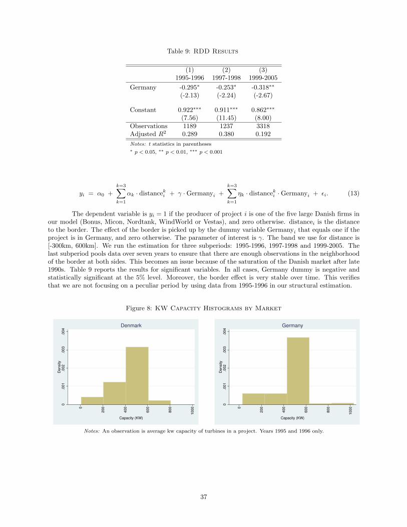
Table 9: RDD Results

(1) (2) (3)1995-1996 1997-1998 1999-2005

Germany -0.295∗ -0.253∗ -0.318∗∗

(-2.13) (-2.24) (-2.67)

Constant 0.922∗∗∗ 0.911∗∗∗ 0.862∗∗∗

(7.56) (11.45) (8.00)Observations 1189 1237 3318Adjusted R2 0.289 0.380 0.192

Notes: t statistics in parentheses∗ p < 0.05, ∗∗ p < 0.01, ∗∗∗ p < 0.001

yi = α0 +

k=3∑k=1

αk · distanceki + γ ·Germanyi +

k=3∑k=1

ηk · distanceki ·Germanyi + εi. (13)

The dependent variable is yi = 1 if the producer of project i is one of the five large Danish firms inour model (Bonus, Micon, Nordtank, WindWorld or Vestas), and zero otherwise. distancei is the distanceto the border. The effect of the border is picked up by the dummy variable Germanyi that equals one if theproject is in Germany, and zero otherwise. The parameter of interest is γ. The band we use for distance is[-300km, 600km]. We run the estimation for three subperiods: 1995-1996, 1997-1998 and 1999-2005. Thelast subperiod pools data over seven years to ensure that there are enough observations in the neighborhoodof the border at both sides. This becomes an issue because of the saturation of the Danish market after late1990s. Table 9 reports the results for significant variables. In all cases, Germany dummy is negative andstatistically significant at the 5% level. Moreover, the border effect is very stable over time. This verifiesthat we are not focusing on a peculiar period by using data from 1995-1996 in our structural estimation.

Figure 8: KW Capacity Histograms by Market

0.0

01

.002

.003

.004

Density

0

200

400

600

800

1000

Capacity (KW)

Denmark

0.0

01

.002

.003

.004

Density

0

200

400

600

800

1000

Capacity (KW)

Germany

Notes: An observation is average kw capacity of turbines in a project. Years 1995 and 1996 only.

37

Figure 9: Tower Height Histograms by Producer and Market

0.0

2.0

4.0

6.0

80

.02

.04

.06

.08

0.0

2.0

4.0

6.0

8

0

10

20

30

40

50

60

70 0

10

20

30

40

50

60

70 0

10

20

30

40

50

60

70 0

10

20

30

40

50

60

70

Bonus in DNK Bonus in GER Micon in DNK Micon in GER

Nordex in DNK Nordex in GER Nordtank in DNK Nordtank in GER

Vestas in DNK Vestas in GER Wind World in DNK Wind World in GER

Density

Tower Height (m)

Notes: An observation is average tower height of turbines in a project. Years 1995 and 1996 only. “Bonus in DNK (GER)”indicates projects supplied by Bonus in Denmark (Germany).

Figure 10: KW Capacity Histograms by Producer and Market

0

.001

.002

.003

.004

.005

0

.001

.002

.003

.004

.005

0

.001

.002

.003

.004

.005

0

200

400

600

800

1000 0

200

400

600

800

1000 0

200

400

600

800

1000 0

200

400

600

800

1000

Bonus in DNK Bonus in GER Micon in DNK Micon in GER

Nordex in DNK Nordex in GER Nordtank in DNK Nordtank in GER

Vestas in DNK Vestas in GER Wind World in DNK Wind World in GER

Density

Capacity (KW)

Notes: An observation is average kw capacity of turbines in a project. Years 1995 and 1996 only. “Bonus in DNK (GER)”indicates projects supplied by Bonus in Denmark (Germany).

38

Figure 11: Per KW List Prices of Various Turbines Offered in 1995-1996

1

1.5

2

2.5

3

3.5

4

4.5

5

Price/K

W (

1000 D

euts

che M

ark

in 1

994 p

rices)

0 100 200 300 400 500 600 700 800 900 1000

Capacity (KW)

Notes: Pooled over all producers.

Appendix B Robustness to Local Unobservables and Economiesof Density

In order to derive the pricing equation, our model assumes that the unobservable shock to managers profits,ε`ij , is unknown to firms, but drawn from a known distribution which is independent across projects andfirms. Thus, we abstract away from the existence of spatial autocorrelation of unobservables across projects.This section assesses whether this assumption has the potential to bias our estimate of the border effect.

There are several reasons for being concerned about the independence assumption. The assumptionwill be violated if firms directly observe sources of firm-project cost variation which are not explicitly con-trolled for by the model. While we feel that firms’ productivity levels, firm-project distances, and the borderdummy are the primary determinants of costs, other potential sources of variation could relate to unobserv-able local conditions being more amenable to a particular firm (e.g., local politics or geographic featuresof an area could result in lower cost for some firms). The independence assumption will also be violatedif economies of density can be realized by a firm constructing several projects located geographically closetogether. Economies of density might be present if, for example, clustering projects together reduces travelcosts for routine maintenance. Such economies of density might make the individual projects less expensiveto maintain on a per-unit basis, leading firms with nearby installed projects to have a cost advantage overother firms that is not recognized in our model.

The existence of local unobservables would generate spatial autocorrelation in the error terms be-tween projects which are geographically close. This would violate our assumption that the errors are inde-pendent across projects. Moreover, if firms are responding to economies of density of projects, firms pricingdecisions become dynamic in nature. Since winning a project today lowers the firms’ costs on other projectsin the future, firms would not choose prices to maximize project-level profits, but rather the present dis-counted value of profits on this project and future projects. Both of these forces would lead firm’s projects tobe more tightly clustered together than our model would predict, leading to spatial autocorrelation in firms’error terms across projects. To test for the presence of spatial autocorrelation, we consider the followingparametric model for the error term,

39

εj = γ + ψWεj + νi. (14)

Here, εj is the vector of private shocks for firm j in all projects, γ is Euler’s constant—the mean ofthe extreme value distribution, W is a known spatial weight matrix that determines the degree of influenceone project has on another, and νi are independent and identically distributed mean-zero shocks. Thescalar ψ determines the degree of spatial autocorrelation, we wish to test the null hypothesis that spatialautocorrelation is not present, i.e., that ψ = 0 and the εij are in fact independent across projects.

In order to perform the test, we must specify the spatial weight matrix W . An element of the spatialweight matrix, Wik provides an indication of how strongly project k is related to project i. Clearly manydifferent specifications are possible, including inverse distance (measured either directly or though a roadnetwork), inclusion within the same region, or nearest neighbor adjacency. In practice we specify W as,

Wik =

{1 if dist(i, k) < 30km,

0 otherwise,

where distance is the direct distance (as the crow flies) in kilometers between projects i and j.40

We are unable to directly test for spatial autocorrelation in ε`ij because as with all discrete choice

models, ε`ij is not directly recoverable. Instead, we follow Pinkse and Slade (1998) and test our results

for spatial autocorrelation using the generalized errors. The generalized errors are the expectation of ε`ijconditioned on the observed data and the model being correctly specified. Given the structure of our model,the generalized errors can be derived using the extreme-value density function,41

ε`ij =

γ − log ρ`ij if y`ij = 1,

γ +ρ`ij

1−ρ`ijlog ρ`ij if y`ij = 0.

Again γ, represents Euler’s constant—the unconditional expectation of the extreme value distribution. Whilethe derivation of these expectations is algebraically tedious, the result is intuitive: the more likely a man-ufacturer j is to be selected by the project manager, the lower ε`ij must be in order for selection to occur.

Hence, ε`ij is decreasing in the ex-ante probability of firm j being selected. The fact that the distribution

of ε`ij conditional on j not being chosen is independent of the actual choice observed in market i is a con-sequence of the well known independence of irrelevant alternatives (IIA) property of extreme-value discretechoice models. Note that, if the null hypothesis of no auto-correlation is violated, ε`ij will be mis-specified.Nonetheless, they are useful to conduct a hypothesis test that ψ = 0.

We can use ordinary least squares to estimate ψ from the equation,

εj = γ + ψWεj + νi

and test whether ψ = 0. Note that, the estimate we generate, ψ, is only consistent under the null hypothesissince the null is assumed in the construction of εj and ordinary least squares is only consistent if ψ = 0.

The results are reported in Table 10.42 While the magnitude of the estimated ψ is small, the teststrongly rejects the null hypothesis for every firm, due in part to the the high precision of the estimates. Weconclude that some degree of spatial autocorrelation is present, although it appears to be mild.

The presence of spatial autocorrelation has the potential to bias our estimate of the border effect. Inparticular, if spatial autocorrelation is due to cost or demand advantages in installing near already completedprojects constructed by the same manufacturer, and if exporters have a smaller installed base within a countrythan do domestic firms, then the border effect may be capturing differences in the installed bases of foreignand domestic firms in addition to the variable cost of exporting. Alternatively, if serial correlation is due tolocal unobserved characteristics then the location of previous installations, while not cost reducing in and

40Our results are robust to raising or lowering the distance cutoff and using a specification of W based on inverse distance.41The derivation is available from the authors upon request.42It is important that the test be conducted with heteroskedasticity-robust variance estimates, since there is little reason to

believe that the generalized errors are homoscedastic.

40

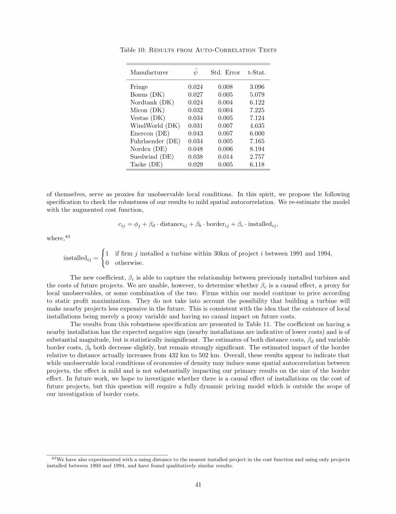
Table 10: Results from Auto-Correlation Tests

Manufacturer ψ Std. Error t-Stat.

Fringe 0.024 0.008 3.096Bonus (DK) 0.027 0.005 5.079Nordtank (DK) 0.024 0.004 6.122Micon (DK) 0.032 0.004 7.225Vestas (DK) 0.034 0.005 7.124WindWorld (DK) 0.031 0.007 4.635Enercon (DE) 0.043 0.007 6.000Fuhrlaender (DE) 0.034 0.005 7.165Nordex (DE) 0.048 0.006 8.194Suedwind (DE) 0.038 0.014 2.757Tacke (DE) 0.029 0.005 6.118

of themselves, serve as proxies for unobservable local conditions. In this spirit, we propose the followingspecification to check the robustness of our results to mild spatial autocorrelation. We re-estimate the modelwith the augmented cost function,

cij = φj + βd · distanceij + βb · borderij + βc · installedij ,

where,43

installedij =

{1 if firm j installed a turbine within 30km of project i between 1991 and 1994,

0 otherwise.

The new coefficient, βc is able to capture the relationship between previously installed turbines andthe costs of future projects. We are unable, however, to determine whether βc is a causal effect, a proxy forlocal unobservables, or some combination of the two. Firms within our model continue to price accordingto static profit maximization. They do not take into account the possibility that building a turbine willmake nearby projects less expensive in the future. This is consistent with the idea that the existence of localinstallations being merely a proxy variable and having no causal impact on future costs.

The results from this robustness specification are presented in Table 11. The coefficient on having anearby installation has the expected negative sign (nearby installations are indicative of lower costs) and is ofsubstantial magnitude, but is statistically insignificant. The estimates of both distance costs, βd and variableborder costs, βb both decrease slightly, but remain strongly significant. The estimated impact of the borderrelative to distance actually increases from 432 km to 502 km. Overall, these results appear to indicate thatwhile unobservable local conditions of economies of density may induce some spatial autocorrelation betweenprojects, the effect is mild and is not substantially impacting our primary results on the size of the bordereffect. In future work, we hope to investigate whether there is a causal effect of installations on the cost offuture projects, but this question will require a fully dynamic pricing model which is outside the scope ofour investigation of border costs.

43We have also experimented with a using distance to the nearest installed project in the cost function and using only projectsinstalled between 1993 and 1994, and have found qualitatively similar results.

41

Table 11: Robustness Check: Nearby Installed Turbines

Coefficient Std. Error

Border Variable Cost, βb 0.688 (0.178)Distance Cost (100km), βd 0.137 (0.031)Nearby Installation, βc -1.249 (1.167)

Firm Fixed Effects, ξjBonus (DK) 1.256 (0.189)Nordtank (DK) 1.462 (0.183)Micon (DK) 2.046 (0.160)Vestas (DK) 2.689 (0.170)WindWorld (DK) 0.640 (0.211)Enercon (DE) 2.719 (0.147)Fuhrlaender (DE) -0.010 (0.266)Nordex (DE) 0.858 (0.184)Suedwind (DE) -0.187 (0.206)Tacke (DE) 1.578 (0.152)

Log-Likelihood -2286.15N 1226

Appendix C Computational Method

C.1 Estimation of the Project Bidding Game

We formulate the estimation of the project bidding game as a constrained optimization problem.44 The objec-tive is to maximize the likelihood function subject to satisfying the firm-project specific winning probabilitiesexpressions that come out of our model. We reformulate the problem defined in (10) for the computationalimplementation. The reformulated constraints are mathematically equivalent to those in (10). They comewith two major advantages: First, when we reformulate the system maximizing the log-likelihood insteadof the likelihood function, and rewrite the constraints, we are removing most of the nonlinearity. Second,winning probabilities only affect their respective equation and the adding-up constraint for the respectiveproject. The sparse structure of the Jacobian of the constraints makes this large optimization problemfeasible. The reformulated problem is

maxθ, ρ

∑`∈{D,G}

N∑i=1

|J`|∑j=1

y`ij log ρ`ij

subject to: log ρ`ij − log ρ`i0 = ξj − βd · distanceij − βb · border`ij −1

1− ρ`ij|J`|∑k=1

ρ`ik + ρ`i0 = 1

for ` ∈ {D,G}, i ∈ {1, ..., N`}, j ∈ J .

For the baseline estimation, there are 11 constraints for every German project, and 7 constraintsfor every Danish project (|JG| = 10 and |JD| = 6 plus one fringe firm in every market). Since we have 930

44See Judd and Su (2011) for a seminal paper that explains why constrained optimization of structural models is oftensuperior to estimation via nested fixed points.

42

German and 296 Danish project this aggregates to 12,302 constraints. In our baseline specification we arechoosing 12,314 variables (12 structural parameters and 12,302 equilibrium win probabilities for each firmin each market)

We use the constrained optimization solver KNITRO to solve the problem. To improve speedand accuracy of the estimation, we hand-code the analytical derivatives of the object of function and theconstraints and provide the sparsity structure of the Jacobian to the solver.45 In order to find a globalmaximum we pick 10 random starting values for the structural parameters. The estimation converges to thesame solution for all attempted starting values.

We calculate the covariance matrix of the parameter estimates using the outer product rule.1. First, we calculate the score of each winning firm project pair, ∂ log ρ∗i /∂θ, using numerical

derivatives. This involves perturbing the θ vector. Note that the step size to perturb θ should be larger thanthe numerical tolerance level of the equilibrium constraints. Then the equilibrium constraints are resolved.

2. We then calculate the inverse of the covariance matrix:

S(θ) =

N∑i=1

∂ log ρ∗i (θ)

∂θ

∂ log ρ∗i (θ)

∂θ

′

C.2 Counterfactuals

The point estimate θ automatically satisfies the equilibrium constraints in the benchmark scenario withfixed entry and variable border costs. In the counterfactual “No fixed border costs” we use θ to thenresolve the equilibrium constraints, with every firm being active in every market, |JD| = |JG| = 10. In thecounterfactual “No border costs” we resolve the same system of equilibrium constraints with the variableborder cost coefficient set to zero.

We use a parametric bootstrap procedure to calculate the standard errors for our counterfactuals. Wedraw 200 parameter vectors from the distribution of estimated parameters (multivariate normal distribution

with mean θ and covariance matrix S(θ)−1). First we resolve the baseline equilibrium constraints, then theconstraints for the scenario with no fixed entry costs, and finally the constraints for the no border costsscenario (with each firm active in every market and the variable border costs coefficient set to zero). Westore the equilibrium outcomes from each of these draws and use them to calculate the standard errors forour counterfactuals.

45Prior to the estimation we check via finite differences that our analytical gradients are correct.

43