


Languages
Pages
Legal


CONFIDENTIAL
This report is solely for the use of client personnel. No part of it may be circulated, quoted, or reproduced for distribution outside the client organization without prior written approval from McKinsey & Company. This material was used by McKinsey & Company during an oral presentation; it is not a complete record of the discussion.
DocumentDate
Excel Tips That Could Save You from Working All Night
* FootnoteSource: Sources
Unit of measuresSTICKER
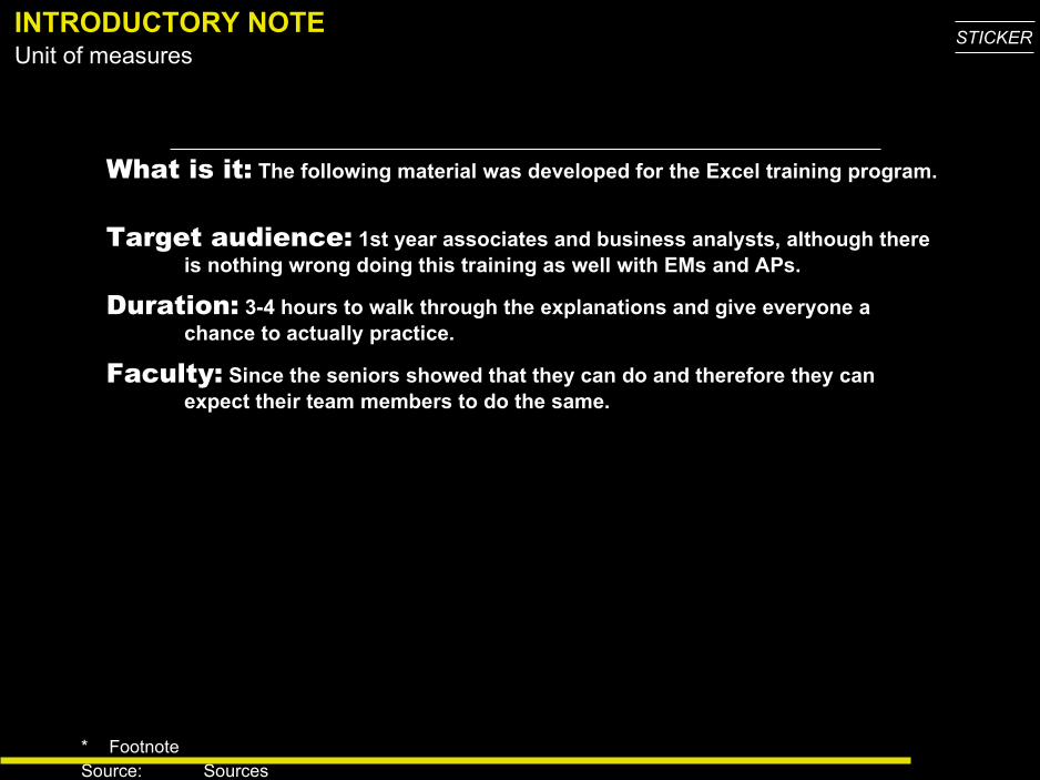
What is it: The following material was developed for the Excel training program.
Target audience: 1st year associates and business analysts, although there is nothing wrong doing this training as well with EMs and APs.
Duration: 3-4 hours to walk through the explanations and give everyone a chance to actually practice.
Faculty: Since the seniors showed that they can do and therefore they can expect their team members to do the same.
INTRODUCTORY NOTE
* FootnoteSource: Sources
Unit of measuresSTICKER
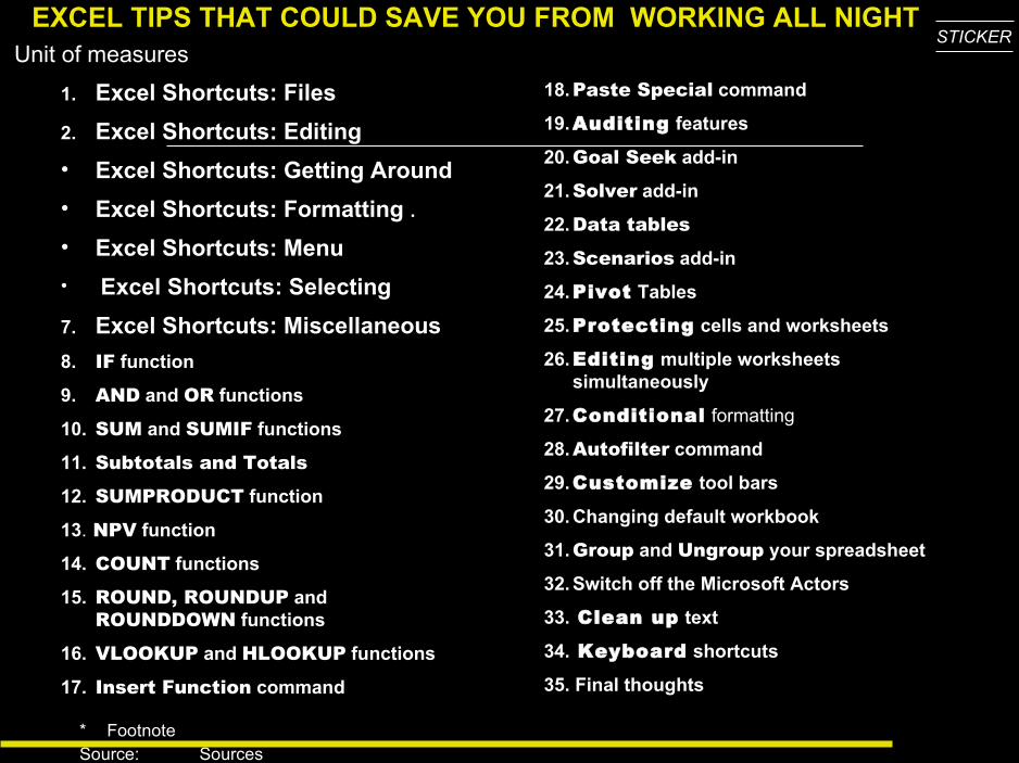
1. Excel Shortcuts: Files
2. Excel Shortcuts: Editing
• Excel Shortcuts: Getting Around
• Excel Shortcuts: Formatting .
• Excel Shortcuts: Menu
• Excel Shortcuts: Selecting
7. Excel Shortcuts: Miscellaneous
8. IF function
9. AND and OR functions
10. SUM and SUMIF functions
11. Subtotals and Totals
12. SUMPRODUCT function
13. NPV function
14. COUNT functions
15. ROUND, ROUNDUP and ROUNDDOWN functions
16. VLOOKUP and HLOOKUP functions
17. Insert Function command
18.Paste Special command
19.Auditing features
20.Goal Seek add-in
21.Solver add-in
22.Data tables
23.Scenarios add-in
24.Pivot Tables
25.Protecting cells and worksheets
26.Editing multiple worksheets simultaneously
27.Conditional formatting
28.Autofilter command
29.Customize tool bars
30. Changing default workbook
31.Group and Ungroup your spreadsheet
32. Switch off the Microsoft Actors
33. Clean up text
34. Keyboard shortcuts
35. Final thoughts
EXCEL TIPS THAT COULD SAVE YOU FROM WORKING ALL NIGHT

* FootnoteSource: Sources
Unit of measuresSTICKER
•This small group of shortcuts is useful for opening, closing and saving your Excel workbooks.
How you use this feature
•Ctrl+S: Save your Excel workbook •Ctrl+O: Open an existing Excel workbook •Ctrl+N: Create a new Excel workbook
Exercise
•Open a new file Excel workbook and save it.
1. Excel Shortcuts: Files
zWhy you need to do this
* FootnoteSource: Sources
Unit of measuresSTICKER
•These are common shortcuts you will use to edit your Excel workbook. Our favorite shortcut in this list is, quite obviously, Ctrl+Z.
– Ctrl+C: Copy the current selection to the clipboard. After you copy something, you can paste it with the paste shortcut.
– Ctrl+V: Paste the current item from the clipboard.
– Ctrl+X: Cut the current selection and place it on the clipboard, which can be pasted. The difference between cut and copy is that cut will delete your selection, while copy will not.
– Ctrl+Z: Undo your last change. This is can be repeated to remove again and again to undo many changes.
– Ctrl+Y: Redo your last Undo. This only is available if you have just issued an Undo command.
Excel Shortcuts: Editing
How you use this feature
Why you need to know this
* FootnoteSource: Sources
Unit of measuresSTICKER
•These shortcuts will help you move around your Excel workbooks and worksheets with great ease!
•Page Up: Move one page up in your worksheet •Page Down: Move one page down in your worksheet.
Note: The number of rows moved in both page up and page down depend on how many rows are currently displayed. The more rows you have displayed the greater amount the row jump will be when you do a page up/down.
•Ctrl+Home: Move to the beginning of your worksheet •Ctrl+End: Move to the end of your worksheet •Tab: Move right one column •Shift+Tab: Move left one column •Ctrl+Page Up: Go back one worksheet•Ctrl+Page Down: Go forward one worksheet. Note: If you
are not using multiple worksheets in your workbook you will probably not use this shortcut!
Excel Shortcuts: Getting Around
How you use this feature
Why you need to know this
* FootnoteSource: Sources
Unit of measuresSTICKER
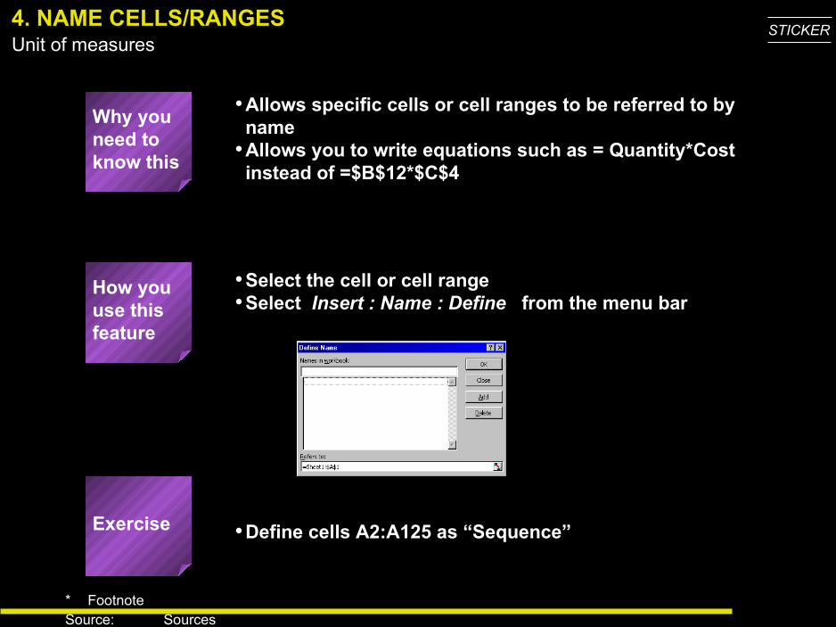
•Allows specific cells or cell ranges to be referred to by name
•Allows you to write equations such as = Quantity*Cost instead of =$B$12*$C$4
•Select the cell or cell range•Select Insert : Name : Define from the menu bar
•Define cells A2:A125 as “Sequence”
4. NAME CELLS/RANGES
How you use this feature
Exercise
Why you need to know this
* FootnoteSource: Sources
Unit of measuresSTICKER
•Correctly sorting a series of rows or columns without disassociating the data is critical to many modeling efforts
5. SORT COMMAND
How you use this feature
Why you need to know this
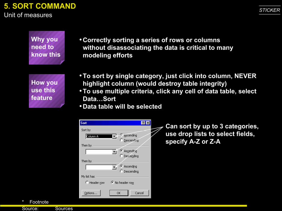
•To sort by single category, just click into column, NEVER highlight column (would destroy table integrity)
•To use multiple criteria, click any cell of data table, select Data…Sort
•Data table will be selected
Can sort by up to 3 categories, use drop lists to select fields, specify A-Z or Z-A
* FootnoteSource: Sources
Unit of measuresSTICKER
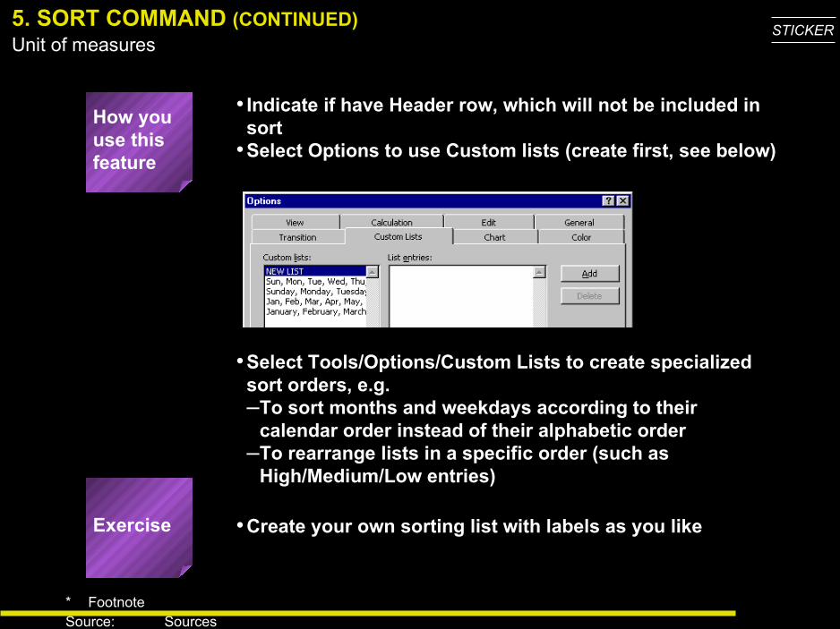
•Select Tools/Options/Custom Lists to create specialized sort orders, e.g.–To sort months and weekdays according to their
calendar order instead of their alphabetic order –To rearrange lists in a specific order (such as
High/Medium/Low entries)
Exercise
• Indicate if have Header row, which will not be included in sort
•Select Options to use Custom lists (create first, see below)
How you use this feature
5. SORT COMMAND (CONTINUED)
•Create your own sorting list with labels as you like
* FootnoteSource: Sources
Unit of measuresSTICKER
•Saves you lots of time
•F4 key toggles through the different options
6. TOGGLING AMONG RELATIONAL AND ABSOLUTE REFERENCES
How you use this feature
Why you need to know this
* FootnoteSource: Sources
Unit of measuresSTICKER
•Saves you lots of time•Allows for copying of cell content to contiguous cells
with a single keystroke
•Select the cell with the content to be copied and drag to select the cells to which the content should be copied
•Ctrl-R to fill right•Ctrl-D to fill down
•Double-check your formulas for absolute vs. relative references!!
•Calculate the total daily sales for each store
How you use this feature
Exercise
Caution!!
7. FILL DOWN AND FILL RIGHT COMMANDS
Why you need to know this
* FootnoteSource: Sources
Unit of measuresSTICKER
•Conditional comparisons are used in virtually all spreadsheets
•Knowing how to use IF in a nested manner and in combination with other functions will save hours of time
• IF(Comparison,TrueAction,FalseAction)• IF(Comparison,TrueAction,) ==> Cell shows 0 if
condition is false• IF(Comparison,TrueAction,””) ==> Cell shows blank if
condition is false
•Create a “Mumbai” variable–1 if the store is in Mumbai–0 if the store is in other places
8. IF FUNCTION
How you use this feature
Exercise
Why you need to know this
* FootnoteSource: Sources
Unit of measuresSTICKER
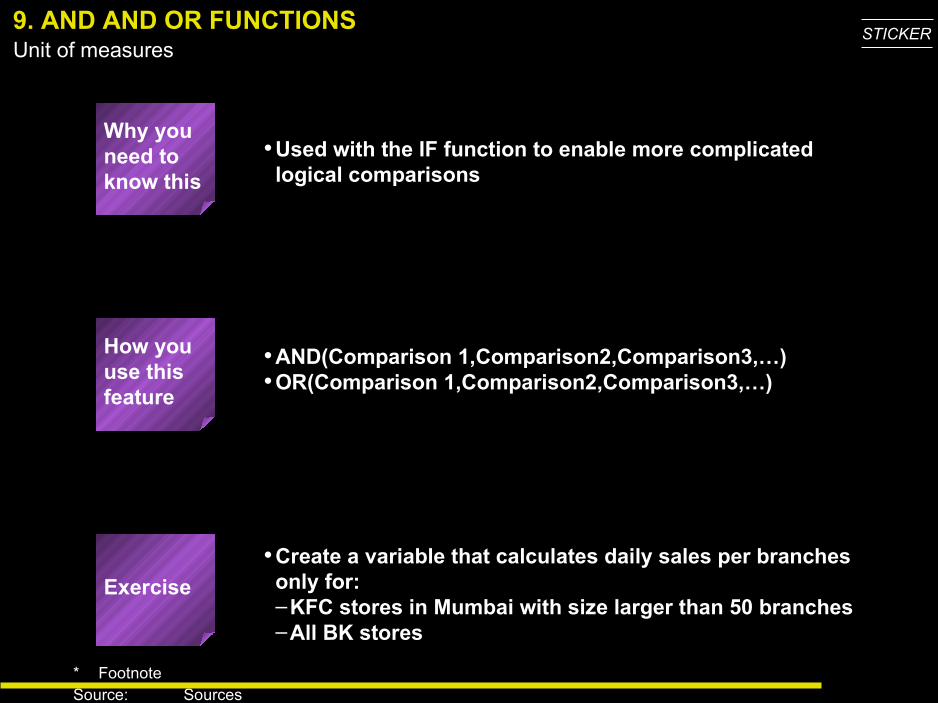
•Used with the IF function to enable more complicated logical comparisons
•AND(Comparison 1,Comparison2,Comparison3,…)•OR(Comparison 1,Comparison2,Comparison3,…)
•Create a variable that calculates daily sales per branches only for:–KFC stores in Mumbai with size larger than 50 branches–All BK stores
9. AND AND OR FUNCTIONS
How you use this feature
Exercise
Why you need to know this
* FootnoteSource: Sources
Unit of measuresSTICKER
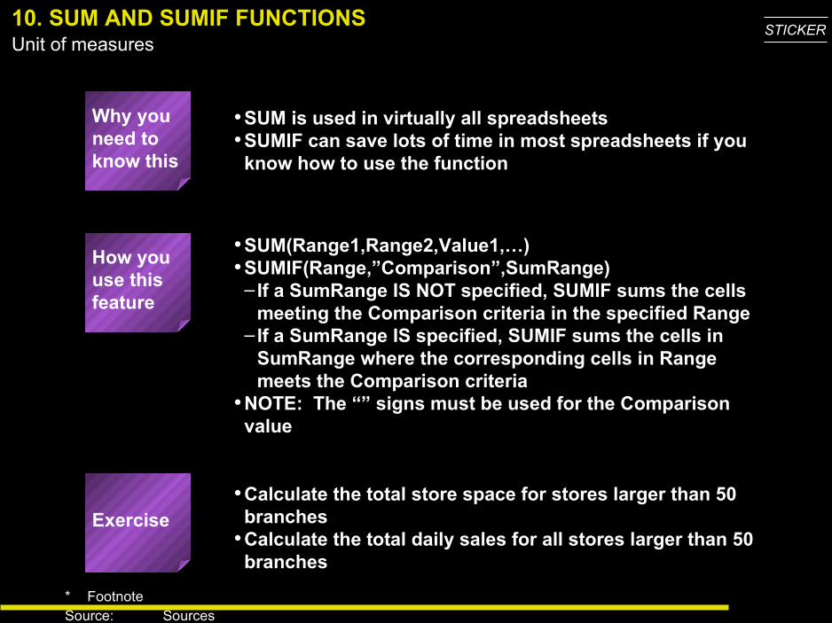
•SUM is used in virtually all spreadsheets•SUMIF can save lots of time in most spreadsheets if you
know how to use the function
•SUM(Range1,Range2,Value1,…)•SUMIF(Range,”Comparison”,SumRange)
– If a SumRange IS NOT specified, SUMIF sums the cells meeting the Comparison criteria in the specified Range
– If a SumRange IS specified, SUMIF sums the cells in SumRange where the corresponding cells in Range meets the Comparison criteria
•NOTE: The “” signs must be used for the Comparison value
•Calculate the total store space for stores larger than 50 branches
•Calculate the total daily sales for all stores larger than 50 branches
10. SUM AND SUMIF FUNCTIONS
How you use this feature
Exercise
Why you need to know this
* FootnoteSource: Sources
Unit of measuresSTICKER
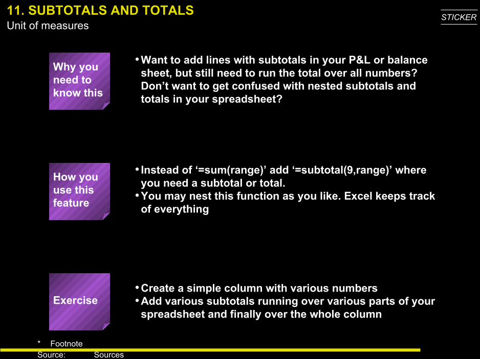
•Want to add lines with subtotals in your P&L or balance sheet, but still need to run the total over all numbers? Don’t want to get confused with nested subtotals and totals in your spreadsheet?
• Instead of ‘=sum(range)’ add ‘=subtotal(9,range)’ where you need a subtotal or total.
•You may nest this function as you like. Excel keeps track of everything
•Create a simple column with various numbers•Add various subtotals running over various parts of your
spreadsheet and finally over the whole columnExercise
How you use this feature
11. SUBTOTALS AND TOTALS
Why you need to know this
* FootnoteSource: Sources
Unit of measuresSTICKER
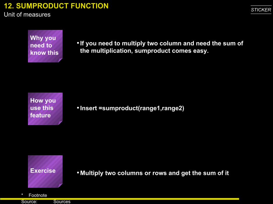
• If you need to multiply two column and need the sum of the multiplication, sumproduct comes easy.
• Insert =sumproduct(range1,range2)
•Multiply two columns or rows and get the sum of it
12. SUMPRODUCT FUNCTION
Exercise
How you use this feature
Why you need to know this
* FootnoteSource: Sources
Unit of measuresSTICKER
•Of course you can create your own discounting table and then calculate the NPV of your cash flow series or just use the NPV function
• Insert =NPV(discount rate,cash flow numbers,...)•The discount rate is in percent•The cash flow numbers are either an array or individual
numbers in individual cells•Attention: The first cash flow number is in period 1, e.g.
the end of the period. If you have for example an initial investment in period 0, just type =NPV(…)+period 0 payment in your calculation
•Create a list of random cash flows and calculate the NPV with the NPV function
13. NPV FUNCTION
Exercise
How you use this feature
Why you need to know this
* FootnoteSource: Sources
Unit of measuresSTICKER
•Prevents you from wasting time counting items manually or creating dummy variables to count such items
•COUNT(Range1,Range2,Value1,...) ==> count the number of cells containing numbers
•COUNTA(Range1,Range2,Value1,...) ==> count the number of non-empty cells
•COUNTBLANK(Range) ==> count the number of empty cells in the range
•COUNTIF(Range,”Criteria”) ==> count the number of cells in the Range containing the Criteria. NOTE: The “” signs must be used for the Criteria value
•Calculate the number of KFC stores in the dataset
14. COUNT FUNCTIONS
How you use this feature
Exercise
Why you need to know this
* FootnoteSource: Sources
Unit of measuresSTICKER
•Many situations exist when you need to have exact numbers instead of various fractions in your calculations (e.g., there cannot be 536.235 bank branches)
•ROUND(Number,Digits) ==> Round the number (or cell) to the specified number of digits– If Digit = 0, then Number is rounded to nearest integer– If Digit > 0, then Number is rounded to the specified
number of decimal places– If Digit < 0, then Number is rounded to the specified
number of digits left of the decimal place•ROUNDDOWN(Number,Digits) and
ROUNDUP(Number,Digits) work the same way as ROUND, but the direction of rounding is specified by the function
•Calculate a rounded Avg Sale/Ticket variable, rounding to the nearest 10 Won
15. ROUND, ROUNDUP AND ROUNDDOWN FUNCTIONS
How you use this feature
Exercise
Why you need to know this
* FootnoteSource: Sources
Unit of measuresSTICKER
•Allows you to automatically lookup a particular cell of data from a larger data range. This is especially useful when you have–A large data section that contains information for
multiple records somewhere on the spreadsheet (e.g., a small database)
–A calculation area somewhere else, and you need to refer to some specific data elements for specific records
16. VLOOKUP AND HLOOKUP FUNCTIONS
Why you need to know this
* FootnoteSource: Sources
Unit of measuresSTICKER
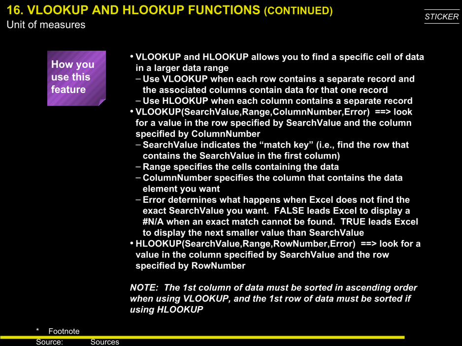
• VLOOKUP and HLOOKUP allows you to find a specific cell of data in a larger data range– Use VLOOKUP when each row contains a separate record and
the associated columns contain data for that one record– Use HLOOKUP when each column contains a separate record
• VLOOKUP(SearchValue,Range,ColumnNumber,Error) ==> look for a value in the row specified by SearchValue and the column specified by ColumnNumber– SearchValue indicates the “match key” (i.e., find the row that
contains the SearchValue in the first column)– Range specifies the cells containing the data– ColumnNumber specifies the column that contains the data
element you want– Error determines what happens when Excel does not find the
exact SearchValue you want. FALSE leads Excel to display a #N/A when an exact match cannot be found. TRUE leads Excel to display the next smaller value than SearchValue
• HLOOKUP(SearchValue,Range,RowNumber,Error) ==> look for a value in the column specified by SearchValue and the row specified by RowNumber
NOTE: The 1st column of data must be sorted in ascending order when using VLOOKUP, and the 1st row of data must be sorted if using HLOOKUP
16. VLOOKUP AND HLOOKUP FUNCTIONS (CONTINUED)
How you use this feature
* FootnoteSource: Sources
Unit of measuresSTICKER
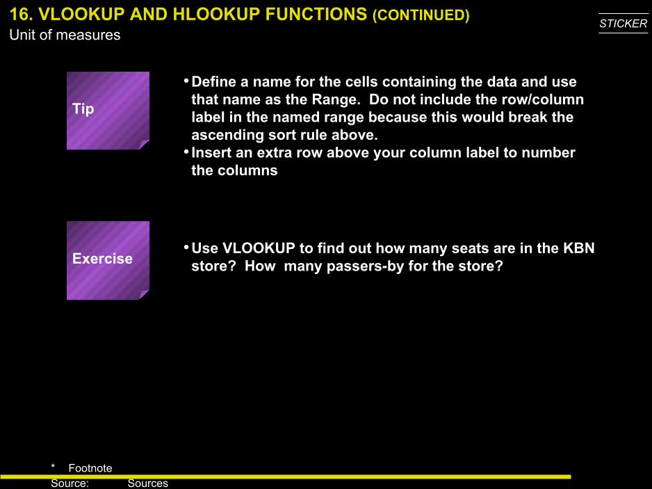
•Define a name for the cells containing the data and use that name as the Range. Do not include the row/column label in the named range because this would break the ascending sort rule above.
• Insert an extra row above your column label to number the columns
•Use VLOOKUP to find out how many seats are in the KBN store? How many passers-by for the store?
16. VLOOKUP AND HLOOKUP FUNCTIONS (CONTINUED)
Exercise
Tip
* FootnoteSource: Sources
Unit of measuresSTICKER
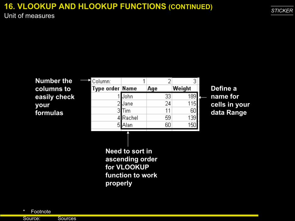
Define a name for cells in your data Range
Number the columns to easily check your formulas
Need to sort in ascending order for VLOOKUP function to work properly
16. VLOOKUP AND HLOOKUP FUNCTIONS (CONTINUED)
* FootnoteSource: Sources
Unit of measuresSTICKER
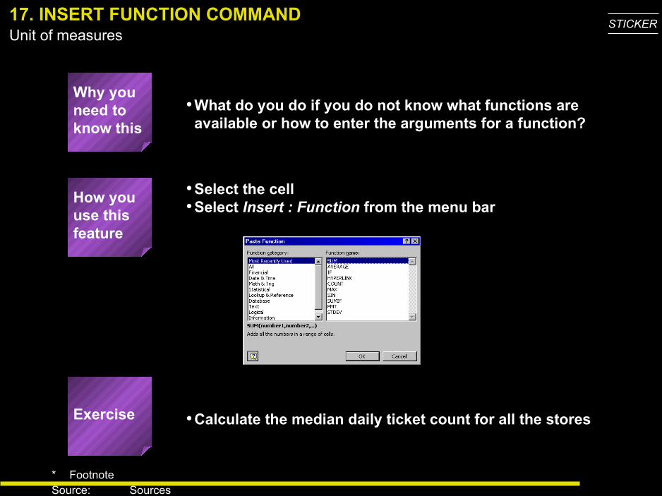
•What do you do if you do not know what functions are available or how to enter the arguments for a function?
•Select the cell•Select Insert : Function from the menu bar
•Calculate the median daily ticket count for all the stores
17. INSERT FUNCTION COMMAND
How you use this feature
Exercise
Why you need to know this
* FootnoteSource: Sources
Unit of measuresSTICKER
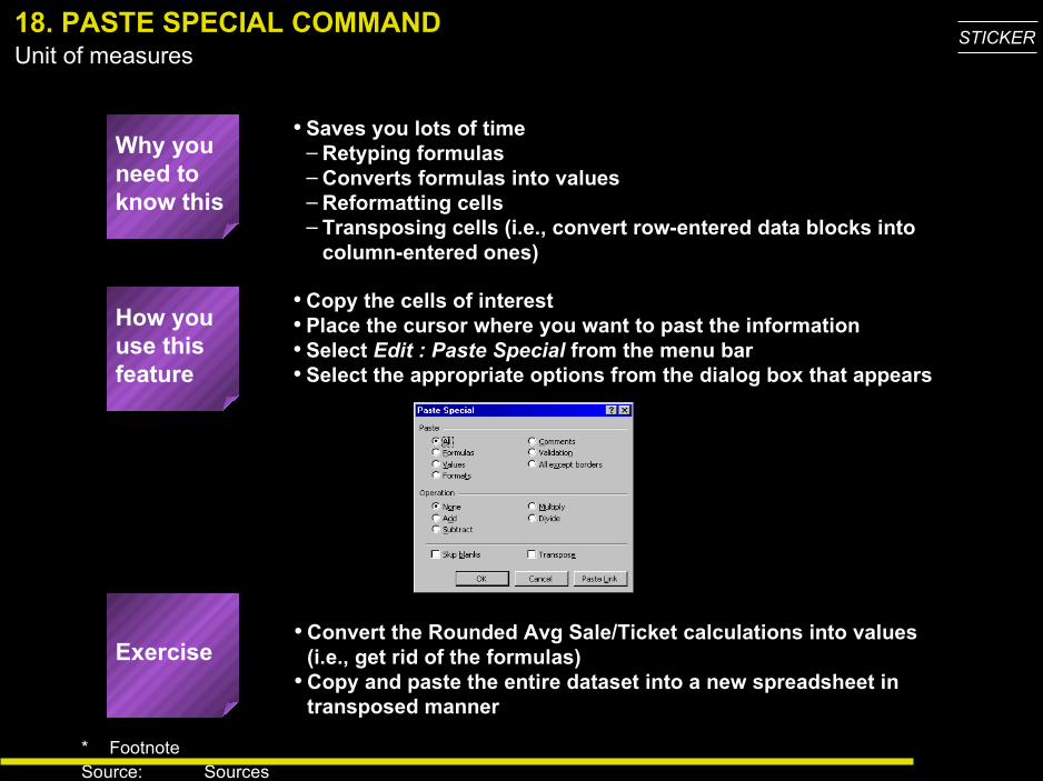
• Saves you lots of time– Retyping formulas– Converts formulas into values– Reformatting cells– Transposing cells (i.e., convert row-entered data blocks into
column-entered ones)
• Convert the Rounded Avg Sale/Ticket calculations into values (i.e., get rid of the formulas)
• Copy and paste the entire dataset into a new spreadsheet in transposed manner
• Copy the cells of interest• Place the cursor where you want to past the information• Select Edit : Paste Special from the menu bar• Select the appropriate options from the dialog box that appears
18. PASTE SPECIAL COMMAND
How you use this feature
Exercise
Why you need to know this
* FootnoteSource: Sources
Unit of measuresSTICKER
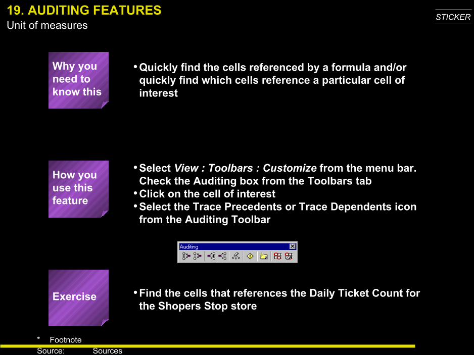
•Quickly find the cells referenced by a formula and/or quickly find which cells reference a particular cell of interest
•Select View : Toolbars : Customize from the menu bar. Check the Auditing box from the Toolbars tab
•Click on the cell of interest•Select the Trace Precedents or Trace Dependents icon
from the Auditing Toolbar
•Find the cells that references the Daily Ticket Count for the Shopers Stop store
19. AUDITING FEATURES
How you use this feature
Exercise
Why you need to know this
* FootnoteSource: Sources
Unit of measuresSTICKER
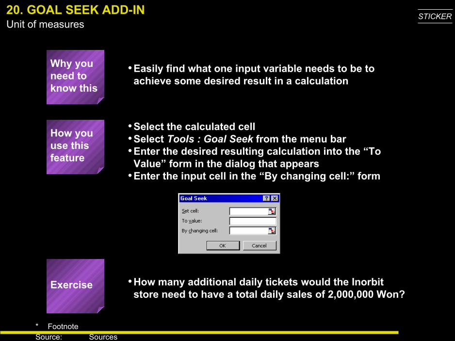
•Easily find what one input variable needs to be to achieve some desired result in a calculation
•Select the calculated cell•Select Tools : Goal Seek from the menu bar•Enter the desired resulting calculation into the “To
Value” form in the dialog that appears•Enter the input cell in the “By changing cell:” form
•How many additional daily tickets would the Inorbit store need to have a total daily sales of 2,000,000 Won?
20. GOAL SEEK ADD-IN
How you use this feature
Exercise
Why you need to know this
* FootnoteSource: Sources
Unit of measuresSTICKER
•Allows you to use linear programming to find the optimal inputs to achieve some desired calculational result (e.g., maximize revenues by increasing daily tickets, increasing store size, average sale/ticket, etc. simultaneously)
•Use Solver instead of Goal Seek when:–You need to place constraints on the input variable
(e.g., cannot open a store for more than 24 hours a day)–More than 1 input variables are involved–You want to minimize or maximize the resulting
calculation in addition to just setting the calculation to a predetermined value
21. SOLVER ADD-IN
Why you need to know this
* FootnoteSource: Sources
Unit of measuresSTICKER
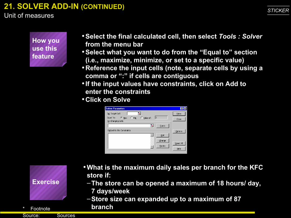
•Select the final calculated cell, then select Tools : Solver from the menu bar
•Select what you want to do from the “Equal to” section (i.e., maximize, minimize, or set to a specific value)
•Reference the input cells (note, separate cells by using a comma or “:” if cells are contiguous
• If the input values have constraints, click on Add to enter the constraints
•Click on Solve
•What is the maximum daily sales per branch for the KFC store if:–The store can be opened a maximum of 18 hours/ day,
7 days/week–Store size can expanded up to a maximum of 87
branch
How you use this feature
Exercise
21. SOLVER ADD-IN (CONTINUED)
* FootnoteSource: Sources
Unit of measuresSTICKER
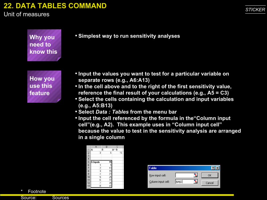
• Simplest way to run sensitivity analyses
• Input the values you want to test for a particular variable on separate rows (e.g., A6:A13)
• In the cell above and to the right of the first sensitivity value, reference the final result of your calculations (e.g., A5 = C3)
• Select the cells containing the calculation and input variables (e.g., A5:B13)
• Select Data : Tables from the menu bar• Input the cell referenced by the formula in the“Column input
cell”(e.g., A2). This example uses in “Column input cell” because the value to test in the sensitivity analysis are arranged in a single column
22. DATA TABLES COMMAND
How you use this feature
Why you need to know this
* FootnoteSource: Sources
Unit of measuresSTICKER
•What daily total sales would the KFC store have its daily ticket counts ranged from 400 to 600 each day (in increments of 50)?
22. DATA TABLES COMMAND (CONTINUED)
Exercise
* FootnoteSource: Sources
Unit of measuresSTICKER
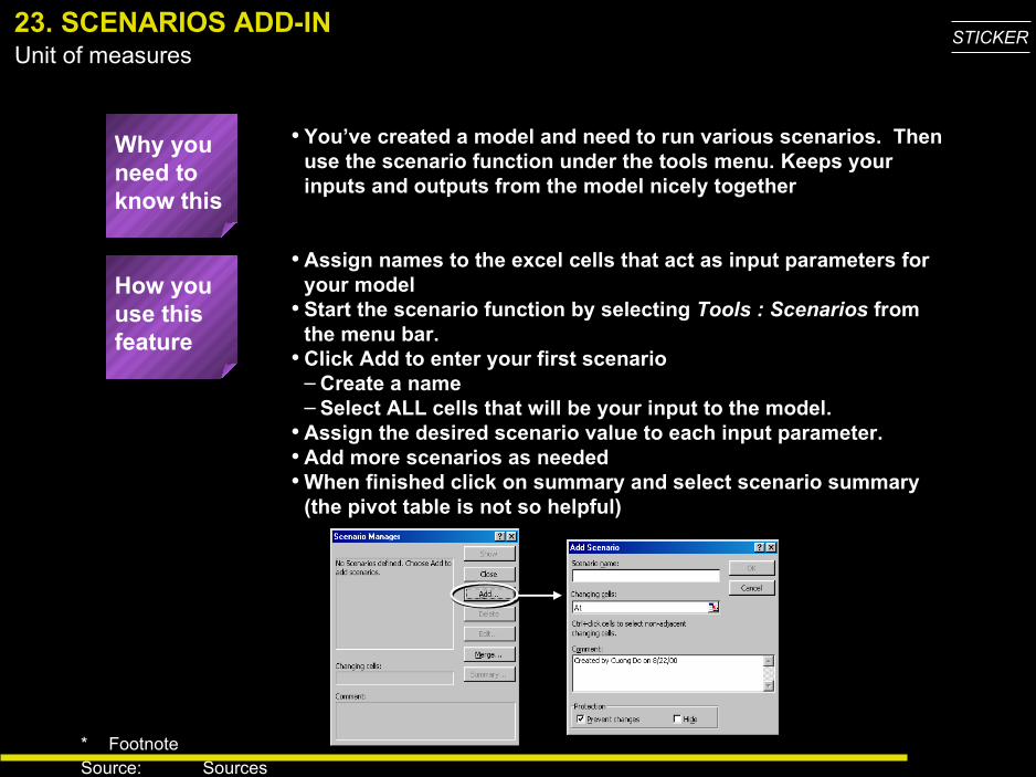
• You’ve created a model and need to run various scenarios. Then use the scenario function under the tools menu. Keeps your inputs and outputs from the model nicely together
• Assign names to the excel cells that act as input parameters for your model
• Start the scenario function by selecting Tools : Scenarios from the menu bar.
• Click Add to enter your first scenario– Create a name – Select ALL cells that will be your input to the model.
• Assign the desired scenario value to each input parameter.• Add more scenarios as needed• When finished click on summary and select scenario summary
(the pivot table is not so helpful)
23. SCENARIOS ADD-IN
How you use this feature
Why you need to know this
* FootnoteSource: Sources
Unit of measuresSTICKER
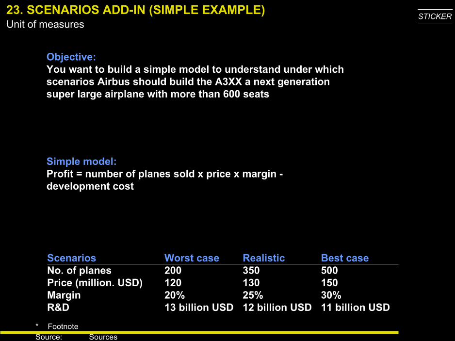
Objective:You want to build a simple model to understand under which scenarios Airbus should build the A3XX a next generation super large airplane with more than 600 seats
Simple model:Profit = number of planes sold x price x margin - development cost
Scenarios Worst case Realistic Best caseNo. of planes 200 350 500Price (million. USD) 120 130 150Margin 20% 25% 30%R&D 13 billion USD 12 billion USD 11 billion USD
23. SCENARIOS ADD-IN (SIMPLE EXAMPLE)
* FootnoteSource: Sources
Unit of measuresSTICKER
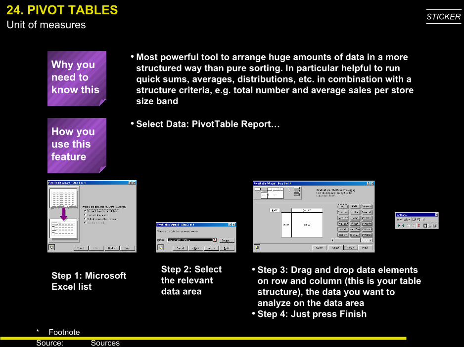
• Most powerful tool to arrange huge amounts of data in a more structured way than pure sorting. In particular helpful to run quick sums, averages, distributions, etc. in combination with a structure criteria, e.g. total number and average sales per store size band
• Select Data: PivotTable Report…
Step 1: Microsoft Excel list
Step 2: Select the relevant data area
• Step 3: Drag and drop data elements on row and column (this is your table structure), the data you want to analyze on the data area
• Step 4: Just press Finish
24. PIVOT TABLES
How you use this feature
Why you need to know this
* FootnoteSource: Sources
Unit of measuresSTICKER
•Draw a distribution chart for the number of stores per size in branches bucketed each 10 branch wide
•Arrange the store distribution by store size (each 10 branch) and daily tickets (each 100 tickets) and show the number of stores per each category
24. PIVOT TABLES (CONTINUED)
Exercise
* FootnoteSource: Sources
Unit of measuresSTICKER
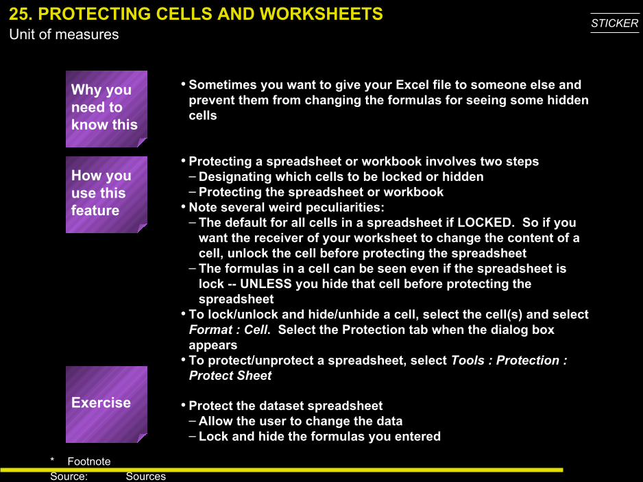
• Sometimes you want to give your Excel file to someone else and prevent them from changing the formulas for seeing some hidden cells
• Protecting a spreadsheet or workbook involves two steps– Designating which cells to be locked or hidden– Protecting the spreadsheet or workbook
• Note several weird peculiarities:– The default for all cells in a spreadsheet if LOCKED. So if you
want the receiver of your worksheet to change the content of a cell, unlock the cell before protecting the spreadsheet
– The formulas in a cell can be seen even if the spreadsheet is lock -- UNLESS you hide that cell before protecting the spreadsheet
• To lock/unlock and hide/unhide a cell, select the cell(s) and select Format : Cell. Select the Protection tab when the dialog box appears
• To protect/unprotect a spreadsheet, select Tools : Protection : Protect Sheet
• Protect the dataset spreadsheet – Allow the user to change the data– Lock and hide the formulas you entered
25. PROTECTING CELLS AND WORKSHEETS
How you use this feature
Exercise
Why you need to know this
* FootnoteSource: Sources
Unit of measuresSTICKER
•Avoid having to redo your work on multiple spreadsheets in a single workbook
•Select the first spreadsheet to be edited•Hold the Ctrl key while clicking on the additional
spreadsheets•Do your editing
•Try it
26. EDITING MULTIPLE WORKSHEETS SIMULTANEOUSLY
How you use this feature
Exercise
Why you need to know this
* FootnoteSource: Sources
Unit of measuresSTICKER
•Sometimes you would to color the output of cells in different colors, e.g. negative numbers in red, positive numbers in black, or add a frame, etc.
•Mark the relevant fields and select Format: Conditional Formatting
•Select the criteria for the format and adjust the format. You can actually change the font, the border and the color
•Click on Add to select additional criteria for the formatting
•Format a cell to be in red font, with blue background for negative numbers and in bold font with thick border, if the value is above 10
27. CONDITIONAL FORMATTING
Exercise
How you use this feature
Why you need to know this

* FootnoteSource: Sources
Unit of measuresSTICKER
•You have a huge pile of data and quickly want to find some specific information, e.g. all sets that meet a criteria or the top 10 items etc.
•Click into your table or better mark the data area and select Data: Filter: Autofilter
•Using the drop-down boxes per item allows you to display only specific filtered information
•Selecting multiple matches (up to 3 maximum with autofilter) you can narrow down your search
•Or add your own criteria for filtering by clicking on the custom criteria
•Find the stores who belong to the top 10% in terms of average sales per ticket AND the top 10 in terms of store size in branch
28. AUTOFILTER COMMAND
Exercise
How you use this feature
Why you need to know this
* FootnoteSource: Sources
Unit of measuresSTICKER
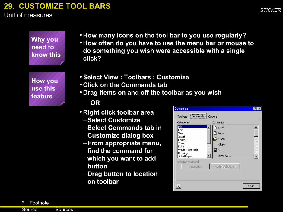
•How many icons on the tool bar to you use regularly?•How often do you have to use the menu bar or mouse to
do something you wish were accessible with a single click?
•Select View : Toolbars : Customize•Click on the Commands tab•Drag items on and off the toolbar as you wish
29. CUSTOMIZE TOOL BARS
How you use this feature
Why you need to know this
•Right click toolbar area–Select Customize–Select Commands tab in
Customize dialog box–From appropriate menu,
find the command for which you want to add button
–Drag button to location on toolbar
OR
* FootnoteSource: Sources
Unit of measuresSTICKER
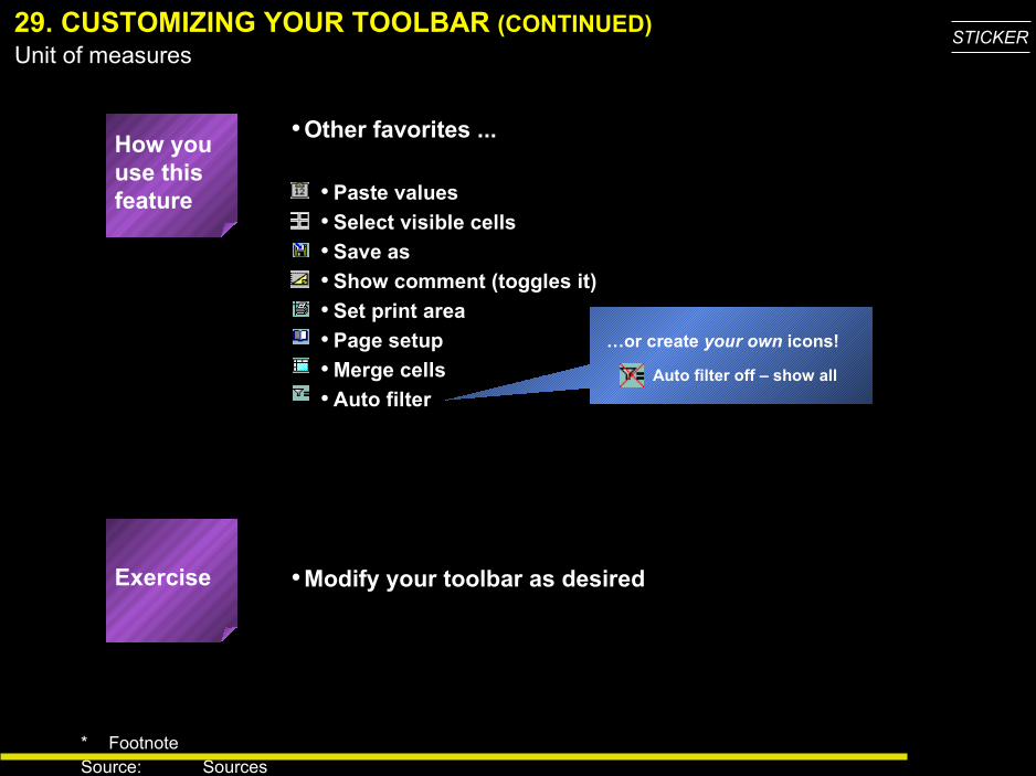
…or create your own icons!
Auto filter off – show all
29. CUSTOMIZING YOUR TOOLBAR (CONTINUED)
Exercise
How you use this feature • Paste values
• Select visible cells
• Save as
• Show comment (toggles it)
• Set print area
• Page setup
• Merge cells
• Auto filter
•Other favorites ...
•Modify your toolbar as desired
* FootnoteSource: Sources
Unit of measuresSTICKER
•How often do you use the menu bar to change the normal font or number formats?
•You can create the basic number and font formats you use regularly, save it as a template, and have Excel use that template every time you create a new workbook
•Create a workbook with the formatting you use regularly and save it under the name “Book” and Template format
•Move the “Book” template to the Microsoft Office : Office : Xlstart folder
•Create your default workbook
How you use this feature
Exercise
30. CHANGING DEFAULT WORKBOOK
Why you need to know this
* FootnoteSource: Sources
Unit of measuresSTICKER
•How often would you like to hide or unhide parts of a complex spreadsheet?
• If your answer is “very often”. You will like to group/ungroup function instead of the hide/unhide command, since you will be able to toggle between hidden or displayed columns or rows.
•Mark the row or column that you would like to “fold”, i.e. hide for the moment.
•Click on Data: Group and Outline: Group•To “fold” click now on the “minus” sign outside of your
column or row•You may also group or ungroup hierarchically
•Group some parts in your spreadsheet•Also try to remove the grouping
•Use the two “arrow” buttons, which you find on the pivot table toolbar (right click on any toolbar and select PivotTable)
31. GROUP/UNGROUP PARTS OF SPREADSHEETS
Exercise
Tip
How you use this feature
Why you need to know this
* FootnoteSource: Sources
Unit of measuresSTICKER
•Also find the Microsoft Actors more disturbing than helpful?
•Always popping up at the wrong moment
•Excel 97–Start the Windows Explorer–Go to the directory Program Files: Microsoft Office:
Office: Actors–Rename the directory “Actors” to “Dead Actors”
•Excel 2000–Go to Tools : Options : Edit and switch off „Provide
feedback with animation“
•Try to eliminate the Actors
32. SWITCH OFF THE MICROSOFT ACTORS
Exercise
How you use this feature
Why you need to know this
* FootnoteSource: Sources
Unit of measuresSTICKER
33. CLEAN UP TEXT
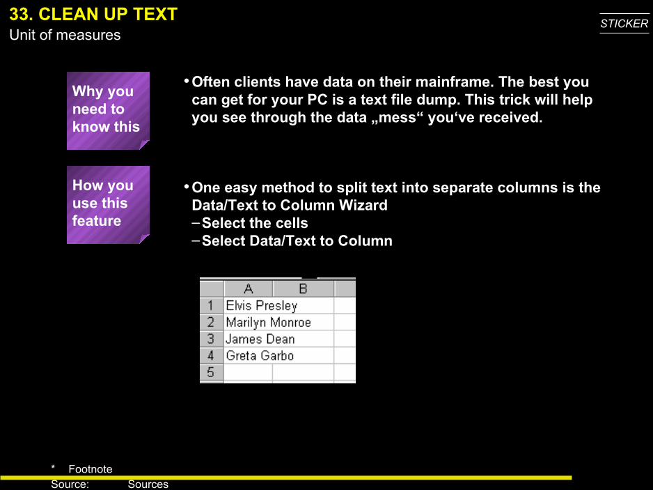
•One easy method to split text into separate columns is the Data/Text to Column Wizard–Select the cells–Select Data/Text to Column
How you use this feature
Why you need to know this
•Often clients have data on their mainframe. The best you can get for your PC is a text file dump. This trick will help you see through the data „mess“ you‘ve received.
* FootnoteSource: Sources
Unit of measuresSTICKER
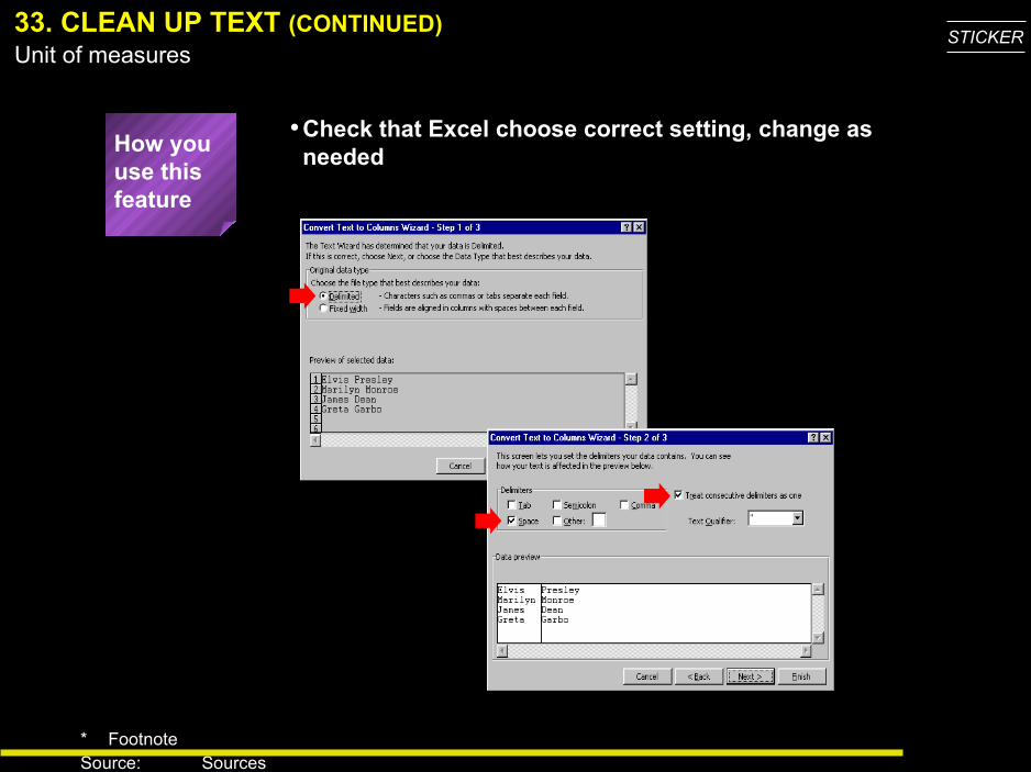
33. CLEAN UP TEXT (CONTINUED)
How you use this feature
•Check that Excel choose correct setting, change as needed
* FootnoteSource: Sources
Unit of measuresSTICKER
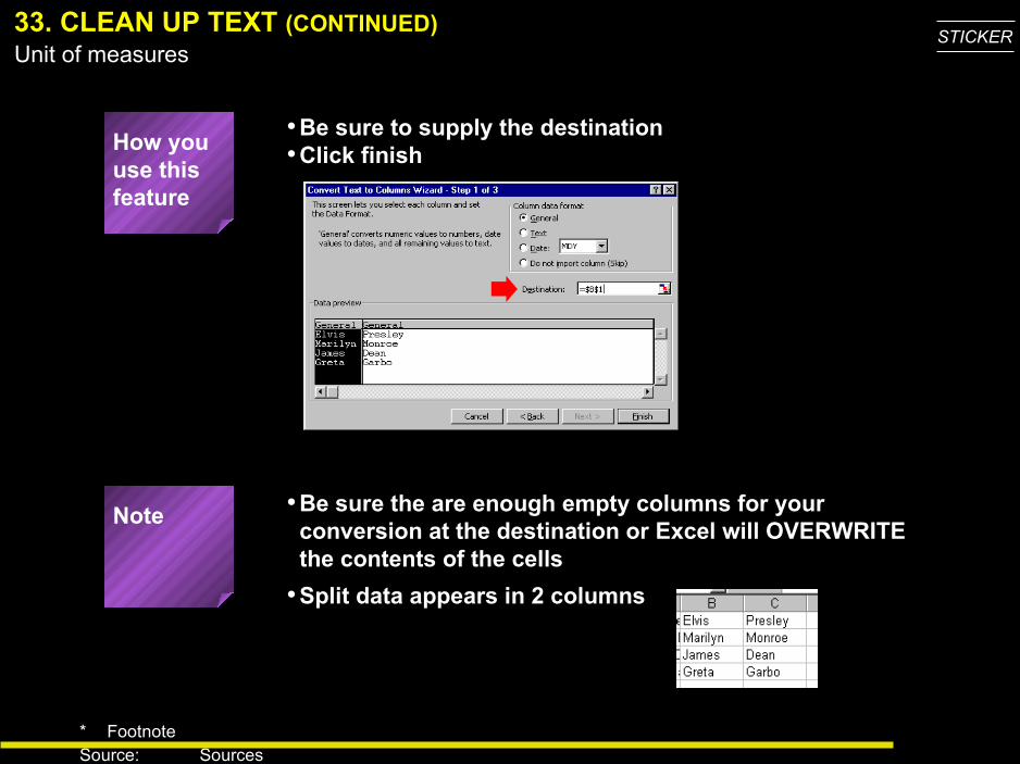
•Be sure the are enough empty columns for your conversion at the destination or Excel will OVERWRITE the contents of the cells
33. CLEAN UP TEXT (CONTINUED)
How you use this feature
•Be sure to supply the destination•Click finish
Note
•Split data appears in 2 columns
* FootnoteSource: Sources
Unit of measuresSTICKER
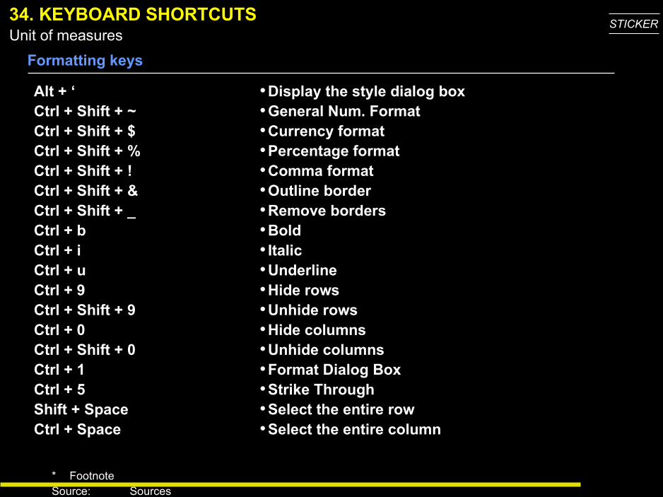
34. KEYBOARD SHORTCUTS
Alt + ‘Ctrl + Shift + ~Ctrl + Shift + $Ctrl + Shift + %Ctrl + Shift + !Ctrl + Shift + &Ctrl + Shift + _Ctrl + bCtrl + iCtrl + uCtrl + 9Ctrl + Shift + 9Ctrl + 0Ctrl + Shift + 0Ctrl + 1Ctrl + 5Shift + SpaceCtrl + Space
•Display the style dialog box•General Num. Format•Currency format•Percentage format•Comma format•Outline border•Remove borders•Bold• Italic•Underline•Hide rows•Unhide rows•Hide columns•Unhide columns•Format Dialog Box•Strike Through•Select the entire row•Select the entire column
Formatting keys
* FootnoteSource: Sources
Unit of measuresSTICKER
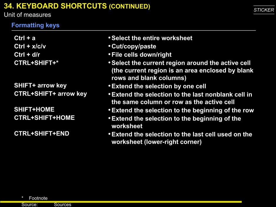
34. KEYBOARD SHORTCUTS (CONTINUED)
Ctrl + aCtrl + x/c/vCtrl + d/rCTRL+SHIFT+*
SHIFT+ arrow keyCTRL+SHIFT+ arrow key
SHIFT+HOMECTRL+SHIFT+HOME
CTRL+SHIFT+END
•Select the entire worksheet•Cut/copy/paste•File cells down/right•Select the current region around the active cell
(the current region is an area enclosed by blank rows and blank columns)
•Extend the selection by one cell•Extend the selection to the last nonblank cell in
the same column or row as the active cell•Extend the selection to the beginning of the row•Extend the selection to the beginning of the
worksheet•Extend the selection to the last cell used on the
worksheet (lower-right corner)
Formatting keys
* FootnoteSource: Sources
Unit of measuresSTICKER
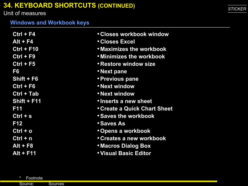
Ctrl + F4Alt + F4Ctrl + F10Ctrl + F9Ctrl + F5F6Shift + F6Ctrl + F6Ctrl + TabShift + F11F11Ctrl + sF12Ctrl + oCtrl + nAlt + F8Alt + F11
•Closes workbook window•Closes Excel•Maximizes the workbook•Minimizes the workbook•Restore window size•Next pane•Previous pane•Next window•Next window• Inserts a new sheet•Create a Quick Chart Sheet•Saves the workbook•Saves As•Opens a workbook•Creates a new workbook•Macros Dialog Box•Visual Basic Editor
Windows and Workbook keys
34. KEYBOARD SHORTCUTS (CONTINUED)
* FootnoteSource: Sources
Unit of measuresSTICKER
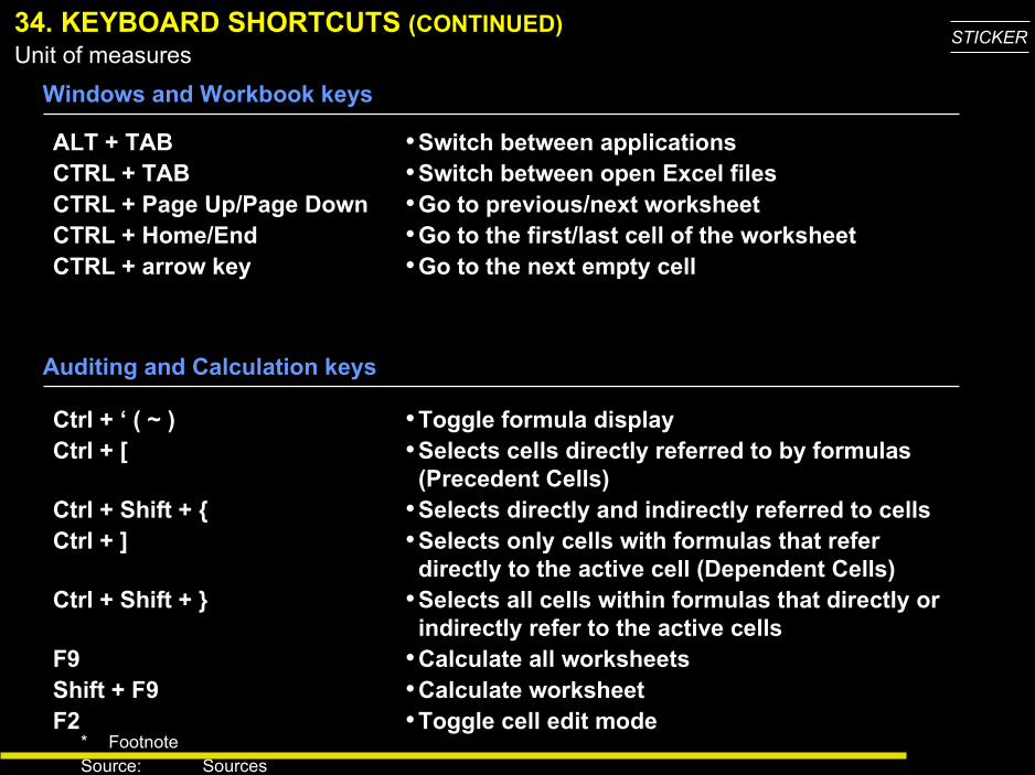
34. KEYBOARD SHORTCUTS (CONTINUED)
ALT + TABCTRL + TABCTRL + Page Up/Page DownCTRL + Home/EndCTRL + arrow key
•Switch between applications•Switch between open Excel files•Go to previous/next worksheet•Go to the first/last cell of the worksheet•Go to the next empty cell
Windows and Workbook keys
Auditing and Calculation keys
Ctrl + ‘ ( ~ )Ctrl + [
Ctrl + Shift + {Ctrl + ]
Ctrl + Shift + }
F9Shift + F9F2
•Toggle formula display•Selects cells directly referred to by formulas
(Precedent Cells)•Selects directly and indirectly referred to cells•Selects only cells with formulas that refer
directly to the active cell (Dependent Cells)•Selects all cells within formulas that directly or
indirectly refer to the active cells•Calculate all worksheets•Calculate worksheet•Toggle cell edit mode
* FootnoteSource: Sources
Unit of measuresSTICKER
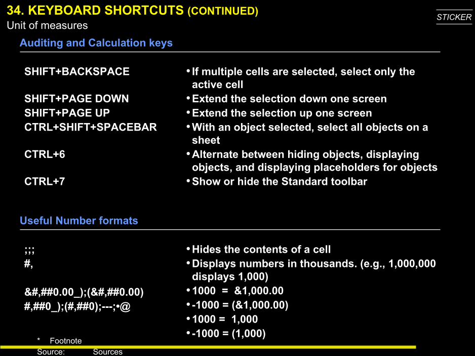
34. KEYBOARD SHORTCUTS (CONTINUED)
Auditing and Calculation keys
SHIFT+BACKSPACE
SHIFT+PAGE DOWNSHIFT+PAGE UPCTRL+SHIFT+SPACEBAR
CTRL+6
CTRL+7
• If multiple cells are selected, select only the active cell
•Extend the selection down one screen•Extend the selection up one screen•With an object selected, select all objects on a
sheet•Alternate between hiding objects, displaying
objects, and displaying placeholders for objects•Show or hide the Standard toolbar
Useful Number formats
;;;#,
&#,##0.00_);(&#,##0.00)#,##0_);(#,##0);---;•@
•Hides the contents of a cell•Displays numbers in thousands. (e.g., 1,000,000
displays 1,000)•1000 = &1,000.00• -1000 = (&1,000.00)•1000 = 1,000• -1000 = (1,000)
* FootnoteSource: Sources
Unit of measuresSTICKER
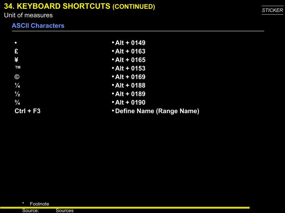
34. KEYBOARD SHORTCUTS (CONTINUED)
ASCII Characters
•£¥™©¼½¾Ctrl + F3
•Alt + 0149•Alt + 0163•Alt + 0165•Alt + 0153•Alt + 0169•Alt + 0188•Alt + 0189•Alt + 0190•Define Name (Range Name)
* FootnoteSource: Sources
Unit of measuresSTICKER
35. FINAL THOUGHTS
• Structure, structure, structure. Should know this anyway, since you‘re ED keeps telling you this every day
• Keep Inputs, Processing and Outputs on different worksheets of your Excel file (IPO principle)
• Name universal variables, e.g., WACC instead of $AH264
• Use color-coding, but don‘t overdo it. Excel is not a crayon-box.
• Save cautiously, but frequently. Keep different versions and backup (network, floppy disk). We‘ve seen too many models disappearing the night before the progress review. The 35 Excel tricks won‘t help then any more.