What Drives the Performance of Convertible-Bond Funds?

1

What Drives the Performance of Convertible-Bond Funds?

Manuel Ammann, Axel Kind, and Ralf Seiz∗

March 2007

Abstract

This paper examines the performance of US mutual funds investing primarily in convertible bonds. Although convertible-bond funds are popular investment vehicles, their return process is not well understood. We contribute an analysis of the complete universe of US convertible-bond funds proposing a set of multi-factor models for the return generating process. In spite of the well-known hybrid nature of convertible bonds, the return process of convertible-bond funds cannot be fully explained by factors typically related to stock and bond markets. Thus, we consider additional variables accounting for the option-like character of convertible bonds. Surprisingly, multivariate cross-sectional analyses show the existence of a significant positive relationship between fund's performance and its asset composition. We show that this result can be explained by factors related to investment opportunities in the convertible-bond market and trading strategies related to convertible arbitrage, as typically performed by hedge funds. Overall, convertible-bond funds have a performance as measured by alpha that is comparable to passive investment strategies in stocks, bonds, and convertible-bonds. This average performance is the result of weak selection skills and successful timing in trading strategies closely related to convertible arbitrage.

Keywords: Mutual Funds, Performance, Hybrid Securities, Convertible Bonds. JEL classification: G12, G13, G15.

∗ Manuel Ammann, Axel Kind, and Ralf Seiz are at the Swiss Institute of Banking and Finance, University of St. Gallen, Rosenbergstrasse 52, 9000 St.Gallen, Switzerland. Tel: +4171-224-7090, Fax +4171-224-7088, Email: [email protected], [email protected], [email protected]. Financial support by the Swiss National Science Foundation (SNF) and the Research Fund (GFF) is gratefully acknowledged. We thank Yakov Amihud, Edwin Elton, Stephen Figlewski, Georg Hübner, Christian Koziol, Lorne Switzer, Michael Steiner, and participants at the 2006 Northern Finance Association Meeting in Montreal, the 2006 German Finance Association Meeting in Oestrich-Winkel, and the 2006 Topics in Finance Seminar in St. Moritz for their very helpful comments.

2

1 Introduction

With an estimated global market volume of more than 40 billion US dollars in 2005,1

convertible-bond funds (CBFs) are an important constituent of the investment universe.

Convertible bonds are often seen by professionals in the asset management industry as a

distinct asset class2. Interestingly, while both academics and practitioners have extensively

studied the performance and return characteristics of individual stocks, bonds, equity

funds, and bond funds,3 little attention has been dedicated to studying and explaining the

performance of funds investing in convertible bonds. From a theoretical perspective, as

convertible-bond funds invest in derivative instruments, a model explaining returns has to

account for non-linear payoffs and dynamic strategies. In this context, it is a relevant

question whether in addition to stock and bond factors, there exist factors specific to

convertible-bond funds. This issue has also important practical implications for risk

management, portfolio optimization, and performance measurement.

This paper contributes the first empirical study of the US CBF market. It investigates the

complete universe of convertible-bond funds in the US consisting of 114 CBFs in the

period of 1985-2004. The employed data set is free of survivorship bias. We provide a

detailed description of US convertible-bond funds and propose a set of models suitable for

explaining their returns. In particular, we discuss and empirically test several methods to

account for the option-like payoff structure of convertible bonds. Under a large set of

plausible data generating models, we find a significant and positive relation between the

fund's performance and its asset composition. We explain this surprising result by relating

CBF returns to the investment opportunity set available in the convertible bond market and

to arbitrage strategies as typically performed by hedge funds.

1 Estimation is based on data provided by Lipper Global Fund Screener, CRSP, and Datastream.

2 The reader may refer to Lummer and Riepe (1993), for one of the first studies taking the view that convertible bonds represent an own asset class.

3 For the return characteristics of common stocks, see Chen, Roll and Ross (1986), Fama and French (1992, 1993), Carhart (1997), Burmeister and Wall (1986), Elton, Gruber and Blake (1999), Ferson and Schadt (1996), among others. For bonds, see Elton, Gruber and Blake (1999). For both asset classes, see Fama and French (1993).

3

A convertible bond gives the holder the right to exchange (convert) a bond for a certain

number of shares of the bond-issuing company. Simplistically, it can be viewed as a

combination of a straight bond and a call option on the equity of the issuing firm. Thus,

besides combining attributes of fixed-income securities and equities, convertible bonds

present their own return characteristics related to the option-like nature of the instruments.

We examine performance models for convertible-bond funds that include factors typically

related to stocks and bonds as well as factors capturing the option-like character of

convertible bonds. Further, we evaluate the performance of convertible-bond funds in

dependence on selected fund characteristics. We use the same multivariate cross-sectional

methodology as in Kacperczyk, Sialm, and Zheng (2005) and verify the robustness of our

results by applying multivariate cross-sectional analyses for sub-periods and alternative

risk adjustments. The proposed models are able to capture a large part of the return process

of convertible-bond funds. However, the analysis indicates that the common factors for

stocks, bonds, and convertible bonds are not sufficient to explain the cross-sectional

variation in convertible bond fund returns. More precisely, cross-sectional abnormal

returns are found to be significantly positively (negatively) related to the fund's convertible

bond (equity) holdings. Most interestingly, after introducing either a factor capturing the

investment opportunity set in the convertible bond market or a convertible bond arbitrage

index, cross-sectional abnormal returns cease to depend on funds' asset holdings. This

result confirms the close relation between CBFs, convertible bonds, and convertible

arbitrage.

When compared to passive investment strategies, CBFs deliver an average performance.

CBFs seem to implement dynamic trading strategies related to convertible arbitrage but,

overall, they are less successful than convertible-arbitrage hedge funds. Moreover, CBFs

seem to increase their convertible-arbitrage related activities in phases when this strategy

performs well, i.e. when investment opportunities in the convertible-bond market are good.

This successful timing activity compensates the weak selection skills of CBFs' portfolio

managers in the stock, bond, and convertible-bond market.

4

The structure of the paper is as follows: Section 2 describes the CBF market and the data

set used in the article. Section 3 describes the factors that possibly drive the performance of

CBFs. Section 4 proposes and tests the factor models. Section 5 proposes and tests an

additional model set extended by convertible arbitrage related aspects. Section 6 discusses

the performance of CBF. Section 7 concludes.

5

2 U.S. Convertible-bond funds

In this paper, we investigate the U.S. market for convertible-bond funds (CBFs) between

October 1985 and December 2004. According to the CRSP (Center for Research in

Security Prices)4 survivorship-free database, 129 CBFs are traded in this period, out of

which 14 are closed-end funds. In the same time, 41 CBFs were terminated, resulting in 73

active open-end CBFs with a market volume of 10.6 billion US dollars as of December

2004. As depicted in Table I, the final sample of CBFs analyzed in this study includes 114

open-end convertible-bond funds.

Interestingly, CBFs do not exclusively invest in convertible securities, such as convertible

bonds (38% average holding) and preferred stocks (20%), but also in stocks (11%) and

bonds (13%). Further, a portion of the funds are so called long-short CBFs, which are

allowed to have short positions in stocks but are nevertheless part of the mutual fund

universe defined by the 1940 Investment Advisory Act. Convertible-bond funds have on

average total net assets of $120 million, new money growth of 2% per month, and expense

ratios of 1.5%, which lies in between the expense ratios commonly raised by bond funds

and stock funds (cf. Table II).

4 The CRSP database includes information on fund objectives, fund returns, total net asset values, expense ratios, age of the funds, status of the fund (dead or active), asset compositions (e.g. percentages invested in convertible bonds, stocks and bonds), and other fund characteristics. Returns and total net assets are reported monthly, fund characteristics such as asset compositions and expense ratios are generally reported on a yearly basis.

6

Table I

US Convertible Bond Fund Selection and Yearly Statistics

Total number of US convertible bond funds in CRSP database 129

Closed US convertible bond funds in CRSP database 14

US convertible bond funds with no Return Data in CRSP database 1

Number of selected active funds (current status) 73

Number of selected dead funds (current status) 41

Total number of funds in this study 114

YearNumber of active

convertible bond funds (end of year)

TNA (end of year)(in $millions)

1985 7 8041986 12 16001987 16 33341988 23 28471989 23 25031990 22 16621991 19 17251992 23 26661993 25 36731994 28 33641995 35 38201996 38 44771997 46 57291998 45 56441999 47 63122000 52 67682001 60 59402002 60 52462003 63 93192004 73 10628

Panel B: Summary of active funds: 1985-2004

Panel A: Selection of funds of the CRSP Survivor-Bias Free US Mutual Fund Database: 1985-2004

The data set has been created by the CRSP Survivorship Bias Free US Mutual Fund Database. Panel A describes the fund selection process. The original CRSP sample in the period between 1985 and 2004 contained 129 US convertible-bond funds. We eliminated 14 closed funds and a fund with no return data. With these exclusions, our final sample includes 114 convertible-bond funds (73 active convertible-bond funds and 41 dead funds). Our final sample spans the period between October 1985 and December 2004. Panel B gives an overview of the number of active funds and total net assets in each year of the sample in the period between October 1985 and December 2004.

7

Table II

Convertible Bond Fund Summary Statistics

MeanStdev of

mean Min Max

Avg TNA ($ millions) 120.0 255.4 0.001 2507Avg New Money Growth (NMG) (in % per month) 2% 21% -513% 550%Avg Expense Ratio (EXP) (% per year) 1.5% 0.6% 0.01% 3.8%Avg Age (in years) 7.3 7.3 0.1 48.9

Avg % in Stocks (S) 11% 17% -68% 124%Avg % in Bonds (incl. Convertibles) (B) 51% 25% 0% 123%Avg % in Convertible Bonds (CB) 38% 28% 0% 98%Avg % in Convertibles - % in Stocks (CB-S) 27% 34% -96% 129%Avg % in Bonds (incl. Convertibles) - % in Stocks (B-S) 47% 27% -96% 191%Avg % in Preferred Stocks 20% 10% 0% 82%Avg % in Cash 6% 10% -2% 100%

Panel A: Main Convertible Bond Fund Characteristics

Panel B: Main Asset Composition of Convertible Bond Funds

This table reports summary statistics of the convertible-bond funds of the CRSP (Center for Research in Security Prices) Survivor-Bias Free US Mutual Fund Database investigated in this study. The table shows attributes of 114 US convertible-bond funds from 1985-2004. The mean is the cross-sectional average of time-series averages attributes. The stdev of mean is the cross-sectional standard deviation of the mean. Min and Max are the time-series and cross-sectional minimum and maximum. Panel A shows the main convertible bond fund characteristics and Panel B shows the asset composition of the funds. TNA is total net asset value; NMG (New Money Growth) is the percentage change in TNA adjusted for investment return. EXP is the expenses ratio. TNA are reported monthly, whereas the asset compositions are generally reported yearly (or even more often).

8

Before addressing the performance of CBFs by asset pricing models, it is worth giving a

first look at some simple, model-free performance measures of CBFs and possible

benchmarks. Table III presents a comparison of realized returns, volatilities, Sharpe ratios,

and Sortino ratios for broad stock, bond, convertible-bond, and convertible-arbitrage

indices. Several observations can be made. First, for all periods considered, returns and

volatilities of CBFs are between the corresponding values for stocks and bonds. This is not

surprising, given the hybrid nature of convertible bonds. Second, the Sharpe ratios of an

equally-weighted portfolio of CBFs are always below the stock and straight-bond

counterparts, which is indicative of a poor risk-return ratio. Third, the Sortino ratios, which

only consider negative returns (below 0%) when measuring risk, seem to confirm the poor

performance of CBFs. This stands in contrast to the common view that convertible bonds

offer a downside protection through the so-called bond floor, the bond-value component of

the convertible. However, a Jarque-Bera test statistics supports the results above, because

59% of the convertible-bond funds in our sample show normally distributed returns.

9

Table III Convertible Bond Fund Performance

CB Funds Stocks Bonds Convertible Bonds

Convertible Arbitrage HF

Return (p.a.) 9.4% 13.1% 8.2%Volatility (p.a.) 10.8% 15.7% 4.8%Downside-Volatility (p.a.) 12.7% 17.9% 4.6%Sharpe Ratio 0.44 0.54 0.73Sortino Ratio 0.38 0.47 0.77

Return (p.a.) 9.5% 12.6% 7.8% 10.6%Volatility (p.a.) 10.2% 14.5% 4.6% 11.3%Downside-Volatility (p.a.) 11.0% 15.6% 4.5% 12.3%Sharpe Ratio 0.49 0.56 0.73 0.55Sortino Ratio 0.46 0.52 0.75 0.50

Return (p.a.) 8.6% 11.5% 6.5% 9.0% 9.4%Volatility (p.a.) 11.3% 15.7% 4.6% 12.5% 4.7%Downside-Volatility (p.a.) 12.1% 17.6% 4.8% 13.3% 6.3%Sharpe Ratio 0.42 0.49 0.59 0.42 1.19Sortino Ratio 0.40 0.43 0.56 0.39 0.88The threshold for the Downside-Volatility and the Sortino ratio is set to 0%.

Panel A: 10/1985 - 12/2004

Panel B: 1/1988 - 12/2004

Panel C: 1/1994 - 12/2004

This table reports summary statistics of the convertible-bond funds of the CRSP (Center for Research in Security Prices) Survivor-Bias Free US Mutual Fund Database investigated in this study (CB Funds). The table shows the performance of 114 US convertible-bond funds from 1985-2004. (CB Funds) are the equally weighted returns in the CRSP convertible bond fund sample. (Stocks) is the value-weighted return on all NYSE, AMEX, and NASDAQ stocks (from CRSP). (Bonds) is the return on the Lehman US aggregated Government/Credit Bond Index. (Convertible Bonds) is the return on the Merrill Lynch All US Convertible Bond Index. (Convertible Arbitrage HF) is the return on the CSFB/Tremont Convertible Arbitrage Hedge Fund Index. The Sharpe ratio is calculated by using a one-month Treasury bill rate (from Ibbotson Associates) and the threshold for calculating the Sortino ratio (Downside Volatility) is set to 0%.

10

3 What Factors Drive the Performance of Convertible-bond funds?

In this section, we examine factors that are possibly qualified to explain CBF returns.

Overall, we classify risk factors into four categories: (i) stock factors, (ii) bond factors, (iii)

option factors, and (iv) fund factors.

3.1 Stock Factors

CBFs are likely to be influenced by stock factors because they invest directly in equities

and because the price of convertible securities is intrinsically related to the underlying

stock. In line with the standard four-factor model proposed by Carhart (1997), we consider

the following risk factors: (i) MARKET, is the value-weighted return on all NYSE, AMEX,

and NASDAQ stocks minus the one-month Treasury bill rate; (ii) SMB is the return

difference between small and large-capitalization stocks; (iii) HML is the difference

between high and low book-to-market stocks; and (iv) UMD is the return difference

between stocks with high and low past returns.

3.2 Bond Factors

Similarly, CBFs are likely to be influenced by bond factors because they invest directly in

straight bonds and cash instruments and because convertible securities have a bond

component. Following Fama and French (1993), Burmeister and Wall (1986), and Blake,

Elton and Gruber (1999), we consider the following four bond risk factors: (i) TERM is a

proxy for the unexpected changes in interest rates and is defined as the return of the

Lehman US Government Long Bond Index minus the one-month Treasury bill rate; (ii)

DEFT is a proxy for the default factor and is defined as the return on the Lehman US

Corporate Long Bond Index minus the return of the Lehman US Government Long Bond

Index5; (iii) HY captures both a term and a credit premium and is defined as the return on

the Merrill Lynch US High Yield Index.6; Finally, (iv) BOND is the excess return of a

broad bond index (Lehman US aggregated Government/Credit Bond Index).

5 The definitions of the term structure factor (TERM) and the default factor (DEFT) are similar to the study of Fama and French (1993).

6 The use of a high yield index (HY) is similar to the study of Elton, Gruber and Blake (1999)

11

3.3 Option Factors

The option embedded in convertible bonds to exchange them into shares of the underlying

stock resembles a call option. For this reason, it seems plausible that CBF returns may

display a dependence on factors affecting option prices. According to standard option

pricing theory, the value of non-linear derivatives depends on the volatility of the

underlying. Further, a multitude of articles in the field of financial econometrics documents

the fact that volatility of single securities and the aggregate market changes over time. For

those two reasons, we expect implied volatility on the aggregate market to capture the

variation of CBF returns. Motivated by the methods of Henriksson and Merton (1981) and

Treynor and Mazuy (1966), we examine non-linear payoff factors and test whether they are

significant. Additionally, similar to Agarwal and Naik (2004), we extend the analysis of

non-linear factors for convertible bond fund returns to option-based factors consisting of

liquid at-the-money (ATM) and out-of-the-money (OTM) European call and put options

on the S&P 500 index trading on the Chicago Mercantile Exchange. The process of

generating the call and put time series works as follows: On the first trading day in

January, buy an ATM (OTM) call or put option on the S&P 500 index that expires in

February.7 On the first trading day in February, sell the option bought a month ago and buy

another ATM (OTM) call or put option on the S&P 500 index that expires in March.

Repeating this trading pattern every month provides the time series of returns. We select

the ATM option as the one whose present value of the strike price is closest to the current

index value. We select the OTM put option to be the one with the next lower strike price.

Using price data from OptionMetrics, we compute monthly returns to these option-based

risk factors for the period of January 1996 to December 2004. By using a convertible-bond

index, we intend to capture all residual pricing-relevant influences on convertible bonds

funds.

Summing up, we analyze six possible factors: (i) VOLA is the return on the CBOE

Volatility VXO Index; (ii) NL1 is the maximum of zero and the value-weighted return on

all NYSE, AMEX, and NASDAQ stocks minus the return on the Lehman US aggregated

7 The time to maturity of the options is between one and two months when the options are bought. The results remain similar when the time to maturity is between two and three months when the options are bought.

12

Government/Credit Bond Index, max(0,MARKET-BOND); (iii) NL2 is the squared value-

weighted return on all NYSE, AMEX, and NASDAQ stocks minus the one-month

Treasury bill rate, (MARKET)2; (iv) ATM is the return on a dynamic portfolio of at-the-

money call and put options; (v) OTM is the return on a dynamic portfolio of out-of-the-

money call and put options; and (vi) CBI is the return on the Merrill Lynch All US

Convertible Bond Index.

3.4 Fund Factors

The last category of risk factors arises from specific trading strategies carried out by CBF

fund managers. In particular, we are interested in capturing variations of convertible-bond-

fund returns arising from convertible arbitrage or related convertible-picking strategies (the

long part of a typical long short convertible arbitrage strategy). For this purpose, we choose

the returns on the CSFB/Tremont Convertible Arbitrage Index, CBAI. Additionally,

Agarwal et al. (2006) argue that convertible-arbitrage hedge funds play an important role

in supplying liquidity to the convertible-bond market. They argue that convertible-

arbitrage hedge funds behave like liquidity providers to the convertible-bond market and

demonstrate the importance of supply-demand effects in determining the returns of hedge

fund strategies. Thus, similar to Agarwal et al. (2006), we estimate the net supply of

convertible bonds by aggregating every month the market capitalization of convertible

bonds traded in the US and subtracting the assets under management in US convertible-

bond funds8. We approximate the demand for convertible bonds by aggregating the total

AuM of all convertible arbitrage hedge funds in the TASS database at the end of each

month. The ratio of net supply and demand, SD, can be considered as the investment

opportunities available in the convertible bond market. Agarwal et al. (2006) show that

after accounting for the investment opportunities, convertible arbitrage hedge funds no

longer deliver abnormal returns. They further show that the risk-adjusted returns of

convertible arbitrage hedge funds are affected by the investment opportunities (supply and

demand) in the convertible bond market.

8 We use the "UBS US Convertible Bond Index" as a proxy for the market capitalization of US convertible bonds and the AuM data for the convertible-bond funds is from the CRSP mutual fund database.

13

3.5 Time-Varying Factor Loadings

Usually, asset pricing models linearly relate excess returns to a set of risk factors in the

following way:

Ri,t - RF,t = αi + Σk βki⋅Fk

t +ei,t , (1)

where Ri,t - RF,t are excess returns of security i over the risk free rate from time t-1 to time

t, Fkt are the explanatory factors in the performance model, βk

i are the constant factor

loadings, αi are the measures of the abnormal performance, and ei,t are independent

normally distributed errors. While such model specifications are still widely used, a

number of authors have questioned the assumption of constant factor loadings, βki. For

instance, Ferson and Schadt (1996), Jagannathan and Wang (1996), Berk, Green, and Naik

(1999), Lettau and Ludwigson (2001), and more recently Santos and Veronesi (2004) and

Ang and Chen (2005) have proposed models with time-varying betas. These authors

suggest several economic reasons that might cause time variability, such as the business

cycle, changes in financial leverage, technology shocks, or, in the case of mutual fund

returns, the trading behavior of managers. Interestingly, convertible bonds have an even

more fundamental reason for displaying time-variability of betas. In fact, their sensitivity

towards market movements can range from zero, as in the case of a deep out-of-the money

convertible, to values even larger than one, for deep in-the-money convertibles issued by

high-beta firms.

A simple example shall illustrate the time-variability of convertible-bond betas, which we

refer to as the delta effect of convertibles. We consider stocks, straight bonds, and

convertible bonds in an economy with constant interest rates. Stock returns are assumed to

follow a data generating process in accordance to the CAPM:

Ri,t = RF,t + βi ⋅ (RM,t - RF,t) + ei,t, with ei ~ N(0, σi) i.i.d.

14

The return of the aggregate stock market is equal to a constant market price of risk (MPR)

plus a normally distributed shock:

RM,t = MRP + eM,t, with eM ~ N(0, σM) i.i.d.

If we assume that the convertible bond is not exchangeable into the stock prior to maturity,

it can be considered as a combination of a straight bond plus a call option.9 Thus the

market sensitivity of the convertible bond towards the market, βconv, can be expressed as:

equityconv conv equityconv conv equity

convM equity M

RR R PPR R R

β β∂∂ ∂

= = ⋅ = Δ ⋅ ⋅∂ ∂ ∂

(2)

where Rconv, RM and Requity are returns of the convertible bond, the market portfolio, and

the stock of the company; Pequity and Pcall are the prices of the equity and the convertible

bond, and Δcall is the delta of the convertible bond, which is, in this particular example,

equivalent to the delta of a standard call option. Since the delta of an option changes over

time, also the beta of a convertible bond, i.e. its sensitivity towards the market, will change

over time. Thus, employing a constant beta model, such as the one in Equation (2), for

estimating the “true” beta of a convertible bond, can generate inaccurate results.

The finance literature has proposed several approaches to deal with the issue of time-

varying betas: (i) rolling regressions (e.g. Sirri and Tufano, 1992), (ii) instrumental

variables (e.g. Ferson and Schadt, 1996), and (iii) latent variables (e.g. Ang and Chen,

2005). In this paper, we address the issue by employing rolling regressions and models

with latent variables, which we estimate using Kalman filtering:10

9 For the sake of simplicity, we assume that the issuing company has no credit risk, the convertible bond has no callability, no putability, and it is only exercisable at maturity (European-style convertibility). While such characteristic are usually not given in practice, relaxing them increases the complexity of the pricing task but does not qualitatively alter the results of this example.

10 The recent literature favours the use of latent variables (see Ang and Chen, 2005). Rolling regressions provide an approximation of time-varying betas which is rather ad hoc. On the other hand, as noted by Harvey (2001), the choice of instruments in modelling time-varying betas is to a large extent arbitrary and results may vary widely depending on the instruments used.

15

Ri,t -RF,t = αi,t + βi,t⋅ (RM,t - RF,t) + Σk βki⋅Fk

t + ei,t, with ei ~ N(0, σi), and

βi,t = β0 + φ βi,t-1+ ηi,t , with ηi,t ~ N(0, σβi),

where the first equation is the measurement equation and the second one is the state

equation of the latent factor loading (beta). While several factors could potentially display

time-varying loadings, we choose to restrict ourselves to one latent factor, arguably the

market factor, in order to work with reasonably parsimonious models.

Figure 1, Panel A shows the evolution over time of the convertible bond beta, βconv, (black

solid line) for one simulated path. The standard linear factor model cannot capture this

pattern but estimates instead a constant beta, which can be interpreted as an average of the

true time-varying beta. For the displayed path, the root-mean squared error of beta amounts

to 0.21. By employing rolling regressions, an important portion of the variation of βconv can

be captured (dotted line) and the RMSE of betas can be reduced to 0.17. However, the

initial window of data is lost and the estimated beta lags behind the true beta. Overall, the

best fit is obtained with the latent model (dashed line) with a RMSE of 0.09.

16

0 20 40 60 80 1000

0.2

0.4

0.6

0.8

1

1.2

Months

Load

ing

(bet

a)

correct betaconstant beta36−month rolling window betatime−varying beta (Kalman filter)

Figure 1

Actual and Estimated Loadings of Convertible-Bond Funds

Panel A: Straight Convertible-Bond Fund Panel B: Mixed Convertible-Bond Fund

0 20 40 60 80 1000

0.2

0.4

0.6

0.8

1

1.2

Months

Load

ing

(bet

a)

correct betaconstant beta36−month rolling window betatime−varying beta (Kalman filter)

This figure shows the development over a period of ten years (simulated with monthly frequency) of the market beta of a convertible bond fund (solid lines). Panel A refers to a fund that consists simply of one convertible bond. Panel B, refers to a fund that invests two convertible bonds (each with a 25% weight), the two underlying stocks (each with a weight of 12.5%), and a riskles zero-beta bond (25%). All convertible bonds are non-callable and non-putable. They have a maturity of ten years and can be converted by the investor solely at maturity (European-style convertibles). The theoretical beta is displayed as solid black line. According to Equation (2), the theoretical beta corresponds of three multiplicative components: the equity beta, the delta of a call option with a strike price equal to the notional of the convertible bond and written on the stock of the issuing firm, and the ratio of stock price to convertible bond price. Further, three commonly used estimation models are applied to estimate beta by solely using observed fund returns and market returns: (i) a simple OLS regression with constant beta (dashed horizontal line), (ii) a rolling OLS regression with a 36-month window (dotted line), and (iii) a model with a time-varying latent betas estimated by Kalman filtering (dashed line). The following assumptions underlie this example. The returns of the underlying stocks linearly depends on the market return (CAPM assumption). The underlying stocks have an annualized idiosyncratic volatility of 10% and betas of 1.5 (Panel A), 1.1, and 0.9 (Panel B). Market returns are independent and normally distributed with an annual drift of 8% and standard deviation of 15%. The random draws for the market and one stock are held constant in both graphs.

17

In spite of the arguments in favor of explicitly modeling time-varying betas, this issue

might be far less relevant for the purposes of this study. First, the example in Figure 1,

Panel A, is rather extreme because the chosen stock beta of 1.5 is comparatively high and

the maturity of the convertible bond reaches zero, favoring extreme values of delta.

Second, CBFs typically hold several convertible securities in their portfolios, reducing

variability in the overall funds' market beta through diversification. Third, CBFs are likely

to adjust periodically their portfolios in order to substitute redeemed maturing issues and

hold certain portfolio characteristics, such as duration and moneyness, constant over time.

Finally, as documented in Section 2, CBFs also heavily invest in straight bonds and regular

stocks, instruments that display a much less pronounced variation in market beta. To get a

first insight about the effects of considering CBFs with more realistic portfolios, Figure 1,

Panel B displays the evolution of beta for CBF with an initial investment in two

convertible bonds (50%), the respective underlying stocks (25%), and bonds with an

assumed market beta of zero (25%). Beta variability is substantially reduced, making the

use of the latent variable model much less important. In fact, in this example, the RMSEs

of the constant-beta, rolling-window, and latent-beta models amount to 0.12, 0.10, and

0.07 respectively. Thus, while capturing time-variability of betas is potentially relevant,

whether or not it plays a pivotal role in assessing the performance of CBFs is ultimately an

empirical issue that will be addressed in the next section.

18

4 Empirical Analysis of the Performance Drivers

In this section, we examine factor-based performance models for CBFs. In a first step, we

set up models that combine factors typically related to stocks and bonds. This choice of

risk factors has two main rationales: First, convertible bonds can be viewed as hybrid

securities combining both stock and bond pricing features. Second, as seen in the previous

section, while convertible-bond funds mainly focus on convertible bonds, they also invest

substantial parts of their portfolios in common stocks and straight bonds. In a second step,

we analyze if there are additional systematic factors, possibly related to the option-like

character of convertible bonds that can further explain CBF returns. Thus, the explanatory

variables of the performance factor models below fall into three distinct sets: (i) variables

likely to be important for the stock-return component, (ii) variables likely to capture bond

returns, and (iii) variables likely to address the option-like character of convertible bonds.

Several authors have proposed factor-based models for the return-generating process of

stocks, bonds, and stock funds and bond funds.11 The models relate excess returns to a set

of factors in a linear manner and assume the following general form:

Ri,t - RF,t = αi + Σk βki⋅Fk

t +ei,t ,

where Ri,t - RF,t are excess returns of security i over the risk free rate from time t-1 to time

t, Fkt are the explanatory factors in the performance model, βk

i are the factor loadings, αi

are the measures of the abnormal performance, and ei,t are independent normally

distributed errors. In our paper, Ri,t - RF,t refers the monthly excess-returns of convertible

bond fund i, and will be denoted FUNDi,t.

We assess the factor-based performance models according to standard criteria. First, we

provide for all examined factors an economic rationale (cf. Section 2). Second, to decide

whether a new factor should be included in the factor model, we employ econometric tools

11 See, for example, Fama and French (1993), Carhart (1997), or Elton, Gruber, and Blake (1999), among others.

19

that find wide acceptance in the related literature: Fama and French (1993) analyze the

significance of the factor loadings, the size of the factor loadings, the significances of the

alphas, and the adjusted R2. Elton, Gruber, and Blake (1999) focus on the mean pairwise

correlation of the residuals and the mean absolute value of the pairwise correlation of the

residuals. If a model produces on average significantly lower absolute correlation values

than a second model, this indicates the superiority of the former return generating process.

Elton, Gruber, and Blake (1999) also perform a test to assess the significances of the

coefficients in a time-series regression. More specifically, they examine for each factor the

number of times that the loading is significantly different from zero. In addition to the

above-described methods, we will also make use of the Akaike and the Schwarz

information criterion. We evaluate the models by means of standard panel regressions and

report panel corrected standard errors (PCSE).

4.1 Analyzing Stock and Bond Factors

As described in Section 3.1 and in Section 3.2, we us the following stock factors:

MARKET, SMB, HML and UMD; and the following bond factors TERM, DEFT, HY and

BOND. Similar to Blake, Elton, and Gruber (1999), instead of employing the original

series of the additional factors (F), we regress the new series against the other explanatory

variables and use the residuals, the orthogonalized factors (⊥F), for calculations.

The Carhart (1997) four-factor model serves as a standard reference model for our further

analysis:

FUNDi,t = αi+βi,1MARKETt+βi,2SMBt+βi,3HMLt+βi,4UMDt+ei,t .

The intercept of the model, αi, is the Carhart (1997) measure of abnormal performance. All

further models are obtained by adding selected risk factors to the above equation. Table IV

and Table V report panel and time-series results of the first-step analysis of stock- and

bond models. In Table IV, all Carhart (1997) coefficients in the panel regressions are

significantly different from zero for all tested models. Moreover, the slopes remain similar

across regressions. The coefficients of the bond related factors TERM and DEFT

20

demonstrate high significances if they are applied together. However, when tested

separately, the coefficient of DEFT shows much higher values than TERM. Moreover,

while DEFT is significantly different from zero, TERM is not. In terms of the values of the

mean pairwise (absolute) residual correlations, the orthogonalized high yield index, ⊥HY,

performs even better than (⊥)DEFT. On the contrary, the orthogonalized bond index

factor, ⊥BOND, does not generate a significant coefficient in the panel regression and

shows a low percentage of significances in the time-series regression. The values for the

adjusted R2, the Akaike criterion, and the Schwarz criterion indicate that the performance

of the models can be improved by adding appropriate factors. Generally, the mean pairwise

(absolute) residual correlations can be significantly reduced by adding appropriate factors

to the Carhart (1997) model except for the DEFT and the ⊥DEFT factors. The preference

of ⊥HY over ⊥DEFT is underpinned in the time-series analysis of Table V by the much

higher number of statistically significant coefficients related to ⊥HY. The relatively high

percentage of significances in the time-series regressions of the orthogonalized high-yield

factor loadings confirms the importance of this default factor.

The results of the first-step analysis of stock- and bond models can be summarized as

follows. First, the Carhart (1997) factors for stocks capture a large part of the variation in

convertible bond fund returns. Second, the term-structure factor TERM appears to be an

important explanatory factor, but only in combination with the default factor DEFT. Third,

the orthogonalized high yield index, ⊥HY, captures more variation in returns than the

common default factor (⊥)DEFT. Fourth, an orthogonalized bond index factor, ⊥BOND,

seems to capture only low variation in returns. Therefore, for our further analysis, we

select models 1, 2 and, 9 tested in Table IV and Table V.

21

Table IV

Comparison of Models with Panel Regressions

Model No Adj R2 Akaike

CriterionSchwarz Criterion MRC MAVRC

1 -0.001 0.680 *** 0.139 *** 0.072 *** 0.093 ***(0.001) (0.019) (0.023) (0.028) (0.016)

2 -0.001 0.648 *** 0.123 *** 0.050 * 0.106 *** 0.091 *** 0.282 ***(0.001) (0.019) (0.023) (0.027) (0.016) (0.034) (0.079)

3 -0.001 0.680 *** 0.141 *** 0.071 ** 0.092 *** 0.017(0.001) (0.019) (0.023) (0.028) (0.016) (0.028)

4 -0.001 0.662 *** 0.124 *** 0.061 ** 0.103 *** 0.171 ***(0.001) (0.019) (0.023) (0.028) (0.016) (0.063)

5 -0.001 0.672 *** 0.138 *** 0.068 ** 0.093 *** 0.001 0.282 ***(0.001) (0.018) (0.022) (0.027) (0.016) (0.027) (0.079)

6 -0.001 0.671 *** 0.141 *** 0.069 ** 0.092 *** 0.171 ***(0.001) (0.018) (0.023) (0.027) (0.016) (0.063)

7 -0.001 0.682 *** 0.138 *** 0.072 *** 0.093 *** 0.053(0.001) (0.018) (0.023) (0.028) (0.016) (0.052)

8 -0.001 0.673 *** 0.148 *** 0.072 *** 0.092 *** 0.011 0.269 ***(0.001) (0.017) (0.021) (0.026) (0.015) (0.025) (0.043)

9 -0.001 0.677 *** 0.144 *** 0.073 *** 0.093 *** 0.257 ***(0.001) (0.017) (0.021) (0.026) (0.015) (0.041)

*** 1% significance, ** 5% significance, * 10% significance

0.37

0.71 -5.04 -5.03 0.35 0.39

0.71 -5.04 -5.03 0.33

0.41

0.69 -4.99 -4.98 0.36 0.40

0.70 -5.00 -4.99 0.38

0.41

0.70 -5.01 -5.00 0.35 0.39

0.70 -5.00 -4.99 0.38

Factor Loadings

Carhart (1997) four-factor model

Additional factors:return generating processes

of stocks and bonds

0.40

Measures

⊥BOND⊥DEFT

0.69 -4.99 -4.98

Alpha MARKET SMB HML

0.36

UMD TERM DEFT ⊥HY

0.41

0.70 -5.01 -5.00 0.35 0.39

0.69 -4.99 -4.98 0.37

This table reports the coefficients of the panel regression of the general form: FUNDi,t = αi + Σk βki⋅Fk

t +ei,t and Fkt are the factors in the performance model and FUNDi,t are the

monthly excess-returns of convertible bond fund i. The factors of the Carhart (1997) four-factor model are defined as follows: MARKET is the value-weight return on all NYSE, AMEX, and NASDAQ stocks (from CRSP) minus the one-month Treasury bill rate (from Ibbotson Associates), SMB (Small Minus Big) is the average return on three small portfolios minus the average return on three big portfolios, HML (High Minus Low) is the average return on two value portfolios minus the average return on two growth portfolios, UMD (Up Minus Down) is the average return on two high prior return portfolios minus the average return on two low prior return portfolios. The Carhart (1997) factors are from the Kenneth R. French data library on his webpage. Additional factors for generating return processes of stocks and bonds are: TERM is the return of the Lehman US Government Long Bond Index minus the one-month Treasury bill rate. DEFT is the return on the Lehman US Corporate Long Bond Index minus the return of the Lehman US Government Long Bond Index. ⊥DEFT is the orthogonalized return on the Lehman US Corporate Long Bond Index minus the return of the Lehman US Government Long Bond Index. ⊥(RB-RF) is the orthogonalized return on the Lehman US aggregated Government/Credit Bond Index minus one-month Treasury bill rate. ⊥HY is the orthogonalized return on the Merrill Lynch US High Yield Index. All data are provided by Datastream except for the Carhart (1997) factors. Measures are the adjusted R2 (adj. R2), the Akaike and the Schwarz Criterions, the mean pairwise residual correlations (MRC), and the mean absolute values of pairwise residual correlations (MAVRC). The sample includes 114 convertible-bond funds from the CRSP Survivor-Bias Free US Mutual Fund Database and spans the period from 1985 to 2004. Panel-corrected standard errors (PCSE) are reported in parenthesis.

22

Table V Percentage of Significant Time-Series Regression Coefficients

Model Nr. Alpha MARKET SMB HML UMD TERM DEFT ⊥DEFT ⊥BOND ⊥HY

1 28% 96% 63% 50% 43%2 24% 96% 61% 41% 50% 41% 25%3 28% 96% 68% 50% 46% 31%4 27% 96% 59% 52% 54% 15%5 28% 96% 62% 46% 50% 22% 25%6 27% 96% 60% 51% 51% 15%7 29% 97% 69% 51% 45% 34%8 29% 97% 67% 44% 44% 35% 61%9 32% 98% 64% 48% 42% 67%

Model Factors


Additional factors:return generating processes

of stocks and bonds

This table reports the percentage of time-series regression coefficients that are different from zero at the 10% level for convertible-bond funds when a time-series regression is run on the excess-returns for each fund against the factors of the selected model (estimated standard errors are adjusted for autocorrelation and heteroskedasticity according to Newey and West, 1987). The time-series regression are of the general form: FUNDi,t = αi + Σk βk

i⋅Fkt +ei,t and Fk

t are the factors in the performance model and FUNDi,t are the monthly excess-returns of convertible bond fund i. The factors of the Carhart (1997) four-factor model are as follows: MARKET is the value-weight return on all NYSE, AMEX, and NASDAQ stocks (from CRSP) minus the one-month Treasury bill rate (from Ibbotson Associates), SMB (Small Minus Big) is the average return on three small portfolios minus the average return on three big portfolios, HML (High Minus Low) is the average return on two value portfolios minus the average return on two growth portfolios, UMD (Up Minus Down) is the average return on two high prior return portfolios minus the average return on two low prior return portfolios. The Carhart (1997) factors are from the Kenneth R. French data library on his webpage. Additional factors for generating return processes of stocks and bonds are: TERM is the return of the Lehman US Government Long Bond Index minus the one-month Treasury bill rate. DEFT is the return on the Lehman US Corporate Long Bond Index minus the return of the Lehman US Government Long Bond Index. ⊥DEFT is the orthogonalized return on the Lehman US Corporate Long Bond Index minus the return of the Lehman US Government Long Bond Index. ⊥BOND is the orthogonalized return on the Lehman US aggregated Government/Credit Bond Index minus one-month Treasury bill rate. ⊥HY is the orthogonalized return on the Merrill Lynch US High Yield Index. All data are provided by Datastream except for the Carhart (1997) factors. The sample includes 114 convertible-bond funds from the CRSP Survivor-Bias Free US Mutual Fund Database and spans the period from 1985 to 2004.

23

4.2 Analyzing Option Factors

In this subsection, we extend the models presented so far by factors addressing the option-

like character of convertible bonds. As described in Section 3.3, we analyze six possible

factors that may prove useful for extending the current models.

The results of the second-step analysis of stock-, bond- and convertible-bond models are

presented in Table VI and Table VII. In Table VI, the Carhart (1997) coefficients of the

panel regressions are still significantly different from zero for all models tested. The results

are similar to the models of stocks and bonds. In addition, the slopes remain comparable

across the different regressions. The three examined additional convertible bond factors

⊥VOLA, ⊥NL1 = ⊥max(0,MARKET) and ⊥NL2 = ⊥MARKET2 show no significant

factor-loadings in the panel-regressions. The time-series regressions in Table VII confirm

that result: the coefficients are not significant at the 10% level for more than 82% of the

funds. The measures in Table VI demonstrate that the adjusted R2, the Akaike and Schwarz

Criteria, and the mean pairwise (absolute) residual correlations remain almost unchanged

(statistically) compared to the standard Carhart (1997) model if one of these three factors is

added. However, the fourth examined factor, the orthogonalized convertible bond index,

⊥CBI, shows high and significant loadings. Moreover, the adjusted R2, the Akaike and

Schwarz criterion, and the mean pairwise (absolute) residual correlations are further

improved (especially the residual correlation is significantly lower). Similar results are

obtained in the time-series regressions of each fund in Table VII. In regressions 13, 14, and

15, the sensitivities on the orthogonalized convertible bond index are significant for a quite

large percentage of funds, whereas the significances of the stock and bond related factors

remain almost unchanged.

Additionally (not reported in Table VI), similar to Agarwal and Naik (2004), we extend the

analysis of non-linear factors for convertible bond fund returns with option-based factors

consisting of liquid at-the-money (ATM) and out-of-the-money (OTM) European call and

put options on the S&P 500 index. However, similar to the non-linear factors

⊥max(0,MARKET) and ⊥MARKET2, the examined additional option-based factors based

24

on S&P 500 call and put option time series show no significant factor-loadings in the

panel-regressions in the sub-period between January 1996 and December 2004.

The results of the second-step analysis of stock, bond, and convertible bond models can be

summarized as follows. First, volatility does not seem to be an important factor as implied

volatility fails to capture important variation of convertible bond fund returns. Second,

neither the non-linear factors nor the option-based factors capture variations in CBF

returns. As we have seen above, 59% of the convertible bond fund in our sample show

normally distributed returns. Therefore, non-linear factors are assumed not to be

significant. Third, among the four convertible-bond-specific factors, the convertible bond

index is the most successful in capturing the residual variation in convertible bond fund

returns. We know that convertible-bond funds mainly consist of stocks, bonds, and

convertible bonds. Therefore, we expect stock returns (and the returns of the pure equity-

like convertible bonds) to be explained by the stock related factors and bond returns (and

the returns of the pure debt-like convertible bonds) by the bond related factors (or by the

stock and bond factors). The residual unexplained variation in returns, which is attributable

to convertible bond specific factors, is at least partially captured by the convertible bond

index. Therefore, the models of regressions 13, 14, and 15 are selected as models for the

return processes of stocks, bonds, and convertible bonds, in which convertible-bond funds

invest primarily.

So far in this section, we have developed a set of factor-based performance models. The

proposed models are likely to capture the variation of CBF returns and will thus serve as

the basis of the cross-sectional analysis in the next subsection. More precisely, we apply

three models using stock and bond related factors, (i)-(iii), and three models using factors

related to stocks, bonds, and convertible bonds, (iv)-(vi):

(i) CARHART (MARKET, SMB HML, and UMD),

(ii) CARHART + TERM + DEFT,

(iii) CARHART + ⊥HY,

(iv) CARHART + ⊥CBI,

25

(v) CARHART + TERM + DEFT + ⊥CBI, and

(vi) CARHART + ⊥HY + ⊥CBI.

26

Table VI Comparison of Models Including a Convertible Bond Factor


CriterionSchwarz Criterion

MRC MAVRC

10 -0.001 0.680 *** 0.138 *** 0.071 ** 0.092 *** 0.004(0.001) (0.019) (0.023) (0.028) (0.016) (0.005)

11 -0.001 0.682 *** 0.141 *** 0.075 *** 0.094 *** -0.070(0.001) (0.019) (0.023) (0.028) (0.016) (0.045)

12 -0.001 0.683 *** 0.143 *** 0.076 *** 0.094 *** -0.264(0.001) (0.020) (0.023) (0.028) (0.016) (0.187)

13 -0.001 0.693 *** 0.149 *** 0.085 *** 0.093 *** 0.250 ***(0.001) (0.019) (0.021) (0.026) (0.015) (0.038)

14 -0.001 0.661 *** 0.132 *** 0.064 ** 0.106 *** 0.085 ** 0.273 *** 0.234 ***(0.001) (0.020) (0.022) (0.026) (0.016) (0.033) (0.078) (0.038)

15 -0.001 0.687 *** 0.152 *** 0.084 *** 0.093 *** 0.213 *** 0.221 ***(0.001) (0.018) (0.020) (0.024) (0.014) (0.040) (0.036)


Measures

Additional factors forreturn generating processes

of stocks and bondsAdditional factors for

convertible bonds

MARKET SMB HML

Factor Loadings


⊥NL2 ⊥CBI

Panel A: Taking into account the convertible bond factor

UMD TERM DEFT ⊥HYAlpha

-4.98 0.37 0.40

0.69 -4.99 -4.98 0.37 0.40

0.69 -4.98

0.69 -4.99 -4.98 0.38

0.33

0.71 -5.06 -5.06 0.29

0.71 -5.07 -5.06 0.28

0.32

⊥VOLA ⊥NL1

0.72 -5.10 -5.09 0.28

0.34

0.41

Panel B: Models for Convertible Bond Funds


t +ei,t and Fkt are the factors in the performance model and FUNDi,t are the monthly excess-

returns of convertible bond fund i. The factors of the Carhart (1997) four-factor model are defined as follows: MARKET is the value-weight return on all NYSE, AMEX, and NASDAQ stocks (from CRSP) minus the one-month Treasury bill rate (from Ibbotson Associates), SMB (Small Minus Big) is the average return on three small portfolios minus the average return on three big portfolios, HML (High Minus Low) is the average return on two value portfolios minus the average return on two growth portfolios, UMD (Up Minus Down) is the average return on two high prior return portfolios minus the average return on two low prior return portfolios. The Carhart (1997) factors are from the Kenneth R. French data library on his webpage. Additional factors for generating return processes of stocks and bonds are: TERM is the return of the Lehman US Government Long Bond Index minus the one-month Treasury bill rate. DEFT is the return on the Lehman US Corporate Long Bond Index minus the return of the Lehman US Government Long Bond Index. ⊥HY is the orthogonalized return on the Merrill Lynch US High Yield Index. ⊥VOLA is the orthogonalized return on the CBOE Volatility VXO Index. ⊥NL1 is the orthogonalized maximum of zero and the value-weight return on all NYSE, AMEX, and NASDAQ stocks (from CRSP) minus the return on the Lehman US aggregated Government/Credit Bond Index (=max(0,MARKET-BOND)). ⊥NL2 is the orthogonalized value-weight return on all NYSE, AMEX, and NASDAQ stocks (from CRSP) minus the one-month Treasury bill rate (from Ibbotson Associates) squared (=MARKET2). ⊥CBI is the orthogonalized return on the Merrill Lynch All US Convertible Bond Index. All data are provided by Datastream except for the Carhart (1997) factors. Measures are the adjusted R2 (adj. R2), the Akaike and the Schwarz Criterions, the mean pairwise residual correlations (MRC), and the mean absolute values of pairwise residual correlations (MAVRC). The sample includes 114 convertible-bond funds from the CRSP Survivor-Bias Free US Mutual Fund Database and spans the period from 1985 to 2004. Panel-corrected standard errors (PCSE) are reported in parenthesis.

27

Table VII Percentage of Significant Time-Series Regression Coefficients

for Models including a Convertible-Bond Factor

Model No Alpha MARKET SMB HML UMD TERM DEFT ⊥HY ⊥VOLA ⊥NL1 ⊥NL2 ⊥CBI

10 23% 96% 63% 49% 39% 12%

11 32% 96% 68% 57% 46% 18%

12 28% 94% 58% 44% 43% 13%

13 24% 97% 66% 50% 46% 42%

14 19% 93% 59% 41% 50% 39% 36% 33%

15 30% 99% 67% 52% 49% 51% 45%

Panel B: Models for Convertible Bond Funds

Panel A: Taking into account a convertible bond factor

Model Factors

Additional factors:return generating

processes of stocks and bonds

Additional factors forconvertible bondsCarhart (1997) four-factor model



t are the factors in the performance model and FUNDi,t are the monthly excess-returns of convertible bond fund i. The factors of the Carhart (1997) four-factor model are as follows: MARKET is the value-weighted return on all NYSE, AMEX, and NASDAQ stocks (from CRSP) minus the one-month Treasury bill rate (from Ibbotson Associates), SMB (Small Minus Big) is the average return on three small portfolios minus the average return on three big portfolios, HML (High Minus Low) is the average return on two value portfolios minus the average return on two growth portfolios, UMD (Up Minus Down) is the average return on two high prior return portfolios minus the average return on two low prior return portfolios. The Carhart (1997) factors are from the Kenneth R. French data library on his webpage. Additional factors for generating return processes of stocks and bonds are: TERM is the return of the Lehman US Government Long Bond Index minus the one-month Treasury bill rate. DEFT is the return on the Lehman US Corporate Long Bond Index minus the return of the Lehman US Government Long Bond Index. ⊥HY is the orthogonalized return on the Merrill Lynch US High Yield Index. ⊥VOLA is the orthogonalized return on the CBOE Volatility VXO Index. ⊥NL1 is the orthogonalized maximum of zero and the value-weighted return on all NYSE, AMEX, and NASDAQ stocks (from CRSP) minus the return on the Lehman US aggregated Government/Credit Bond Index (=max(0,MARKET-BOND)). ⊥NL2 is the orthogonalized value-weighted return on all NYSE, AMEX, and NASDAQ stocks (from CRSP) minus the one-month Treasury bill rate (from Ibbotson Associates) squared (=MARKET2). ⊥CBI is the orthogonalized return on the Merrill Lynch All US Convertible Bond Index. All data are provided by Datastream except for the Carhart (1997) factors. The sample includes 114 convertible-bond funds from the CRSP Survivor-Bias Free US Mutual Fund Database and spans the period from 1985 to 2004.

28

4.3 Cross-Sectional Evidence

In this subsection, we investigate whether the performance of convertible-bond funds as

determined by the six selected models is related to fund-specific characteristics. Similar to

the study of Kacperczyk, Sialm, and Zheng (2005), we perform a multivariate cross-

sectional panel regression. The dependent variable, PERF, measures the monthly

performance (abnormal return) as obtained by the six selected performance models (Panel

A to Panel F in Table VIII). First, we estimate factor loadings by using three years of

lagged data. Subsequently, we subtract expected returns (calculated in accordance with the

models) from realized returns to determine the abnormal return in each month. We take

into account possible time variations in the factor loadings of individual funds by using

past data to estimate the factor sensitivities and determine the abnormal returns during a

subsequent periods. The abnormal returns of fund i at time t (PERFi,t) are calculated as

follows:

PERFi,t = FUNDi,t - Σk βki,t-1 Fk

t .

Fkt are the factors in the performance model, βk

i,t-1 are the estimated betas, and Ri,t-RF,t are

the monthly excess-returns of convertible bond fund i.

Next, we regress the abnormal returns of each convertible-bond fund in each month on the

holding-based explanatory variables and other fund characteristics. Mitigating potential

endogeneity problems, we lag all explanatory variables by one month. Table VIII reports

coefficients of the monthly panel and multivariate cross-sectional regression of the general

form:

PERFi,t = c+χ1HVi,t-1+χ2LNTNAi,t-1+χ3ACTIVEi,t-1+χ4NMGi,t-1+χ5EXPi,t-1+εi,t

HV represents the holding-based variables defined as percentages invested in convertible

bonds (CB), stocks (S), bonds including convertibles (B), convertible bonds minus stocks

(CB-S), and bonds including convertibles minus stocks (B-S), respectively. We denote the

natural logarithm of total net assets by LNTNA, the new-money growth per month by

29

NMG, and the expense ratio by EXP. The variable ACTIVE is a dummy variable assuming

a value of one if the convertible bond fund is active and zero otherwise. We estimate the

regressions with panel-corrected standard errors (PCSE). The PCSE specification adjusts

for the contemporaneous correlation and heteroskedasticity among returns as well as for

autocorrelation within each fund’s returns (Beck and Katz, 1995). The sample includes

convertible-bond funds from the CRSP Survivor-Bias Free US Mutual Fund Database and

spans the period from 1995 to 2004 (including the data used for calculating the abnormal

returns).

Table VIII shows the results of the multivariate cross-sectional analysis. Interestingly, for

all six models, there is a strongly significant positive relationship between the performance

of convertible-bond funds and the difference between the percentage invested in

convertible bonds and the percentage invested in stocks (CB-S). Further, for all models

tested, we find a significant positive link between fund performance and the percentage

invested in convertible bonds (CB), and, for five out of the six models, a significant

negative relation between the fund performance and the percentage invested in stocks (S).

Overall, the results in Table VIII indicate that convertible-bond funds with large

convertible-bond holdings and low (or even negative) stock holdings generate, on average,

higher abnormal returns. This relation is positive and significant if we determine the

performance of convertible-bond funds by using the standard Carhart (1997) four-factor

model, even when adding factors such as TERM, DEFT, ⊥HY, and ⊥CBI, or a

combination of thereof. The results in Table VIII do not show a relation between the fund

performance and the two other holding-based variables (B and B-S). The total net assets

(LNTNA) tend to be negatively related to the fund performance. Not surprisingly, the

active funds (ACTIVE) as well as the funds with a high new-money growth (NMG) tend to

outperform dead funds and funds with low new-money growth, respectively. The

coefficients related to expenses (EXP) are all highly negative, but are not statistically

significant due to the large standard deviations. Finally, the presented results are fairly

robust with respect to the model choice.

Possible explanations for the strong relation between the funds' performance and CB-S,

CB, and S are: (1) CBF managers have excellent convertible-bond but poor stock selection

30

skills; (2) Conversion does occur in many cases and shares of companies that issue

convertibles and tend to underperform (see Arshanapalli, Fabozzi, Switzer and Gosselin

2005) are kept in the portfolios; (3) The variable CB-S (long convertible bonds and short

stocks) can be interpreted as a proxy for convertible-bond arbitrage activity. Funds might

be tempted to exploit misvaluations in the convertible-bond market12 by buying

underpriced convertible bonds and shorting, when possible, the corresponding stock, a

strategy typically employed by hedge funds; (4) The performance of CBFs is supposed to

be influenced by the activities of convertible arbitrageurs. For instance, Evans (2002)

reports that in 2001, 70% of all new convertible-bond issues were bought by hedge funds.

Therefore, he claims that convertible-arbitrage hedge funds dominate the convertible-bond

market and influence both convertible-bond prices and stock prices via short selling. Since

no factor in the models presented so far is specifically designed to explain returns driven

by convertible arbitrage, it is possible that the above holding-based cross-sectional findings

result from incorrectly specified data-generating processes. To test this hypothesis, in the

next section, we extend the models by adding convertible arbitrage related factors (an

arbitrage index, CBAI, and an opportunity set factor, SD).

12 Several studies, such as King (1986), Carayannopoulos and Kalimipalli (2003), Ammann, Kind, and Wilde (2003) and others, document that market prices for convertible bonds substantially deviate from "fair" values as determined by conventional no-arbitrage models.

31

Table VIII Multivariate Panel Regression Evidence

c CB-S S B CB B-S LNTNA ACTIVE NMG EXP

0.08% 0.28% *** -0.03% 0.23% 1.22% *** -4.74%(0.18%) (0.10%) (0.02%) (0.16%) (0.37%) (7.03%)

0.20% -0.31% * -0.02% 0.19% 1.17% *** -3.34%(0.19%) (0.19%) (0.02%) (0.16%) (0.37%) (7.17%)

0.05% 0.20% -0.02% 0.19% 1.14% *** -4.01%(0.24%) (0.25%) (0.02%) (0.16%) (0.37%) (7.16%)

0.02% 0.36% *** -0.03% * 0.25% 1.20% *** -5.59%(0.19%) (0.13%) (0.02%) (0.16%) (0.37%) (7.03%)

0.10% 0.16% -0.02% 0.18% 1.16% *** -3.98%(0.20%) (0.13%) (0.02%) (0.16%) (0.37%) (7.15%)

0.20% 0.30% *** -0.04% ** 0.20% 1.20% *** -9.10%(0.18%) (0.10%) (0.02%) (0.16%) (0.42%) (6.95%)

0.33% * -0.37% ** -0.04% ** 0.15% 1.16% *** -7.51%(0.18%) (0.17%) (0.02%) (0.16%) (0.43%) (7.04%)

0.15% 0.25% -0.03% ** 0.15% 1.12% *** -8.34%(0.24%) (0.25%) (0.02%) (0.16%) (0.43%) (7.05%)

0.14% 0.37% *** -0.04% ** 0.22% 1.18% *** -9.96%(0.19%) (0.14%) (0.02%) (0.16%) (0.42%) (6.97%)

0.20% 0.21% * -0.03% * 0.14% 1.14% *** -8.31%(0.19%) (0.12%) (0.02%) (0.16%) (0.43%) (7.00%)

0.21% 0.32% *** -0.02% 0.17% 0.98% *** -8.90%(0.18%) (0.10%) (0.02%) (0.16%) (0.36%) (6.79%)

0.34% * -0.30% * -0.02% 0.12% 0.93% ** -7.36%(0.18%) (0.18%) (0.02%) (0.16%) (0.36%) (6.91%)

0.25% 0.10% -0.02% 0.13% 0.89% ** -7.75%(0.23%) (0.23%) (0.02%) (0.16%) (0.36%) (6.97%)

0.13% 0.44% *** -0.03% 0.19% 0.97% *** -10.00%(0.18%) (0.13%) (0.02%) (0.16%) (0.36%) (6.78%)

0.25% 0.13% -0.02% 0.12% 0.91% ** -7.95%(0.19%) (0.12%) (0.02%) (0.16%) (0.36%) (6.91%)

Dependent Variable: Monthly Performance (%)

Panel C: Abnormal Return based on FUNDi,t=αi+βi,1MARKETt+βi,2SMBt+βi,3HMLt+βi,4UMDt+βi,5⊥HYt+ei,t

Holding-based explanatory variables Other explanatory variables

Panel A: Abnormal Return based on FUNDi,t=αi+βi,1MARKETt+βi,2SMBt+βi,3HMLt+βi,4UMDt+ei,t

Panel B: Abnormal Return based on FUNDi,t=αi+βi,1MARKETt+βi,2SMBt+βi,3HMLt+βi,4UMDt+βi,5TERMt+βi,6DEFTt+ei,t

This table reports the coefficients of the monthly panel and multivariate cross-sectional regression of the general form: PERFi,t=c+χ1HVi,t-

1+χ2LNTNAi,t-1+χ3ACTIVEi,t-1+χ4NMGi,t-1+χ5EXPi,t-1+εi,t where HV stands for the holding-based variables: CB-S, S, B, CB and B-S. The dependent variable, PERF, measures the monthly performance (abnormal return) using different performance models (Panel A to Panel F) based on 36 months of lagged data to determine the betas in the performance models. The abnormal returns are calculated as follows: PERFi,t=FUNDi,t-Σk βk

i,t-1 Fkt and Fk

t are the factors in the performance model. The holding-based variables are the asset compositions in percentages invested in convertible bonds (CB), stocks (S), bonds inclusive convertible bonds (B), convertible bonds minus stocks (CB-S) and bonds inclusive convertible bonds minus stocks (B-S), respectively. We denote the natural logarithm of total net assets by LNTNA, the new money growth per month by NMG and the expense ration by EXP. The variable ACTIVE is a dummy variable that is one if the convertible bond fund is active and zero otherwise. Mitigating potential endogeneity problems, we lag all explanatory variables by one month. The sample includes convertible-bond funds from the CRSP Survivor-Bias Free US Mutual Fund Database and spans the period from 1995 to 2004 (including the data used for calculating the abnormal returns). Panel-corrected standard errors (PCSE) are reported in parenthesis.

32

Table VIII⎯Continued


-0.07% 0.20% ** -0.05% *** 0.40% ** 1.05% *** -3.69%(0.18%) (0.09%) (0.02%) (0.16%) (0.36%) (7.05%)

0.02% -0.28% * -0.05% *** 0.37% ** 1.03% *** -2.56%(0.19%) (0.16%) (0.02%) (0.16%) (0.36%) (7.10%)-0.13% 0.29% -0.05% *** 0.33% ** 0.98% *** -3.31%

(0.23%) (0.23%) (0.02%) (0.16%) (0.36%) (7.15%)-0.10% 0.24% * -0.05% *** 0.41% ** 1.04% *** -4.20%

(0.19%) (0.13%) (0.02%) (0.16%) (0.36%) (7.08%)-0.09% 0.21% * -0.05% *** 0.36% ** 1.02% *** -3.20%

(0.19%) (0.11%) (0.02%) (0.16%) (0.36%) (7.07%)

-0.04% 0.27% *** -0.05% *** 0.38% ** 1.28% *** -3.53%(0.20%) (0.10%) (0.02%) (0.17%) (0.42%) (7.74%)

0.08% -0.34% * -0.05% ** 0.34% * 1.24% *** -2.07%(0.21%) (0.18%) (0.02%) (0.17%) (0.42%) (7.80%)-0.19% 0.43% * -0.04% ** 0.31% * 1.20% *** -3.76%

(0.25%) (0.25%) (0.02%) (0.17%) (0.42%) (7.76%)-0.09% 0.34% ** -0.05% *** 0.39% ** 1.27% *** -4.34%

(0.21%) (0.14%) (0.02%) (0.17%) (0.42%) (7.77%)-0.07% 0.26% ** -0.04% ** 0.32% * 1.23% *** -2.87%

(0.21%) (0.12%) (0.02%) (0.17%) (0.42%) (7.74%)

0.09% 0.18% * -0.05% *** 0.35% ** 0.97% *** -8.62%(0.18%) (0.09%) (0.02%) (0.16%) (0.35%) (6.82%)

0.17% -0.22% -0.05% *** 0.32% ** 0.94% *** -7.66%(0.19%) (0.17%) (0.02%) (0.16%) (0.35%) (6.84%)

0.00% 0.26% -0.05% *** 0.31% * 0.92% *** -8.22%(0.22%) (0.21%) (0.02%) (0.16%) (0.35%) (6.84%)

0.05% 0.22% * -0.05% *** 0.36% ** 0.96% *** -9.14%(0.19%) (0.13%) (0.02%) (0.16%) (0.35%) (6.87%)

0.07% 0.16% -0.05% *** 0.31% * 0.94% *** -8.16%(0.19%) (0.11%) (0.02%) (0.16%) (0.35%) (6.80%)



Panel F: Abnormal Return based on FUNDi,t=αi+βi,1MARKETt+βi,2SMBt+βi,3HMLt+βi,4UMDt+βi,5⊥HYt+βi,6⊥CBIt+ei,t


Panel D: Abnormal Return based on FUNDi,t=αi+βi,1MARKETt+βi,2SMBt+βi,3HMLt+βi,4UMDt+βi,5⊥CBIt+ei,t

Panel E: Abnormal Return based on FUNDi,t=αi+βi,1MARKETt+βi,2SMBt+βi,3HMLt+βi,4UMDt+βi,5TERMt+βi,6DEFTt+βi,7⊥CBIt+ei,t

33

5 Empirical Analysis with Extended Models

In this section, we empirically test two additional factors expected to capture variations of

CBF returns related to (i) convertible-arbitrage activities and (ii) investment opportunities

within the convertible-bond market.

5.1 Convertible Arbitrage as a Performance Driver

Convertible arbitrage in its basic form consists of buying undervalued convertible bonds

(long position) and hedging away risk related to equity, interest rate, and credit risk by

shorting suitable securities (short position). All CBFs can potentially implement the long

part of convertible arbitrage by trying to select undervalued convertibles. However, only

long-short CBFs are entitled to short stocks and thus implement the short part of

convertible arbitrage. Thus, by "convertible arbitrage", we refer either to the combined

long-short strategy or to the long part only. Table IX and Table X analyze the factor

models with the additional convertible-arbitrage factor. The coefficients of the arbitrage

factor show high values and are significant at the 1% level. Table X confirms that the

coefficients of up to 79% of all CBFs are significant at the 10% level in the time-series

regressions. The coefficients and significance levels for the other coefficients remain are

very similar to the models presented in Section 4. Moreover, the adjusted R2 and the mean

(absolute) pairwise residual correlations are further improved.13 Overall, the analysis shows

that the convertible-arbitrage factor contributes to explaining CBF returns.

The purpose of the following multivariate cross-sectional regressions is to verify whether

the positive relation between the funds' performance and funds' holdings still exist if the

possible existence of a convertible bond arbitrage component is accounted for in the return

generating process. In other words, we verify whether the positive relation observed in

Subsection 4.3 is driven by a misspecification of the return process or is indeed attributable

to specific skills of portfolio managers.

13 The mean absolute pairwise residual correlations can be significantly reduced on the 1% level.

34

Table IX

Comparison of the Extended Models including a Convertible-Arbitrage Factor


CriterionSchwarz Criterion MRC MAVRC

16 -0.001 0.706 *** 0.125 *** 0.064 ** 0.107 *** 0.454 *** 0.71 -4.99 -4.98 0.27 0.32(0.001) (0.022) (0.025) (0.031) (0.017) (0.067)

17 -0.001 0.666 *** 0.106 *** 0.037 0.118 *** 0.110 *** 0.288 *** 0.421 *** 0.72 -5.00 -4.99 0.24 0.30(0.001) (0.025) (0.025) (0.031) (0.017) (0.037) (0.087) (0.068)

18 -0.001 0.701 *** 0.131 *** 0.067 ** 0.106 *** 0.196 *** 0.371 *** 0.72 -5.02 -5.01 0.25 0.31(0.001) (0.021) (0.023) (0.029) (0.016) (0.051) (0.067)

19 -0.001 0.709 *** 0.140 *** 0.081 *** 0.103 *** 0.169 *** 0.350 *** 0.72 -5.02 -5.01 0.24 0.30(0.001) (0.021) (0.024) (0.029) (0.016) (0.043) (0.068)

20 -0.001 0.674 *** 0.123 *** 0.056 * 0.114 *** 0.102 *** 0.271 *** 0.161 *** 0.331 *** 0.72 -5.02 -5.02 0.23 0.29(0.001) (0.024) (0.024) (0.030) (0.016) (0.035) (0.083) (0.043) (0.069)

21 -0.001 0.705 *** 0.146 *** 0.083 *** 0.102 *** 0.187 *** 0.163 *** 0.275 *** 0.73 -5.05 -5.04 0.23 0.29(0.001) (0.020) (0.023) (0.028) (0.015) (0.048) (0.041) (0.068)


Panel A: Models with additional convertible arbitrage factor

Panel B: Models with convertible bond and convertible arbitrage factor

⊥CBI ⊥CBAIUMD TERM DEFT ⊥HYAlpha MARKET SMB HML

Factor Loadings


Additional factors

MeasuresFactors for

stocks and bondsCB

FactorArb

Factor


t +ei,t and Fkt are the factors in the performance model and FUNDit

are the monthly excess-returns of convertible bond fund i. The factors of the Carhart (1997) four-factor model are defined as follows: MARKET is the value-weight return on all NYSE, AMEX, and NASDAQ stocks (from CRSP) minus the one-month Treasury bill rate (from Ibbotson Associates), SMB (Small Minus Big) is the average return on three small portfolios minus the average return on three big portfolios, HML (High Minus Low) is the average return on two value portfolios minus the average return on two growth portfolios, UMD (Up Minus Down) is the average return on two high prior return portfolios minus the average return on two low prior return portfolios. The Carhart (1997) factors are from the Kenneth R. French data library on his webpage. Additional factors for generating return processes of stocks and bonds are: TERM is the return of the Lehman US Government Long Bond Index minus the one-month Treasury bill rate. DEFT is the return on the Lehman US Corporate Long Bond Index minus the return of the Lehman US Government Long Bond Index. ⊥HY is the orthogonalized return on the Merrill Lynch US High Yield Index. ⊥CBI is the orthogonalized return on the Merrill Lynch All US Convertible Bond Index. ⊥CBAI is the orthogonalized return on the CSFB/Tremont Convertible Arbitrage Index. All data are provided by Datastream except for the Carhart (1997) factors. Measures are the adjusted R2 (adj. R2), the Akaike and the Schwarz Criterions, the mean pairwise residual correlations (MRC), and the mean absolute values of pairwise residual correlations (MAVRC). The sample includes 114 convertible-bond funds from the CRSP Survivor-Bias Free US Mutual Fund Database and spans the period from 1985 to 2004. Panel-corrected standard errors (PCSE) are reported in parenthesis.

35

Table X

Percentage of Significant Time-Series Regression Coefficients for the Extended Models

CB Factor

Arb Factor

Model No Alpha MARKET SMB HML UMD TERM DEFT ⊥HY ⊥CBI ⊥CBAI

16 22% 99% 67% 51% 46% 79%

17 21% 91% 55% 38% 54% 41% 31% 75%

18 24% 99% 59% 44% 51% 58% 71%

19 17% 96% 56% 50% 51% 23% 44%

20 16% 90% 50% 35% 56% 45% 45% 17% 42%

21 16% 91% 52% 40% 51% 40% 22% 45%

Panel B: Models with convertible bond and convertible arbitrage factor

Model Factors

Carhart (1997) four-factor model Factor for

stocks and bonds

Panel A: Models with additional convertible arbitrage factor



t are the factors in the performance model and FUNDi,t are the monthly excess-returns of convertible bond fund i. The factors of the Carhart (1997) four-factor model are as follows: MARKET is the value-weighted return on all NYSE, AMEX, and NASDAQ stocks (from CRSP) minus the one-month Treasury bill rate (from Ibbotson Associates), SMB (Small Minus Big) is the average return on three small portfolios minus the average return on three big portfolios, HML (High Minus Low) is the average return on two value portfolios minus the average return on two growth portfolios, UMD (Up Minus Down) is the average return on two high prior return portfolios minus the average return on two low prior return portfolios. The Carhart (1997) factors are from the Kenneth R. French data library on his webpage. Additional factors for generating return processes of stocks and bonds are: TERM is the return of the Lehman US Government Long Bond Index minus the one-month Treasury bill rate. DEFT is the return on the Lehman US Corporate Long Bond Index minus the return of the Lehman US Government Long Bond Index. ⊥HY is the orthogonalized return on the Merrill Lynch US High Yield Index. ⊥CBI is the orthogonalized return on the Merrill Lynch All US Convertible Bond Index. ⊥CBAI is the orthogonalized return on the CSFB/Tremont Convertible Arbitrage Index. All data are provided by Datastream except for the Carhart (1997) factors. The sample includes 114 convertible-bond funds from the CRSP Survivor-Bias Free US Mutual Fund Database and spans the period from 1985 to 2004.

36

Full Sample

As in Section 4, we analyze whether the performance of convertible-bond funds is related

to fund characteristics, determined by the six CBAI-extended models. Table XI shows the

results of the multivariate cross-sectional analysis. Strikingly, no significant relation can be

observed between the performance of convertible-bond funds and the holding-based

variables. By comparing the results in Table VIII and Table XI, it can immediately be seen

that the positive relation between funds' performance and the percentage invested in

convertible bonds minus the percentage invested in stocks is, to a great part, attributable to

convertible arbitrage related activities. The return component induced by convertible bond

arbitrage is not captured by any of the models presented in Section 4. In the next

subsections, we show that the important results just presented are very robust and do not

depend on the specific time period and performance definition used for calculations.

37

Table XI

Multivariate Panel Regression Evidence for the Extended Models


0.11% 0.10% -0.03% * 0.35% * 0.82% ** -10.95%(0.22%) (0.11%) (0.02%) (0.19%) (0.35%) (8.27%)

0.17% -0.29% -0.03% * 0.34% * 0.83% ** -10.16%(0.22%) (0.19%) (0.02%) (0.19%) (0.35%) (8.31%)

0.05% 0.18% -0.04% * 0.33% * 0.79% ** -10.35% *(0.27%) (0.29%) (0.02%) (0.19%) (0.34%) (8.35%)

0.12% 0.05% -0.03% * 0.35% * 0.80% ** -10.85%(0.23%) (0.15%) (0.02%) (0.19%) (0.35%) (8.33%)

0.07% 0.16% -0.03% 0.33% * 0.81% ** -10.77%(0.23%) (0.14%) (0.02%) (0.19%) (0.35%) (8.29%)

0.25% 0.05% -0.05% ** 0.33% * 0.44% -13.72%(0.22%) (0.11%) (0.02%) (0.19%) (0.39%) (8.49%)

0.29% -0.25% -0.05% ** 0.32% * 0.45% -13.11%(0.22%) (0.19%) (0.02%) (0.19%) (0.38%) (8.55%)

0.08% 0.34% -0.04% ** 0.30% 0.42% -14.41% *(0.27%) (0.28%) (0.02%) (0.19%) (0.38%) (8.60%)

0.27% -0.01% -0.05% ** 0.32% * 0.42% -13.48%(0.23%) (0.15%) (0.02%) (0.19%) (0.38%) (8.50%)

0.18% 0.20% -0.04% ** 0.30% 0.44% -13.70%(0.23%) (0.13%) (0.02%) (0.19%) (0.38%) (8.55%)

0.39% * 0.07% -0.05% *** 0.20% 0.76% ** -15.34%(0.21%) (0.11%) (0.02%) (0.18%) (0.34%) (7.89%)

0.42% ** -0.09% -0.05% ** 0.19% 0.75% ** -14.96%(0.21%) (0.19%) (0.02%) (0.18%) (0.34%) (7.91%)

0.33% 0.15% -0.05% ** 0.19% 0.74% ** -14.99% *(0.25%) (0.26%) (0.02%) (0.18%) (0.34%) (7.92%)

0.38% * 0.09% -0.05% *** 0.21% 0.76% ** -15.55%(0.22%) (0.15%) (0.02%) (0.19%) (0.34%) (7.92%)

0.38% * 0.08% -0.05% ** 0.19% 0.75% ** -15.17%(0.22%) (0.13%) (0.02%) (0.18%) (0.34%) (7.88%)


Panel C: Abnormal Return based on FUNDi,t=αi+βi,1MARKETt+βi,2SMBt+βi,3HMLt+βi,4UMDt+βi,5⊥HYt+βi,6⊥CBAIt+ei,t


Panel A: Abnormal Return based on FUNDi,t=αi+βi,1MARKETt+βi,2SMBt+βi,3HMLt+βi,4UMDt+βi,5⊥CBAIt+ei,t

Panel B: Abnormal Return based on FUNDi,t=αi+βi,1MARKETt+βi,2SMBt+βi,3HMLt+βi,4UMDt+βi,5TERMt+βi,6DEFTt+βi,7⊥CBAIt+ei,t

This table reports the coefficients of the monthly panel and multivariate cross-sectional regression of the general form: PERFi,t=c+χ1HVi,t-1

+χ2LNTNAi,t-1+χ3ACTIVEi,t-1+χ4NMGi,t-1+χ5EXPi,t-1+εi,t where HV stands for the holding-based variables: CB-S, S, B, CB, and B-S. The dependent variable, PERF, measures the monthly performance (abnormal return) using different performance models (Panel A to Panel F) based on 36 months of lagged data to determine the betas in the performance models. The abnormal returns are calculated as follows: PERFi,t=FUNDi,t-Σk βk

i,t-1 Fkt and Fk

t are the factors in the performance model. The holding-based variables are the asset compositions in percentages invested in convertible bonds (CB), stocks (S), bonds inclusive convertible bonds (B), convertible bonds minus stocks (CB-S) and bonds inclusive convertible bonds minus stocks (B-S), respectively. We denote the natural logarithm of total net assets by LNTNA, the new money growth per month by NMG and the expense ration by EXP. The variable ACTIVE is a dummy variable that is one if the convertible bond fund is active and zero otherwise. Mitigating potential endogeneity problems, we lag all explanatory variables by one month. The sample includes convertible-bond funds from the CRSP Survivor-Bias Free US Mutual Fund Database and spans the period from 1995 to 2004 (including the data used for calculating the abnormal returns). Panel-corrected standard errors (PCSE) are reported in parenthesis.

38

Table XI⎯Continued


0.06% 0.04% -0.06% *** 0.47% ** 0.72% ** -12.71%(0.22%) (0.11%) (0.02%) (0.19%) (0.34%) (7.95%)

0.10% -0.25% -0.06% *** 0.46% ** 0.73% ** -12.16%(0.21%) (0.18%) (0.02%) (0.19%) (0.34%) (7.99%)-0.08% 0.27% -0.06% *** 0.45% ** 0.71% ** -12.80%

(0.25%) (0.26%) (0.02%) (0.19%) (0.34%) (8.01%)0.08% -0.04% -0.06% *** 0.46% ** 0.70% ** -12.37%

(0.22%) (0.15%) (0.02%) (0.19%) (0.34%) (7.98%)-0.01% 0.18% -0.06% *** 0.45% ** 0.73% ** -12.73%

(0.22%) (0.13%) (0.02%) (0.19%) (0.34%) (7.96%)

-0.10% -0.10% -0.05% *** 0.66% *** 0.42% -11.09%(0.22%) (0.11%) (0.02%) (0.19%) (0.38%) (8.16%)-0.12% -0.09% -0.05% *** 0.68% *** 0.47% -11.27%

(0.22%) (0.18%) (0.02%) (0.19%) (0.37%) (8.22%)-0.14% 0.02% -0.05% *** 0.68% *** 0.45% -11.49%

(0.26%) (0.27%) (0.02%) (0.19%) (0.37%) (8.27%)-0.04% -0.22% -0.05% *** 0.64% *** 0.41% -10.31%

(0.23%) (0.15%) (0.02%) (0.19%) (0.38%) (8.19%)-0.15% 0.04% -0.05% *** 0.67% *** 0.46% -11.46%

(0.22%) (0.13%) (0.02%) (0.19%) (0.37%) (8.19%)

0.14% 0.07% -0.06% *** 0.38% ** 0.72% ** -11.54%(0.21%) (0.11%) (0.02%) (0.18%) (0.35%) (7.85%)

0.18% -0.15% -0.05% *** 0.36% ** 0.72% ** -11.05%(0.21%) (0.19%) (0.02%) (0.18%) (0.35%) (7.88%)

0.02% 0.28% -0.05% *** 0.35% * 0.70% ** -12.02%(0.25%) (0.25%) (0.02%) (0.18%) (0.35%) (7.88%)

0.14% 0.06% -0.06% *** 0.38% ** 0.71% ** -11.60%(0.22%) (0.15%) (0.02%) (0.18%) (0.35%) (7.88%)

0.10% 0.14% -0.05% *** 0.35% ** 0.72% ** -11.43%(0.22%) (0.13%) (0.02%) (0.18%) (0.35%) (7.84%)



Panel F: Abnormal Return based on FUNDi,t=αi+βi,1MARKETt+βi,2SMBt+βi,3HMLt+βi,4UMDt+βi,5⊥HYt+βi,6⊥CBIt+βi,7⊥CBAIt+ei,t


Panel D: Abnormal Return based on FUNDi,t=αi+βi,1MARKETt+βi,2SMBt+βi,3HMLt+βi,4UMDt+βi,5⊥CBIt+βi,6⊥CBAIt+ei,t

Panel E: Abnormal Return based on FUNDi,t=αi+βi,1MARKETt+βi,2SMBt+βi,3HMLt+βi,4UMDt+βi,5TERMt+βi,6DEFTt+βi,7⊥CBIt+βi,8⊥CBAIt+ei,t

39

Sub Periods

In Table XII, we examine the relation between the explanatory variables and the fund

performance for two sub-samples: 1999-2001 and 2002-2004. Table XII compares

the result of one of the models in Section 4 (Panel A and Panel C) with its extended

counterpart (Panel B and Panel D). Panel A and Panel B refer to the period 1999 -

2001 (the period between 1996 and 1998 is used for calculating the abnormal

returns). Panel C and Panel D of Table XII examine the sub-period 2002 – 2004.

Again, the period between 1999 and 2001 is used for calculating abnormal returns.

The results of this analysis confirm that the relation between the holding-based

measure CB-S and the fund performance disappears as soon as a convertible

arbitrage factor is included in the factor model. We obtain similar results (not

reported) when testing other pairs of models from Section 4 with their CBAI-

augmented counterparts.

Alternative Risk Adjustments

As CBF portfolios typically deviate from the market portfolio, they are exposed to

idiosyncratic risk. To take into account the different amounts of unique risk across

our sample funds, we employ the appraisal ratio of Treynor and Black (1973) as

alternative measure for the abnormal performance of a fund. Table XIII reports the

coefficients of the monthly panel and multivariate cross-sectional regression of the

general form:

TBARi,t=c+χ1HVi,t-1+χ2LNTNAi,t-1+χ3ACTIVEi,t-1+χ4NMGi,t-1+χ5EXPi,t-1+εi,t

HV stands for the holding-based variables: CB-S, S, B, CB and B-S. The dependent

variable, TBAR measures the monthly performance (Appraisal Ratio of Treynor and

Black, 1973) using different performance models (Panel A to Panel F) based on three

years of lagged data to determine the betas in the performance models. The appraisal

ratio is calculated by dividing the abnormal return by the standard deviation of the

residuals from the performance model. The abnormal returns are calculated as

follows: PERFi,t = FUNDi,t - Σk βki,t-1Fk

t. Fkt are the factors in the performance model.

40

The empirical results suggest that the performance is not driven by the amount of

idiosyncratic risk. We obtain similar results (not reported) when testing other pairs of

models with their CBAI-extended counterparts.

The main results of this section can be summarized as follows: the multivariate

cross-sectional analysis applied to all models presented in Section 4 show a strong

relationship between the holding-based parameter CB-S (percentage invested in

convertibles minus percentage invested in stocks) and the performance of individual

convertible-bond funds. However, this positive relationship disappears if the models

are extended by a convertible arbitrage factor. Multivariate cross-sectional analyses

performed on sub-periods and by accounting for idiosyncratic risk underpin the

robustness of the results.

41

Table XII

Multivariate Panel Regression Evidence: Sub-Periods


-0.22% 0.53% ** -0.06% 0.54% ** 2.10% *** -7.61%(0.32%) (0.22%) (0.04%) (0.23%) (0.58%) (14.93%)

0.05% -0.87% -0.06% 0.50% ** 2.13% *** -5.32%(0.34%) (0.53%) (0.04%) (0.23%) (0.59%) (15.05%)-0.49% 0.76% * -0.05% 0.46% ** 2.04% *** -4.86%

(0.40%) (0.46%) (0.04%) (0.22%) (0.59%) (14.58%)-0.41% 0.76% ** -0.06% 0.56% ** 2.07% *** -7.96%

(0.33%) (0.30%) (0.04%) (0.23%) (0.58%) (14.84%)-0.28% 0.51% * -0.06% 0.48% ** 2.08% *** -5.40%

(0.33%) (0.27%) (0.04%) (0.23%) (0.59%) (14.74%)

-0.53% 0.06% -0.04% 0.92% *** 0.97% * -17.21%(0.34%) (0.23%) (0.04%) (0.25%) (0.51%) (15.99%)-0.51% -0.02% -0.04% 0.91% *** 0.97% * -16.82%

(0.36%) (0.54%) (0.04%) (0.25%) (0.52%) (15.91%)-0.21% -0.59% -0.04% 0.93% *** 1.04% ** -15.95%

(0.43%) (0.47%) (0.04%) (0.25%) (0.52%) (15.91%)-0.56% 0.11% -0.04% 0.92% *** 0.97% * -17.38%

(0.36%) (0.31%) (0.04%) (0.25%) (0.51%) (15.95%)-0.44% -0.21% -0.04% 0.91% *** 0.99% * -16.09%

(0.35%) (0.28%) (0.04%) (0.25%) (0.51%) (15.88%)

1999 - 2001. Dependent Variable: Monthly Performance (%)

Panel A: Abnormal Return 1999-2001 based on FUNDi,t=αi+βi,1MARKETt+βi,2SMBt+βi,3HMLt+βi,4UMDt+βi,5TERMt+βi,6DEFTt+βi,7⊥CBIt+ei,t

Panel B: Abnormal Return 1999-2001 based on FUNDi,t=αi+βi,1MARKETt+βi,2SMBt+βi,3HMLt+βi,4UMDt+βi,5TERMt+βi,6DEFTt+βi,7⊥CBIt+βi,8⊥CBAIt+ei,t


This table reports the coefficients of the monthly panel and multivariate cross-sectional regression of the general form: PERFi,t=c+χ1HVi,t-

1+χ2LNTNAi,t-1+χ3ACTIVEi,t-1+χ4NMGi,t-1+χ5EXPi,t-1+εi,t where HV stands for the holding-based variables: CB-S, S, B, CB and B-S. The dependent variable, PERF, measures the monthly performance (abnormal return) using different performance models (Panel A to Panel F) based on 36 months of lagged data to determine the betas in the performance models. The abnormal returns are calculated as follows: PERFi,t=FUNDi,t-Σk βk

i,t-1 Fkt and Fk

t are the factors in the performance model. The holding-based variables are the asset compositions in percentages invested in convertible bonds (CB), stocks (S), bonds inclusive convertible bonds (B), convertible bonds minus stocks (CB-S) and bonds inclusive convertible bonds minus stocks (B-S), respectively. We denote the natural logarithm of total net assets by LNTNA, the new money growth per month by NMG and the expense ration by EXP. The variable ACTIVE is a dummy variable and is one if the convertible bond fund is active and zero otherwise. Mitigating potential endogeneity problems, we lag all explanatory variables by one month. The sample includes convertible-bond funds from the CRSP Survivor-Bias Free US Mutual Fund Database and spans the period from 1996 to 2001 (Panel A and Panel B) and 1999 to 2004 (Panel C and Panel D) - including the data used for calculating the abnormal returns. Panel-corrected standard errors (PCSE) are reported in parenthesis.

42

Table XII⎯Continued


0.03% 0.36% *** -0.05% *** 0.37% * 1.31% *** -7.90%(0.22%) (0.10%) (0.02%) (0.19%) (0.45%) (7.87%)

0.19% -0.50% *** -0.05% *** 0.30% 1.26% *** -5.79%(0.22%) (0.17%) (0.02%) (0.20%) (0.45%) (7.90%)-0.18% 0.57% ** -0.04% ** 0.29% 1.20% *** -8.71%

(0.27%) (0.27%) (0.02%) (0.20%) (0.45%) (8.07%)-0.03% 0.40% *** -0.05% *** 0.38% * 1.27% *** -8.82%

(0.22%) (0.14%) (0.02%) (0.20%) (0.45%) (7.99%)-0.03% 0.36% *** -0.04% ** 0.29% 1.25% *** -7.30%

(0.22%) (0.13%) (0.02%) (0.19%) (0.45%) (7.88%)

-0.11% -0.08% -0.05% *** 0.76% *** 0.24% -17.73% **(0.24%) (0.11%) (0.02%) (0.21%) (0.39%) (8.29%)-0.11% -0.21% -0.06% *** 0.77% *** 0.30% -17.58% **

(0.23%) (0.18%) (0.02%) (0.21%) (0.39%) (8.34%)-0.28% 0.25% -0.05% ** 0.76% *** 0.27% -18.88% **

(0.28%) (0.29%) (0.02%) (0.21%) (0.39%) (8.53%)-0.04% -0.23% -0.05% *** 0.73% *** 0.22% -16.78% **

(0.24%) (0.15%) (0.02%) (0.22%) (0.39%) (8.26%)-0.21% 0.16% -0.05% *** 0.76% *** 0.30% -18.25% **

(0.24%) (0.13%) (0.02%) (0.21%) (0.39%) (8.35%)


Panel D: Abnormal Return 2002-2004 based on FUND,t=αi+βi,1MARKETt+βi,2SMBt+βi,3HMLt+βi,4UMDt+βi,5TERMt+βi,6DEFTt+βi,7⊥CBIt+βi,8⊥CBAIt+ei,t


2002 - 2004. Dependent Variable: Monthly Performance (%)

Panel C: Abnormal Return 2002-2004 based on FUND,t=αi+βi,1MARKETt+βi,2SMBt+βi,3HMLt+βi,4UMDt+βi,5TERMt+βi,6DEFTt+βi,7⊥CBIt+ei,t

43

Table XIII Multivariate Panel Regression Evidence: Alternative Risk Adjustment


-0.02 0.45 *** -0.04 0.22 1.31 *** -7.17(0.24) (0.16) (0.03) (0.18) (0.37) (11.33)

0.23 -0.88 ** -0.04 0.18 1.34 *** -5.45(0.26) (0.39) (0.03) (0.18) (0.37) (11.37)-0.35 0.83 *** -0.03 0.14 1.24 *** -5.05

(0.29) (0.32) (0.03) (0.17) (0.37) (10.94)-0.16 0.61 *** -0.04 0.23 1.28 *** -7.21

(0.25) (0.22) (0.03) (0.18) (0.37) (11.31)-0.10 0.54 *** -0.04 0.16 1.28 *** -5.59

(0.24) (0.20) (0.03) (0.18) (0.37) (11.09)

-0.29 0.13 -0.04 0.52 *** 0.75 ** -7.94(0.22) (0.15) (0.03) (0.17) (0.32) (10.44)-0.21 -0.25 -0.04 0.51 *** 0.76 ** -7.44

(0.23) (0.36) (0.03) (0.17) (0.33) (10.41)-0.27 0.02 -0.03 0.51 *** 0.75 ** -7.01

(0.27) (0.29) (0.03) (0.17) (0.33) (10.35)-0.33 0.18 -0.04 0.53 *** 0.74 ** -7.95

(0.23) (0.19) (0.03) (0.17) (0.32) (10.40)-0.28 0.08 -0.03 0.51 *** 0.75 ** -7.21

(0.22) (0.18) (0.03) (0.17) (0.32) (10.36)


Panel B: Abnormal Return based on FUNDi,t=αi+βi,1MARKETt+βi,2SMBt+βi,3HMLt+βi,4UMDt+βi,5TERMt+βi,6DEFTt+βi,7⊥CBIt+βi,8⊥CBAIt+ei,t

Dependent Variable: Monthly Appraisal Ratio


Panel A: Abnormal Return based on FUNDi,t=αi+βi,1MARKETt+βi,2SMBt+βi,3HMLt+βi,4UMDt+βi,5TERMt+βi,6DEFTt+βi,7⊥CBIt+ei,t

This table reports the coefficients of the monthly panel and multivariate cross-sectional regression of the general form: TBARi,t=c+χ1HVi,t-1+χ2LNTNAi,t-1+χ3ACTIVEi,t-1+χ4NMGi,t-1+χ5EXPi,t-1+εi,t where HV stands for the holding-based variables: CB-S, S, B, CB and B-S. The dependent variable, TBAR measures the monthly performance (Appraisal Ratio of Treynor and Black 1973) using different performance models (Panel A to Panel F) based on 36 months of lagged data to determine the betas in the performance models. The appraisal ratio is calculated by dividing the abnormal return by the standard deviation of the residuals from the performance model. The abnormal returns are calculated as follows: PERFi,t=FUNDi,t-Σk βk

i,t-1 Fkt and Fk

t are the factors in the performance model. The holding-based variables are the asset compositions in percentage invested in convertible bonds (CB), stocks (S), bonds inclusive convertible bonds (B), convertible bonds minus stocks (CB-S) and bonds inclusive convertible bonds minus stocks (B-S), respectively. We denote the natural logarithm of total net assets by LNTNA, the new money growth per month by NMG and the expense ration by EXP. The variable ACTIVE is a dummy variable and is one if the convertible bond fund is active and zero otherwise. Mitigating potential endogeneity problems, we lag all explanatory variables by one month. The sample includes convertible-bond funds from the CRSP Survivor-Bias Free US Mutual Fund Database and spans the period from 1995 to 2004 (including the data used for calculating the abnormal returns). Panel-corrected standard errors (PCSE) are reported in parenthesis.

44

5.2 Supply and Demand Factor as a Performance Driver

In this subsection, we include the supply-demand factor (SD) defined in Section 3.4. We

consider this factor for two reasons. First, in a recent paper, Agarwal et al. (2006) claim

that convertible-arbitrage hedge funds are important players in the convertible-bond

market. They further show that abnormal returns of convertible-arbitrage hedge funds

(CAHFs) cease to be positive once the supply-demand factor SD - measuring the

investment opportunities available in the convertible-bond market - is included in the

regression model. Second, the results in the previous subsection indicate that the return

process of CBFs is affected by the convertible-arbitrage factor (CBAI). These two findings

lead us to the hypothesis that SD might explain an important portion of CBF returns.

Thus, similar to the work of Agarwal et al. (2006), we include SD in our factor models. We

follow recent work by Fung and Hsieh (2004), Fung et al. (2005), and Agarwal et al.

(2006) and account for the structural break in hedge fund returns related to the systemic

liquidity squeeze on CAHFs following the LTCM crisis of 1998 by differentiating between

the pre- and the post-LTCM period.

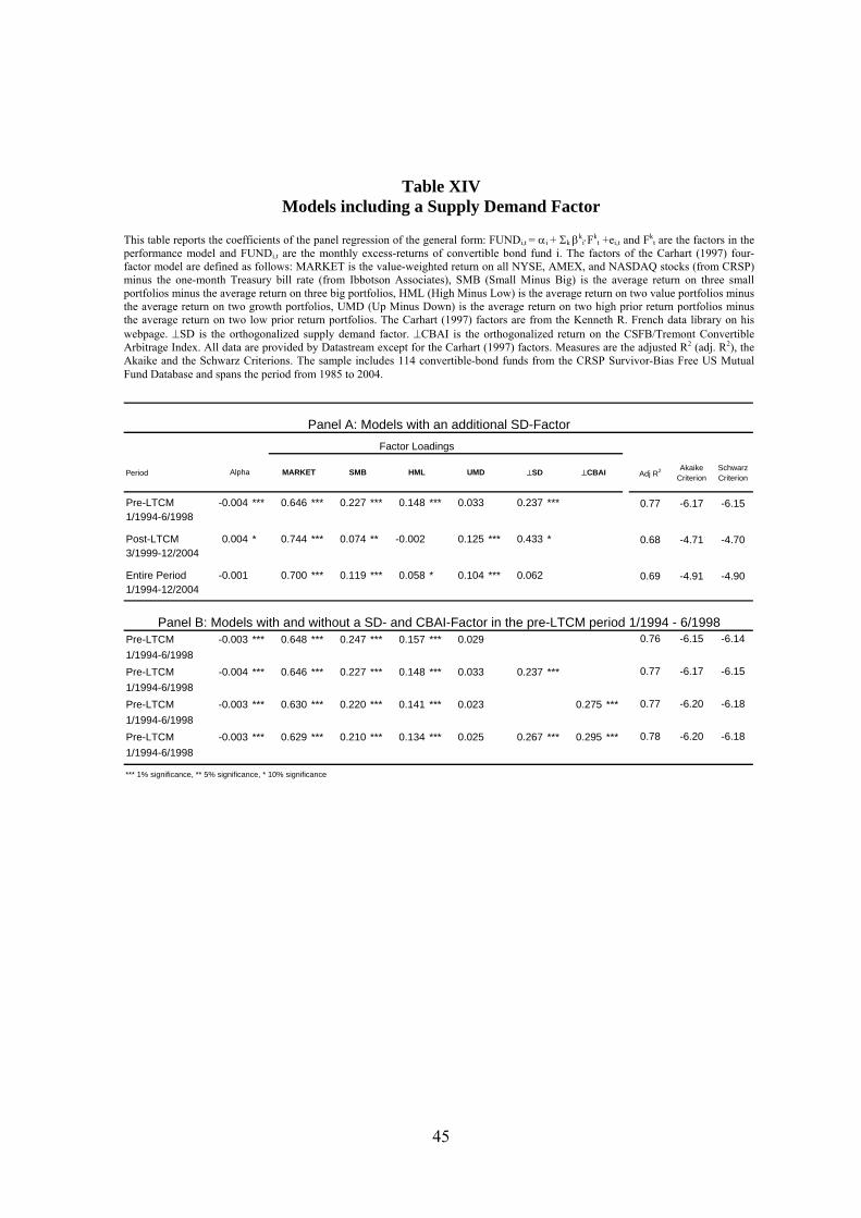
45

Table XIV Models including a Supply Demand Factor

Period Adj R2 Akaike Criterion

Schwarz Criterion

Pre-LTCM -0.004 *** 0.646 *** 0.227 *** 0.148 *** 0.033 0.237 *** 0.77 -6.17 -6.151/1994-6/1998

Post-LTCM 0.004 * 0.744 *** 0.074 ** -0.002 0.125 *** 0.433 * 0.68 -4.71 -4.703/1999-12/2004

Entire Period -0.001 0.700 *** 0.119 *** 0.058 * 0.104 *** 0.062 0.69 -4.91 -4.901/1994-12/2004

Pre-LTCM -0.003 *** 0.648 *** 0.247 *** 0.157 *** 0.029 0.76 -6.15 -6.141/1994-6/1998Pre-LTCM -0.004 *** 0.646 *** 0.227 *** 0.148 *** 0.033 0.237 *** 0.77 -6.17 -6.151/1994-6/1998Pre-LTCM -0.003 *** 0.630 *** 0.220 *** 0.141 *** 0.023 0.275 *** 0.77 -6.20 -6.181/1994-6/1998Pre-LTCM -0.003 *** 0.629 *** 0.210 *** 0.134 *** 0.025 0.267 *** 0.295 *** 0.78 -6.20 -6.181/1994-6/1998


UMD ⊥SD ⊥CBAI

Panel A: Models with an additional SD-Factor

Panel B: Models with and without a SD- and CBAI-Factor in the pre-LTCM period 1/1994 - 6/1998

Alpha MARKET SMB HML

Factor Loadings


t +ei,t and Fkt are the factors in the

performance model and FUNDi,t are the monthly excess-returns of convertible bond fund i. The factors of the Carhart (1997) four-factor model are defined as follows: MARKET is the value-weighted return on all NYSE, AMEX, and NASDAQ stocks (from CRSP) minus the one-month Treasury bill rate (from Ibbotson Associates), SMB (Small Minus Big) is the average return on three small portfolios minus the average return on three big portfolios, HML (High Minus Low) is the average return on two value portfolios minus the average return on two growth portfolios, UMD (Up Minus Down) is the average return on two high prior return portfolios minus the average return on two low prior return portfolios. The Carhart (1997) factors are from the Kenneth R. French data library on his webpage. ⊥SD is the orthogonalized supply demand factor. ⊥CBAI is the orthogonalized return on the CSFB/Tremont Convertible Arbitrage Index. All data are provided by Datastream except for the Carhart (1997) factors. Measures are the adjusted R2 (adj. R2), the Akaike and the Schwarz Criterions. The sample includes 114 convertible-bond funds from the CRSP Survivor-Bias Free US Mutual Fund Database and spans the period from 1985 to 2004.

46

The results of the panel regressions in Table XIV show that the additional SD-factor is

highly significant in the pre-LTCM period. Interestingly, its inclusion does not influence

the significance level of the convertible-arbitrage factor (CBAI). Thus, the returns of CBFs

seem to be driven by trading activities similar to those performed by convertible

arbitrageurs, such as the selection of undervalued convertibles (long part) or even, for

some funds, convertible-arbitrage strategies using short stock positions (short part).

In the multivariate cross-sectional regressions (Table XV), we analyze whether the

abnormal performance of CBFs is related to specific fund characteristics. Remarkably,

once the SD-factor is taken into account, no significant relation between CBF abnormal

returns and holding-based variables can be found. Thus, most likely, the previously

obtained positive relation between funds' performance and the difference in percentage

holdings invested in convertible bonds and stocks is, to a large extent, attributable to the

investment opportunities in the convertible-bond market, as proxied by the supply and

demand factor SD.

47

Table XV Multivariate Panel Regression Evidence: Supply and Demand Factor


0.08% 0.28% *** -0.03% 0.23% 1.22% *** -4.74%(0.18%) (0.10%) (0.02%) (0.16%) (0.37%) (7.03%)

0.20% -0.31% * -0.02% 0.19% 1.17% *** -3.34%(0.19%) (0.19%) (0.02%) (0.16%) (0.37%) (7.17%)

0.05% 0.20% -0.02% 0.19% 1.14% *** -4.01%(0.24%) (0.25%) (0.02%) (0.16%) (0.37%) (7.16%)

0.02% 0.36% *** -0.03% * 0.25% 1.20% *** -5.59%(0.19%) (0.13%) (0.02%) (0.16%) (0.37%) (7.03%)

0.10% 0.16% -0.02% 0.18% 1.16% *** -3.98%(0.20%) (0.13%) (0.02%) (0.16%) (0.37%) (7.15%)

0.18% 0.03% 0.01% -0.40% 0.32% -4.98%(0.40%) (0.24%) (0.05%) (0.30%) (0.45%) (17.32%)

0.18% 0.10% 0.01% -0.41% 0.30% -5.03%(0.39%) (0.52%) (0.05%) (0.30%) (0.45%) (17.37%)

0.54% -0.76% 0.01% -0.31% 0.32% -2.51%(0.47%) (0.50%) (0.05%) (0.30%) (0.45%) (17.06%)

0.15% 0.10% 0.01% -0.39% 0.32% -5.35%(0.41%) (0.32%) (0.05%) (0.30%) (0.45%) (17.32%)

0.32% -0.30% 0.01% -0.38% 0.27% -4.59%(0.41%) (0.30%) (0.05%) (0.30%) (0.45%) (17.25%)



Panel A: Abnormal Return based on FUNDi,t=αi+βi,1MARKETt+βi,2SMBt+βi,3HMLt+βi,4UMDt+ei,t

Panel B: Abnormal Return based on FUNDi,t=αi+βi,1MARKETt+βi,2SMBt+βi,3HMLt+βi,4UMDt+βi,5⊥SDt+ei,t

This table reports the coefficients of the monthly panel and multivariate cross-sectional regression of the general form: PERFi,t=c+χ1HVi,t-1+χ2LNTNAi,t-1+χ3ACTIVEi,t-1+χ4NMGi,t-1+χ5EXPi,t-1+εi,t where HV stands for the holding-based variables: CB-S, S, B, CB and B-S. The dependent variable, PERF, measures the monthly performance (abnormal return) using two different performance models (Panel A and Panel B) based on 36 months of lagged data to determine the betas in the performance models. The abnormal returns are calculated as follows: PERFi,t=FUNDi,t-Σk βk

i,t-1 Fkt and Fk

t are the factors in the performance model. The holding-based variables are the asset compositions in percentages invested in convertible bonds (CB), stocks (S), bonds inclusive convertible bonds (B), convertible bonds minus stocks (CB-S) and bonds inclusive convertible bonds minus stocks (B-S), respectively. We denote the natural logarithm of total net assets by LNTNA, the new money growth per month by NMG and the expense ration by EXP. The variable ACTIVE is a dummy variable and is one if the convertible bond fund is active and zero otherwise. Mitigating potential endogeneity problems, we lag all explanatory variables by one month. The sample includes convertible-bond funds from the CRSP Survivor-Bias Free US Mutual Fund Database and spans the period from 1995 to 2004 - including the data used for calculating the abnormal returns. Panel-corrected standard errors (PCSE) are reported in parenthesis.

48

6 Discussion of CBF Performance

This section builds on the results of the previous sections and explicitly addresses the

magnitude of funds' performance. First, we compute Jensen's alphas for models with stock,

bond, and option factors. As reported in Table XVI, Panel A, the large majority of CBFs

display non-significant alphas (83%-93%). The average alpha is moderately positive with

values between 0.04% and 0.07% per month. Second, we analyze alphas by including a

convertible-arbitrage factor and obtain a slight increase of average alphas and in the

number of significantly positive alphas (Table XVI, Panel B and C). Thus, convertible

arbitrage has, if any, a negative impact on the returns of CBFs (including CBAI increases

the alphas on average, and demonstrates the negative impact of arbitrage related activities

on CBF absolute returns). Third, we include the SD factor capturing investment

opportunities in the convertible-bond. Interestingly, average alphas become negative (-

0.56%) and the number of significantly negative alphas increases to 41%. We interpret the

dependence of CBF returns on the supply and demand factor SD as an indicator for

changing convertible-arbitrage activity of CBFs. In times with large convertible-bond

supply, CBFs tend to implement investment strategies related to convertible arbitrage,

which increases, in this case, funds' returns. We test this market-timing hypothesis by

employing as explanatory variable the factor (CBAI)2, defined as squared returns of the

convertible-arbitrage index CBAI. As reported in Table XVII, this convertible-arbitrage

timing factor is always highly significant, indicating strong timing skills by CBF managers.

Thus, including SD or (CBAI)2 lowers the alphas on average, and demonstrates the

positive impact of timing on CBF absolute returns. This is even more surprising when

recalling that the non-linear factor, (MARKET)2, capturing conventional market timing

was not statistically significant in previous analyses (cf. Table VI). As reported in Table

XVI, Panel C, average alphas are still significantly negative when convertible-arbitrage

timing is explicitly considered by (CBAI)2.

We sum up. When compared to passive investment strategies, CBFs deliver an average

performance. This result is not very exciting, but the way how CBF obtain it is more

interesting. First, CBFs seem to implement dynamic trading strategies related to

convertible arbitrage but, overall, they are less successful than convertible-arbitrage hedge

49

funds. Second, CBFs seem to increase their convertible-arbitrage activities in phases when

this strategy performs well, i.e. when investment opportunities in the convertible-bond

market are good. This successful timing activity compensates the weak selection skills of

CBFs' portfolio managers in the stock, bond, and convertible-bond market.

50

Table XVI

Analysis of the Alphas

Models

Percentage of significantly

negative alphas (PERFi,t)

Percentage of significantly

positive alphas (PERFi,t)

Percentage of non-significant alphas

(PERFi,t)

Mean of alphas (PERFi,t)

CARHART (MARKET, SMB HML, and UMD) 9% 2% 89% 0.07%CARHART + TERM + DEFT 5% 3% 93% 0.06%CARHART + ⊥HY 5% 7% 88% 0.07%CARHART + ⊥CBI 9% 9% 83% 0.04%CARHART + TERM + DEFT + ⊥CBI 6% 5% 89% 0.06%CARHART + ⊥HY + ⊥CBI 10% 8% 83% 0.07%

CARHART + ⊥CBAI 1% 13% 85% 0.10%CARHART + TERM + DEFT + ⊥CBAI 1% 13% 86% 0.08%CARHART + ⊥HY + ⊥CBAI 3% 16% 81% 0.13%CARHART + ⊥CBI + ⊥CBAI 1% 11% 88% 0.05%CARHART + TERM + DEFT + ⊥CBI + ⊥CBAI 5% 10% 85% 0.01%CARHART + ⊥HY + ⊥CBI + ⊥CBAI 6% 9% 85% 0.09%

CARHART + ⊥SD 41% 11% 48% -0.56%CARHART + ⊥SD + ⊥CBAI 21% 19% 60% -0.12%CARHART + (CBAI)2 22% 0% 78% -0.31%

Panel A

Panel B

Panel C

This table reports the percentage of statistically significant alphas (PERF) and the mean (per month) of the alphas (PERF) for all convertible bond funds in our sample determined with the different factor models introduced before. Panel A shows the percentage of significances for the standard models, Panel B for the extended models (with a convertible arbitrage factor), and Panel C for a model with a supply and demand (SD) factor. The sample includes 114 convertible bond funds from the CRSP Survivor-Bias Free US Mutual Fund Database and spans the period from 1985 to 2004.

51

Table XVII Models including a Timing Factor

CBAI Adj R2 Akaike Criterion

Schwarz Criterion

-0.002 0.699 *** 0.122 *** 0.059 * 0.103 *** 0.062 0.69 -4.91 -4.90

-0.004 *** 0.668 *** 0.110 *** 0.012 0.110 *** 0.454 *** 0.71 -4.99 -4.98

-0.003 ** 0.703 *** 0.136 *** 0.056 * 0.111 *** 6.715 ** 0.69 -4.92 -4.91

-0.002 0.667 *** 0.102 *** 0.006 0.112 *** -0.180 0.484 *** 0.71 -4.99 -4.98

-0.006 *** 0.671 *** 0.133 *** 0.006 0.120 *** 0.480 *** 8.883 *** 0.72 -5.01 -5.00

-0.003 * 0.670 *** 0.122 *** -0.004 0.124 *** -0.271 ** 10.105 *** 0.72 -5.01 -5.00

-0.003 * 0.670 *** 0.122 *** -0.004 0.124 *** -0.271 ** 0.529 *** 10.104 *** 0.72 -5.01 -5.00

-0.003 *** 0.694 *** 0.124 *** 0.063 * 0.090 *** 1.599 *** 0.70 -4.95 -4.94


UMD SD (CBAI)2Alpha MARKET SMB HML (CBI)2


t +ei,t and Fkt are the factors in the

performance model and FUND are the monthly excess-returns of convertible bond fund i. The factors of the Carhart (1997) four-factor model are defined as follows: MARKET is the value-weight return on all NYSE, AMEX, and NASDAQ stocks (from CRSP) minus the one-month Treasury bill rate (from Ibbotson Associates), SMB (Small Minus Big) is the average return on three small portfolios minus the average return on three big portfolios, HML (High Minus Low) is the average return on two value portfolios minus the average return on two growth portfolios, UMD (Up Minus Down) is the average return on two high prior return portfolios minus the average return on two low prior return portfolios. The Carhart (1997) factors are from the Kenneth R. French data library on his webpage. SD is the supply demand factor. CBAI is the return on the CSFB/Tremont Convertible Arbitrage Index. CBI is the return on the Merrill Lynch All US Convertible Bond Index. All data are provided by Datastream except for the Carhart (1997) factors. Measures are the adjusted R2 (adj. R2), the Akaike and the Schwarz criterion. The sample includes 114 convertible bond funds from the CRSP Survivor-Bias Free US Mutual Fund Database and spans the period from 1994 to 2004.

52

7 Conclusions

This paper presents the first empirical study on convertible-bond funds (CBFs). We

examine systematic factors that affect CBF returns using a complete and survivorship-bias-

free sample of US convertible-bond funds in the period from 1985 to 2004. Risk factors

can be divided into four categories: (i) stock factors as used in Carhart (1997); (ii) bond

factors related to the term structure and credit risk; (iii) factors reflecting the option-like

nature of convertible bonds, such as the stock-market volatility and non-linear market

factors; and (iv) fund factors related to CBF trading activity.

Carhart (1997) factors capture a significant portion of CBF returns and should therefore be

included in the data-generating process. Default risk tends to be explained equally well by

a high-yield index factor and by the return difference between a long-term corporate bond

index and a long-term government bond index. The hybrid character of convertible bonds

is best captured by a convertible-bond index. Neither an implied volatility index nor other

factors related to the non-linear payoffs of convertible bonds seem to be appropriate as

explanatory variables.

We show that for a set of plausible models there is a positive relationship between the

abnormal performance of convertible-bond funds and the difference in the funds' holdings

of convertible bonds and stocks. We argue that this relationship can be explained by

trading activities related to convertible-arbitrage. Following this line of reasoning, we

extend all models by a convertible-arbitrage factor and a supply-demand factor of the

convertible-bond market proxying for investment opportunities in this market. With this set

of models, the cross-sectional relationship between funds' performance and portfolio

holdings disappears. The results are found to be robust with respect to alternative risk

adjustments and time periods.

Building on the above insights, we assess the performance of convertible-bond funds and

draw the following conclusions. First, CBFs seem to implement dynamic trading strategies

related to convertible arbitrage but, overall, they are less successful than convertible-

53

arbitrage hedge funds. Second, CBFs seem to increase their convertible-arbitrage activities

in phases when this strategy performs well, i.e. when investment opportunities in the

convertible-bond market are good (convertible-arbitrage timing). This successful timing

activity compensates but does not overcompensate the weak selection skills of CBFs'

portfolio managers in the stock, bond, and convertible-bond market.

54

8 References

Agarwal, V. and Naik, N.Y., 2004, Risks and Portfolio Decisions Involving Hedge Funds, Review of Financial Studies 17, 63-98

Agarwal, V., W.H. Fung, Y.C. Loon and N.Y. Naik, 2006, Risk and Return in Convertible Arbitrage: Evidence from the Convertible Bond Market, Working Paper Georgia State University and London Business School.

Ammann, M., Kind A., and C. Wilde, 2003, Are convertible bonds underpriced? An analysis of the French market, Journal of Banking and Finance 27, 87-105

Ang, A., and J. Chen, 2005, CAPM over the long run: 1926-2001, NBER Working Paper 1190 Arshanapalli B., F. Fabozzi, L. N. Switzer and G. Gosselin, 2004, New Evidence on the market impact of convertible bond issues in the US, Working Paper, Concordia University, Montreal. Beck, N., and J. N. Katz, 1995, What to do (and not to do) with time-series cross-section data, American Political Science Review 89(3), 634–647 Berk, J., R. C. Green, and V. Naik, 1999, Optimal investment, growth options, and security returns, Journal of Finance , October, 1553-1607 Blake, C.R., Elton E.J., and M.J. Gruber, 1993, The Performance of Bond Mutual Funds, Journal of Business 66(3), 371-403

Burmeister, E. and Wall, K., 1986, The arbitrage pricing theory and macroeconomic factor measures, The Financial Review 21, 1–20

Carayannopoulos, P., and Kalimipalli, M., 2003, Convertible bond prices and inherent biases, Journal of Fixed Income 13, 64-73

Carhart, M., 1997, On Persistence in Mutual Fund Performance, Journal of Finance 52(1), 57-82

Chen, N., Roll, R., and S. A. Ross, 1986, Economic forces and the stock market, Journal of Business 59, 383-403

Detzler, M.L., 1999, The Performance of global bind mutual funds, Journal of Banking and Finance 23, 1195-1217

Elton, E.J., Gruber M.J. and Blake C.R., 1995, Fundamental Economic Variables, Expected Returns, and Bond Fund Performance, Journal of Finance 50(4), 1229-1256

Elton, E.J., Gruber M.J. and Blake C.R., 1999, Common Factors in Active and Passive Portfolios, European Finance Review 3, 53-78

Elton, E.J., Gruber M.J. and Blake C.R., 2003, Incentive Fees and Mutual Funds, Journal of Finance 58(2), 779-804

55

Evans, N., 2002, Is the game over for hedge funds?, Euromoney.

Fama, E.F., and French K.R., 1989, Business Conditions and Expected Returns on Stocks and Bonds, Journal of Financial Economics 25, 23-49

Fama, E.F., and French K.R., 1992, The cross-section of expected stock returns, Journal of Finance 47, 427-465

Fama, E.F., and French K.R., 1993, Common risk factors in the return on stocks and bonds, Journal of Financial Economics 33, 3-56

Ferson, W., and R. Schadt, 1996, Measuring fund strategy and performance in changing economic conditions, Journal of Finance 51(2), 425–462

Fung, W., and D. A. Hsieh, 2004a, “Hedge Fund Benchmarks: A Risk Based Approach,” Financial Analysts Journal, 60, 65-80 Fung, W., Hsieh, D.A., Naik, N.Y., and T. Ramadorai, 2005, “Hedge Funds: Performance, Risk, and Capital Formation,” Working Paper, Duke University, London Business School and University of Oxford Lummer, S.L. and M.W. Riepe, 1993, Convertible bonds as an asset class; 1957-1992, Journal of Fixed Income, 3(2), 1993

Harvey, C.R., 2001, The specification of conditional expectations. Journal of Empirical Finance 8, 573-638

Henriksson, R., and R. Merton, 1981, On market timing and investment performance, Journal of Business 54, 513–33

Jagannathan, R., and Z. Wang, 1996, The conditional CAPM and the cross-section of expected returns, Journal of Finance 51, 3–53

Kacperczyk, M., Sialm C. and L. Zheng, 2005, On the Industry Concentration of Actively Managed Equity Mutual Funds, Journal of Finance 60(4), 1984-2011

King, R., 1986, Convertible bond valuation: An empirical test, Journal of Financial Research 9 (1), 53-69

Lettau, M., and S. Ludwigson, 2001, Resurrecting the (C)CAPM: a cross-sectional test whet rink premia are time-varying, Journal of Political Economy 109, 1238–1287 Lewellen, J. and S. Nagel, 2003, The conditional CAPM does not explain asset-pricing anomalies, Manuscript, MIT Merton, R. C., 1973, An intertemporal capital asset pricing model, Econometrica 41, 867-887

Newey, W.K., and K.D. West, 1987, A simple positive definite Heteroskedasticity and Autocorrelation consistent Covariance Matrix, Econometrica 55, 703-708

56

Sirri, E., and P. Tufano, 1992, Buying and selling mutual funds: Flows, performance, fees and service, Working Paper, Harvard University. Treynor, J., and K. Mazuy, 1966, Can mutual funds outguess the market? Harvard Business Review 44,131–36

Treynor, J. L., and F. Black, 1973, How to use security analysis to improve portfolio selection, Journal of Business 46, 66–86

57

Appendix: Risk Factors and Explanatory Variables

Table A, Panel A presents the time-series variables used as factors of the data-generating

processes employed in this study. Table A, Panel B refers to the cross-sectional variables.

Monthly time-series are obtained from Datastream and the Kenneth R. French Data

Library14. The cross-sectional explanatory variables are from CRSP. Table B reports the

correlations among the cross-sectional (Panel A) and time-series (Panel B) explanatory

variables. In order to cope with the problem of multicollinearity, some variables are

orthogonalized before being used as regressors.

14 Kenneth French’s Web site: http://mba.tuck.dartmouth.edu/pages/faculty/ken.french/data_library.html

58

Table A Description of Explanatory Variables

Parameter Definition Datasource Start Date End Date

MARKET Value-weight return on all NYSE, AMEX, and NASDAQ stocks (from CRSP) minus the one-month Treasury bill rate (from Ibbotson Associates)

Kenneth R. French - Data Library 1985 2004

SMB SMB (Small Minus Big) is the average return on three small portfolios minus the average return on three big portfolios Kenneth R. French - Data Library 1985 2004

HML HML (High Minus Low) is the average return on two value portfolios minus the average return on two growth portfolios Kenneth R. French - Data Library 1985 2004

UMD UMD (Up Minus Down) is the average return on two high prior return portfolios minus the average return on two low prior return portfolios


TERM Return of the Lehman US Government Long Bond Index minus the one-month Treasury bill rate (from Ibbotson Associates) Datastream/Kenneth R. French - Data Library

1985 2004

DEFT Return on the Lehman US Corporate Long Bond Index minus the return of the Lehman US Government Long Bond Index Datastream 1985 2004

BOND Return on the Lehman US aggregated Government/Credit Bond Index minus one-month Treasury bill rate (from Ibbotson Associates)

Datastream/Kenneth R. French - Data Library

1985 2004

HY Return on the Merrill Lynch US High Yield Index Datastream 1985 2004

VOLA Return on the CBOE Volatility VXO Index Datastream 1986 2004

NL1The maximum of zero and the value-weight return on all NYSE, AMEX, and NASDAQ stocks (from CRSP) minus the return on the Lehman US aggregated Government/Credit Bond Index (=max(0,RM-RB))

Kenneth R. French - Data Library/Datastream

1985 2004

NL2Value-weight return on all NYSE, AMEX, and NASDAQ stocks (from CRSP) minus the one-month Treasury bill rate (from Ibbotson Associates) squared (=(RM-RF)2)


CBI Return on the Merrill Lynch All US Convertible Bond Index Datastream 1988 2004

CBAI Return on the CSFB/Tremont Convertible Arbitrage Index Datastream 1994 2004

FUND Monthly CBF excess-return CRSP 1985 2004

TNA The Total Net Assets (TNA) is the closing market value of securities owned, plus all assets, minus all liabilities (TNAs are reported in millions of dollars)

CRSP 1985 2004

EXP Expense Ratio is the percentage of the total investment that shareholderspay for the mutual fund’s operating expenses

CRSP 1987 2004

CB The Percentage Invested in Convertible Bonds CRSP 1995 2004

S The Percentage Invested in Common Stocks CRSP 1995 2004

B The Percentage Invested in Bonds is the percentage of thefund invested in preferred, corporate, municipal, government, and convertible bonds

CRSP 1995 2004

Panel B: Cross-Sectional Input Parameters

Panel A: Time-Series Input Parameters

This table describes the explanatory variables in this study (Panel A time-series variables and Panel B cross-sectional variables). The monthly time-series data are provided by Datastream or the Kenneth R. French Data Library. The cross-sectional explanatory variables are provided by the CRSP Survivorship Bias Free US Mutual Fund Database. Fund characteristics (EXP, CB, S, and B) are provided yearly or even more often, all other variables are provided monthly.

59

Table B Correlation Matrices

CB-S S B CB B-S LNTNA ACTIVE NMG EXP

CB-S 1.00

S -0.62 1.00

B 0.45 -0.48 1.00

CB 0.87 -0.16 0.28 1.00

B-S 0.67 -0.87 0.85 0.31 1.00

LNTNA 0.03 -0.05 0.01 0.00 0.01 1.00

ACTIVE -0.06 -0.06 0.17 -0.12 0.09 0.34 1.00

NMG -0.07 0.06 -0.02 -0.05 -0.04 -0.06 0.01 1.00

EXP 0.03 0.04 0.07 0.07 0.03 -0.25 -0.01 0.08 1.00

MARKET SMB HML UMD TERM DEFT BOND HY VOLA NL1 NL2 CBI CBAI

MARKET 1.00

SMB 0.12 1.00

HML -0.46 -0.44 1.00

UMD -0.09 -0.20 0.13 1.00

TERM 0.11 -0.21 0.08 0.11 1.00

DEFT 0.17 0.28 -0.11 -0.26 -0.65 1.00

BOND 0.12 -0.21 0.09 0.09 0.96 -0.52 1.00

HY 0.57 0.24 -0.19 -0.24 0.21 0.28 0.26 1.00

VOLA -0.53 -0.15 0.16 0.11 0.07 -0.20 0.06 -0.29 1.00NL1 0.77 0.10 -0.44 -0.11 -0.16 0.24 -0.15 0.31 -0.34 1.00NL2 -0.34 -0.20 0.09 -0.07 0.16 -0.19 0.15 -0.27 0.42 0.15 1.00

CBI 0.78 0.25 -0.41 -0.10 0.04 0.31 0.07 0.53 -0.43 0.67 -0.15 1.00

CBAI 0.14 -0.03 0.13 -0.04 0.10 0.20 0.12 0.35 0.07 0.04 -0.19 0.29 1.00

Panel B: Correlation-matrix of time-series data

Panel A: Correlation-matrix of cross-sectional data

This table reports the correlations for the cross-sectional (Panel A) and time-series (Panel B) explanatory variables. In the cross-sectional analysis, some variables have been tested separately due to their multicollinearity. In the time-series analysis, some variables have been orthogonalized due to their high correlations. The holding-based variables are the asset compositions in percentages invested in convertible bonds (CB), stocks (S), bonds inclusive convertible bonds (B), convertible bonds minus stocks (CB-S) and bonds inclusive convertible bonds minus stocks (B-S), respectively. We denote the natural logarithm of total net assets by LNTNA, the new money growth per month by NMG and the expense ration by EXP. The variable ACTIVE is a dummy variable that is one if the convertible bond fund is active and zero otherwise. All holding-based variables are provided by CRSP. MARKET is the value-weighted return on all NYSE, AMEX, and NASDAQ stocks (from CRSP) minus the one-month Treasury bill rate (from Ibbotson Associates), SMB (Small Minus Big) is the average return on three small portfolios minus the average return on three big portfolios, HML (High Minus Low) is the average return on two value portfolios minus the average return on two growth portfolios, UMD (Up Minus Down) is the average return on two high prior return portfolios minus the average return on two low prior return portfolios. TERM is the return of the Lehman US Government Long Bond Index minus the one-month Treasury bill rate. DEFT is the return on the Lehman US Corporate Long Bond Index minus the return of the Lehman US Government Long Bond Index. BOND is the return on the Lehman US aggregated Government/Credit Bond Index minus one-month Treasury bill rate. HY is the return on the Merrill Lynch US High Yield Index. VOLA is the return on the CBOE Volatility VXO Index. NL1 is the maximum of zero and the value-weighted return on all NYSE, AMEX, and NASDAQ stocks minus the return on the Lehman US aggregated Government/Credit Bond Index (=max(0,MARKET-BOND)). NL2 is the value-weighted return on all NYSE, AMEX, and NASDAQ stocks minus the one-month Treasury bill rate squared (=MARKET2). CBI is the return on the Merrill Lynch All US Convertible Bond Index. CBAI is the return on the CSFB/Tremont Convertible Arbitrage Index. All time-series data are provided by Datastream except for the Carhart (1997) factors that are from the Kenneth R. French data library on his webpage.

What Drives the Performance of Convertible-Bond Funds?

Documents

Transcript of What Drives the Performance of Convertible-Bond Funds?