the Role of Contingent Convertible Bond in Capital...

the Role of Contingent Convertible Bond

in Capital Structure Decisions

A master thesis by

Weikeng Chen [401248]MSc. Finance and International Business

Supervisor: Peter Løchte JørgensenDepartment of Economics and Business

Summer 2012Aarhus University

Business and Social Science

The Role of Contingent Convertible Bond

in Capital Structure Decisions

Weikeng ChenAarhus University

Abstract

The financial crisis has exposed flaws in the regulation of capital positionsof large financial institutions. When they get financially distressed, governmentregulators are implicitly forced to provide extensive amount of liquidity infu-sion, which usually causes a lot of public controversy. This paper develops anew derivative security, Contingent Convertible Bond, which is a debt instru-ment that automatically converts to equity if the issuing institution reaches apre-specified level of financial distress. This kind of “debt-to-equity swap” or au-tomatic bail-in is highly advantageous to the institution when it gets distressed,since raising new equity at this time has very high cost and makes it unfeasible.In this paper, we derive close-form formula for the market value of this securi-ty when the institution’s assets are modeled as a Geometric Brownian Motionprocess and its conversion trigger is set as a threshold of asset value. Our calibra-tion results show that, the introduction of Contingent Convertible Bond into thecapital structure can reduce the institution’s default probability and effectivelymitigate the management’s risk shifting motivation.

Keywords: Contingent Convertible Bond, Capital Structure, FinancialStability, Structural Model, Close-form Solution

CONTENTS i

Contents

1 Introduction 1

2 Literatures 32.1 Conversion trigger of contingent capital . . . . . . . . . . . . . . . . . 32.2 Existing research on contingent capital . . . . . . . . . . . . . . . . . . 52.3 Comparison between CoCo Bond Models with asset trigger . . . . . . 6

2.3.1 Similarities across 3 models . . . . . . . . . . . . . . . . . . . . 72.3.2 Differences across 3 models . . . . . . . . . . . . . . . . . . . . 8

3 Models 113.1 Asset Dynamics . . . . . . . . . . . . . . . . . . . . . . . . . . . . . . . 11

3.1.1 Girsanov Theorem . . . . . . . . . . . . . . . . . . . . . . . . . 113.1.2 Real World and Risk-Neutral World . . . . . . . . . . . . . . . 133.1.3 Absence of Arbitrage and Asset Equation . . . . . . . . . . . . 143.1.4 Definition of variables, functions and expectations . . . . . . . 15

3.2 Benchmark Model . . . . . . . . . . . . . . . . . . . . . . . . . . . . . 173.2.1 Security Design and Assumptions . . . . . . . . . . . . . . . . . 173.2.2 Asset Equation . . . . . . . . . . . . . . . . . . . . . . . . . . . 183.2.3 Valuation of claims . . . . . . . . . . . . . . . . . . . . . . . . . 19

3.3 Debt-Equity Model . . . . . . . . . . . . . . . . . . . . . . . . . . . . . 203.3.1 Security Design and Assumptions . . . . . . . . . . . . . . . . . 203.3.2 Asset Equation . . . . . . . . . . . . . . . . . . . . . . . . . . . 223.3.3 Valuation of claims . . . . . . . . . . . . . . . . . . . . . . . . . 22

3.4 Subordinate Debt Model . . . . . . . . . . . . . . . . . . . . . . . . . . 273.4.1 Security Design and Assumptions . . . . . . . . . . . . . . . . . 273.4.2 Asset Equation . . . . . . . . . . . . . . . . . . . . . . . . . . . 283.4.3 Valuation of claims . . . . . . . . . . . . . . . . . . . . . . . . . 29

3.5 CoCo Bond Model . . . . . . . . . . . . . . . . . . . . . . . . . . . . . 353.5.1 Security Design and Assumptions . . . . . . . . . . . . . . . . . 363.5.2 Asset Equation . . . . . . . . . . . . . . . . . . . . . . . . . . . 373.5.3 Valuation of claims . . . . . . . . . . . . . . . . . . . . . . . . . 38

4 Calibration 434.1 Default Probability . . . . . . . . . . . . . . . . . . . . . . . . . . . . . 43

4.1.1 Mathematical derivation . . . . . . . . . . . . . . . . . . . . . . 444.1.2 Calibrating the models . . . . . . . . . . . . . . . . . . . . . . . 49

4.2 Risk Shifting Motivation . . . . . . . . . . . . . . . . . . . . . . . . . . 524.2.1 Mathematical derivation . . . . . . . . . . . . . . . . . . . . . . 534.2.2 Calibrating the models . . . . . . . . . . . . . . . . . . . . . . . 55

5 Extensions 605.1 Endogenous coupon rates . . . . . . . . . . . . . . . . . . . . . . . . . 605.2 Endogenous value paid-out rate . . . . . . . . . . . . . . . . . . . . . . 62

CONTENTS ii

6 Summary 65

7 Reference 66

8 Appendix 688.1 Prove the basic properties of GBM . . . . . . . . . . . . . . . . . . . . 688.2 Derive the explicit formula of H function . . . . . . . . . . . . . . . . . 698.3 Derive an intermediate formula (40) . . . . . . . . . . . . . . . . . . . 738.4 Valuation of European call option . . . . . . . . . . . . . . . . . . . . . 748.5 Prove Equation (68) . . . . . . . . . . . . . . . . . . . . . . . . . . . . 758.6 Valuation of decompositions in Debt-Equity Model . . . . . . . . . . . 778.7 Valuation of down-and-in call barrier option . . . . . . . . . . . . . . . 788.8 Valuation of decompositions in Subordinate Debt Model . . . . . . . . 818.9 Valuation of decompositions in CoCo Bond Model . . . . . . . . . . . 82

1 INTRODUCTION 1

1 Introduction

The 2007-2009 financial crisis exposed flaws in the regulation of capital positions oflarge financial institutions (LFIs), especially big banks. The architecture governingthe financial insolvency of banks and other financial institutions needs a particularexamination. The insolvency and bankruptcy of these institutions might cause social-ly vital disruptions in the overall financial system. In order to prevent the possibleconsequence, the government regulators are forced to provide extensive amount ofimplicit guarantees when they get financially distressed, which usually take the formof outright infusion of taxpayer money to enrich their capital position. This is the socalled “Too Big To Fail” (TBTF) problem and the need for government bailout bringsa huge social cost. Facing this problem, government regulators need to put forwardsome strict proposals to improve the prudential bank regulation. However, moreimportantly, banks themselves should ensure that they have enough loss-absorbingcapital as buffer and they can internalize the losses when they get financially dis-tressed, in order to preclude a big dependence on the public bailout.To solve this problem, enhancing the bank’s financial stability by optimizing itscapital structure would be a good perspective. Some innovative and well-designedderivative securities could help to internalize the bank’s possible losses during thefinancial crisis. Among the possible choices, Contingent Convertible Bond (CoCobond, CCB), one kind of contingent capitals, would be a good derivative securitythat is potentially beneficial to the enhancement of the financial stability.Contingent Convertible Bond is a debt instrument that automatically converts toequity if the issuing bank reaches a pre-specified level of financial distress (calledconversion trigger). This derivative is issued as debt and it can enjoy the debt ben-efit of tax deduction before conversion. When a distress-related trigger is breached(usually due to the depletion of capital during a financial crisis), CoCo bond willmandatorily convert into common equity to enrich its capital position. This kind of“debt-to-equity swap” or automatic bail-in is highly advantageous to the bank whenit gets distressed, because raising new equity to enrich its capital position, anotherbail-in procedure instead, has very high cost in distress times and makes it unfeasible.So CoCo bond can be viewed as another type of capital buffer for big banks withdefault risk. It precludes the need of external government bail-out, which usuallycauses a lot of public controversy.This innovative derivative security was proposed by Flannery (2005) and the follow-ing researches extend the analysis and construct financial models for quantitativevaluation. However, regarding CoCo bond’s conversion design, equilibrium pricingand possible influence on bank’s capital structure, it still remains at an early researchstage and seems far from reaching a consensus. There are already some attempts inreal financial world. For example, Lloyd’s bank issued the first £7 billion ($11.6 bil-lion) CoCo bonds in 2009. However, as a newly emerging security, the number of realworld cases is very limited and thus the real world data is far from sufficient to testthe theoretical model. Facing this kind of data restriction, usually researchers willcalibrate the model with some well approximated parameters to see its application

1 INTRODUCTION 2

in the capital structure decision, which is also what we conduct in our empirical partafter introducing the models.Undoubtedly, different designs of the underlying assets and the contractual terms ofCoCo bond would lead to totally different models with different valuation methods,sometimes even with slightly different conclusions. In this paper, we construct a Co-Co Bond Model and present a close-form solution for the CoCo price and all otherbank claims (senior debt, subordinate debt, equity). It utilizes the outcomes fromsome of the existing models as well as makes some important improvements in thedesign of contractual terms. The existing research and our improvements will beexplained more in detail in Section 2.For a brief description of our CoCo Bond Model, the asset dynamics follow the com-mon Geometric Brownian Motion (GBM) process. We assume both the corporatesenior debt and CoCo bond have continuous coupon payment and finite maturity, adesign character that makes CoCo bond feasible and implementable in real financialmarket. The market values of all claims in our model have been successfully derivedwith close-form formula. Some other model elements such as dividend payment,possible bankruptcy cost, default probability, risk shifting motivation, etc. are alsocovered in this paper.The derivation of close-form formula is very important in derivative valuation. With-out explicit solutions, the common data simulation methods (such as Monte Carlosimulation) have very low efficiency in converging to the real number if the derivativeis complicatedly designed. Besides, close-form formula makes our comparative staticanalysis much easier and time-efficient.Models construction is the core of this paper. We begin from a Benchmark Model, theclassic Black-Scholes-Merton model of debt and equity valuation. The model frame-work and research methodology inspire us to construct other models, either by addinganother security into the capital structure, or by loosening some strict assumptions.Besides, conclusion from Benchmark Model, especially the equity-volatility relation-ship, is where the traditional and classical theory comes from and thus it is worthour attention.In order to see the role of CoCo bond in enhancing the financial stability, under theframework of Benchmark Model, we construct another 2 supporting models. Debt-Equity Model considers a capital structure with corporate debt and equity, the sameas Benchmark Model. However, many assumptions from the Benchmark Model havebeen loosened. This model is the template and basis for models with more securitiesin the capital structure. Its conclusion can be used to compare with our core model,CoCo Bond Model, to see whether it is beneficial to add CoCo bond into the capitalstructure. Another supporting model is Subordinate Debt Model. Also for compar-ison purpose, we construct this model with another debt instrument, subordinatedebt, which is used to directly “compete” with CoCo bond. So there are 4 modelsin total in our paper, 3 supporting models and a core model, CoCo Bond Model.Quantitative analysis by data calibration is performed for all 4 models, and the roleof CoCo bond is clearly displayed after the comparison.The rest of this paper is organized as follows. Section 2 examines the recent research

2 LITERATURES 3

findings and compares our CoCo Bond Model with models in 2 published papers.Section 3 presents our 4 models, each beginning from the security assumptions, thenthe valuation of all claims, and ending with the mathematical formulas. Section 4tests the advantage of CoCo bond quantitatively from 2 perspectives, default proba-bility and risk shifting motivation, by data calibration. Some extensions for the CoCoBond Model are provided in Section 5. It provides more choices and inspiring whendesigning CoCo bond in real world. Section 6 summarizes. Detailed calculationsleading to our valuation formulas are deferred to Appendix.

2 Literatures

2.1 Conversion trigger of contingent capital

Regarding the design of contingent capital, there exist a list of issues that need to besettled before implementation. Detailed proposals can refer to Flannery (2009) andMcDonald (2010). Here we just provide the most important design characteristic ofthe contingent capital: the setting of distress-related conversion trigger.Conversion trigger is widely discussed in the literatures of contingent capital. Typeof conversion trigger should be clearly determined no later than the issuance of con-tingent capital. When the trigger is reached, the conversion should be conductedmandatorily and automatically. Until now, it does not have a consensus regardingwhich should be chose as conversion trigger. For different considerations, there existdifferent types of triggers.We briefly list the conversion triggers that have been discussed and utilized in ex-isting literatures. We will not give a detailed explanation about the advantage anddisadvantage for each type of trigger as many papers have covered. Interested readerscan refer to the corresponding literatures for a deeper study.Conversion triggers in the current research can be classified into 3 types:

1. A systemic event which will make a big influence on the banking system as awhole, for example, the financial crisis which can be observed and measured bysome kind of market index, some big changes of banking supervision regulation,etc. Related research can refer to Kashyap, Rajan and Stein (2008).

2. The trigger related to the individual LFI. This is the most common type inliterature. This type of trigger includes the following financial indicators.

- Capital ratio of LFI. This is one of the most important risk ratios of LFI.It can take the form of either equity to debt value, or equity to assetvalue. Debt value and asset value are both unique; however we have 2choices for equity value: book value of equity and market value of equity.Accordingly, there exist both book capital ratio and market capital ratio.Their advantages and disadvantages will be analyzed more in detail below.In literature, for example, Flannery (2005) suggested a capital ratio basedon the market value of the bank’s equity. However, Glasserman and Nouri(2010) developed a model with a capital-ratio trigger based on book value.

2 LITERATURES 4

- Underlying asset value of LFI. Utilizing this trigger will make the analysistractable and remove the possibility of multiple equilibriums. Relatedresearch can refer to Raviv and Hilscher (2011) and Albul, Jaffee andTchitsyi (2010). In our paper, we also choose it as the conversion trigger.

- Share price of LFI. Obviously this is another market value indicator. Re-lated research can refer to Glasserman and Wang (2009).

3. The combination of 2 or more indicators. One example is a trigger based on thehealth of both an individual bank and the financial system, suggested by SquamLake Working Group (2009). Another example can be referred to McDonald(2010).

As above, according to which kind of equity value we use, there are 2 types of capitalratios for LFI: book capital ratio and market capital ratio. Market value of equityis based on the market price of the LFI’s stock. Book value of equity is based onregulatory accounting measures of debt and capital. It is also called regulatory value,or accounting value. In research, it will be the residual of asset value after deductingthe value of all kinds of debt.In current literatures, there are many discussions regarding the advantage and dis-advantage of using the book value or market value indicators. Since the discussionappears in many literatures, here we just list the general points in the literatureswithout detailedly pointing out their origin. Note that, the disadvantage of one typeof indicator may construct part of the reason why we may use the other type, viceversa.Using the book value indicators:

- Advantage: Existing regulatory capital requirements for LFIs are based pri-marily on book values.

- Advantage: Existing issuances of contingent capital to date all use triggersbased on regulatory values rather than market prices.

Using the market value indicators:

- Advantage: It is continuously updated with the newest information and reactssensitively to any market shock.

- Advantage: It is forward-looking and thus it can reveal any potential shock andshow the market and the investors’ expectation.

- Disadvantage: Market values could potentially be manipulated to trigger con-version.

- Disadvantage: Market value indicators may result in multiple solutions or nosolution for the market price of the contingent capital. This leads to the problemof the viability of contracts designed with market-based triggers. Sundaresanand Wang (2010) have a wonderful explanation for this point.

2 LITERATURES 5

2.2 Existing research on contingent capital

Before the model section, we provide a brief overview of the literatures on contingentcapital until now.The original proposal and idea of contingent capital was pioneered by Flannery.Flannery (2005) proposed a new financial security for LFIs, called reverse convertibledebentures. It is a form of debt that converts to equity if the institution’s capitalratio falls below a threshold. His proposal utilized a capital ratio based on the marketvalue of the bank’s equity, a feature that may cause multiple equilibriums or even noequilibrium, proved later by Sundaresan and Wang (2010). Flannery (2009) extentthis proposal and considered how it could be implemented in real financial market.In this proposal, he renamed it as Contingent Capital Certificates (CCC). Kashyap,Rajan and Stein (2008) proposed a custodial account, i.e. a “lock box” to hold bankfunds that would be released if an event, usually, one kind of crisis, happens overthe life of the policy. It would resemble an investment in a defaultable “catastro-phe” bond. The trigger is a systemic event, rather than the risk of the individualinstitution. Instead, the Squam Lake Working Group (2009) recommended a triggerthat based on the risk condition of both an individual bank and the banking systemas a whole. Glasserman and Wang (2009) studied the convertible securities designedby the US Treasury for its Capital Assistance Program. They suggested this kindof security can be viewed as a type of contingent capital in which banks hold theoption to convert preferred shares to common equity and the trigger can be set astheir share price.Other literatures regarding the design of contingent capital lead to model construc-tion and quantitative valuation. Some models can achieve close-form solution, i.e.explicit formula for the pricing of contingent capital and other banking claims, whileothers need to utilize some kinds of data simulation to do the valuation. McDonald(2010) got the value of contingent capital with a dual trigger through joint simulationof a bank’s share price and one kind of market index. Pennacchi (2010) developed astructural credit risk model of a bank that issued fixed or floating coupon bonds inthe form of contingent capital. The return on the bank’s assets is simulated to followa jump-diffusion process, and default-free interest rates are stochastic. Raviv andHilscher (2011) obtained closed-form pricing formula under the assumption that theconversion trigger is set by a threshold level of assets and both debts take the form ofzero-coupon deposit. They priced each banking claim by replicating its payoff usinga combination of different barrier options that all have closed form solution. Albul,Jaffee and Tchitsyi (2010) also used an asset-level trigger and obtained closed-formformula by assuming that all debts have infinite maturity. Glasserman and Nouri(2010) developed a model with a capital-ratio trigger based on book value of equi-ty. Different from the conversion process in other literatures, which is one-time andcomplete conversion, their model suggested a conversion mechanism that convertsjust enough contingent capital to meet the capital requirement each time a bank’scapital ratio reaches the threshold. Sundaresan and Wang (2010) proved that settingthe conversion trigger at a level of share price may lead to multiple solutions or no

2 LITERATURES 6

solution for the market price of contingent capital, raising questions about the fea-sibility of contracts designed with market-based triggers. Their research cast doubton the proposal suggested by Flannery, who recommended a capital ratio based onthe market value of the bank’s equity.Remaining researches proposed other methods to improve LFI’s capital position dur-ing a financial crisis. Those proposals usually take the form of either some guidingregulations, or suggestions of some innovative securities or security combination. Forexample, Duffie (2010) proposed the mandatory offering of new equity by banks whenthey face financial crisis and their capital position deteriorates. As opposed to theconversion of debt to equity, a mandatory rights offering provides new cash that mayreduce the risk of a liquidity crisis. Hart and Zingales (2010) designed a new, imple-mentable capital requirement for LFIs which ensures that LFIs are always solvent,while preserving some of the disciplinary effects of debt. Their mechanism requiredthat LFIs should maintain a sufficiently large equity cushion. If the CDS (Credit De-fault Swap) price goes above the threshold, the LFI regulator forces the LFI to issueequity until the CDS price moves back down. Pennacchi, Vermaelen and Wolff (2010)proposed a new security, the Call Option Enhanced Reverse Convertible (COERC).The security is a form of contingent capital, but at the same time, equity holdershave the option to buy back the shares from the bondholders at the conversion price.Compared to other forms of contingent capital proposed in the literature, the COER-C is less risky in a world where bank assets can experience sudden and large declinesin value.Among the existing literatures, our paper can be categorized into the type of litera-tures which lead to model construction and quantitative valuation. Similar to Ravivand Hilscher (2011) and Albul, Jaffee and Tchitsyi (2010), the conversion trigger inour model is also set as a threshold level of asset value. We make improvements byloosening some calculation-simplified assumptions in the above models, which makesthe security more implementable in real financial world. Our model also leads toclose-form solution for the valuation of each claim. In the next subsection, we willintroduce the similarities and differences between our model and the above 2 modelsmore in detail, from each model’s security design, the reason why they design in thisway, to the logic of mathematical derivation under each model. The comparison alsoguides the readers into our model construction gradually and implicitly explains whywe design the model in this way and its significance.

2.3 Comparison between CoCo Bond Models with asset trigger

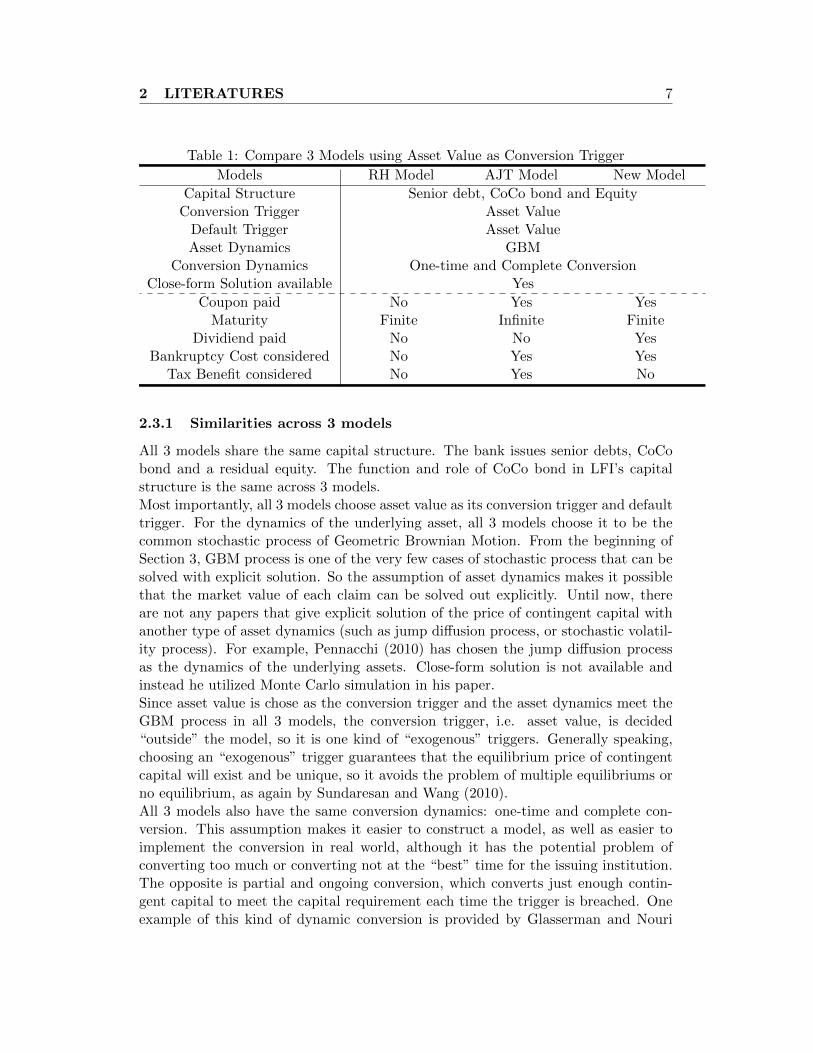
To introduce our model gradually, we describe and compare 2 CoCo Bond Modelswith our model. 3 models all choose the asset value as conversion trigger. As isexplained before, using asset value as conversion trigger makes the analysis tractableand removes the possibility of multiple equilibriums. The comparison of 3 modelscan be clearly shown in Table 1.

2 LITERATURES 7

Table 1: Compare 3 Models using Asset Value as Conversion Trigger

Models RH Model AJT Model New Model

Capital Structure Senior debt, CoCo bond and EquityConversion Trigger Asset Value

Default Trigger Asset ValueAsset Dynamics GBM

Conversion Dynamics One-time and Complete ConversionClose-form Solution available Yes

Coupon paid No Yes YesMaturity Finite Infinite Finite

Dividiend paid No No YesBankruptcy Cost considered No Yes Yes

Tax Benefit considered No Yes No

2.3.1 Similarities across 3 models

All 3 models share the same capital structure. The bank issues senior debts, CoCobond and a residual equity. The function and role of CoCo bond in LFI’s capitalstructure is the same across 3 models.Most importantly, all 3 models choose asset value as its conversion trigger and defaulttrigger. For the dynamics of the underlying asset, all 3 models choose it to be thecommon stochastic process of Geometric Brownian Motion. From the beginning ofSection 3, GBM process is one of the very few cases of stochastic process that can besolved with explicit solution. So the assumption of asset dynamics makes it possiblethat the market value of each claim can be solved out explicitly. Until now, thereare not any papers that give explicit solution of the price of contingent capital withanother type of asset dynamics (such as jump diffusion process, or stochastic volatil-ity process). For example, Pennacchi (2010) has chosen the jump diffusion processas the dynamics of the underlying assets. Close-form solution is not available andinstead he utilized Monte Carlo simulation in his paper.Since asset value is chose as the conversion trigger and the asset dynamics meet theGBM process in all 3 models, the conversion trigger, i.e. asset value, is decided“outside” the model, so it is one kind of “exogenous” triggers. Generally speaking,choosing an “exogenous” trigger guarantees that the equilibrium price of contingentcapital will exist and be unique, so it avoids the problem of multiple equilibriums orno equilibrium, as again by Sundaresan and Wang (2010).All 3 models also have the same conversion dynamics: one-time and complete con-version. This assumption makes it easier to construct a model, as well as easier toimplement the conversion in real world, although it has the potential problem ofconverting too much or converting not at the “best” time for the issuing institution.The opposite is partial and ongoing conversion, which converts just enough contin-gent capital to meet the capital requirement each time the trigger is breached. Oneexample of this kind of dynamic conversion is provided by Glasserman and Nouri

2 LITERATURES 8

(2010).Different from the attempt of “using other stochastic process than GBM process”,which makes it nearly impossible to get a close-form solution, the assumption of“partly conversion” can lead to close-form solution after a slightly more complicatedcalculation. The model by Glasserman and Nouri has successfully done it.

2.3.2 Differences across 3 models

More importantly, we need to overview the different designs across 3 models, whichshow the improvements we have made in our model. In brief, the improvement workfocuses mainly on the loosening of 2 assumptions of bond design, zero-coupon as-sumption for RH Model and infinite maturity assumption for AJT Model. Naturally,coupon payment and bond maturity will be the concentration of the following anal-ysis.

RH ModelWe call the CoCo Bond Model developed by Raviv and Hilscher (2011) as RH Modelfor short. In RH Model, the senior debt takes the form of zero-coupon deposit. Nodividend is distributed to the equity holder during the maturity. This means thatthere are no cash outflows before the maturity. If we use Expression (13) in Section3 to describe the dynamics of underlying assets under Q-measure, in this model wehave δ = 0 and the drift of the underlying assets is equal to the risk free interest rater.Without coupon payment, the only way for senior debt holder (deposit holder here)to realize value from their investment is the payment at maturity, so in this model,the maturity should be finite. Otherwise the senior debt holders get nothing if theirlife span is smaller than infinite.Without coupon payment, it is not possible to consider the tax-saving benefit. Taxbenefit takes a form of tax saving for the debt interest the banks pay out during theyear. In RH Model, banks do not pay out any coupons during the maturity, so thereis no tax benefit and thus it is not considered.In RH Model, bankruptcy cost is also not covered. This simplification does not inline with most structural models in literature, and we will make the correction in ourmodel.Because of the assumption of no coupon payment and no bankruptcy cost, the valu-ation of 3 banking claims (senior debts, CoCo bond and equity) is simplified. Theyprice each claim by replicating its payoff using a combination of different barrier op-tions that all have closed form solution. So the close-form solution of each claim iseasily calculated. Note that all the barrier options they use to replicate the bankingclaims are the type of “down” barrier option (down-and-in option or down-and-outoption), because by assuming the initial asset value larger than the conversion trig-ger, the CoCo bond will converse only when the asset value falls down and hits thetrigger.To save space, we will not list their pricing formulas here. It is easily checked in their

2 LITERATURES 9

paper.

AJT ModelWe call the CoCo Bond Model developed by Albul, Jaffee and Tchitsyi (2010) as AJTModel for short. AJT Model calls senior debt as straight bond or straight debt. It isjust a matter of denomination and its role is exactly the same as senior debt in ouranalysis. In AJT Model, both straight bond and CoCo bond are consol type, meaningthey are annuities with infinitive maturity. Straight bond pays coupon continuallyin time until default. At default, fraction α of the bank’s assets is lost. CoCo bondpays coupon continually in time until it hits the conversion trigger. The amounts ofboth coupon payments are constants and they are decided exogenously.Since both bonds pay coupon continuously in time before the maturity, it is possibleto assume that the bonds’ maturity is infinite (not necessarily though, such as ourmodel), i.e. one kind of annuities. The payoffs of both bonds are taking the formof continuously paying coupons. They have a final payment only when it defaults orconverses.Although not common in real world, this assumption also simplifies the pricing cal-culation. To calculate the present value of coupon payment, it is always easier whenthe maturity is infinite. As in Section 3, both stopping times (conversion time anddefault time) are always finite (P(τ = +∞) = 0). So when the maturity is infinite,CoCo bond will always covert before the maturity, and the bank will always defaultbefore the maturity, meaning that there is just one possibility to be considered in thevaluation. If the maturity is finite as in our model, we need to figure out differentpossibilities regarding the comparison of stopping time and maturity. The calculationof the present value of coupon payment with infinite maturity is somewhat similar towhat we calculate for the present value of the annuity (interest paid out each perioddivided by interest rate).Besides, we always need to consider the final payment when default or conversionhappens, which is a certain event because the maturity is infinite. This kind of u-nique possibility also simplifies the calculation.Because of the payment of continuous coupon, the parameter of cash outflow δ is notequal to 0 in this model, meaning that the drift of underlying assets under Q-measurewill be smaller than r (it will be r−δ). They call it µ in their paper. The exact valueof δ (and thus µ) is needed because it decides both stopping times. In AJT Model,its value is exogenously decided. In their paper, they do not consider dividend ofequity.Different from RH Model, AJT Model considers bankruptcy cost. As in the generalliterature, it is set as a constant proposition of the asset value when it hits the defaulttrigger. In their model, bankruptcy cost will always be positive because, as before,default trigger will always be reached with an infinite maturity.Besides, they also consider tax benefit in their model. As before, tax benefit is thetax deduction for paid debt interest during the year. In general literature, it is alwaysset as a constant fraction of the coupon paid out (it is the exogenously decided θ intheir paper). So the amount of tax benefit is easily got after the valuation of both

2 LITERATURES 10

coupons is calculated.From the above analysis, we can get the conclusion that, in order to get the close-form solution, both models have made some strict assumptions. In RH Model, theyassume that the senior debt takes the form of zero-coupon deposit. However, ingeneral structural models, we always assume the bonds pay coupons, continuouslyor discreetly. Actually, coupon payment is one important element of the design ofbonds and its amount will greatly affect the value of bonds. In AJT Model, eventhough coupon payment is considered, they assume that both bonds are consol type,meaning they are annuities with infinitive maturity. This simplification assumptionis also not in line with most cases of bonds in real financial world. In one word, bothdesigns make CoCo bond easier for theoretical valuation, but not implementable inreal financial market.What about a new model to loosen both assumptions, making the design of CoCobond more realistic and implementable even though the valuation may be a bit morecomplicated? This is our motivation and inspiration to design a new CoCo BondModel.

New ModelThe biggest difference in our model is the loose of some assumptions of both bonds.We assume that both bonds have continuously coupon payment, with finite maturity.The assumption is more in compliance with the general assumption of bonds inliterature, as well as the feasible design of real world bonds. So our correction willbe an improvement for the existing CoCo Bond Models which use asset level as itsconversion trigger.A positive coupon payment, different from RH Model’s zero-coupon deposit, meansthe bank will have cash outflow before the maturity. As in AJT Model, the drift ofunderlying asset under Q-measure will be smaller than r (we set it as r − δ in ourmodel).A finite maturity, different from AJT Model, means that both stopping times can beeither before or after the maturity. Now we need to consider both possibilities whenwe do the valuation for each claim.In other aspects of the model design, there also exist some differences. In AJT Model,value paid-out rate δ is decided exogenously (via µ). In the main content of thispaper, δ is exogenously decided when dividend payment is included. In the Extensionsection, δ is endogenously decided when dividend payment is not considered. Besides,regarding the amount of coupon payment, our model is slightly different from thatof AJT Model. In their model, the amounts of both coupon payments are constantsand they are decided exogenously. In our paper, coupon payment is a constantfraction (we call it coupon rate) of the face value of bond. Usually the face value ofbond is decided at the initial time when the bond is issued. So if the coupon rateis decided exogenously, the coupon design will actually be the same as AJT Model(both kinds are constant). This is the case in our main content. However, in one ofour extensions, we also consider the case of endogenously coupon rates. So at thissetting, the coupon payment is still fixed continuously across the maturity, however

3 MODELS 11

it is decided endogenously.Bankruptcy cost is also considered in our model. The setting is the same as AJTModel, which is in line with most literatures. Different from their model, we do notconsider the tax benefit. As before, this claim is easy to get because it is just aconstant fraction of the coupon payment. About the dividend payment, we take itinto consideration in our main model, but do not consider it in our Extension. Asis shown in the model section, this makes a big difference about the setting of valuepaid out rate δ.In conclusion, our models make some improvements about the design of CoCo bond(also the normal senior debt) by loosening some calculation-orientation assumptions.It makes the calculation a little more complicated, but its advantage in theoreticaldesign and practical application overwhelms. More detail of the design of our modelis provided in the model section.In the following model section, 3 supporting models are introduced before our coremodel, the CoCo Bond Model. We begin from a Benchmark Model, the classicBlack-Scholes-Merton model of debt and equity valuation. Based on the frameworkof Benchmark Model, we construct Debt-Equity Model in which many assumptionsof Benchmark Model have been loosened. Subordinate Debt Model adds subordinatedebt, another debt instrument, into the bank’s capital structure, which is used todirectly “compete” with CoCo bond in our analysis. Finally, CoCo Bond Model willbe introduced.

3 Models

3.1 Asset Dynamics

All of our models utilize standard option pricing method, which is based on a longline of research on capital structure that includes Black and Scholes (1973), Merton(1973; 1974), Black and Cox (1976), Leland (1994; 1996), and numerous subsequentpapers. This approach starts by modeling the dynamics of a firm’s assets and thenprices debt and equity as claims on those assets. We will begin with the dynamicsanalysis of the firm’s underlying assets. Before our model, we will introduce GirsanovTheorem briefly since it is frequently applied in our paper.

3.1.1 Girsanov Theorem

Let Ztt>0 be a standard Brownian motion, defined on a probability space (Ω,F ,P),and let Ftt>0 be the associated Brownian filtration. Let θtt>0 be an adapted pro-cess satisfying the hypotheses of Novikov’s Proposition:

E[exp

(∫ t

0θ2s ds

)]< +∞ ∀t > 0 (1)

Define

Mt = exp

(∫ t

0θs dZs −

1

2

∫ t

0θ2s ds

)(2)

3 MODELS 12

Now we can define a new probability measure Q on the measurable space (Ω,F) asfollows.For each T > 0 and any event F ∈ FT ,

Q(F ) = EP[MT1F

](3)

If we define

Zt = Zt −∫ t

0θs ds , t ∈ [0, T ] (4)

Under the probability measure Q, the stochastic process Zt06t6T is a standardBrownian motion.This is the famous Girsanov Theorem. It is commonly used for the transformationof probability measures in stochastic process.Now we move to a special application of Girsanov Theorem.If we set θt = θ ∈ R ∀t > 0, it simplifies to the Cameron-Martin Theorem, which isviewed as the most important special case of Girsanov Theorem.When θt = θ, the hypotheses of Novikov’s Proposition (1) is easily met. We can write(2) as:

Mt(θ) = exp

(∫ t

0θ dZs −

1

2

∫ t

0θ2 ds

)= eθZt−θ

2t/2 (5)

As before, Ztt>0 is a standard Brownian motion under the probability measure P(we also write it as P0, with the corresponding expectation operator E0). We candefine a new probability measure Q (we also write it as Pθ, with the correspondingexpectation operator Eθ) on (Ω,F) as follows.For each T > 0 and any event F ∈ FT ,

Pθ(F ) = E0

[MT (θ)1F

]or P0(F ) = Eθ

[MT (θ)−11F

](6)

For each T > 0 and any nonnegative random variable Y ,

Eθ[Y ] = E0 [MT (θ)Y ] or E0[Y ] = Eθ[MT (θ)−1Y

](7)

Similar to (4), if we define

Zt = Zt −∫ t

0θ ds = Zt − θt , t ∈ [0, T ] (8)

Under the probability measure Q = Pθ, the stochastic process Zt06t6T is a standardBrownian motion.From Cameron-Martin Theorem, we know that Zt06t6T is a Brownian motion withdrift θ under the probability measure Q = Pθ.Cameron-Martin Theorem deals only with special probability measures under whichpaths are distributed as Brownian motion with constant drift. However, GirsanovTheorem applies to nearly all probability measures. For the mathematical derivationin this paper, we need to transform the Brownian motion (with or without drift) underP-measure into another Brownian motion (with or without drift) under Q-measure.So Cameron-Martin Theorem is well enough for our calculation.

3 MODELS 13

3.1.2 Real World and Risk-Neutral World

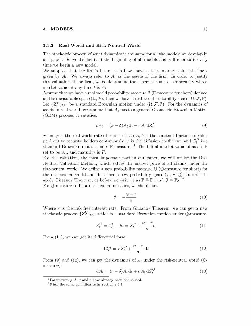
The stochastic process of asset dynamics is the same for all the models we develop inour paper. So we display it at the beginning of all models and will refer to it everytime we begin a new model.We suppose that the firm’s future cash flows have a total market value at time tgiven by At. We always refer to At as the assets of the firm. In order to justifythis valuation of the firm, we could assume that there is some other security whosemarket value at any time t is At.Assume that we have a real world probability measure P (P-measure for short) definedon the measurable space (Ω,F), then we have a real world probability space (Ω,F ,P).Let ZPt t>0 be a standard Brownian motion under (Ω,F ,P). For the dynamics ofassets in real world, we assume that At meets a general Geometric Brownian Motion(GBM) process. It satisfies:

dAt = (ϕ− δ)At dt+ σAt dZPt (9)

where ϕ is the real world rate of return of assets, δ is the constant fraction of valuepaid out to security holders continuously, σ is the diffusion coefficient, and ZPt is astandard Brownian motion under P-measure. 1 The initial market value of assets isset to be A0, and maturity is T .For the valuation, the most important part in our paper, we will utilize the RiskNeutral Valuation Method, which values the market price of all claims under therisk-neutral world. We define a new probability measure Q (Q-measure for short) forthe risk neutral world and thus have a new probability space (Ω,F ,Q). In order toapply Girsanov Theorem, as before we write it as P , P0 and Q , Pθ. 2

For Q-measure to be a risk-neutral measure, we should set

θ = −ϕ− rσ

(10)

Where r is the risk free interest rate. From Girsanov Theorem, we can get a newstochastic process ZQt t>0 which is a standard Brownian motion under Q-measure.

ZQt = ZPt − θt = ZPt +ϕ− rσ

t (11)

From (11), we can get its differential form:

dZQt = dZPt +ϕ− rσ

dt (12)

From (9) and (12), we can get the dynamics of At under the risk-neutral world (Q-measure):

dAt = (r − δ)At dt+ σAt dZQt (13)

1Parameters ϕ, δ, σ and r have already been annualized.2θ has the same definition as in Section 3.1.1.

3 MODELS 14

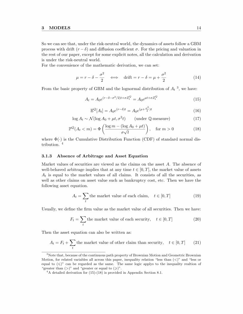
So we can see that, under the risk-neutral world, the dynamics of assets follow a GBMprocess with drift (r− δ) and diffusion coefficient σ. For the pricing and valuation inthe rest of our paper, except for some explicit notes, all the calculation and derivationis under the risk-neutral world.For the convenience of the mathematic derivation, we can set:

µ = r − δ − σ2

2⇐⇒ drift = r − δ = µ+

σ2

2(14)

From the basic property of GBM and the lognormal distribution of At3, we have:

At = A0e(r−δ−σ2/2)t+σZQt = A0e

µt+σZQt (15)

EQ[At] = A0e(r−δ)t = A0e

(µ+σ2

2)t (16)

logAt ∼ N (logA0 + µt, σ2t) (under Q-measure) (17)

PQ(At < m) = Φ

(logm− (logA0 + µt)

σ√t

), for m > 0 (18)

where Φ(·) is the Cumulative Distribution Function (CDF) of standard normal dis-tribution. 4

3.1.3 Absence of Arbitrage and Asset Equation

Market values of securities are viewed as the claims on the asset A. The absence ofwell-behaved arbitrage implies that at any time t ∈ [0, T ], the market value of assetsAt is equal to the market values of all claims. It consists of all the securities, aswell as other claims on asset value such as bankruptcy cost, etc. Then we have thefollowing asset equation.

At =∑t

the market value of each claim, t ∈ [0, T ] (19)

Usually, we define the firm value as the market value of all securities. Then we have:

Ft =∑t

the market value of each security, t ∈ [0, T ] (20)

Then the asset equation can also be written as:

At = Ft +∑t

the market value of other claim than security, t ∈ [0, T ] (21)

3Note that, because of the continuous path property of Brownian Motion and Geometric BrownianMotion, for related variables all across this paper, inequality relation “less than (<)” and “less orequal to (6)” can be regarded as the same. The same logic applys to the inequality realtion of“greater than (>)” and “greater or equal to (>)”.

4A detailed derivation for (15)-(18) is provided in Appendix Section 8.1.

3 MODELS 15

Especially, at time t = 0, the sum of the initial market value of all claims is equal tothe initial asset value A0.Asset Equation is the most important equality relationship in our paper. It will beverified in every model we develop. The fulfillment of asset equation guarantees thatour models are internally consistent. Besides, it can also be used to verify whetherour close-form solution is correctly derived.

3.1.4 Definition of variables, functions and expectations

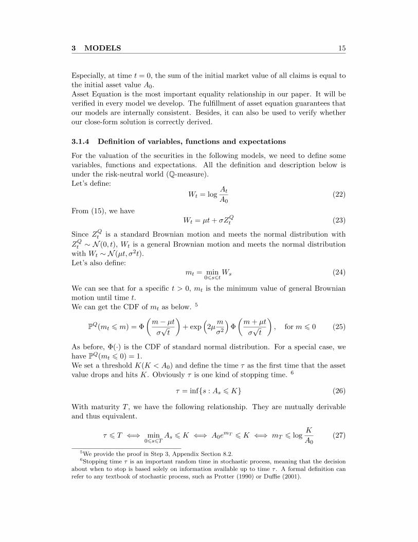
For the valuation of the securities in the following models, we need to define somevariables, functions and expectations. All the definition and description below isunder the risk-neutral world (Q-measure).Let’s define:

Wt = logAtA0

(22)

From (15), we haveWt = µt+ σZQt (23)

Since ZQt is a standard Brownian motion and meets the normal distribution with

ZQt ∼ N (0, t), Wt is a general Brownian motion and meets the normal distributionwith Wt ∼ N (µt, σ2t).Let’s also define:

mt = min06s6t

Ws (24)

We can see that for a specific t > 0, mt is the minimum value of general Brownianmotion until time t.We can get the CDF of mt as below. 5

PQ(mt 6 m) = Φ

(m− µtσ√t

)+ exp

(2µm

σ2

)Φ

(m+ µt

σ√t

), for m 6 0 (25)

As before, Φ(·) is the CDF of standard normal distribution. For a special case, wehave PQ(mt 6 0) = 1.We set a threshold K(K < A0) and define the time τ as the first time that the assetvalue drops and hits K. Obviously τ is one kind of stopping time. 6

τ = infs : As 6 K (26)

With maturity T , we have the following relationship. They are mutually derivableand thus equivalent.

τ 6 T ⇐⇒ min06s6T

As 6 K ⇐⇒ A0emT 6 K ⇐⇒ mT 6 log

K

A0(27)

5We provide the proof in Step 3, Appendix Section 8.2.6Stopping time τ is an important random time in stochastic process, meaning that the decision

about when to stop is based solely on information available up to time τ . A formal definition canrefer to any textbook of stochastic process, such as Protter (1990) or Duffie (2001).

3 MODELS 16

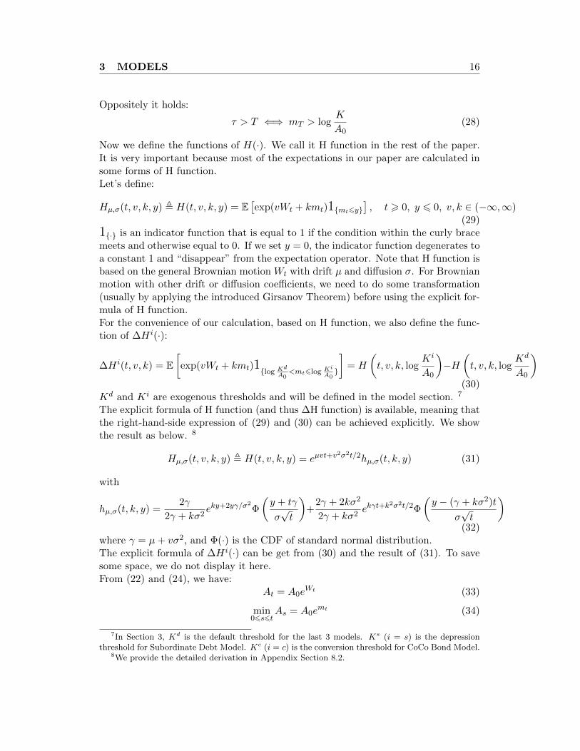
Oppositely it holds:

τ > T ⇐⇒ mT > logK

A0(28)

Now we define the functions of H(·). We call it H function in the rest of the paper.It is very important because most of the expectations in our paper are calculated insome forms of H function.Let’s define:

Hµ,σ(t, v, k, y) , H(t, v, k, y) = E[exp(vWt + kmt)1mt6y

], t > 0, y 6 0, v, k ∈ (−∞,∞)

(29)1· is an indicator function that is equal to 1 if the condition within the curly bracemeets and otherwise equal to 0. If we set y = 0, the indicator function degenerates toa constant 1 and “disappear” from the expectation operator. Note that H function isbased on the general Brownian motion Wt with drift µ and diffusion σ. For Brownianmotion with other drift or diffusion coefficients, we need to do some transformation(usually by applying the introduced Girsanov Theorem) before using the explicit for-mula of H function.For the convenience of our calculation, based on H function, we also define the func-tion of ∆H i(·):

∆H i(t, v, k) = E[exp(vWt + kmt)1log Kd

A0<mt6log K

i

A0

]= H

(t, v, k, log

Ki

A0

)−H

(t, v, k, log

Kd

A0

)(30)

Kd and Ki are exogenous thresholds and will be defined in the model section. 7

The explicit formula of H function (and thus ∆H function) is available, meaning thatthe right-hand-side expression of (29) and (30) can be achieved explicitly. We showthe result as below. 8

Hµ,σ(t, v, k, y) , H(t, v, k, y) = eµvt+v2σ2t/2hµ,σ(t, k, y) (31)

with

hµ,σ(t, k, y) =2γ

2γ + kσ2eky+2yγ/σ2

Φ

(y + tγ

σ√t

)+

2γ + 2kσ2

2γ + kσ2ekγt+k

2σ2t/2Φ

(y − (γ + kσ2)t

σ√t

)(32)

where γ = µ+ vσ2, and Φ(·) is the CDF of standard normal distribution.The explicit formula of ∆H i(·) can be get from (30) and the result of (31). To savesome space, we do not display it here.From (22) and (24), we have:

At = A0eWt (33)

min06s6t

As = A0emt (34)

7In Section 3, Kd is the default threshold for the last 3 models. Ks (i = s) is the depressionthreshold for Subordinate Debt Model. Kc (i = c) is the conversion threshold for CoCo Bond Model.

8We provide the detailed derivation in Appendix Section 8.2.

3 MODELS 17

mt 6 y ⇐⇒ min06s6t

As 6 A0ey (35)

After some transformation, we can rewrite H(·) and ∆H i(·) as:

H(t, v, k, y) = E

(AtA0

)v ( min06s6t

As

A0

)k1min

06s6tAs 6 A0e

y

(36)

∆H i(t, v, k) = E

(AtA0

)v ( min06s6t

As

A0

)k1Kd < min

06s6tAs 6 Ki

(37)

With the threshold K and stopping time τ defined in (26), it is easy to get thefollowing risk-neutral probabilities:

PQ(τ 6 T ) = P(mT 6 log

K

A0

)= E

[1mT6log K

A0

]= H

(T, 0, 0, log

K

A0

)(38)

PQ(τ > T ) = P(mT > log

K

A0

)= 1− E

[1mT6log K

A0

]= 1−H

(T, 0, 0, log

K

A0

)(39)

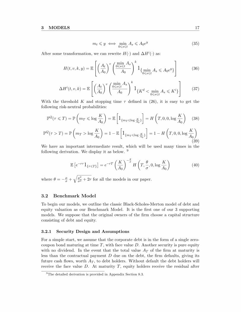
We have an important intermediate result, which will be used many times in thefollowing derivation. We display it as below. 9

E[e−rτ1τ6T

]= e−rT

(K

A0

)− θσ

H

(T,θ

σ, 0, log

K

A0

)(40)

where θ = −µσ +

√µ2

σ2 + 2r for all the models in our paper.

3.2 Benchmark Model

To begin our models, we outline the classic Black-Scholes-Merton model of debt andequity valuation as our Benchmark Model. It is the first one of our 3 supportingmodels. We suppose that the original owners of the firm choose a capital structureconsisting of debt and equity.

3.2.1 Security Design and Assumptions

For a simple start, we assume that the corporate debt is in the form of a single zero-coupon bond maturing at time T , with face value D. Another security is pure equitywith no dividend. In the event that the total value AT of the firm at maturity isless than the contractual payment D due on the debt, the firm defaults, giving itsfuture cash flows, worth AT , to debt holders. Without default the debt holders willreceive the face value D. At maturity T , equity holders receive the residual after

9The detailed derivation is provided in Appendix Section 8.3.

3 MODELS 18

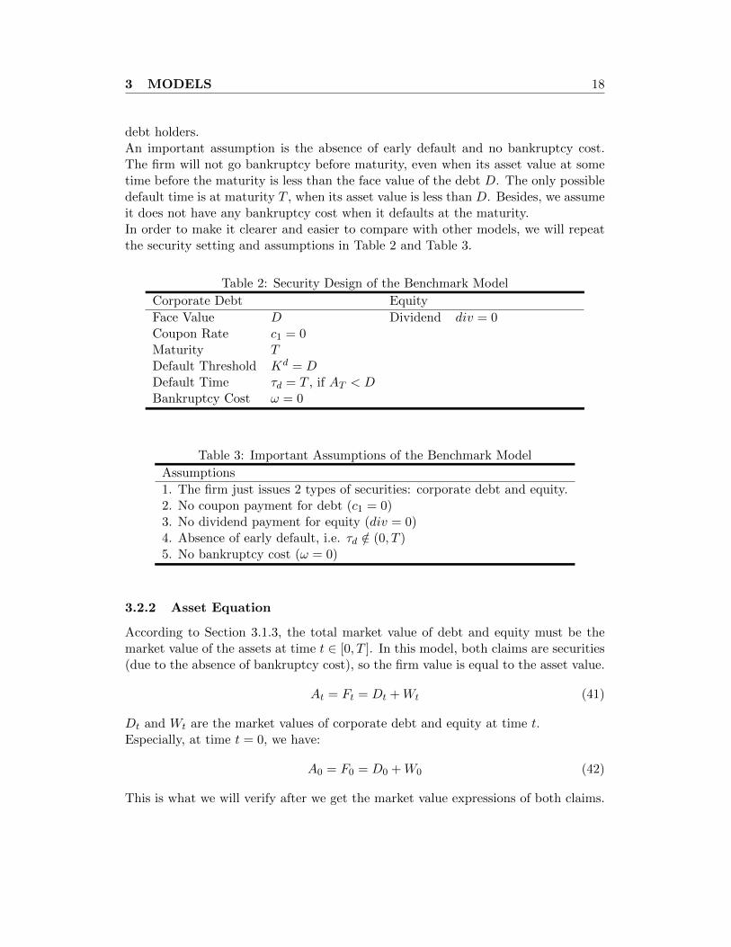
debt holders.An important assumption is the absence of early default and no bankruptcy cost.The firm will not go bankruptcy before maturity, even when its asset value at sometime before the maturity is less than the face value of the debt D. The only possibledefault time is at maturity T , when its asset value is less than D. Besides, we assumeit does not have any bankruptcy cost when it defaults at the maturity.In order to make it clearer and easier to compare with other models, we will repeatthe security setting and assumptions in Table 2 and Table 3.

Table 2: Security Design of the Benchmark Model

Corporate Debt Equity

Face Value D Dividend div = 0Coupon Rate c1 = 0Maturity TDefault Threshold Kd = DDefault Time τd = T , if AT < DBankruptcy Cost ω = 0

Table 3: Important Assumptions of the Benchmark Model

Assumptions

1. The firm just issues 2 types of securities: corporate debt and equity.2. No coupon payment for debt (c1 = 0)3. No dividend payment for equity (div = 0)4. Absence of early default, i.e. τd /∈ (0, T )5. No bankruptcy cost (ω = 0)

3.2.2 Asset Equation

According to Section 3.1.3, the total market value of debt and equity must be themarket value of the assets at time t ∈ [0, T ]. In this model, both claims are securities(due to the absence of bankruptcy cost), so the firm value is equal to the asset value.

At = Ft = Dt +Wt (41)

Dt and Wt are the market values of corporate debt and equity at time t.Especially, at time t = 0, we have:

A0 = F0 = D0 +W0 (42)

This is what we will verify after we get the market value expressions of both claims.

3 MODELS 19

3.2.3 Valuation of claims

As described in Section 3.1.2, the market values of both claims are calculated underthe risk-neutral world. In order to conduct the valuation in a clear way, we make itinto 4 steps. The analysis by steps will apply across all 4 models.

Valuation FormulaIn this model, since there are no distribution of values before the maturity (neithercoupon nor dividend), the parameter of value paid-out rate δ = 0.For debt holders, at maturity, they will receive the face value D if the firm does notdefault. Otherwise they will take over the firm and receive AT . There is not anycoupon payment. So the market value of debt at time t = 0 is:

D0 = EQ[e−rT min(AT , D)

](43)

For equity holders, they will receive the residual at maturity. There is not anydividend payment. So the market value of equity at time t = 0 is:

W0 = EQ[e−rT max(AT −D, 0)

](44)

Verify Asset EquationWe can easily verify the Asset Equation (42) in this model.

D0 +W0 = e−rTEQ [min(AT , D) + max(AT −D, 0)]

= e−rTEQ [D + min(AT −D, 0) + max(AT −D, 0)]

= e−rTEQ [D + (AT −D) + 0]

= e−rTEQ [AT ]

= A0 (45)

(16) is used when we calculate the expectation of AT .

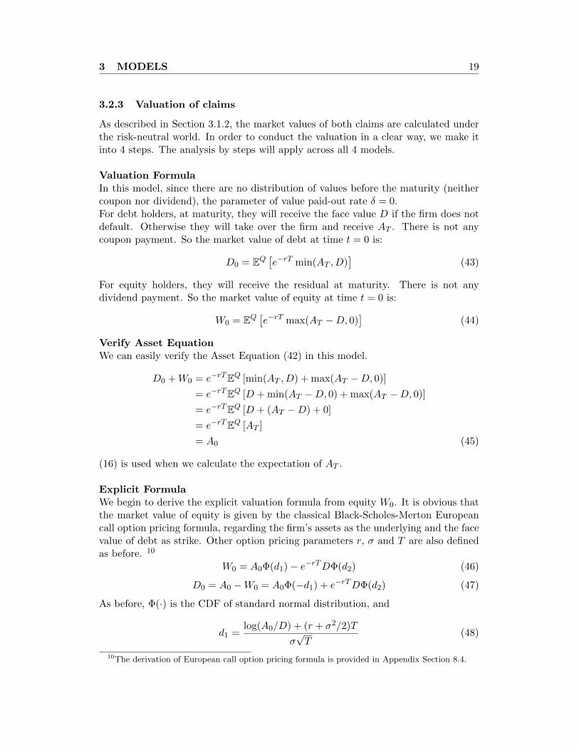
Explicit FormulaWe begin to derive the explicit valuation formula from equity W0. It is obvious thatthe market value of equity is given by the classical Black-Scholes-Merton Europeancall option pricing formula, regarding the firm’s assets as the underlying and the facevalue of debt as strike. Other option pricing parameters r, σ and T are also definedas before. 10

W0 = A0Φ(d1)− e−rTDΦ(d2) (46)

D0 = A0 −W0 = A0Φ(−d1) + e−rTDΦ(d2) (47)

As before, Φ(·) is the CDF of standard normal distribution, and

d1 =log(A0/D) + (r + σ2/2)T

σ√T

(48)

10The derivation of European call option pricing formula is provided in Appendix Section 8.4.

3 MODELS 20

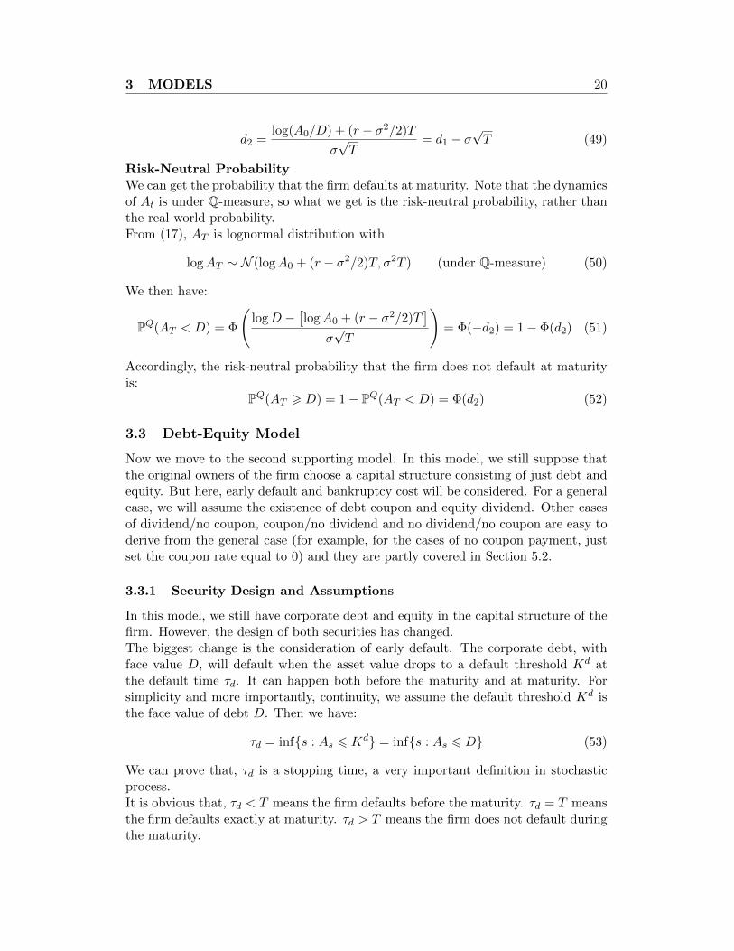
d2 =log(A0/D) + (r − σ2/2)T

σ√T

= d1 − σ√T (49)

Risk-Neutral ProbabilityWe can get the probability that the firm defaults at maturity. Note that the dynamicsof At is under Q-measure, so what we get is the risk-neutral probability, rather thanthe real world probability.From (17), AT is lognormal distribution with

logAT ∼ N (logA0 + (r − σ2/2)T, σ2T ) (under Q-measure) (50)

We then have:

PQ(AT < D) = Φ

(logD −

[logA0 + (r − σ2/2)T

]σ√T

)= Φ(−d2) = 1− Φ(d2) (51)

Accordingly, the risk-neutral probability that the firm does not default at maturityis:

PQ(AT > D) = 1− PQ(AT < D) = Φ(d2) (52)

3.3 Debt-Equity Model

Now we move to the second supporting model. In this model, we still suppose thatthe original owners of the firm choose a capital structure consisting of just debt andequity. But here, early default and bankruptcy cost will be considered. For a generalcase, we will assume the existence of debt coupon and equity dividend. Other casesof dividend/no coupon, coupon/no dividend and no dividend/no coupon are easy toderive from the general case (for example, for the cases of no coupon payment, justset the coupon rate equal to 0) and they are partly covered in Section 5.2.


In this model, we still have corporate debt and equity in the capital structure of thefirm. However, the design of both securities has changed.The biggest change is the consideration of early default. The corporate debt, withface value D, will default when the asset value drops to a default threshold Kd atthe default time τd. It can happen both before the maturity and at maturity. Forsimplicity and more importantly, continuity, we assume the default threshold Kd isthe face value of debt D. Then we have:

τd = infs : As 6 Kd = infs : As 6 D (53)

We can prove that, τd is a stopping time, a very important definition in stochasticprocess.It is obvious that, τd < T means the firm defaults before the maturity. τd = T meansthe firm defaults exactly at maturity. τd > T means the firm does not default duringthe maturity.

3 MODELS 21

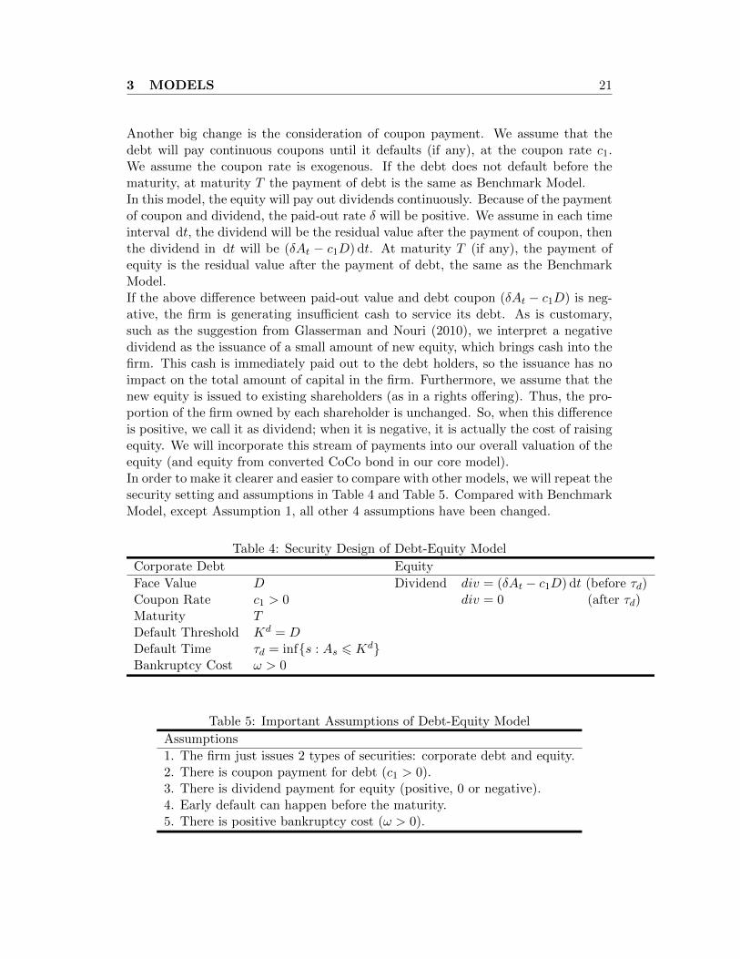
Another big change is the consideration of coupon payment. We assume that thedebt will pay continuous coupons until it defaults (if any), at the coupon rate c1.We assume the coupon rate is exogenous. If the debt does not default before thematurity, at maturity T the payment of debt is the same as Benchmark Model.In this model, the equity will pay out dividends continuously. Because of the paymentof coupon and dividend, the paid-out rate δ will be positive. We assume in each timeinterval dt, the dividend will be the residual value after the payment of coupon, thenthe dividend in dt will be (δAt − c1D) dt. At maturity T (if any), the payment ofequity is the residual value after the payment of debt, the same as the BenchmarkModel.If the above difference between paid-out value and debt coupon (δAt − c1D) is neg-ative, the firm is generating insufficient cash to service its debt. As is customary,such as the suggestion from Glasserman and Nouri (2010), we interpret a negativedividend as the issuance of a small amount of new equity, which brings cash into thefirm. This cash is immediately paid out to the debt holders, so the issuance has noimpact on the total amount of capital in the firm. Furthermore, we assume that thenew equity is issued to existing shareholders (as in a rights offering). Thus, the pro-portion of the firm owned by each shareholder is unchanged. So, when this differenceis positive, we call it as dividend; when it is negative, it is actually the cost of raisingequity. We will incorporate this stream of payments into our overall valuation of theequity (and equity from converted CoCo bond in our core model).In order to make it clearer and easier to compare with other models, we will repeat thesecurity setting and assumptions in Table 4 and Table 5. Compared with BenchmarkModel, except Assumption 1, all other 4 assumptions have been changed.

Table 4: Security Design of Debt-Equity Model

Corporate Debt Equity

Face Value D Dividend div = (δAt − c1D) dt (before τd)Coupon Rate c1 > 0 div = 0 (after τd)Maturity TDefault Threshold Kd = DDefault Time τd = infs : As 6 KdBankruptcy Cost ω > 0

Table 5: Important Assumptions of Debt-Equity Model

Assumptions

1. The firm just issues 2 types of securities: corporate debt and equity.2. There is coupon payment for debt (c1 > 0).3. There is dividend payment for equity (positive, 0 or negative).4. Early default can happen before the maturity.5. There is positive bankruptcy cost (ω > 0).

3 MODELS 22


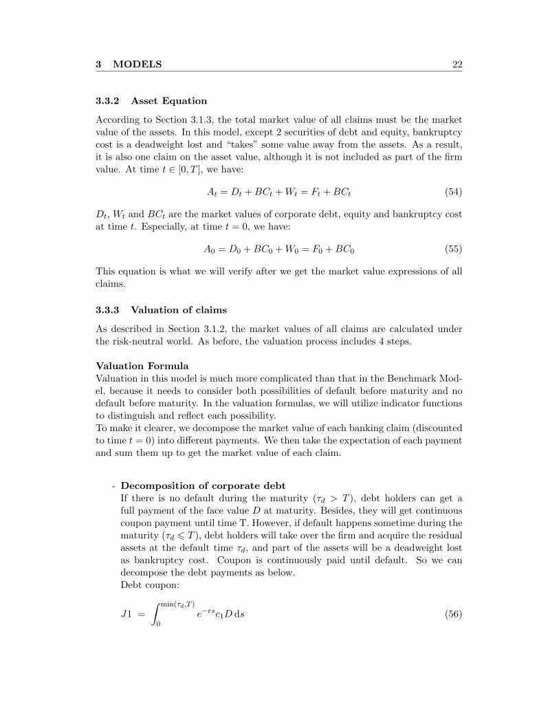
According to Section 3.1.3, the total market value of all claims must be the marketvalue of the assets. In this model, except 2 securities of debt and equity, bankruptcycost is a deadweight lost and “takes” some value away from the assets. As a result,it is also one claim on the asset value, although it is not included as part of the firmvalue. At time t ∈ [0, T ], we have:

At = Dt +BCt +Wt = Ft +BCt (54)

Dt, Wt and BCt are the market values of corporate debt, equity and bankruptcy costat time t. Especially, at time t = 0, we have:

A0 = D0 +BC0 +W0 = F0 +BC0 (55)

This equation is what we will verify after we get the market value expressions of allclaims.


As described in Section 3.1.2, the market values of all claims are calculated underthe risk-neutral world. As before, the valuation process includes 4 steps.

Valuation FormulaValuation in this model is much more complicated than that in the Benchmark Mod-el, because it needs to consider both possibilities of default before maturity and nodefault before maturity. In the valuation formulas, we will utilize indicator functionsto distinguish and reflect each possibility.To make it clearer, we decompose the market value of each banking claim (discountedto time t = 0) into different payments. We then take the expectation of each paymentand sum them up to get the market value of each claim.

- Decomposition of corporate debtIf there is no default during the maturity (τd > T ), debt holders can get afull payment of the face value D at maturity. Besides, they will get continuouscoupon payment until time T. However, if default happens sometime during thematurity (τd 6 T ), debt holders will take over the firm and acquire the residualassets at the default time τd, and part of the assets will be a deadweight lostas bankruptcy cost. Coupon is continuously paid until default. So we candecompose the debt payments as below.Debt coupon:

J1 =

∫ min(τd,T )

0e−rsc1D ds (56)

3 MODELS 23

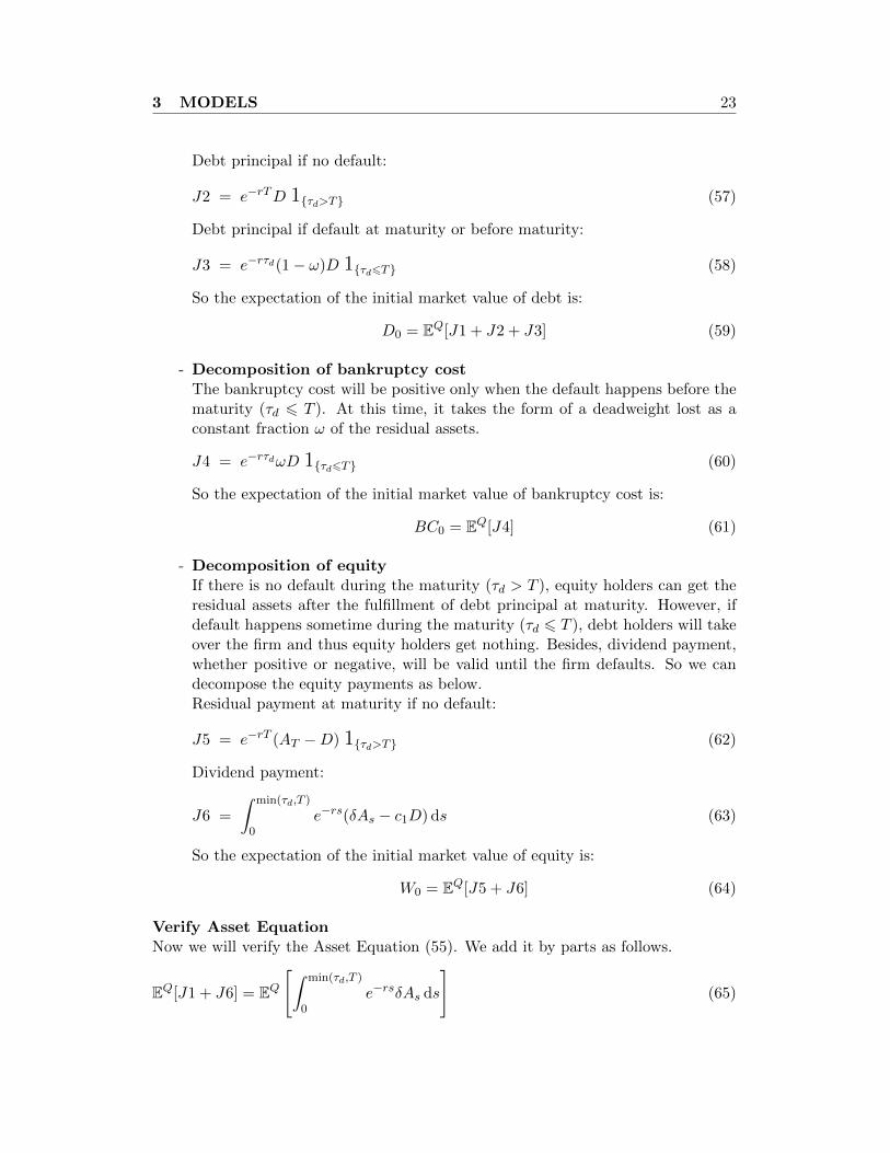
Debt principal if no default:

J2 = e−rTD 1τd>T (57)

Debt principal if default at maturity or before maturity:

J3 = e−rτd(1− ω)D 1τd6T (58)

So the expectation of the initial market value of debt is:

D0 = EQ[J1 + J2 + J3] (59)

- Decomposition of bankruptcy costThe bankruptcy cost will be positive only when the default happens before thematurity (τd 6 T ). At this time, it takes the form of a deadweight lost as aconstant fraction ω of the residual assets.

J4 = e−rτdωD 1τd6T (60)

So the expectation of the initial market value of bankruptcy cost is:

BC0 = EQ[J4] (61)

- Decomposition of equityIf there is no default during the maturity (τd > T ), equity holders can get theresidual assets after the fulfillment of debt principal at maturity. However, ifdefault happens sometime during the maturity (τd 6 T ), debt holders will takeover the firm and thus equity holders get nothing. Besides, dividend payment,whether positive or negative, will be valid until the firm defaults. So we candecompose the equity payments as below.Residual payment at maturity if no default:

J5 = e−rT (AT −D) 1τd>T (62)

Dividend payment:

J6 =

∫ min(τd,T )

0e−rs(δAs − c1D) ds (63)

So the expectation of the initial market value of equity is:

W0 = EQ[J5 + J6] (64)

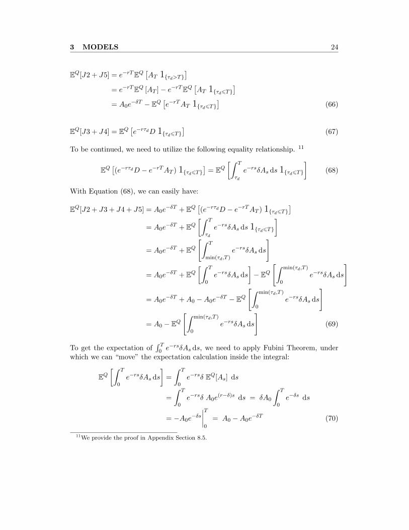
Verify Asset EquationNow we will verify the Asset Equation (55). We add it by parts as follows.

EQ[J1 + J6] = EQ[∫ min(τd,T )

0e−rsδAs ds

](65)

3 MODELS 24

EQ[J2 + J5] = e−rTEQ[AT 1τd>T

]= e−rTEQ [AT ]− e−rTEQ

[AT 1τd6T

]= A0e

−δT − EQ[e−rTAT 1τd6T

](66)

EQ[J3 + J4] = EQ[e−rτdD 1τd6T

](67)

To be continued, we need to utilize the following equality relationship. 11

EQ[(e−rτdD − e−rTAT ) 1τd6T

]= EQ

[∫ T

τd

e−rsδAs ds 1τd6T]

(68)

With Equation (68), we can easily have:

EQ[J2 + J3 + J4 + J5] = A0e−δT + EQ

[(e−rτdD − e−rTAT ) 1τd6T

]= A0e

−δT + EQ[∫ T

τd

e−rsδAs ds 1τd6T]

= A0e−δT + EQ

[∫ T

min(τd,T )e−rsδAs ds

]

= A0e−δT + EQ

[∫ T

0e−rsδAs ds

]− EQ

[∫ min(τd,T )

0e−rsδAs ds

]

= A0e−δT +A0 −A0e

−δT − EQ[∫ min(τd,T )

0e−rsδAs ds

]

= A0 − EQ[∫ min(τd,T )

0e−rsδAs ds

](69)

To get the expectation of∫ T0 e−rsδAs ds, we need to apply Fubini Theorem, under

which we can “move” the expectation calculation inside the integral:

EQ[∫ T

0e−rsδAs ds

]=

∫ T

0e−rsδ EQ[As] ds

=

∫ T

0e−rsδ A0e

(r−δ)s ds = δA0

∫ T

0e−δs ds

= −A0e−δs∣∣∣∣T0

= A0 −A0e−δT (70)

11We provide the proof in Appendix Section 8.5.

3 MODELS 25

Based on (65) and (69), we have:

D0 +BC0 +W0 = EQ[J1 + J2 + J3 + J4 + J5 + J6]

= EQ[(J1 + J6) + (J2 + J3 + J4 + J5)]

= EQ[∫ min(τd,T )

0e−rsδAs ds

]+A0 − EQ

[∫ min(τd,T )

0e−rsδAs ds

]= A0 (71)

Now we have verified Asset Equation (55).Note that the present market value of coupon and dividend payment (J1 + J6)is equal to the present value of total cash outflow during the maturity, which is∫ min(τd,T )0 e−rsδAs ds, rather than

∫ T0 e−rsδAs ds. Actually, the difference of these

two terms∫ Tmin(τd,T )

e−rsδAs ds is never produced by the firm because the firm willnot have any cash outflow after it defaults at τd. All the assets are taken over bydebt holders and the firm does not exist after default. But for calculation purpose,this term will appears in our mathematical derivation.

Explicit FormulaAfter some intensive mathematical derivation, we can get the risk-neutral expectationof each decomposition payment. 12 Since we use indicator function to reflect whetherdefault or not during the maturity, H function, containing indicator function as onemultiplier, will be used widely to achieve the explicit formula of the expectation.The definition, property and some basic calculation of functions H(·) are described

in Section 3.1.4. Remember that we have θ = −µσ +

√µ2

σ2 + 2r for all the calculationformulas in our paper.

EQ[J1] =c1D

r

1− e−rT[1−H

(T, 0, 0, log

Kd

A0

)]− e−rT

(Kd

A0

)− θσ

H

(T,θ

σ, 0, log

Kd

A0

)(72)

EQ[J2] = e−rTD

[1−H

(T, 0, 0, log

Kd

A0

)](73)

EQ[J3] = e−rT (1− ω)D

(Kd

A0

)− θσ

H

(T,θ

σ, 0, log

Kd

A0

)(74)

EQ[J4] = e−rTωD

(Kd

A0

)− θσ

H

(T,θ

σ, 0, log

Kd

A0

)(75)

12To save space, we just provide the final formulas in the Main Body of this paper. A detailedderivation is deferred to Appendix Section 8.6.

3 MODELS 26

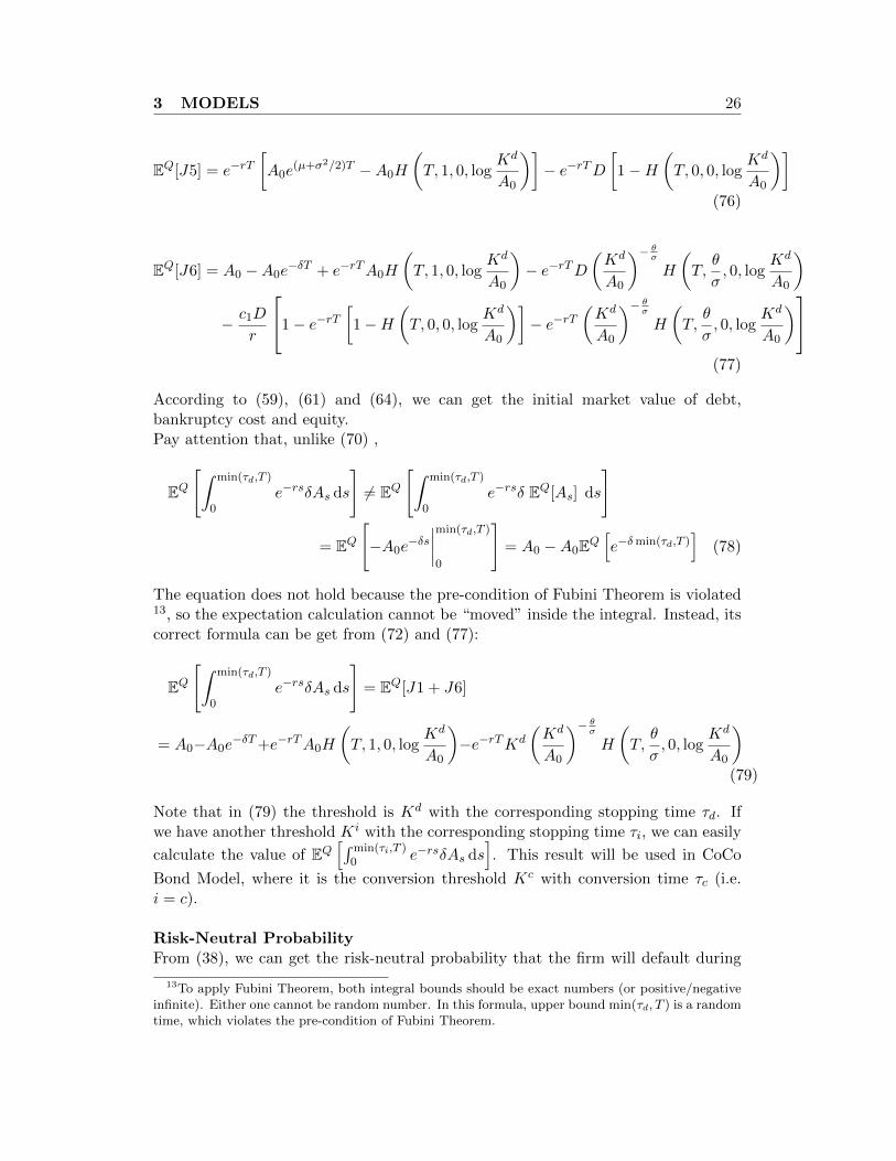
EQ[J5] = e−rT[A0e

(µ+σ2/2)T −A0H

(T, 1, 0, log

Kd

A0

)]− e−rTD

[1−H

(T, 0, 0, log

Kd

A0

)](76)

EQ[J6] = A0 −A0e−δT + e−rTA0H

(T, 1, 0, log

Kd

A0

)− e−rTD

(Kd

A0

)− θσ

H

(T,θ

σ, 0, log

Kd

A0

)

− c1D

r

1− e−rT[1−H

(T, 0, 0, log

Kd

A0

)]− e−rT

(Kd

A0

)− θσ

H

(T,θ

σ, 0, log

Kd

A0

)(77)

According to (59), (61) and (64), we can get the initial market value of debt,bankruptcy cost and equity.Pay attention that, unlike (70) ,

EQ[∫ min(τd,T )

0e−rsδAs ds

]6= EQ

[∫ min(τd,T )

0e−rsδ EQ[As] ds

]

= EQ[−A0e

−δs∣∣∣∣min(τd,T )

0

]= A0 −A0EQ

[e−δmin(τd,T )

](78)

The equation does not hold because the pre-condition of Fubini Theorem is violated13, so the expectation calculation cannot be “moved” inside the integral. Instead, itscorrect formula can be get from (72) and (77):

EQ[∫ min(τd,T )

0e−rsδAs ds

]= EQ[J1 + J6]

= A0−A0e−δT+e−rTA0H

(T, 1, 0, log

Kd

A0

)−e−rTKd

(Kd

A0

)− θσ

H

(T,θ

σ, 0, log

Kd

A0

)(79)

Note that in (79) the threshold is Kd with the corresponding stopping time τd. Ifwe have another threshold Ki with the corresponding stopping time τi, we can easily

calculate the value of EQ[∫ min(τi,T )

0 e−rsδAs ds]. This result will be used in CoCo

Bond Model, where it is the conversion threshold Kc with conversion time τc (i.e.i = c).

Risk-Neutral ProbabilityFrom (38), we can get the risk-neutral probability that the firm will default during

13To apply Fubini Theorem, both integral bounds should be exact numbers (or positive/negativeinfinite). Either one cannot be random number. In this formula, upper bound min(τd, T ) is a randomtime, which violates the pre-condition of Fubini Theorem.

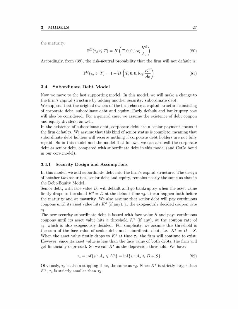
3 MODELS 27

the maturity.

PQ(τd 6 T ) = H

(T, 0, 0, log

Kd

A0

)(80)

Accordingly, from (39), the risk-neutral probability that the firm will not default is:

PQ(τd > T ) = 1−H(T, 0, 0, log

Kd

A0

)(81)

3.4 Subordinate Debt Model

Now we move to the last supporting model. In this model, we will make a change tothe firm’s capital structure by adding another security: subordinate debt.We suppose that the original owners of the firm choose a capital structure consistingof corporate debt, subordinate debt and equity. Early default and bankruptcy costwill also be considered. For a general case, we assume the existence of debt couponand equity dividend as well.In the existence of subordinate debt, corporate debt has a senior payment status ifthe firm defaults. We assume that this kind of senior status is complete, meaning thatsubordinate debt holders will receive nothing if corporate debt holders are not fullyrepaid. So in this model and the model that follows, we can also call the corporatedebt as senior debt, compared with subordinate debt in this model (and CoCo bondin our core model).


In this model, we add subordinate debt into the firm’s capital structure. The designof another two securities, senior debt and equity, remains nearly the same as that inthe Debt-Equity Model.Senior debt, with face value D, will default and go bankruptcy when the asset valuefirstly drops to threshold Kd = D at the default time τd. It can happen both beforethe maturity and at maturity. We also assume that senior debt will pay continuouscoupons until its asset value hits Kd (if any), at the exogenously decided coupon ratec1.The new security subordinate debt is issued with face value S and pays continuouscoupons until its asset value hits a threshold Ks (if any), at the coupon rate ofc2, which is also exogenously decided. For simplicity, we assume this threshold isthe sum of the face value of senior debt and subordinate debt, i.e. Ks = D + S.When the asset value firstly drops to Ks at time τs, the firm will continue to exist.However, since its asset value is less than the face value of both debts, the firm willget financially depressed. So we call Ks as the depression threshold. We have:

τs = infs : As 6 Ks = infs : As 6 D + S (82)

Obviously, τs is also a stopping time, the same as τd. Since Ks is strictly larger thanKd, τs is strictly smaller than τd.

3 MODELS 28

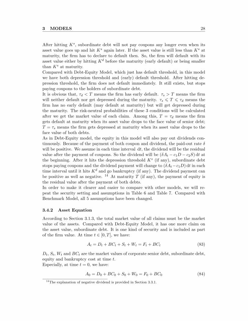
After hitting Ks, subordinate debt will not pay coupons any longer even when itsasset value goes up and hit Ks again later. If the asset value is still less than Ks atmaturity, the firm has to declare to default then. So, the firm will default with itsasset value either by hitting Kd before the maturity (early default) or being smallerthan Ks at maturity.Compared with Debt-Equity Model, which just has default threshold, in this modelwe have both depression threshold and (early) default threshold. After hitting de-pression threshold, the firm does not default immediately. It still exists, but stopspaying coupons to the holders of subordinate debt.It is obvious that, τd < T means the firm has early default. τs > T means the firmwill neither default nor get depressed during the maturity. τs 6 T 6 τd means thefirm has no early default (may default at maturity) but will get depressed duringthe maturity. The risk-neutral probabilities of these 3 conditions will be calculatedafter we get the market value of each claim. Among this, T = τd means the firmgets default at maturity when its asset value drops to the face value of senior debt;T = τs means the firm gets depressed at maturity when its asset value drops to theface value of both debts.As in Debt-Equity model, the equity in this model will also pay out dividends con-tinuously. Because of the payment of both coupon and dividend, the paid-out rate δwill be positive. We assume in each time interval dt, the dividend will be the residualvalue after the payment of coupons. So the dividend will be (δAt − c1D− c2S) dt atthe beginning. After it hits the depression threshold Ks (if any), subordinate debtstops paying coupons and the dividend payment will change to (δAt−c1D) dt in eachtime interval until it hits Kd and go bankruptcy (if any). The dividend payment canbe positive as well as negative. 14 At maturity T (if any), the payment of equity isthe residual value after the payment of both debts.In order to make it clearer and easier to compare with other models, we will re-peat the security setting and assumptions in Table 6 and Table 7. Compared withBenchmark Model, all 5 assumptions have been changed.


According to Section 3.1.3, the total market value of all claims must be the marketvalue of the assets. Compared with Debt-Equity Model, it has one more claim onthe asset value, subordinate debt. It is one kind of security and is included as partof the firm value. At time t ∈ [0, T ], we have:

At = Dt +BCt + St +Wt = Ft +BCt (83)

Dt, St, Wt and BCt are the market values of corporate senior debt, subordinate debt,equity and bankruptcy cost at time t.Especially, at time t = 0, we have:

A0 = D0 +BC0 + S0 +W0 = F0 +BC0 (84)

14The explanation of negative dividend is provided in Section 3.3.1.

3 MODELS 29

Table 6: Security Design of Subordinate Debt Model

Corporate Senior Debt Subordinate Debt

Face Value D Face Value SCoupon Rate c1 > 0 Coupon Rate c2 > 0Maturity T Maturity TDefault Threshold Kd = D Depression Threshold Ks = D + SDefault Time τd = infs : As 6 Kd Depression Time τs = infs : As 6 KsBankruptcy Cost ω > 0 Depression Cost ω′ = 0

Equity

Dividend div = (δAt − c1D − c2S) dt (before τs)div = (δAt − c1D) dt (after τs and before τd)div = 0 (after τd)

Table 7: Important Assumptions of Subordinate Debt Model

Assumptions

1. The firm issues 3 types of securities, including subordinate debt.2. There is coupon payment for both debts (c1 > 0, c2 > 0).3. There is dividend payment for equity (positive, 0 or negative).4. Early default can happen before the maturity.5. There is positive bankruptcy cost (ω > 0).



As before, the market values of all claims are calculated under the risk-neutral world.We conduct the valuation in 4 steps.

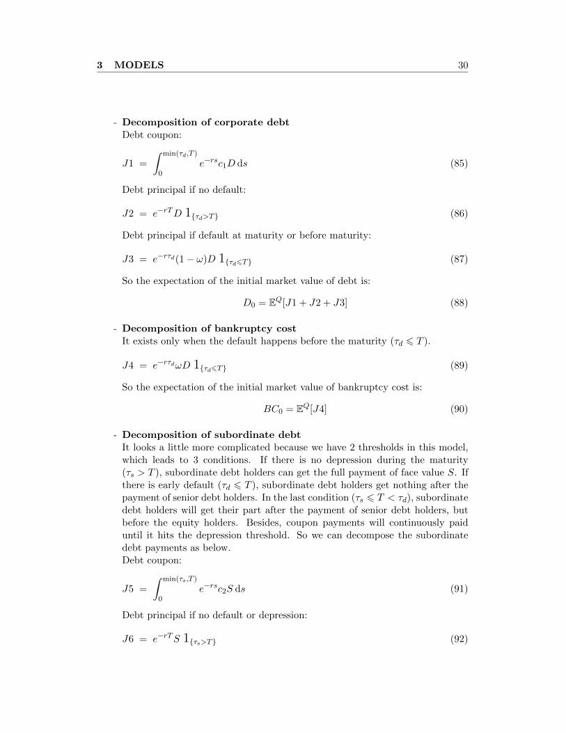
Valuation FormulaWe have 2 thresholds in this model, so there exist 3 different conditions. As before,we will utilize indicator functions to distinguish each possibility. We still decomposethe payments of each claim firstly, take the expectation of each payment and thensum them up to get the market value of each claim.The design of corporate debt is totally the same as that in Debt-Equity Model. Itsdynamics and threshold does not change after the introduction of subordinate debt.Its payment at any time in any condition (default or no default) keeps the sameas before. So in this model (also the CoCo Bond Model), the decomposition andvaluation of corporate debt payment is exactly the same as that in the Debt-EquityModel. Since the bankruptcy cost always comes with the corporate debt, its paymentalso keeps the same across the last 3 models. In order to make it complete, we stillrepeat their formulas here, without detailed explanation.

3 MODELS 30

- Decomposition of corporate debtDebt coupon:

J1 =

∫ min(τd,T )

0e−rsc1D ds (85)


J2 = e−rTD 1τd>T (86)


J3 = e−rτd(1− ω)D 1τd6T (87)


D0 = EQ[J1 + J2 + J3] (88)

- Decomposition of bankruptcy costIt exists only when the default happens before the maturity (τd 6 T ).



BC0 = EQ[J4] (90)

- Decomposition of subordinate debtIt looks a little more complicated because we have 2 thresholds in this model,which leads to 3 conditions. If there is no depression during the maturity(τs > T ), subordinate debt holders can get the full payment of face value S. Ifthere is early default (τd 6 T ), subordinate debt holders get nothing after thepayment of senior debt holders. In the last condition (τs 6 T < τd), subordinatedebt holders will get their part after the payment of senior debt holders, butbefore the equity holders. Besides, coupon payments will continuously paiduntil it hits the depression threshold. So we can decompose the subordinatedebt payments as below.Debt coupon:

J5 =

∫ min(τs,T )

0e−rsc2S ds (91)

Debt principal if no default or depression:

J6 = e−rTS 1τs>T (92)

3 MODELS 31

Debt principal if depression but no early default:

J7 = e−rT min(AT −D,S) 1τs6T<τd (93)

So the expectation of the initial market value of subordinate debt is:

S0 = EQ[J5 + J6 + J7] (94)

- Decomposition of equityThere are also 3 conditions. Equity holders will always be repaid after thepayment of both kinds of debt holders. Besides, dividend payment will be validuntil the firm defaults, and it will have a big change if the firm gets depressedbecause since then subordinate debt coupon is not paid.Residual payment at maturity if no default or depression:

J8 = e−rT (AT −D − S) 1τs>T (95)

Residual payment at maturity if depression but no early default:

J9 = e−rT max(AT −D − S, 0) 1τs6T<τd (96)

Dividend payment is the sum of the following 3 different conditions:

J10.1 =

∫ T

0e−rs(δAs − c1D − c2S) ds1τs>T (97)

J10.2 =

[∫ τs

0e−rs(δAs − c1D − c2S) ds+

∫ T

τs

e−rs(δAs − c1D) ds

]1τs6T<τd

(98)

J10.3 =

[∫ τs


∫ τd

τs


]1τd6T

(99)

J10 = J10.1 + J10.2 + J10.3

=

∫ min(τs,T )


∫ min(τd,T )

τs

e−rs(δAs − c1D) ds1τs6T(100)


W0 = EQ[J8 + J9 + J10] (101)

3 MODELS 32

Verify Asset EquationNow we will verify the Asset Equation (84). We add it by parts as follows.

EQ[J1 + J5 + J10]


0e−rsc1D ds+

∫ min(τs,T )

0e−rsc2S ds

+

∫ min(τs,T )


∫ min(τd,T )

τs

e−rs(δAs − c1D) ds1τs6T

]


0e−rsc1D ds+

∫ min(τs,T )

0e−rs(δAs − c1D) ds+

∫ min(τd,T )

τs


]


0e−rsc1D ds+

∫ τs

0e−rs(δAs − c1D) ds1τs6T

+

∫ T

0e−rs(δAs − c1D) ds1τs>T +

∫ min(τd,T )

τs


]


0e−rsc1D ds+

∫ min(τd,T )

0e−rs(δAs − c1D) ds1τs6T +

∫ T

0e−rs(δAs − c1D) ds1τs>T

]


0e−rsc1D ds+

∫ min(τd,T )

0e−rs(δAs − c1D) ds

]


0e−rsδAs ds

](102)

Above, if τs > T , then T < τd. So we have T = min(T, τd) when τs > T .


](103)

EQ[J6 + J8] = EQ[e−rT (AT −D) 1τs>T

](104)

EQ[J7 + J9] = EQ[e−rT (AT −D) 1τs6T<τd

](105)

EQ[(J6 + J8) + (J7 + J9) + J2]

= EQ[e−rT (AT −D) 1τs>T + e−rT (AT −D) 1τs6T<τd + e−rTD 1τd>T

]= EQ

[e−rT (AT −D) 1τd>T + e−rTD 1τd>T

]= EQ

[e−rTAT 1τd>T

](106)

3 MODELS 33

The result of (102), (103) and (106) is exactly the same as (65), (67) and (66),accordingly.As (69) and (71), based on (102), (103) and (106), we can calculate that:

D0 +BC0 + S0 +W0

= EQ[J1 + J2 + J3 + J4 + J5 + J6 + J7 + J8 + J9 + J10

]= EQ

[(J1 + J5 + J10) + [(J2 + J6 + J7 + J8 + J9) + (J3 + J4)]

]= EQ

[∫ min(τd,T )

0e−rsδAs ds

]+A0 − EQ

[∫ min(τd,T )

0e−rsδAs ds

]= A0 (107)

Now we have verified Asset Equation (84).Note that the present market value of coupons and dividend payment (J1+J5+J10)is equal to the present value of total cash outflow during the maturity, which is∫ min(τd,T )0 e−rsδAs ds.

Explicit FormulaWe can get the explicit formula of the risk neutral expectation of each decompositionpayment with some forms of H function and ∆Hs function (∆H i function in Section3.1.4 by letting i = s). 15

EQ[J1] =c1D

r

1− e−rT[1−H

(T, 0, 0, log

Kd

A0

)]− e−rT

(Kd

A0

)− θσ

H

(T,θ

σ, 0, log

Kd

A0

)(108)

EQ[J2] = e−rTD

[1−H

(T, 0, 0, log

Kd

A0

)](109)

EQ[J3] = e−rT (1− ω)D

(Kd

A0

)− θσ

H

(T,θ

σ, 0, log

Kd

A0

)(110)

EQ[J4] = e−rTωD

(Kd

A0

)− θσ

H

(T,θ

σ, 0, log

Kd

A0

)(111)

EQ[J5] =c2S

r

[1− e−rT

[1−H

(T, 0, 0, log

Ks

A0

)]− e−rT

(Ks

A0

)− θσ

H

(T,θ

σ, 0, log

Ks

A0

)](112)

15A detailed derivation for the explicit formulas is deferred to Appendix Section 8.8.

3 MODELS 34

EQ[J6] = e−rTS

[1−H

(T, 0, 0, log

Ks

A0

)](113)

EQ[J7] = e−rT [A0∆Hs(T, 1, 0)−D∆Hs(T, 0, 0)]− EQ[J9] (114)

EQ[J8] = e−rT[A0e

(µ+σ2/2)T −A0H

(T, 1, 0, log

Ks

A0

)]− e−rT (D + S)

[1−H

(T, 0, 0, log

Ks

A0

)](115)

In order to solve EQ[J9], we can make the following transformation.

EQ[J9] = e−rTEQ[max(AT −D − S, 0) 1τs 6 T < τd

]= e−rTEQ

max(AT −D − S, 0) 1Kd < min06t6T

At 6 Ks

= e−rTEQ

max(AT −D − S, 0) 1 min06t6T

At 6 Ks −max(AT −D − S, 0) 1 min06t6T

At 6 Kd

(116)

We can solve the expectation value of J9 by regarding it as the difference of 2 barrieroptions, more specifically, 2 down-and-in call barrier options (CBdin).The down-and-in call barrier option has the following definition and valuation formu-la. If the underlying stock price (or asset value) with initial value S0 meets the GBMprocess with drift r and diffusion σ under Q-measure. If it goes down and reachesthe barrier H, the option becomes a vanilla European call option with strike price Kand maturity T . If the stock price does not reach the barrier H during the maturityT , the option expires worthless. 16

If the barrier H is not larger than the strike K (H 6 K), its initial price is:

CBdin(S0,K,H) = S0

(H

S0

)( 2rσ2

+1)

Φ(d3)− e−rTK(H

S0

)( 2rσ2−1)

Φ(d4) (117)

As before, Φ(·) is the CDF of standard normal distribution, and

d3 =log(H2

S0K

)+ (r + σ2/2)T

σ√T

(118)

d4 =log(H2

S0K

)+ (r − σ2/2)T

σ√T

= d3 − σ√T (119)

16A detailed derivation of the following pricing formula is provided in Appendix Section 8.7.

3 MODELS 35

Note that, since the drift (under Q-measure) in our model is r−δ, we need to replacer in (117), (118) and (119) as r − δ. Other parameters, σ and T , can be applieddirectly.We can treat the expectation of J9 as the difference of 2 barrier options, both withthe underlying asset value At and strike (D + S). The first one has a barrier of Ks,which is equal to the strike, and the second one has a barrier of Kd, which is smallerthan the strike. So we have:

EQ[J9] = CBdin(A0, D + S,Ks)− CBdin(A0, D + S,Kd) (120)

After getting the result of EQ[J9], the result of EQ[J7] can easily be got from (114).After getting the expectation from J1 to J9, the expectation of J10 (EQ[J10]) canbe easily got by deducting all the 9 other terms from A0. Since its formula is verylong, we will not show it here but defer it to Appendix.According to (88), (90), (94) and (101), we can get the initial market value of seniordebt, bankruptcy cost, subordinate debt and equity.

Risk-Neutral ProbabilityAs the previous models, we can also get the risk-neutral probability of each condition.Since we have 2 thresholds in this model, we have 3 risk-neutral probabilities for 3different conditions.The risk-neutral probability that the firm will early default before the maturity is:

PQ(τd < T ) = H

(T, 0, 0, log

Kd

A0

)(121)

The risk-neutral probability that the firm will neither default nor get depressed duringthe maturity is:

PQ(τs > T ) = 1−H(T, 0, 0, log

Ks

A0

)(122)

The risk-neutral probability that the firm has no early default(may get default atmaturity) but will get depressed during the maturity is:

PQ(τs 6 T 6 τd) = ∆Hs (T, 0, 0) (123)

Note that, (121) is the risk-neutral probability of early default. Since the firm canalso get default if its asset value is smaller than Ks at maturity, the risk-neutralprobability of default will be bigger after taking the late default into consideration.This probability will be calculated in Section 4.1.1.

3.5 CoCo Bond Model

Now it comes to our most important and core model. Instead of subordinate debt,we will add CoCo bond as the third security into the firm’s capital structure. Itsconversion mechanism and important role in the enhancement of financial stabilityis described in Section 1 and Section 2.

3 MODELS 36

We suppose that the original owners of the firm choose a capital structure consistingof corporate debt, CoCo bond and equity. Early default and bankruptcy cost willalso be considered. For a general case, we will assume the existence of debt couponand equity dividend as well.


In this model, we add CoCo bond into the firm’s capital structure. The design ofanother two securities, senior debt and equity, remains nearly the same as that in theDebt-Equity Model and Subordinate Debt Model.Senior debt, with face value D, will default and go bankruptcy when the asset valuedrops to threshold Kd = D at the default time τd. It can happen both before thematurity and at maturity. We also assume that senior debt will pay continuouscoupons until its asset value hits Kd (if any), at the coupon rate of c1, which isdecided exogenously.The new security CoCo bond is issued as debt in the capital structure with facevalue C, and it will keep as debt and pay continuous coupons at exogenously decidedcoupon rate c3 until the asset value firstly drops to a threshold Kc at time τc (if any).We call Kc as conversion threshold and at this time CoCo bond will automaticallyconvert into equity to supplement the firm’s capital position. After conversion, CoCobond does not exist anymore and the CoCo bond holders will receive a pre-specifiedfraction α of the remaining equity. α is called the conversion ratio and has the rangeof 0 < α < 1.We define Kc and τc as:

Kc = (1 + β)(D + C) (124)

τc = infs : As 6 Kc = infs : As 6 (1 + β)(D + C) (125)

Obviously τc is also a stopping time. β is the threshold parameter and decides thedistance of conversion threshold from the face value of senior debt and CoCo bond.We set its range as 0 < β < 1. The relationship between two thresholds and two facevalues in this model is:

Kd = D < D + C < Kc (126)

Since Kc is strictly larger than Kd, τc is strictly smaller than τd.It is obvious that, τd 6 T means the firm will go bankruptcy during the maturity, andits CoCo bond has been converted before the bankruptcy. τc > T means the firm willneither convert its CoCo bond nor default during the maturity. τc 6 T < τd meansthe firm’s CoCo bond will convert into equity but the firm will not go bankruptcyduring the maturity. The risk-neutral probabilities of these 3 conditions will becalculated after we get the market value of each claim. Among this, T = τd meansthe firm gets default at maturity when its asset value drops below the face value ofsenior debt; T = τs means the firm converts into CoCo bond at maturity when itsasset value hits Kc.As in Debt-Equity Model and Subordinate Debt Model, the equity in this model willalso pay out dividends continuously. Because of the payment of both coupons and

3 MODELS 37

dividend, the paid-out rate δ will be positive. We assume in each time interval dt,the dividend will be the residual value after the payment of any possible coupons.So the dividend will be (δAt − c1D − c3C) dt at the beginning. After it hits theconversion threshold Kc, CoCo bond converts into equity and stops paying coupons,so the dividend payment will change to (δAt− c1D) dt in each time interval, before ithits Kd and go bankruptcy (if any). The dividend payment can be positive as well asnegative. At maturity T (if any), the payment of equity is the residual value after thepayment of debt, the same as that in Debt-Equity Model. If conversion happens, theoriginal CoCo bond holder, i.e. the new equity holder will receive a fraction α of thedividend during the maturity and a fraction α of the residual payment at maturity(if any).In order to make it clearer and easier to compare with other models, we will repeat thesecurity setting and assumptions in Table 8 and Table 9. Compared with BenchmarkModel, all 5 assumptions have been changed.

Table 8: Security Design of CoCo Bond Model

Corporate Senior Debt CoCo Bond

Face Value D Face Value CCoupon Rate c1 > 0 Coupon Rate c3 > 0Maturity T Maturity TDefault Threshold Kd = D Conversion Threshold Kc = (1 + β)(D + C)Default Time τd = infs : As 6 Kd Conversion Time τc = infs : As 6 KcBankruptcy Cost ω > 0 Conversion Ratio 0 < α < 1

Equity

Dividend div = (δAt − c1D − c3C) dt (before τc)div = (δAt − c1D) dt (after τc and before τd)div = 0 (after τd)

Table 9: Important Assumptions of CoCo Bond Model

Assumptions

1. The firm issues 3 types of securities, including CoCo Bond.2. There is coupon payment for both debts (c1 > 0, c3 > 0).3. There is dividend payment for equity (positive, 0 or negative).4. Early default can happen before the maturity.5. There is positive bankruptcy cost (ω > 0).


According to Section 3.1.3, the total market value of all claims must be the marketvalue of the assets. Compared with Subordinate Debt Model, it has another claimon the asset value, CoCo bond. It is also one kind of security and is included as part

3 MODELS 38

of the firm value as well. At time t ∈ [0, T ], we have:

At = Dt +BCt + CCBt +Wt = Ft +BCt (127)

Dt, CCBt, Wt and BCt are the market values of corporate senior debt, CoCo bond,equity and bankruptcy cost at time t. Especially, at time t = 0, we have:

A0 = D0 +BC0 + CCB0 +W0 = F0 +BC0 (128)



As described before, the market values of all claims are calculated under the risk-neutral world. Valuation is conducted in 4 steps.

Valuation FormulaAs before, we will utilize indicator functions to distinguish 3 possibilities in this mod-el. We still decompose the payments of each claim firstly, take the expectation of eachpayment and then sum them up to get the market value of each claim. As describedin Section 3.4.3, the decomposition of corporate debt payment and bankruptcy costis exactly the same as that in the Debt-Equity Model and Subordinate Debt Model.In order to make it complete, we still repeat their formulas here.

- Decomposition of corporate debtDebt coupon:

J1 =

∫ min(τd,T )

0e−rsc1D ds (129)


J2 = e−rTD 1τd>T (130)


J3 = e−rτd(1− ω)D 1τd6T (131)


D0 = EQ[J1 + J2 + J3] (132)

- Decomposition of bankruptcy costIt exists only when the default happens before the maturity (τd 6 T ).



BC0 = EQ[J4] (134)

3 MODELS 39

- Decomposition of CoCo bondWe have both conversion trigger and default trigger, so there exist 3 conditions.If there is no conversion during the maturity (τc > T ), CoCo bond holderscan get the full payment of face value C at maturity. There is also couponpayment before conversion. Otherwise CoCo bond will convert into equity andthe original CoCo bond holders will share a fraction α of the remaining equity.If there is early default after conversion (τd 6 T ), original CoCo bond holders,i.e. new equity holders, will only get the dividend payment. If there is no earlydefault after conversion (τc 6 T < τd), they can have a final payment as well asdividend payment. So we can decompose the CoCo bond payments as below.Debt coupon:

J5 =

∫ min(τc,T )

0e−rsc3C ds (135)

CCB principal if no conversion:

J6 = e−rTC 1τc>T (136)

Share of equity value if conversion at maturity or before maturity:

J7 = e−rTα(AT −D) 1τc6T<τd (137)

Share of dividend payment if conversion at maturity or before maturity:

J8 = α

∫ min(τd,T )

τc

e−rs(δAs − c1D) ds 1τc6T (138)

So the expectation of the initial market value of CoCo bond is:

CCB0 = EQ[J5 + J6 + J7 + J8] (139)

- Decomposition of equityIf there is no conversion during the maturity (τc > T ), original equity holderscan get a final payment at maturity after the face value of both debts, aswell as dividend until maturity. Otherwise CoCo bond will convert into equityand the original equity holders will share a fraction (1 − α) of the remainingequity payment. Except for different fractions they get, the remaining equitypayment style will be the same for original equity holders and original CoCobond holders.Residual payment at maturity if no conversion:

J9 = e−rT (AT −D − C) 1τc>T (140)

Share of equity value if conversion at maturity or before maturity:

J10 = e−rT (1− α)(AT −D) 1τc6T<τd (141)

3 MODELS 40

Dividend payment is the sum of the following 3 different conditions:

J11.1 =

∫ T

0e−rs(δAs − c1D − c3C) ds1τc>T (142)

J11.2 =

[∫ τc

0e−rs(δAs − c1D − c3C) ds+ (1− α)

∫ T

τc


]1τc6T<τd

(143)

J11.3 =

[∫ τc

0e−rs(δAs − c1D − c3C) ds+ (1− α)

∫ τd

τc


]1τd6T

(144)

J11 = J11.1 + J11.2 + J11.3 (145)


W0 = EQ[J9 + J10 + J11] (146)

Verify Asset EquationWe will verify the Asset Equation (128). We add it by parts as follows.Similar to (100), we have:

J8 + J11 =

∫ min(τc,T )

0e−rs(δAs − c1D − c3C) ds+

∫ min(τd,T )

τc

e−rs(δAs − c1D) ds1τc6T

(147)

Similar to (102), we have:

EQ[J1 + J5 + J8 + J11] = EQ[∫ min(τd,T )

0e−rsδAs ds

](148)

Similar to (103)-(106), we have (149)-(152) as below:


](149)

EQ[J6 + J9] = EQ[e−rT (AT −D) 1τc>T

](150)

EQ[J7 + J10] = EQ[e−rT (AT −D) 1τc6T<τd

](151)

3 MODELS 41

EQ[(J6 + J9) + (J7 + J10) + J2]

= EQ[e−rT (AT −D) 1τc>T + e−rT (AT −D) 1τc6T<τd + e−rTD 1τd>T

]= EQ

[e−rT (AT −D) 1τd>T + e−rTD 1τd>T

]= EQ

[e−rTAT 1τd>T

](152)

As (107), we can calculate that:

D0 +BC0 + CCB0 +W0

= EQ[J1 + J2 + J3 + J4 + J5 + J6 + J7 + J9 + J10 + J8 + J11]


0e−rsδAs ds

]+A0 − EQ

[∫ min(τd,T )

0e−rsδAs ds

]= A0 (153)

Now we have verified Asset Equation (128).Note that the present market value of coupons and dividend payment (J1 + J5 +J8 + J11) is equal to the present value of total cash outflow during the maturity,

which is∫ min(τd,T )0 e−rsδAs ds.

Explicit FormulaWe can get the explicit formula of the risk neutral expectation of each decompositionpayment with some forms of H function and ∆Hc function (∆H i function in Section3.1.4 by letting i = c). 17.

EQ[J1] =c1D

r

1− e−rT[1−H

(T, 0, 0, log

Kd

A0

)]− e−rT

(Kd

A0

)− θσ

H

(T,θ

σ, 0, log

Kd

A0

)(154)

EQ[J2] = e−rTD

[1−H

(T, 0, 0, log

Kd

A0

)](155)

EQ[J3] = e−rT (1− ω)D

(Kd

A0

)− θσ

H

(T,θ

σ, 0, log

Kd

A0

)(156)

EQ[J4] = e−rTωD

(Kd

A0

)− θσ

H

(T,θ

σ, 0, log

Kd

A0

)(157)

17A detailed derivation for the explicit formulas is deferred to Appendix Section 8.9.

3 MODELS 42

EQ[J5] =c3C

r

[1− e−rT

[1−H

(T, 0, 0, log

Kc

A0

)]− e−rT

(Kc

A0

)− θσ

H

(T,θ

σ, 0, log

Kc

A0

)](158)

EQ[J6] = e−rTC

[1−H

(T, 0, 0, log

Kc

A0

)](159)

EQ[J7] = e−rTα [A0∆Hc(T, 1, 0)−D∆Hc(T, 0, 0)] (160)

EQ[J9] = e−rT[A0e

(µ+σ2/2)T −A0H

(T, 1, 0, log

Kc

A0

)]− e−rT (D + C)

[1−H

(T, 0, 0, log

Kc

A0

)](161)

EQ[J10] = e−rT (1− α) [A0∆Hc(T, 1, 0)−D∆Hc(T, 0, 0)] (162)

In order to get the expectation of J8, we can do the following transformation:

EQ[J8] = αEQ[∫ min(τd,T )

τc

e−rs(δAs − c1D) ds1τc6T

]

= αEQ[∫ min(τd,T )

min(τc,T )e−rs(δAs − c1D) ds

]


0e−rs(δAs − c1D) ds−

∫ min(τc,T )

0e−rs(δAs − c1D) ds

]


0e−rsδAs ds− J1−

∫ min(τc,T )

0e−rsδAs ds+

∫ min(τc,T )

0e−rsc1D ds

](163)

Among this, EQ[∫ min(τd,T )

0 e−rsδAs ds]

can be got as (79). EQ[∫ min(τc,T )

0 e−rsδAs ds]

just needs some changes of threshold from Kd (with stopping time τd) to Kc (with

stopping time τc), based on (79). EQ[∫ min(τc,T )

0 e−rsc1D ds]

just needs some change

of J5 from c3C to c1D, based on (158).After getting the expectation of J8, the expectation of J11 (EQ[J11]) can be easilygot by deducting all the 10 other terms from A0. Since the formula will be very long,we will not show it here but defer it to Appendix.According to (132), (134), (139) and (146), we can get the initial market value ofsenior debt, bankruptcy cost, CoCo bond and equity.

Risk-Neutral ProbabilityAs Subordinate Debt Model, we can also get the risk-neutral probability of 3 condi-tions.

4 CALIBRATION 43

The risk-neutral probability that the firm will default during the maturity:

PQ(τd 6 T ) = H

(T, 0, 0, log

Kd

A0

)(164)

The risk-neutral probability that the firm neither converses nor defaults:

PQ(τc > T ) = 1−H(T, 0, 0, log

Kc

A0

)(165)

The risk-neutral probability that the firm will convert its CoCo bond but will notdefault is:

PQ(τc 6 T < τd) = ∆Hc (T, 0, 0) (166)

4 Calibration

From the introduction of CoCo bond in Section 1 and Section 2, we have a qualitativeunderstanding of its contribution to the financial stability of the issuing firm as wellas the overall financial market. From the model part in Section 3, we can make aquantitative valuation for this security from our model construction. In the followingsection, we will further analyze quantitatively why it can be a good derivative securityby comparing with all other capital structures, based on all 4 models we developedin Section 3. More specifically, we will interpret its contribution from 2 perspectives:reducing the firm’s default probability, and mitigating the executive’s risk shiftingmotivation.

4.1 Default Probability

Policymakers and regulators are interested in monitoring the default probability ofa financial institution due to the potentially harmful effect of default on the realeconomy. For this reason, default probability of different models with different capitalstructures will be calculated and compared. Since the Benchmark Model is just anidealized simple start and it does not take early default into consideration, a veryimportant character of all other 3 models to decide the default probability, we willnot compare the default probability of this model below.For comparison purpose, we will calibrate the model with assumed parameter values.In order to compare different default probabilities of different capital structures, wehave to set other related parameters the same value for all 3 models, including thesame risk free interest rate r, value paid-out rate δ, volatility σ and maturity T .For capital structure parameter, we assume the initial asset value A0 and the totalface value of debts are the same across all 3 models, i.e. the same debt-equity ratioacross 3 models. In Debt-Equity Model, debt just takes the form of corporate debt.We assume its face value is D1. In Subordinate Debt Model, debt takes the form ofcorporate senior debt and subordinate debt. We assume their face values are D2 andS. In CoCo Bond Model, debt takes the form of corporate senior debt and CoCo

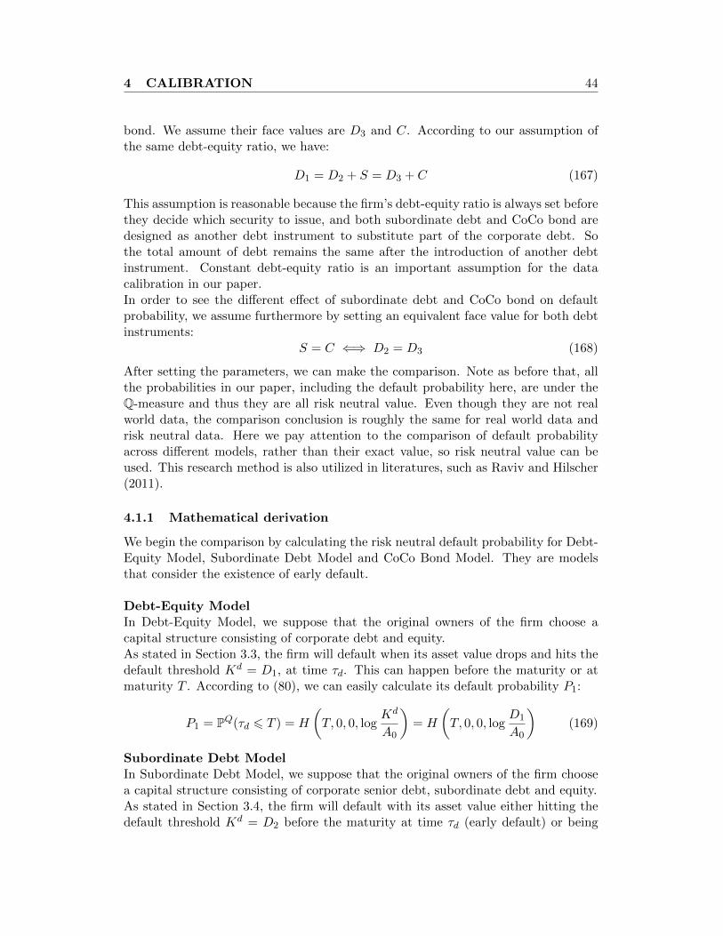
4 CALIBRATION 44

bond. We assume their face values are D3 and C. According to our assumption ofthe same debt-equity ratio, we have:

D1 = D2 + S = D3 + C (167)

This assumption is reasonable because the firm’s debt-equity ratio is always set beforethey decide which security to issue, and both subordinate debt and CoCo bond aredesigned as another debt instrument to substitute part of the corporate debt. Sothe total amount of debt remains the same after the introduction of another debtinstrument. Constant debt-equity ratio is an important assumption for the datacalibration in our paper.In order to see the different effect of subordinate debt and CoCo bond on defaultprobability, we assume furthermore by setting an equivalent face value for both debtinstruments:

S = C ⇐⇒ D2 = D3 (168)

After setting the parameters, we can make the comparison. Note as before that, allthe probabilities in our paper, including the default probability here, are under theQ-measure and thus they are all risk neutral value. Even though they are not realworld data, the comparison conclusion is roughly the same for real world data andrisk neutral data. Here we pay attention to the comparison of default probabilityacross different models, rather than their exact value, so risk neutral value can beused. This research method is also utilized in literatures, such as Raviv and Hilscher(2011).

4.1.1 Mathematical derivation

We begin the comparison by calculating the risk neutral default probability for Debt-Equity Model, Subordinate Debt Model and CoCo Bond Model. They are modelsthat consider the existence of early default.

Debt-Equity ModelIn Debt-Equity Model, we suppose that the original owners of the firm choose acapital structure consisting of corporate debt and equity.As stated in Section 3.3, the firm will default when its asset value drops and hits thedefault threshold Kd = D1, at time τd. This can happen before the maturity or atmaturity T . According to (80), we can easily calculate its default probability P1:

P1 = PQ(τd 6 T ) = H

(T, 0, 0, log

Kd

A0

)= H

(T, 0, 0, log

D1

A0

)(169)

Subordinate Debt ModelIn Subordinate Debt Model, we suppose that the original owners of the firm choosea capital structure consisting of corporate senior debt, subordinate debt and equity.As stated in Section 3.4, the firm will default with its asset value either hitting thedefault threshold Kd = D2 before the maturity at time τd (early default) or being

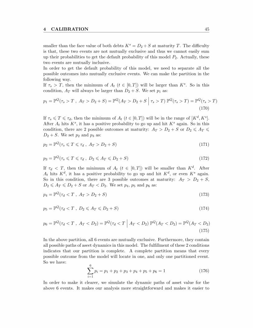
4 CALIBRATION 45

smaller than the face value of both debts Ks = D2 +S at maturity T . The difficultyis that, these two events are not mutually exclusive and thus we cannot easily sumup their probabilities to get the default probability of this model P2. Actually, thesetwo events are mutually inclusive.In order to get the default probability of this model, we need to separate all thepossible outcomes into mutually exclusive events. We can make the partition in thefollowing way.If τs > T , then the minimum of At (t ∈ [0, T ]) will be larger than Ks. So in thiscondition, AT will always be larger than D2 + S. We set p1 as:

p1 = PQ(τs > T , AT > D2 + S) = PQ(AT > D2 + S∣∣∣ τs > T ) PQ(τs > T ) = PQ(τs > T )

(170)

If τs 6 T 6 τd, then the minimum of At (t ∈ [0, T ]) will be in the range of [Kd,Ks].After At hits Ks, it has a positive probability to go up and hit Ks again. So in thiscondition, there are 2 possible outcomes at maturity: AT > D2 + S or D2 6 AT 6D2 + S. We set p2 and p3 as:

p2 = PQ(τs 6 T 6 τd , AT > D2 + S) (171)

p3 = PQ(τs 6 T 6 τd , D2 6 AT 6 D2 + S) (172)

If τd < T , then the minimum of At (t ∈ [0, T ]) will be smaller than Kd. AfterAt hits Kd, it has a positive probability to go up and hit Kd, or even Ks again.So in this condition, there are 3 possible outcomes at maturity: AT > D2 + S,D2 6 AT 6 D2 + S or AT < D2. We set p4, p5 and p6 as:

p4 = PQ(τd < T , AT > D2 + S) (173)

p5 = PQ(τd < T , D2 6 AT 6 D2 + S) (174)

p6 = PQ(τd < T , AT < D2) = PQ(τd < T∣∣∣ AT < D2) PQ(AT < D2) = PQ(AT < D2)

(175)

In the above partition, all 6 events are mutually exclusive. Furthermore, they containall possible paths of aseet dynamics in this model. The fulfillment of these 2 conditionsindicates that our partition is complete. A complete partition means that everypossible outcome from the model will locate in one, and only one partitioned event.So we have:

6∑i=1

pi = p1 + p2 + p3 + p4 + p5 + p6 = 1 (176)

In order to make it clearer, we simulate the dynamic paths of asset value for theabove 6 events. It makes our analysis more straightforward and makes it easier to

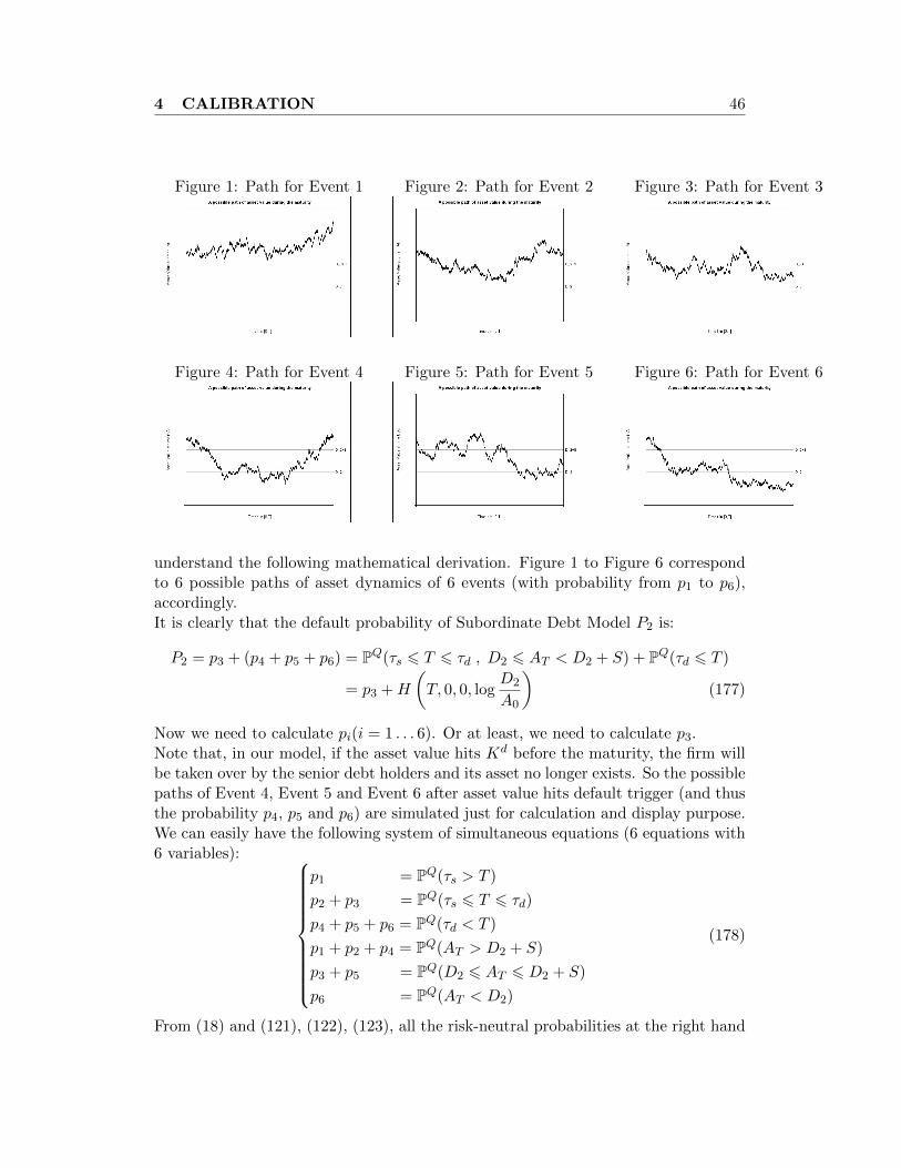
4 CALIBRATION 46

Figure 1: Path for Event 1 Figure 2: Path for Event 2 Figure 3: Path for Event 3

Figure 4: Path for Event 4 Figure 5: Path for Event 5 Figure 6: Path for Event 6

understand the following mathematical derivation. Figure 1 to Figure 6 correspondto 6 possible paths of asset dynamics of 6 events (with probability from p1 to p6),accordingly.It is clearly that the default probability of Subordinate Debt Model P2 is:

P2 = p3 + (p4 + p5 + p6) = PQ(τs 6 T 6 τd , D2 6 AT < D2 + S) + PQ(τd 6 T )

= p3 +H

(T, 0, 0, log

D2

A0

)(177)

Now we need to calculate pi(i = 1 . . . 6). Or at least, we need to calculate p3.Note that, in our model, if the asset value hits Kd before the maturity, the firm willbe taken over by the senior debt holders and its asset no longer exists. So the possiblepaths of Event 4, Event 5 and Event 6 after asset value hits default trigger (and thusthe probability p4, p5 and p6) are simulated just for calculation and display purpose.We can easily have the following system of simultaneous equations (6 equations with6 variables):

p1 = PQ(τs > T )

p2 + p3 = PQ(τs 6 T 6 τd)

p4 + p5 + p6 = PQ(τd < T )

p1 + p2 + p4 = PQ(AT > D2 + S)

p3 + p5 = PQ(D2 6 AT 6 D2 + S)

p6 = PQ(AT < D2)

(178)

From (18) and (121), (122), (123), all the risk-neutral probabilities at the right hand

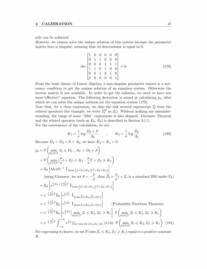
4 CALIBRATION 47

side can be achieved.However, we cannot solve the unique solution of this system because the parametermatrix here is singular, meaning that its determinant is equal to 0.

det

1 0 0 0 0 00 1 1 0 0 00 0 0 1 1 11 1 0 1 0 00 0 1 0 1 00 0 0 0 0 1

= 0 (179)

From the basic theory of Linear Algebra, a non-singular parameter matrix is a nec-essary condition to get the unique solution of an equation system. Otherwise theinverse matrix is not available. In order to get the solution, we need to have onemore“effective” equation. The following derivation is aimed at calculating p4, afterwhich we can solve the unique solution for the equation system (179).Note that, for a clear expression, we skip the risk neutral superscript Q from therelated operators (for example, we write ZQt as Zt). Without making any misunder-standing, the range of some “Min” expressions is also skipped. Girsanov Theoremand the related operator (such as E0, Eθ) is described in Section 3.1.1.For the convenience of the calculation, we set:

K1 =1

σlog

D2 + S

A0, K2 =

1

σlog

D2

A0(180)

Because D2 < D2 + S < A0, we have K2 < K1 < 0.

p4 = P(

min06t6T

At 6 D2 , AT > D2 + S

)= P

(min06t6T

(µ

σt+ Zt) 6 K2 ,

µ

σT + ZT > K1

)= Eθ

[MT (θ)−1 1min µ

σt+Zt6K2,

µσT+ZT>K1

](using Girsanov, we set θ = −µ

σ, then Zt =

µ

σt+ Zt is a standard BM under Pθ)

= Eθ[eµσZT+

12µ2

σ2T 1min µ

σt+Zt6K2,

µσT+ZT>K1

]= e−

12µ2

σ2TEθ

[eµσZT 1min Zt6K2,ZT>K1

]= e−

12µ2

σ2TE0

[eµσZT 1minZt6K2,ZT>K1

](Probability Partition Theorem)

= e−12µ2

σ2TE0

[eµσZT∣∣∣ min06t6T

Zt 6 K2, ZT > K1

]P(

min06t6T

Zt 6 K2, ZT > K1

)= e−

12µ2

σ2T∫ +∞

−∞eµσxfZT |minZt6K2,ZT>K1

(x) dx P(

min06t6T

Zt 6 K2, ZT > K1

)(181)

For expressing it clearer, we set P (minZt 6 K2, ZT > K1) equal to a positive constantR.

4 CALIBRATION 48

In order to get the Probability Density Function (PDF) within the integral, we canderive its CDF first, and then take the first order derivation.

CDF = P(ZT < x

∣∣∣ min06t6T

Zt 6 K2 , ZT > K1

)=

P (ZT < x , minZt 6 K2 , ZT > K1)

R

=P (K1 6 ZT < x , minZt 6 K2)

R(if x > K1)

=P (ZT < x , minZt 6 K2)− P (ZT < K1 , minZt 6 K2)

R

=2Φ(K2/

√T )− Φ

((2K2 − x)/

√T)− 2Φ(K2/

√T ) + Φ

((2K2 −K1)/

√T)

R(182)

The result above is valid just if x > K1. We can easily find that if x 6 K1, the jointprobability as the numerator will be 0. This indicates that the effective integral boundof ZT will be (K1,+∞). Note that we have applied Reflection Principle above to getthe joint probability of terminal value and minimum value for standard Brownianmotion. We just quote the result here without detailed derivation of this theorem. 18

We can get the PDF by taking the first order derivation of CDF (182):

fZT |minZt6K2,ZT>K1(x) =

φ(

(2K2 − x)/√T)

√TR

(183)

With the PDF, we can re-write (181) as: 19

p4 = e−12µ2

σ2T∫ +∞

−∞eµσxfZT |minZt6K2,ZT>K1

(x) dx R

= e−12µ2

σ2T∫ +∞

K1

eµσxφ(

(2K2 − x)/√T)

√T

dx

= e−12µ2

σ2T∫ +∞

K1

eµσx 1√

2πTe−

(x−2K2)2

2T dx (using the strategy of “completing the square”)

= e−12µ2

σ2T e

12µ2

σ2T+2µ

σK2

[1− Φ

(K1 − (2K2 + µ

σT )√T

)]= e2

µσK2Φ

(2K2 + µ

σT −K1√T

)(184)

Until now, we get the value of p4. We substitute it into the equation system (178),and we can change it into a 5-equations-5-variables system with non-singular param-eter matrix and get the solution of p1, p2, p3, p5 and p6.

18Reflection Principle is a common theorem in Brownian motion. Its derivation can refer to anytextbook of Brownian motion, such as Harrison (1985).

19The strategy of “completing the square” used for derivation will be explained more in AppendixSection 8.2.

4 CALIBRATION 49

Finally we can solve the default probability of this model from (177).

CoCo Bond ModelIn CoCo Bond Model, we suppose that the original owners of the firm choose a capitalstructure consisting of corporate debt, CoCo bond and equity.The analysis is similar to the Debt-Equity Model. The firm will default when its assetvalue drops and hits the default threshold Kd = D3, at time τd. This can happenbefore the maturity or at maturity T . After hitting the conversion threshold τc, CoCobond will convert into equity and the firm does not need to fulfill the repayment ofthis part of debt responsibility any more. According to (164), we can easily calculateits default probability P3:

P3 = PQ(τd 6 T ) = H

(T, 0, 0, log

Kd

A0

)= H

(T, 0, 0, log

D3

A0

)(185)

4.1.2 Calibrating the models

We can easily compare the default probabilities of 3 models because their explicitformula are get as (169), (177) and (185) above. Based on the parameter restriction(167) and (168), we can easily compare that:

P2 − P3 = H

(T, 0, 0, log

D2

A0

)+ p3 −H

(T, 0, 0, log

D3

A0

)= p3 > 0 (186)

P1 − P2 = H

(T, 0, 0, log

D1

A0

)−H

(T, 0, 0, log

D2

A0

)− p3

= PQ(

min06s6T

As < D1

)− PQ

(min

06s6TAs < D2

)− p3

= PQ(

min06s6T

As < D2 + S

)− PQ

(min

06s6TAs < D2

)− p3

= PQ(D2 6 min

06s6TAs < D2 + S

)− p3

= (p2 + p3)− p3 = p2 > 0 (187)

p2 and p3 are defined in Section 4.1.1.So we can see that P1 > P2 > P3 in all parameter settings, and also get their differ-ence quantitatively.Besides the comparison of default probabilities, we would also like to know the ef-fects of contract terms and asset dynamics on the firm’s default probability for eachmodel, i.e. the comparative static analysis for default probability. Mathematically,we can perform this analysis via basic Calculus, more detailedly, by taking the firstorder derivative (or higher order) of the default probability to the parameters we areinterested in. However, since the explicit expression for each default probability isvery tedious and looks well complicated, it is not easy to explain its algebra property

4 CALIBRATION 50

clearly.Instead, to make it more straightforward, we calibrate the models with assumed pa-rameter values under the specified restriction. We choose Base Case (as our Case1) parameter values and then perform comparative static analysis by changing oneparameter value in each case. Usually, asset volatility is the most important param-eter and we will check how it affects default probability in each case by setting it atthe horizontal axis across the default probability at the vertical axis. Our parametersetting for Base Case and 3 other cases is listed in Table 10. Figure 7, 8, 9 and10 outline the risk-neutral default probability of 3 models, as the change of assetvolatility, based on the parameter value from Base Case (Case 1), Case 2, Case 3 andCase 4, accordingly.

Table 10: Compare the Risk-Neutral Default Probability of 3 Models(as the change of Asset Volatility σ)

Parameter Setting Base Case Case 2 Case 3 Case 4

Initial Asset Value (A0) 1100 1100 1100 1100Debt-Equity Model Corporate Senior Debt (D1) 1000 1000 1000 1000

Subordinate Debt Model Corporate Senior Debt (D2) 900 800 900 900Subordinate Debt (S) 100 200 100 100

CoCo Bond Model Corporate Senior Debt (D3) 900 800 900 900CoCo Bond (C) 100 200 100 100

Risk Free Interest Rate (r) 5% 5% 5% 5%Value Paid-out Rate (δ) 1% 1% 4% 1%Maturity (T ) 1 1 1 3

From all 4 figures, we can easily confirm the result of P1 > P2 > P3 in all cases. Wecan also find that default probability is monotonously increasing as the increase ofasset volatility for all models in all cases. Obviously as the increase of asset risk, theprobability to “touch” the default threshold becomes bigger.Now we perform the comparative static analysis by comparing 3 cases with the BaseCase. In Case 2, we increase the amount of subordinate debt and CoCo bond, whilekeeping the total debt volume constant. We can see a clear decrease of default prob-ability in Subordinate Debt Model and CoCo Bond Model. This meets our intuitionbecause subordinate debt and CoCo bond is treated as some kind of “buffer” whenasset value drops near the default threshold. A larger buffer will definitely decreasesthe default probability. The bigger gap of default probability between Debt-EquityModel and Subordinate Model comes from the bigger value of p2. Accordingly, thedefault probability gap between Subordinate Debt Model and CoCo Bond Model alsobecomes bigger, which comes from the bigger value of p3 in Case 2.In Case 3, we increase the value paid-out rate (δ). We can see that default probabilityof all models goes up. This is also easy to see because a bigger paid-out rate meansa smaller drift rate (r − δ), which means that the asset value will not move as high

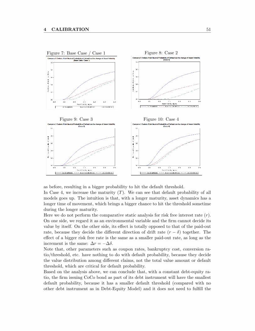
4 CALIBRATION 51

Figure 7: Base Case / Case 1 Figure 8: Case 2

Figure 9: Case 3 Figure 10: Case 4

as before, resulting in a bigger probability to hit the default threshold.In Case 4, we increase the maturity (T ). We can see that default probability of allmodels goes up. The intuition is that, with a longer maturity, asset dynamics has alonger time of movement, which brings a bigger chance to hit the threshold sometimeduring the longer maturity.Here we do not perform the comparative static analysis for risk free interest rate (r).On one side, we regard it as an environmental variable and the firm cannot decide itsvalue by itself. On the other side, its effect is totally opposed to that of the paid-outrate, because they decide the different direction of drift rate (r − δ) together. Theeffect of a bigger risk free rate is the same as a smaller paid-out rate, as long as theincrement is the same: ∆r = −∆δ.Note that, other parameters such as coupon rates, bankruptcy cost, conversion ra-tio/threshold, etc. have nothing to do with default probability, because they decidethe value distribution among different claims, not the total value amount or defaultthreshold, which are critical for default probability.Based on the analysis above, we can conclude that, with a constant debt-equity ra-tio, the firm issuing CoCo bond as part of its debt instrument will have the smallestdefault probability, because it has a smaller default threshold (compared with noother debt instrument as in Debt-Equity Model) and it does not need to fulfill the

4 CALIBRATION 52

debt payment responsibility after CoCo converts (compared with subordinate debtinstead). So from the perspective of default probability, CoCo bond would be a goodsecurity to keep the firm financially stable.

4.2 Risk Shifting Motivation

In this subsection, we consider the role of securities in mitigating the executive’spossible motivation to shift the firm’s asset risk.We assume that the dominant component of the executive payment package that issensitive to asset risk is equity-based compensation. In the common model setting,it is always assumed that executive will choose the level of asset risk that maximizesthe stock value to increase this part of compensation, rather than a risk level thatmeets the technology needs of the firm and would increase the firm’s future assetvalue (we call it optimal asset risk). In more detail, in cases where the equity value ismonotonically upward (or downward) sloping with respect to asset risk, the executivewill choose the maximum (or minimum) possible risk to maximize the value of theircompensation.Firstly we need to make it clear that how the asset risk level is decided amongexecutive and stakeholders of the firm. Executive will choose a risk level after theissuance of the securities, meaning that they can either increase or decrease risk fromits optimal level, given the capital structure and issued contract terms. Knowingtheir motivation, the firm’s stakeholders have to choose a capital structure and decidecontract terms to keep the equity value as stable as possible with different risk level,in order to prevent the executive from changing the risk level for their own benefit.If the stakeholder can successfully make this design, executive will not have themotivation to choose a risk level for their own benefit. Instead, they will choose arisk level that meets the technology needs of the firm and thus increases the firm’sfuture asset value, i.e. choosing the optimal risk level.So what we need to do is clear now. For the firm’s overall benefit, we will think of theproblem from the side of the stakeholders. So we will check whether it is possible tochange some contract terms of each model above to keep the equity value stable withdifferent risk level. Note that, compared with other terms, some contract terms arerigid and relatively more difficult to change as much as what we want. Reasons maycome from the firm’s former regulation, other considerations than the executive’s riskshifting motivation, or some contract parameters that are decided endogenously, etc.The firm’s asset risk is reflected by the asset volatility σ, and the expression of themarket value of equity in each model is already got in Section 3. We will begin thissubsection by studying the possible relationship of equity value and volatility in eachmodel with mathematical logic. Since the expression is quite complicated, we willdo the data calibration later to show it in a more straightforward way and hope thecalibration can meet our mathematical conclusion.In order to demonstrate this problem clearly, different from Section 4.1, we willinclude and start from the Benchmark Model. The conclusion from BenchmarkModel is where the traditional and classical theory comes from and thus it is worth

4 CALIBRATION 53

our attention.

4.2.1 Mathematical derivation

As in Section 4.1.1, we begin the comparison by mathematical derivation. All 4 mod-els are considered this time.

Benchmark ModelFrom the expression of the market value of equity (46), we can get its first orderderivative to volatility. If we regard equity in this model as a European Vanilla calloption, this first-order derivative is usually called the V ega (ν) of the call option, onekind of Greek Letters. We can easily get:

∂W0

∂σ= A0Φ

′(d1)∂(d1 − d2)

∂σ= A0φ(d1)

√T > 0 (188)

Φ(·) and φ(·) are the CDF and PDF of standard normal distribution.This derivative result is always strictly positive in all conditions. The economic in-tuition is that, with a higher volatility, equity holders have a bigger chance to get abigger repayment at maturity, while the protective function of call option guaranteesthat the biggest lost stays the same with a higher volatility.

Debt-Equity ModelUnlike the Benchmark Model, in the following models, we will not write out theexpression of the first order derivative of equity value to volatility, since the expres-sion is very long and not easy to judge its positive/negative sign. Instead, we willdemonstrate the intuition behind and verify our intuition by data calibration. The“price” is that we can just analyze the common conditions and have to leave awaysome extreme conditions with extreme parameter values. So what we provide belowis just a “rough” estimative analysis.In Debt-Equity Model, from (64), we can study the effect by dividing equity valueinto 2 compositions, J5 and J6. We see the effect of volatility on each compositionand then sum them up.From (62), J5 is monotonously negatively proportional to volatility. From (16), theexpectation of AT has nothing to do with volatility. But for the indicator function(1 if NO default), with a bigger volatility, its expectation (i.e. the probability of NOdefault) will become smaller. So we can conclude J5 is negatively proportional to σ.From (63), the direction of J6 is closely related to the sign of (δAs − c1D), i.e. posi-tive dividend or negative dividend payment. We roughly believe it is decided by therelationship of δ and c1, based on the fact that At and D are much closer to eachother in proportion (not absolute difference) than δ and c1. With a bigger volatili-ty, default time τd tends to be smaller and thus the upper bound of the integral isexpected to be smaller. If δ > c1, δAs − c1D > 0. It means less positive dividendpayment, so J6 is negatively proportional to σ. If δ < c1, it means less cost of raisingequity, so J6 is positively proportional to σ.

4 CALIBRATION 54

From both parts, we can roughly estimate that, if δ > c1 (positive dividend pay-ment), equity value in this model is negatively proportional to volatility; if δ < c1(negative dividend payment), two compositions of its value will partly offset andthe result depends on which part takes the “lead”. This estimation will be verifiedlater by comparing Figure 11 (Base Case) and Figure 15 (Case 3) via data calibration.

Subordinate Debt ModelIn this model, from (101), we can study the effect by dividing equity value into 3parts, J8, J9 and J10. We see the effect of volatility on each part and then sumthem up.From (95), J8 is monotonously negatively proportional to volatility. It is similar tothe analysis of J5 in Debt-Equity Model. For the indicator function (1 if NO defaultor conversion), with a bigger volatility, its expectation (i.e. the probability of NOconversion) will become smaller. So we can conclude J8 is negatively proportionalto σ.From (96), the direction of J9 is decided by 2 terms. The effect on max(·) is exactlythe same as the Benchmark Model, which is positively proportional to σ. But theeffect on the indicator function (1 if the minimum asset value locates between thedepression threshold and default threshold) is not monotonous. If the volatility istoo small, the changing of At is too little to pull it down and hit the buffer. If thevolatility is too big, the changing of At is dramatic and it can easily hit the defaultthreshold. So both extreme values of volatility make the expectation very small andactually it is an inverse “U” shape, meaning that the expectation of the indicatorfunction (i.e. the probability of that event) is positively proportional to volatility atthe beginning, and it will change to be negatively proportional later. The turningposition of volatility that makes the expecation biggest depends on the size of thebuffer and the distance from the initial asset value to the buffer. Based on the above2 terms, the relation of J9 and σ can be both sides.From (100), the direction of J10 looks more complicated and it is also not monotonous.Similar to the analysis of J6 in Debt-Equity Model, the value of δ and c1 matters(c2 is relatively not that important since S is much smaller than At or D under ourparameter assumption). While the integral bound becomes more complicated. Forthe second integral, its upper bound and lower bound both become smaller and theirrelationship is somewhat similar to the indicator function in J9 above. So its direc-tion depends not only on δ and c1, but also on the value of A0 and both thresholds.From 3 parts, we cannot have a clear conclusion about the relationship of equityvalue and volatility. We can just conclude that it is not monotonous and depends onthe parameter setting. This conclusion will be verified later by comparing Figure 11(Base Case) and Figure 17 (Case 4) via data calibration.

CoCo Bond ModelFor this model, the analysis is very similar to that of the Subordinate Debt Model.We just briefly give the conclusion here.From (146), we also study the effect by dividing equity value into 3 compositions,

4 CALIBRATION 55

J9, J10 and J11.From (140), J9 is monotonously negatively proportional to volatility.From (141), the direction of J10 is decided by the indicator function (1 if the minimumasset value locates between the conversion threshold and default threshold). But asbefore, it is not monotonous.From (145), the direction of J11 is also not monotonous.From 3 parts, we cannot have a clear conclusion about the relationship of equity valueand volatility. As before, we can just conclude that it is not monotonous and dependson our parameter setting. This conclusion will be verified by comparing Figure 12(Base Case) with Figure 14, 16 and 18 (Case 2, 3 and 4) via data calibration.

4.2.2 Calibrating the models

To make it more straightforward, we calibrate the models with assumed parametervalues under specified restrictions. We choose Base Case (as our Case 1) parametervalues and then perform comparative static analysis by changing one parameter valuein each case. We will check how asset volatility affects equity market value in eachmodel by setting it at the horizontal axis across the equity value at the verticalaxis. In this subsection’s calculation, on the basic of Table 10, we have to set somemore parameter values: the exogenously decided coupon rate of each debt instrument(corporate senior debt, subordinate debt and CoCo bond) and conversion threshold β.Bankruptcy cost parameter is still not needed because it just affects the market valueof corporate debt. In order to see the different effects on risk shifting motivation foreach model, we assume that the coupon rate of corporate debt c1 is the same across 3models, and the coupon rate of subordinate debt is equivalent to that of CoCo bond:

c2 = c3 (189)

Parameter setting for Base Case and 3 other cases is listed in Table 11. When plottingthe models, we put the plot of the first 3 models together in one figure, and the plotof CoCo Bond Model with different conversion ratios (α) in another figure. Figure11, 13, 15, 17 outline the market value of equity of the first 3 models, as the change ofasset volatility, based on the parameter value from Base Case (Case 1), Case 2, Case3 and Case 4 accordingly. Correspondingly, Figure 12, 14, 16, 18 is for the CoCoBond Model with different conversion ratios.All Figures above confirm our mathematical analysis in Section 4.2.1 about the rela-tionship between equity value and volatility for all 4 models. For benchmark model,it is strictly positively proportional, which proves the traditional theory of equity-volatility relationship under a perfect market setting. For 3 other models, we confirmthat the relationship can be positive as well as negative. Actually our data calibra-tion also verifies the non-monotonous relationship for each part of equity compositionwith volatility, such as J9, J10 in Subordinate Debt Model and J10, J11 in CoCoBond Model. Since they are just parts of the equity value and relatively not thatimportant in our analysis, we do not display their figures in this paper.Now we perform the comparative static analysis by comparing 3 other cases with the

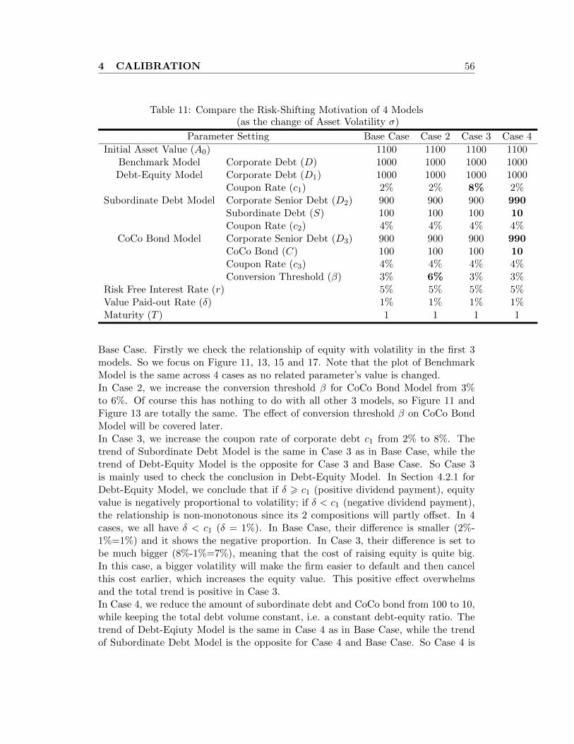
4 CALIBRATION 56

Table 11: Compare the Risk-Shifting Motivation of 4 Models(as the change of Asset Volatility σ)

Parameter Setting Base Case Case 2 Case 3 Case 4

Initial Asset Value (A0) 1100 1100 1100 1100Benchmark Model Corporate Debt (D) 1000 1000 1000 1000Debt-Equity Model Corporate Debt (D1) 1000 1000 1000 1000

Coupon Rate (c1) 2% 2% 8% 2%Subordinate Debt Model Corporate Senior Debt (D2) 900 900 900 990

Subordinate Debt (S) 100 100 100 10Coupon Rate (c2) 4% 4% 4% 4%

CoCo Bond Model Corporate Senior Debt (D3) 900 900 900 990CoCo Bond (C) 100 100 100 10Coupon Rate (c3) 4% 4% 4% 4%Conversion Threshold (β) 3% 6% 3% 3%

Risk Free Interest Rate (r) 5% 5% 5% 5%Value Paid-out Rate (δ) 1% 1% 1% 1%Maturity (T ) 1 1 1 1

Base Case. Firstly we check the relationship of equity with volatility in the first 3models. So we focus on Figure 11, 13, 15 and 17. Note that the plot of BenchmarkModel is the same across 4 cases as no related parameter’s value is changed.In Case 2, we increase the conversion threshold β for CoCo Bond Model from 3%to 6%. Of course this has nothing to do with all other 3 models, so Figure 11 andFigure 13 are totally the same. The effect of conversion threshold β on CoCo BondModel will be covered later.In Case 3, we increase the coupon rate of corporate debt c1 from 2% to 8%. Thetrend of Subordinate Debt Model is the same in Case 3 as in Base Case, while thetrend of Debt-Equity Model is the opposite for Case 3 and Base Case. So Case 3is mainly used to check the conclusion in Debt-Equity Model. In Section 4.2.1 forDebt-Equity Model, we conclude that if δ > c1 (positive dividend payment), equityvalue is negatively proportional to volatility; if δ < c1 (negative dividend payment),the relationship is non-monotonous since its 2 compositions will partly offset. In 4cases, we all have δ < c1 (δ = 1%). In Base Case, their difference is smaller (2%-1%=1%) and it shows the negative proportion. In Case 3, their difference is set tobe much bigger (8%-1%=7%), meaning that the cost of raising equity is quite big.In this case, a bigger volatility will make the firm easier to default and then cancelthis cost earlier, which increases the equity value. This positive effect overwhelmsand the total trend is positive in Case 3.In Case 4, we reduce the amount of subordinate debt and CoCo bond from 100 to 10,while keeping the total debt volume constant, i.e. a constant debt-equity ratio. Thetrend of Debt-Eqiuty Model is the same in Case 4 as in Base Case, while the trendof Subordinate Debt Model is the opposite for Case 4 and Base Case. So Case 4 is

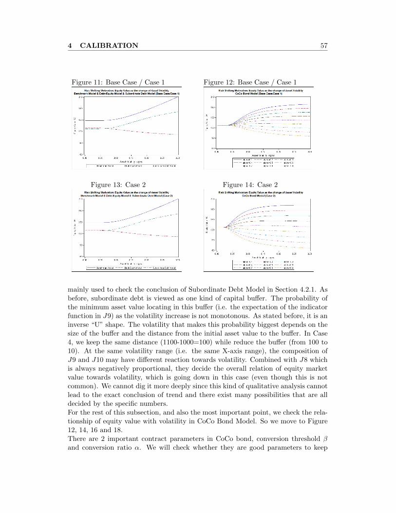
4 CALIBRATION 57

Figure 11: Base Case / Case 1 Figure 12: Base Case / Case 1


mainly used to check the conclusion of Subordinate Debt Model in Section 4.2.1. Asbefore, subordinate debt is viewed as one kind of capital buffer. The probability ofthe minimum asset value locating in this buffer (i.e. the expectation of the indicatorfunction in J9) as the volatility increase is not monotonous. As stated before, it is aninverse “U” shape. The volatility that makes this probability biggest depends on thesize of the buffer and the distance from the initial asset value to the buffer. In Case4, we keep the same distance (1100-1000=100) while reduce the buffer (from 100 to10). At the same volatility range (i.e. the same X-axis range), the composition ofJ9 and J10 may have different reaction towards volatility. Combined with J8 whichis always negatively proportional, they decide the overall relation of equity marketvalue towards volatility, which is going down in this case (even though this is notcommon). We cannot dig it more deeply since this kind of qualitative analysis cannotlead to the exact conclusion of trend and there exist many possibilities that are alldecided by the specific numbers.For the rest of this subsection, and also the most important point, we check the rela-tionship of equity value with volatility in CoCo Bond Model. So we move to Figure12, 14, 16 and 18.There are 2 important contract parameters in CoCo bond, conversion threshold βand conversion ratio α. We will check whether they are good parameters to keep

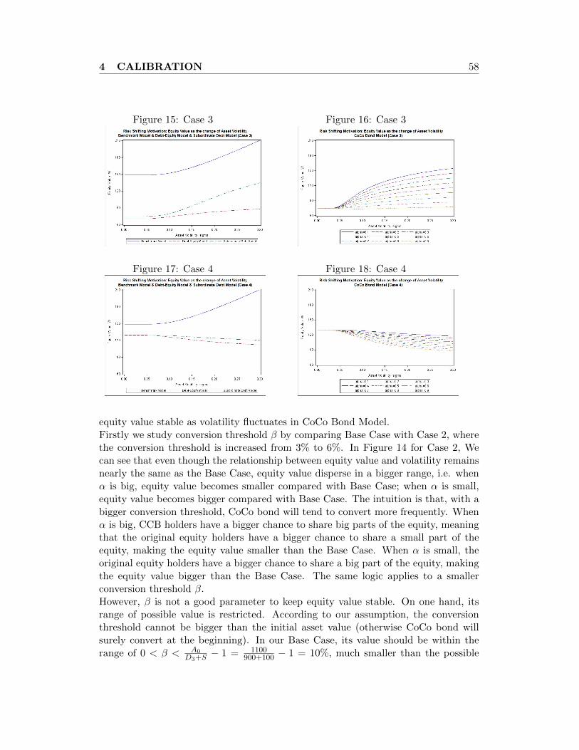
4 CALIBRATION 58



equity value stable as volatility fluctuates in CoCo Bond Model.Firstly we study conversion threshold β by comparing Base Case with Case 2, wherethe conversion threshold is increased from 3% to 6%. In Figure 14 for Case 2, Wecan see that even though the relationship between equity value and volatility remainsnearly the same as the Base Case, equity value disperse in a bigger range, i.e. whenα is big, equity value becomes smaller compared with Base Case; when α is small,equity value becomes bigger compared with Base Case. The intuition is that, with abigger conversion threshold, CoCo bond will tend to convert more frequently. Whenα is big, CCB holders have a bigger chance to share big parts of the equity, meaningthat the original equity holders have a bigger chance to share a small part of theequity, making the equity value smaller than the Base Case. When α is small, theoriginal equity holders have a bigger chance to share a big part of the equity, makingthe equity value bigger than the Base Case. The same logic applies to a smallerconversion threshold β.However, β is not a good parameter to keep equity value stable. On one hand, itsrange of possible value is restricted. According to our assumption, the conversionthreshold cannot be bigger than the initial asset value (otherwise CoCo bond willsurely convert at the beginning). In our Base Case, its value should be within therange of 0 < β < A0

D3+S− 1 = 1100

900+100 − 1 = 10%, much smaller than the possible

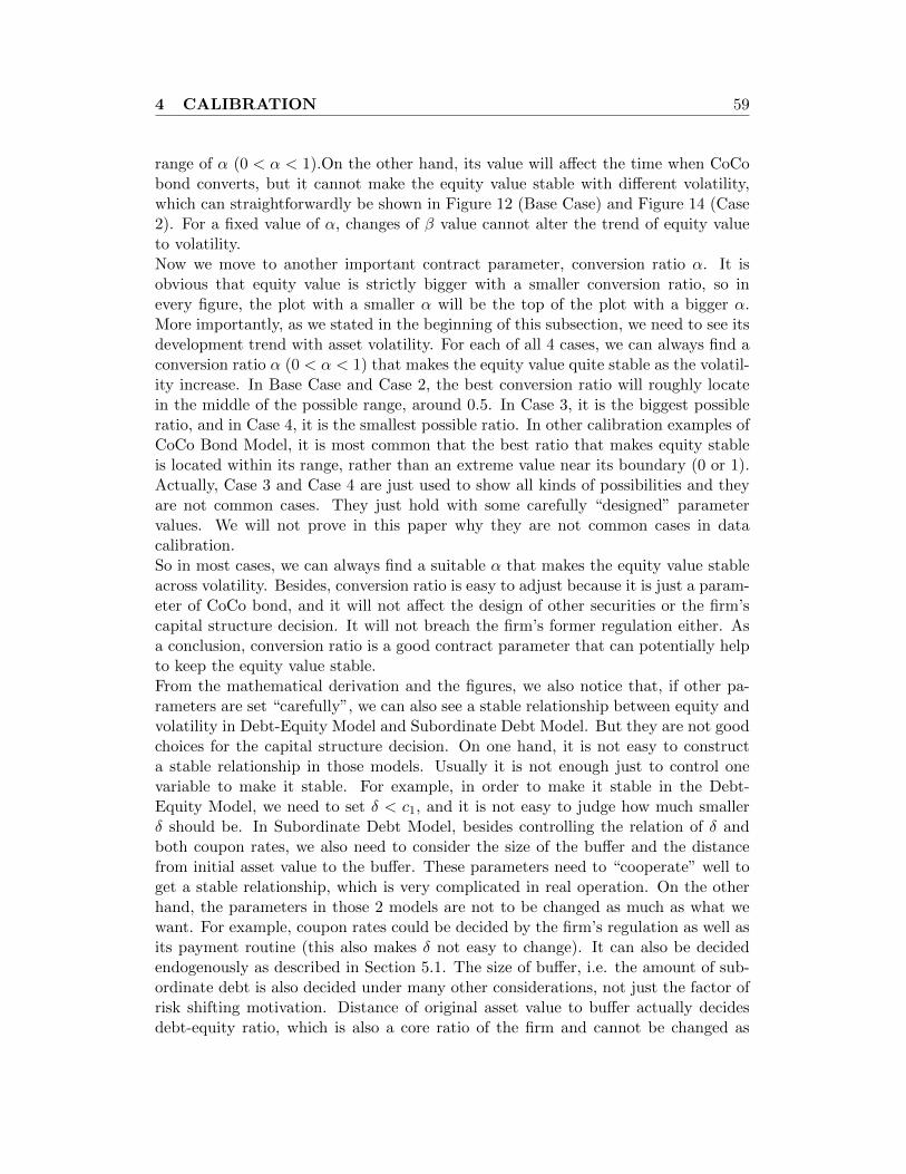
4 CALIBRATION 59

range of α (0 < α < 1).On the other hand, its value will affect the time when CoCobond converts, but it cannot make the equity value stable with different volatility,which can straightforwardly be shown in Figure 12 (Base Case) and Figure 14 (Case2). For a fixed value of α, changes of β value cannot alter the trend of equity valueto volatility.Now we move to another important contract parameter, conversion ratio α. It isobvious that equity value is strictly bigger with a smaller conversion ratio, so inevery figure, the plot with a smaller α will be the top of the plot with a bigger α.More importantly, as we stated in the beginning of this subsection, we need to see itsdevelopment trend with asset volatility. For each of all 4 cases, we can always find aconversion ratio α (0 < α < 1) that makes the equity value quite stable as the volatil-ity increase. In Base Case and Case 2, the best conversion ratio will roughly locatein the middle of the possible range, around 0.5. In Case 3, it is the biggest possibleratio, and in Case 4, it is the smallest possible ratio. In other calibration examples ofCoCo Bond Model, it is most common that the best ratio that makes equity stableis located within its range, rather than an extreme value near its boundary (0 or 1).Actually, Case 3 and Case 4 are just used to show all kinds of possibilities and theyare not common cases. They just hold with some carefully “designed” parametervalues. We will not prove in this paper why they are not common cases in datacalibration.So in most cases, we can always find a suitable α that makes the equity value stableacross volatility. Besides, conversion ratio is easy to adjust because it is just a param-eter of CoCo bond, and it will not affect the design of other securities or the firm’scapital structure decision. It will not breach the firm’s former regulation either. Asa conclusion, conversion ratio is a good contract parameter that can potentially helpto keep the equity value stable.From the mathematical derivation and the figures, we also notice that, if other pa-rameters are set “carefully”, we can also see a stable relationship between equity andvolatility in Debt-Equity Model and Subordinate Debt Model. But they are not goodchoices for the capital structure decision. On one hand, it is not easy to constructa stable relationship in those models. Usually it is not enough just to control onevariable to make it stable. For example, in order to make it stable in the Debt-Equity Model, we need to set δ < c1, and it is not easy to judge how much smallerδ should be. In Subordinate Debt Model, besides controlling the relation of δ andboth coupon rates, we also need to consider the size of the buffer and the distancefrom initial asset value to the buffer. These parameters need to “cooperate” well toget a stable relationship, which is very complicated in real operation. On the otherhand, the parameters in those 2 models are not to be changed as much as what wewant. For example, coupon rates could be decided by the firm’s regulation as well asits payment routine (this also makes δ not easy to change). It can also be decidedendogenously as described in Section 5.1. The size of buffer, i.e. the amount of sub-ordinate debt is also decided under many other considerations, not just the factor ofrisk shifting motivation. Distance of original asset value to buffer actually decidesdebt-equity ratio, which is also a core ratio of the firm and cannot be changed as

5 EXTENSIONS 60

much as we want.Instead, in CoCo Bond Model, without considering other parameters, at least wehave the parameter of conversion ratio α which can easily make the equity valuestable by itself in most cases. Besides, its value is easy to control and adjust becauseit is just a contract term of CoCo bond, as stated above. We even do not need tochange other CoCo bond contract parameters (such as β). Because of this property,CoCo Bond Model is the best model for the consideration of mitigating executive’srisk shifting motivation.

5 Extensions

In this section, we will make some extensions by changing the model setting andassumptions. This is a useful attempt because the security design in real financialworld may take some different forms and a standard model cannot explain all kind-s of security design. Besides, it examines the model from another perspective anddeepens our understanding of the original model.We will just make the extension for the CoCo Bond Model in this section. On oneside, the design, valuation and application of CoCo bond is the core in this paper.Other supporting models are introduced and designed just for comparison with thecore model, as what we did in Section 4. On the other side, the extensions can beapplied in a very similar way to other models in this paper with the same logic.

5.1 Endogenous coupon rates

In the above models with debts that pay coupons, we assume that their coupon ratesc1, c2 and c3 are exogenous. Under the exogenous coupon rate assumption, couponrate can take any “reasonable” value, which can be bigger or smaller than the riskfree interest rate. From Section 3, we know that their selected values can have a bigeffect on the market value of claims. If we assume the coupon rates are endogenouslydecided, then how can it be decided within the model?In an efficient financial market, the issuing price of the debt and its coupon rates aremutually reflective in information. For example, if a firm set a higher coupon ratec1 for its senior corporate debt, from (129) we know that its initial market value D0

will be higher. According to the arbitrage-free pricing theorem, the issuing price ofa security will be its initial market value. So with a higher c1, the issuing price ishigher and may higher than its face value D. At this time, we will say that this debtis selling over par, meaning the issuing price is over its par value, i.e. face value.The same logic applies to a lower c1 that may leads to a lower issuing price than itspar value, which is called issuing under par. The coupon rate that makes the issuingprice equal to its face value is actually its yield to maturity. So here, we assumethe coupon rate of senior corporate debt (CoCo bond) is its yield to maturity whichmakes its initial market value D0 (CCB0) equal to its face value D (C). This is agood attempt. Coupon rates decided in this way is infomative since they carry the

5 EXTENSIONS 61

securities’ risk information. It can be used to compare with the risk free interest rateand measure the risk of the security in a quantitative way. The fair spread of debt iscalculated in this way by deducting risk free interest rate from its fair coupon rate.So in this extension of the CoCo Bond Model, we just need the changes of settingboth coupon rates c1 and c3 as unknown and having 2 more restrictive conditions.

D0 = D (190)

CCB0 = C (191)

Mathematically it is easy to do the rest of the valuation work.From (129) and (132), we can get c1:

c1 =D − EQ[J2 + J3]∫ min(τd,T )0 e−rsD ds

(192)

From (135) and (139), we can get c3:

c3 =C − EQ[J6 + J7 + J8(c1)]∫ min(τc,T )

0 e−rsC ds(193)

Now we can get the endogenously decided coupon rates c1 and c3.With these endogenous coupon rates, we can calculate the initial market value ofequity as:

W0 = EQ[J9 + J10 + J11(c1, c3)] (194)

We can easily verify Asset Equation (128) which takes the form here as:

A0 = D +BC0 + C +W0 (195)

What we are interested in this extension is the coupon rates of both debts becausethey carry the risk information of both debts. As in Section 4, we utilize the calibra-tion method. We calibrate this extension with the parameter values of Base Case andCase 2 defined in Table 10. For calculation, we also need the conversion threshold βto decide the conversion trigger. We take it from the Base Case in Table 11 (β = 3%).Besides, we also need to define one more parameter value: bankruptcy cost ω. Weset it as ω = 0.4 here. As before, we set the volatility at the horizontal axis, acrossboth coupon rates at the vertical axis.Parameter value in Figure 19 is from the Base Case in Table 10 (adding β = 3% andω = 0.4). In Figure 20, we just change the firm’s debt structure by increasing theface value of CoCo bond while keeping the total debt volume constant (data fromCase 2 in Table 10), i.e. a constant debt-equity ratio.For the fair coupon rate of corporate debt c1, it is always bigger than risk free interestrate, and it becomes bigger and bigger as the volatility increases. This meets ourintuition. With a bigger volatility, corporate debt holders cannot get more than thedebt’s face value at maturity if the asset value goes up, and they have a bigger chance

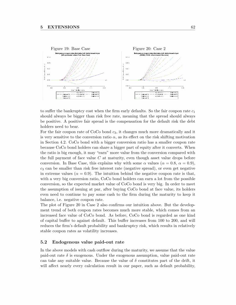
5 EXTENSIONS 62

Figure 19: Base Case Figure 20: Case 2

to suffer the bankruptcy cost when the firm early defaults. So the fair coupon rate c1should always be bigger than risk free rate, meaning that the spread should alwaysbe positive. A positive fair spread is the compensation for the default risk the debtholders need to bear.For the fair coupon rate of CoCo bond c3, it changes much more dramatically and itis very sensitive to the conversion ratio α, as its effect on the risk shifting motivationin Section 4.2. CoCo bond with a bigger conversion ratio has a smaller coupon ratebecause CoCo bond holders can share a bigger part of equity after it converts. Whenthe ratio is big enough, it may “earn” more value from the conversion compared withthe full payment of face value C at maturity, even though asset value drops beforeconversion. In Base Case, this explains why with some α values (α = 0.8, α = 0.9),c3 can be smaller than risk free interest rate (negative spread), or even get negativein extreme values (α = 0.9). The intuition behind the negative coupon rate is that,with a very big conversion ratio, CoCo bond holders can earn a lot from the possibleconversion, so the expected market value of CoCo bond is very big. In order to meetthe assumption of issuing at par, after buying CoCo bond at face value, its holderseven need to continue to pay some cash to the firm during the maturity to keep itbalance, i.e. negative coupon rate.The plot of Figure 20 in Case 2 also confirms our intuition above. But the develop-ment trend of both coupon rates becomes much more stable, which comes from anincreased face value of CoCo bond. As before, CoCo bond is regarded as one kindof capital buffer to against default. This buffer increases from 100 to 200, and willreduces the firm’s default probability and bankruptcy risk, which results in relativelystable coupon rates as volatility increases.

5.2 Endogenous value paid-out rate

In the above models with cash outflow during the maturity, we assume that the valuepaid-out rate δ is exogenous. Under the exogenous assumption, value paid-out ratecan take any suitable value. Because the value of δ constitutes part of the drift, itwill affect nearly every calculation result in our paper, such as default probability,

5 EXTENSIONS 63

market value of claims, endogenous coupon rate, etc. If we assume the value paid-outrate is endogenously decided, then how can it be decided within the model?As in the above extension, we need more restriction or assumption to decide thevalue of endogenous variable. In CoCo bond model, the model can be internallyconsistent (i.e. the fulfillment of Asset Equation) with an exogenous value paid-outrate. That is because of the existence of equity dividend and we leave all the rest ofthe intermediate paid-out value (positive or negative) to equity holders as dividendafter any coupon responsibility. So, if we assume that the firm does not pay out anydividend during the maturity, the value paid-out rate can no longer be exogenous.The assumption of non-dividend payment in this extension is reasonable because inreal financial market, especially during the financial crisis, many firms choose notto pay any dividend or just pay very little dividend to their equity holders. Ourextension here outlines the behaviors of this kind of behavior.A new restriction is needed to calculate the endogenous δ. And this restriction shouldalso makes the model internally consistent (i.e. the fulfillment of Asset Equation) aswell. Compared with (148), we have the following restriction:

EQ[∫ min(τd,T )

0e−rsδAs ds

]= EQ[J1 + J5]


0e−rsc1D ds+

∫ min(τc,T )

0e−rsc3C ds

](196)

This restriction condition indicates that, the present value of all values paid outduring the maturity is equal to the present value of both types of coupon payment.Without dividend payment, J18 and J11 in (148) no longer exist. Value paid outduring each time interval δAt dt all goes to the coupon payment of senior debt andCoCo bond.Note again that the left hand side should be the expectation of

∫ min(τd,T )0 e−rsδAs ds,

rather than∫ T0 e−rsδAs ds, because the firm will be taken over and will not pay out

any value after it hits the default threshold at time τd.For other parts of calculation, it is nearly the same as the original model. We justneed to skip away the dividend payment of J8 and J11, and thus (139) and (146)becomes:

CCB0 = EQ[J5 + J6 + J7] (197)

W0 = EQ[J9 + J10] (198)

We can also easily verify Asset Equation (128), with (148) replaced by (196) andother parts remaining the same.Actually the valuation becomes easier if we can achieve the endogenous δ value be-cause the mathematical derivation of dividend payment in the original model is verycomplicated and here we do not need to take dividend payment into consideration.So the only problem now is how to achieve δ from (196).Even though we have got the explicit expression of both sides of (196) (left hand sidefrom (79) and right hand side from (154), (158)), we cannot write out the expression

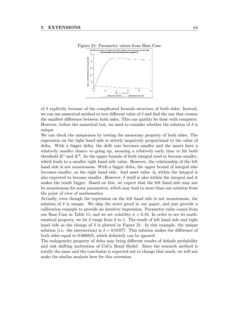
5 EXTENSIONS 64

Figure 21: Parameter values from Base Case

of δ explicitly because of the complicated formula structure of both sides. Instead,we can use numerical method to test different value of δ and find the one that createsthe smallest difference between both sides. This can quickly be done with computer.However, before the numerical test, we need to consider whether the solution of δ isunique.We can check the uniqueness by testing the monotony property of both sides. Theexpression on the right hand side is strictly negatively proportional to the value ofdelta. With a bigger delta, the drift rate becomes smaller and the assets have arelatively smaller chance to going up, meaning a relatively early time to hit boththreshold Kc and Kd. So the upper bounds of both integral tend to become smaller,which leads to a smaller right hand side value. However, the relationship of the lefthand side is not monotonous. With a bigger delta, the upper bound of integral alsobecomes smaller, as the right hand side. And asset value At within the integral isalso expected to become smaller. However, δ itself is also within the integral and itmakes the result bigger. Based on this, we expect that the left hand side may notbe monotonous for some parameters, which may lead to more than one solution fromthe point of view of mathematics.Actually, even though the expression on the left hand side is not monotonous, thesolution of δ is unique. We skip the strict proof in our paper, and just provide acalibration example to provide an intuitive impression. Parameter value comes fromour Base Case in Table 11, and we set volatility σ = 0.10. In order to see its math-ematical property, we let δ range from 0 to 1. The result of left hand side and righthand side as the change of δ is plotted in Figure 21. In this example, the uniquesolution (i.e. the intersection) is δ = 0.01877. This solution makes the difference ofboth sides equal to 0.000825, which definitely can be ignored.The endogeneity property of delta may bring different results of default probabilityand risk shifting motivation of CoCo Bond Model. Since the research method istotally the same and the conclusion is expected not to change that much, we will notmake the similar analysis here for this extension.

6 SUMMARY 65

6 Summary

In this paper, we develop a structural model to value Contingent Convertible Bond, adebt instrument that automatically converts to equity if the issuing institution suffersfinancial distress. Our model is based on a long line of research on capital structureby some classical option pricing papers. We derive close-form formula for the marketvalue of CoCo bond when the institution’s asset value is modeled as a GeometricBrownian Motion process and its conversion trigger is set as a threshold of assetvalue. The key distinguishing feature of our model is that we design the bonds ascoupon-paid with finite maturity, which makes this security more implementable inreal financial world. This is also the first attempt in literatures that use asset valueas CoCo bond’s conversion trigger. We also extend our analysis by showing thatthe institution’s intermediate value paid-out rate or bond coupon rates can be set asendogenous, which is also an innovative attempt in the literature of CoCo bond. Inthe data calibration section, we prove that the introduction of CoCo bond into thecapital structure, compared with introducing subordinate debt or nothing, can alwaysreduce the institution’s default probability and effectively mitigate the management’srisk shifting motivation. Our paper shows the significance of contingent capital inenhancing the financial stability of large financial institutions, especially in a wellfluctuating financial environment.

7 REFERENCE 66

7 Reference

Albul, B., Jaffee, D. M., and Tchistyi, A. 2010, ‘Contingent Convertible Bonds andCapital Structure Decisions’, working paper, University of California, Berkeley

Black, F., and Cox, J.C. 1976, ‘Valuing Corporate Securities: Some effects of BondIndenture Provisions’, Journal of Finance 31, 351-367

Black, F., and Scholes, M. 1973, ‘The pricing of options and corporate liabilities’,Journal of Political Economy 81, 637-654

Duffie, D. 2001, Dynamic Asset Pricing Theory, 3rd ed., Princeton University Press

Duffie, D. 2010, ‘A Contractual Approach to Restructuring Financial Institutions’,in K.B. Scott, G.P. Shultz, and J.B. Taylor eds., Ending government bailouts as weknow them, Hoover Press

Flannery, M.J. 2005, ‘No Pain, No Gain? Effecting Market Discipline via ReverseConvertible Debentures’, in H.S. Scott (ed.), Capital Adequacy Beyond Basel: Bank-ing, Securities, and Insurance, Oxford University Press

Flannery, M.J. 2009, ‘Stabilizing Large Financial Institution with Contingent CapitalCertificates’, working paper, University of Florida

Flannery, M.J. 2009, ‘Market-value triggers will work for contingent capital instru-ments’, Solicited Submission to U.S. Treasury Working Group on Bank Capital

Glasserman, P., and Nouri, B. 2010, ‘Contingent Capital with a Capital-Ratio Trig-ger’, working paper, Columbia University

Glasserman, P., and Wang, Z. 2009, ‘Valuing the Treasury’s Capital Assistance Pro-gram’, Staff Report, Federal Reserve Bank of New York

Harrison, J.M. 1985, Brownian Motion and Stochastic Flow Systems, Wiley, NewYork

Hart, O., and Zingales, L. 2010, ‘A new capital regulation for large financial institu-tions’, working paper, University of Chicago

Kashyap, A.K., Rajan, R.G., and Stein, J.C. 2008, ‘Rethinking Capital Regulation’,working paper, Kansas City Symposium on Financial Stability

Leland, H.E. 1994, ‘Corporate Debt Value, Bond Covenants, and Optimal CapitalStructure’, Journal of Finance 49, 1213-1252

7 REFERENCE 67

Leland, H.E., and Toft, K.B. 1996, ‘Optimal Capital Structure, Endogenous bankrupt-cy, and the Term Structure of Credit Spreads’, Journal of Finance 51, 987-1019

McDonald, R. 2010, ‘Contingent Capital with a Dual Price Trigger’, working paper,Northwestern University

Merton, R.C. 1973, ‘The theory of rational option pricing’, Bell Journal of Economicsand Management Science, Vol. 4, No. 1

Merton, R.C. 1974, ‘On the pricing of Corporate Debt: The risk structure of interestrates’, Journal of Finance 29, 449-469

Pennacchi, G. 2010, ‘A Structural Model of Contingent Bank Capital’, working pa-per, Federal Reserve Bank of Cleveland

Pennacchi, G., Vermaelen, T., and Wolff, C.C.P. 2010, ‘Contingent Capital: The casefor COERCs’, working paper

Protter, P. 1990, Stochastic Integration and Differential Equations, Springer, NewYork

Raviv, A. 2004, ‘Bank Stability and Market Discipline: Debt-for-Equity Swap versusSubordinated Notes’, working paper, Hebrew University

Raviv, A. and Hilscher, J. 2011, ‘Bank Stability and market discipline: The effect ofcontingent capital on risk taking and default probability’, working paper, BrandeisUniversity

Squam Lake Working Group on Financial Regulation 2009, ‘An expedited resolutionmechanism for distressed financial firms: Regulatory Hybrid Securities’, working pa-per, Center for Geoeconomic Studies, Council in Foreign Relations

Sundaresan, S. and Wang, Z. 2010, ‘Design of Contingent Capital with a stock pricetrigger for mandatory conversion’, working paper, Federal Reserve Bank of New York

the Role of Contingent Convertible Bond in Capital...

Documents

Transcript of the Role of Contingent Convertible Bond in Capital...