UNIVERSITATEA POLITEHNICA TIMIS¸OARA · • Mircea Vladutiu(director), Mihai Udrescu (member),...
120
UNIVERSITATEA POLITEHNICA TIMIS ¸OARA Network Science in Computer Engineering and Information Technology Habilitation Thesis Mihai UDRESCU-MILOSAV 2017
Transcript of UNIVERSITATEA POLITEHNICA TIMIS¸OARA · • Mircea Vladutiu(director), Mihai Udrescu (member),...

UNIVERSITATEA POLITEHNICA TIMISOARA
Network Science in Computer
Engineering and Information Technology
Habilitation Thesis
Mihai UDRESCU-MILOSAV
2017

2

i
Acknowledgements
This thesis stems from my personal research efforts in the fields of complex networks,computer engineering, and algorithm design. However, along the way, this exciting re-search journey was influenced and supported by many. First, I want to thank my family:my wife Lucretia, my son Mihai Jr., and my parents Sorina and Mircea. Without theirunderstanding and unconditioned support, none of the contributions presented in thisthesis would have been possible. Then, I want to thank my mentors: my former PhDadvisor prof. Mircea Vladutiu from Politehnica University of Timisoara, and prof. RaduMarculescu of Carnegie Mellon University. Indeed, the best ideas presented in this the-sis can be traced back to my research visit at CMU, hosted by professor Marculescu’sresearch group in 2011; it was a period of hard and enthusiastic work, in which I wasalso guided by my good friend Paul Bogdan, who is now a professor at the Universityof Southern California. When I returned home, many of the seminal ideas from CMUfound fertile ground in Timisoara. I was lucky to have on my side all my friends and col-leagues from the Advanced Computing Systems and Architectures (ACSA) lab at UPT(Lucian Prodan, Alexandru Topırceanu, Alexandru Iovanovici, Cristian Ruican, FlaviusOpritoiu, Razvan Avram, Gabriel Barina, Constantina Gavriliu, Alexandra Duma), aswell as with my good friend and UPT postdoc Andrei Lihu. I developed some of theCMU ideas as applications in the field of precision medicine, by opening a fruitful collab-oration with dr. Stefan Dan Mihaicuta and his colleagues from University of Medicineand Pharmacy Timisoara (UMFT), with the pharmacists from the Faculty of Pharmacyat UMFT (Lucretia Udrescu, Laura Sbarcea, and Liana Suciu), as well as with prof.Ludovic Kurunczi from the Institute of Chemistry of the Romanian Academy. Thefield of network science has blessed me with the opportunity of finding new horizons forcomputing applications, and with the opportunity of discussing novel ideas with out-standing researchers in the fields of medicine and biochemistry, such as my friend IoanOvidiu Sırbu; his dedication for helping people through research is an unfailing source ofinspiration. Finally, I want to thank those who financed our research: Linde Healthcareand UEFISCDI.

ii

Contents
I Contributions v
1 Introduction 11.1 Motivation . . . . . . . . . . . . . . . . . . . . . . . . . . . . . . . . . . . 21.2 Research Path . . . . . . . . . . . . . . . . . . . . . . . . . . . . . . . . . 41.3 Contributions . . . . . . . . . . . . . . . . . . . . . . . . . . . . . . . . . 71.4 Complex Network Science . . . . . . . . . . . . . . . . . . . . . . . . . . 11
1.4.1 Basic Parameters . . . . . . . . . . . . . . . . . . . . . . . . . . . 111.4.2 Network Centralities . . . . . . . . . . . . . . . . . . . . . . . . . 131.4.3 Energy Layouts and Network Clustering . . . . . . . . . . . . . . 141.4.4 Network Models . . . . . . . . . . . . . . . . . . . . . . . . . . . . 14
1.5 Thesis Outline . . . . . . . . . . . . . . . . . . . . . . . . . . . . . . . . . 20
2 Social Network Analysis 232.1 Introduction . . . . . . . . . . . . . . . . . . . . . . . . . . . . . . . . . . 232.2 Probabilistic modeling of opinion spread models . . . . . . . . . . . . . . 25
2.2.1 3-state tolerance model . . . . . . . . . . . . . . . . . . . . . . . . 272.2.2 Tolerance model with 4 states . . . . . . . . . . . . . . . . . . . . 282.2.3 Experimental results . . . . . . . . . . . . . . . . . . . . . . . . . 30
2.3 Discussion and Conclusions . . . . . . . . . . . . . . . . . . . . . . . . . 35
3 Network Pharmacology and Network Medicine 373.1 Network Pharmacology . . . . . . . . . . . . . . . . . . . . . . . . . . . . 37
3.1.1 Drug-drug interaction network analysis . . . . . . . . . . . . . . . 383.1.2 Interpreting network centralities . . . . . . . . . . . . . . . . . . . 403.1.3 Results Interpretation . . . . . . . . . . . . . . . . . . . . . . . . 45
3.2 Network Medicine . . . . . . . . . . . . . . . . . . . . . . . . . . . . . . . 463.2.1 Processing Medical Databases . . . . . . . . . . . . . . . . . . . . 473.2.2 Network Analysis for OSAS Patients Phenotype Definition . . . . 523.2.3 Validation of OSAS Risk Prediction with SASScore . . . . . . . . 603.2.4 Discussion . . . . . . . . . . . . . . . . . . . . . . . . . . . . . . . 63
II Future Research Developments 69
4 On-Chip Communication Networks 71
iii

iv CONTENTS
4.1 Introduction . . . . . . . . . . . . . . . . . . . . . . . . . . . . . . . . . . 714.2 Background and Motivation . . . . . . . . . . . . . . . . . . . . . . . . . 72
4.2.1 State-of-the-Art . . . . . . . . . . . . . . . . . . . . . . . . . . . . 724.2.2 Perspectives . . . . . . . . . . . . . . . . . . . . . . . . . . . . . . 73
4.3 On-Chip Fractal Architectures . . . . . . . . . . . . . . . . . . . . . . . . 734.3.1 Topology Generation . . . . . . . . . . . . . . . . . . . . . . . . . 74
4.4 Resource Management in Fractal Networks . . . . . . . . . . . . . . . . . 794.4.1 Routing . . . . . . . . . . . . . . . . . . . . . . . . . . . . . . . . 794.4.2 Dimensioning of Communication Channels . . . . . . . . . . . . . 824.4.3 Surface Allocation . . . . . . . . . . . . . . . . . . . . . . . . . . 85
4.5 Conclusion . . . . . . . . . . . . . . . . . . . . . . . . . . . . . . . . . . . 88
5 Conclusions 91
III Relevant Bibliography 95

Part I
Contributions
v


Chapter 1
Introduction
Since the beginning of the new Millennia, we have witnessed the emergence of the NewNetwork Science, or the science of Complex Networks [4]; this new field is consideredas a stand-alone science although it encompass elements from physics, mathematics,and computer science (see Figure 1.1). Specifically, the science of Complex Networksdeals with the structure and behavior of complex systems that can be modelled asgraphs, namely mathematical structures consisting of objects, nodes, or vertices, whichare connected with lines, links, or edges. The fundamental difference between graphsfrom conventional graph theory and complex networks consists of the number of nodes(small for conventional graphs, up to several millions for complex networks) and theinterconnection topology (regular, Euclidian lattice for conventional graphs, as opposedto complex and irregular for complex networks).
Figure 1.1: A general overview on Network science, highlighting the convergence ofPhysics (Complex Systems), Mathematics (Graph Theory), and Computer Science andEngineering (Algorithms and Databases).
Although the field of Complex Networks is implicitly multidisciplinary, it is mostlyrelated to physics, specifically to statistical physics and complex systems. The prac-tical applications of such tremendous theoretical developments are extensive: biology,
1

2 CHAPTER 1. INTRODUCTION
medicine, economy, social sciences, engineering (including electrical engineering andcomputers), computer science, and physics. As such, considering the field of applica-tion, the vast domain of Complex Networks can be divided in:
• Biological networks: disease networks, food networks in given environments,gene networks, pathway networks, metabolic networks, protein interaction net-works, drug interaction networks, etc.
• Technological networks: computer networks, the world wide web, road andtransportation networks, power distribution networks, electronic components net-work, computer software class networks, etc.
• Social networks: online social networks, political networks, economic networks,friendship networks, collaboration networks, etc.
• Semantic networks: LISP semantic network, natural language word networks,etc.
As a consequence, technological complex network techniques and methodologies canbe used in Computer Engineering applications which entail a big amount of complexity[136]. At the same time, the overarching field of Information Technology includes variousapproaches where computer algorithms and applications are used for the advancement ofbiology, medicine, pharmacology, or social physics. Indeed, the last decade has witnessedsignificant progress in personalized or precision medicine, based on big data techniquesand computer technologies such as Complex Network Analysis, Machine Learning (in-cluding Deep Learning) [44]. Moreover, the advance in social system physics has gain alot of momentum since the global dissemination of Online Social Networks [5].
1.1 Motivation
Our main motivation in research is to find solutions for problems pertaining to com-puter engineering and information technology, by finding inspiration in physics. Assuch, our previous research, during the PhD program and the period 2004-2012 wasfocused on quantum computing, namely quantum algorithms, assessing and improvingthe reliability of quantum circuits.
Since 2012, after being exposed to the seminal ideas of the new science of complexnetworks, our research started to target the application of network science in computerengineering and information technology. As Figure 1.2 shows, the first application is inthe field of Computer Engineering. Specifically, our goal is to find efficient techniquesfor design space exploration of multi-core, networks on chip (NoC) computer architec-tures. One of the most critical aspects of such NoC systems is represented by inter-corecommunication traffic which is mediated by the on-chip network communication infras-tructure. The fact that the on-chip networks have regular topologies, as required byphysical circuit implementation technology, are making the NoC systems prone to datatraffic congestions. We propose fractal topologies for on-chip interconnection in NoCsystems as they can be both regular (therefore, amenable to physical implementation)

1.1. MOTIVATION 3
and efficient in alleviating data traffic congestions. Indeed, we prove the efficiency offractal NoC topologies by using the methods of complex network analysis.
Figure 1.2: Applications of Complex Network Science in Computer Engineering (NoCFractal Architectures) and Information Technology (Social Networks, Systems Pharma-cology, and Network Medicine).
The second application of complex network science targets the field of social net-works. As such, we analyze on of the most researched aspects in this field, namely opin-ion spread models [1][3]. We opted for using computer simulation as research method-ology to evaluate and test these opinion spread models in social networks, because amathematical analysis is not able to provide tools that cope with the huge complexityof social network topologies. For instance, in order to allow for mathematical anal-ysis some social network researchers use simple, regular topologies such as lattice orfully connected networks [3], while others use random networks as this type of complextopologies can be analyzed by using statistics [30]. Therefore, by using the increasedanalytical power of computer simulation we show that our new model of opinion inter-action and spreading in social network generates more realistic patterns. Our modelis inspired from the research of Acemoglu et al. [1][3] which assumes the presence ofso-called stubborn agents (i.e. social network agents which do not change their opinion)and that the degree of being influenced by other opinions is weighted by the trust factor,which is a fixed value assigned at the beginning of simulation for each social agent. Weadd to Acemoglu’s model a new type of agents, namely null agents who do not haveany opinion, as well as time variability in the trust factor which we call tolerance. Therules that govern the evolution of one agent’s tolerance toward other agents’ opinionsare inspired from social psychology [185].
We also applied network science in information technology by aiming at providingcomputer-based solutions for pharmacological and medical problems. One such approachuses the international public database drugbank.ca [205] in order to build a drug-druginteraction network, where nodes represent drugs whereas links represent drug-drug

4 CHAPTER 1. INTRODUCTION
interaction relationships between the drugs. By employing 2D force-directed layoutalgorithms [147] and modularity class clustering [144], we automatically segregate drugcommunities which can be associated to specific drug properties [190]. In turn, drugproperty associations discovered with our methodology can be employed for predictingnew interactions or for performing drug repositioning (repurposing) [171][123]. Themethodological framework which uses a dual clustering technique, namely energy-modellayouts and modularity classes, can also be used in other medical applications suchas finding patient phenotypes in order to foster personalized treatment and precisediagnostics. To this end, we used the aforementioned dual technique in order to defineprecision clusters in a large database of Obstructive Sleep Apnea Syndrome (OSAS)patients [120]. By analyzing the accurately described patient phenotypes, we are ableto introduce a new OSAS prediction score that achieves a drastically improved predictionspecificity with respect to the state of the art [192].
1.2 Research Path
Our PhD research activity was related to domains such as Quantum Computing, Com-puter Reliability, and Evolvable Hardware; this activity was supported by the followingresearch grants:
• Mihai Udrescu (director), Mircea Vladutiu, Oana Boncalo, Alexandru Amaricai,Virgil Petcu, Cristian Ruican, Nicolae Velciov. ”Fault Tolerant Design of Quantumand Reversible Circuits (Proiectarea Circuitelor Cuantice si Reversibile Tolerantela Defectare”, R&D Grant CNCSIS, Type A, 380/2007 (Total value: 159000 ROL)
• Mircea Vladutiu (director), Mihai Udrescu (member), Lucian Prodan, Oana Boncalo,Alexandru Amaricai, ”Bioinspired Computer Architectures for Reversible andQuantum Logic Circuits (Arhitecturi Bioinspirate de Calcul pentru Circuite LogiceReversibile si Cuantice)”, R&D Grant, PNII IDEI 17/2007 (Total value: 440000ROL)
• Mircea Vladutiu (Director), Mihai Udrescu, Lucian Prodan, Oana Boncalo, Alexan-dru Amaricai, Versavia Ancusa, Nicolae Velciov, Alin Anton, ”Bioinspired Designof Applications on Reconfigurable Platforms (Proiectarea Bioinspirata a Aplicati-ilor pe Platforme Reconfigurabile)”, R&D Grant, CNCSIS Type A 643/2005 (Totalvalue: 67800 ROL)
The main PhD research activity results, as well as results from our post-PhD ac-tivity prior to the Complex Network period were reported in the following (selected)publications:
• Books
B1 Mihai Udrescu, Lucian Prodan, Emerging Computing Systems: QuantumComputing From a Computer Engineering Perspective, in Colectia Calcu-latoare, Editura Politehnica, Timisoara, Romania, 2013, [128 pages], ISBN978-606-554-684-4.

1.2. RESEARCH PATH 5
B2 Mihai Udrescu, Quantum Circuits Engineering, in Colectia Calculatoare, Ed-itura Politehnica, Timisoara, Romania, 2009, [227 pages], ISBN 978-973-625-815-2
• Journal papers
J1 Mihai Udrescu, Lucian Prodan, Mircea Vladutiu, Simulated Fault InjectionMethodology for Gate-Level Quantum Circuit Reliability Assessment, Simu-lation Modelling Practice and Theory, 23, 1, 60–70, 2012 [IF=1.159, Q2 –Computer Science, Software Engineering]
J2 Oana Boncalo, Alexandru Amaricai, Mihai Udrescu, Mircea Vladutiu, Quan-tum Circuit’s Reliability Assessment with VHDL-Based Simulated Fault In-jection, Microelectronics Reliability, 50, 2, 304–311, 2010 [IF=1.137]
J3 Lucian Prodan, Mihai Udrescu, Oana Boncalo, Mircea Vladutiu, Design forDependability in Emerging Technologies, ACM Journal of Emerging Tech-nologies in Computing, 3, 2, Article 6, 2007 [IF=0.759]
• Conference papers
C1 Cristian Ruican, Mihai Udrescu, Lucian Prodan, Mircea Vladutiu, GeneticAlgorithm Based Quantum Circuit Synthesis with Adaptive Parameters Con-trol, IEEE Congress on Evolutionary Computation (CEC), pp. 896–903,Trondheim, Norway, May 18–21 2009 [WoS]
C2 Cristian Ruican, Mihai Udrescu, Lucian Prodan, Mircea Vladutiu, QuantumCircuit Synthesis with Adaptive Parametres Control, EuroGP2009. Euro-pean Conference on Genetic Programming (Springer-Verlag Berlin Heidel-berg, LNCS), LNCS 5481, pp. 339–350, Tubingen, Germany, Apr 15-17,2009 [WoS]
C3 Mihai Udrescu, Lucian Prodan, Mircea Vladutiu, Implementing QuantumGenetic Algorithms: A Solution Based on Grover’s Algorithm, 3rd ACM In-ternational Conference on Computing Frontiers (CF’06), pp. 71–82, Ischia,Italy, May 2–5, 2006
C4 Mihai Udrescu, Lucian Prodan, Mircea Vladutiu, Simulated Fault Injectionin Quantum Circuits with the Bubble Bit Technique, in Proceedings ICAN-NGA, Springer Adaptive and Natural Computing Algorithms, pp. 276–279,Coimbra, Portugal, Mar 21–23, 2005 [WoS]
C5 Lucian Prodan, Mihai Udrescu, Mircea Vladutiu, Multiple-Level Concate-nated Coding in Embryonics: A Dependability Analysis, Proceedings GECCO(ACM/SIGEVO), pp. 941–948, Washigton DC, USA, Jun 25–29, 2005
C6 Mihai Udrescu, Lucian Prodan, Vladutiu, Improving Quantum Circuit De-pendability with Reconfigurable Quantum Gate Arrays, Proceedings 2nd ACMInternational Conference on Computing Frontiers (CF’05), pp. 133–144, Is-chia, Italy, May 4-6, 2005

6 CHAPTER 1. INTRODUCTION
C7 Mihai Udrescu, Lucian Prodan, Vladutiu, The Bubble Bit Technique as Im-provement of HDL-Based Quantum Circuits Simulation, Proceedings IEEE38th Annual Simulation Symposium, pp. 217–224, San Diego CA, USA, Apr2–8, 2005 [WoS]
C8 Mihai Udrescu, Lucian Prodan, Vladutiu, Using HDLs for Describing Quan-tum Circuits: A Framework for Efficient Quantum Algorithm Simulation,Proceedings 1st ACM Conference on Computing Frontiers, pp. 96–110, Is-chia, Italy, Apr 14-16, 2004
Also, as a recognition of our activity in the fields of digital design, electronic designautomation, quantum and reversible computation, computer reliability we were invitedto join ICT COST Action IC1405 ”Reversible computation - extending horizons ofcomputing” as substitute Management Committee member. Moreover, we served asreviewer for several prestigious computer and software engineering journals:
Rev1 IEEE Transactions on Computers (IEEE TC), ISSN 0018-9340, during 2010-2014.
Rev2 IEEE Transactions on Computer-Aided Design of Integrated Circuits and Systems(IEEE TCAD), ISSN 0278-0070, during 2010-2016.
Rev3 IEEE Transactions on Evolutionary Computation (IEEE TEVC), ISSN ISSN 1089-778X, during 2006.
Rev4 ACM Transactions on Embedded Computing Systems (TECS), ISSN 1539-9087,during 2012.
Rev5 Simulation Modelling Practice and Theory, Elsevier, ISSN 1569-190X, during2012-2015.
Rev6 International Journal of Computer Mathematics, Taylor & Francis, ISSN 0020-7160, during 2012-2015.
Rev7 Microelectronics Journal, Elsevier, ISSN 0026-2692, during 2009-2014.
Rev8 ACM Journal on Emerging Technologies in Computing Systems (JETC), ISSN1550-4832, during 2007.
Rev9 Mathematical Problems in Engineering, ISSN 1563-5147, during 2016.
We also served as Program Committee member for some prestigious internationalconferences, specialized in the fields that were targeted by our post-PhD research period,prior to our research visit at Carnegie Mellon University:
PC1 IEEE/ACM International Conference on Hardware/Software Codesign and Sys-tem Synthesis (CODES+ISSS), during 2013-2014.
PC2 IEEE Congress on Evolutionary Computation, during 2009.
PC3 IEEE International Conference on Computer and Information Technology, during2007-2009.

1.3. CONTRIBUTIONS 7
PC4 IEEE International Symposium on Design & Diagnostics of Electronic Circuits &Systems, during 2008-2016.
However, as quantum computers are still a long way from practical implementationand the number of quantum algorithms is still limited, we aimed at finding new hori-zons at the frontier between physics and computation. As presented in Figure 1.3, inorder to find new momentum for our research, in 2011 we made a research visit at theSystem Level Design (SLD) Group from the Department of Electrical and ComputerEngineering, Carnegie Mellon University. During the visit and afterwards, we kept thesame underlying research approach of analyzing and advancing scientific fields, and themapply the results in engineering applications. Our scientific and engineering contribu-tions contributions in the field of Complex Networks pertain to: technological networks(NoC communication), social networks (opinion spread models), and biological networks(drug-drug interactions, patient disease networks).
In order to pursue of research goals, we opened durable collaborations with pro-fessor Radu Marculescu (Carnegie Mellon University) and Paul Bogdan (University ofSouthern California); also, we assembled a multidisciplinary local team with peoplefrom University Politehnica of Timisoara, Department of Computer and InformationTechnology and ”Victor Babes” University of Medicine and Pharmacy from Timisoara(Department of Pulmonology and Faculty of Pharmacy).
Figure 1.3: The overview of post-PhD research underpinning this thesis, where the upperpanels represent scientific fields and the lower panels represent engineering applications.The approached topics are represented chronologically, from left to right.
1.3 Contributions
The results of our latest research period (2012 – present), which is related to ComplexNetworks applications in Computer Engineering and Information Technology, are pub-lished since 2013. Also, since 2014 our activity is supported by the research grants that

8 CHAPTER 1. INTRODUCTION
resulted as collaborations with ”Victor Babes” University of Medicine and PharmacyTimisoara:
G1 Mihai Udrescu (director), Alexandru Topırceanu, Alexandru Iovanovici, AndreiLihu, Constantina Gavriliu, Stefan Mihaicuta (representative of partner organiza-tion), Rodica Dan. Daniela Resz. Carmen Ardelean, ”Internet of Things meetsComplex Networks for early prediction and management of Chronic ObstructivePulmonary Disease”, R&D Grant PNCDI III, P2, PED xxx/2017 (Total value:514479 ROL)
G2 Stefan Mihaicuta (director), Mihai Udrescu (assistant manager), Alexandru Top-irceanu, Alexandru Iovanovici, et al., Linde Healthcare RealFund R&D Grant:”Morpheus: A Screening and Monitoring System for Sleep Apnea Syndrome” 2014(Total value: 75000 EUR)
The publication list linked to our research in Complex Networks is organized insections: book chapters (BC), journal (J), and conference (C) papers.
• Book chapters
BC1 Alexandru Topırceanu, Mihai Udrescu, and Mircea Vladutiu, Genetically Op-timized Realistic Social Network Topology Inspired by Facebook, Online So-cial Media Analysis and Visualization, Lecture Notes in Social Networks,Springer, pp. 163–179, 2014.
• Journal papers
J1 Alexandru Topırceanu and Mihai Udrescu, Statistical fidelity: a tool to quan-tify the similarity between multi-variable entities with application in complexnetworks, International Journal of Computer Mathematics 0(0):1–19, 2016.[IF=0.577]
J2 Lucretia Udrescu, Laura Sbarcea, Alexandru Topırceanu, Alexandru Iovanovici,Ludovic Kurunczi, Paul Bogdan, and Mihai Udrescu, Clustering drug-druginteraction networks with energy model layouts: community analysis and drugrepurposing, Scientific Reports 6:32745, 2016. [corresponding and coordinat-ing author, IF=5.228, Q1 – Multidisciplinary Sciences]
J3 Alexandru Topırceanu, Alexandra Duma, and Mihai Udrescu, Uncovering thefingerprint of online social networks using a network motif based approach,Computer Communications 73(B):167–175, 2016. [IF=2.099, Q2 – ComputerScience, Information Systems]
J4 Alexandru Topırceanu, Mihai Udrescu, Mircea Vladutiu, and Radu Marculescu,Tolerance-based interaction: a new model targeting opinion formation anddiffusion in social networks, PeerJ Computer Science 72:e42, 2016. [corre-sponding author, IF=2.183, Q1 – Multidisciplinary Sciences]

1.3. CONTRIBUTIONS 9
J5 Liana Suciu, Carmen Cristescu, Alexandru Topırceanu, Lucretia Udrescu,Mihai Udrescu, Valentina Buda, and Mirela Cleopatra Tomescu, Evalua-tion of patients diagnosed with essential arterial hypertension through net-work analysis, Irish Journal of Medical Science (1971 -) 185(2):443–451, 2016.[IF=1.158]
• Conference papers (WoS)
C1 Alexandru Topırceanu, and Mihai Udrescu, FMNet: Physical Trait Patternsin the Fashion World, Proc. 2nd European Network Intelligence Conference(ENIC), Karlskrona, Sweden, pp. 25–32, September 21–22, 2015. [Best paperaward]
C2 Cristian Cosariu, Alexandru Iovanovici, Lucian Prodan, Mihai Udrescu, MirceaVladutiu, Bio-inspired redistribution of urban traffic flow using a social net-work approach, Proc. IEEE Congress on Evolutionary Computation, Sendai,Japan, pp. 77–84, May 25–28, 2015.
C3 Alexandru Topırceanu, Mihai Udrescu, Measuring Realism of Social NetworkModels Using Network Motifs, Proc. 10th Jubilee IEEE International Sym-posium on Applied Computational Intelligence and Informatics, Timisoara,Romania, pp.443–447, May 21–23, 2015.
C4 Mihai Udrescu, Alexandru Topırceanu, What drives the emergence of socialnetworks?, Proc. 20th International Conference on Control Systems andComputer Science (CSCS), Bucharest, Romania, pp. 999–999, May 27–29,2015.
C5 Alexandru Topırceanu, Dragos Tiselice, Mihai Udrescu, The Figerprint ofEducational Platforms in Social Media: A Topological Study Using OnlineEgo-Networks, Proc. International Conference on Social Media in Academia:Research and Teaching (SMART), Timisoara, Romania, pp. 355–360, Sep18–21, 2014.
C6 Alexandru Topırceanu, Cezar Fleseriu, Mihai Udrescu, Gamified: An Effec-tive Approach to Student Motivation Using Gamification, Proc. InternationalConference on Social Media in Academia: Research and Teaching (SMART),Timisoara, Romania, pp. 41–44, Sep 18–21, 2014.
C7 Alexandru Topırceanu, Gabriel Barina, Mihai Udrescu, MuSeNet: Collabora-tion in the music artists industry, Proc. 1st European Network IntelligenceConference (ENIC), Wroclaw, Poland, pp. 89–94, Sep 29–30, 2014.
C8 Gabriel Barina, Alexandru Topırceanu, Mihai Udrescu, MuSeNet: Natu-ral Patterns in the Music Artists Industry, Proc. 9th IEEE InternationalSymposium on Applied Computational Intelligence and Informatics (SACI),Timisoara, Romania, pp. 317–322, May 15–17, 2014.
C9 Alexandru Topırceanu, Mihai Udrescu, Mircea Vladutiu, Network Fidelity:A Metric to Quantify the Similarity and Realism of Complex Networks, Proc.3rd IEEE International Conference on Cloud and Green Computing (CGC),Karlsruhe, Germany, pp. 289–296, Sep 30-Oct 02, 2013.

10 CHAPTER 1. INTRODUCTION
• Conference papers (other databases)
C10 Alexandru Topırceanu, Mihai Udrescu, Razvan Avram, Stefan Mihaicuta,Data analysis for patients with sleep apnea syndrome: a complex networkapproach, In Soft Computing Applications, Advances in Intelligent Systemsand Computing 356, Springer, pp. 231–239, 2016. [SpringerLink]
C11 Alexandru Topırceanu, Alexandru Iovanovici, Cristian Cosariu, Mihai Udrescu,Lucian Prodan, Mircea Vladutiu, Social cities: redistribution of traffic flowin cities using a social network approach, In Soft Computing Applications,Advances in Intelligent Systems and Computing 356, Springer, pp. 39–49,2016. [SpringerLink]
C12 Alexandru Iovanovici, Alexandru Topırceanu, Mihai Udrescu, Mircea Vladutiu,Heuristic optimization of wireless sensor networks using social network anal-ysis, In Soft Computing Applications, Advances in Intelligent Systems andComputing 356, Springer, pp. 663–671, 2016. [SpringerLink]
C13 Alexandru Iovanovici, Alexandru Topırceanu, Mihai Udrescu, Lucian Prodan,Stefan Mihaicuta, A high-availability architecture for continuous monitoringof sleep disorders, Studies in health technology and informatics Volume: 210,pp. 729–733, 2015. [Scopus]
C14 Alexandru Topırceanu, Alexandru Iovanovici, Mihai Udrescu, Mircea Vladutiu,Social cities: quality assessment of road infrastructures using a network mo-tif approach, Proc. 18th International Conference System Theory, Controland Computing (ICSTCC), Sinaia, Romania, pp. 803–808, Oct 17–19, 2014.[IEEE Xplore]
C15 Alexandru Iovanovici, Alexandru Topırceanu, Mihai Udrescu, Mircea Vladutiu,Design space exploration for optimizing wireless sensor networks using so-cial network analysis, 18th International Conference System Theory, Controland Computing (ICSTCC), Sinaia, Romania, pp. 815–820, Oct 17–19, 2014.[IEEE Xplore]
As recognition for our contributions to the field of complex networks, we received theBest Paper Award for our paper at the 2nd European Network Intelligence Conference,ENIC, Karlskrona, Sweden, 21-22 Sep, 2015: Alexandru Topırceanu and Mihai Udrescu,”FMNet: Physical Trait Patterns in the Fashion World” [C1].
Moreover, as a result of multiple contributions, we were awarded research grant PN-III-P2-2.1-PED-2016-1145: Mihai Udrescu (Director), Alexandru Topirceanu, Alexan-dru Iovanovici, Andrei Lihu, Constantina Gavriliu, Stefan Mihaicuta, Rodica Dan.Daniela Resz. Carmen Ardelean, ”Internet of Things meets Complex Networks forearly prediction and management of Chronic Obstructive Pulmonary Disease” (value514479 ROL).

1.4. COMPLEX NETWORK SCIENCE 11
1.4 Complex Network Science
This section introduces the basic theoretical elements and taxonomy that is used forcomplex network analysis. As the thorough review on this vast field is far beyondthe scope of the present thesis, we indicate further references for a thorough analysis[16][75][143][200].
1.4.1 Basic Parameters
Definition 1 A complex network is a graph G = (V,E) with V being the set of vertices(or nodes) V = (vi, w
vi ) and E the set of edges (or links) E = (ej , w
ej) which connect
some of the vertices in V , where vi and ej are individual vertices and edges respectively,along with their corresponding vertex and edge weights wv
i and wej , for i = 1, N and
j = 1, |E| (N is the total number of vertices and |E| is the total number of edges in thenetwork).
Definition 2 An unweighted complex network is a complex network G where all vertexand edge weights are equal, therefore wv
i = wej for all i and j. As such, we do not take
into account weights, so that G = (V,E), with vi ∈ V , and ej ∈ E.
Usually, N is also referred as the network size, while E (i.e. all edges in G) arereferred as the network topology. In order to describe how the complex networks andtheir topologies are graphically represented, we introduce the following definition:
Definition 3 Given a complex network G = (V,E) and an Euclidean d-dimensionalspace R
d, a layout maps each vertex v ∈ V to a position xv ∈ Rd and assigns an
Euclidean distance ‖xv − xw‖ to each edge [v, w] ∈ E (v and w are vertices in V ).
The distance between two vertices v and w from complex network G is given bythe edge number of the shortest path between v and w ∈ G (See Figure 1.4 for anillustrating example). In order to analyze complex network topologies and behavior, weuse the parameters that are described by the following definitions.
Definition 4 The average path length L is the typical distance, obtained by averagingthe distances between all possible pairs of nodes (v, w) ∈ G. Also, the diameter of anetwork Dmt is the biggest distance between two vertices in graph G.
Definition 5 The degree of node v is the number of edges that are incident to this node,kv. For network G, the average degree is 〈k〉 = 1
N
∑
v∈V kv, namely the average valuefor the degrees kv pertaining to all N vertices in graph G.
Definition 6 The clustering coefficient of a node is given by the fraction of existingedges between the n(v) = kv neighbors of node v in graph G, from the 1
2kv(kv − 1)
possible edges: Cv =2E[n(v)]
n(v)[n(v)−1](see Figure 1.5). The clustering coefficient of the entire

12 CHAPTER 1. INTRODUCTION
Figure 1.4: As highlighted in this figure’s graph, the distance between nodes v and w is5.
graph G is C = 1N
∑
v∈V Cv.
Figure 1.5: The clustering coefficient of a given node (highlighted in red) is the ratiobetween the E [n(v)] = 6 existing edges – highlighted with red in panel a) – whichconnect the n(v) = 5 neighbors of node v, and the number 1
2n(v) [n(v)− 1] = 1
2· 5 · 4 =
10 of all possible edges – red and blue edges in panel b). As such, in this example,Cv =
610
= 35.
Network clustering consists of classifying all the vertices v ∈ V in one of the dis-joint vertex subsets (i.e. clusters) Ci, pertaining to the set of disjoint subsets C ={C1, C2, . . . , Cm}, so that ∪m
i=1Ci = V [88][147]. Several network parameters are usedfor network clustering in complex networks [66][78][79], but one of the most useful is themodularity which was advocated by Newman and Girvan [93].
Definition 7 In an unweighted network, the modularity of a clustering C is defined as
ModC =∑
Ci∈C
(
|ECi|
|E|−
12kCi
2
12k2
)
, where |ECi| is the number of edges in cluster Ci, |E|
is the total number of edges in the network, kCiis the total degree of nodes in cluster

1.4. COMPLEX NETWORK SCIENCE 13
Ci, while k is the total degree of nodes in the entire network. As such,|ECi
|
|E|represents
the fraction of intra-cluster edge density relative to the density of the entire network
(which is assumed to be uniform), while12kCi
2
12k2
is the expected such fraction. Therefore,
modularity grows as clustering produces clusters with edge densities that are larger thanexpected.
Definition 8 The network density Dst is defined as the ratio of all edges in the networkto the total number of possible edges 2|E|
N(N−1).
1.4.2 Network Centralities
Network centralities represent certain network parameters that can characterize the im-portance of vertices (nodes) in a complex network. Although such parameters representindividual nodes, and computing average centrality values seems to be the most appro-priate way of characterizing the entire graph, it turns out that the distribution of thesecentrality values is paramount when classifying and characterizing complex networks.
One of the most important centrality distributions that are used by network scientiststo analyze complex graphs is the degree distribution, namely the probability P (k) that,in a given graph, the degree k has a certain value. In that respect, the degree distributiona a histogram which depicts how many nodes in the graph have degree k, with k rangingfrom 1 to the highest degree in the graph.
Another very important centrality metric which renders useful distributions is thenode betweenness. The concept of betweenness, which characterizes any vertex’s abilityof being in-between, can be extended to edges (i.e. links) as well, thus obtaining thelink or edge betweenness.
Definition 9 The betweenness b(v) of vertex v ∈ V from graph G = (V,E) is defined as∑
i,j∈Vσij(v)
σij, where i 6= j 6= v, σij is the total number of shortest paths from node i to
node j, and σij (v) is the number of shortest paths from node i to node j which includenode v in their sequence.
Other centralities are also used for the analysis of complex networks by representingtheir distributions: closeness, eigenvector, and page rank. Computing the inverse of thesum of shortest path lengths between the reference node and all other vertices givesthe node closeness. The eigenvector centrality computes relative scores for all nodesby considering that the connections to high influence vertices are mode important thanthe connections to low-influence vertices; page rank is merely a variant of eigenvectorcentrality which is used by Google Search in order to rank websites [75][145].
In order to measure the similarity between two complex networks in terms of networkparameters and centralities, the network fidelity metric ϕ was introduced [183]:
ϕj =
1n
∑
imi
2mi−mji
if mji < mi
1n
∑
imi
mji
if mji ≥ mi
(1.1)
14 CHAPTER 1. INTRODUCTION
In equation 1.1, j represents the index of the network being compared to the ref-erence network. The index of the network metric which describes the two comparedmodels (e.g. average path length, average degree etc.) is denoted by i = {1, 2, ...n},where n is the total number of common metrics taken into consideration. Fidelity takesvalues between 0 and 1 (or as percentiles), with 1 representing perfect similarity. Themetric measurements on the reference model are mi, respectively mj
i on the model beingcompared.
1.4.3 Energy Layouts and Network Clustering
Energy model layouts are layout algorithms that can be represented as force systems.Many energy model layouts are developed as attraction-repulsion or a-r force systems[147]. In a-r layouts, adjacent vertices attract whereas all other pairs of vertices repulse,thus forming groups of vertices with dense connections (i.e. communities or clusters).The a-r forces are proportional to the attraction and repulsion powers (a and r respec-tively) of the Euclidean distances between the nodes: the attraction between adjacentvertices v and w is ‖xv − xw‖a ·−−→xvxw and the repulsion between any two vertices v, w ∈ Vis ‖xv − xw‖r · −−→xvxw (with −−→xvxw as the unit vector from v to w). Normally, a, r ∈ R, arechosen so that a ≥ 0 and r ≤ 0, so that attraction is not decreasing and repulsion is notincreasing with the Euclidean distance. The most popular force-based layout systemsare the model of Fruchterman and Reingold (a=2, r=-1) [87], and the LinLog model(a=0, r=-1) [146].
For all a-r energy models, the resulted layout corresponds to the situation wherelocal energy minimum is attained [147]. As such, total energy for the a-r layout (a > r)is:
T =∑
[v,w]
(‖xv − xw‖aa+ 1
− ‖xv − xw‖rr + 1
)
,where v 6= w. (1.2)
Noack has demonstrated that, when a > −1 and r > −1, force-directed layoutalgorithms produce topological clusters which are equivalent with those rendered bymodularity-based network clustering [147]. However, force-directed algorithms provideadditional topological information about clusters, which leads to recommending theusage of both modularity clustering and a-r force directed layouts for more accuratenetwork analysis [108].
1.4.4 Network Models
The main purpose of complex network theory is to provide models that characterizereal-world systems in an accurate manner. To this end, the analysis of complex systemswhich can be modeled as graphs has revealed that real-world networks (technological,biological, social or semantic) are generally sparse (i.e. with low Dst), characterizedby a low average path length, high clustering, and complex degree distribution suchas power-law or Gaussian [200]. Also, many real-world complex networks also exhibitcomplex distributions of other centralities: betweenness, closeness or eigenvector [75].

1.4. COMPLEX NETWORK SCIENCE 15
Regular Networks
Generally in traditional graph theory, analysis can only be performed on regular graphslike meshes or Euclidian lattices such as the graph in Figure 1.6.
Figure 1.6: Regular graph example with N = 10 vertices.
However, it is obvious that real-world systems do not exhibit the regular structure ofan Euclidean lattice. Indeed, unlike real-world networks have big average path lengths(because L grows linearly with N) and simple sequences for degree distributions. Gener-ally, regular networks have high clustering coefficients C, similar to real-world networks[200]: in Figure 1.6, C = 3
6= 1
2.
Random Networks
The first step in describing and modeling complex graphs/networks was made at theend of the 1950s, by Hungarian mathematicians Paul Erdos and Alfred Renyi who cameout with the Random Network (or Erdos-Renyi) model. According to the Random
Network (RN) model, when a network consists of |V | = N vertices there are N(N−1)2
potential edges between these vertices, with each edge having the same probability pof actually being placed (see Figure 1.7 for an illustrative example). Consequently, the
average degree in RNs is 〈k〉 = pN , L ∼ lnN〈k〉
, and C = p = 〈k〉N
≪ 1; this means that
in RMs we have low average path lengths (similar to real-world networks), but alsolow clustering coefficients (unlike real-world networks). As opposed to regular networkswhere degree distributions are simple sequences, RNs exhibit complex structure becausethey have Poisson degree distributions with the peak corresponding to 〈k〉.
The main contribution of the RNmodel is the so-called network effect. As such, Erdosand Renyi have proven the phase-transition from a disconnected to a connected randomnetwork when probability p becomes bigger than the threshold probability pc ∼ lnN
N.
From a fundamental standpoint, RNs are particularly significant, because they bridgethe gap between graph theory and probability theory [200].

16 CHAPTER 1. INTRODUCTION
Figure 1.7: Random network example with N = 100 vertices.
Small-World Networks
Both regular and random network models fail to accurately describe real-world systems,therefore better models were sought. To this end, mathematicians Duncan Watts andSteven Strogatz noted that a more realistic model will lie somewhere between regularand random models, by taking the best of both worlds: a low L from random networks,and a high C from regular networks [199].
The objective of exploring the space between completely regular and completelyrandom networks is attained by performing a simple algorithm. To this end, we considera regular network such as the lattice from Figure 1.6 as starting point, then randomlypick with probability p an edge to be ”rewired”. To this end, one of the two edgesconnected by the rewired link will be randomly chosen with probability p to remain asconnected to the new link; however, the new destination of the newly rewired link willalso be picked randomly from the other nodes/vertices. The only constraint consistsof the fact that there are no connections from a node to itself, nor there are doubleconnections or links between two nodes. This simple step is run for all N nodes fromthe initial lattice. As illustrative example, Figure 1.8 presents the network obtained withthe algorithm of Watts and Strogatz applied over the Figure 1.6 lattice, for a p = 0.05.
When increasing p from 0 to 1, it can be observed that after a relatively small p, theaverage path length L decreases significantly, whereas clustering coefficient C decreasesonly when p becomes significantly bigger. Therefore, for a certain range of p values,we can create a network which is somewhere in between regular and random networks,such that the newly created complex graph has low L and big C, similar to the valuesthat real-world complex networks exhibit. In this particular region of low L and highC, the so-called small-world effect appears, namely the property of having a relatively

1.4. COMPLEX NETWORK SCIENCE 17
Figure 1.8: Small world network of N = 10 nodes, obtained with Watts and Strogatzalgorithm, which starts with the lattice from Figure 1.6, with a rewiring probability ofp = 0.05.
short distance between any two nodes, despite the fact that the network is significantlyclustered.
Figure 1.9 presents this exploration methodology of finding the small-world (SW)effect zone, when the starting regular network is a lattice with N = 1000 nodes, and therepresentation is in log-normal coordinates for the evolution with p of the normalizedclustering coefficient and average path length values (C(p)
C(0)and L(p)
L(0)). C(0) and L(0)
represent the clustering coefficient and average path length of the regular network, be-cause these values correspond to probability of rewiring p = 0; when p = 1, the networkbecomes fully random, therefore C(p) and L(p) pertain to a random network.
Figure 1.9: Representation in log-normal coordinates for the evolution of normalizedclustering coefficient and average path length values C(p)
C(0)and L(p)
L(0), when p grows from 0
to 1. The figure also highlights the window where the SW effect is generated, becauseL decreases significantly and C remains high.

18 CHAPTER 1. INTRODUCTION
However, in most real-life networks degree distribution P (k) abides by a power law,and it is not normally distributed (i.e. does not have a Poisson distribution). But insmall world networks built with Watts and Strogatz algorithm, the degree has a normaldistribution (see Figure 1.10); this situation is explained by the fact that each rewiringused for the small world network algorithm is made with the same probability p.
Figure 1.10: Normal degree distribution in a small-world network with 100 nodes.
Scale-Free Networks
The latest fundamental network model in complex network science is the scale-freenetwork, introduced by Albert-Laszlo Barabasi and Reka Albert in 1999 [18]. The mainfeature of this model is that it is dynamic, therefore the network grows with each stepof the algorithm. A brief description of this network is given as follows:
1. Start with an arbitrary network with M nodes; this M-node network can be smallworld or random.
2. A number of m new nodes are added. The probability of linking each of the mnew nodes to node v from the M existing nodes is pv =
∑Mi=1
kvki
(kv and ki arethe degrees of nodes v and i).
3. The new M is updated as M +m. If the new M 6= Mmax then go to the previousstep, else exit.
An example scale-free network, generated with Barabasi-Albert algorithm forMmax =1000 and m = 2 is presented in Figure 1.11. In such a scale-free network, the degreedistribution is power-law P (k) = k−γ , as presented in Figure 1.12.
The main ingredient which produces the power law distribution of degree in scalefree networks is the preferential attachment mechanism, which assures that the nodeswith already high degree in the network will have an even higher degree, because theprobability of attachment pv =
∑Mi=1
kvki
and the degree kv are obviously directly pro-portional. Oftentimes, it is said that in scale free networks the degree is distributedaccording to the ”rich gets richer principle”.

1.4. COMPLEX NETWORK SCIENCE 19
Figure 1.11: Scale-free network created with Barabasi-Albert algorithm, with N = 1000nodes when 2 nodes are added at each step.

20 CHAPTER 1. INTRODUCTION
Figure 1.12: Log-log representation of the power-law degree distribution in a N = 10000nodes scale free network, when 2 nodes are added at each step of the Barabasi-Albertalgorithm. Up to the cutting point indicated by the vertex of the added angle, thedistribution abides by the power-law P (k) = k−γ, where γ is the slope, namely theangle suggested in the figure.
In conclusion, scale free networks are realistic in terms of degree distribution and lowaverage path length L. However, scale-free networks tend not to be clustered enough toresemble real-life networks. As a consequence, a lot of research has been done recentlyin order to combine the fundamental network models, by adding randomness to scalefree networks or by adding the small world property to scale free models [48],[109]. Also,one of the weaknesses of the scale free network model is that, even if it is very robustto random attacks, it is very vulnerable to targeted attacks. Specifically, if nodes arerandomly removed from a scale free network, the network remains connected (i.e. withone component) even if many nodes are removed. Conversely, if the process of removalspecifically targets high-degree nodes, the network rapidly becomes disconnected aftera small number of removed nodes.
1.5 Thesis Outline
The rest of the thesis is organized as follows. The second chapter presents the applicationof algorithmic modelling and computer simulation of social network behavior under theform of opinion formation and dissemination. The third chapter introduces two impor-tant applications of complex network algorithmic methods in precision medicine: drugrepurposing and patient phenotype definition. Next, in the second part of the thesis,we present our future research path. Thus, the fourth chapter presents the prospectiveapplication of network science in computer engineering, namely building efficient com-munication infrastructure for Network on Chip (NoC) multiprocessor systems; indeed,we consider the optimization of NoC communication as a very important emerging re-

1.5. THESIS OUTLINE 21
search topic that our lab is going to pursue. The last chapter draws the conclusiveremarks and sketches future research opportunities for computer engineering in the con-text of complex systems and big data. As such, we introduce our new research projectentitled ”Internet of Things Meets Complex Networks for Early Prediction and Man-agement of Chronic Obstructive Pulmonary Disease”, or Internet of thiNgs ComplexnEtworks PredicTION (INCEPTION). The last part consists of listing all referencesthat define our research, as well as other relevant related works, from state-of-the-artliterature.

22 CHAPTER 1. INTRODUCTION

Chapter 2
Social Network Analysis
2.1 Introduction
In the field of social networks, one of the most important research topics is to model,replicate and analyze how opinion spreads, fluctuates and percolates [94][91][195]. Theopinion dynamics in social networks uncovers the positions of socially important agentswho have the greatest influence [139]. This aspect is crucial when attempting to modelrealistic social networks; indeed, without influencing agents who act as drivers, anysociety would have a rather erratic, unpredictable evolution.
The state of the art in social network opinion formation and evolution models aremostly based on the ideas of social contagion and opinion spread [12][3][207][195][98][160]; nonetheless, these works are rather limited in terms of accuracy towards real-lifesituations. The lack of realism in the available models can be explained by the factthat the underpinning opinion interaction models are mostly based on fixed thresholds[61][107]. In fairness, some opinion spread models do not have fixed thresholds, but theevolution of the threshold values is made in accordance with some simple external-stateprobabilistic processes [80][63].
In order to address the drawbacks entailed by hitherto models, we targeted the miss-ing dynamical traits of opinion spreading, by introducing a new mathematical model.We rely on the fact that most real-world social network observations can be explainedusing the concept of tolerance, therefore our new social interaction model takes intoconsideration the individual’s internal tolerance state [185], namely the individual’s ca-pacity of accepting and adopting other social agents’ opinions. We compared our modelagainst big-size, real-life empirical data from Yelp, Twitter and MemeTracker, and thenvalidated it with our social network opinion spread simulator SocialSim 1.
Social networks are particular instances of complex networks, which can be used todescribe collective social behavior and emerging complex social phenomena. In a socialnetwork G = (V,E), vertices v ∈ V represent social agents/individuals, and edges e ∈ Erepresent social links such as friendship, collaboration, or interaction. For G = {V, E},the direct neighborhood of agent i ∈ V is represented by vertices directly connected toi: Ni = { j | (i, j) ∈ E}. According to the models proposed by [3][207], within the set
1https://sites.google.com/site/alexandrutopirceanu/projects/socialsim
23

24 CHAPTER 2. SOCIAL NETWORK ANALYSIS
of all social agents there are two disjoint sets of so-called stubborn agents V0, V1 ∈ Vwho never change their opinion (which can be either positive or negative – 1 or 0); thesestubborn agents can be interpreted as social influencers or drivers of opinion. The socialagents that are not stubborn (i.e. regular agents) V \ {V0 ∪ V1} update their opinion,according to the underlying model, by using the opinion of their direct neighbors (whichmay include stubborn agents).
We denote the opinion of agent i at time t with oi(t). The initial state of all socialagents, namely their opinions at time t = 0 expressed as oi(0) ∈ [0, 1], can be allocatedby random distribution. The updating of opinion values for regular agents is randomlytriggered and can be performed by adopting the opinion of a randomly chosen neighbor,or by averaging the opinions of all direct neighbors.
If we assume an opinion spread model with continuous/analog opinion representa-tion, the state of agent i which holds continuous opinion oi(t) at moment t is given bysi(t). If we assume discrete opinion representation, then oi(t) = si(t). Also, if we alsoassume that we have null/undecided agents in the continuous opinion representation,then si(t) has the expression from equation 2.1.
si(t) =
0 if 0 ≤ oi(t) < 0.5
NONE if oi(t) = 0.5
1 if 0.5 < oi(t) ≤ 1
(2.1)
In the next time step t+1, a regular social agent a updates its current opinion oa(t),when interacting with a randomly picked direct neighbor n that has opinion on(t). InG = (V,E), agents a and n are direct neighboring nodes if there is a direct link betweenthem. We also assume that there are agents that do not hold a clear opinion (so-calledNULL agents); interacting with NULL agents will have no effect on opinion updates.Conversely, if a regular agent a interacts with a regular or stubborn agent n that holdsan opinion, the new opinion of agent a at the next time step t+ 1 is:
oa(t+ 1) = θaon(t) + (1− θa) oa(t). (2.2)
In equation 2.2, for regular agent a, we consider the degree of accepting other people’sopinions or – in other words – the tolerance towards other agents’ opinions θa as beingfixed. Nonetheless, we argue in [185] that θa evolves according to individual’s traits andexperiences. As such, an agent that interacts with a high diversity of opinions becomesmore tolerant. Conversely, an agent that faces a low opinion diversity tends to becomesintolerant. Nonetheless, the complex process of evolution towards both tolerance orintolerance is nonlinear. Therefore, the tolerance model we propose in [185] and [191]employs a non-linear tolerance evolution function, as opposed by models from [102] and[203]. To this end, we consider socio-psychological individual traits to be used in ourdynamical opinion interaction model, so that tolerance for any regular agent a evolvesaccording to:
θa(t) =
{
max (θa(t− 1)− α0ε0, 0) if sa(t− 1) = sn(t)
min (θa(t− 1) + α1ε1, 1) otherwise(2.3)

2.2. PROBABILISTIC MODELING OF OPINION SPREAD MODELS 25
According to equation 2.3, θa(t) evolves according to α0ε0 if sa(t− 1) is equal withthe state of the neighbor sn(t) which interacts with a. If sa(t) 6= sn(t), then θa(t) isrectified with the non-linear quantity α1ε1. Scaling factors α0 and α1 values are initiallyset as 1 and then evolve as follows:
α0 =
{
α0 + 1 if sa(t− 1) = sa(t)
1 otherwise(2.4)
α1 =
{
1 if sa(t− 1) = sa(t)
α1 + 1 otherwise(2.5)
Scaling parameters α0 and α1 are represent bias, so that when an opinion interactionhappens (whether the interaction type is one that confirms the previous agent opinionor opposes it), the α parameter that corresponds to the other type of event is reset. Assuch, the α parameters have the role of increasing the non-linear magnitude of tolerancemodification ratios ε0 (weight of modification towards intolerance) and ε1 (weight ofmodification towards tolerance). We choose the fixed values of ε0 = 0.002 and ε1 = 0.01after rigorous and extensive SocialSim simulations [185]. As a result, intolerance growswith ε0 and decreases with ε1.
By simulating the social network opinion evolution with SocialSim [185], according tothe tolerance-based opinion interaction network, we confirm that opinion disagreement isconstant and never ceases, even when we use a complex network topology that drasticallydegrades tolerance (i.e. the scale-free model, see Figure 2.1).
2.2 Probabilistic modeling of opinion spread models
We provided a probabilistic model for our tolerance-based model in [191]. To this end, wemake the assumption that, for any social agent, we have: one completely tolerant state,one completely intolerant state, and at least one intermediary state (i.e. only partiallyintolerant). Transition occurs between these tolerance states of the social agent, ateach moment t of social interaction; however, the interaction with NULL agents willnot result in tolerance state transitions. Actually, all tolerance states are interpreted ascorresponding to an ordered hierarchy of tolerance levels, from 100% tolerance to 0%tolerance. Tolerance state transitions are made such that any social interaction withan agent having a different opinion determines a transition to the next more tolerantstate. Conversely, the interaction with an agent that holds the same opinion generatesa transition to the next less tolerant state.
Nonetheless, Markov chain modeling is intractable for a sufficient large number ofintermediary states [168]. As such, our study only comprises tolerance modeling with1 and 2 intermediary states (3 and 4 states). Our Markov chain analysis characterizesall agents in a given social network with two parameters: λ as the rate of encounteringthe same opinion, and µ as the rate of encountering a different opinion via opinioninteraction, with λ + µ ≤ 1; when there are no NULL agents in the social network, wehave λ+µ = 1. Therefore, if we consider ρ as the rate of interaction with NULL agents,then λ + µ + ρ = 1. We also assume that λ and µ are distributed in an exponential

26 CHAPTER 2. SOCIAL NETWORK ANALYSIS
Figure 2.1: Simulation of opinion dynamics with SocialSim [185], in a scale-free so-cial network with 100,000 agents (32 stubborn agents holding opinion ’0’, 32 stubbornagents holding opinion ’1’, and no null agents) assuming the tolerance model of opinioninteraction. opinion state s(t)=’1’ is represented with green, opinion s(t)=’0’ is repre-sented with red, and intermediary values with intermediary shades between green andred. Because the underlying topology of the social network is scale-free, leading to ahigh influence from the high degree agents and, consequently, the tolerance θ drasti-cally degrades. Even if the social network is inherently intolerant, there is constantdisagreement between social agents, as opinion never ceases to change (as indicated bythe evolution of ω(t)).

2.2. PROBABILISTIC MODELING OF OPINION SPREAD MODELS 27
fashion, so that the probability of having the social agent interacting with the sameopinion will be 1 − e−λt; consequently, the probability of having an interaction with adifferent opinion will be 1− e−µt.
2.2.1 3-state tolerance model
If we consider three tolerance states for each social agent, then we have S0 as the tolerantstate, S1 as the undecide or itermediate state, and S2 as the intolerant state. In Figure2.2 we present transitions in the Markov diagram that describe tolerance state evolutionin social agents.
Figure 2.2: Markov diagram corresponding to the 3-state tolerance model, where S0 isthe tolerance state, S1 is the undecided or intermediate state, and S2 is the intolerancestate.
From Figure 2.2 we derive the state probability expressions at t+∆t, assuming thatwe know the current state at t:
PS0(t+∆t) = (1− λ∆t)PS0 (t) + µ∆tPS1 (t)PS1 (t +∆t) = λ∆tPS0 (t) + µ∆tPS2 (t) +
+ [1− (µ+ λ)∆t]PS1 (t)PS2 (t +∆t) = λ∆tPS1 (t) + (1− µ∆t)PS2 (t)
(2.6)
PSi(t) and PSi
(t+∆t), for i ∈ 0, 1, 2, represent the probabilities of a social agentbeing in tolerance state Si at times t and t+∆t; initially, at moment t = 0, PS0(0) = 1and PS1(0) = PS2(0) = 0.
By applying Laplace transformation, so that variable t is substituted by s, we obtainstate expressions:
PS0(s) =s2 + (2µ+ λ) s+ µ2
s3 + 2 (µ+ λ) s2 + (µ2 + µλ+ λ2) s(2.7)
and
PS1(s) =λ (s+ µ)
s3 + 2 (µ+ λ) s2 + (µ2 + µλ+ λ2) s(2.8)

28 CHAPTER 2. SOCIAL NETWORK ANALYSIS
Therefore, the probability of not getting to the intolerance state is given by:
Ptol(s) = PS0(s) + PS1(s) =
= s2+2(µ+λ)s+µ2+µλ
s3+2(µ+λ)s2+(µ2+µλ+λ2)s
(2.9)
From 2.9, we get the probability of tolerance state at infinity, which can be interpretedas the expected stable tolerance state of the social agent:
limt→∞
Ptol(t) = lims→0
sPtol(s) =µ2 + µλ
µ2 + µλ+ λ2(2.10)
If we do not have NULL agents, or if their number is small enough, then µ+ λ ≃ 1 andconsequently:
limt→∞
Ptol(t) =µ2 + µλ
µ2 + µλ+ λ2=
µ (µ+ λ)
(µ+ λ)2 − µλ≃ µ
1− µλ(2.11)
The probability of tolerance for t → ∞ (interpreted as corresponding a mature, stablesociety) can be represented as a function of λ (i.e. the rate of a social agent interactingwith another agent with the same opinion). For a convenient graphical representation,ρ is fixed, so that the expression from equation 2.10 becomes function of λ: Ptol−3 (λ)as presented in Figure 2.3).
Figure 2.3: Representation for the probability of tolerance Ptol−3 (λ), when the 3-statemodel is assumed, for 3 illustrating values of ρ (0, 0.25, and 0.5).
2.2.2 Tolerance model with 4 states
If we assume a model with two intermediate tolerance levels (meaning a total of fourtolerance levels), then we have the following states: S0 as the tolerant state, S1 as theintermediate mostly tolerant state, S2 as the intermediate mostly intolerant state, and

2.2. PROBABILISTIC MODELING OF OPINION SPREAD MODELS 29
S3 as the intolerant state. A transition from state to state only happens when thesocial agent interacts with another social agent that holds an opinion; conversely, anyinteraction with a NULL agent results in no transition (see Figure 2.4 for all possibletransitions in the 4-states probabilistic tolerance model).
Figure 2.4: Markov diagram corresponding to the 4-state probabilistic tolerance model,where S0 stands for tolerance, S3 for intolerance, and states S1 and S2 represent inter-mediary states (meaning mostly tolerant and mostly intolerant).
In accordance with the transitions in Figure 2.4 we have the probabilities of an gentbeing in one of the 4 states at time t+∆t:
PS0(t+∆t) = (1− λ∆t)PS0 (t) + µ∆tPS1 (t)PS1 (t +∆t) = λ∆tPS0 (t) + µ∆tPS2 (t) +
+ [1− (µ+ λ)∆t]PS1 (t)PS2 (t +∆t) = λ∆tPS1 (t) + µ∆tPS3 (t) +
+ [1− (µ+ λ)∆t]PS2 (t)PS3 (t +∆t) = λ∆tPS2 (t) + (1− µ∆t)PS3 (t)
(2.12)
At t = 0, the probabilities of having the social agent in one of the four statesare: PS0(0) = 1 and PS1(0) = PS2(0) = PS3(0) = 0. Therefore, by applying Laplacetransormation, we solve 2.12:
PS0(s) =s3+(3µ+2λ)s2+(3µ2+2µλ+λ2)s+µ3
s4+3(µ+λ)s3+(3µ2+4µλ+3λ2)s2+(µ3+µ2λ+µλ2+λ3)s(2.13)
and
PS1(s) =λs2+(2µλ+λ2)s+µ2λ
s4+3(µ+λ)s3+(3µ2+4µλ+3λ2)s2+(µ3+µ2λ+µλ2+λ3)s(2.14)
The probability of having a relative tolerant state (in other words, the social agentis either tolerant or mostly tolerant) is given by Ptol(s) = PS0(s) + PS1(s). By takingPtol(s) to infinity, we get social agent’s expected stable state:
limt→∞
Ptol(t) = lims→0
sPtol(s) =µ3 + µ2λ
µ3 + µ2λ+ µλ2 + λ3(2.15)

30 CHAPTER 2. SOCIAL NETWORK ANALYSIS
When we do not have NULL social agents or the number of NULL agents is sufficientlysmall, µ+ λ ≃ 1, therefore having:
limt→∞ Ptol(t) = µ3+µ2λ
µ3+µ2λ+µλ2+λ3
= µ2(µ+λ)
(µ+λ)3−2(µ2λ+µλ2)
≃ µ2
1−2(µ2λ+µλ2)
(2.16)
In order co conveniently provide a graphical representation of tolerance (see Figure2.5), we consider the tolerance expression in equation 2.15 as being a function of λ:Ptol−4 (λ).
Figure 2.5: Ptol−4 (λ) illustration, when fixed values are used for ρ (0, 0.25, and 0.5). Asλ ≤ 1− ρ and ρ ≤ 0.5, it occurs that λ ∈ [0, 0.5].
To provide graphical comparison between the 3-state model of tolerance (Ptol−3 (λ))and the more complex and realistic 4-state model (Ptol−4 (λ)), we opt for augmentingthe contrast between the two models by considering that there are no NULL agents (sothat ρ = 0 and µ+ λ = 1), see Figure 2.6.
2.2.3 Experimental results
Our probabilistic analysis is expressing the social agent’s tolerance state in terms of λ,µ, and ρ rates. Therefore, we need to link λ, µ, and ρ with the topological characteristicsof the underlying social network where opinion interaction occurs [3]. To this end, weperform computer simulations on distinct topology types, so that empirical values for λare rendered. Thus, we take four representative social network topologies [200]: mesh,random [74], small-world [199], and scale-free [18].
To perform relevant simulations, we generate 1000-node networks for each of thefour representative topologies, by using the available plugins from the Gephi software

2.2. PROBABILISTIC MODELING OF OPINION SPREAD MODELS 31
Figure 2.6: Graphical comparison of tolerance probabilities at stable state: Ptol−3 (λ)vs. Ptol−4 (λ) when ρ = 0 and µ+ λ = 1.
package[19]. We adopt the same strategy as in [185] to place stubborn agents [3][207],namely according to a random distribution. Hence, all network that we generate arecontain randomly opinionated agents, which correspond to an equal number of stubbornagents having opinion 0 (depicted in red) and 1 (depicted in green), see figure 2.7 for aninstance where we have a mesh network with 10 stubborn agents (5 green and 5 red).
In this context, parameter λ is calculated as s given in equation 2.17, where λi, isthe rate at which node ni encounters the same opinion can come in contact with thesame opinion, for cardinal |V ∗
i | < cardinal |Vi| (see equation 2.18).
λ =1
n
n∑
i=1
λi (2.17)
λi =|V ∗
i ||Vi|
(2.18)
For our simulations, we obtain a time evolution for λ as given in Figure 2.8. Thesimulation results that are presented in Figure 2.8 were stopped only when the differencebetween the instantaneous λ and the updated median value of λ was ¡3%; however, atleast 50,000 iterations were run.
To summarize results, we present maximum, minimum and average λ values, asresulted from the simulation series, in Table 2.1. The results in Table 2.1 further confirmthe empirical observations from our previous research work [185]. Indeed, the new resultsemphasize that:
• Intolerance thrives in regular mesh and scale-free networks. The explanation liesin the specificity of these topologies; as such, local clusters emerge where a certain

32 CHAPTER 2. SOCIAL NETWORK ANALYSIS
Figure 2.7: Simulation of opinion simulation dynamics in a 1000-node mesh-topologysocial network. Social agents or nodes have associated colors (red – opinion 0, and green– opinion 1), whereas stubborn agents are emphasized by their larger size.

2.2. PROBABILISTIC MODELING OF OPINION SPREAD MODELS 33
Figure 2.8: Time variation of λ during opinion interaction simulation for: a. Regularmesh network topology. b. Random network topology. c. Watts-Strogatz small-worldtopology. d. Barabasi-Albert scale-free network topology. The red horizontal linesrepresent the median value for λ.
34 CHAPTER 2. SOCIAL NETWORK ANALYSIS
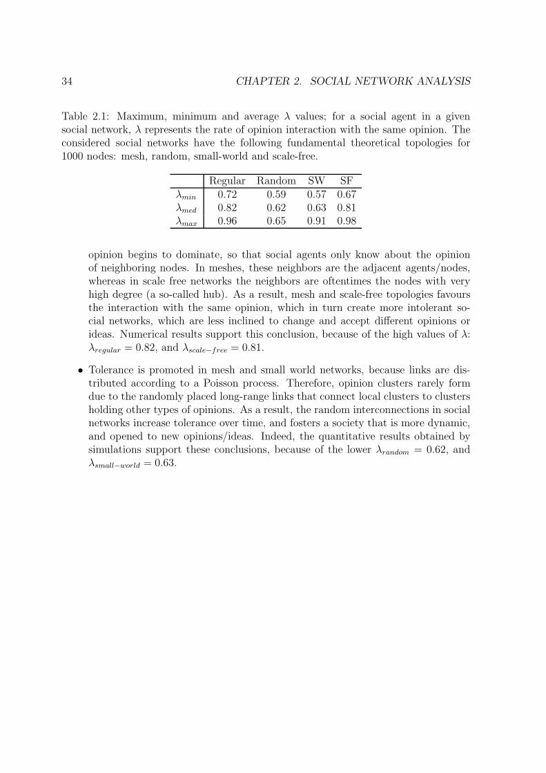
Table 2.1: Maximum, minimum and average λ values; for a social agent in a givensocial network, λ represents the rate of opinion interaction with the same opinion. Theconsidered social networks have the following fundamental theoretical topologies for1000 nodes: mesh, random, small-world and scale-free.
Regular Random SW SFλmin 0.72 0.59 0.57 0.67λmed 0.82 0.62 0.63 0.81λmax 0.96 0.65 0.91 0.98
opinion begins to dominate, so that social agents only know about the opinionof neighboring nodes. In meshes, these neighbors are the adjacent agents/nodes,whereas in scale free networks the neighbors are oftentimes the nodes with veryhigh degree (a so-called hub). As a result, mesh and scale-free topologies favoursthe interaction with the same opinion, which in turn create more intolerant so-cial networks, which are less inclined to change and accept different opinions orideas. Numerical results support this conclusion, because of the high values of λ:λregular = 0.82, and λscale−free = 0.81.
• Tolerance is promoted in mesh and small world networks, because links are dis-tributed according to a Poisson process. Therefore, opinion clusters rarely formdue to the randomly placed long-range links that connect local clusters to clustersholding other types of opinions. As a result, the random interconnections in socialnetworks increase tolerance over time, and fosters a society that is more dynamic,and opened to new opinions/ideas. Indeed, the quantitative results obtained bysimulations support these conclusions, because of the lower λrandom = 0.62, andλsmall−world = 0.63.

2.3. DISCUSSION AND CONCLUSIONS 35
2.3 Discussion and Conclusions
Our fundamental contribution to the field of social network interaction and opinionspread models consists of endowing social agent with more human-like traits like adapt-ability and inner predisposition to accept or to reject other people’s opinions andideas. As a result, our model is able to replicate real-world dynamic opinion phe-nomena, a feature that is not accessible to hitherto social interaction models such as[61][107][124][37][60][80][122]. Quantifying and modeling human action and inner moti-vation is a very difficult endeavor, therefore simulating and analyzing individual’s trust,faith, or tolerance states is still in its infancy. Our approach to this problem is to findinspiration in social psychology, in order to enhance the existing fixed-threshold socialinteraction models. In social psychology, individual tolerance is considered as an im-portant factor in the opinion dynamics of the entire society; au such, the concept ofegocentrism, is considered to be linked to individual’s internal emotional status [72].Our approach was to use this model due to the fact that egocentrism is a trait thatconnects to individual tolerance towards other opinions [204][185].
Moreover, in [191], we have analyzed our tolerance-based opinion interaction modelfrom a probabilistic standpoint, and correlate the findings with simulation results. Ourprobabilistic analysis explains opinion dynamics obtained by simulation or observedin real-world systems, especially when the society stabilizes, namely at t → ∞. Aspresented in figures 2.3 and 2.5, one of the most important results in our probabilisticassessment of the tolerance model is that tolerance is higher for the average social agentwith small ρ (i.e. the agent connects with a small number of NULL agents – socialagents that have no opinion).
Our probabilistic analysis in [191]assumes a 3-state Markov model (when we havejust one intermediary state between pure tolerance and pure intolerance) and a muchrealistic 4-state Markov model (with two intermediary states between pure toleranceand intolerance). Our assessment finds that the probability of tolerance decreases withλ (i.e. the rate of opinion interactions with the same opinion in the social network) inan almost linear fashion; this dependency becomes exponential for the 4-state model.These results suggest that real-life social interaction phenomena are non-linear; more-over, linear interpretations are mere overly simplistic approaches that are not reliableand cannot be used as prediction tools.
In [185] we show that by considering the tolerance-based opinion interaction model,we are able to reproduce dynamical features of opinion formation such as phase transi-tions and opinion formation phases. We also show that these non-linear dynamic opinionphenomena are influenced by underlying social network topology. In fact, we find thatthe topology has a stronger influence on opinion spread phenomena than, for instance,network size or stubborn agents placement and distribution. As such, mesh and scale-free networks correspond to conservative, oligarchic societies, whereas random and smallworld networks correspond to decentralized, democratic societies [185][191].

36 CHAPTER 2. SOCIAL NETWORK ANALYSIS

Chapter 3
Network Pharmacology andNetwork Medicine
3.1 Network Pharmacology
Over the last decade, the concept of drug repositioning (sometimes called drug repurpos-ing has been intensely researched and developed within the field of drug design. Drugrepositioning means uncovering new pharmaceutical properties and indications for al-ready existing drugs [171]. The motivation for the growing interest in drug repositioningstrategies is twofold. First, there are the notable advances in scientific fields such asbioinformatics, genomics, physics, complex networks, as well as technological fields suchas machine learning and database mining [123][57]. Second, there is a massive markeddemand for new drugs, although on the other hand the drug design process is slow andevermore expensive; as a result, entirely new approved pharmaceutical formulations arevery hard to get [65]. In this context, it seems like drug repositioning can be a moreaffordable alternative from both technical and economic standpoints [38][140][153][167].Indeed, a recent study has revealed that, as of now, we are already taking about 20%of the new drugs brought on the market as being drug repositionings [95]. Moreover,the available repositionings are made as part of personalized (or precision) medicineinitiatives [164].
Conventional drug repositioning is performed by using traditional-experimental ap-proaches stemming from biochemistry and genetics; however, many drug repositioningsare found by mere serendipity [28]. Nonetheless, our approach to this very importantpharmacological problem is powered by computational tools, which are linked to thecomplex network approach. Over the last decade, many such computational approacheswere developed, by taking advantage of the tremendous advances in big data gather-ing and machine learning; these computational solutions encompass a wide array ofissues from pharmacology and drug design, which include drug repositioning. As such,there are computational solutions for uncovering new drug interactions that were un-accounted during clinical trials [178]. Also, there are computational models used topredict the degree of drug safety during therapy [71][121]. For drug repositionings, com-putational approaches are processing and analyzing multiple comprehensive databasessuch as drug, genomic, transcriptomic, and phenotypic databases [123]. However, the
37
38 CHAPTER 3. NETWORK PHARMACOLOGY AND NETWORK MEDICINE
results of all these computational methods are mere predictionss, which will have to bevalidated by traditional in vivo and in vitro) experimental methods [123].
Many computational methods for drug repurposings are based on recent advancesin the new science of complex networks as well as on the fact that we have access toan evermore increasing volume of data about medication (including approved, investi-gational and experimental drugs). Some of the most available and easy-to-get data onmedication consists of drug-drug interactions, namely data about the way drug effectsinteract when taken together according to some therapeutic schema. Consequently, oneof the most important tool in translational, systems and computational pharmacology isbased on drug-drug interactomes (DDI); DDIs are complex network with nodes/verticesrepresenting pharmaceutical substances (i.e. drugs) and links representing drug inter-actions (e.g. common mediation by a some enzyme, or synergistic effects). There aremany advantages in using drug interactomes (DDI) for analysis, but the most importantapplications are:
• Predicting new potential interactions [178][105]; based on this principle, manysoftware products were developed in order to issue drug interaction alerts [177].
• Avoiding certain types of drug-drug interactions even from the drug design stage[47][165].
• Exploring the links between pharmaceutical properties and drug interactions; pre-viously, this idea was mostly applied for predicting new drug-drug interactionswhen we have verified information about confirmed interactions [156][111].
Recent developments aim at using interaction information from DDIs to uncover newdrug effects and properties, thus paving the way for drug repositioning [125]. As such,[210] processes a DDI with the Markov Clustering Algorithm, in order to predict newdrug functions. Another research takes information about drug side effects from socialmedia (Twitter), in order to build a corresponding DDI and then predict possible drugrepurposings [148].
3.1.1 Drug-drug interaction network analysis
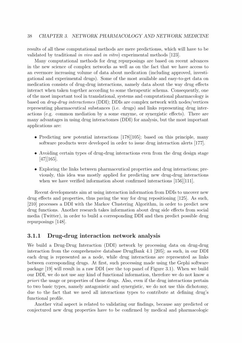
We build a Drug-Drug Interaction (DDI) network by processing data on drug-druginteraction from the comprehensive database DrugBank 4.1 [205]; as such, in our DDIeach drug is represented as a node, while drug interactions are represented as linksbetween corresponding drugs. At first, such processing made using the Gephi softwarepackage [19] will result in a raw DDI (see the top panel of Figure 3.1). When we buildour DDI, we do not use any kind of functional information, therefore we do not know apriori the usage or properties of these drugs. Also, even if the drug interactions pertainto two basic types, namely antagonistic and synergistic, we do not use this dichotomy,due to the fact that we need all interactions types to contribute at defining drug’sfunctional profile.
Another vital aspect is related to validating our findings, because any predicted orconjectured new drug properties have to be confirmed by medical and pharmacologic

3.1. NETWORK PHARMACOLOGY 39
Figure 3.1: Drug-drug interactome (DDI) computer processing methodology for clus-tering drugs based on modularity classes and force-directed topological clustering. Theclustering result is correlated with several pharmacological properties, thus creatingincentives for predicting drug repositionings.

40 CHAPTER 3. NETWORK PHARMACOLOGY AND NETWORK MEDICINE
tools (i.e. in vivo and in vitro). Therefore, we find the following validation proce-dure as convenient. We use the older 4.1 DrugBank version for building and analyzingour DDI, in order to spare the newer DrugBank 4.3 for validating the predicted newpharmacological properties.
In order to cluster the drugs in the DDI we use the methodology from Figure 3.1: weclassify network nodes to modularity classes that are depicted with distinct colors [147]and, at the same time, by using the force-directed layout algorithm Force Atlas 2 [108]we generate well-defined topological communities which also act ass clusters. The visualresult is what we call Community Based Drug-Drug Interaction Network (CBDDIN)from Figure 3.2.
The novelty of our methodology [190] is that it uses for the first time in the field ofdrug interactomes the network analysis tools which are conventionally deployed only forsocial networks. Such an approach is further motivated by the fact that there is a goodsimilarity in terms of network parameters between our DDI and a typical social network:low average path length of L = 2.978 given the network diameter Dmt7, a relativelyhigh clustering coefficient C = 0.2, high average degree < k >= 20.031, typical valuesfor modularity Mod = 0.452 and density Dst = 0.017.
In terms of network centrality metrics, our DDI is characterized by the distributionsfrom Figure 3.3: power-law degree, betweenness and eigenvector distributions, normalcloseness distribution. In qualitative terms, these distribution types indicate a scale-freenetwork.
In DrugBank Version 4.1 [205] there is a total of 7739 drug entries (including, be-sides approved drugs, experimental and investigational drugs). As some of these drugentries have no information about interactions, we remove them because they cannotbe connected to the DDI; after the removal process, 1141 drugs will remain. However,additional data is required to verify and validate our predictions; to this end, we cross-check with functional properties that are listed in other databases such as Drugs.com,RxList, and DrugBank 4.3. Also, a good amount of validation is performed by simplysearching scientific literature from online article databases.
3.1.2 Interpreting network centralities
Our CBDDIN is shaped by the collection of drug-drug interactions relationships, hencedrugs that have the highest centralities (e.g. degree, betweenness) are the most pre-disposed to other drug-drug interactions. As such, we can scorecard the interactionpotential of drugs from CBDDIN; table 3.1 introduces only the top 10 drugs in termsof degree, betweenness, closeness, page rank, and eigenvector.
Description of drug clusters
Topological clusters from Figure 3.2 are generated with the Force Atlas 2 [108] lay-out algorithm, while the modularity clusters (which are correspondingly labeled withdistinct colors) are automatically generated in Gephi [93]. We identify an underly-ing, generally common property for all topological communities; this labeling processis made by individualizing a pharmacological property which best describe the biggest

3.1. NETWORK PHARMACOLOGY 41
Figure 3.2: Our visual DDI clustering, resulted as the Community-Based Drug-DrugInteraction Network (CBDDIN). Both modularity classes (labeled with colors) and force-directed (Force Atlas 2) clusterings are generated in Gephi, by processing the drug-druginteraction data taken from DrugBank 4.1 (consisting of 1141 drugs and 11688 drug-druginteractions).
Table 3.1: Top 10 hierarchies of drugs from Community-based drug-drug interaction net-work (CBDDIN) in terms of degree, betweenness, closeness, page rank, and eigenvectorvalues.
Degree Betweenness Closeness Page rank EigenvectorDrug Value Drug Value Drug Value Drug Value Drug Value
1. Voriconazole 250 Triprolidine 47.570 Voriconazole 2.077 Triprolidine 0.009 Voriconazole 12. Triprolidine 198 Trastuzumab 37.522 Ketoconazole 2.121 Voriconazole 0.009 Telithromycin 0.8513. Telithromycin 198 Treprostinil 37.168 Phenytoin 2.128 Treprostinil 0.008 Trimipramine 0.8454. Warfarin 181 Warfarin 34.129 Cyclosporine 2.141 Warfarin 0.008 Rifampin 0.6835. Trimipramine 174 Cyclosporine 33.217 Telithromycin 2.142 Trastuzumab 0.007 Tramadol 0.6826. Ketoconazole 161 Tacrolimus 30.491 Tacrolimus 2.155 Telithromycin 0.007 Tacrolimus 0.6807. Rifampin 157 Tacrine 27.734 Warfarin 2.168 Cyclosporine 0.006 Trazodone 0.6568. Cyclosporine 150 Phenytoin 22.018 Rifampin 2.171 Ketoconazole 0.006 Ketoconazole 0.6569. Phenytoin 147 Ketoconazole 21.598 Trimipramine 2.180 Tacrine 0.006 Quinidine 0.62310. Tacrolimus 147 Rifampin 21.288 Fosphenytoin 2.184 Rifampin 0.006 Clarithromycin 0.609

42 CHAPTER 3. NETWORK PHARMACOLOGY AND NETWORK MEDICINE
Figure 3.3: Centrality distributions for our CBDDIN: A) degree, B) betweenness, C)closeness, and D) eigenvector. We also provide the slope α and cutoff point Xmin valuesfor all power-law distributions. For the normal distribution of closeness, we provide the
best Gaussian fit as f (x) = 1.654 + 9.768 exp(
−(x−2.896)2
2·0.362
)
.
majority of nodes/drugs within each cluster. For some clusters, the label targets anorgan or system, for others a medical indication, or a well-defined chemical structure.Nonetheless, we do not put functional limits to our labeling process, because we needto obtain the specific property which better identifies the biggest number of drugs fromeach cluster/community.
The labeling of modularity classes from Table 3.2 is very consistent, as the tagscharacterize very well almost all drugs in CBDDIN. This result is confirmation of pre-vious results which indicate modularity as an outstanding predictor of functionality inbiological systems [144]. Indeed, because CBDDIN is shaped by the distribution of linkdensity, in our approach modularity is very well connected with the concept of druginteractions.
As presented in Figure 3.2, we identify and label accordingly a number of 9 topolog-ical clusters; the accuracy of Figure 3.2’s labeling is given, in Table 3.3 as confirmationpercentages. Each community contains nodes/drugs for which their assigned modularityclass actually confirms the topological cluster label. The percentage of topological clus-ter label confirmation with modularity classes is given in the column ”Conf. by mod.[%]”. Also, by cross validating with state of the art literature in the fields of pharma-cology and biology and by confronting with other databases (Drugs.com [211], RxList[212], DrugBank 4.3 [205], we further explain topological community labels for lots ofother drugs. The overall result of cross-validating and label confirmation is presentedin the 5th column of Table 3.3.

3.1. NETWORK PHARMACOLOGY 43
Table 3.2: Interpretation and labeling og CBDDIN modularity classes, according tomodularity clustering algorithm. The allocated labels correspond to pharmacologicalproperties (see column ”Modularity class interpretation”). We also indicate the numberof drugs in each modularity class, as well as the percentage of drugs that correspond tothe allocated label (columns ”No. of drugs” and ”Consistency [%]”).
Modularity class (color) Code Modularity class interpretation No. of drugs Consistency [%]Dark blue DB Central and peripheral nervous system acting drugs 232 96Velvet maroon VM Substrates, inhibitors and inducers of specific CYP en-
zymes210 91
Green G Drugs that interfere in different phases of hemostasis, an-ticonvulsant and epileptogenic drugs
191 85
Magenta M Drugs acting on sympathetic nervous system 166 93Light blue LB Drugs targeting cancer, auto-immune disorders (i.e.
rheumatoid arthritis), and musculoskeletal system156 88
Golden brown GB Drugs interfering with platelet activity and plasma potas-sium levels
155 92
Purple P Bi-and trivalent cations, chelating agents 31 100
Table 3.3: CBDDIN labels for each of the nine topological clusters. The 2nd columnpresent the modularity classes (identified with colors) which confirm the topologicalcluster tag. The 3rd column gives the total number of drugs in each topological cluster,which is then broken to the following categories: correctly described by the assignedmodularity class (Conf. by mod.), explained by properties listed in drug databases andstate of the art literature (Expl. by propr.), and not explained yet (Not expl.)
Comm. Colors No. Conf. by mod.[%]
Expl. bypropr. [%]
Not expl.[%]
I LB, VM 80 77 19 4II VM, GB, G, DB, LB,
M271 80 8 12
III DB, M, LB, GB 307 84 12 4IV M, GB, G, DB 81 51 22 27V GB 54 33 63 4VI GB, G, LB, M, P 125 35 38 27VII LB 58 26 31 43VIII P, G, LB, GB 69 56 9 35IX G, LB 96 30 57 13
1141 63 22 15

44 CHAPTER 3. NETWORK PHARMACOLOGY AND NETWORK MEDICINE
Overall, the most important result is that our methodology can extract pharmaco-logical properties only from drug-drug interaction data. As such, 63% of the assigneddrug property labels are in agreement with the drug properties already listed in Drug-Bank 4.1; additionally, 22% of included drugs are not listed with the assigned propertyin DrugBank 4.1 but are confirmed as correctly labeled, by an extensive cross-checkingprocess which employs literature survey and other public drug databases. As a result,the remaining 15% of the drugs seem to be out of place according to their respectivetopological cluster labeling; such situations represent opportunities for predicting drugrepositionings. Indeed, repositioning assumptions can be made by simply analyzing thecases which seem as not compliant with topological or modularity cluster labels. Welisted all seemingly non-compliant drug cases in column Not expl. [%] (not explained)from Table 3.3. Consequently, we predict that drugs listed as not explained can berepurposed in accordance with a pharmacological property that is given by either theirmodularity or their topological cluster labels.
Apart from the most obvious approach based on label non-compliance, there is an-other valid repurposing strategy, namely analyzing drugs which lie at the frontiers be-tween two or mode topological clusters; the assumption is that such borderline situationsmay indicate multiple pharmacological properties pertaining to the neighboring clusters.
According to our contributions [190], a short functional, pharmacological descriptionof the topological clusters generated with our methodology is given below:Cluster I Antineoplastic agents, immuno-stimulants and immunosuppressants.Cluster II Substrates, inhibitors and inducers of specific cytochrome P450 enzymeswhich mostly have a CYP-related activity.Cluster III Drugs that affect the metabolism of neurotransmitters, thus incurring cen-tral and peripheral nervous effects.Cluster IV Drugs which act on alpha- and beta- adrenoreceptors, which mostly includethe cases of drugs related to sympathetic nervous system (SNS) effects [104][117][196][112]).Cluster VMost drugs from this cluster consist of renin-angiotensin system acting drugsand diuretics, but we can also find some platelet aggregation inhibitors [114].Cluster VI Drugs which interfere with different phases of hemostasis.Cluster VII Drugs that have neuromuscular-blocking activity, from both pharmaco-dynamic and pharmacotoxicologic perspectives [152][53].Cluster VIII This cluster mostly consist of bivalent and trivalent metal cations, aswell as of their corresponding chelators [141][205][182][135].Cluster IX Drugs employed for treating various types of epilepsy and seizure, as wellas epileptogenic drugs [175][49].
Examples of finding new properties
To illustrate how our network-based is able to predict multiple pharmacological proper-ties and already known repositionings, using only drug-drug interaction data, we presentthe cases of Zafirlukast and Thalidomide:
• Zafirlukast is a drug used in asthma therapy; its positioning in Cluster II (Fig-ure 3.4A) is motivated by the fact that it is CYP3A4 substrate and inhibitor[205][212]. However, as opposed to most other drugs from Cluster II, zafirlukast is

3.1. NETWORK PHARMACOLOGY 45
Figure 3.4: CBDDIN details that present: A) the position of Zafirlukast in Cluster II;B) the position of Thalidomide in Cluster I.
pertains to the golden brown (GB) modularity class; this property is confirmed byzafirlukast’s platelet activity [116]. Indeed, this example shows how our dual clus-tering methodology (modularity class plus energy-model layout) is able to recovermultiple properties.
• Thalidomide is a recent example of drug repositioning. Initially, thalidomide wasdesigned for thwarting pregnant women’s morning sickness, but it was later with-drawn because of its adverse effects on embryos. However, as of today thalido-mide is employed for treating immunological and inflammatory disorders [180].This newly found property is also predicted by our method, as presented in Fig-ure 3.4B: thalidomide pertains to the light blue LB modularity class (Anti-cancerdrugs) and is placed within Cluster I (Immune system related drugs).
3.1.3 Results Interpretation
The fact that our drug-drug interaction network clustering methodology generates 9well-defined pharmacological characteristics (as presented in Figure 3.2) may suggestthat the 9 properties have essential roles in drug-drug interaction mechanisms. Assuch, the fact that 9 pharmacological properties have a stronger influence on drug-druginteractions is in itself a significant contribution.
In terms of accuracy, our prediction of pharmacologic properties is validated for 85%of the drugs with functional information taken from DrugBank 4.1., from other drugdatabases, and from literature surveys. Hence, motivated by this high prediction accu-racy, we argue that it is extremely likely that – in the future – the predicted propertieswill also be confirmed for the remaining 15%.
In our CBDDIN there are many possible repositionings. For instance, the drugchlorzoxazone is predicted by our method as haing immunological properties, as it ispositioned in Cluster I. Also, cefalosporin antibiotics such as cefalotin, cefamandole,or cefixime, are predicted as acting on the immune system or neuromuscular junction,because they pertain to Cluster VII. Moreover, predicting new properties may lead to

46 CHAPTER 3. NETWORK PHARMACOLOGY AND NETWORK MEDICINE
predicting new interactions. Indeed, drugs bevacizumab and lorazepam are placed inCluster II, so that can be predicted as interfering with CYP enzymes. Nonetheless, com-putational models can only make useful repositioning hints, which may be subsequentlyconfirmed by in vivo and in vitro biomedical tools. To this end, we indicate that thesedrugs be further investigated to confirm new repositionings or interactions.
From a fundamental perspective, drug-drug interactions actually express the waythat drug behaviors interfere, constructively or destructively. Consequently, it can besaid that our network clustering repositioning methodology is acting at behavioral level.Such an approach is contrasting with most hitherto network-based repositioning strate-gies, which rely on chemical structure similarity relationships or drug-target relation-ships. We consider our work as a strong argument for the multi-level network approachto drug repurposing, an approach that integrates the behavioral and structural perspec-tives [209]. In this context, we identify DARPA’s Big Mechanism project [43] as anappropriate platform for multi-level integration.
Our methodology from Figure 3.1 can also be used for clustering patients in medicaldatabases, for instance in cardiovascular disorders [176], sleep apnea syndrome [186], ordefining endophenotypes [92]. These studies prove that disease risk factors do not as-sociate at random, they rater converge towards well-defining patient phenotypes, whichin turn provide valuable information for precision medicine approaches.
3.2 Network Medicine
Obstructive Sleep Apnea Syndrome (OSAS) is a serious clinical disorder caused by ab-normal breathing pauses that occur during sleep; this results in sleep fragmentation andexcessive daytime somnolence [170][84][120]. There are studies reporting the epidemicincidence of OSAS, with worrying increasing rates over the last 20 years [208][157][155].If not properly diagnosed and treated, OSAS increases the morbidity and perioperativerisks [132][131][159][193][161].
Apnea severity is indicated by the Apnea-Hypopnea Index AHI; this represents thenumber of breathing pauses of at least 10 seconds, recorded over one hour of sleep. Assuch, any patient can be classified in one of the following AHI categories: normal orlow-risk apnea (L) for AHI < 5, mild sleep apnea (Mi) for 5 ≤ AHI < 15, moderatesleep apnea (Mo) for 15 ≤ AHI < 30, and severe sleep apnea (Se) when AHI ≥ 30.
Usually, polysomnography (PSG) is used as the reference method (i.e. gold standard)of OSAS diagnosis, which is based on measuring AHI. However, PSG is expensive,time-consuming, and generally not adequate for population screening. [170][163]. SinceOSAS has a significant prevalence and the PSG-based exhaustive investigation is notfeasible when screening a large population, OSAS predictors are preferred for monitoring[192][184].
In current practice, there are three major predictive models based on questionnaires,namely Berlin, STOP, and STOP-BANG [142][169][81][50][51]. Published studies in-dicate STOP-BANG as the best available predictive score, due to its high sensitivity:83.6% for AHI > 5, 92.9% for AHI > 15, and 100% for AHI > 30. However, STOP-BANG has a low specificity (56.4% for AHI > 5, 43% for AHI > 15, and 37% for
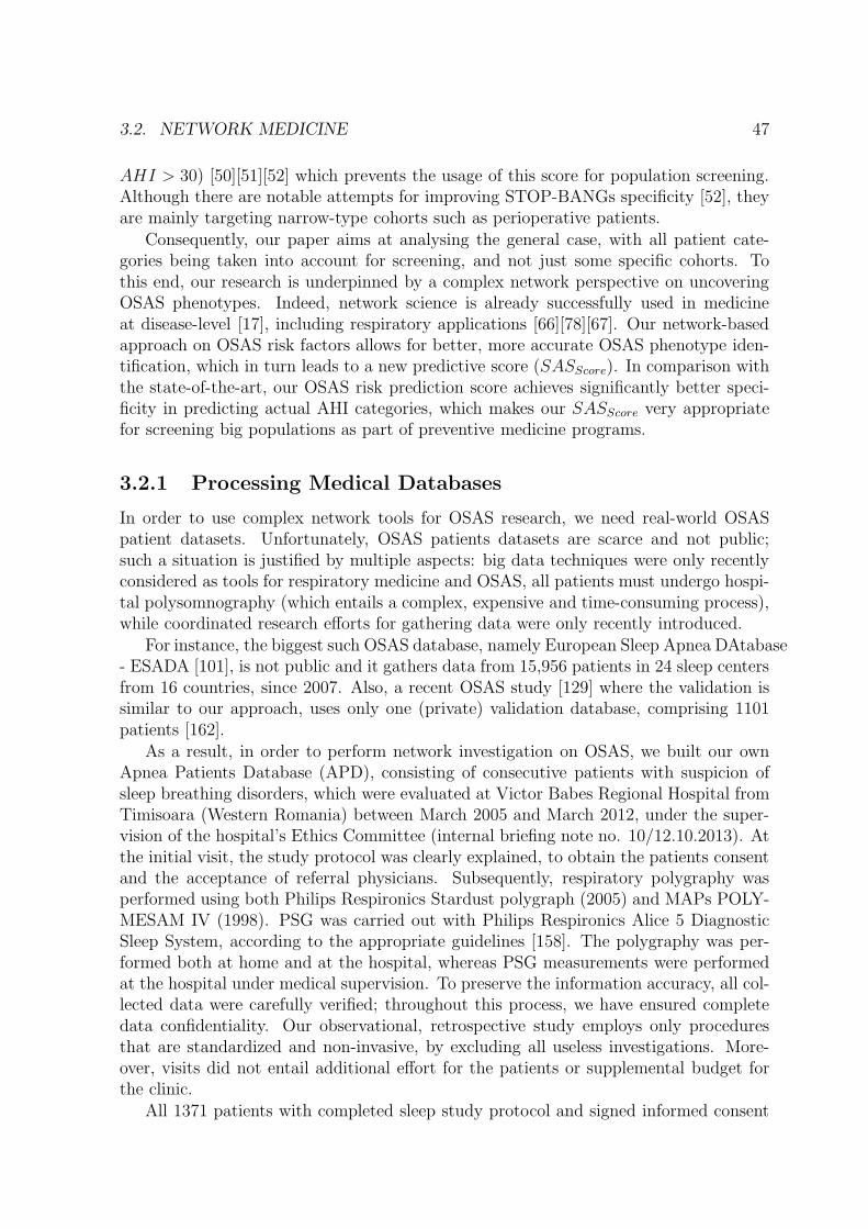
3.2. NETWORK MEDICINE 47
AHI > 30) [50][51][52] which prevents the usage of this score for population screening.Although there are notable attempts for improving STOP-BANGs specificity [52], theyare mainly targeting narrow-type cohorts such as perioperative patients.
Consequently, our paper aims at analysing the general case, with all patient cate-gories being taken into account for screening, and not just some specific cohorts. Tothis end, our research is underpinned by a complex network perspective on uncoveringOSAS phenotypes. Indeed, network science is already successfully used in medicineat disease-level [17], including respiratory applications [66][78][67]. Our network-basedapproach on OSAS risk factors allows for better, more accurate OSAS phenotype iden-tification, which in turn leads to a new predictive score (SASScore). In comparison withthe state-of-the-art, our OSAS risk prediction score achieves significantly better speci-ficity in predicting actual AHI categories, which makes our SASScore very appropriatefor screening big populations as part of preventive medicine programs.
3.2.1 Processing Medical Databases
In order to use complex network tools for OSAS research, we need real-world OSASpatient datasets. Unfortunately, OSAS patients datasets are scarce and not public;such a situation is justified by multiple aspects: big data techniques were only recentlyconsidered as tools for respiratory medicine and OSAS, all patients must undergo hospi-tal polysomnography (which entails a complex, expensive and time-consuming process),while coordinated research efforts for gathering data were only recently introduced.
For instance, the biggest such OSAS database, namely European Sleep Apnea DAtabase- ESADA [101], is not public and it gathers data from 15,956 patients in 24 sleep centersfrom 16 countries, since 2007. Also, a recent OSAS study [129] where the validation issimilar to our approach, uses only one (private) validation database, comprising 1101patients [162].
As a result, in order to perform network investigation on OSAS, we built our ownApnea Patients Database (APD), consisting of consecutive patients with suspicion ofsleep breathing disorders, which were evaluated at Victor Babes Regional Hospital fromTimisoara (Western Romania) between March 2005 and March 2012, under the super-vision of the hospital’s Ethics Committee (internal briefing note no. 10/12.10.2013). Atthe initial visit, the study protocol was clearly explained, to obtain the patients consentand the acceptance of referral physicians. Subsequently, respiratory polygraphy wasperformed using both Philips Respironics Stardust polygraph (2005) and MAPs POLY-MESAM IV (1998). PSG was carried out with Philips Respironics Alice 5 DiagnosticSleep System, according to the appropriate guidelines [158]. The polygraphy was per-formed both at home and at the hospital, whereas PSG measurements were performedat the hospital under medical supervision. To preserve the information accuracy, all col-lected data were carefully verified; throughout this process, we have ensured completedata confidentiality. Our observational, retrospective study employs only proceduresthat are standardized and non-invasive, by excluding all useless investigations. More-over, visits did not entail additional effort for the patients or supplemental budget forthe clinic.
All 1371 patients with completed sleep study protocol and signed informed consent

48 CHAPTER 3. NETWORK PHARMACOLOGY AND NETWORK MEDICINE
are included in the APD, each with corresponding 108 breathing parameters and an-thropometric measurements. The APD distribution of measured AHI is presented inFigure 3.5.
Figure 3.5: Log-linear histogram representing the number of patients with a certainApnea-Hypopnea Index (AHI) value, along with the corresponding distribution fit.The best fit is the exponential function f(x) = 27.453 · e−0.025x.
In order to verify if there is any difference between apnea and non-apnea populationsin terms of how risk factors associate and converge, we built a 611 people non-OSASdatabase NAD (using the same procedure as for the APD). Also, to evaluate the pre-diction score derived from our study, we gathered a distinct test database TD (fall of2013) consisting of 231 patients, by following the same procedure. Figure 3.6 presentsthe distinct roles of our 3 databases, as well as the relationship between them.
Analysis of APD and TD
As patients within TD are used to validate our OSAS prediction with SASScore, whichwas obtained by processing patients from APD, we analyse if the distribution of param-eters in TD is not too close to the corresponding distributions in APD. Such an investi-gation is required considering that, although data for the two databases were gatheredover distinct periods of time, all measurements were performed in a given geographicalregion, with subjects that mostly pertain to Caucasian anthropological characteristics.
To this end, we present the distributions of the most relevant parameters in ourresearch (Age A, Body Mass Index BMI, Neck Circumference NC, High Blood PressureHBP , and Epworth Sleepiness Score ESS), within the validation population (TD) andthe apnea patients database (APD) in Table 3.4, under the form of measured averagesand their corresponding standard deviations, as well as Gini coefficients. We rely onGini coefficients for a quantitative measure of data dispersion.
We also provide a visual comparison of AHI and relevant risk factor parametersdistributions in APD and TD (see Figure 3.7). All these results show that, given thatdatabases contain subjects from a well-delimited geographical area and were randomly

3.2. NETWORK MEDICINE 49
Figure 3.6: Description of databases used in our research. The main Apnea PatientsDatabase (APD), comprising 1371 consecutive patients which arrive at the hospital withsuspicion of OSAS between 2005 and 2012, is used to build patient phenotypes and torender the SASScore. The distinct Test Database (TD), comprising 231 consecutivepatients which arrive at the hospital with suspicion of OSAS in 2013, is used to verifythe sensitivity and specificity of predicting patient’s AHI and OSAS categories. TheNon-OSAS patients Database (NAD) uses consecutive assessed people which are notdiagnosed with OSAS during the spring 2015 – summer 2016 period, in order to test forcluster consistency (i.e. compare how risk factors converge in clusters for OSAS patientsin comparison with people without OSAS).
gathered, the main parameter distributions are somehow similar - mostly normally dis-tributed. However, Gini coefficients (especially for A, BMI and ESS) indicate animportant difference between APD and TD distributions. Moreover, Figure 3.7 shows asignificantly different AHI histogram for TD in comparison with APD. As such, in APDthere are many patients with AHI > 120, whereas in TD there is none such patient.Also, in APD, the largest number of patients associated to an AHI value correspond toAHI values < 20; in contrast, in TD, the largest number of patients with a given AHIvalue correspond to AHI values around 40.
Building the patient network
An unweighted network is a graph (V,E), which consists of a set of vertices (or nodes)V and a set of edges (or links) E that represent connections [v, w] ∈ E between certainpairs of vertices v, w ∈ V . We build the unweighted Apnea Patients Network (APN), byassigning vertices and edges: each node corresponds to a distinct patient in our OSASpatients database APD, while an edge (link) is created between two vertices if there is arisk factor compatibility between the patients represented by the two vertices (nodes).
The risk factor compatibility is a binary function fRFC ∈ {0, 1} (0 means incom-patibility and 1 means compatibility) based on six parameters with high relevance forOSAS: age, gender, BMI, neck circumference, blood pressure (systolic and diastolic),and Epworth Sleepiness Score. We build our APN by considering that fRFC = 1 if atleast 4 out of 6 parameters are identical; otherwise fRFC = 0.

50 CHAPTER 3. NETWORK PHARMACOLOGY AND NETWORK MEDICINE
Figure 3.7: AHI distributions in APD (panels A, C, E, G, I) and TD (panels B, D, F,H, J), as well as the normal distributions of BMI, Age A, Neck Circumference NC andESS, for patients in both APD and TD.

3.2. NETWORK MEDICINE 51
ParameterAPD TD
Average Gini Average Gini
AHI 40.04± 27.83 0.388 44.39± 26.13 0.334BMI 33.01± 7.94 0.576 32.62± 7.41 0.468A (yrs.) 51.73± 12.44 0.539 52.01± 13.61 0.397NC (cm.) 42.01± 9.94 0.51 42.64± 5.12 0.482HBP 67.47% N/A 64.93% N/AESS 10.63± 5.38 0.362 11.38± 5.19 0.422
Table 3.4: AHI and relevant risk factor parameters distribution in the Apnea PatientsDatabase (APD) and Test Database (TD), given as average values plus standard devia-tion, as well as Gini coefficients. We only considered boolean values for the High BloodPressure (i.e. if the patient has high blood pressure or not); in this case, we providedthe percentages of people with high blood pressure.
The six parameters are selected from the pool of all relevant risk factors (all measuredparameters can be found in the supplementary file Apnea-Patients-Database-(APD)-and-Test-Database-(TD).xlsx), because they can be measured easily and objectively;such objective measurements can be performed anywhere, and are widely accepted in themedical literature [120]. In contrast, other scores consider snoring and witnessed apneaepisodes as factors, but these are parameters which cannot be observed or measuredobjectively.
The reason for adopting the 4-out-of-6 criterion is that it assures the right amountof link density in the APN, meaning that there are enough links so that the APN isconnected, but not too many links so that communities (i.e. clusters) can be renderedwith energy model layouts [147]. As Figure 3.8 shows that the 4 out of 6 link filteringrepresents the best alternative, we use this criterion to build the APN. To the best ofour knowledge, this link filtering procedure is original and hasnt been used before insuch network-based approaches.
APN clustering
We clustered the APN, by using a dual clustering methodology: energy-model layoutsplus modularity classes, similar to the approach from [190]. Energy-models are forcedirected network layout algorithms, namely visual tools that assign certain positions inthe Euclidian space to both nodes and edges [147]. To this end, we used the Force Atlas 2algorithm [108] as network layout; this new layout is very effective in clustering varioustypes of complex networks, as it is based on previous theoretical foundation of forcedirected attraction-repulsion algorithms [87][146]. Indeed, Force Atlas 2 is clusteringcomplex networks by producing well-defined topological clusters. The overview of theentire clustering process, including testing cluster convergence with non-OSAS controlpatients and validation of SASScore, is presented in Figure 3.9. In addition to the layoutalgorithm, we used modularity-based network clustering [93], a method that was provento be effective in network medicine [66][78].
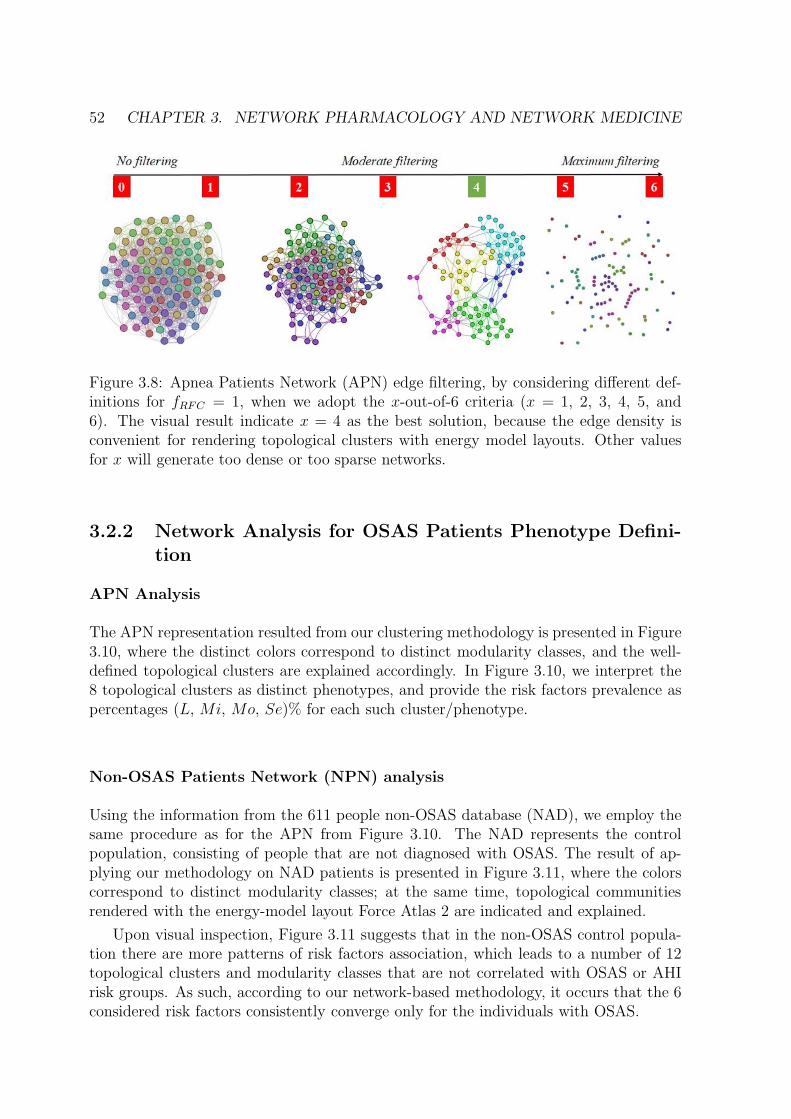
52 CHAPTER 3. NETWORK PHARMACOLOGY AND NETWORK MEDICINE
Figure 3.8: Apnea Patients Network (APN) edge filtering, by considering different def-initions for fRFC = 1, when we adopt the x-out-of-6 criteria (x = 1, 2, 3, 4, 5, and6). The visual result indicate x = 4 as the best solution, because the edge density isconvenient for rendering topological clusters with energy model layouts. Other valuesfor x will generate too dense or too sparse networks.
3.2.2 Network Analysis for OSAS Patients Phenotype Defini-tion
APN Analysis
The APN representation resulted from our clustering methodology is presented in Figure3.10, where the distinct colors correspond to distinct modularity classes, and the well-defined topological clusters are explained accordingly. In Figure 3.10, we interpret the8 topological clusters as distinct phenotypes, and provide the risk factors prevalence aspercentages (L, Mi, Mo, Se)% for each such cluster/phenotype.
Non-OSAS Patients Network (NPN) analysis
Using the information from the 611 people non-OSAS database (NAD), we employ thesame procedure as for the APN from Figure 3.10. The NAD represents the controlpopulation, consisting of people that are not diagnosed with OSAS. The result of ap-plying our methodology on NAD patients is presented in Figure 3.11, where the colorscorrespond to distinct modularity classes; at the same time, topological communitiesrendered with the energy-model layout Force Atlas 2 are indicated and explained.
Upon visual inspection, Figure 3.11 suggests that in the non-OSAS control popula-tion there are more patterns of risk factors association, which leads to a number of 12topological clusters and modularity classes that are not correlated with OSAS or AHIrisk groups. As such, according to our network-based methodology, it occurs that the 6considered risk factors consistently converge only for the individuals with OSAS.

3.2. NETWORK MEDICINE 53
Figure 3.9: Overview of the proposed dual clustering methodology (modularity classesrepresented with distinct colors and topological clusters emerged from running the forcedirected layout Force Atlas 2), along with testing cluster formation against non-OSAScontrol patients (i.e. showing that risk factors converge differently for OSAS and non-OSAS patients), cluster consistency and SASScore validation.
Description of Phenotypes
In order to have a clear characterization of our rendered phenotypes, we are trackingthe OSAS comorbidities (as recorded in the APD) within the APN. To this end, weconsider the comorbidity types: cardiovascular (e.g. hypertension or stroke), nutritional(e.g. obesity or diabetes), and respiratory-related (e.g. COPD or asthma). Figure3.12 presents the highlighted comorbidities within the APN, by using distinct colorsfor comorbidity types that appear individually, as well as for comorbidity type overlaps(cardiovascular + nutritional, cardiovascular + respiratory, nutritional + respiratory,cardiovascular + nutritional + respiratory), and patients without known comorbidities.

54 CHAPTER 3. NETWORK PHARMACOLOGY AND NETWORK MEDICINE
Figure 3.10: Apnea Patients Network (APN) obtained with data from the Apnea Pa-tients Database (APD), according to the risk factor compatibility relationship, using ourdual network clustering methodology (i.e. modularity classes and energy-model layouts).The assigned colors correspond to modularity classes, and the 8 topological clusters areindicated. For each topological cluster, statistics are provided in red (as percentages)for all AHI risk groups: low, mild, moderate, and severe, using the format (L, Mi, Mo,Se)% (e.g. in Cluster 2 the patients are distributed on risk groups as follows: 9% L,15% Mi, 19% Mo, 57% Se). The risk group classification is made with AHI valuesthat are obtained by actually performing polysomnography (PSG) and polygraphy.

3.2. NETWORK MEDICINE 55
Figure 3.11: Non-OSAS Patients Network (NPN), obtained with data from the non-OSAS database (NAD) control population database. The colors correspond to 12 mod-ularity classes. Also, the energy-model layout Force Atlas 2 generates 12 topologicalclusters, which are described in terms of risk factors and their correspondence with themodularity classes.
In light of comorbidity and AHI risk groups statistics provided in Table 3.5 for eachcluster resulted from our network analysis (as illustrated in Figures 3.10 and 3.12), wecharacterize the phenotypes as follows:
• Phenotype 1: Mostly patients within the Se AHI risk group, which are generallyobese males with thick neck, high blood pressure, sleepiness, and age between 40and 60 years. For a large majority of these patients, all comorbidity types overlap.
• Phenotype 2: The large majority of these patients have Mo and Se apnea forms;they are obese females with thick neck, high blood pressure, sleepiness, age between40 and 60 years. In this phenotype there are no patients with only respiratorycomorbidities and only few of them have single nutritional comorbidities.
• Phenotype 3: The patients have mostly Mo and Se apnea, but there are lessSe forms in comparison with other phenotypes; they are obese females with thinneck, high blood pressure, no sleepiness, and age between 40 and 60 years. Thisphenotype does not contain patients with only respiratory comorbidities.
• Phenotype 4: Mostly Se patients; however, there is a significant number of Moindividuals, which are generally obese males with thick neck, high blood pressure,

56 CHAPTER 3. NETWORK PHARMACOLOGY AND NETWORK MEDICINE
sleepiness, and over 60 years. In this phenotype only a few patients have the singlerespiratory comorbidities type.
• Phenotype 5: Mostly Se, Mo, and Mi patients, which are obese young maleswith thick neck, high blood pressure, no sleepiness, and age between 20 and 40. Inthis phenotype, almost all patients have nutritional comorbidities or comorbidityoverlaps that include the nutritional type.
• Phenotype 6: Consists of mostly Mo and Se apnea; the patients within thisphenotype are generally obese males with thick neck, no high blood pressure, nosleepiness, and middle aged (40-60 years old). Their comorbidities are mostlynutritional-related (either single nutritional comorbidity or an association of co-morbidities that contains the nutritional type).
• Phenotype 7: Patients with mostly Mo and Se apnea, but with less Se forms incomparison with other phenotypes; this phenotypes patients are generally malesof all ages with thin neck, no high blood pressure, and no sleepiness. The majorityof these patients have no comorbidities; however, those who have a comorbiditytend to have respiratory-related problems.
• Phenotype 8: Patients mostly within Se, Mo, and Mi AHI risk groups; theyare males from all age groups with thin neck, no sleepiness, but with high bloodpressure. These patients tend to have a single cardiovascular comorbidity type oran association of comorbidities that include the cardiovascular type.

3.2. NETWORK MEDICINE 57
Figure 3.12: The Apnea Patients Network (APN), with highlighted individual comor-bidities and associations of comorbidities. The red nodes correspond to patients thathave only cardiovascular comorbidities (C in panel A), the yellow nodes to only nutrition-related (N in panel B), and blue nodes represent OSAS patients with only respiratorycomorbidities (R in panel C). Patients with overlapping comorbidity types are rep-resented within the APN as follows: orange nodes correspond to cardiovascular plusnutritional comorbidities (C + N in panel D), purple nodes to cardiovascular plus res-piratory comorbidities (C + R in panel E), green nodes to nutritional plus respiratorycomorbidities (N +R in panel F), and black nodes to the superposition of cardiovascu-lar, nutritional and respiratory comorbidities (C+N +R, panel G). The OSAS patientswithout known comorbidities are highlighted in the APN as white nodes (H in panelH). We also provide the APN where all nodes are labeled according to their comorbidityor comorbidities overlapping in panel I.

58 CHAPTER 3. NETWORK PHARMACOLOGY AND NETWORK MEDICINE
OSAS risk prediction with SASScore
Normally, classifying any new patient in one of the phenotypes can be performed byadding the new patient to the APN and then running the modularity class and force-directed layout algorithms in Gephi one more time. However, in clinical practice, of-tentimes physicians are unable to perform these rather complex and time consumingcomputational steps (i.e. manipulation of databases and managing Gephi plugins), be-cause of deadline commandments and resource constraints.
In order to deal with this problem, we propose a simplified solution for classify-ing de novo patients, using a computer algorithm that is implemented as a web-basedapplication.
As such, for each such newly arrived patient, we measure the relevant data, namelyage A (expressed in years), gender G (male/female), body mass index BMI (rationalnumber), neck circumference NC (centimetres), systolic blood pressure SBP and di-astolic blood pressure DBP (integer numbers), Epworth sleepiness score ESS (integernumber); these data are introduced and recorded in our computer application usinga visual interface questionnaire. The measured data is used to further compute theparameters that are employed at classifying patients in one of the 8 network clusters(corresponding to the 8 described phenotypes): high blood pressure HBP , thick neckTN , obesity Ob, age group AG, sleepiness SLP , composite risk factor CRF , reducedcomposite risk factor RCRF . The parameter computation is performed automaticallyby our computer software, according to Equations 3.1, 3.2, 3.3, 3.4, 3.5, 3.6, and 3.7:
HBP =
{
1 if SBP ≥ 140 and DBP ≥ 900 otherwise
(3.1)
TN =
{
1 if (G = female and NC ≥ 40) or (G = male and NC ≥ 43)0 otherwise
(3.2)
Ob =
{
1 if BMI ≥ 300 otherwise
(3.3)
AG =
1 if A < 202 if A ∈ [20, 40)3 if A ∈ [40, 60)3 if A ≥ 60
(3.4)
SLP =
{
1 if ESS ≥ 110 otherwise
(3.5)
CRF = HBP +Ob+ TN (3.6)
RCRF = Ob+ TN (3.7)
Our computer application employs the simplified algorithm for classifying new pa-tients in one of the 8 phenotypes, as presented in Figure 3.13 under the form of aflowchart. The cluster classification algorithm from Figure 3.13 simply follows the de-

3.2. NETWORK MEDICINE 59
Figure 3.13: The algorithm for classifying new patients in one of the 8 phenotypes, de-noted as P1 to P8. Decisions are made according to the measured parameters (gender-G,age-A, body mass index-BMI, systolic blood pressure-SBP , diastolic blood pressure-DBP , Epworth sleepiness score-ESS), as well as according to the computed parameters(high blood pressure-HBP , thick neck-TN , composite risk factor-CRF , reduced com-posite risk factor-RCRF ).
scription in terms of dominant (i.e. majority) anthropometric characteristics, as pre-sented in Table 3.6.
The diagram in Figure 3.13 is only used for classifying a patient into one of the 8phenotypes, while our SASScore formula is used afterwards to compute the quantitativerisk of OSAS. For this purpose, our score uses the mean parameter values from eachcorresponding phenotype. Therefore, our simplified OSAS risk assessment procedureworks in the following order:
1. Anthropometric measurements on new patient.
2. Classification of patient in one of 8 phenotypes (using the algorithm in Figure3.13).
3. Refer to cluster normalization averages from Table 3.7.
4. Computation of SASScore using Equation 3.8.
To implement the procedure from above, our computer application automaticallycomputes the average parameter values for each cluster in our APN from Figure 3.10(see Table 3.7). Therefore, having the six recorded parameters for any new patientthat has to be evaluated, and the average values BMICluster
a , NCClustera , SBPCluster
a ,DBPCluster
a , ESSClustera with Cluster ∈ {1, 2, . . . , 8} as presented in Table 4, SASScore
is automatically computed by our computer program according to Equation 3.8, then

60 CHAPTER 3. NETWORK PHARMACOLOGY AND NETWORK MEDICINE
correspondingly displayed by the web-based interface.
SASScore =BMI
BMIClustera
+NC
NCClustera
+1
2
(
SBP
SBPClustera
+DBP
DBPClustera
)
+ESS
ESSClustera
.
(3.8)SASScore values are ≥ 1 and generally < 7; this range of values can further serve
at classifying patients according to a risk severity level that corresponds to the actualOSAS severity (i.e. as defined by the AHI risk groups: L, Mi, Mo, Se). To thisend, we analyse the correlation between SASScore and the actual AHI values for allpatients within the APN, by approximating the predicted AHI as linear dependence:AHIp = 11.227·SASScore+1.9387. Accordingly, SASScore can predict the OSAS severity,due to its correspondence with AHI risk groups:
OSASSeverity =
L if SASScore < 3Mi if 3 ≤ SASScore < 3.5Mo if 3.5 ≤ SASScore < 4Se if 4 ≤ SASScore
(3.9)
In order to evaluate SASScore, we compute the SASScore on de novo patients fromour test database TD. The evaluation results indicate that sensitivity and specificityvalues for SASScore applied on TD patients are 0.887 and 0.381 respectively. Priorto our network analysis, we also computed STOP-BANG on each of the TD patientsand measured their actual AHI; therefore we are able to compute the STOP-BANGsensitivity and specificity on TD as 0.875 and 0.179 respectively. Taken together, theseresults obtained on the Test Database, consisting of de novo patients only, suggest thatour SASScore significantly outperforms STOP-BANG in terms of specificity (i.e. it is 2.13times better), and remains slightly better than STOP-BANG in terms of sensitivity (i.e.an increase of 1.37%). We consider these results as relevant, as long as the distributionof AHI in the TD is notably different from the distribution of AHI in APD (see Figure3.7 on the top panel).
We also create a test patient network (TPN), similar to building the APN, and thenapply our dual clustering methodology. The result is presented in Figure 3.14; uponvisual inspection it can be noticed that the clusters emerged in TPN are similar to theclusters from Figure 3.10s APN, even if the number of patients is significantly smallerin TD; this result suggests that the association and convergence of risk factors in OSASpatients is indeed a non-random, consistent process.
3.2.3 Validation of OSAS Risk Prediction with SASScore
Clustering Consistency Validation
In this subsection, we verify that rendering the clusters in Figure 3.10 is not mereserendipity, and it is not induced by some fortunate heterogeneity of patients. To thisend, we perform random shuffling and bootstrapping test investigations.
Because our clustering methodology starts with a random state, namely it starts withthe raw network where nodes are randomly placed and the links have correspondinglengths (see Figure 3.9), our first shuffling test consists of running the procedure in

3.2. NETWORK MEDICINE 61
Figure 3.14: Representation of Test Database-TD patients, according to the risk factorcompatibility, using the proposed network-based methodology. Although the number ofpatients is significantly smaller in comparison with the primary Apnea Patients Network-APN, the visual inspection reveals that the emerged clusters are similar to clusters fromFigure 3.10 (APN).
Figure 3.9 many times in order to see if we get statistically consistent results. Therefore,we run our dual clustering procedure 100 times on the same APD, and then measurethe distribution of anthropometric values for each phenotype. The result of our randomshuffling is given in Table 3.8 which presents average anthropometric measurements withstandard deviations (expressed as percentages) for the each APN cluster/phenotype after100 runs. Indeed, the deviations from the average values are very small, emphasizingthe consistency of our clustering procedure in Figure 3.9.
Our second test approach entails generating test APDs from the original patientdataset, in order to perform bootstrapping. To do so, we generate 10 new APD datasetswith the same number of patients as the original APD, by randomly selecting patientsfrom the original APD database. Therefore, in the test APDs, some of the originalpatients may be missing, while others may be present two or more times. Next, we applythe same clustering methodology from Figure 3.9 and find that the same phenotypesemerge.
The characteristics of the original APN phenotypes from Figure 3.10 are providedin Table 3.9; Table 3.10 shows the averaged characteristics, for each cluster, over therandomized 10 APNs obtained by bootstrapping. In Table 3.10 distinct character typessuggest how close (bold and normal characters) or how far (grey italics) are the pheno-

62 CHAPTER 3. NETWORK PHARMACOLOGY AND NETWORK MEDICINE
type characteristics resulted from bootstrapping from the original APN values.
The values from Table 3.10 show that the dominant characteristics of each clusterin the test APNs are very similar to the cluster characteristics from the original APN.As a result, even if we create new APDs with corresponding APNs by shuffling thepatients from our dataset, the bootstrapping procedure yields the same phenotypes.The bootstrapping procedure reveals that some phenotypes emerge as more stable whenrandomized (e.g. clusters 1, 3, 4, 5), with small offset compared to the original APN.The lack of convergence over multiple randomizations could be interpreted as a lack ofrepresentativeness as an OSAS phenotype. As such, clusters 2 and 6 are slightly lessrepresentative, and clusters 7 and 8 are notably variable, suggesting that the last twophenotypes may not be so well characterized, due to the reduced amount of patientdata.
As our APN will grow over time, the less convergent clusters 7 and 8 might be-come more representative. Indeed, the fact that even in the original APN from Figure3.10 clusters 7 and 8 present significant overlapping and that their topological segrega-tion from other clusters is somehow fuzzy confirms the conclusion of our bootstrappinginvestigation.
Validating the Cluster Classifying Algorithm
In order to validate the simplified phenotype/cluster classifying algorithm from Figure3.13, we propose the following methodology: we classify the patients in the TD, accord-ing to the algorithm from Figure 3.13. This procedure assigns each patient from the TDa matching cluster between 1-8.
To confirm the consistency of the assignment, we also add the TD patients in theAPN resulting a new APN* (consisting of patients from both APD and TD). We run theforce-directed cluster segregation algorithm Force Atlas 2 in conjunction with modularityclasses on the APN* using Gephi, and then we compare the number of matches betweenphenotypes assigned by our algorithm in Figure 3.13 – on one hand –, and Force Atlas2 in Gephi – on the other hand. The results are that, out of 231 TD patients, 212(91.77%) are assigned to the correct phenotype with the algorithm in Figure 3.13, thusproving that we can rely on the algorithm for OSAS diagnosis with SASScore which isdescribed in Section OSAS risk prediction with SASScore.
Comparison with Other Approaches
We compare our SASScore prediction method against other possible big data approaches.To this end, we apply machine learning on the entire patient population from the APD.As such, we use Wekas [100] classifying and clustering features, in order to obtain analternative prediction model for our OSAS patients. We rely on the simple K-means[166] and farthest first [64] classifiers; these are popular algorithms integrated in Weka,which were also used in classifying lung cancer [64].
First, we run the simple K-means algorithm with the same attributes (anthropo-metric measurements) as used in our SASScore. The algorithm finds a diagnostic modelbased only on two clusters:

3.2. NETWORK MEDICINE 63
• Cluster 1 (436 patients): males, age < 50 yrs, low obesity (BMI < 32), thin neck(< 43cm), no HBP;
• Cluster 2 (935 patients): males, age > 50 yrs, obese (BMI > 32), thick neck (>43cm), with HBP.
In conclusion, the K-means algorithm assigns any patient into extreme phenotypes: ei-ther a severe OSAS phenotype (Cluster 2), or a marginally healthy phenotype (Cluster1).
By running the farthest first algorithm, we also obtain a model which assigns pa-tients in one of two possible phenotypes. The first such phenotype (consisting of 983patients) characterizes all patients with severe OSAS, and the second (388 patients)contains patients with very severe OSAS. Unfortunately, the output of Weka indicatesthis classifier as having very low performance, because 49.23% of the nodes are assignedincorrectly, meaning that half of the population is not well described by any of the twoclusters.
Consequently, we find that machine learning is not well suited for this kind of dataanalysis, possibly due to the relatively small number of patients in the APD. Moreover,machine learning seems not to able to classify patients on more than 2 OSAS severitylevels.
3.2.4 Discussion
The proposed method is not the first to cluster apnea patients [110][198][206], but to thebest of our knowledge it is the first network-based approach used for clustering apneapatients. Another important feature is that our network-based methodology employsonly easy-to-measure, objective clustering parameters (AHI is used only for phenotypeevaluation). This way, our clustering methodology emphasizes the high complexity ofOSAS phenotypes, from typical (cluster 1 yellow) to the less obvious ones (clusters 6,7, 8).
When defining the 8 apnea phenotypes, besides the force-directed layout, we also usemodularity class clustering. In Figure 3.10, the phenotypes based on modularity classesare generally consistent with the topological clusters resulted from applying the ForceAtlas 2 layout. However, the visual inspection of Figure 3.10 reveals that phenotypes5, 6, 7, and 8 tend to spatially overlap; this tendency is much stronger for phenotypes6, 7, and 8. Such a tendency for overlapping phenotypes that characterize patientswith generally mild and moderate OSAS is also suggested by Joosten et al. [110]. Thisobservation may indicate that these phenotypes are interrelated and generally hard todistinguish in clinical practice. Still, some of the nodes in these clusters (e.g. cluster8) have a clear tendency towards separation from the overlapping; this indicates thatwe probably need more patients/nodes, in order to completely segregate Cluster 8.Nonetheless, we preferred to use the distinct modularity classes in conjunction with thetopological clusters because they bring more information, i.e. more detail which can beuseful for medical analysis.
From a medical standpoint, we note that our dual clustering method renders distinctmale and female clusters; this observation is consistent with the state of the art medical

64 CHAPTER 3. NETWORK PHARMACOLOGY AND NETWORK MEDICINE
literature which holds gender as a very important predictor of OSAS. For instance, in a2009-2013 study on 272,705 patients from North America, referred for home sleep apneatesting, clinical OSAS features are found to be more common in males than females [32].Other studies performed on 23,806 [90], and 1,010 [194] patients respectively, show cleardifferentiation between the two genders in terms of AHI distribution and severity.
In current practice, the commonly used score for predicting sleep apnea is STOP-BANG. In comparison with STOP-BANG, our SASScore significantly improves the pre-diction specificity (2.13 times better than STOP-BANG), and slightly improves its sen-sitivity. STOP-BANG already has high sensitivity because it was especially designed forperioperative patients, where it is essential to identify all potential risks associated withanaesthesia (including OSAS). To further emphasize the higher specificity of SASScore,we mention that by using our score, all non-OSAS subjects from NAD were correctlypredicted as L (low risk). Also, as opposed to previous scores, SASScore yields a muchmore accurate 4-level classification; indeed, for the available training databases, even ma-chine learning approaches cannot render more than a 2-level classification. Moreover,as opposed to STOP-BANG (a fixed questionnaire that cannot be adjusted to specificpatients characteristics), SASScore represents an adaptive methodology. Therefore, asthe database grows, better sensitivity and specificity are expected. However, the pro-cedure which leads to rendering SASScore, as described in section OSAS risk predictionwith SASScore represents a simplified application of our patient clustering/phenotypingmethod; this method can also be applied in offline conditions, which makes it amenableto clinical practice. Otherwise, if the clinician uses the more sophisticated Gephi-basedapproach, by adding each new patient to the APN and subsequently running the force-directed layout in conjunction with modularity classes, then the classifying algorithmfrom Figure 3.13 becomes useless.
Although the network-based method was applied on patients from a given geograph-ical area, having mostly Caucasian anthropometric characteristics, it can be directlyemployed for other targeted populations. As such, the network analysis will render new,specific cluster average values (such as BMICluster
a , NCClustera , SBPCluster
a , DBPClustera ,
ESSClustera ). Subsequently, SASScore values that are specific to the targeted population,
can be rendered with the SASScore equation. Eventually, due to its higher specificity,the SASScore can be integrated into a large area apnea monitoring procedure, whichaims at specifically discovering typical severe cases (easy to investigate with portabledevices), as well as isolating borderline cases (that might be investigated in a sleep labwith a polysomnography device). This way, efficient personalized patient processing canbe achieved by making use of prioritization according to the predicted severity level. Forinstance, this method can be a useful tool for sleep apnea screening in large populationcategories, such as professional drivers since, at the European level, the new 2014/85/EUdirective regarding professional drivers is recommended from January 2016 1. In thiscontext, our website sasscore.appspot.com is a good example of a large-area, accessi-ble OSAS risk prediction tool. Indeed, SASScore can be conveniently computed in bothclinical and population-monitoring practices, due to the fact that it is implemented as
1Commission Directive COMMISSION DIRECTIVE 2014/85/EU of 1 July 2014 amending Directive2006/126/EC – European Parliament and the Council on driving licences.

3.2. NETWORK MEDICINE 65
easy-to-use smartphone and web-based applications 2 www.pneumoresearch.ro). Tothis end, processing data and obtaining the prediction score requires less than 1 minuteper individual.
2https://play.google.com/store/apps/details?id=aerscore.topindustries.aerscore&hl=en

66 CHAPTER 3. NETWORK PHARMACOLOGY AND NETWORK MEDICINE
Ph. DescriptionComorbidity types and associations [%] AHI risk groups [%]
C N R C +N C +R N +R C +N +R H L Mi Mo Se
1Mostly Se withC + N + R co-morbidities
2.38 - - 32.65 3.4 - 61.57 - 4 5 17 74
2
Mostly Mo andSe, thick neckfemales, no R,few N
6.49 0.65 - 61.04 3.9 0.65 27.27 - 9 15 19 57
3Mostly Mo,Se, thin neckfemales, no R
13.66 10.24 - 48.29 1.95 2.93 22.93 - 12 13 31 44
4
Mostly Mo
and Se, elderlymales withthick neck, fewR
6.52 3.62 - 36.96 5.8 3.62 44.48 - 4 4 20 72
5
Mostly Mi,Mo, Se, obeseyoung males,mostly N
2.47 18.52 1.23 19.75 3.09 20.99 32.72 1.23 9 10 22 59
6
Mostly Mo,Se, 40-60 yrs.obese males, noHBP, mostlyN
2.58 33.55 5.81 10.97 1.29 31.61 7.74 6.45 7 16 19 58
7
Less Se, non-obese, thinneck, no HBPmales, mostlyH, some R
8.84 0.68 27.21 0.68 4.76 - - 57.83 13 22 25 40
8
Less Se, non-obese, thinneck, HBPmales, mostlyC
38.79 2.59 - 9.48 28.45 2.59 18.1 - 8 16 18 58
Table 3.5: Description of the eight relevant Apnea Patients Network (APN) phenotypes.The phenotypes (Ph) are listed with a short description in terms of most or least predom-inant AHI risk groups (low risk-L, mild-Mi, moderate-Mo, and severe-Se), significantcombinations of the 6 objective parameters, and most/least predominant comorbiditytypes (cardiovascular-C, nutritional-N , respiratory-R, and without comorbidities-H ) orcomorbidity types overlaps (C +N = cardiovascular + nutritional, C +R = cardiovas-cular + respiratory, N +R = nutritional + respiratory, C +N +R = cardiovascular +nutritional + respiratory). For each phenotype, we provide the corresponding percent-ages for comorbidity types and comorbidity type associations, as well as the percentageof patients pertaining to one of the AHI risk groups; the boldface entries correspondto representative values, in terms of simple majority. In phenotype descriptions, HBPstands for high blood pressure.

3.2. NETWORK MEDICINE 67
Cluster Size [no.] G Ob TN AG HBP SLP
1 294 M 1 1 3 1 –2 116 F 1 1 3 1 –3 178 F 1 0 ∼3 1 ∼04 208 M 1 ∼1 4 1 –5 76 M 1 1 2 1 –6 218 M 1 1 – 0 –7 219 M ∼0 0 – 0 ∼08 62 M 0 – 3 1 –
Table 3.6: Dominant anthropometric characteristics of each phenotype. A dash entry(–) means that the metric is not statistically relevant for the corresponding cluster; atilde (∼”) means partially relevant (60-80% have the indicated characteristic), and nospecial sign means highly relevant (>80% of patients in the cluster have the indicatedcharacteristic).
Cluster1 2 3 4 5 6 7 8
BMIClustera 36.83 37.54 31.88 33.75 34.99 32.93 22.74 28.67
NCClustera 47.66 43.9 35.91 46.79 43.17 43.66 33.39 37.36
SBPClustera 143.96 145.32 139.48 140.56 133.74 125.46 119.66 134.55
DBPClustera 89.46 87.61 85.80 84.28 84.43 80.75 73.16 84.41
ESSClustera 11.49 10.77 7.74 10.10 8.58 9.50 6.28 8.90
Table 3.7: Average values for the relevant parameters (body mass index-BMI, neckcircumference-NC, systolic blood pressure-SBP , diastolic blood pressure-DBP , Ep-worth sleepiness score-ESS), which are computed for each of the 8 clusters in Figure3.10.
Cluster A BMI NC HBP ESS AHI
1 51.89± 0 36.83± 0 47.66± 0 100%± 0 11.49± 0 50.75± 02 54.11± 3.51 37.73± 0.86 44.13± 0.47 92%± 5.22 10.59± 0.99 38.3± 0.493 56.14± 1.87 31.88± 1.27 35.87± 1.13 87%± 5.77 7.8± 2.45 30.92± 3.094 66.47± 0.28 33.84± 1.55 44.15± 2.46 90%± 6.78 10.02± 1.64 42.99± 3.35 34.54± 1.34 35.09± 1.53 44.52± 2.39 51%± 5.27 8.94± 3.26 49.66± 4.946 51.23± 2.45 32.94± 1.66 45.23± 3.08 0%± 0 9.85± 2.82 44± 47 43.59± 2.62 24.6± 5.77 33.01± 1.35 7%± 10.57 6.46± 2.51 25.93± 2.98 55.92± 4.47 27± 3.55 39.96± 4.51 96%± 10.42 8.75± 3.64 34.29± 2.66
Table 3.8: Average anthropometric measurements with standard deviations (expressedas percentages [%]) for the anthropometric parameters (Age A, BMI, Neck Circumfer-ence NC, High Blood Pressure HBP , Epworth Sleepiness Score ESS, Apnea-HypopneaIndex AHI) in the APN clusters/phenotypes after 100 runs (for instance, the averageage in cluster 2 is 54.11 years with a standard deviation of 3.51%).

68 CHAPTER 3. NETWORK PHARMACOLOGY AND NETWORK MEDICINE
Cluster G Ob TN AG HBP SLP
1 M (100%) 1 (100%) 1 (100%) 3 (100%) 1 (100%) 1 (61%)2 F (100%) 1 (96%) 1 (100%) 3 (92%) 1 (100%) 1 (56%)3 F (80%) 1 (81%) 0 (100%) 3 (69%) 1 (96%) 0 (70%)4 M (100%) 1 (82%) 1 (77%) 4 (100%) 1 (99%) 1 (52%)5 M (100%) 1 (96%) 1 (83%) 2 (100%) 1 (100%) 0 (64%)6 M (88%) 1 (87%) 1 (100%) 3 (57%) 0 (100%) 0 (57%)7 M (67%) 0 (61%) 0 (99%) 3 (50%) 0 (100%) 0 (77%)8 M (98%) 0 (100%) 0 (55%) 3 (84%) 1 (100%) 0 (58%)
Table 3.9: Defining phenotype characteristics given as majority values with correspond-ing percentages, as measured in the original APN communities.
Cluster G Ob TN AG HBP SLP
1 M (100%) 1 (100%) 1 (100%) 3 (100%) 1 (100%) 1 (60%)2 F (100%) 1 (96%) 1 (100%) 3 (74%) 1 (100%) 1 (60%)3 F (90%) 1 (81%) 0 (100%) 3 (63%) 1 (87%) 0 (69%)4 M (95%) 1 (86%) 1 (88%) 4 (100%) 1 (97%) 1 (53%)5 M (97%) 1 (97%) 1 (86%) 2 (100%) 1 (79%) 0 (62%)6 M (95%) 1 (87%) 1 (96%) 3 (73%) 0 (100%) 0 (58%)7 M (81%) 0 (64%) 0 (89%) 3 (75%) 0 (99%) 0 (70%)8 M (82%) 0 (84%) 0 (80%) 3 (68%) 1 (100%) 0 (71%)
Table 3.10: Characteristic features of phenotypes averaged over 10 randomized APNs.Majority average percentages for the dominant values are rounded to the nearest integer,while the colors represent how close these averages are to the measurements on theoriginal APN from Table 6: bold entries correspond to very close matches (percentagedifference ≤6%), normal character entries correspond to a good match (6% < percentagedifference ≤ 15%), while grey-italics table entries correspond to significant differences(>15%).

Part II
Future Research Developments
69


Chapter 4
On-Chip Communication Networks
4.1 Introduction
The electronic technology has already reached the crucial point where the complexity ofresources is no longer easy to deal with. If, in the past, the main challenges in computersystems design were related to the resource scarcity, today we are rather confronted withthe problems brought by their abundance [179]. Under these circumstances, besidescomputation, communication becomes a pivotal design aspect [138].
The Network-On-Chip paradigm creates incentives for coping with the communica-tion needs of multi and many-core systems. However, the design and analysis of sucha structure will have difficulties in performing optimization in a space spanned by net-work topology, routing function, and node communication resources (i.e. buffer space)[127]. Optimization becomes even more difficult, as network’s behavior is character-ized by a non-equilibrium [69], multi-fractal process [26][27]. Moreover, it seems thatthe workload, generated by software processes, has the same fractal characteristics [96].As such, dealing with dynamic critical phenomena such as congestion becomes rathercumbersome if we are to rely on conventional solutions only [127].
In this context, the primary objective of this paper is to offer a framework for de-veloping silicon chips that can accommodate 1000 and over cores. Therefore, besidesthe paramount importance of efficient communication, the topological solution proposedherein would have to cope with other demands, as – for instance – power consumption,heat dissipation, controllability or reliability.
A legitimate question would be: what is the topology that will provide means fordealing with the communication-related problems and – at the same time – cope withscalability demands of accommodating thousands of cores, while preserving a regularstructure that is amenable to VLSI implementations? In order to deal with these chal-lenges, computer engineering has found inspiration in Nature back to its dawn [179];indeed, these solutions provide correct and robust answers for many complexity issues,including communication [143]. This paper proposes such a solution inspired by Nature’sfractal shape design [126], for generating underlying topologies in NoC many-core (i.e.more than thousand cores) communication systems. It is based on the brain connectionmodel from [137], which provides communication support for ”a billion-agent society”.
The rest of the paper is organized as follows: Section 4.2 presents the status quo in the
71

72 CHAPTER 4. ON-CHIP COMMUNICATION NETWORKS
field of multi-core NoC and the perspectives of building thousand of cores communicationsystems, Section 4.3 describes the framework for fractal NoC architecture generation,and Section 4.4 details how resources can be allocated within the proposed architecturalframework.
4.2 Background and Motivation
4.2.1 State-of-the-Art
State-of-the-art architectures in NoC-based system design mostly rely on regular mesh-like topologies. There are many advantages in using such a uniform structure: it simpli-fies the design complexity, the application mapping and the VLSI physical implemen-tation details [127]. But, on the other hand, this view is tributary to a rather staticapproach, that does not take into account the extremely complex dynamic phenomenalike phase transition, that occurs especially when the network size grows [62][69][197].
Of course, this problem was already anticipated and dealt with in a variety of ways.For instance, [181] proposes a nature-inspired, heuristic architectural synthesis frame-work. However, using this approach, unless some specific communication protocols,mapping and scheduling techniques are used, the design complexity will be high. Othertechniques with topological implications are relying on long range links, which are in-serted such that critical dynamic phenomena, such as congestion, are avoided [150].
Another approach is to use an appropriate theoretical framework that allows forcharacterizing the dynamical parameters of the regular network, so that the resource al-location can be performed accordingly [26][27][151]. The theoretical analysis for complexnetworks is generally based on 3 important parameters or measures [200]: average pathlength (L), clustering coefficient (C) and degree distribution (P ). In short, the averagepath length is the average number of edges between any 2 nodes in the given topology.The clustering coefficient of a node is the fraction of the node’s neighbor pairs that areneighbors between themselves. The average of clustering coefficients pertaining to allthe nodes will give the network clustering coefficient, which captures the characteristicsof a small-world network. The degree of a node l represents the number of its neighbors(connections). P (l) is the degree distribution of all nodes in the network, and it has abig importance in characterizing the scale-free property of natural networks [143][200].
In a mesh topology, network’s performance decreases with its size, due to the signif-icant increase in the average path length. Of course, there is a plethora of other regulartopologies (e.g. torus, butterfly, quadtree) that are considered for NoC architectures,but they normally share the same properties. Generally, regular topologies will havebigger L and smaller C in comparison with natural, self-organized networks [200].
A regular topology where the path length grows only logarithmically with the net-work size is the fat-tree structure (equivalent to the multi-level star topology) [97][119].However, this type of network has a clustering coefficient of 0, thus generating a high de-mand for communication resources (bandwidth, virtual channels, buffers) at the higherstructure levels, therefore seriously affecting the scalability.

4.3. ON-CHIP FRACTAL ARCHITECTURES 73
4.2.2 Perspectives
In the context presented in Section 4.2.1, we present a topological framework that triesto satisfy most of the thousand-core NoC systems demands:
• scalability;
• ease in VLSI implementation;
• performance;
• power consumption and heat dissipation support.
In order to make such an assessment, we will use the complex network parameters suchas the average path length, clustering coefficient and degree distribution [86]. Theseparameters will help in identifying the network topological patterns that characterizemost of the real-world, natural and artificial networks: small world (SW) and scale free(SF) [143][200].
The topologies used for the regular Networks on Chip (NoC) systems [118][127][82]have several disadvantages. The mesh structure can accommodate a limitless numberof cores, but the average path length has to suffer very much when the number ofcores is increasing; also for any type of unmodified mesh the Clustering Coefficient iszero. On the other hand, the fat-tree/star structure provides a low average path length,but cannot accommodate many cores without overly complicating the communicationstructure at the top levels [97].
4.3 On-Chip Fractal Architectures
In order to overcome the disadvantages entailed by using conventional topologies, wepropose a solution called fractal architecture, that can accommodate a limitless numberof cores. Also, such a solution will have a Clustering Coefficient of around 0.5-0.6,depending on the structural version (this will be further discussed in this section), andit provides a very short average path length, i.e. proportional with logN , where N isthe total number of cores in the network. The shapes of the proposed topologies arefractal [126] because:
• exhibit self-similarity;
• have a fractal dimension that is bigger than the topological dimension;
• can be generated by using simple recursive rules;
Parallel computers exhibit self-similarity [149], but this is not sufficient to support thehigh communication complexity. The approach presented herein is further motivated bythe evidence that fractal topology model captures the functionality of brain communi-cation patterns ([137] Appendix 4: Brain Connections), which represent Nature’s designto support communication complexity.
A noteworthy observation is that in all the fractal graph topologies presented herein,a node consists of a router with a connected processing element or core (see Figure4.1).
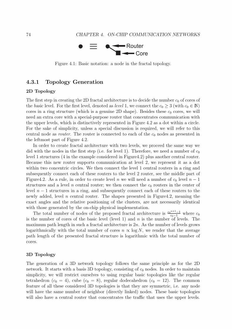
74 CHAPTER 4. ON-CHIP COMMUNICATION NETWORKS
Core
Router
Figure 4.1: Basic notation: a node in the fractal topology.
4.3.1 Topology Generation
2D Topology
The first step in creating the 2D fractal architecture is to decide the number c0 of cores ofthe basic level. For the first level, denoted as level 1, we connect the c0 ≥ 3 (with c0 ∈ N)cores in a ring structure (which is a genuine 2D shape). Besides these c0 cores, we willneed an extra core with a special-purpose router that concentrates communication withthe upper levels, which is distinctively represented in Figure 4.2 as a dot within a circle.For the sake of simplicity, unless a special discussion is required, we will refer to thiscentral node as router. The router is connected to each of the c0 nodes as presented inthe leftmost part of Figure 4.2.
In order to create fractal architecture with two levels, we proceed the same way wedid with the nodes in the first step (i.e. for level 1). Therefore, we need a number of c0level 1 structures (4 in the example considered in Figure4.2) plus another central router.Because this new router supports communication at level 2, we represent it as a dotwithin two concentric circles. We then connect the level 1 central routers in a ring andsubsequently connect each of these routers to the level 2 router, see the middle part ofFigure4.2. As a rule, in order to create level n we will need a number of c0 level n − 1structures and a level n central router; we then connect the c0 routers in the center oflevel n − 1 structures in a ring, and subsequently connect each of these routers to thenewly added, level n central router. The shapes presented in Figure4.2, meaning theexact angles and the relative positioning of the clusters, are not necessarily identicalwith those generated by the on-chip physical implementation.
The total number of nodes of the proposed fractal architecture is c0n+1−1c0−1
where c0is the number of cores of the basic level (level 1) and n is the number of levels. Themaximum path length in such a fractal architecture is 2n. As the number of levels growslogarithmically with the total number of cores n ∝ logN , we render that the averagepath length of the presented fractal structure is logarithmic with the total number ofcores.
3D Topology
The generation of a 3D network topology follows the same principle as for the 2Dnetwork. It starts with a basis 3D topology, consisting of c0 nodes. In order to maintainsimplicity, we will restrict ourselves to using regular basic topologies like the regulartetrahedron (c0 = 4), cube (c0 = 8), regular dodecahedron (c0 = 12). The commonfeature of all these considered 3D topologies is that they are symmetric, i.e. any nodewill have the same number of neighbor (directly linked) nodes. These basic topologieswill also have a central router that concentrates the traffic that uses the upper levels.

4.3. ON-CHIP FRACTAL ARCHITECTURES 75
n
c
c
= 1= 5
= 41
0
n
c
c
= 2= 21
= 42
0
n
c
c
= 3= 85
= 43
0
Figure 4.2: Fractal architecture creation procedure when c0 = 4, for n = 1, 2 and 3levels.
However, the most favorable case for the local traffic, in the sense that the shortestpaths will not go through the central routers (therefore only non-local traffic will usethe central routers), is the case of the regular tetrahedron.
The next level will be built by linking the c0 basis levels, through their central routers,by employing the same topology as for the basis, and a central upper-level router whichwill be linked to every lower central router. The next level will be generated usingthe same recursive procedure, as presented in Figure4.3 for the case of the regulartetrahedron fractal. The number of nodes in the basis level, according to the levelnumber is the same as for the 2D square-based fractal topology. The only difference isthat the local connectivity is higher, meaning a shortest path of 1 between any 2 localnodes (i.e. nodes at the same fractal level which are connected at the same centralnode). In the case of a cube, the shortest path between any 2 local nodes is 3 if weexclude the central node. If the central node is used for local traffic (a situation thatwe want to avoid), then the shortest path length becomes 2.
Static Analysis
For the fractal structures presented in Sections 4.3.1 and 4.3.1, the static characteristicsare presented under the form of average path length L, clustering coefficient C anddegree distribution P .
For the p-D fractal structures (p = 2, 3) with n levels and with c0 nodes in the basic

76 CHAPTER 4. ON-CHIP COMMUNICATION NETWORKS
n = 1
n = 3
n = 2
Figure 4.3: 3D fractal architecture creation procedure: the regular tetrahedron topologywith 1, 2, and 3 levels.

4.3. ON-CHIP FRACTAL ARCHITECTURES 77
ring, we can express the number of nodes at distance i from a given node, MpDf (i):
MpDf (i) ≃
{
pck−10 for i = 2k − 1
ck0 −∑2k−1
j=0 MpDf (j) for i = 2k
(4.1)
Having this approximation formula that excludes central nodes, we can define an upperbound for the average path length in all these fractal 2D topologies:
LpDf (n) <
1
c0n
2n∑
i=1
i ·MpDf (i) (4.2)
For the clustering coefficient it becomes more appropriate to express it for the 2D fractalstructure as in Equation 4.3.
C2Df (n) =
23cn0 (c0 − 1) + 2c0
c0+3
(
cn−10 − 1
)
+ 2
cn+10 − 1
(4.3)
At the same time, generalizing an expression for 3D clustering coefficient would beimpracticable, because performing generalization for all considered 3D shapes wouldbe too difficult. Therefore, we present the clustering coefficient for the 3D regulartetrahedron fractal structure (c0 = 4, Equation 4.4) and for the 3D cube fractal topology(c0 = 8, Equation 4.5).
C3Df−4 (n) =
(
c0n
2+ 1)
(c0 − 1) + 2c07(c0
n−1 − 1)
c0n+1 − 1(4.4)
C3Df−8 (n) =
c0n
2(c0 − 1) + 1
4(c0
n−1 − 1) + 6c0
c0n+1 − 1(4.5)
The degree distribution is given by equation 4.6:
P pDf (l) =
cn0 (c0−1)
cn+10 −1
for l = p+ 1c0−1
cn+10 −1
for l = c0c0(cn−1
0 −1)cn+10 −1
for l = c0 + p+ 1
0 for all other l
(4.6)
Equations 4.2–4.6 c0 ≥ 3 present the number of nodes in the basic-level ring, n ∈ N
is the number of levels when indexing the levels starting with 1. In equation 4.6, l ∈ N
is the degree parameter of a node.
This assessment indicates that the proposed structure is regular and clustered, whileachieving low average path length (small-world effect, SW) [143]. Also, because thistopology is self-similar it has scale-free (SF) characteristics. This aspect is furtheremphasized by the fact that if we reroute a relatively small number of long-range links,the degree distribution is brought closer to a power-law [68], as suggested in Figure4.4.
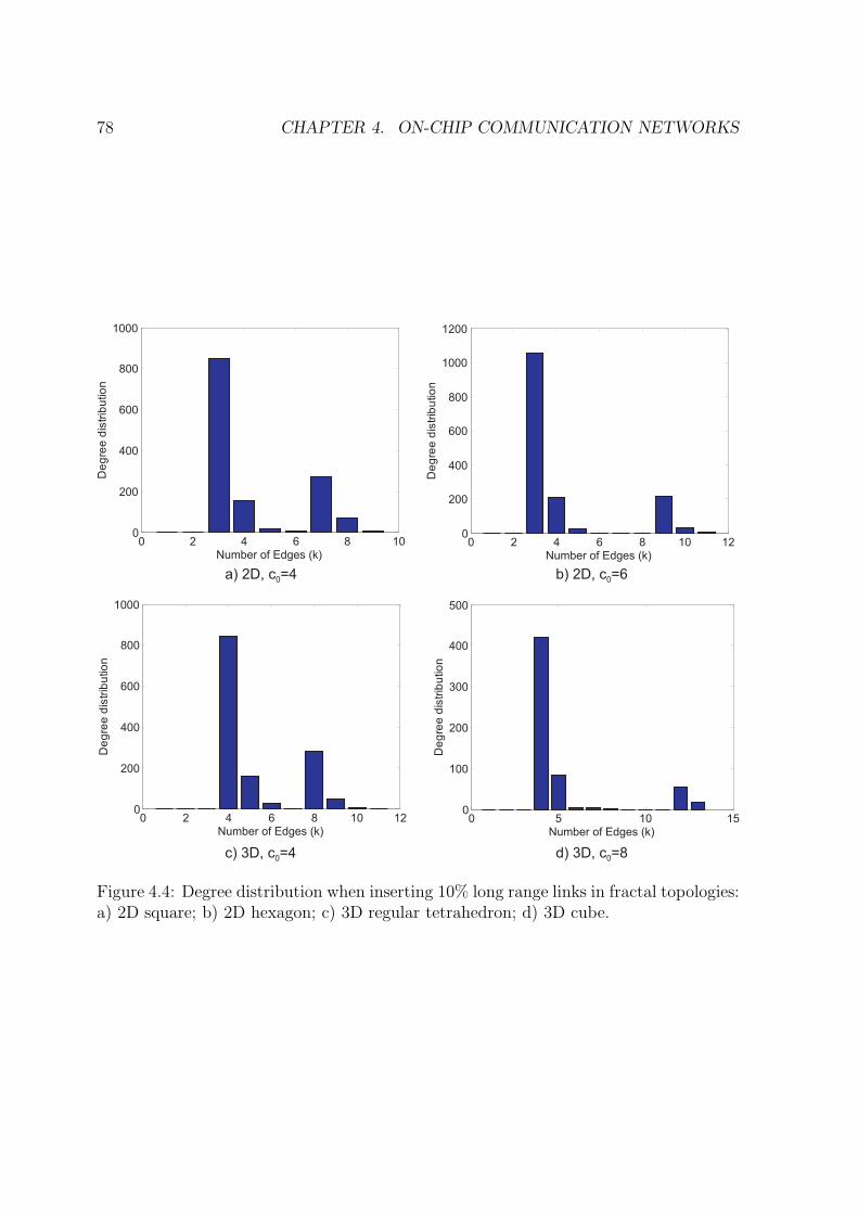
78 CHAPTER 4. ON-CHIP COMMUNICATION NETWORKS
0 2 4 6 8 10 120
200
400
600
800
1000
Number of Edges (k)
De
gre
ed
istr
ibu
tio
n
0 5 10 150
100
200
300
400
500
Number of Edges (k)
De
gre
ed
istr
ibu
tio
n
0 2 4 6 8 100
200
400
600
800
1000
Number of Edges (k)
De
gre
ed
istr
ibu
tio
n
0 2 4 6 8 10 120
200
400
600
800
1000
1200
Number of Edges (k)
De
gre
ed
istr
ibu
tio
n
a) 2D, c =40 b) 2D, c =60
c) 3D, c =40 d) 3D, c =80
Figure 4.4: Degree distribution when inserting 10% long range links in fractal topologies:a) 2D square; b) 2D hexagon; c) 3D regular tetrahedron; d) 3D cube.

4.4. RESOURCE MANAGEMENT IN FRACTAL NETWORKS 79
4.4 Resource Management in Fractal Networks
4.4.1 Routing
In a regular cartesian topology, like mesh or torus, the node indexing used for routingpurposes is performed according to cartesian node position. For our fractal topology wehave allocated indexes for each node by a simple breadth-first search in the graph, havingthe starting point at the top of the graph, and the address sequence being assigned from1 to c0
n+1−1c0−1
.Also, when dealing with the fractal network, the conventional routing mechanisms
such as the x-y routing cannot be used. Therefore, we have to look for a suitable routingmechanism, inspired by the routing strategies that were used for the somehow similarconventional structures, like quad-tree and fat-tree [187][97].
Our routing strategy first performs upward routing from the source node towardsa node that pertains to an upper cluster (i.e. c0 nodes with a router in the middle,as described in Section 4.3.1), whose central node represents a common ancestor forboth source and destination nodes. Then, when the packet arrives in this cluster, it isrouted within the cluster (local routing) towards a node that represents an ancestor forthe destination. Finally, downward routing is performed from the upper cluster nodetowards the destination node.
Local Routing
First, we have to determine the shortest path from the source to the destination. Inorder to illustrate this, we consider the general case from Figure 4.5. We first simplycheck if addressdestination = 1; if this condition is true then the destination is the centralrouter (1) which can be reached in one hop from any other cluster node. If the conditionis not true, then we compute (addresssource − addressdestination)mod c0 − c0
2which can
give one of the following outcomes:
a) 0: it means that the destination is on the opposite side, i.e. the distance from thesource to the destination is the same in both directions;
b) −x: the destination is x hops to the right, x can be any number from 1 to(
c02− 1)
;
c) +x: the destination is x hops to the left, x can be any number from 1 to(
c02− 1)
.
After determining the position of the destination relative to the source pertaining tothe same cluster (consisting of all c0 local nodes, plus their central router), we route thepacket with the following probability:
pl =
(
1− 1κ
)
·(
1− δmin
c0
)
, shortest path(
1− 1κ
)
· δmin
c0, longest path
1κ, through the router
(4.7)
Where δmin is the minimum distance from the source to the destination (δmin = c02−
| (addresssource − addressdestination)mod c0 − c02|) and κ > 1 ∈ R. The central node

80 CHAPTER 4. ON-CHIP COMMUNICATION NETWORKS
1
2
3
4
c0+1 c0
c0-1
c0-2
Source
Destination
Figure 4.5: Local routing within the basic cluster of the fractal topology. The clusterconsists of a ring of c0 nodes, linked to a central node, that allows for communicatingwith the upper levels.
is always used when communicating with the upper levels. Therefore, when dealingwith local traffic (i.e. within the cluster), it is desired not to use the central node, bymaximizing κ. Thus, we avoid congesting this central router with unnecessary localtraffic.
However, when c0 > 4, excluding the central router for local traffic leads to perfor-mance loss because the average path length within the cluster increases. This meansthat when the NoC system runs an application with highly clustered traffic, κ can besmaller because the central routers are not solicited with intense inter-level traffic.
We have 2 special cases when c0 = 3 or 4, i.e. the ring becomes a triangle and asquare respectively. For c0 = 3, the minimum distance between any two local nodes is1, without using the central node. When c0 = 4 the minimum distance between any twolocal nodes is 2, and the route can always avoid the central node. In both these cases,pl can be computed as:
p∗l =
{
1−(
1− 1κ
)
· δmin
c0, shortest path
(
1− 1κ
)
· δmin
c0, longest path
(4.8)
Upward Routing
Given a node x, its parent is given by:
parent (x) ⇐ ⌊(
x−2c0
)
+ 1⌋In order to determine a route between two nodes x and y in the network, we apply
the following deterministic algorithm:

4.4. RESOURCE MANAGEMENT IN FRACTAL NETWORKS 81
if (x+ y) 6= 2 thenwhile parent (x) 6= parent (y) doif parent (x) < parent (y) theny ⇐ parent (y)add to route y
elsex ⇐ parent (x)add to route x
end ifend while
end if
This algorithm finds a common ancestor for the source and destination, and at thesame time determines the number of levels that need to be passed from the source to thecommon ancestor; we denote this number by ls. Thus, we can describe the probabilisticrouting procedure from the source to the common ancestor, by expressing the routingprobabilities as follows in Equation 4.9:
pu =
12n·ls
same cluster (left)1
2n·lssame cluster (right)
n−1n
(
1− 1ls
)
center router (up)
(4.9)
Note that ls decreases each time we go up a level, and it will be the indicator that wehave reached the cluster of the common ancestor when ls = 1. In this situation, weperform a local routing, as described in Section 4.4.1(within the cluster that containsthe common ancestor of the source and destination).
Downward Routing
After reaching the common ancestor, we compute ld (the hop distance between thecommon ancestor and the destination node), and then start going down on the hierarchylevels, following a probabilistic route that has a similar description with the upwardrouting, as in Equation 4.10:
pd =
12n·ld
downward to the left1
2n·lddownward to the right
n−1n
(
1− 1ld
)
straight down
(4.10)
In contrast with the upward direction, here ld increases from 1 to the difference oflevels determined by the destination and the common ancestor. In the equation above,downward to the left or right means routing downward to the left or right of one of thedestination’s ancestors, whereas routing straight down means route directly to one ofthe destination’s ancestors.
Total Routing
If we want to perform total routing from anywhere in the graph, first we have to deter-mine the relative position of the destination from the source, which can be: up, down,

82 CHAPTER 4. ON-CHIP COMMUNICATION NETWORKS
or in the same cluster. If it is up, then we act as described in Section 4.4.1, if it is downthen we act as described in Section 4.4.1, i.e. the downward routing, and last, if it is inthe same cluster we follow the procedure described in Section 4.4.1.
3D Routing
In the case of the 3D structures, the basic cluster is not organized as a ring, thereforelocal routing cannot work the way it is described in Section 4.4.1. However, takinginto consideration the discussion from Section 4.3.1, the regular tetrahedron 3D fractaltopology is favorable for shortest path routing, because local traffic can always usethe shortest paths without going through the central node. In this case, given thefact that the upper levels of the structure are connected in the same way, the mostfavorable solution for regular tetrahedron fractal topology is to use deterministic routing,by determining the shortest path with Dijkstra’s algorithm [45] or some other similarefficient algorithms.
4.4.2 Dimensioning of Communication Channels
In order to preserve the spatial fractality within the overall structure, the size of thelinks between the nodes in the upper levels will have to be increased according to thenumber of that level. This observation also helps in accommodating the heavier trafficthat exists at the higher levels. The central nodes are required by the proposed fractalarchitectures, but are prone to congestion because they concentrate the traffic generatedat the lower-level nodes (and the number of lower-level nodes grows exponentially withthe number of levels).
In order to avoid these congestion situations, the natural solution is to allocate thenumber of virtual channels for links at level i according to the number of nodes atlevel i − 1. These level i − 1 nodes communicate outside their cluster through theircorresponding central nodes that pertain to level i. This number of level i− 1 nodes isequal with the number of nodes within a cluster, which is c0, while the total number oflower-level nodes communicating with upper levels through one level-i central node is
Ni =(c0)
i−1c0−1
. Therefore, if any link at level i− 1 has v virtual channels, then the size ofa link at level i will have v · s virtual channels, where s (depending on c0) is the scalingfactor which assures that the number of virtual channels grows towards the top of theproposed fractal architecture. Figure4.6 presents the scaling of the virtual channels ona 2-level fractal architecture example with clusters having c0 = 4 nodes.
The problem of selecting the scaling factor can be approached in an ad-hoc manner;if the traffic is not clustered, then the probability of packets leaving the node clustersis low, and we can avoid allocating a large number of virtual channels. However, notall applications entail clustered traffic, and so the topology has to offer support forinter-level communication, by allocating a substantial number of virtual channels at theupper levels.

4.4. RESOURCE MANAGEMENT IN FRACTAL NETWORKS 83
v =1 1
v =v s2 0
x
y
z
Figure 4.6: Allocation of channel width in terms of virtual channels, on a 2-level fractalarchitecture for c0 = 4. The number of virtual channels for the links on fractal level i isvi.
Allocating for scaling factor of c0
From a fractal geometry standpoint, this scaling factor can be related to the Hausdorff-Besicovitch (HB) fractal dimension. The HB dimension of a fractal is given by lognc
log sf,
where nc is the number of self-similar copies at each level, and sf is the scaling factorwhen generating the shapes at level i + 1, from level i. In the case of our fractaltopology, the number of self-similar copies is nc = c0. When we allocate a number ofv · c0 virtual channels for each link at level i, and each of the links at level i − 1 has vvirtual channels, the scaling factor will be s = sf = c0. Therefore, in these conditions,the Hausdorff dimension will be log c0
log c0= 1. It is a virtual channel scaling factor that
corresponds to a situation where there is a distinct set of virtual channels dedicated tocommunicating between any two nodes from the fractal topology. This case is equivalentto a totally connected network.
This virtual channel allocation – that corresponds to a fractal dimension of 1 – isideal, because it avoids packet competition for virtual channels. However it is using anexponential number of virtual channels. If the fractal topology is built on m levels andeach link at the lowest level has just 1 virtual channel, then at the highest level eachlink will have c0
m−1 virtual channels. Nonetheless, the probability of really needing thishuge communication infrastructure is small when the number of fractal levels is small.
We call local traffic communication that occurs between nodes within the same clusteron the same fractal level, as presented in the example form Figure4.6 when node xcommunicates with node y. As shown in Figure4.6, when the communication nodes donot pertain to the same cluster (e.g. node x communicates with node z), the non-localtraffic will use the upper-level links. Assuming uniform random traffic, as the probability

84 CHAPTER 4. ON-CHIP COMMUNICATION NETWORKS
of having non-local traffic (and therefore using the upper-level links) is approaching 1when the number of levels n > 3, it is expected that most of the traffic will use thevirtual channels on the upper levels. As such, in these conditions, the scaling factorwill have to correspond to a Hausdorff dimension that is closer to 1. The probability ofnon-local traffic is given in equation 4.11.
Pnl (n) =(∑n
i=1 c0i)− c0 − 1
(∑n
i=1 c0i)− 1
(4.11)
The probability of non-local traffic in fractal architectures with a basic level having3, 4, 6 and 8 nodes is presented in Figure4.7.
1 2 3 4 5 60
0.2
0.4
0.6
0.8
pnl3 n( )
pnl4 n( )
pnl6 n( )
pnl8 n( )
n
1.0
Figure 4.7: Probability of non local traffic in fractal architectures with the number oflevels n, for c0 = 3, 4, 6, and 8 nodes: pnl3(n), pnl4(n), pnl6(n), and pnl8(n) respectively.
Allocating for logarithmic scaling factor
When aiming at allocating a linear amount of virtual channels with the number of nodes,instead of looking for highly-efficient communication infrastructure, the scaling factorat level i can be set as s = ⌊ln (Ni) + 1⌋, where ⌊a⌋ denotes the largest integer thatis smaller than a. Nevertheless, this allocation procedure will use a linear number ofvirtual channels with the number of fractal levels n, as N (the total number of nodes)is exponential with n (fractal level number) and the number of virtual channels is fixedas logarithmic with N .
Equivalent mesh allocation
However, when allocating virtual channels, another valid approach consists of using ap-proximately the same number of virtual channels as the equivalent mesh architecture

4.4. RESOURCE MANAGEMENT IN FRACTAL NETWORKS 85
(i.e. the mesh that will accommodate the same number of nodes as the fractal architec-ture). This total number of virtual channels for the mesh equivalent, V Cm, is given inequation 4.12, where vm is the number of virtual channels allocated for each link in themesh.
V Cm (n) = 2 ·√
c0n+1 − 1
c0 − 1
(
√
c0n+1 − 1
c0 − 1− 1
)
· vm (4.12)
In the proposed fractal architecture, the total number of allocated virtual channels(V Cf) with the number of levels n, when the scaling factor s = c0, is given in equation4.13.
V Cf (n) = 2 · n · c0n (4.13)
When s 6= c0, the total number of virtual channels in the fractal network, V Cfs,with the number of levels n is:
V Cfs (n) = 2 · c0 · sn−1 ·(
c0s
)n − 1c0s− 1
(4.14)
At the same time, applying the virtual channel allocation according to the loga-rithmic scaling factor, entails a total number of virtual channels as given in equation4.15:
V Cah (n) = 2 · c0n++2 ·
∑n−1i=1
[
⌊ln(
c0i+1−1c0−1
− 1)
+ 1⌋c0n−i]
(4.15)
Equations 4.13 to 4.15 can be used for somputing the scaling factor so that the totalnumber of virtual channels in the fractal network is approximatively the same as for theequivalent mesh. Figure4.8 presents the case of c0 = 4, where the scaling factor s = 3will approximate the number of virtual channels from the equivalent mesh network withvm = 2.
Therefore, the virtual channel allocation for the fractal architecture (when c0 =4), so that the total number of virtual channels is approximately the same as for theequivalent mesh topology, is obtained for a scaling factor s = 3. This means that thecorresponding Hausdorff fractal dimension becomes log 4
log 3. Because the fractal dimension
> 1, it means that the network is no longer fully connected (i.e. there are no dedicatedsets of virtual channels for connecting any two nodes), and competition for virtualchannels is possible. In fact, as the fractal dimension grows, virtual channel contentionalso grows, thus affecting the communication efficiency that can be achieved when theHausdorff dimension is 1.
4.4.3 Surface Allocation
It is expected that the clustered nature of fractal topology shapes entails sparse utiliza-tion of silicon die. As such, in order to be able to assess the heat dissipation capabilitiesof such a fractal architecture, knowing how it is occupying the silicon die is of paramount

86 CHAPTER 4. ON-CHIP COMMUNICATION NETWORKS
1 2 3 4 50
2000
4000
6000
VCm4 n( )
VCf44 n( )
VCfs43 n( )
VCah4 n( )
n
Figure 4.8: Network comparison in terms of total virtual channel number: V Cf44 virtualchannels for the fractal architecture where c0 = s = 4, V Cf43 for c0 = 4 and s = 3,V Cah4 for the logarithmic scaling factor allocation procedure when c0 = 4, and V Cm4
for the mesh equivalent of a fractal network where c0 = 4 and vm = 2.
importance. To this end, we will use four parameters for the n-level fractal architecture:one that indicates the area required by the nodes or vertices (router+core) (Vn), anotherthat indicates the area of the links (Kn), one that indicates the area used for both nodelogic and links (An), and the last one expressing the total silicon area (Sn). An obviousobservation is that An < Vn+Kn, as some of the node and link surfaces are overlappingfrom a geometric point of view.
This analysis starts from the base level 1 of a 2D fractal topology with c0 = 4 fromFigure4.2, as presented in Figure4.9, where the square allocated for the node has a λ
3
edge, the thickness of the link is γ and the entire block is included within a λ×λ square.The values for the 4 parameters in our analysis are given, for the first level, in Equation
l
g
gl
Level 1
l/3
l/3
l/3
l/3 l/3 l/3
Figure 4.9: Level 1 fractal square architecture: the black squares represent the surfaceallocated to the nodes, whereas the colored lines represent the links.

4.4. RESOURCE MANAGEMENT IN FRACTAL NETWORKS 87
4.16.V1 = 5
(
λ3
)2
K1 =43
(
2 +√2)
γλ
A1 = 5(
λ3
)2+ 4
3γλ
S1 = λ2
(4.16)
For the second level, see Figure4.10, we considered that the thickness of links con-necting the nodes from the upper level will grow with a factor α. Also, the center nodespertaining to the upper levels will occupy half of the center square surface (the blackλ2× λ
2in the middle of Figure4.10. The values of the 4 parameters, in a 2-level fractal
l
3ll
l
g
g g
ag
l l l
3l
Level 2
l/4
l/4
l/4
l/4
l/3
l/3
l/3
Figure 4.10: Surface allocation for level 2 fractal square architecture.
structure corresponding to Figure4.10 are given in Equation 4.17.
V2 = 4V1 +(
λ2
)2
K2 = 4K1 + 8γλ+ 4√2αγλ
A2 = 4A1 + 453γλ+
√2αγλ+
(
λ2
)2
S2 = (3λ)2
(4.17)
It can be proven that for any i > 1 we have:
Vi+1 = 4Vi +(
3i λ2
)2
Ki+1 = 4Ki + 4 · 3i√2αi+1γλ+ 8 · 3iαiγλ
Ai = 4Ai +√23iαi+1γλ+ 4 · 3iαiγλ+
+8 · 3i−1αi−1γλ+(
3i λ2
)2
Si+1 = (3i+1λ)2
(4.18)

88 CHAPTER 4. ON-CHIP COMMUNICATION NETWORKS
Having first level parameters V1, K1, A1 and S1 from Equation 4.16, and the recursiverelations from Equation 4.18, we obtain that at level n we have:
Vn = 4n{
V1 +λ2
20
[(
94
)n − 1]
}
Kn = 4n[
K1 +(
2 +√2α) ( 3
4α)
n−1
34α−1
γλ
]
An = 4nA1 + 4n−1(
4 + α√2) ( 3
4α)
n−1
34α−1
γλ+
+2 · 4n−1 (34α)
n−1−1
34α−1
γλ+
+83· 4n−1γλ+
( 94)
n−1
5· 4n−1λ2
Sn = (3nλ)2
(4.19)
The parameters from equations 4.19 can be used to compute the ratios given bythe surface required by the nodes (core+router), the links and nodes+links, versus thetotal surface: Vn/Sn, Kn/Sn, and An/Sn respectively. These ratios are represented inFigure4.11, for the example case of λ = 3, γ = λ
20, and α = 2.
1 2 3 4 5 6 70
0.05
0.1
0.15
0.2
0.25
0.3
0.35
0.4
n (number of levels)
ratio
V/S (cores)K/S (links)A/S (total area)
Figure 4.11: Ratio of surface occupancy for nodes V/S, links K/S, and nodes+linksA/S versus the number of levels n.
The plot in Figure4.11 shows that the area utilization decreases exponentially withthe number of fractal levels, as the fractal structure becomes more sparse, thus facili-tating heat dissipation.
4.5 Conclusion
Using complex network science in order to optimize on-chip multiprocessor communica-tion networks is indeed a very promising research topic. As NoC communication entails

4.5. CONCLUSION 89
dealing with complex emerging phenomena, the solutions for optimizing NoC architec-tures will have to find inspiration in the new science of complexity, including statisticalphysics and complex networks.
We note that there are still many difficulties ahead, as current fabrication technol-ogy is fundamentally limiting what can actually be implemented in Silicon (includingfractal or complex network topologies). Indeed, from a technological standpoint, onlyregular structures are supported, while long-range interconnections are hard to build.However, new on-chip communication technologies such as optical [201][202] or wirelesscommunication [89][115] offer new hope for overcoming the above-mentioned difficulties.As such, we intend to further pursue research on this topic, by adapting the complexnetwork tools to the new NoC communication technologies.

90 CHAPTER 4. ON-CHIP COMMUNICATION NETWORKS

Chapter 5
Conclusions
The present thesis argues that there is fertile ground for research at the frontiers betweencomputer engineering, information technology, physics, medical and social sciences. In-deed, the advent of big data techniques such as machine and deep learning or complexnetworks have spurred significant advances in scientific fields like physics, biology, preci-sion medicine, genomics, social networks and social physics, emergent human behaviormodeling, etc. Moreover, there are strong reasons which indicate the new network sci-ence as a reliable source of solutions for engineering problems, ranging from managingcomplexity in NoC communication to designing power grids or controlling road traffic.Our thesis shows how the new science of complex networks can be used for optimiz-ing NoC communication, modeling opinion dynamics in social networks, and precisionmedicine (drug repositioning and uncovering disease phenotypes).
However, in order to perform big data approaches, we need lots of relevant dataon physical processes, human activity, or human physiological signals. To this end,computer engineering can provide solutions and tools such as Internet of Things (IoT)or Cyber Physical Systems (CPS): a lot of sensors gather big amounts of data to beanalyzed and then used for computation, communication and control. Following thistrend, it can be said that we entered the new era of inexact computation [128], whichis characterized by integrating the computer in complex physical, biological, social andprocesses.
To this end, within UEFISCDI’s PN-III-CERC-CO-PED-2016 framework, we pro-posed as coordinator the research project entitled ”Internet of Things Meets ComplexNetworks for Early Prediction and Management of Chronic Obstructive PulmonaryDisease”, or Internet of thiNgs Complex nEtworks PredicTION (INCEPTION). Themotivation for our proposal is that recent research indicates Chronic Obstructive Pul-monary Disease (COPD) as the third cause of death and one of the main impedimentsfor the quality of living in todays society. COPD is defined as the clinical conditionwhich reduces pulmonary capacity; it is not reversible, however if diagnosed at an earlyphase, its evolution can be controlled. Unfortunately, early detection of COPD is a dif-ficult task, and often time people are diagnosed when they are already in an advancedstage. Capitalizing on recent research results which indicate sensor systems, mobile,and Internet of Things solutions as very useful for monitoring and managing COPD,we propose a personal, integrated prototype system for early detection and evolution
91

92 CHAPTER 5. CONCLUSIONS
prediction of COPD. As such, we intend to build a sensor network that gathers multiplephysiological signals, and a mobile application that extracts the multi-fractal spectraas mere signatures of these signals. Then, the mobile system will integrate the physio-logic signatures with anthropometric and other individual clinical data. The overviewof INCEPTION at individual level is presented in Figure 5.1.
Pulse oximeter sensors:
pulse rate and
oxygen saturation
Heart sensors:
electrocardiogram,
phonocardiogram,
electromyogram
Humidity and
pressure
sensors:
breathing
rate
Air pressure
sensor:
spirometry
Electrical sensors:
encephalogramSmartphone: physiological
signals gathering (via
bluetooth) and processing
Anthropometric
and clinical parameters:
• age, gender, BMI
• comorbidities, medication
• smoking status, smoking score
• number of exacerbations
• COPD onset
• questionnaire results (CAT, MRC)
COPD
stage prediction
Figure 5.1: Overview of INCEPTION at individual-level. Physiological signals are gath-ered with a sensor network and transmitted via Bluetooth. Anthropometric and clinicalparameters are recorded and integrated at smartphone-level and then sent over the cloudin a centralized database.
On the server side, we will collect the integrated data from a population of individ-uals, to build a complex network model of patients. Indeed, recent papers indicate thecomplex network model as very useful for generating COPD predictions. To this end, wewill employ modularity clustering and network layout tools to build prediction modelsfor both early detection and evolution prediction of COPD. he overview of INCEPTIONat individual level is presented in Figure 5.2.
The prediction model will be instantiated as a smartphone application and testedin order to assess its predictive capacity. In order to undertake the objectives of ourproposal, we assemble a multidisciplinary team, consisting of computer engineers (hard-ware and software) and specialized medical doctors from University of Medicine andPharmacy ”Victor Babes” Timisoara. Our computer engineering teams will build thehardware and software parts of our demonstration model, whereas the medical teamwill provide the necessary medical expertise, in order to test and validate the modelproposed by the computer engineers.

93
Figure 5.2: Overview of INCEPTION at server-level. Integrated individual data arecollected from many individuals and stored in a centralized database. The gathereddataset is then processed according to the complex network paradigm, in order to findnew pathophysiological correlations.

94 CHAPTER 5. CONCLUSIONS

Part III
Relevant Bibliography
95


Bibliography
[1] D. Acemoglu, and A. Ozdaglar, Opinion dynamics and learning in social networks,Dynamic Games and Applications 1, 1, 3-49, 2011
[2] D. Acemoglu, A. Ozdaglar, and E. Yildiz, Diffusion of innovations in social net-works, 50th IEEE Conference on Decision and Control and European Control Con-ference (CDC-ECC), pp. 2329-2334, 2011
[3] D. Acemoglu, G. Como, F. Fagnani, and A. Ozdaglar, Opinion fluctuations anddisagreement in social networks, Mathematics of Operations Research 38, 1, 1–27,2013
[4] R. Albert, and A-L. Barabasi, Statistical mechanics of complex networks, Reviewsof modern physics, 74, 1, 47, 2002
[5] F. Alkemade, and C. Castaldi, Strategies for the diffusion of innovations on socialnetworks, Computational Economics, 25, 1-2, 3-23, 2005
[6] C. Alt, O. Astrachan, J. Forbes, R. Lucic, and S. Rodger, Social networks generateinterest in computer science, ACM SIGCSE Bulletin, 38, 1, 438-442, 2006
[7] L. Amaral, A. Scala, M. Barthelemy, and H.E. Stanley, Classes of small-worldnetworks, Proceedings of the National Academy of Sciences, 97, 21, 11149-11152,2000
[8] R.M. Anderson, R.M. May, and B. Anderson, Infectious diseases of humans: dy-namics and control, Wiley Online Library 28, 1992
[9] T. Arentze, and H. Timmermans, Social networks, social interactions, and activity-travel behavior: A framework for microsimulation, Environment and planning. B,Planning & design, 35, 6, 1012, 2008
[10] T. Arentze, P. van den Berg, and H. Timmermans, Modeling social networks ingeographic space: approach and empirical application, Environment and Planning-Part A, 44, 5, 1101, 2012
[11] D. Auber, Tulip: A huge graph visualization framework, Graph Drawing Software,Springer, 105-126, 2004
[12] R. Axelrod, The dissemination of culture a model with local convergence and globalpolarization, Journal of conflict resolution 41, 2, 203-226, 1997
97

98 BIBLIOGRAPHY
[13] F. Bagnoli, F. Franci, and R. Rechtman, Opinion formation and phase transitionsin a probabilistic cellular automaton with two absorbing states, Cellular Automata,Springer, pp. 249-258, 2002
[14] N.T.J. Bailey et al., The mathematical theory of infectious diseases and its applica-tions, Charles Griffin & Company Ltd, 5a Crendon Street, High Wycombe, BucksHP13 6LE., 1975
[15] S. Bandyopadhyay, A.R. Rao, B. Sinha, and B.K. Sinha, Models for Social Networkswith Statistical Applications, Sage, Vol.13, 2011
[16] A.L. Barabasi, Network science, Cambridge University Press, 2016
[17] A.L. Barabasi, The network takeover, Nature Physics, 8, 1, 14, 2011
[18] A.L. Barabasi, and R. Albert, Emergence of scaling in random networks, Science286, 5439, 509-512, 1999
[19] M. Bastian, S. Heymann, and M. Jacomy, Gephi: an open source software forexploring and manipulating networks. ICWSM, 2009
[20] V. Batagelj, and A. Mrvar, Pajek-program for large network analysis, Connections21, 2, 47-57, 1998
[21] M. A. Bender, D. P. Bunde, E. D. Demaine, S. P. Fekete, V. J. Leung, H. Meijer,C. A. Phillips, Communication-Aware Processor Allocation for Supercomputers:Finding Point Sets of Small Average Distance, C Algorithmica 50, 2, 279-298, 2008
[22] G. B. P. Bezerra, S. Forrest, M. Forrest, A. Davis, P. Zarkesh-Ha, Modeling NoCtraffic locality and energy consumption with rent’s communication probability dis-tribution, In Proc. 12th ACM/IEEE Intl. Workshop on System Level InterconnectPrediction, New York, NY, USA, pp. 3-8, 2010
[23] A. Bigdeli, A. Tizghadam, and A. Leon-Garcia, Comparison of network criticality,algebraic connectivity, and other graph metrics, Proceedings of the 1st Annual ACMWorkshop on Simplifying Complex Network for Practitioners, 4, 2009
[24] K.R. Bisset, J. Chen, X. Feng, V.S. Kumar, and M.V. Marathe, EpiFast: a fastalgorithm for large scale realistic epidemic simulations on distributed memory sys-tems, Proceedings of the 23rd ACM International Conference on Supercomputing,pp. 430-439, 2009
[25] S. Biswas, A.K. Chandra, A. Chatterjee, and B.K. Chakrabarti, Phase transitionsand non-equilibrium relaxation in kinetic models of opinion formation, Journal ofPhysics: Conference Series 297, 1, 012004, 2011
[26] P. Bogdan, R. Marculescu, Statistical physics approaches for network-on-chip trafficcharacterization, In Proc. 7th IEEE/ACM Intl. Conference on Hardware/SoftwareCodesign and System Synthesis (CODES+ISSS ’09), New York, NY, USA, pp.461-470, 2009

BIBLIOGRAPHY 99
[27] P. Bogdan, M. Kas, R. Marculescu, O. Mutlu, QuaLe: a quantum-leap inspiredmodel for non-stationary analysis of NoC traffic in chip multi-processors, In Proc.ACM/IEEE Intl. Symp. on Networks-on-Chip (NOCS), pp. 241-248, 2010
[28] B. Bolgar et al., Drug repositioning for treatment of movement disorders: fromserendipity to rational discovery strategies, Current topics in medicinal chemistry13, 2337–2363, 2013
[29] E. Bolotin, I. Cidon, R. Ginosar, A. Kolodny, Routing table minimization for ir-regular mesh NoCs, In Proc. Design Automation and Test in Europe (DATE), pp.942-947, 2007
[30] J. Borondo, F. Borondo, C. Rodriguez-Sickert, C.A. Hidalgo, To each according toits degree: The meritocracy and topocracy of embedded markets, Scientific Reports,4, 3784, 2014
[31] C.T. Butts, Social network analysis with SNA, Journal of Statistical Software 24,6, 1-51, 2008
[32] A. Cairns, G. Poulos, and R. Bogan, Sex differences in sleep apnea predictors andoutcomes from home sleep apnea testing, Nature and Science of Sleep, 8, 197, 2016
[33] N. Caseiro, and P. Trigo, Comparing complex networks: An application to emer-gency managers mental models, Third Brazilian Workshop on Social Simulation(BWSS), pp. 128-131, 2012
[34] D. Centola, The spread of behavior in an online social network experiment, Science329, 5996, 1194–1197, 2010
[35] D. Centola, and M. Macy, Complex contagions and the weakness of long ties1,American Journal of Sociology 113, 3, 702-734, 2007
[36] K. Channakeshava, K. Bisset, V.S.A. Kumar, M. Marathe, and S. Yardi, Highperformance scalable and expressive modeling environment to study mobile malwarein large dynamic networks, IEEE International Parallel & Distributed ProcessingSymposium (IPDPS), pp. 770–781, 2011
[37] H.F. Chau, C.Y. Wong, F.K. Chow, and C-H.F. Fung, Social judgment theorybased model on opinion formation, polarization and evolution, Physica A: StatisticalMechanics and its Applications 415, 770-781, 2014
[38] X.-Q. Chen, M.D. Antman, C. Gesenberg, O.S. Gudmundsson, Discovery pharma-ceuticschallenges and opportunities, The AAPS journal 8, E402–E408, 2006
[39] G. Chen, X. Wang, and X. Li, Fundamentals of Complex Networks: Models, Struc-tures and Dynamics, John Wiley & Sons, 2014
[40] N.R. Clark, K. Hu, E.Y. Chen, Q. Duan, and A. Maayan, CharacteristicDirection Approach to Identify Differentially Expressed Genes, arXiv preprintarXiv:1307.8366, 2013

100 BIBLIOGRAPHY
[41] J.J. Clarkson, Z.L. Tormala, D.D. Rucker, and R.G. Dugan, The malleable influenceof social consensus on attitude certainty, Journal of Experimental Social Psychology49, 6, 1019–1022, 2013
[42] H. Claussen, W. Lichtner, L. Heres, P. Lahaije, and J. Siebold, GDF, a proposedstandard for digital road maps to be used in car navigation systems, IEEE VehicleNavigation and Information Systems Conference, pp. 324-330, 1989
[43] P. R. Cohen, Darpa’s big mechanism program, Physical biology 12, 045008, 2015
[44] F. S. Collins, and H. Varmus, A new initiative on precision medicine, New EnglandJournal of Medicine, 372, 9, 793–795, 2015
[45] T. H. Cormen, C. E. Leiserson, R. L. Rivest, C. Stein, Introduction to Algorithms(Second ed.)Section 24.3: Dijkstra’s algorithm, MIT Press and McGraw-Hill, pp.595-601, 2001
[46] J. Chang, E. Blazek, M. Skowronek, L. Marinari, and R. P. Carlson, The antiinflam-matory action of guanabenz is mediated through 5-lipoxygenase and cyclooxygenaseinhibition, European journal of pharmacology 142, 197–205, 1987
[47] E. Chautard, N. Thierry-Mieg, and S. Ricard-Blum, Interaction networks: fromprotein functions to drug discovery. A review, Pathologie Biologie 57, 324–333,2009
[48] Y.W. Chen, L.F. Zhang, J.P Huang, The Watts–Strogatz network model developedby including degree distribution: theory and computer simulation, Journal of PhysicsA: Mathematical and Theoretical 40, 29, 8237, 2007
[49] C.-Y. Cheng, Y.-C. Lin, J.-S. Chen, C.-H. Chen, and S. Deng, Cisplatin-inducedacute hyponatremia leading to a seizure and coma: a case report, Chang Gung MedJ 34, 48–51, 2011
[50] F. Chung, B. Yegneswaran, P. Liao, S.A. Chung, S. Vairavanathan, S. Islam,A. Khajehdehi, and C.M. Shapiro, STOP Questionnaire. A Tool to Screen Patientsfor Obstructive Sleep Apnea, The Journal of the American Society of Anesthesiol-ogists, 108, 5, 812–821, 2008
[51] F. Chung, B. Yegneswaran, P. Liao, S.A. Chung, S. Vairavanathan, S. Islam,A. Khajehdehi, and C.M. Shapiro, Validation of the Berlin questionnaire and Amer-ican Society of Anesthesiologists checklist as screening tools for obstructive sleep ap-nea in surgical patients, The Journal of the American Society of Anesthesiologists,108, 5, 822–830, 2008
[52] F. Chung, Y. Yang, R. Brown, and P. Liao, Alternative scoring models of STOP-Bang questionnaire improve specificity to detect undiagnosed obstructive sleep ap-nea, Journal of Clinical Sleep Medicine, 10, 9, 951–958, 2014

BIBLIOGRAPHY 101
[53] B. M. Conti-Fine, M. Milani, and H. J. Kaminski, Myasthenia gravis: past, present,and future, The Journal of clinical investigation 116, 2843–2854, 2006
[54] L. Costa, F.A. Rodrigues, G. Travieso, and P.R. Villas Boas, Characterization ofcomplex networks: A survey of measurements, Advances in Physics 56, 1, 167-242,2007
[55] G. Csanyi, and B. Szendroi, Structure of a large social network, Physical Review E69, 3, 036131, 2004
[56] G. Csardi, and T. Nepusz, The igraph software package for complex network re-search, InterJournal, Complex Systems 5, 1695, 2006
[57] P. Csermely, T. Korcsmaros, H. J. Kiss, G. London, and R. Nussinov, Structureand dynamics of molecular networks: a novel paradigm of drug discovery: a com-prehensive review, Pharmacology & therapeutics 138, 333–408, 2013
[58] A. D’Andrea, F. Ferri, and P. Grifoni, An overview of methods for virtual socialnetworks analysis, Computational Social Network Analysis, Springer, 3-25, 2010
[59] L. Daqing, K. Kosmidis, A. Bunde, S. Havlin, Dimension of spatially embeddednetworks, Nature Physics 7, 481484, 2011
[60] A. Das, S. Gollapudi, and K. Munagala, Modeling opinion dynamics in social net-works, Proceedings of the 7th ACM international conference on Web search anddata mining, pp. 403-412, 2014
[61] G. Deffuant, D. Neau, F. Amblard, and G. Weisbuch, Mixing beliefs among inter-acting agents, Advances in Complex Systems 3, 01n04, 87-98, 2000
[62] D. De Martino, L. Dall’Asta, G. Bianconi, M. Marsili, Congestion phenomena oncomplex networks, Phys. Rev. E 79, 1, 015101, 2009
[63] L. Deng, Y. Liu, and F. Xiong, An opinion diffusion model with clustered earlyadopters, Physica A: Statistical Mechanics and its Applications 392, 17, 3546-3554,2013
[64] A. Dharmarajan, and T. Velmurugan, Lung cancer data analysis by k-means andfarthest first clustering algorithms, Indian Journal of Science and Technology, 8, 15,2015
[65] M. Dickson, and J. P. Gagnon, The cost of new drug discovery and development,Discovery Medicine 4, 172–179, 2009
[66] D. Diez, A. Augusti, C.E. Wheelock, Network analysis in the investigation ofchronic respiratory diseases. From basics to application, American Journal on Res-piratory and Critical Care Medicine 190, 981988, 2014

102 BIBLIOGRAPHY
[67] M.J. Divo, C. Casanova, J.M. Marin, V.M. Pinto-Plata, J.P. de-Torres, J.J. Zulueta,C. Cabrera, J. Zagaceta, P. Sanchez-Salcedo, J. Berto, R. Baz Davila, A.B. Alcaide,C. Cote, B.R. Celli, Chronic obstructive pulmonary disease comorbidities network,European Respiratory Journal, 46, 3, 640-650, 2015
[68] S. N. Dorogovtsev, J. F. F. Mendes, A. N. Samukhin, A. T. Zyuzin,Organizationof modular networks, In Phys. Rev. E, 78, 5, 056106, 2008
[69] S. N. Dorogovtsev, A. V. Goltsev, J. F. F. Mendes, Critical phenomena in complexnetworks, Reviews of Modern Physics Vol. 80, pp.1275-1335, 2008
[70] A. Duma, and A. Topirceanu, A network motif based approach for classifying onlinesocial networks, 9th IEEE International Symposium on Applied ComputationalIntelligence and Informatics (SACI), pp. 311-315, 2014
[71] W. J. Egan, G. Zlokarnik, and P. D. Grootenhuis, In silico prediction of drug safety:despite progress there is abundant room for improvement, Drug Discovery Today:Technologies 1, 381–387, 2004
[72] D. Elkind, Egocentrism in adolescence, Child development, pp. 1025-1034, 1967
[73] J. Ellson, E. Gansner, L. Koutsofios, S.C. North, and G. Woodhull, Graphviz: opensource graph drawing tools, Graph Drawing, Springer, pp. 483-484, 2002
[74] P. Erdos, and A. Renyi, On the evolution of random graphs, Publications del’Institut des Mathematiques Appliquees de l’Academie des Sciences de Hongrie5, 17-61, 1960
[75] E. Estrada, The structure of complex networks, Oxford University Press, 2011
[76] K. Falconer, Fractal geometry: mathematical foundations and applications Wiley,2007
[77] W. Fan, and K.H. Yeung, Online social networks: Paradise of computer viruses,Physica A: Statistical Mechanics and its Applications 390, 2, 189-197, 2011
[78] R. Faner, T. Cruz, A. Lopez-Giraldo, A. Agust, Network medicine, multimorbidityand the lung in the elderly, European Respiratory Journal 44, 3, 775788, 2014
[79] R. Faner, A. Agust, Multilevel, Dynamic Chronic Obstructive Pulmonary DiseaseHeterogeneity. A Challenge for Personalized Medicine, Annals of the AmericanThoracic Society 13, 5, 2016
[80] H. Fang, J. Zhang, and N.M. Thalmann, A trust model stemmed from the diffusiontheory for opinion evaluation, Proceedings of the 2013 international conference onautonomous agents and multi-agent systems, pp. 805-812, 2013
[81] R.J. Farney, B.S. Walker, R.M. Farney, G.L. Snow, and J.M. Walker, The STOP-Bang equivalent model and prediction of severity of obstructive sleep apnea: relationto polysomnographic measurements of the apnea/hypopnea index, Journal of ClinicalSleep Medicine, 7, 5, 459–465, 2011

BIBLIOGRAPHY 103
[82] B. S. Feero and P. P. Pande, Networks-on-Chip in a Three-Dimensional Environ-ment: A Performance Evaluation, IEEE Trans. Comput. 58, 1, pp.32-45, 2009
[83] L. Feng, Y. Hu, B. Li, H.E. Stanley, S. Havlin, and L.A. Braunstein, Competing forAttention in Social Media under Information Overload Conditions, arXiv preprintarXiv:1410.1668, 2014
[84] J. Fischer, Z. Dogas, C. Bassetti, S. Berg, L. Grote, P. Jennum, P. Levy, S. Mihai-cuta, L. Nobili, D. Riemann, F.J. Puertas-Cuesta, F. Raschke, D.J. Skene, N. Stan-ley, D. Pevernagie, and Executive Committee (EC) of the Assembly of the NationalSleep Societies (ANSS); Board of the European Sleep Research Society (ESRS),Regensburg, Germany, Standard procedures for adults in accredited sleep medicinecentres in Europe, Journal of Sleep Research, 21(4), 357–368, 2012
[85] G. Fowler, Facebook: One billion and counting, The Wall Street Journal, B1, 2012
[86] A. Fronczak, P. Fronczak, J. A. Holyst, Average path length in random networks,Physical Review E - Statistical, Nonlinear and Soft Matter Physics, 70(5 Pt 2),056110, 2004
[87] T.M.J. Fruchterman, and E.M. Reingold, Graph drawing by force-directed place-ment, Software: Practice and experience 21, 11, 1129–1164, 1991
[88] M. Gaertler, Clustering. Network Analysis, Lecture Notes in Computer ScienceLNCS 3418, pp. 178215, 2005
[89] A. Ganguly, K. Chang, S. Deb, P.P. Pande, B. Belzer, and C. Teuscher, Scal-able Hybrid Wireless Network-on-Chip Architectures for Multicore Systems, IEEETransactions on Computers, 60(10), 1485-1502, 2011
[90] I.E. Gabbay, and P. Lavie, Age-and gender-related characteristics of obstructivesleep apnea, Sleep and Breathing, 16, 2, 453–460, 2012
[91] S. Geven, J. Weesie, and F. van Tubergen, The influence of friends on adolescentsbehavior problems at school: The role of ego, alter and dyadic characteristics, SocialNetworks 35, 4, 583-592, 2013
[92] S. D. Ghiassian, et al., Endophenotype network models: Common core of complexdiseases, Scientific reports 6, 27414, 2016
[93] M. Girvan, M.E.J. Newman, Community structure in social and biological networks,Proceedings of the National Academy of Sciences, 99, 12, 7821-7826, 2002
[94] J. Golbeck, Analyzing the Social Web, Elsevier, 2013
[95] A. Graul, E. Cruces, and M. Stringer, The year’s new drugs & biologics, 2013: PartI, Drugs Today (Barc) 50, 51–100, 2014

104 BIBLIOGRAPHY
[96] D. Greenfield, S. W. Moore, Brief announcement: fractal communication in soft-ware data dependency graphs, Proc. Ann. Symp. on Parallelism in algorithms andarchitectures (SPAA), pp.116-118, 2008
[97] P. Guerrier, A. Greiner, A generic architecture for on-chip packet-switched inter-connections, In Proc. Design Automation and Test in Europe (DATE), pp. 250-256,2000
[98] A. Guille, H. Hacid, C. Favre, and D.A. Zighed, Information diffusion in onlinesocial networks: a survey, ACM SIGMOD Record 42, 2, 17-28, 2013
[99] R. Guimera, A. Diaz-Guilera, F. Vega-Redondo, A. Cabrales, A. Arenas, OptimalNetwork Topologies for Local Search with Congestion, In Phys. Rev. Lett., 89, 24,248701, 2002
[100] M. Hall, E. Frank, G. Holmes, B. Pfahringer, P. Reutemann, and I.H. Witten, TheWEKA data mining software: an update, ACM SIGKDD explorations newsletter,11, 1, 10–18, 2009
[101] J. Hedner, L. Grote, M. Bonsignore, W. McNicholas, P. Lavie, G. Parati, P. Sliwin-ski, F. Barbe, W. De Backer, P. Escourrou, I. Fietze, J.A. Kvamme, C. Lombardi,O. Marrone, J.F. Masa, J.M. Montserrat, T. Penzel, M. Pretl, R. Riha, D. Roden-stein, T. Saaresranta, R. Schulz, R. Tkacova, G. Varoneckas, A. Vitols, H. Vrints,and J. Zielinski, The European sleep apnoea database (ESADA): report from 22European sleep laboratories, European Respiratory Journal, 38, 3, 635–642, 2011
[102] R. Hegselmann, and U. Krause, Opinion dynamics and bounded confidence models,analysis, and simulation, Journal of Artificial Societies and Social Simulation 5, 3,2002
[103] C. Hernandez, F. Silla, J. Duato, A methodology for the characterization of processvariation in NoC links, In Proc. Design Automation and Test in Europe (DATE),Leuven, Belgium, pp.685-690, 2010
[104] M. Hirohashi, K. Takasuna, Y. Kasai, C. Usui, and H. Kojima, Pharmacologicalstudies with the alpha 2-adrenoceptor antagonist midaglizole. Part II: Central andperipheral nervous systems, Arzneimittel-Forschung 41, 19–24, 1991
[105] J. Huang et al., Systematic prediction of pharmacodynamic drug-drug interactionsthrough protein-protein-interaction network, PLoS Comput Biol 9, e1002998, 2013
[106] O. Hussain, Z. Anwar, S. Saleem, F. Zaidi, et al., Empirical Analysis of Seed Se-lection Criterion in Influence Mining for Different Classes of Networks, ASONAM,pp. 1-8, 2013
[107] M. A. Javarone, and T. Squartini, Conformism-driven phases of opinion formationon heterogeneous networks: the q-voter model case, ArXiv 2014arXiv1410.7300J,2014

BIBLIOGRAPHY 105
[108] M. Jacomy, T. Venturini, S. Heymann, and M. Bastian, ForceAtlas2, a continu-ous graph layout algorithm for handy network visualization designed for the Gephisoftware, PloS one, 9, 6, e98679, 2014
[109] L. Jian-Guo, D. Yan-Zhong, W. Zhong-Tuo, Multistage random growing small-world networks with power-law degree distribution, Chinese Physics Letters, 23, 3,746, 2006
[110] S.A. Joosten, K. Hamza, S. Sands, A. Turton, P. Berger, and G. Hamilton, Phe-notypes of patients with mild to moderate obstructive sleep apnoea as confirmed bycluster analysis, Respirology, 17, 1, 99–107, 2012
[111] M. Karlgren, et al., In vitro and in silico strategies to identify OATP1B1 inhibitorsand predict clinical drug–drug interactions, Pharmaceutical research 29, 411–426,2012
[112] K. Kawaguchi, Y. Oribe, and H. Uzawa, Tolbutamide effect on cultured humanendothelial cells with special reference to platelet aggregation, The Tohoku journalof experimental medicine 141, 563–568, 1983
[113] D. Kempe, J. Kleinberg, and E. Tardos, Maximizing the spread of influence througha social network, Proceedings of the ninth ACM SIGKDD international conferenceon Knowledge discovery and data mining, pp. 137-146, 2003
[114] K.-T. Khaw, and E. Barrett-Connor, Dietary potassium and stroke-associated mor-tality, New England Journal of Medicine 316, 235–240, 1987
[115] R.G. Kim, W. Choi, G. Liu, E. Mohandesi, P.P. Pande, D. Marculescu, andR. Marculescu, Wireless NoC for VFI-Enabled Multicore Chip Design: Perfor-mance Evaluation and Design Trade-Offs, IEEE Transactions on Computers, 65(4),1323-1336, 2016
[116] T. M. Laidlaw, et al., Cysteinyl leukotriene overproduction in aspirin-exacerbatedrespiratory disease is driven by platelet-adherent leukocytes, Blood 119, 3790–3798,2012
[117] K. C. Lee, and D. C. Randall, Potentiation of the pressor response to stress bytolbutamide in dogs, Integrative physiological and behavioral science, 28, 22–28,1993
[118] S. -J. Lee, K. Lee, H. -J. Yoo,Analysis and Implementation of Practical, Cost-Effective Networks on Chips, IEEE Des.Test 22, 5, 422-433, 2005
[119] C. E. Leiserson, Fat-trees: universal networks for hardware-efficient supercomput-ing, In Interconnection Networks for High-Performance Parallel Computers, IEEEComputer Society Press, pp. 170-179, 1994
[120] P. Levy, M. Kohler, W.T. McNicholas, F. Barbe, R.D. McEvoy, V.K. Somers,L. Lavie, J.-L. Pepin, Obstructive sleep apnoea syndrome, Nature Reviews. DiseasePrimers 1, 15015–15015, 2014

106 BIBLIOGRAPHY
[121] L. Lewis, Drug–drug interactions: is there an optimal way to study them?, Britishjournal of clinical pharmacology 70, 781–783, 2010
[122] L. Li, A. Scaglione, A. Swami, and Q. Zhao, Trust, opinion diffusion and radical-ization in social networks, Conference Record of the Forty Fifth IEEE Conferenceon Signals, Systems and Computers (ASILOMAR), pp. 691-695, 2011
[123] J. Li, S. Zheng, B. Chen, A.J. Butte, S.J. Swamidass, and Z. Lu, A survey of cur-rent trends in computational drug repositioning, Briefings in Bioinformatics 17(1):2-12, 2015
[124] L. Li, A. Scaglione, A. Swami, and Q. Zhao, Phase transition in opinion diffusionin social networks, IEEE International Conference on Acoustics, Speech and SignalProcessing (ICASSP), pp. 3073-3076, 2012
[125] Z. Liu et al., In silico drug repositioning–what we need to know, Drug discoverytoday 18, 110–115, 2013
[126] B. B. Mandelbrot, The Fractal Geometry of Nature, W.H. Freeman and Company,1982
[127] R. Marculescu, P. Bogdan, The chip is the network: toward a science of network-on-chip design, Foundations and Trends in Electronic Design Automation Vol. 2,No. 4, pp.371461, 2009
[128] R. Marculescu, Entering the Labyrinth of (Inexact) Computer Science: A Cyber-Physical Approach, Distinguished Lecture @ ESE UPenn (April 28), 2015
[129] H. Marti-Soler, C. Hirotsu, P. Marques-Vidal, P. Vollenweider, G. Waeber,M. Preisig, M. Tafti, S.B. Tufik, L. Bittencourt, S. Tufik, J. Haba-Rubio, andR. Heinzer, The NoSAS score for screening of sleep-disordered breathing: a deriva-tion and validation study, The Lancet Respiratory Medicine, 4, 9, 742–748, 2016
[130] J.C. Maxwell, Developing the leader within you, Thomas Nelson Publishers, 1993
[131] W.T. McNicholas, M.R. Bonsignore, and Management Committee of EU CostAction B26, Sleep apnoea as an independent risk factor for cardiovascular disease:current evidence, basic mechanisms and research priorities, European RespiratoryJournal, 29, 1, 156–178, 2007
[132] S.G. Memtsoudis, M.C. Besculides, and M. Mazumdar, A rude awakeningthe pe-rioperative sleep apnea epidemic, New England Journal of Medicine, 368, 25, 2352–2353, 2013
[133] M. McDonald, and H. Wilson, Marketing plans: How to prepare them, how to usethem, Wiley, 2011

BIBLIOGRAPHY 107
[134] A. Medina, N. Taft, K. Salamatian, S. Bhattacharyya, C. Diot. Traffic matrixestimation: existing techniques and new directions, In Proc. of Conference on Appli-cations, Technologies, Architectures, and Protocols for Computer Communications(SIGCOMM),pp. 161-174, 2002
[135] D. Mikhailidis, et al., Platelet aggregation and thromboxane a2 release in pri-mary biliary cirrhosis and effect of d-penicillamine treatment, Prostaglandins,leukotrienes and essential fatty acids 31, 131–138, 1988
[136] R. Milo, S. Shen-Orr, S. Itzkovitz, N. Kashtan, and U. Alon, Network motifs:simple building blocks of complex networks, Science, 298, 5594, 824–827, 2002
[137] M. Minsky, The Society of Mind, Appendix 4: Brain Connections, p. 314 Simonand Schuster, New York, 1988
[138] S. Moore, D. Greenfield, The next resource war: computation vs. communication,Proc. Intl. Workshop on System Level Interconnect Prediction (SLIP), pp.81-85,2008
[139] L. Muchnik, S. Aral, and S.J. Taylor, Social influence bias: A randomized experi-ment, Science 341, 6146, 647-651, 2013
[140] B. Munos, Lessons from 60 years of pharmaceutical innovation, Nature ReviewsDrug Discovery 8, 959–968, 2009
[141] P. G. Navarro, et al., Penicillin degradation catalysed by Zn (II) ions in methanol,International journal of biological macromolecules 33, 159–166, 2003
[142] N.C. Netzer, R.A. Stoohs, C.M. Netzer, K. Clark, and K.P. Strohl, Using theBerlin Questionnaire to identify patients at risk for the sleep apnea syndrome, An-nals of Internal Medicine 131, 7, 485–491, 1999
[143] M. E. J. Newman, The structure and function of complex networks, SIAM Review45, 167-256, 2003
[144] M.E.J. Newman, Modularity and community structure in networks, Proceedingsof the National Academy of Sciences 103, 23, 8577–8582, 2006
[145] M.E.J. Newman, Networks: An introduction, Oxford University Press, 2010
[146] A. Noack, An energy model for visual graph clustering, International Symposiumon Graph Drawing, pp. 425–436, 2003
[147] A. Noack, Modularity clustering is force-directed layout, Physical Review E 79,026102, 2009
[148] T. Nugent, V. Plachouras, and J. L. Leidner, Computational drug repositioningbased on side-effects mined from social media, PeerJ Computer Science 2, e46, 2016

108 BIBLIOGRAPHY
[149] R. W. Numrich, M. A. Heroux, Self-similarity of parallel machines, Parallel Com-puting 37, 69-84, 2011
[150] U. Y. Ogras, R. Marculescu, ”Its a Small World After All”: NoC PerformanceOptimization Via Long-Range Link Insertion, IEEE Trans. VLSI Sys., 14, 7, 2006
[151] U. Y. Ogras, P. Bogdan, R. Marculescu,An analytical approach for network-on-chipperformance analysis, Trans. Comp.-Aided Des. Integ. Cir. Sys. 29, 12, 2001-2013,2010
[152] J. Palace, J. Newsom-Davis, B. Lecky, M. G. S. Group et al., A randomized double-blind trial of prednisolone alone or with azathioprine in myasthenia gravis, Neurol-ogy 50, 1778–1783, 1998
[153] F. Pammolli, L. Magazzini, and M. Riccaboni, The productivity crisis in pharma-ceutical r&d, Nature Reviews Drug Discovery 10, 428–438, 2011
[154] P. P.Pande, C. Grecu, M. Jones, A. Ivanov, R. Saleh, Performance Evaluation andDesign Trade-Offs for Network-on-Chip Interconnect Architectures, IEEE Trans.Comput. 54, 8, 1025-1040, 2005
[155] P.E. Peppard, T. Young, J.H. Barnet, M. Palta, E.W. Hagen, and K.M. Hla,Increased prevalence of sleep-disordered breathing in adults, American Journal ofEpidemiology, 177, 9, 1006–1014, 2013
[156] T. M. Polasek, F. P. Lin, J. O. Miners, and M. P. Doogue, Perpetrators of phar-macokinetic drug–drug interactions arising from altered cytochrome p450 activity:a criteria-based assessment, British journal of clinical pharmacology 71, 727–736,2011
[157] N.M. Punjabi, The epidemiology of adult obstructive sleep apnea, Proceedings ofthe American Thoracic Society, 5, 2, 136–143, 2008
[158] A. Rechtschaffen, A. Kales, A manual of standardized terminology, techniques andscoring system for sleep stages of human subjects, 1968, US Government PrintingOffice, US Public Health Service
[159] V.A. Rossi, J.R. Stradling, and M. Kohler, Effects of obstructive sleep apnoea onheart rhythm, European Respiratory Journal, 41, 6, 1439–1451, 2013
[160] Z. Ruan, G. Iniguez, M. Karsai, and J. Kertesz, Kinetics of Social Contagion,arXiv preprint arXiv:1506.00251, 2015
[161] M. Sanchez-de-la-Torre, F. Campos-Rodriguez, and F. Barbe, Obstructive sleepapnoea and cardiovascular disease, The Lancet Respiratory Medicine, 1, 1, 61–72,2013
[162] R. Santos-Silva, L.S. Castro, J.A. Taddei, S. Tufik, and L.R. Bittencourt, Sleepdisorders and demand for medical services: evidence from a population-based lon-gitudinal study, PLoS One, 7, 2, e30085, 2012

BIBLIOGRAPHY 109
[163] D. Schlosshan, and M. Elliott, Sleep 3: Clinical presentation and diagnosis of theobstructive sleep apnoea hypopnoea syndrome, Thorax, 59, 4, 347, 2004
[164] K. Shameer, B. Readhead, and J.T. Dudley, Computational and experimental ad-vances in drug repositioning for accelerated therapeutic stratification, Current topicsin medicinal chemistry 15, 5–20, 2015
[165] C. E. Shardlow, et al., Utilizing drug-drug interaction prediction tools during drugdevelopment: enhanced decision making based on clinical risk, Drug Metabolismand Disposition 39, 2076–2084, 2011
[166] R. Sharma, M.A. Alam, and A. Rani, K-means clustering in spatial data miningusing weka interface, International conference on advances in communication andcomputing technologies (ICACACT), 26, 30, 2012
[167] A. F. Shaughnessy, Old drugs, new tricks, BMJ 342, d741, 2011
[168] M. L. Shooman, Reliability of computer systems and networks: fault tolerance,analysis, and design, John Wiley & Sons, 2003
[169] G.E. Silva, K.D. Vana, J.L. Goodwin, D.L. Sherrill, and S.F. Quan, Identificationof patients with sleep disordered breathing: comparing the four-variable screeningtool, STOP, STOP-Bang, and Epworth Sleepiness Scales, Journal of Clinical SleepMedicine, 7, 5, 467–472, 2011
[170] S. Simon, and N. Collop, Latest advances in sleep medicine: obstructive sleepapnea, CHEST, 142(6), 1645–1651, 2012
[171] S.H. Sleigh, C.L. Barton, Repurposing strategies for therapeutics, PharmaceuticalMedicine 24, 3, 151–159, 2010
[172] R. V. Sole, S. Valverde, Information transfer and phase transitions in a model ofinternet traffic, Physica A: Statistical Mechanics and its Applications, 289, 3-4, 15,595-605, 2001
[173] A. Soule, A. Lakhina, N. Taft, K. Papagiannaki, K. Salamatian, A. Nucci,M. Crovella, C. Diot, Traffic matrices: balancing measurements, inference andmodeling, In Proc. ACM Intl. Conf. on Measurement and Modeling of ComputerSystems (SIGMETRICS), pp. 362-373, 2005
[174] A. Soule, A. Nucci, R. L. Cruz, E. Leonardi, N. Taft, Estimating dynamic trafficmatrices by using viable routing changes, IEEE/ACM Trans. Netw. 15, 3, 485-498,2007
[175] N. Steeghs, F. de Jongh, P. S. Smitt, and M. van den Bent, Cisplatin-inducedencephalopathy and seizures, Anti-cancer drugs 14, 443–446, 2003
[176] L. Suciu, et al., Evaluation of patients diagnosed with essential arterial hyper-tension through network analysis, Irish Journal of Medical Science (1971-) 185,443–451, 2016

110 BIBLIOGRAPHY
[177] M. Takarabe, D. Shigemizu, M. Kotera, S. Goto, and M. Kanehisa, Network-basedanalysis and characterization of adverse drug–drug interactions, Journal of chemicalinformation and modeling 51, 2977–298, 2011
[178] N. P. Tatonetti, P. Y. Patrick, R. Daneshjou, and R. B. Altman, Data-driven pre-diction of drug effects and interactions, Science translational medicine 4, 125ra31,2012
[179] G. Tempesti, Biological Inspiration in the Design of Computing Systems, Proc. ofthe IEEE, 95, 3, 463 - 464, 2007
[180] S. K. Teo, D. I. Stirling, and J. B. Zeldis, Thalidomide as a novel therapeuticagent: new uses for an old product, Drug discovery today 10, 107–114, 2005
[181] C. Teuscher, Nature-Inspired Interconnects for Self-Assembled Large-ScaleNetwork-on-Chip Designs, Chaos, 17(2):026106, 2007
[182] S. Theodoridou, et al., Laboratory investigation of platelet function in patientswith thalassaemia, Acta haematologica 132, 45–48, 2014
[183] A. Topırceanu, M. Udrescu, and M. Vladutiu, Network fidelity: A metric to quan-tify the similarity and realism of complex networks, Third IEEE International Con-ference on Cloud and Green Computing (CGC), pp. 289–296, 2013
[184] A. Topirceanu, M. Udrescu, A. Muresan, and S. Mihaicuta, Network-based assess-ment of sleep apnea syndrome treatment response, European Respiratory Journal,44, Suppl 58, P2215, 2014
[185] A. Topirceanu, M. Udrescu, M. Vladutiu, and R. Marculescu, Tolerance-basedinteraction: A new model targeting opinion formation and diffusion in social net-works, PeerJ Computer Science 2, e42, 2016
[186] A. Topirceanu, M. Udrescu, R. Avram, and S. Mihaicuta, Data analysis for pa-tients with sleep apnea syndrome: A complex network approach, Soft ComputingApplications, pp. 231–239, Springer, 2016
[187] B. Towles, W. J. Dally, S. Boyd, Throughput-centric routing algorithm design, InProc. 15th ACM Symp. on Parallel Algorithms and Architectures (SPAA), 200-209,2003
[188] B. Towles, W. J. Dally, Worst-case Traffic for Oblivious Routing Functions, IEEEComput. Archit. Lett. 1, 1, 4-4, 2002
[189] W.-C. Tseng, J. Hu, Q. Zhuge, Y. He, E. H.-M. Sha, Algorithms for optimallyarranging multicore memory structures, EURASIP J. Embedded Syst., Article 1,2010
[190] L. Udrescu, L. Sbarcea, A. Topırceanu, A. Iovanovici, L. Kurunczi, P. Bogdan,M. Udrescu, Clustering drug-drug interaction networks with energy model layouts:community analysis and drug repurposing, Scientific Reports, 6, 32745, 2016

BIBLIOGRAPHY 111
[191] M. Udrescu and A. Topırceanu, Probabilistic modeling of tolerance-based social net-work interaction, 3rd IEEE European Conference on Network Intelligence (ENIC),pp. 48–54, 2016
[192] M. Udrescu, A. Topirceanu, R. Avram, S. Mihaicuta, AER score: a social-network-inspired predictor for sleep apnea syndrome, Chest 145, 3S, 609A–1, 2014
[193] K.T. Utriainen, J.K. Airaksinen, O. Polo, O.T. Raitakari, M.J. Pietila,H. Scheinin, H.Y. Helenius, K.A. Leino, E.S. Kentala, J.R. Jalonen, H. Hakovirta,T.M. Salo, and T.T. Laitio, Unrecognised obstructive sleep apnoea is common insevere peripheral arterial disease, European Respiratory Journal, 41, 3, 616–620,2013
[194] E. Vagiakis, F. Kapsimalis, I. Lagogianni, H. Perraki, A. Minaritzoglou, K. Alexan-dropoulou, C. Roussos, and M. Kryger, Gender differences on polysomnographicfindings in Greek subjects with obstructive sleep apnea syndrome, Sleep Medicine,7, 5, 424–430, 2006
[195] T.W. Valente, K. Fujimoto, J.B. Unger, D.W. Soto, and D. Meeker, Variations innetwork boundary and type: A study of adolescent peer influences, Social Networks35, 3, 309-316, 2013
[196] M. A. Valentovic, and W. C. Lubawy, Impact of insulin or tolbutamide treatmenton 14c-arachidonic acid conversion to prostacyclin and/or thromboxane in lungs,aortas, and platelets of streptozotocin-induced diabetic rats, Diabetes 32, 846–851,1983
[197] S. Valverde, R. V. Sole, Self-organized critical traffic in parallel computer networks,Physica A, 312(3-4), 636 - 648, 2002
[198] G.D. Vavougios, G. Natsios, C. Pastaka, S.G. Zarogiannis, and K.I. Gourgoulia-nis, Phenotypes of comorbidity in OSAS patients: combining categorical principalcomponent analysis with cluster analysis, Journal of Sleep Research, 25, 1, 31–38,2016
[199] D. J. Watts, and S. B. Strogatz, Collective dynamics of small-world networks,Nature 393, 6684, 440-442, 1998
[200] X. F. Wang, and G. Chen, Complex Networks : Scale-Free and Beyond, IEEECircuits And Systems Magazine, 3(2), 6-20, 2003
[201] Z. Wang, J. Xu, X. Wu, Y. Ye, W. Zhang, M. Nikdast, X. Wang, and Z. Wang,Floorplan optimization of fat-tree-based networks-on-chip for chip multiprocessors,IEEE Transactions Computers, 63(6), 14461459, 2014
[202] Z. Wang, J. Xu, P. Yang, L.H. Kinh Duong, Z. Wang, X. Wang, Z. Wang, H. Li,R. Kioji, and V. Maeda, A Holistic Modelling and Analysis of Optical-ElectricalInterfaces for Inter/Intra-chip Interconnects, IEEE Transactions on Very LargeScale Integration Systems, 24(7), 2462-2474, 2016

112 BIBLIOGRAPHY
[203] W. Weidlich, Sociodynamics-a systematic approach to mathematical modelling inthe social sciences, Nonlinear phenomena in complex systems - Minsk - 5, 4, 479–487, 2002
[204] P. D. Windschitl, J. P. Rose, M. T. Stalkfleet, and A. R. Smith, Are people exces-sive or judicious in their egocentrism? A modeling approach to understanding biasand accuracy in people’s optimism, Journal of personality and social psychology 95,2, 253, 2008
[205] D.S. Wishart, C. Knox, A.C. Guo, S. Shrivastava, M. Hassanali, P. Stothard,Z. Chang, J. Woolsey, DrugBank: a comprehensive resource for in silico drug dis-covery and exploration, Nucleic Acids Research, 34, S1, D668–D672, 2006
[206] L. Ye, G.W. Pien, S.J. Ratcliffe, E. Bjornsdottir, E.S. Arnardottir, A.I. Pack,B. Benediktsdottir, and T. Gislason, The different clinical faces of obstructive sleepapnoea: a cluster analysis, European Respiratory Journal, 44, 6, 1600–1607, 2014
[207] E. Yildiz, A. Ozdaglar, D. Acemoglu, A. Saberi, and A. Scaglione, Binary opiniondynamics with stubborn agents, ACM Transactions on Economics and Computation1, 4, 19, 2013
[208] T. Young, P.E. Peppard, D.J. Gottlieb, Epidemiology of obstructive sleep apnea:a population health perspective, American Journal of Respiratory and Critical CareMedicine, 165, 9, 1217–1239, 2002
[209] G. Zahoranszky-Kohalmi, C. G. Bologa, and T. I. Oprea, Impact of similaritythreshold on the topology of molecular similarity networks and clustering outcomes,Journal of cheminformatics 8, 1, 2016
[210] B. Zhou, R. Wang, P. Wu, and D.-X. Kong, Drug repurposing based on drug–druginteraction, Chemical biology & drug design 85, 137–144, 2015
[211] ***, www.drugs.com [last accessed April 2016]
[212] ***, www.rxlist.com [last accessed April 2016]


![Timi[oara, pol al turismului Timi[oara, the pol of ...Timi[oara, pol al turismului cultural b`n`]ean Timi[oara, the pol of cultural tourism in Banat Capitala Cultural` European` 2021,](https://static.fdocuments.net/doc/165x107/5e479c45afcaa637f858b7b7/timioara-pol-al-turismului-timioara-the-pol-of-timioara-pol-al-turismului.jpg)