1

Topic 2.3

OBJECTIVE TROPICAL CYCLONE INTENSITY ANALYSIS Topic chairs: Elizabeth Ritchie and Chun-Chieh Wu Rapporteurs: Derrick Herndon and Chris Velden Cooperative Institute for Meteorological Satellite Studies 1225 West Dayton St Madison, WI 53706 USA Presenter: Derrick Herndon Email: dherndon@ssec.wisc.edu Phone: +402-740-7328 Abstract: More than 85% of the world’s tropical cyclones (TCs) are analyzed using satellite data. Most of the TC intensity analyses are done using the longstanding IR-based Dvorak Technique (DT), which is a quasi-subjective method. However, objectively-determined intensity estimation methods using both geostationary and polar orbiting satellites have increasingly become an integral companion to the DT at many warning agencies (IWSATC 2011). Over the past several years, a number of objective methods with skill that matches and in some cases exceeds that of the DT have been developed. Adoption and operational use of these objective techniques has steadily increased both for mature algorithms such as the ADT and AMSU methods, as well as newer methods such as SATCON and recently developed algorithms at JMA. For example, the ADT is now routinely compared to subjective DT estimates as part of TC intensity analysis procedures at many global warning centres. In 2011, the WMO International Workshop on Satellite Analysis of Tropical Cyclones (IWSATC) was held in Honolulu, HI. One component of this workshop was an effort to educate the various TC warning agencies regarding the latest research efforts to objectively estimate TC intensity, and to promote analyst feedback regarding suggestions and modifications of these methods. While the agencies were generally familiar with most of the methods discussed, there were differing levels of knowledge with regards to skill, availability, and adoption. At the conclusion of the workshop it was recommended that algorithm developers provide the agencies with detailed documentation. To this end, a COMET training module addressing TC intensity analysis using both subjective and objective methods was developed by Joe Courtney (BoM), and is now available. A follow up to the IWSATC is also anticipated. This section will present a brief review of recent advances in objective TC intensity estimates since IWTC VII. 2.3.1 Geostationary Satellite Algorithms 2.3.1.1 Advanced Dvorak Technique (ADT) The UW-CIMSS Advanced Dvorak Technique (ADT) is now a mature but still evolving algorithm used extensively by Tropical Cyclone Forecast Centers (TCFCs) worldwide as a tool to objectively estimate the intensity of TCs. The ADT algorithm is now run operationally at the NOAA/NESDIS Satellite Analysis Branch, and is used extensively by NHC, CPHC, JTWC, BOM and other TCFCs. Many agencies also look at the most current version (currently 8.2.1) provided via the CIMSS ADT web page. Original versions of the ADT attempted to mimic the subjective DT (ODT and AODT). However, later versions have significantly departed from the subjective method with the modification of rules along with automation of position estimation.

2

One of the more significant changes is the inclusion of polar satellite microwave data as an input to the ADT, via the CIMSS ARCHER algorithm (Wimmers and Velden 2010). ARCHER provides two components to the current ADT: 1) TC centre fixes prior to scene type analysis, and 2) microwave-derived parameters are used to inform the ADT of TC structure beneath the infrared CDO structure. The microwave input is important because significant development of a TC may occur beneath the cirrus overcast prior to the eye emerging in infrared imagery, and can mitigate the tendency for intensity estimates to plateau near the T3.5 range. Further information along with real-time ADT estimates can be found at: http://tropic.ssec.wisc.edu/misc/adt/info.html 2.3.1.2 JMA CLOUD RSMC Tokyo has developed an algorithm that enables the objective calculation of T-numbers covering both Early Dvorak Analysis (EDA) and Dvorak analysis stages. This algorithm is referred to as the Cloud Grid Information Objective Dvorak Analysis (CLOUD), and has been introduced into the operational analysis since January 2014. Detailed technical information on CLOUD including the verification has been reported in Kishimoto et al. (2013). CLOUD is unique in light of its utilization of TC Cloud Grid Information (CGI; a product operationally produced by the JMA Meteorological Satellite Center (MSC) since 2007) to objectively identify tropical convective cloud areas. CLOUD starts with input of the TC centre positions and cloud patterns that are manually determined by operational forecasters, and then computes final T-numbers for intensity estimates. Results of CLOUD were verified with 1,944 cases from 2011 to August 2013, and shows that 1,683 cases (87%) had T-number differences of 0.5 or less compared with the best Dvorak analysis conducted by the RSMC, whereas 261 cases (13%) had differences of 1.0 or greater. These results indicate that CLOUD-determined T-numbers are acceptable to help provide operational final T-numbers except in cases of: 1) CGI identification of convective cloud areas significantly different from manually identified ones; 2) low concentration of convective cloud areas around the TC centre; 3) shear patterns; or 4) rapid intensification. The four shortcomings in CLOUD can be overcome by adopting manually determined PT (Pattern T) or MET (Model Expected T-number) data appropriately. 2.3.1.3 The Deviation Angle Variance Technique (DAV) The Deviation Angle Variance Technique (DAV-T), developed at the University of Arizona, quantifies the axisymmetry of a TC in IR satellite imagery. The orientation of the brightness temperature gradient vectors derived from IR imagery are compared to a radial line extending from a given point, taken to be the centre of the TC, and statistically evaluated in order to produce a parametric curve that describes the relationship between the level of axisymmetry and the TC intensity. Testing and training data were taken from 2004-2010 in the North Atlantic (ATL; Ritchie et al. 2012), 2007-2011 in the western North Pacific (WNP), and 2005-2011 in the eastern North Pacific (ENP; Ritchie et al 2014). Overall root-mean-square errors (RMSEs) were found to be 12.9 kt in the ATL, 14.3 kt in the WNP, and 13.4 kt in the ENP, with individual years having lesser or greater RMSE values (e.g., Figure 2.3.1.3a). Improvements to the DAV-T include the use of operational and best track centres as the point at which the DAV-T estimates are calculated as well as the development of a two-dimensional parametric surface that utilizes DAV-T values from two radii rather than one to obtain the intensity estimate. Continuing work includes improving the accuracy of high intensity estimates produced by the technique, as the worst errors still occur for the strongest TCs (Ritchie et al. 2014). This is in part due to the smaller sample size available for category 4 and 5 storms. Low

3

intensities also tend to be overestimated, particularly the tropical depression stage (< 34 kt). Conditions such as moderate to high shear and rapid intensification also merits further investigation. As more data becomes available, further refinements to the DAV-T will be achieved.

Figure 2.3.1.3a. Sample DAV-T intensity estimates for (top) 2011 in the WNP (RMSE of 12.9 kt) and (bottom) 2008 in the ENP (RMSE of 10.0 kt).

From Ritchie et al. (2014)  2.3.1.4 Shanghai Typhoon Institute CMA Intensity Method Xiaoqin LU and Hui YU from the Shanghai Typhoon Institute CMA have proposed an intensity method that uses digital IR data from MTSAT to extract important features related to intensity near the TC inner core (LU and YU 2013). Training data consisted of CMA best track intensity for Western Pacific storms from 2006-2010 with independent cases from 2011-2012 used for validation of the approach. Parameters used in the algorithm include the number of convective cores (Num), their distance to the TC centre, and their blackbody temperature (TBB). A convective core is defined by locating pixels colder than 253 K and comparing the pixel to neighbouring pixels. If the pixel being evaluated is colder or equal to the adjacent pixels and the TBB slope exceeds e0.0826x(TBB

i,j-271) then that pixel is designated as a convective core. Additional TBB attributes were

evaluated for use in the model. For example minimum distance between convective cores and the TC centre, minimum and maximum convective core TBB values and the mean TBB value along with others. In order to account for TC persistence the previous 6-hour old estimate from the algorithm is also used. Only convective features within 135 km of the TC centre are used. Other distances were evaluated however 135 km yielded the highest correlation. The final equation used to estimate intensity is: Vmax = 0.912V6h + 0.009Num + 0.037Lon - 0.035Lat + 0.41DISmin + 0.019TBBdiff + 5.467

4

Where V6h is the previous 6-hour old intensity estimate, Num is the number of convective cores, Lon is the TC longitude, Lat is the TC latitude, DISmin is the minimum distance between convective cores and the TC centre and TBBdiff is the difference between maximum and minimum TBB values. Performance of this method compared to TCs of various intensity (using the CMA scale) are shown in Table 2.3.1.4.

Table 2.3.1.4 Performance of the CMA IR-based TC intensity method compared to TCs of various intensity from 2011-2012

TC group MAE RMSE Sample size Tropical depression 7.2 9.2 91 Tropical storm 5.7 7.3 118 Severe Tropical storm 5.3 6.4 76 Typhoon 5.7 7.0 72 Severe typhoon 15.0 16.0 29 Super typhoon 21.7 22.7 20

As can be seen from Table 2.3.1.4 the method currently shows the best skill for TCs stronger than the tropical depression stage but weaker than the severe typhoon stage. Additional work is underway to understand the source of the intensity biases and improve the algorithm performance. Currently the method is being used to assist in post-analysis of the CMA BT. 2.3.2 Microwave-Based Objective Intensity Algorithms Microwave observations from polar-orbiting satellites provide unique and important information on TC structure (Hawkins and Velden 2011). A summary of current satellite platforms used for objective TC intensity is given in the Table 2.3.2 below.

Table 2.3.2 Listing of current satellite sensors and how they are used for TC intensity estimation

Name Sensor type Freq Use AMSU Sounder 55 Ghz/ 89 Ghz Intensity/Structure SSMIS Imager 91 Ghz Eye Information SSMIS Sounder 55 Ghz Intensity ASMR2 Imager 89 Ghz Eye Information TRMM/TMI Imager 85 Ghz Intensity/Eye Info SSMI Imager 85 Ghz Eye Information

There are currently four microwave sounder-based TC intensity methods in routine use. Methods developed by CIMSS, CIRA/NESDIS and JMA currently produce intensity estimates using algorithms based on the AMSU instrument. CIMSS also produces estimates using the SSMIS sounder. CIMSS and CIRA are working on algorithms for the recently launched ATMS sounder on S-NPP, which has superior spatial resolution relative to both AMSU and SSMIS. The tables below summarize the scanning characteristics of the various sensors.

Table 2.3.2.1 Microwave temperature sounder scanning characteristics

Sensor Scanning Strategy

Resolution Scan Swath

AMSU-A Cross-Track 48/>80 km (nadir/limb) 2074 km SSMIS Conical 37.5 km 1707 km ATMS Cross-Track 31.6/>60 km (nadir/limb) 2503 km

5

Table 2.3.2.2 Microwave moisture sounder/imager scanning characteristics

Sensor Scanning Strategy

Resolution Scan Swath

AMSU-B/MHS Cross-Track 16/>30 km (nadir/limb) 2074 km SSMIS Conical 12.5 km 1707 km ATMS Cross-Track 16/>30 km (nadir/limb) 2503 km

2.3.2a AMSU-based algorithms The AMSU instrument is a cross-track scanning microwave radiometer containing 15 channels with frequencies ranging from 23.8 – 89.0 GHz. Resolution varies from 48 km at nadir to ~ 100 km near the limb for AMSU-A. The first satellite in this series was launched in 1998 aboard NOAA-15. There are currently 8 AMSU instruments aboard polar orbiting platforms (NOAA 15-19, NASA Aqua and EUMETSAT METOP A/B). AMSU consists of both a temperature sounder (AMSU-A) and moisture sounder (AMSU-B on NOAA 15-17, MHS on N18-19 and METOP A/B). Status of AMSU instruments as of October 2014: N17 AMSU-A failed -- 10/30/2013 N15 AMSU-B failed -- 03/29/2011 N16 Decommissioned -- 06/10/2014 N19 channel 8 has limiting noise METOP-A channel 7 failed -- 12/16/2008 The AMSU primary channels used for TC monitoring are the ~55 GHz oxygen band (temperature channels 5-8) and the moisture channels 1-2 (AMSU-A) and 16 (AMSU-B). AMSU-A channels 5-8 have weighting functions located in the middle to upper troposphere and are well-suited to monitoring the warm core temperature evolution of TC’s. The magnitude of the TC warm core measured by AMSU-A is directly correlated with TC intensity and therefore the brightness temperature (Tb) anomaly magnitude as observed by AMSU can be used to estimate TC intensity. Prior to producing intensity estimates, a number of corrections are necessary to account for various sources of temperature bias. The data must be corrected to account for cooling of the Tb away from nadir as a function of scan angle and increased beam path length. The presence of various species of hydrometeors along the beam path can result in significant scattering/attenuation of the Tb and must be accounted for. Additional corrections are applied as noted in the individual algorithms below. 2.3.2.1 CIRA AMSU algorithm The AMSU intensity algorithm developed at CIRA uses a statistical-based retrieval (Goldberg et al 2001) to estimate the true atmospheric temperature from the AMSU-A limb-corrected Tb at 40 vertical levels. Of these 40 levels, 23 are used in the TC intensity algorithm. AMSU-derived Cloud Liquid Water (CLW) values are used to correct the temperature profiles and remove the effects of scattering due to liquid water. A second correction is then applied to account for the effects of ice scattering. The hydrometeor corrected temperatures are then interpolated to a radial grid and azimuthally averaged from the estimated TC centre (interpolated from TC warnings) out to a radius of 600 km. Surface temperature and surface pressure boundary conditions are supplied by the NCEP global analysis data. Geopotential heights are then derived as a function of pressure using the hydrostatic equation from 50 hPa to 920 hPa. With the height and temperature data for all levels above the surface the hydrostatic equation is then integrated downward to obtain the surface pressure field within the domain.

6

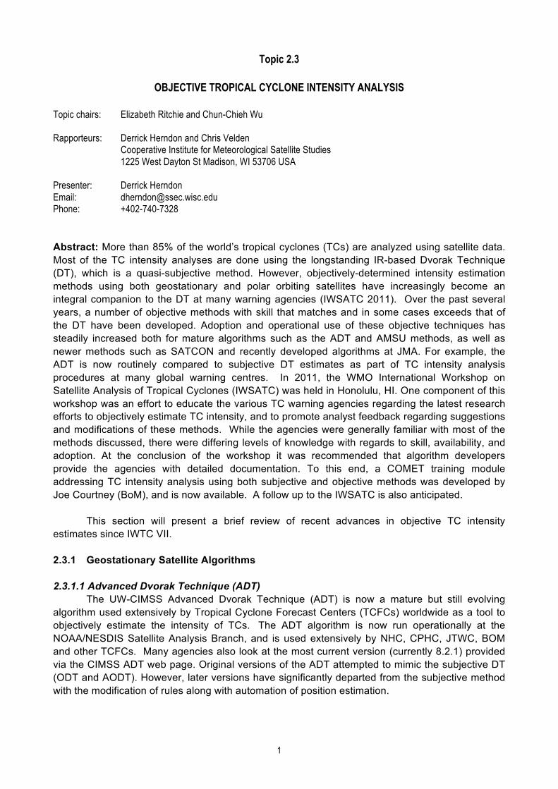
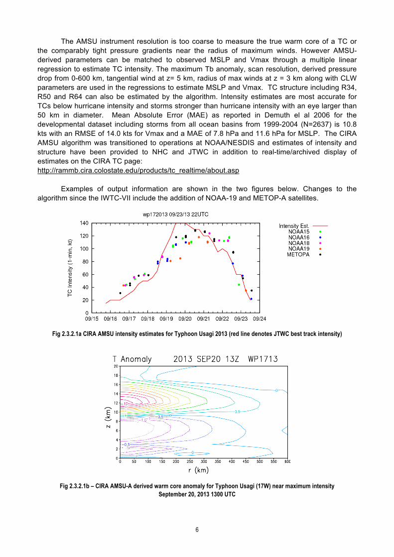
The AMSU instrument resolution is too coarse to measure the true warm core of a TC or the comparably tight pressure gradients near the radius of maximum winds. However AMSU-derived parameters can be matched to observed MSLP and Vmax through a multiple linear regression to estimate TC intensity. The maximum Tb anomaly, scan resolution, derived pressure drop from 0-600 km, tangential wind at z= 5 km, radius of max winds at z = 3 km along with CLW parameters are used in the regressions to estimate MSLP and Vmax. TC structure including R34, R50 and R64 can also be estimated by the algorithm. Intensity estimates are most accurate for TCs below hurricane intensity and storms stronger than hurricane intensity with an eye larger than 50 km in diameter. Mean Absolute Error (MAE) as reported in Demuth el al 2006 for the developmental dataset including storms from all ocean basins from 1999-2004 (N=2637) is 10.8 kts with an RMSE of 14.0 kts for Vmax and a MAE of 7.8 hPa and 11.6 hPa for MSLP. The CIRA AMSU algorithm was transitioned to operations at NOAA/NESDIS and estimates of intensity and structure have been provided to NHC and JTWC in addition to real-time/archived display of estimates on the CIRA TC page: http://rammb.cira.colostate.edu/products/tc_realtime/about.asp Examples of output information are shown in the two figures below. Changes to the algorithm since the IWTC-VII include the addition of NOAA-19 and METOP-A satellites.

Fig 2.3.2.1a CIRA AMSU intensity estimates for Typhoon Usagi 2013 (red line denotes JTWC best track intensity)

Fig 2.3.2.1b – CIRA AMSU-A derived warm core anomaly for Typhoon Usagi (17W) near maximum intensity

September 20, 2013 1300 UTC

7

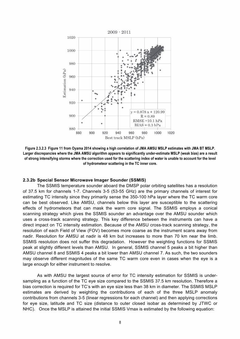
2.3.2.2 CIMSS AMSU algorithm The CIMSS AMSU intensity estimation algorithm uses AMSU-A channels 6-8 to derive Tb anomalies for each channel from limb-corrected AMSU data. Tb’s are then further corrected to account for hydrometeor scattering using a channel differencing approach that compares AMSU-A channels 2 and 15 to estimate what the Tb would be in the absence of scattering. A multiple regression approach is then used to estimate sea level pressure anomaly contributions from each channel. These individual channel contributions are then combined by weighting each pressure anomaly contribution using the hydrostatic assumption of that channel’s typical contribution based on the altitude of the channel. The final weighted pressure anomaly is then subtracted from estimates of environmental pressure provided by warning agencies to get estimated TC centre MSLP. Finally, corrections are applied to the MSLP estimate to account for under-sampling of the TC warm core as follows: - AMSU-B 89 GHz imagery is used to correct for true TC position offset relative to the AMSU- A FOV used for the estimate. Future updates will use the CIMSS ARCHER algorithm estimates of TC position for this correction. - Eye size information from the CIMSS ARCHER algorithm is used to correct for under- sampling that can result from the relatively coarse AMSU-A resolution. If a microwave eye size is not available from ARCHER then the eye size from the ADT is used. If neither of these sources is available the RMW estimate from the warning agency is used to get an eye size. - Small corrections are applied to account for estimate bias as a function of the TC location relative to the AMSU scan swath (near the edge of the swath or near nadir). AMSU intensity estimates are sent to NHC and JTWC through ATCF as well as other agencies as part of the CIMSS SATCON algorithm (section 2.3.4.2). Verification of AMSU estimates from 1999-2011 (N=852) in the Atlantic, Eastern Pacific and Western North Pacific for cases when aircraft data was available within three hours of the satellite pass resulted in a bias of 0.6 knots, MAE of 8.8 knots and RMSE of 11.4 knots. For MSLP the bias is 0.01 hPa, MAE of 5.3 hPa and RMSE of 7.2 hPa. Algorithm upgrades since IWTC-VII: 1) The loss of N-15 AMSU-B required that the AMSU–B 89 GHz correction used for this channel be replaced by a proxy. Currently this is done by comparing the difference between the scattering corrected AMSU-A channel 6 and the non-corrected Tb. 2) Weights applied to N-19 channel 8 were decreased due to increased noise in the channel. 2.3.2.3 JMA AMSU algorithm JMA began using an AMSU-based TC intensity estimation algorithm starting in 2013. AMSU-derived Tb anomalies in channels 6-8 are matched to a training sample consisting of 22 TCs in 2008 and validated against 57 TCs from 2009-2011. The algorithm computes the maximum anomaly from either of the three AMSU-A channels. Maximum Tbs are subtracted from an environmental Tb measured in an annulus between 550-600 km from the TC centre. Corrections are applied to account for random noise within the AMSU scan. A bias correction as a function of true TC position offset relative to the AMSU-A FOV location is applied to the Tb. Best Track (BT) estimates of TC position from JMA are used for this correction. Finally the scattering index of water (Grody 2001) is used to account for the presence of hydrometeors within the beam. After all corrections are applied, the corrected maximum Tb anomaly is used to estimate TC MSLP using linear regression (see figure 2.3.2.3 below). An evaluation of the algorithm’s skill was conducted by comparing estimates of MSLP for an independent sample of storms from 2009-2011 (N=1029) to BT estimates of MSLP from JMA, which consisted of primarily Dvorak estimates. Results of this comparison were a bias of 0.3 hPa and MAE of 10.1 hPa (Oyama 2014).

8

Figure 2.3.2.3 Figure 11 from Oyama 2014 showing a high correlation of JMA AMSU MSLP estimates with JMA BT MSLP. Larger discrepancies where the JMA AMSU algorithm appears to significantly under-estimate MSLP (weak bias) are a result of strong intensifying storms where the correction used for the scattering index of water is unable to account for the level

of hydrometeor scattering in the TC inner core. 2.3.2b Special Sensor Microwave Imager Sounder (SSMIS) The SSMIS temperature sounder aboard the DMSP polar orbiting satellites has a resolution of 37.5 km for channels 1-7. Channels 3-5 (53-55 GHz) are the primary channels of interest for estimating TC intensity since they primarily sense the 350-100 hPa layer where the TC warm core can be best observed. Like AMSU, channels below this layer are susceptible to the scattering effects of hydrometeors that can mask the warm core signal. The SSMIS employs a conical scanning strategy which gives the SSMIS sounder an advantage over the AMSU sounder which uses a cross-track scanning strategy. This key difference between the instruments can have a direct impact on TC intensity estimation. Because of the AMSU cross-track scanning strategy, the resolution of each Field of View (FOV) becomes more coarse as the instrument scans away from nadir. Resolution for AMSU at nadir is 48 km but increases to more than 70 km near the limb. SSMIS resolution does not suffer this degradation. However the weighting functions for SSMIS peak at slightly different levels than AMSU. In general, SSMIS channel 5 peaks a bit higher than AMSU channel 8 and SSMIS 4 peaks a bit lower than AMSU channel 7. As such, the two sounders may observe different magnitudes of the same TC warm core even in cases when the eye is a large enough for either instrument to resolve. As with AMSU the largest source of error for TC intensity estimation for SSMIS is under-sampling as a function of the TC eye size compared to the SSMIS 37.5 km resolution. Therefore a bias correction is required for TC’s with an eye size less than 38 km in diameter. The SSMIS MSLP estimates are derived by weighting the contributions of each of the three MSLP anomaly contributions from channels 3-5 (linear regressions for each channel) and then applying corrections for eye size, latitude and TC size (distance to outer closed isobar as determined by JTWC or NHC). Once the MSLP is attained the initial SSMIS Vmax is estimated by the following equation:

9

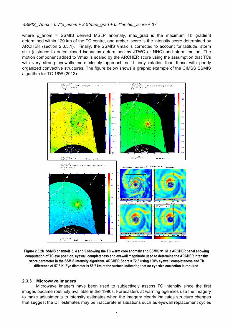
SSMIS_Vmax = 0.7*p_anom + 2.0*max_grad + 0.4*archer_score + 37 where p_anom = SSMIS derived MSLP anomaly, max_grad is the maximum Tb gradient determined within 120 km of the TC centre, and archer_score is the intensity score determined by ARCHER (section 2.3.3.1). Finally, the SSMIS Vmax is corrected to account for latitude, storm size (distance to outer closed isobar as determined by JTWC or NHC) and storm motion. The motion component added to Vmax is scaled by the ARCHER score using the assumption that TCs with very strong eyewalls more closely approach solid body rotation than those with poorly organized convective structures. The figure below shows a graphic example of the CIMSS SSMIS algorithm for TC 18W (2012).

Figure 2.3.2b SSMIS channels 3, 4 and 5 showing the TC warm core anomaly and SSMIS 91 GHz ARCHER panel showing computation of TC eye position, eyewall completeness and eyewall magnitude used to determine the ARCHER intensity

score parameter in the SSMIS intensity algorithm. ARCHER Score = 72.3 using 100% eyewall completeness and Tb difference of 57.3 K. Eye diameter is 56.7 km at the surface indicating that no eye size correction is required.

2.3.3 Microwave Imagers   Microwave imagers have been used to subjectively assess TC intensity since the first images became routinely available in the 1990s. Forecasters at warning agencies use the imagery to make adjustments to intensity estimates when the imagery clearly indicates structure changes that suggest the DT estimates may be inaccurate in situations such as eyewall replacement cycles

10

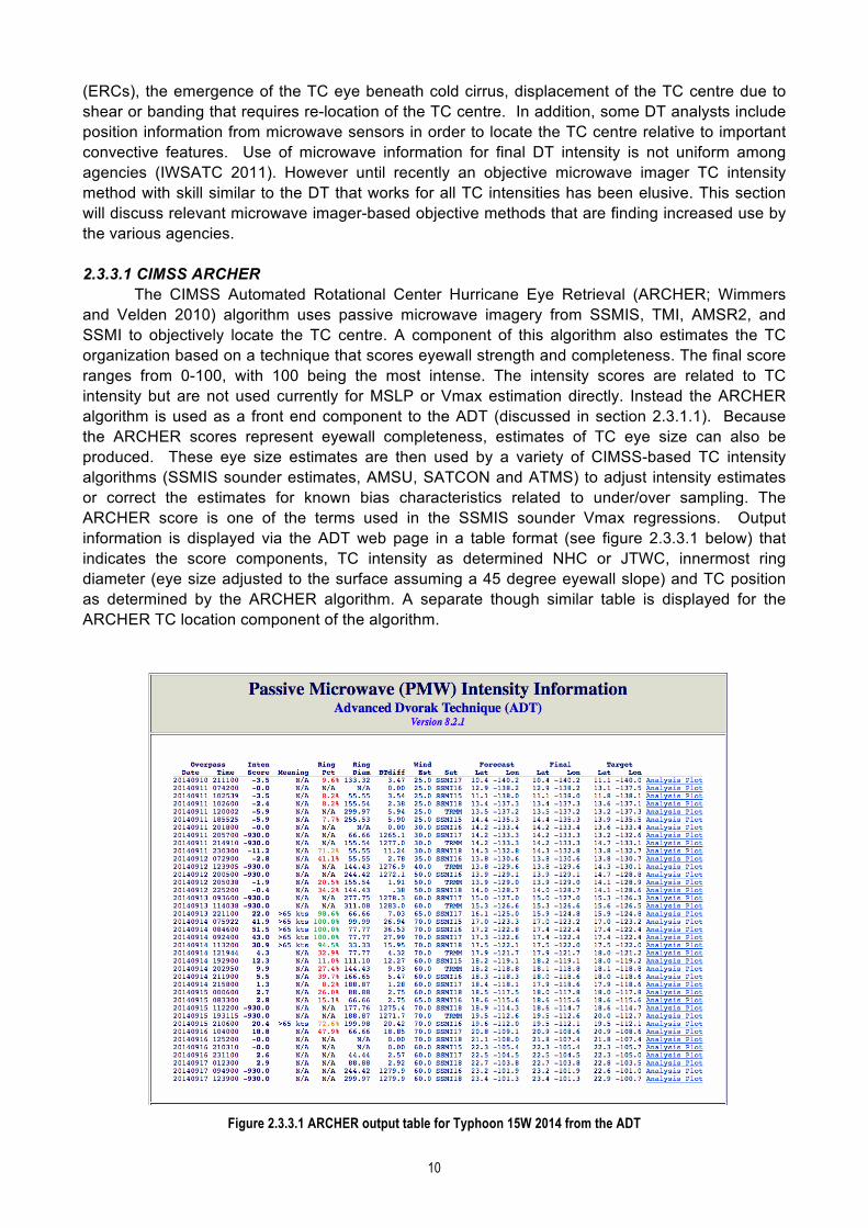
(ERCs), the emergence of the TC eye beneath cold cirrus, displacement of the TC centre due to shear or banding that requires re-location of the TC centre. In addition, some DT analysts include position information from microwave sensors in order to locate the TC centre relative to important convective features. Use of microwave information for final DT intensity is not uniform among agencies (IWSATC 2011). However until recently an objective microwave imager TC intensity method with skill similar to the DT that works for all TC intensities has been elusive. This section will discuss relevant microwave imager-based objective methods that are finding increased use by the various agencies. 2.3.3.1 CIMSS ARCHER The CIMSS Automated Rotational Center Hurricane Eye Retrieval (ARCHER; Wimmers and Velden 2010) algorithm uses passive microwave imagery from SSMIS, TMI, AMSR2, and SSMI to objectively locate the TC centre. A component of this algorithm also estimates the TC organization based on a technique that scores eyewall strength and completeness. The final score ranges from 0-100, with 100 being the most intense. The intensity scores are related to TC intensity but are not used currently for MSLP or Vmax estimation directly. Instead the ARCHER algorithm is used as a front end component to the ADT (discussed in section 2.3.1.1). Because the ARCHER scores represent eyewall completeness, estimates of TC eye size can also be produced. These eye size estimates are then used by a variety of CIMSS-based TC intensity algorithms (SSMIS sounder estimates, AMSU, SATCON and ATMS) to adjust intensity estimates or correct the estimates for known bias characteristics related to under/over sampling. The ARCHER score is one of the terms used in the SSMIS sounder Vmax regressions. Output information is displayed via the ADT web page in a table format (see figure 2.3.3.1 below) that indicates the score components, TC intensity as determined NHC or JTWC, innermost ring diameter (eye size adjusted to the surface assuming a 45 degree eyewall slope) and TC position as determined by the ARCHER algorithm. A separate though similar table is displayed for the ARCHER TC location component of the algorithm.

Figure 2.3.3.1 ARCHER output table for Typhoon 15W 2014 from the ADT

11

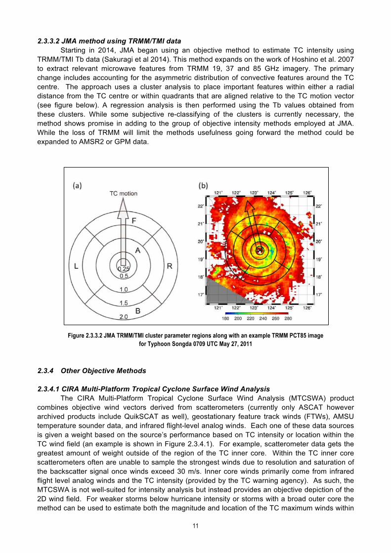
2.3.3.2 JMA method using TRMM/TMI data Starting in 2014, JMA began using an objective method to estimate TC intensity using TRMM/TMI Tb data (Sakuragi et al 2014). This method expands on the work of Hoshino et al. 2007 to extract relevant microwave features from TRMM 19, 37 and 85 GHz imagery. The primary change includes accounting for the asymmetric distribution of convective features around the TC centre. The approach uses a cluster analysis to place important features within either a radial distance from the TC centre or within quadrants that are aligned relative to the TC motion vector (see figure below). A regression analysis is then performed using the Tb values obtained from these clusters. While some subjective re-classifying of the clusters is currently necessary, the method shows promise in adding to the group of objective intensity methods employed at JMA. While the loss of TRMM will limit the methods usefulness going forward the method could be expanded to AMSR2 or GPM data.

Figure 2.3.3.2 JMA TRMM/TMI cluster parameter regions along with an example TRMM PCT85 image for Typhoon Songda 0709 UTC May 27, 2011

2.3.4 Other Objective Methods 2.3.4.1 CIRA Multi-Platform Tropical Cyclone Surface Wind Analysis The CIRA Multi-Platform Tropical Cyclone Surface Wind Analysis (MTCSWA) product combines objective wind vectors derived from scatterometers (currently only ASCAT however archived products include QuikSCAT as well), geostationary feature track winds (FTWs), AMSU temperature sounder data, and infrared flight-level analog winds. Each one of these data sources is given a weight based on the source’s performance based on TC intensity or location within the TC wind field (an example is shown in Figure 2.3.4.1). For example, scatterometer data gets the greatest amount of weight outside of the region of the TC inner core. Within the TC inner core scatterometers often are unable to sample the strongest winds due to resolution and saturation of the backscatter signal once winds exceed 30 m/s. Inner core winds primarily come from infrared flight level analog winds and the TC intensity (provided by the TC warning agency). As such, the MTCSWA is not well-suited for intensity analysis but instead provides an objective depiction of the 2D wind field. For weaker storms below hurricane intensity or storms with a broad outer core the method can be used to estimate both the magnitude and location of the TC maximum winds within

12

+/- 5 m/s. All data sources are adjusted to a level of 700 hPa and then the winds are reduced to surface winds using a correction factor of 0.9 for the winds within 100 km and then linearly decreasing to 0.75 out to 700 km. An assumption is made for the 0.9 factor that the TC contains vigorous convection within the inner core and thus some caution should be used for systems which are strongly sheared or have lost their convection near the inner core. Additional corrections are made to reduce over-land winds by 25%, and wind asymmetries associated with storm motion.

Figure 2.3.4.1 showing with CIRA MTCSWA weighting scheme for storms > 33 m/s (left) and an example 2D wind field product of Tropical Cyclone Faxai 2014 (right) demonstrating the ability to depict the asymmetric wind field associated with

the storm as the TC moved northeast at 6 m/s. The product provides a table indicating estimates of R34, R50, R64 and RMW.

2.3.4.2 CIMSS SATellite CONsensus Method (SATCON) Like the CIRA MTCSWA algorithm, the CIMSS SATCON algorithm combines information from multiple satellites and sensors. However, the focus of the SATCON algorithm is on producing TC intensity estimates in the form of maximum 1-min. sustained surface (10 meter) winds (Vmax). The algorithm currently uses information from the CIMSS ADT, CIRA and CIMSS AMSU and CIMSS SSMIS algorithms. Future versions will include estimates from the S-NPP ATMS sounder. Intensity estimates from the individual algorithms are combined into a single estimate by weighting each member according to the member’s past statistical performance. Statistical analysis over many years of evaluation reveals that each member algorithm has strengths and weaknesses that can be determined objectively in near real-time. For example, because the AMSU-A instrument uses a fairly coarse resolution, the sensor is unable to resolve the true warm core magnitude of the TC. While eye size inputs are used to correct for this under-sampling, statistics show that when the TC eye size is very small (i.e. less than 30 km in diameter) the AMSU RMSE tends to be higher for these TCs. ADT estimates tend to have lower RMSE for TCs with a well-defined eye in infrared imagery with higher RMSE for CDO and shear scenes. This information is used by SATCON to assign weights based on RMSE performance (statistical analysis typically done at the end of each TC season) for each algorithm. By weighting each algorithm independently, superior statistical performance is attained over a simple average of the estimates. Member weights for MSLP and Vmax from each algorithm are determined separately. Prior to weighting, some adjustments are made to the individual member estimates. For example, because the ADT currently does not adjust Vmax to account for storm motion (though storm motion is used as part of the Courtney-Knaff-Zehr pressure-wind relationship to get

13

MSLP), the climatological storm motion component of 6 knots is subtracted from the ADT-provided Vmax and the current TC motion component is added. Further TC structure information is added to SATCON by adding a 4th pseudo-member. Estimates of SATCON MSLP and the environmental pressure obtained from JTWC or NHC are used to get the TC pressure anomaly and along with ROCI, TC eye size, storm motion and latitude an estimate of Vmax is computed. The eye size correction adjusts the Vmax estimate for cases where the eye size deviates from the climatological value of ~ 46 km. Thus Vmax is increased for TCs with small eyes compared to climatology and decreased for large eyes. Only objective estimates of eye size from either infrared (ADT) or microwave (ARCHER) are used. One benefit of this correction is an adjustment of SATCON Vmax for TCs undergoing eyewall replacement cycles (ERCs). The P-W Vmax is combined with the member weighted Vmax using 0.25*SATCON_PW + 0.75* SATCON_members. Significant changes to SATCON since IWTC-VII include: - AMSU and SSMIS members are linearly interpolated to produce a continuous hourly estimate for each member. This results in a greater number of three-member/four-member SATCON estimate matches and reduces the estimate variability. - SATCON Vmax +/- 2 standard deviation lines have been added to plots for guidance diagnostics. - Storm age is used to correct for an early TC stage ‘too strong’ bias associated with AMSU and SSMIS estimates. The correction linearly goes to zero at 36 hours after initial TC bulletin.

Table 2.3.4.2a – SATCON Vmax performance (knots) compared to individual members 2006-2012. Validation is best track coincident with aircraft ground truth within 3 hours. AMSU and SSMIS are interpolated hourly to match the ADT.

N=1467 CIMSS AMSU CMISS ADT CIMSS SSMIS SATCON BIAS -1.0 0.2 -1.0 -0.9 MAE 9.8 9.3 8.2 6.9 RMSE 12.1 12.0 10.4 8.6

Table 2.3.4.2b – SATCON MSLP performance (hPa) compared to individual members 2006-2012. Validation is best track coincident with aircraft ground truth within 3 hours. AMSU and SSMIS are interpolated hourly to match the ADT.

N=1467 CIMSS AMSU CMISS ADT CIMSS SSMIS SATCON BIAS 0.7 3.4 1.4 0.6 MAE 4.6 9.0 5.9 4.2 RMSE 5.9 12.1 7.6 5.4

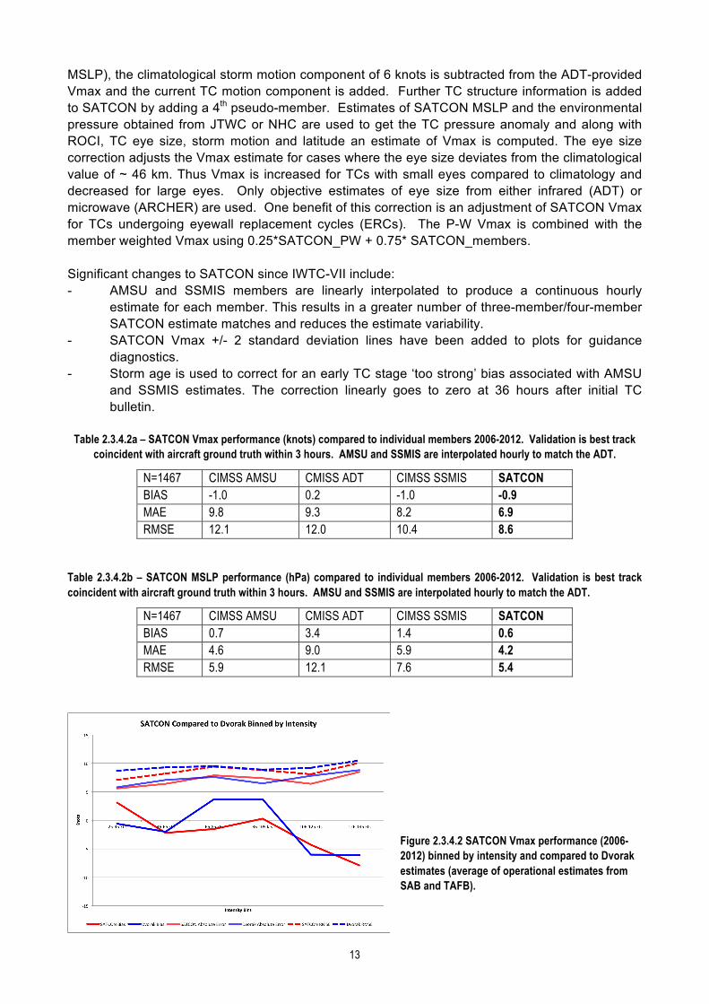
Figure 2.3.4.2 SATCON Vmax performance (2006-2012) binned by intensity and compared to Dvorak estimates (average of operational estimates from SAB and TAFB).  

14

Acknowledgements Special thanks to Kim Wood, Joe Courtney, Jeff Hawkins, Tsukasa Fujita, Thierry DuPont, Xiaoqin Lu and Hui Yu for their expert input on these topics. Acronyms used in the report ADT Advanced Dvorak Technique AMSU Advanced Sounding Unit ARCHER Automated Rotational Center Hurricane Eye Retrieval ATMS Advanced Temperature Microwave Sounder CIMSS Cooperative Institute for Meteorological Satellite Studies CIRA Cooperative Institute for Research in the Atmosphere CLOUD Cloud Grid Information Objective Dvorak Analysis DAV-T Deviation Angle Variance Technique DT Dvorak Technique (subjective) NHC National Hurricane Center JMA Japan Meteorological Agency JTWC Joint Typhoon Warning Center MSLP Minimum Sea Level Pressure SATCON SATellite CONsensus SAB Satellite Analysis Branch SSMIS Special Sensor Microwave Imager Sounder TAFB Tropical Analysis and Forecast Branch Vmax Maximum Sustained Wind References Burton, A, and C. Velden 2012: Proceedings of the International Workshop on Satellite Analysis of

Tropical Cyclones. WMO report No. TCP-52. Demuth, J, M. DeMaria and J. Knaff 2006: Improvement of the Advanced Microwave Sounding

Unit Tropical Cyclone Intensity and Size Estimation Algorithms. J. Appl. Meteor and Clim, 45, 1573-1581.

Knaff, J, M. DeMaria, D. Molenar, C. Sampson, M. Seybold 2011: An Automated, Objective, Multi-Satellite-Platform Topical Cyclone Surface Wind Analysis. J. Appl Meteor and Clim, 50, 2149-2166.

Hawkins, J. and C. Velden, 2011: Supporting Meteorological Field Experiment Missions and Post-mission Analysis with Satellite Digital Data and Products. Bulletin of the American Meteorological Society, 92, 1009-1022.

Herndon, D. C., C. S. Velden, K. Brueske, R. Wacker, and B. Kabat, 2004: Upgrades to the UW-CIMSS AMSU-based tropical cyclone intensity algorithm. Preprints, 26th Conf. on Hurricanes and Tropical Meteorology, Miami, FL, Amer. Meteor. Soc., 4D.1.

(http://ams.confex.com/ams/26HURR/techprogram/paper_75933.htm) Herndon, D. C., C. S. Velden, 2012: Update on SATellite-based CONsensus Approach to TC

Intensity Estimation. Preprints, 30th Conf. on Hurricanes and Tropical Meteorology, Ponte Vedra, FL, Amer. Meteor. Soc., 7C.2.

Kishimoto, .K, M. Sasaki and M. Kunitsugu, 2013: Cloud grid information objective Dvorak analysis (CLOUD) at the RSMC Tokyo - Typhoon Center. RSMC Tokyo-Typhoon Center Technical Review, No. 15. (http://www.jma.go.jp/jma/jma-eng/jma-center/rsmc-hp-pub-eg/techrev.htm)

15

Olander, T. L., and C. S. Velden, 2007: The advanced Dvorak technique: Continued development of an objective scheme to estimate tropical cyclone intensity using geostationary infrared satellite imagery. Wea. Forecasting, 22, 287–299.

Oyama, R, 2014: Estimation of tropical cyclone central pressure from warm core intensity observed by the Advanced Microwave Sounding Unit-A (AMSU-A). Pap. Meteor. Geophys., 65, 35-56. (https://www.jstage.jst.go.jp/article/mripapers/65/0/65_35/_article)

Piñeros, M. F., E. A. Ritchie, and J. S. Tyo, 2008: Objective measures of tropical cyclone structure and intensity change from remotely sensed infrared image data. IEEE Transactions on Geoscience and Remote Sensing, 46, 3574-3580.

Piñeros, M. F., E. A. Ritchie, and J. S. Tyo, 2011: Estimating tropical cyclone intensity from infrared image data. Wea. Forecasting, 26, 690-698.

Ritchie, E. A., G. Valliere-Kelley, M. F. Piñeros, and J. S. Tyo, 2012: Tropical cyclone intensity estimation in the North Atlantic using an improved deviation angle variance technique. Wea. Forecasting, 27, 1264–1277.

Ritchie, E. A., K. M. Wood, O. G. Rodríguez-Herrera, M. F. Piñeros, and J. S. Tyo, 2014: Satellite-derived tropical cyclone intensity in the North Pacific Ocean using the deviation-angle variance technique. Wea. Forecasting, 29, 505–516.

Sakuragi, T., S. Hoshino, and N. Kitabatake, 2014: Development and verification of a tropical cyclone intensity estimation method reflecting the variety of TRMM/TMI brightness temperature distribution. RSMC Tokyo-Typhoon Center Technical Review, No. 16. (http://www.jma.go.jp/jma/jmaeng/jma-center/rsmc-hp-pub-eg/techrev.htm)

Wimmers, A., and C. Velden, 2010: Objectively Determining the Rotational Center of Tropical Cyclones in Passive Microwave Satellite Imagery. J. Appl. Meteor and Clim. 49, 2013-2034.

Xiaoqin L., H. Yu, 2013: An Objective Tropical Cyclone Intensity Estimation Model Based on Digital IR Satellite Images. Tropical Cyclone Research and Review. 2(4), 53-62

______