Environmental Control of Tropical Cyclone Intensity

1 APRIL 2004 843E M A N U E L E T A L .

q 2004 American Meteorological Society

Environmental Control of Tropical Cyclone Intensity

KERRY EMANUEL, CHRISTOPHER DESAUTELS, CHRISTOPHER HOLLOWAY, AND ROBERT KORTY

Program in Atmospheres, Oceans, and Climate, Massachusetts Institute of Technology, Cambridge, Massachusetts

(Manuscript received 7 April 2003, in final form 5 November 2003)

ABSTRACT

The influence of various environmental factors on tropical cyclone intensity is explored using a simple coupledocean–atmosphere model. It is first demonstrated that this model is capable of accurately replicating the intensityevolution of storms that move over oceans whose upper thermal structure is not far from monthly mean cli-matology and that are relatively unaffected by environmental wind shear. A parameterization of the effects ofenvironmental wind shear is then developed and shown to work reasonably well in several cases for which themagnitude of the shear is relatively well known. When used for real-time forecasting guidance, the model isshown to perform better than other existing numerical models while being competitive with statistical methods.In the context of a limited number of case studies, the model is used to explore the sensitivity of storm intensityto its initialization and to a number of environmental factors, including potential intensity, storm track, windshear, upper-ocean thermal structure, bathymetry, and land surface characteristics. All of these factors are shownto influence storm intensity, with their relative contributions varying greatly in space and time. It is argued that,in most cases, the greatest source of uncertainty in forecasts of storm intensity is uncertainty in forecast valuesof the environmental wind shear, the presence of which also reduces the inherent predictability of storm intensity.

1. Introduction

Forecasts of hurricane movement have improvedsteadily over the last three decades owing to a combi-nation of better observations and much improved nu-merical models (DeMaria and Kaplan 1997). By con-trast, there has been comparatively little advance in pre-dictions of intensity (as measured, e.g., by maximumsurface wind speed) in spite of the application of so-phisticated numerical models (DeMaria and Kaplan1997). The best intensity forecasts today are statisticallybased (DeMaria and Kaplan 1994). While there is muchhope that three-dimensional coupled models will leadto better understanding of the factors that control hur-ricane intensity and to increased skill of hurricane in-tensity forecasts (Bender and Ginis 2000), at presentmodels do not have enough horizontal resolution to cap-ture the full magnitude of intense storms. Experimentswith research-quality three-dimensional numerical mod-els show nontrivial dependence of model storm intensityon horizontal resolution even at grid spacings as smallas 1–2 km (Shuyi Chen 2002, personal communication).Fortunately, it is probably not necessary to capture fullstorm intensity in order to achieve good track forecasts.

Changes in tropical cyclone intensity may be looselypartitioned between changes arising from changing con-ditions of the storm’s environment and internal fluctu-

Corresponding author address: Kerry Emanuel, MIT, Room 54-1620, 77 Massachusetts Ave., Cambridge, MA 02139.E-mail: [email protected]

ations that may reflect storm-scale instabilities or thestochastic effects of high-frequency transients such asmoist convection. Concentric eyewall cycles are knownto be associated with sometimes dramatic changes instorm intensity (Willoughby and Black 1996), althoughit is not yet clear whether these are manifestations ofstrictly internal instabilities or are triggered and/or con-trolled by the large-scale environment. Work by Moli-nari and Vollaro (1989, 1990) and Nong and Emanuel(2003) suggests that eyewall cycles may be triggeredby environmental influences but, once initiated, developautonomously. Owing to the relatively short time scalesof phenomena like these, their dominance in tropicalcyclone intensity change would compromise predict-ability on such time scales. We here take as our workingpremise that internal fluctuations are generally of sec-ondary importance in tropical cyclone intensity change.We test this premise by attempting to predict intensitychange using a model whose behavior is largely con-trolled by external environmental factors.

The majority of the research literature on hurricaneintensity focuses on the prestorm thermodynamic en-vironment (e.g., Emanuel 1986, 1988; Bister and Eman-uel 1998), and certain properties of the atmospheric en-vironment, such as the vertical shear of the horizontalwind (e.g., Jones 2000; Frank and Ritchie 2001), anddynamical features, such as disturbances in the uppertroposphere (e.g., Molinari and Vollaro 1989, 1990,1995). This remains so even though it is well knownthat hurricanes alter the surface temperature of the ocean

844 VOLUME 61J O U R N A L O F T H E A T M O S P H E R I C S C I E N C E S

over which they pass (Price 1981) and that a mere 2.5-K decrease in ocean surface temperature near the coreof the storm would suffice to shut down energy pro-duction entirely (Gallacher et al. 1989). Simulationswith three-dimensional coupled atmosphere–oceanmodels (Gallacher et al. 1989; Khain and Ginis 1991;Schade and Emanuel 1999) confirm that interaction withthe ocean is a strong negative feedback on storm inten-sity.

The weight given in the literature to strictly atmo-spheric environmental factors reflects a poor collectiveunderstanding of the relative importance of the variousprocesses to which tropical cyclone intensity change hasbeen ascribed. The best statistical prediction schemesaccount for prestorm sea surface temperature and ver-tical wind shear but do not account for feedback fromocean interaction.

In this paper, we employ a simple but skillful coupledatmosphere–ocean tropical cyclone model to explore thesensitivity of tropical cyclone intensity to various en-vironmental factors. The atmospheric model is phrasedin potential radius coordinates, permitting exceptionallyhigh horizontal resolution in the eyewall, where it isneeded, at low computational cost. This model is cou-pled to a simple one-dimensional ocean model, whichhas been shown to mimic almost perfectly the feedbackeffect of a fully three-dimensional ocean model. We firstdemonstrate that this coupled model is capable of ac-curately simulating the intensity evolution of storms thatmove over an ocean whose upper thermal structure isclose to climatology and that are unmolested by verticalshear of the environmental wind. We then develop anempirical parameterization of the effects of wind shear,using data from a few storms for which the environ-mental shear is relatively well known, and show thatthis parameterization is effective in several cases forwhich shear was the dominant factor inhibiting stormintensity. Finally, the coupled model is used to explorethe effects of various environmental factors in control-ling the intensity evolution of a limited number of eventsselected to illustrate these factors.

2. Model design

a. Atmospheric model

The atmospheric model is described in detail byEmanuel (1995a). It is constructed on the assumptionthat the storm is axisymmetric, that the airflow is inhydrostatic and gradient wind balance, and that the vor-tex is always close to a state of neutral stability to slant-wise convection in which the temperature lapse rate iseverywhere and always assumed to be moist adiabaticalong angular momentum surfaces. Thus, the saturatedmoist potential vorticity is zero everywhere, and thebalance conditions allow this quantity to be inverted,subject to certain boundary conditions (Shutts 1981;Emanuel 1986). These constraints place strong restric-

tions on the structure of the vortex so that, with theexception of the water vapor distribution, the verticalstructure is determined by the radial distribution ofboundary layer moist entropy and by the vorticity at thetropopause. The water vapor distribution is character-ized by the moist entropy of the boundary layer and ofa single layer in the middle troposphere.

Moist convection is represented by one-dimensionalupdraft and downdraft plumes, whose mass flux is de-termined to insure approximate entropy equilibrium ofthe boundary layer (Raymond 1995) and for which theprecipitation efficiency is taken to be a function of theenvironmental relative humidity in the middle tropo-sphere. The saturation moist entropy above the bound-ary layer (and along angular momentum surfaces) close-ly follows the boundary layer moist entropy in regionsof convection but is determined by large-scale subsi-dence and radiative cooling in regions, such as the eye,that are stable to moist convection.

The model variables are phrased in ‘‘potential radius’’coordinates (Schubert and Hack 1983). Potential radius(R) is proportional to the square root of the absoluteangular momentum per unit mass about the storm centerand is defined by

2 2fR 5 2rV 1 f r , (1)

where r is the physical radius, V is the azimuthal ve-locity, and f is the Coriolis parameter. In the runs pre-sented here, there are 50 nodes that span 1000 km, giv-ing an average resolution of 20 km; however, the res-olution is substantially finer than this in regions of highvorticity, such as the eyewall, and can be as fine as 1–2 km in the eyewalls of intense storms.

When run with a fixed sea surface temperature anda fixed atmospheric environment, the steady-state stormintensity is controlled strictly by the potential intensity,which is a function of sea surface temperature, storm-top environmental temperature, and air–sea thermody-namic disequilibrium alone. The potential intensity isthe maximum steady intensity a storm can achieve basedon its energy cycle, in which the heat input by evapo-ration from the ocean and from dissipative heating, mul-tiplied by a thermodynamic efficiency, is balanced bymechanical dissipation in the storm’s atmosphericboundary layer (Bister and Emanuel 1998). We stressthat the steady-state intensity behavior in this model iscontrolled only by the potential intensity; the particularcombination of sea surface and outflow temperaturesand air–sea disequilibrium is immaterial.

One potentially important source of uncertainty is theformulation of the surface fluxes of enthalpy and mo-mentum to which the evolution of storm intensity issensitive (Emanuel 1995b). The model uses classicalbulk aerodynamic flux formulas based on the near-sur-face gradient wind speed. After some experimentation,we found that good simulations are obtained using en-thalpy and momentum transfer coefficients that areequal to each other and increase linearly with gradient


FIG. 1. Assumed (left) kinematic and (right) thermal structure ofthe upper ocean. The horizontal velocity u and temperature T areassumed to be homogeneous in a mixed layer of thickness h. Thereis a prescribed jump in temperature, DT, across the base of the mixedlayer below which the velocity is assumed to vanish and temperatureis assumed to decrease linearly with depth.

wind speed. While this functional dependence of theenthalpy transfer coefficient on wind is not supportedby observations at low wind speed (Large and Pond1982), recent experiments with a laboratory apparatusshow that this coefficient does indeed increase with windspeed once the latter exceeds about 15 m s21 (Alamaroet al. 2002).

To forecast real events, this atmospheric model ismodified in several ways. First, the potential intensityis allowed to vary in time during the integration to re-flect variations in potential intensity along the past andforecast track of the storm. (The potential intensity isheld fixed across the spatial domain of the model, how-ever.) Second, the sea surface temperature is allowed tovary with time and radius to reflect coupling to the one-dimensional ocean model described in section 2b. Fi-nally, a landfall algorithm is added in which the coef-ficient of surface enthalpy flux is assumed to vary lin-early from unity to zero as the elevation of the coastalplain increases from 0 to 40 m. This procedure is dis-cussed in section 5f.

One advantage of this model is its computationalspeed: a typical storm can be simulated in less than aminute on a typical desktop computer. It arguably con-tains all the essential axisymmetric physics necessaryfor tropical cyclone simulation, only neglecting any de-partures of the temperature profile from moist adiabaticon angular momentum surfaces and representing thevertical structure of relative humidity by only two layersin the troposphere. Aside from these approximations,the main limitation of the model is its axisymmetrywhich, among other problems, precludes any direct in-fluence from environmental wind shear, which is knownto be a major factor inhibiting tropical cyclone inten-sification; indeed, statistical analyses show that windshear is one of the primary predictors of storm intensitychange (DeMaria and Kaplan 1994). Based on experi-ence with the coupled model, we have developed a pa-rameterization of shear effects; this is described in sec-tion 5c.

b. Ocean model

The axisymmetric hurricane model is coupled to theone-dimensional ocean model developed by Schade(1997). In this model, the mixed layer depth is calculatedbased on the assumed constancy of a bulk Richardsonnumber, while the mixed layer momentum is driven bysurface stress and entrainment. Horizontal advection andthe Coriolis acceleration are omitted.

The upper-ocean horizontal velocity and temperatureare assumed to have the vertical structure illustrated inFig. 1 with finite jumps of velocity and buoyancy acrossthe base of the mixed layer. Ignoring horizontal advec-tion and Coriolis accelerations, the time rate of changeof the vertically averaged horizontal momentum of theupper ocean is given by

]rhu5 |t |, (2)s]t

where r is the density of seawater, h is the mixed layerdepth (see Fig. 1), u is the magnitude of the mixed layervelocity, and ts is the vector wind stress, obtained fromthe atmospheric model. While (2) describes the changesin mixed layer momentum experienced by an ocean col-umn fixed in space, the atmospheric model requiresocean temperature at its nodes in potential radius co-ordinates. For ocean columns ahead of the storm, thetransformation of (2) into the atmospheric model’s po-tential radius space gives

]rhu ]r ]R ]ruh5 |t | 1 u 1 , (3)s t1 2]t ]t ]r ]R

where ut is the translation speed of the storm, the no-tation ]/]t denotes a partial derivative in time at fixedpotential radius, and the quantities ]r/]t and ]R/]r arededuced from the atmospheric model.

We assume that vertical mixing is the only importanteffect on temperature during the passage of a tropicalcyclone and ignore horizontal advection and surfaceheat exchange. Price (1981) demonstrates that surfacetemperature change is usually dominated by mixing,with cooling by surface fluxes a secondary factor. Underthese conditions, the vertically integrated enthalpy re-mains constant:

0 0

rC T dz 5 rC T dz, (4)E l E l i

2` 2`

where Cl is the heat capacity of seawater, T is its tem-perature, and Ti is the initial temperature. In evaluatingthe integrals in (4), we approximate Cl and r as constantsand, as illustrated in Fig. 1, we assume that the tem-perature lapse rate below the mixed layer is constant.The initial state of the ocean is described using onlyfour quantities: surface temperature, mixed layer depth,the temperature jump DTi at the base of the mixed layer,


FIG. 2. Configuration of the ocean model. One-dimensional col-umns are strung out along the future path of the storm at the loci ofthe intersections of the atmospheric model’s potential radius surfaceswith the storm track. In a coordinate system moving with the stormcenter, properties are advected from one ocean column to the nextradially inward along the storm track.

and the temperature lapse rate G below the mixed layer.The initial mixed layer velocity u is assumed to be zero.

Entrainment into the mixed layer is modeled by as-suming that the bulk Richardson number of the mixedlayer remains constant (Price 1981). This Richardsonnumber is defined

gDshR [ ,

2su

where g is the acceleration of gravity, s is the potentialdensity, and Ds is its jump across the base of the mixedlayer. We here ignore pressure and salinity effects onpotential density and approximate the bulk Richardsonnumber as

gaDThR . 5 R 5 1.0, (5)crit2u

where a is the coefficient of thermal expansion of sea-water, which we approximate by a constant represen-tative of the tropical upper ocean. In this model, werequire R to be equal to a critical value, which we heretake to be 1.

Thus, our simplified ocean model consists of (3)–(5).The momentum equation (3) is integrated forward intime, with the surface stress supplied by the atmosphericmodel. The mixed layer depth h and temperature jumpDT are then diagnosed using (4) and (5) together withthe assumed vertical structure illustrated in Fig. 1.

c. Atmosphere–ocean coupling

In coupling the atmosphere and ocean models it isassumed that a hurricane responds principally to seasurface temperature changes under its eyewall and thatthese can be closely approximated by sea surface tem-perature changes under that part of the eyewall that liesalong the storm track. Thus, as illustrated in Fig. 2, theocean response is modeled by a set of one-dimensionalocean columns along the storm track. The sea surfacetemperature value used by the axisymmetric model is asimple average of the values ahead of and behind thestorm at the radius in question. Also, to save compu-tational time, only the columns ahead of and at the centerof the storm are calculated and the storm-center seasurface temperature anomaly is used to represent con-ditions throughout the eye and under the eyewall. Whilethis approximation misses the wake of the storm, whereinertial oscillations have a strong influence on mixing(Price 1981), the model cyclone responds most stronglyto sea surface temperature anomalies directly under itseyewall and is hardly influenced by temperature anom-alies outside its core.

We tested this coupling formulation by comparingsimulations based on it with those using the same at-mospheric model coupled to the three-dimensionalocean model of Cooper and Thompson (1989), as de-scribed in Schade and Emanuel (1999). In those sim-

ulations, the ocean model was integrated on a regulargrid, and the sea surface temperature was interpolatedinto the potential radius coordinate of the atmosphericmodel and averaged in azimuth about the storm center.The Cooper–Thompson model is discretized into fourlayers, but uses the same entrainment closure as thecolumn model used here.

In this test, the tropical cyclone is assumed to betranslating in a straight line at a constant speed of 7 ms21 over an ocean with an unperturbed mixed layer depthof 30 m. Figure 3 compares the maximum surface windspeed evolution of three simulations: an uncoupled sim-ulation in which the sea surface temperature is heldfixed, a ‘‘full physics’’ simulation in which the completeocean model is integrated and the surface temperatureused by the atmospheric model is averaged in azimutharound the storm center, and a run using the simplifiedmodel described above in which the ocean model isintegrated only along the path taken by the center ofthe storm and the sea surface temperatures ahead of andunder the eye are used by the atmospheric model. Thesimplified model does surprisingly well, producing re-sults that are indistinguishable from the simulation usingthe full ocean model. At translation velocities less thanabout 4 m s21, however, the simplified model overes-timates the ocean feedback effect and thereby under-estimates the maximum wind speed by about 10%.

This comparison demonstrates that vertical turbulentmixing so dominates the physics of sea surface tem-perature change that all other processes may be ne-glected during the time between the onset of strongwinds and the passage of the eye. While strong verticalmixing is also induced by inertial oscillations excitedby the storm, they primarily affect sea surface temper-


FIG. 3. Evolution with time of the maximum surface wind speedin three different integrations of the coupled atmosphere–ocean mod-el. In each case, the storm is translating uniformly at 7 m s21 overa horizontally homogeneous ocean with an unperturbed mixed layerdepth of 30 m. The solid curve shows the results of a simulationcoupling the atmospheric model to a three-dimensional ocean model;the dashed line shows the results of a reference run with fixed seasurface temperature, and the dotted curve shows the results of in-tegrating a string of one-dimensional columns along the storm track.In this case, the full physics simulation and the simulation using thestring model are very nearly indistinguishable.

atures well to the rear of the storm center, and thesehave little effect on storm intensity. Indeed, to a goodapproximation, our atmospheric model is sensitive tosurface conditions only under the storm’s eyewall.

We have performed several experiments comparingthe full physics and simplified formulations for a varietyof initial conditions and translations speeds. These showthat the simplified model usually performs quite well.The largest differences between simulations using thefull and simplified physics occur for very slow trans-lations speeds (,3 m s21), when neglected processes,such as Ekman pumping, are comparatively important.

3. Data and initialization

In the simulations of real events described presently,the coupled model is supplied with an observed and/orforecast storm track and with information about theprestorm potential intensity, ocean mixed layer depth,submixed layer ocean thermal stratification, and ba-thymetry/topography along the storm track. In some ofthe cases presented below, we also supply an estimateof the environmental wind shear along the storm track,used in the formulation described in section 5c. Themodel is initialized using a synthetic warm-core vortex.In each of the cases discussed below, the geometry ofthe vortex and the value of the Coriolis parameter arefixed at prescribed values, though in principle they canbe varied according to the size and latitude of the realsystem. The maximum wind speed of this initial vortexis specified to be the ‘‘best-track’’ estimated wind speed

at the beginning of the storm’s life.1 Given the balancecondition of the model, this also effectively initializesthe mass (temperature) distribution. On the other hand,the water vapor distribution is not initialized by thisprocedure, and observations of moisture are generallyinsufficient for this purpose. But the initial intensifi-cation of the storm proves quite sensitive to the initialwater vapor distribution, and we make use of this sen-sitivity to initialize the water vapor (actually, the middlelevel entropy) based on observations of the rate ofchange of storm intensity. To accomplish this, the evo-lution of the model storm’s intensity is at each time stepadjusted toward that of the estimated intensity over afixed interval of time by varying the rate at which lowentropy air is injected into the storm’s core in the middletroposphere. That is, to the model’s middle-layer moistentropy equation (see Emanuel 1995a) is added an extraterm:

]xm 5 · · · 1 g(V 2 V )(x 2 x ), (6)obs sim m m0]t

where xm is the middle-level moist entropy variable, xm0

its unperturbed ambient value, the ellipses represent theother terms in the entropy equation, g is a constantnumerical coefficient, Vobs is the best-track maximumwind speed, and Vsim is the maximum wind speed in thesimulation (with a fraction of the translation speed add-ed back; see footnote 1). The effect of this added termis to adjust the entropy of the middle levels of the stormupward or downward in proportion to the differencebetween the simulated and observed intensity; this inturn drives the storm intensity toward the observationalestimate. This procedure insures that the simulatedstorm is dynamically and thermodynamically self-con-sistent by demanding consistency with both the ob-served maximum wind speed and the observed rate ofintensity change. The adjustment is implemented duringa prescribed interval (usually 1–2 days) for hindcastevents and during the whole period up to the currenttime for real-time forecasts. After the period of adjust-ment (hereafter, the ‘‘matching interval’’), the modelintensity evolves freely.

For real-time intensity forecasts, the past and pre-dicted storm positions and intensities are taken fromofficial forecasts provided by the National Oceanic andAtmospheric Administration (NOAA) National Hurri-cane Center (NHC) for Atlantic and eastern Pacificstorms and by the U.S. Navy’s Joint Typhoon WarningCenter (JTWC) for all other events. When run in ‘‘hind-

1 To account for the contribution of the storm’s translation speedto the maximum wind speed, we subtract a specified fraction of theformer from the latter, to obtain the purely circular component of themaximum wind speed. Experience has shown that subtracting the fulltranslation speed from the reported maximum wind speed often resultsin a system that is too weak. Here we take the specified fraction tobe 0.4. In subsequent comparisons of model and observed wind speed,this contribution from the translation speed is added back to the modeloutput.


cast’’ mode, the model uses best-track data supplied bythe two aforementioned centers, except where otherwisestated. Positions and intensities recorded or predictedevery 6 hours are linearly interpolated in time to themodel’s time step. It should be borne in mind that notall of the reported wind speeds are directly measuredby aircraft or radar; some are partially subjective esti-mates based on satellite imagery.

The potential intensity in the Tropics is observed tovary only slowly in time, being governed mostly by seasurface temperature. Therefore, for real-time forecasts,the model’s potential intensity is taken from data re-corded at the beginning of the storm’s life.2

To calculate potential intensity, we use sea surfacetemperature and atmospheric temperature analyses on a18 latitude–longitude grid supplied from the NationalCenters for Environmental Prediction (NCEP), recordedat 0000 UTC near the beginning of the storm’s life. Thesea surface temperatures used in these analyses are up-dated weekly, but we do not update them during the lifeof the storm because storm-induced SST anomalies oc-casionally affect the analyzed SSTs. Including these inthe potential intensity used by the model would resultin double counting of the SST feedback since the modelproduces its own storm-induced anomalies. The poten-tial intensity is calculated from an algorithm describedin Bister and Emanuel (2002) and is supplied daily bythe Center for Land–Atmosphere Prediction (COLA;maps of potential intensity, generated by COLA, areavailable online at http://grads.iges.org/pix/hurpot.html).For hindcast events, however, we use monthly meanclimatological potential intensities. These were calcu-lated using NCEP–National Center for Atmospheric Re-search (NCAR) monthly mean reanalysis data (Kalnayet al. 1996) from the years 1982–95, inclusive, as de-scribed in Bister and Emanuel (2002). The same poten-tial intensity algorithm was used as for the real-timepotential intensities. The effects of using monthly meanpotential intensity instead of actual potential intensityare explored in section 5e.

The initial state of the ocean along the storm track isdescribed by only two parameters: the ocean mixed layerdepth and the temperature gradient just beneath themixed layer. (We take the initial temperature jump atthe base of the mixed layer, DT1, to have the prescribedvalue of 0.5 K.) Lacking real-time ocean analyses, weare forced to rely on monthly mean climatology and forthis use 18 gridded data from Levitus (1982). (In section5d we attempt to use sea surface altimetric measure-ments to modify this mixed layer depth climatology.)Both quantities are linearly interpolated in space to thebest track or forecast storm position and in time to the

2 An important motive for not updating the potential intensity isthe desire to avoid using analyzed potential intensity that may reflectthe presence of the storm in question. The analyzed storm’s warmcore reduces the analyzed potential intensity that, on the other hand,is supposed to reflect undisturbed environmental conditions.

actual date, assigning the monthly mean climatology tothe 15th day of each month.

Bathymetry and topography are specified to ¼8 res-olution and linearly interpolated to the storm positions.This is used to detect landfall and, also, to reveal placeswhere the ocean mixed layer extends to the sea floor sothat surface cooling by mixing cannot occur. As de-scribed in section 2a, the landfall algorithm is one ofmaximum simplicity: The coefficient of surface enthal-py flux decreases linearly with land elevation at thestorm center, vanishing over terrain higher than 40 m.

Unless otherwise stated, estimates of the verticalshear of the environmental wind, used in our parame-terization of shear effects (section 5c), are those usedas real-time input to the Statistical Hurricane IntensityPrediction Scheme (SHIPS), described in DeMaria andKaplan (1994). These estimates are made by smoothingthe spatial distribution of analyzed and forecasted valuesof the 850–200-hPa horizontal winds so as to removeas much as possible of the shear associated directly withthe storm circulation. We make no assertion that the850–200-hPa wind shear is the optimal quantity to use;it is merely expedient to use these values until and unlesssuperior measures are developed.

In each of the cases presented below, the evolutionof maximum surface wind speed in the model is com-pared to the observed evolution; no attempt has beenmade to compare the evolutions of model and observedstorm structure or precipitation rates.

4. Model performance

The model, named the Coupled Hurricane IntensityPrediction System (CHIPS) for brevity, has been runexperimentally at both NHC and JTWC since 2000. Be-ginning in the 2001 Atlantic season and in September2002 in the North Pacific, a parameterization of sheareffects (described in section 5c) has been included inthe forecast model. This parameterization has been suc-cessively refined over the last two seasons. Forecast skillhas so far been evaluated for Atlantic storms only. Theroot-mean-square intensity errors of the CHIPS fore-casts are comparable to the best statistical forecasts(SHIPS) and smaller than the best deterministic modelguidance (Geophysical Fluid Dynamics Laboratory,GFDL). Figure 4 shows results for the 2002 Atlantichurricane season as an example.

5. Sensitivity to environment and initialization

In this section we illustrate the sensitivity of the cou-pled model to initial conditions and to various environ-mental factors. We focus on a limited number of cases,beginning with a single case of a storm that developedand decayed over the central tropical North Atlantic, inwhich there was virtually no shear and little evidenceof significant prestorm upper-ocean thermal anomalies.


FIG. 4. Root-mean-square intensity errors (kt) for the 2002 Atlantichurricane season for SHIPS (solid), GFDL hurricane model (dashed),and CHIPS (dotted) forecasts as a function of forecast lead time.

FIG. 5. Evolution of maximum wind speed in Hurricane Gert, 1999.(a) Best track (solid) is compared to CHIPS hindcast (dashed). Solidblack bar at bottom left shows initialization interval in which themodel is matched to observations. (b) As in (a) but without oceancoupling.

a. The importance of ocean interaction

Hurricane Gert is a good example of model stormbehavior when environmental shear is small. Gert de-veloped west of the Cape Verde Islands in mid Septem-ber 1999 and, after moving west-northwestward for 5days, turned northward over the central North Atlantic.Figure 5a shows the evolution of the best-track intensitytogether with a model hindcast. (Real-time forecasts ofthis system were skillful.) There is good agreement be-tween the observed and predicted intensity. The controlforecast is compared in Fig. 5b to another simulationin which ocean feedback is omitted. Forecast errors ow-ing to omission of ocean feedback reach values as largeas 25 m s21 on 18 September.

Gert is typical of storms that are relatively unaffectedby environmental shear. The ocean mixed layer overwhich Gert moved was of modest thickness and therewas little evidence of significant departures of the pres-torm upper ocean from its monthly climatology. It isour general experience that storms that are not limitedby shear, landfall, or declining potential intensity areusually limited to a significant degree by ocean inter-action.

b. Sensitivity to initialization

Figure 6a shows the control forecast of HurricaneGert together with three additional simulations in which,respectively, the matching interval is reduced from 2days to 12 h, and 3 m s21 is added to and subtractedfrom all velocities during the matching period. The ef-fects of increasing and decreasing the initial vortex ra-dial size by 30% are illustrated in Fig. 6b. Althoughthere is some sensitivity to these variations, it is notlarge in this case. We show in section 5c that sensitivity

to initialization can be much larger when environmentalshear is influential.

c. Vertical shear effects

Although some storms, like Gert, are almost unaf-fected by environmental shear, the majority of stormssuffer to some degree from shear effects. A good ex-ample is Tropical Storm Chantal of 2001, which formedjust east of the Leeward Islands in mid August and thenmoved across the central Caribbean, dissipating in theYucatan on 21 and 22 August. Although Chantal movedthrough regions of large potential intensity and overdeep ocean mixed layers, its maximum winds never ex-


FIG. 6. Comparison of control forecast (solid) to simulations ofHurricane Gert, 1999, in which (a) the matching interval is decreasedto 12 h and the velocities increased and decreased by 3 m s21 duringthe matching interval and (b) the radial size of the initial vortex isincreased and decreased by 30%.

FIG. 7. Evolution of 850–200-hPa shear at the location of thecenter of Tropical Storm Chantal, 2001.

FIG. 8. Evolution of the maximum surface wind speed in TropicalStorm Chantal, 2001. Solid curve shows best-track estimate, dashedcurve shows standard model simulation, and dotted curve shows sim-ulation with parameterization of shear included. Solid black bar atbottom left shows initialization interval in which model is matchedto observations.

ceeded 60 kt. Figure 7 shows the history of 850–200-hPaenvironmental shear at the location of Chantal’s center.

Figure 8 shows a hindcast of Chantal with the stan-dard configuration of the coupled model. The initiali-zation procedure matches the model to the best trackdata for 1.5 days, after which the simulation runs freely.For another 36 h, the simulation is quite good, but thendeparts radically from the best track intensity, attainingan error of about 80 kt by 21 August.

Based on experience simulating sheared storms likeChantal, we developed a parameterization of shear ef-fects. To do this, we first ran a number of simulationsin which we matched the storm intensity to the observed

peak winds for the whole duration of the event, keepingtrack of the magnitude of the adjustment term on theright side of (6). We then used a multiple regressionalgorithm to relate this term to model variables and toenvironmental shear. The resulting parameterization hasthe effect of ventilating the storm at middle levels, inthe nomenclature of Simpson and Riehl (1958), addinga term to the time tendency of middle level entropy ofthe form

]xm 2 25 · · · 2aV V (x 2 x ), (7)shear max m m0]t

where the ellipses represent the other terms in the en-tropy equation (see Emanuel 1995a), xm is the middle-layer moist entropy variable, xm0 is its ambient envi-


FIG. 9. Evolution of 850–200-hPa shear at the location of thecenter of Hurricane Michelle, 2001.

FIG. 10. Evolution of the maximum surface wind speed in Hurri-cane Michelle, 2001. Solid curve shows best-track estimate, dashedcurve shows standard model simulation, and dotted curve shows sim-ulation with parameterization of shear included. Solid black bar atbottom left shows initialization interval in which model is matchedto observations.ronmental value, a is a numerical coefficient, Vshear is

the magnitude of the 850–200-hPa shear with the stormitself filtered out, and Vmax is the maximum surface windspeed. The parameter a and the exponents in (7) weredetermined by the multiple regression, and the expo-nents were rounded to the values shown. This shouldbe regarded as an empirical parameterization; we do nothere attempt to rationalize its form. In real storms, ven-tilation is undoubtably accomplished by asymmetricflows and it is doubtful that the effects of such asym-metries can be represented by a parameterization as sim-ple as (7). Yet, as Fig. 8 shows, a model hindcast withthis parameterization switched on is clearly improvedover the run without shear.

Another case in which shear played a decisive roleis that of Hurricane Michelle in 2001. Michelle was alate season storm, forming over the far western Carib-bean around 1 November, then moving northward acrosswestern Cuba and northeastward into the central NorthAtlantic. Figure 9 shows the history of 850–200-hPashear associated with this event. There was relativelylittle shear during the first three days, during whichMichelle intensified rapidly (Fig. 10). Beginning on 3November the shear over Michelle’s center increased,reaching a peak of over 30 m s21 on 6 November, there-after declining rapidly. The best-track intensity is com-pared in Fig. 10 to the simulations with and without theshear parameterization. The standard model, withoutshear, captures Michelle’s intensification quite well, butthen continues to intensify the system to about 70m s21 by 0000 UTC 5 November, whereas the actualstorm peaked below 60 m s21 by late on the 3rd. Thesudden decline in the simulated intensity starting about0000 UTC 5 November results from Michelle’s passageacross western Cuba; after emerging from the northcoast of Cuba, the modeled storm reintensifies to about65 m s21 before finally declining because of decreasing

potential intensity as the storm moved to higher lati-tudes.

The simulation with the shear parameterization doesmuch better but sends the storm into a somewhat morerapid decline than was observed, perhaps because of theabsence of baroclinic interactions in the modeled storm.(According to the National Hurricane Center, Michellebecame a vigorous extratropical cyclone around 0000UTC 6 November.)

While the addition of the shear parameterizationclearly improves the model’s performance and is criticalfor producing the good error statistics shown in Fig. 4,it also makes the model somewhat more sensitive, notonly to shear magnitude but to initial conditions. Figure11 demonstrates the large sensitivity of Chantal to shearand initial intensity, with a tendency of the intensitiesto bifurcate to intense and weak solutions. This appearsto be a general characteristic of the model performancewhen substantial vertical shear is present. We do notknow whether this large sensitivity and tendency to bi-furcate result from the particular parameterization ofshear effects employed here or whether they reflect realsensitivities, but shear clearly reduces the predictabilityof storm intensity using this model, given the knownmagnitudes of errors in observed and forecast shear andin observed storm intensity.

Given our assumption that shear affects the stormprincipally through the ventilation of the core with am-bient middle tropospheric air, it is hardly surprising thatthe evolution of storm intensity in a sheared environ-ment is sensitive to the ambient humidity. Unfortunate-ly, the humidity of the tropical troposphere near the levelof minimum entropy is poorly observed; consequently,we use a standard value of relative humidity of 60% todetermine the value of xm0 in (7) for all the simulations


FIG. 11. Sensitivity of hindcasts of Chantal to magnitude of (a)vertical shear and (b) initial intensity. In both figures, the thick lineis the control hindcast. The additional runs perturb the shear by 65and 10 m s21, and the initial intensity by 63 and 6 m s21 during thematching interval of 36 h.

reported in this paper. It is apparent from satellite watervapor imagery, however, the moisture is often highlyvariable in the environments of tropical cyclones. Thatthis can have a strong effect on the intensity of stormsin sheared environments is illustrated by Fig. 12, whichshows two additional simulations of Tropical StormChantal with the middle tropospheric relative humidityreduced to 40% and increased to 80%, respectively.Clearly, lack of knowledge of middle tropospheric hu-midity will compromise intensity prediction, at least us-ing this model.

d. Upper-ocean variability

Perturbations from monthly mean climatology of up-per-ocean thermal structure can affect the evolution ofstorm intensity, particularly in places like the Gulf ofMexico where variations in the position of the LoopCurrent and eddies shed therefrom are common (Schade1994; Shay et al. 2000). Unfortunately, the paucity ofsubsurface measurements limits our ability to assess theeffect of upper-ocean variability on tropical cyclone in-tensity evolution. In this section, we describe the effectsof modifying monthly mean climatological ocean mixedlayer depths using space-based sea surface altimetricmeasurements.

To modify the climatological mixed layer depths, weuse an algorithm developed by Shay et al. (2000), whichapproximates the upper-ocean density structure as con-sisting of two constant-density fluid layers with the low-er layer taken to be stationary. The assumed absence ofhorizontal pressure gradients in the lower layer, takentogether with hydrostatic equilibrium, dictate that var-iations in the depth of the interface separating the layersbe compensated by variations in sea surface elevation.Interfacial depth anomalies h9 are related to sea surfacealtitude anomalies H9 by

r1h9 5 H9, (8)r 2 r2 1

where r1 and r2 are the densities of the upper and lowerlayers, respectively.

In reality, several different factors affect departuresof sea surface altitude from the geoid. These includetides, barotropic currents, and deep baroclinic structures.Tidal effects can be estimated; otherwise, it is not pos-sible to make unambiguous estimates of upper-oceandensity anomalies from altimetry alone. Under circum-stances in which density anomalies are concentrated inthe uppermost hundred meters or so, however, (8) maybe a reasonable approximation. We assume that this isthe case in the Gulf of Mexico, where the Loop Currentand eddies shed from it have strong effects on upper-ocean density. For the purposes of this analysis, weneglect contributions of salinity to such density anom-alies and take the densities in (8) to be specified con-stants. While this is not likely to be quantitatively ac-

curate, we hope to capture the general effect of upper-ocean thermal anomalies.

To estimate sea surface elevation anomalies, we useddata from the Ocean Topography Experiment (TOPEX)-Poseidon mission reduced, corrected, and gridded byThe Center for Space Research at the University of Tex-as at Austin (a detailed description of the data and anal-ysis method is available from the Center for Space Re-search, at http://www.csr.utexas.edu/sst/.) Analyses areavailable on a 18 latitude–longitude grid and, given theorbital characteristics of the spacecraft, they should beregarded as valid to within about 10 days of the storm


FIG. 12. Sensitivity of hindcasts of Chantal to the assumed envi-ronmental relative humidity of the middle troposphere. The solid lineshows the control simulation with a relative humidity of 60%, whilethe dashed and dashed–dotted lines show simulations with the hu-midity decreased to 40% and increased to 80%, respectively.

FIG. 13. Modeled and observed intensity evolution of HurricaneBret, 1999. The dotted curve shows a simulation in which the addedheat content of an observed warm eddy has been accounted for usingTOPEX–Poseidon altimetry data. Solid black bar at bottom left showsinitialization interval in which model is matched to observations.

FIG. 14. Modeled and observed intensity evolution of HurricaneMitch, 1998. The dotted curve shows a simulation in which the addedheat content of an observed warm eddy has been accounted for usingTOPEX–Poseidon altimetry data. Dashed–dotted curve further mod-ifies the mixed layer depth by attempting to account for the peakeddy amplitude. Solid black bar at bottom left shows initializationinterval in which model is matched to observations.

in question. We linearly interpolate the data in space tothe best-track positions of the storms.

The effect of a warm ocean eddy on tropical cycloneintensity is illustrated by the case of Hurricane Bret in1999. Bret developed in the Bay of Campeche on 19August and moved northward, parallel to the coast. Mid-day on the 22nd, it began a westward turn that broughtit to the southern Texas coast just before midnight. Lateon the 21st, it began to be influenced by a warm eddythat had drifted westward across the Gulf after beingshed by the Loop Current some months previously.

Figure 13 compares Bret’s best-track intensity evo-lution to the coupled model hindcast, with and withoutaltimetry-based modifications to the mixed layer depth.(No shear data were available for this event.) Note thatthe standard model underestimates the peak intensity ofthe storm but overestimates its intensity at landfall. Toproduce the third curve in Fig. 13, the monthly cli-matological ocean mixed layer depth was modified us-ing the altimetry data. The intensity peak is capturedbetter, though at landfall the storm is still more intensethan indicated by the best-track record. The added in-tensity is owing to decreased ocean feedback, which inturn is due to the anomalous upper-ocean heat contentof the warm eddy.

In both simulations, the modeled storm undergoes abrief period of rapid intensification just before landfall.As the storm approaches land, the seafloor graduallyshoals along the track of the storm, rising to meet themixed layer base about 18 hours before landfall. Afterthis time, no cold water is present to mix to the surfaceand the ocean cooling ceases.

Another case in which upper-ocean variability evi-dently played a role was that of Hurricane Mitch in1998. Mitch formed in the southern Caribbean in late

October and moved slowly northward and then west-ward while intensifying rapidly into a category-5 storm.It then turned south and struck Honduras.

The standard coupled model run (without shear) un-derpredicts Mitch’s peak intensity by more than 15m s21 (Fig. 14). In addition, there is a secondary inten-sity peak just before landfall in this and all other sim-ulations, resulting from the shoaling effect discussedabove in connection with Hurricane Bret. A positive seasurface height anomaly was clearly present in the TO-PEX data; when included using the two-layer formu-


FIG. 15. Modeled and observed intensity evolution of HurricaneCamille, 1969. The dotted curve shows a simulation in which theaverage upper-ocean structure of the Loop Current had been usedthroughout. Solid black bar at bottom left shows initialization intervalin which model is matched to observations.

lation described above, the simulation is improved, asshown in Fig. 14, though the peak intensity is still un-derpredicted by more than 10 m s21.

Examination of the ungridded TOPEX data suggeststhat Mitch passed directly over the center of a warmocean eddy. The interpolations used in gridding the dataprobably reduce the peak height anomaly. We attemptedto account for this by increasing the gridded heightanomalies at the grid points nearest the eddy center totheir observed peak values. The resulting simulation(Fig. 14) is further improved. This suggests that, at leastin some cases, upper-ocean measurements with highhorizontal resolution may be needed for accurate hur-ricane intensity prediction.

A particularly dramatic case of historical significanceis that of Hurricane Camille of 1969, one of only threeCategory 5 hurricanes to strike the continental UnitedStates since records began. Camille developed in thenorthwestern Caribbean in mid August, and then movedrapidly northward over the eastern Gulf of Mexico, mak-ing landfall at Biloxi, Mississippi, on 17 August. Ahindcast with the coupled model (without shear), usingmonthly climatological upper-ocean conditions (Fig.15), completely fails to capture Camille’s exceptionalintensity because of the large ocean cooling that resultedfrom Camille’s passage over the climatologically thinocean mixed layer of the central Gulf.

One possible factor in this dramatic underpredictionis the Loop Current, a warm current that enters the Gulfthrough the Straits of Yucatan and exits through theStraits of Florida. This current usually flows some dis-tance north into the Gulf before making a hairpin turneastward and southward. Its width of around 100 kmand meandering nature render it poorly represented inthe Levitus 18 ocean data. While few direct measure-

ments of the upper Gulf were made around the time ofCamille, measurements were made during August inother years. In August 1964, several bathymetric sec-tions were made in the Gulf and are presented in Leipper(1967). We assumed that data from one of these sections(see Leipper’s Fig. 12b, p. 190) is representative of LoopCurrent water and modified the Levitus mixed layerdepths and sub-mixed-layer thermal stratification ac-cordingly. We then made the rather extreme assumptionthat Camille passed right along the axis of the current.This results in a much improved simulation (Fig. 15).

It is clear from these and other simulations we haveperformed that upper-ocean variability can strongly af-fect tropical cyclone intensity, even when this variabilityoccurs on scales smaller than 100 km. Accurate fore-casting of tropical cyclone intensity, especially in re-gions like the Gulf of Mexico where small-scale vari-ability is prominent, may require near real-time upper-ocean measurements along the future paths of storms.

e. Effects of variable potential intensity

The hindcast events described above all used potentialintensity based on monthly mean NCEP reanalysis data.To explore the effect of departures from this climatol-ogy, we ran the coupled model for every tropical cy-clone of tropical storm strength or greater in the Atlanticbest-track dataset between 1950 and 1997, inclusive, forboth the monthly mean and daily potential intensitiescalculated on a 18 latitude–longitude grid from NCEPreanalysis data. The intent here is to quantify the mag-nitude of effects owing to potential intensity anomalies,not to assess which approach produces better results.Indeed, since we did not use vertical wind shear in thesesimulations, many of them contain serious errors. Sinceshear has a negative effect on storm development, thereis a positive bias in the intensities in these simulations,and we believe that this also introduces a positive biasin the magnitude of the difference between simulationswith the different potential intensity estimates. Thus weregard the present results as representing an upper boundon the magnitude of the effect.

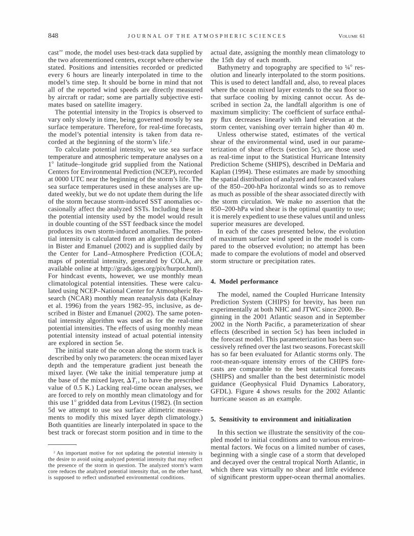
Figure 16 presents a histogram of root-mean-squareintensity errors accumulated over all events, comparingeach storm’s simulated wind speed to the best-track es-timate at the time each storm reached its maximum in-tensity. There is a slight, but statistically insignificantdecrease in rms error when daily values of potentialintensity are used. There is no significant decrease inthe number of very large errors. We did encounter asmall number of events for which the departures of po-tential intensity from monthly mean climatology werelarge and had a correspondingly large effect on simu-lated storm intensity. The most extreme case in our da-taset was that of Hurricane Floyd in 1981 for which thedifference between the simulated intensities using thedaily and monthly mean potential intensities was as


FIG. 16. Histogram showing the number of cases as a function ofthe magnitude of the rms wind speed error, measured at the time ofthe peak wind speed during each event, according to the best-trackdata for all 471 storms. The gray bars show errors using monthlyclimatological potential intensity, while the black bars show errorsusing daily values estimated from NCEP reanalysis data.

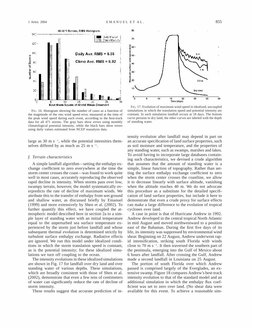
FIG. 17. Evolution of maximum wind speed in idealized, uncoupledsimulations in which the translation speed and potential intensity areconstant. In each simulation landfall occurs at 18 days. The bottomcurve pertains to dry land; the other curves are labeled with the depthof standing water.

large as 30 m s21, while the potential intensities them-selves differed by as much as 25 m s21.

f. Terrain characteristics

A simple landfall algorithm—setting the enthalpy ex-change coefficient to zero everywhere at the time thestorm center crosses the coast—was found to work quitewell in most cases, accurately reproducing the observedrapid decline in intensity. When storms pass over low,swampy terrain, however, the model systematically ov-erpredicts the rate of decline of maximum winds. Weattribute this to the transfer of enthalpy from wet groundand shallow water, as discussed briefly by Emanuel(1999) and more extensively by Shen et al. (2002). Tofurther quantify this effect, we have coupled the at-mospheric model described here in section 2a to a sim-ple layer of standing water with an initial temperatureequal to the unperturbed sea surface temperature ex-perienced by the storm just before landfall and whosesubsequent thermal evolution is determined strictly byturbulent surface enthalpy exchange. Radiative effectsare ignored. We run this model under idealized condi-tions in which the storm translation speed is constant,as is the potential intensity; for these idealized simu-lations we turn off coupling to the ocean.

The intensity evolutions in these idealized simulationsare shown in Fig. 17 for landfall over dry land and overstanding water of various depths. These simulations,which are broadly consistent with those of Shen et al.(2002), demonstrate that even a few tens of centimetersof water can significantly reduce the rate of decline ofstorm intensity.

These results suggest that accurate prediction of in-

tensity evolution after landfall may depend in part onan accurate specification of land surface properties, suchas soil moisture and temperature, and the properties ofany standing water, such as swamps, marshes and lakes.To avoid having to incorporate large databases contain-ing such characteristics, we devised a crude algorithmthat assumes that the amount of standing water is asimple, linear function of topography. Rather than set-ting the surface enthalpy exchange coefficient to zerowhen the storm center crosses the coastline, we allowit to decrease linearly with surface altitude, vanishingwhen the altitude reaches 40 m. We do not advocatethis procedure as a substitute for the detailed specifi-cation of land surface properties, but include it here todemonstrate that even a crude proxy for surface effectscan make a large difference to the evolution of tropicalcyclones over land.

A case in point is that of Hurricane Andrew in 1992.Andrew developed in the central tropical North Atlanticin mid August and moved northwestward to a positioneast of the Bahamas. During the first five days of itslife, its intensity was suppressed by environmental windshear. Beginning on 22 August, Andrew underwent rap-id intensification, striking south Florida with windsclose to 70 m s21. It then traversed the southern part ofthe peninsula, emerging into the Gulf of Mexico about6 hours after landfall. After crossing the Gulf, Andrewmade a second landfall in Louisiana on 25 August.

The portion of south Florida over which Andrewpassed is comprised largely of the Everglades, an ex-tensive swamp. Figure 18 compares Andrew’s best-trackintensity evolution to that of the standard model and anadditional simulation in which the enthalpy flux coef-ficient was set to zero over land. (No shear data wereavailable for this event. To achieve a reasonable sim-


FIG. 18. Evolution of the maximum surface wind speed in Hurri-cane Andrew, 1992. Solid curve shows best-track estimate, dashedcurve shows model simulation in which the enthalpy exchange co-efficient is zero over land, and dashed–dotted curve shows simulationwith the exchange coefficient decreasing linearly with increasing sur-face altitude. Solid black bar at bottom left shows initialization periodin which the model is matched to observations.

FIG. 19. Evolution of the maximum surface wind speed in Hurri-cane Allen, 1980. Solid curve shows best-track estimate, dashed curveshows model simulation. Solid black bar at bottom left shows ini-tialization period in which model is matched to observations.

ulation, the matching interval was extended over muchof the early life of the storm, during which it was strong-ly affected by shear.) The two simulations differ greatlyafter landfall in south Florida. Our crude algorithmclearly improves the intensity hindcast, though it un-derpredicts the rate of decline of Andrew’s intensityafter landfall in Louisiana.

Although our land surface flux algorithm is crude,these results, taken together with the more detailed anal-ysis of Shen et al. (2002), clearly demonstrate the im-portance of accounting for land surface characteristicsin predicting tropical cyclone intensity evolution overland.

g. Internal variability

Although we have proceeded under the premise thatmost observed intensity variations of tropical cyclonesarise from interaction with their environment, it is wellknown that internal features such as concentric eyewallcycles are often associated with large intensity fluctu-ations. It is not always clear whether eyewall cyclesthemselves result strictly from internal instabilities orwhether they are triggered and/or controlled by envi-ronmental interactions. Here we attempt to simulateHurricane Allen of 1980, which had several eyewallreplacement cycles, as documented by Willoughby etal. (1982). The results of this simulation are comparedto observations in Fig. 19. As in the observed storm,the simulation of Allen undergoes several intensity os-cillations that in some ways resemble concentric eyewallcycles. [The ability of this model to produce concentriceyewall-like phenomena was documented by Emanuel(1995a).] While the amplitude of these oscillations is

similar to that of the observed cycles, their phase seemsrandomly related to the observed phase. As might beexpected, the phase of the predicted oscillations provesquite sensitive to environmental and initial conditions,suggesting that the modeled phenomenon is indeed aninternal instability. Detailed examination of the modelfields reveals little in the way of environmental pertur-bations along Allen’s track: the potential intensity wasnearly constant and, although Allen passed close to landmasses (e.g., Jamaica), the model has no way of sim-ulating land interactions unless the storm center passesover land. This further supports the idea that the inten-sity fluctuations in the simulation of Allen are indeedinternally driven.

6. Summary

A simple coupled model has been used to explore thesensitivity of tropical cyclone intensity evolution to ini-tialization and to a variety of environmental factors.Although the atmospheric component of the model isaxisymmetric and therefore cannot directly include en-vironmental wind shear, we developed and tested a pa-rameterization of shear that attempts to account for theventilation of low entropy air through the storm core atmid levels. The coupled model with the shear param-eterization was run experimentally at the National Hur-ricane Center and at the Joint Typhoon Warning Centerand, in the Atlantic region, was found to be about asskillful as statistical forecasts and better than other de-terministic guidance. Experience with the model showsit to perform well when there is little environmentalshear and when storms move over an ocean whose upperthermal structure does not depart much from climatol-ogy. Under these conditions, the model is not overlysensitive to the way in which it is initialized, but in most


circumstances the coupling to the ocean is crucial toobtain good results. When substantial shear is present,on the other hand, the modeled intensity proves sensitiveboth to the magnitude of the shear itself and to initialand environmental conditions and shows a tendency to-ward bimodal intensity distributions. This supports theexperience of hurricane forecasters, who place great em-phasis on the importance of shear. These results suggestthat forecasts are rendered increasingly uncertain in thepresence of shear, unless the shear is so strong as toprevent development in any reasonable environment. Apotentially important source of uncertainty when sub-stantial shear is present is the poorly observed humidityof the middle troposphere.

Accurate forecasts of tropical cyclone intensity re-quire not only good forecasts of environmental windsbut good knowledge of upper-ocean thermal structure.Although we could only show a few cases here, we haveencountered quite a few events in which climatologicalupper-ocean thermal conditions were inadequate for ac-curate intensity prediction. We believe that the impor-tance of tropical cyclone intensity prediction justifiesthe inclusion of upper-ocean temperature and salinitymeasurements in routine airborne reconnaissance mis-sions.

Bathymetry is important where water depths are suf-ficiently small to limit the downward increase of mixedlayer depths by entrainment, as may happen where sea-floors shoal gradually toward coastlines or where stormsapproach the coast obliquely.

With the exception of a very small percentage ofstorms, we have not found much systematic differencebetween forecasts made using real-time potential inten-sity and those made using monthly climatological po-tential intensity. This perhaps reflects the relativelysmall interannual variability of sea surface temperaturesin tropical cyclone-prone regions.

The spindown of storms after landfall appears to beaffected by the presence of standing water, such asswamps and lakes, and is probably similarly affectedby soil moisture content and, perhaps, soil temperature.Detailed forecasts of tropical cyclone evolution overland probably require accurate specification of land sur-face characteristics.

In a few cases, notably that of Hurricane Allen in1980, we found evidence of important internal vari-ability, mostly taking the form of concentric eyewallcycles. Because such cycles have comparatively shorttime scales, they are not predictable responses to en-vironmental fluctuations and, as such, they compromisethe overall predictability of storm intensity. In our lim-ited experience, this mode of variability appears mostlyin intense storms that remain in benign environmentsfor long periods; otherwise, storm intensity is mostlycontrolled by its environment. It should be noted thatnot all eyewall replacement cycles that occur in thismodel develop spontaneously; some occur in response

to strong environmental stimulation, such as passageover an island or peninsula.

The axisymmetry of our atmospheric model precludesthe simulation of baroclinic effects such as trough in-teractions, which are often cited as primary causes ofintensity change (e.g., Molinari and Vollaro, 1989, 1990,1995). The undersimulation of Hurricane Michelle’s latestage intensity (Fig. 10) suggests that such interactionscan indeed be important. Our coupled model may provean ideal tool for isolating such effects, as it attempts toaccount for most of the other processes thought to beimportant; thus baroclinic effects may be a major sourceof systematic error. This will be the subject of futurework by our group.

Finally, we caution against considering the variousenvironmental influences on storm intensity as operatingindependently from each other. For example, shear, insuppressing storm intensity, also suppresses ocean feed-back; the sudden cessation of shearing can then lead tomore rapid intensification and, briefly, to greater inten-sity than could have been reached had shear been absentaltogether. These, and similar effects, are also the sub-ject of continuing investigation by our group.

Acknowledgments. The authors thank Dr. Lars Schadefor providing his coupled model and advice on usingit; Hugh Willoughby for helpful advice and comments;Ed Rappaport, Fiona Horsfal, and Michelle Mainelli fortheir help in running CHIPS at the National HurricaneCenter; Buck Sampson of the Monterey Naval ResearchLaboratory; and Don Schiber, Donald Laframboise,Chris Cantrell, and Steve Vilpors of the Naval PacificMeteorology and Oceanography Center for assistancein running CHIPS at the Joint Typhoon Warning Center.We are also grateful for helpful comments from twoanonymous reviewers.

REFERENCES

Alamaro, M., K. Emanuel, J. Colton, W. McGillis, and J. B. Edson,2002: Experimental investigation of air–sea transfer of momen-tum and enthalpy at high wind speed. Preprints, 25th Conf. onHurricanes and Tropical Meteorology, San Diego, CA, Amer.Meteor. Soc., 667–668.

Bender, M. A., and I. Ginis, 2000: Real-case simulations of hurricane–ocean interaction using a high-resolution coupled model: Effectson hurricane intensity. Mon. Wea. Rev., 128, 917–946.

Bister, M., and K. A. Emanuel, 1998: Dissipative heating and hur-ricane intensity. Meteor. Atmos. Phys., 50, 233–240.

——, and ——, 2002: Low frequency variability of tropical cyclonepotential intensity 2. Climatology for 1982–1995. J. Geophys.Res., 107, 4621, doi:10.1029/2001JD000780.

Cooper, C., and J. D. Thompson, 1989: Hurricane-generated currentson the outer continental shelf. Part I: Model formulation andverification. J. Geophys. Res., 94, 12 513–12 539.

DeMaria, M., and J. Kaplan, 1994: A statistical hurricane intensityprediction scheme (SHIPS) for the Atlantic basin. Wea. Fore-casting, 9, 209–220.

——, and ——, 1997: An operational evaluation of a statistical hur-ricane intensity prediction scheme (SHIPS). Preprints, 22d Conf.on Hurricanes and Tropical Meteorology, Fort Collins, CO,Amer. Meteor. Soc., 280–281.


Emanuel, K. A., 1986: An air–sea interaction theory for tropicalcyclones. Part I: Steady-state maintenance. J. Atmos. Sci., 3,585–605.

——, 1988: The maximum intensity of hurricanes. J. Atmos. Sci.,45, 1143–1155.

——, 1995a: The behavior of a simple hurricane model using a con-vective scheme based on subcloud-layer entropy equilibrium. J.Atmos. Sci., 52, 3959–3968.

——, 1995b: Sensitivity of tropical cyclones to surface exchangecoefficients and a revised steady-state model incorporating eyedynamics. J. Atmos. Sci., 52, 3969–3976.

——, 1999: Thermodynamic control of hurricane intensity. Nature,401, 665–669.

Frank, W. M., and E. A. Ritchie, 2001: Effects of vertical wind shearon the intensity and structure of numerically simulated hurri-canes. Mon. Wea. Rev., 129, 2249–2269.

Gallacher, P. C., R. Rotunno, and K. A. Emanuel, 1989: Tropicalcyclogenesis in a coupled ocean–atmosphere model. Preprints,18th Conf. on Hurricanes and Tropical Meteorology, San Diego,CA, Amer. Meteor. Soc., 121–122.

Jones, S. C., 2000: The evolution of vortices in vertical shear. PartIII: Baroclinic vortices. Quart. J. Roy. Meteor. Soc., 126, 3161–3185.

Kalnay, E., and Coauthors, 1996: The NCEP/NCAR 40-Year Re-analysis Project. Bull. Amer. Meteor. Soc., 77, 437–471.

Khain, A., and I. Ginis, 1991: The mutual response of a movingtropical cyclone and the ocean. Beitr. Phys. Atmos., 64, 125–141.

Large, W. G., and S. Pond, 1982: Sensible and latent heat flux mea-surements over the ocean. J. Phys. Oceanogr., 12, 464–482.

Leipper, D. F., 1967: Observed ocean conditions and Hurricane Hilda,1964. J. Atmos. Sci., 24, 182–196.

Levitus, S., 1982: Climatological Atlas of the World Ocean. NOAAProf. Paper 13, 173 pp. and 17 microfiche.

Molinari, J., and D. Vollaro, 1989: External influences on hurricaneintensity. Part I: Outflow layer eddy angular momentum fluxes.J. Atmos. Sci., 46, 1093–1105.

——, and ——, 1990: External influences on hurricane intensity. Part

II: Vertical structure and response of the hurricane vortex. J.Atmos. Sci., 47, 1902–1918.

——, and ——, 1995: External influences on hurricane intensity. PartIII: Potential vorticity structure. J. Atmos. Sci., 52, 3593–3606.

Nong, S., and K. Emanuel, 2003: Concentric eyewalls in hurricanes.Quart. J. Roy. Meteor. Soc., 129, 3328–3338.

Price, J. F., 1981: Upper ocean response to a hurricane. J. Phys.Oceanogr., 11, 153–175.

Raymond, D. J., 1995: Regulation of moist convection over the westPacific warm pool. J. Atmos. Sci., 52, 3945–3959.

Schade, L. R., 1994: The ocean’s effect on hurricane intensity. Ph.D.thesis, Massachusetts Institute of Technology, 127 pp.

——, 1997: A physical interpretation of SST-feedback. Preprints, 22dConf. on Hurricanes and Tropical Meteorology, Fort Collins,CO, Amer. Meteor. Soc., 439–440.

——, and K. A. Emanuel, 1999: The ocean’s effect on the intensityof tropical cyclones: Results from a simple coupled atmosphere–ocean model. J. Atmos. Sci., 56, 642–651.

Schubert, W. H., and J. J. Hack, 1983: Transformed Eliassen-balancedvortex model. J. Atmos. Sci., 40, 1571–1583.

Shay, L. K., G. J. Goni, and P. G. Black, 2000: Effects of a warmoceanic feature on Hurricane Opal. Mon. Wea. Rev., 128, 1366–1383.

Shen, W., I. Ginis, and R. E. Tuleya, 2002: A numerical investigationof land surface water on landfalling hurricanes. J. Atmos. Sci.,59, 789–802.

Shutts, G. J., 1981: Hurricane structure and the zero potential vorticityapproximation. Mon. Wea. Rev., 109, 324–329.

Simpson, R. H., and H. Riehl, 1958: Mid-tropospheric ventilation asa constraint on hurricane development and maintenance. Proc.Tech. Conf. on Hurricanes, Miami Beach, FL, Amer. Meteor.Soc., D4-1–D4-10.

Willoughby, H. E., and P. G. Black, 1996: Hurricane Andrew inFlorida: Dynamics of a disaster. Bull. Amer. Meteor. Soc., 77,643–652.

——, J. A. Clos, and M. G. Shoreibah, 1982: Concentric eyes, sec-ondary wind maxima, and the evolution of the hurricane vortex.J. Atmos. Sci., 39, 395–411.

Environmental Control of Tropical Cyclone Intensity

Documents

Transcript of Environmental Control of Tropical Cyclone Intensity