The Affine Arbitrage-Free Class ofNelson-Siegel Term Structure Models

Jens H. E. ChristensenFrancis X. Diebold

Glenn D. Rudebusch

Term Structure Modeling and the Lower Bound Problem

Day 1: Term Structure Modeling in Normal Times

Lecture I.2

European University InstituteFlorence, September 7, 2015

The views expressed here are solely the responsibility of the authors and should not be interpreted as reflecting the views

of the Federal Reserve Bank of San Francisco or the Board of Governors of the Federal Reserve System. 1 / 37

Motivation

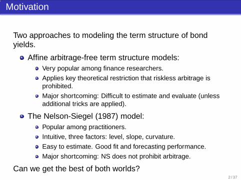
Two approaches to modeling the term structure of bondyields.

Affine arbitrage-free term structure models:Very popular among finance researchers.

Applies key theoretical restriction that riskless arbitrage isprohibited.

Major shortcoming: Difficult to estimate and evaluate (unlessadditional tricks are applied).

The Nelson-Siegel (1987) model:Popular among practitioners.

Intuitive, three factors: level, slope, curvature.

Easy to estimate. Good fit and forecasting performance.

Major shortcoming: NS does not prohibit arbitrage.

Can we get the best of both worlds?2 / 37

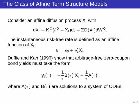
The Class of Affine Term Structure Models

Consider an affine diffusion process Xt with

dXt = K Q(θQ − Xt)dt + ΣD(Xt )dW Qt .

The instantaneous risk-free rate is defined as an affinefunction of Xt :

rt = ρ0 + ρ′1Xt .

Duffie and Kan (1996) show that arbitrage-free zero-couponbond yields must take the form

yt(τ) = −1τ

B(τ)′Xt −1τ

A(τ),

where A(τ) and B(τ) are solutions to a system of ODEs.

3 / 37

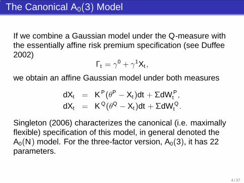
The Canonical A0(3) Model

If we combine a Gaussian model under the Q-measure withthe essentially affine risk premium specification (see Duffee2002)

Γt = γ0 + γ1Xt ,

we obtain an affine Gaussian model under both measures

dXt = K P(θP − Xt)dt + ΣdW Pt ,

dXt = K Q(θQ − Xt)dt + ΣdW Qt .

Singleton (2006) characterizes the canonical (i.e. maximallyflexible) specification of this model, in general denoted theA0(N) model. For the three-factor version, A0(3), it has 22parameters.

4 / 37

Problem with the Canonical A0(3) Model

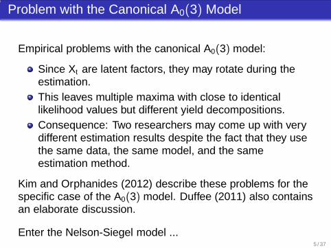
Empirical problems with the canonical A0(3) model:

Since Xt are latent factors, they may rotate during theestimation.This leaves multiple maxima with close to identicallikelihood values but different yield decompositions.Consequence: Two researchers may come up with verydifferent estimation results despite the fact that they usethe same data, the same model, and the sameestimation method.

Kim and Orphanides (2012) describe these problems for thespecific case of the A0(3) model. Duffee (2011) also containsan elaborate discussion.

Enter the Nelson-Siegel model ...5 / 37

The Nelson-Siegel Term Structure Model (1)

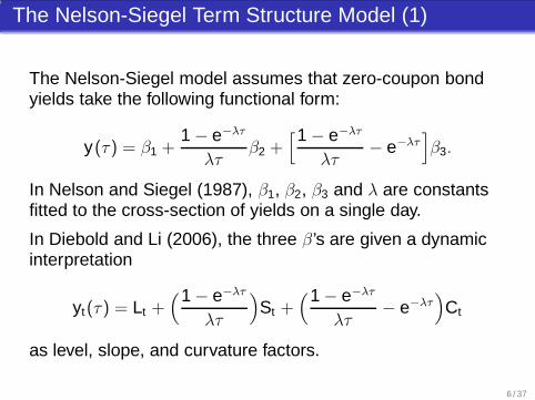
The Nelson-Siegel model assumes that zero-coupon bondyields take the following functional form:

y(τ) = β1 +1 − e−λτ

λτβ2 +

[1 − e−λτ

λτ− e−λτ

]

β3.

In Nelson and Siegel (1987), β1, β2, β3 and λ are constantsfitted to the cross-section of yields on a single day.

In Diebold and Li (2006), the three β’s are given a dynamicinterpretation

yt(τ) = Lt +(1 − e−λτ

λτ

)

St +(1 − e−λτ

λτ− e−λτ

)

Ct

as level, slope, and curvature factors.

6 / 37

The Nelson-Siegel Term Structure Model (2)

0 2 4 6 8 10

0.0

0.2

0.4

0.6

0.8

1.0

Time to maturity in years

Fac

tor

load

ing

Lambda = 1

Lambda = 0.5

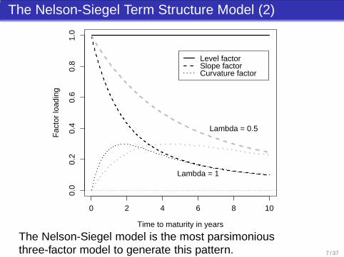
Level factor Slope factor Curvature factor

The Nelson-Siegel model is the most parsimoniousthree-factor model to generate this pattern. 7 / 37

The Nelson-Siegel Term Structure Model (3)

Pros: Parsimonious, yet very flexible. Good fit. Intuitiveinterpretation of parameter and state variables.

Cons: Trouble fitting long maturities. More importantly,Filipovic (1999) proves that it cannot be made arbitrage-freefor any dynamics.

Can we overcome the cons (while maintaining the pros)?

8 / 37

The Affine Arbitrage-Free Class of NS Models (1)

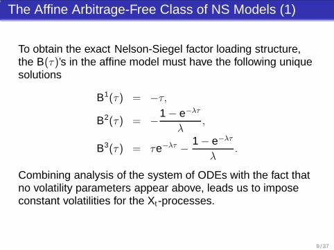
To obtain the exact Nelson-Siegel factor loading structure,the B(τ)’s in the affine model must have the following uniquesolutions

B1(τ) = −τ,

B2(τ) = −1 − e−λτ

λ,

B3(τ) = τe−λτ −1 − e−λτ

λ.

Combining analysis of the system of ODEs with the fact thatno volatility parameters appear above, leads us to imposeconstant volatilities for the Xt -processes.

9 / 37

The Affine Arbitrage-Free Class of NS Models (2)

Given a constant volatility specification, the ODEs for B(τ)reduce to:

dB(τ)

dτ= −ρ1 − (K Q)′B(τ), B(0) = 0.

Now, manipulate ρ1 and K Q until the desired result isobtained.

Note: Diebold, Piazzesi and Rudebusch (2005) describe asolution for the two-factor case.

10 / 37

The Affine Arbitrage-Free Class of NS Models (3)

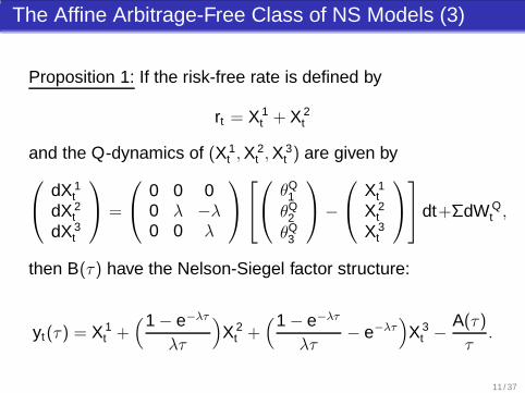
Proposition 1: If the risk-free rate is defined by

rt = X 1t + X 2

t

and the Q-dynamics of (X 1t ,X

2t ,X

3t ) are given by

dX 1t

dX 2t

dX 3t

=

0 0 00 λ −λ

0 0 λ

θQ1θQ

2θQ

3

−

X 1t

X 2t

X 3t

dt+ΣdW Qt ,

then B(τ) have the Nelson-Siegel factor structure:

yt(τ) = X 1t +

(1 − e−λτ

λτ

)

X 2t +

(1 − e−λτ

λτ− e−λτ

)

X 3t −

A(τ)τ

.

11 / 37

The Affine Arbitrage-Free Class of NS Models (4)

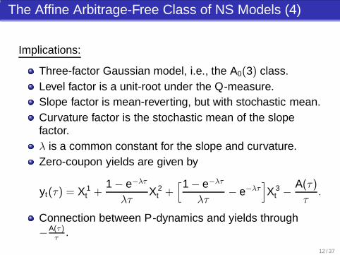
Implications:

Three-factor Gaussian model, i.e., the A0(3) class.Level factor is a unit-root under the Q-measure.Slope factor is mean-reverting, but with stochastic mean.Curvature factor is the stochastic mean of the slopefactor.λ is a common constant for the slope and curvature.Zero-coupon yields are given by

yt(τ) = X 1t +

1 − e−λτ

λτX 2

t +[1 − e−λτ

λτ− e−λτ

]

X 3t −

A(τ)τ

.

Connection between P-dynamics and yields through−A(τ)

τ.

12 / 37

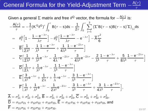
General Formula for the Yield-Adjustment Term −A(τ)τ

Given a general Σ matrix and free θQ vector, the formula for −A(τ )τ

is:

−

A(τ )τ

= −

1τ(K Q

θQ)′

∫ τ

0B(τ − s)ds −

12τ

∫ τ

0

3∑

j=1

(

Σ′B(τ − s)B(τ − s)′Σ)

j,jds

= θQ2

[

1 −

1 − e−λτ

λτ

]

− θQ3

[1 − e−λτ

λτ− e−λτ

]

− Aτ 2

6

− B[ 1

2λ2−

1λ3

1 − e−λτ

τ+

14λ3

1 − e−2λτ

τ

]

− C[ 1

2λ2+

1λ2

e−λτ−

14λ

τe−2λτ−

34λ2

e−2λτ−

2λ3

1 − e−λτ

τ+

58λ3

1 − e−2λτ

τ

]

− D[ 1

2λτ +

1λ2

e−λτ−

1λ3

1 − e−λτ

τ

]

− E[ 3λ2

e−λτ +1

2λτ +

1λτe−λτ

−

3λ3

1 − e−λτ

τ

]

− F[ 1λ2

+1λ2

e−λτ−

12λ2

e−2λτ−

3λ3

1 − e−λτ

τ+

34λ3

1 − e−2λτ

τ

]

,

A = σ211 + σ2

12 + σ213, B = σ2

21 + σ222 + σ2

23, C = σ231 + σ2

32 + σ233,

D = σ11σ21 + σ12σ22 + σ13σ23, E = σ11σ31 + σ12σ32 + σ13σ33, and

F = σ21σ31 + σ22σ32 + σ23σ33. 13 / 37

Identification of Parameters in the AFNS Model Class

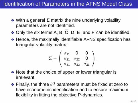
With a general Σ matrix the nine underlying volatilityparameters are not identified.

Only the six terms A, B, C, D, E , and F can be identified.

Hence, the maximally identifiable AFNS specification hastriangular volatility matrix:

Σ =

σ11 0 0σ21 σ22 0σ31 σ32 σ33

.

Note that the choice of upper or lower triangular isirrelevant.

Finally, the three θQ parameters must be fixed at zero tohave econometric identification and to ensure maximumflexibility in fitting the objective P-dynamics.

14 / 37

Link between the Canonical A0(3) and AFNS Models

The maximally flexible arbitrage-free NS model has 19parameters:

18 describe the P-dynamics;λ determines the Q-dynamics.

This is close to the 22 maximally identifiable.

Despite this fact, we do not encounter the type of estimationproblems reported for the maximally flexible A0(3) model.

Possible explanations seem to involve:The factors are clearly identified as level, slope andcurvature by the Nelson-Siegel yield function.Without rotation of the state variables, the parameters forthe P-dynamics remain stable during estimation.Consequence: no multiple maxima - stable parameterestimates across subsamples.

15 / 37

Data

We use end-of-month unsmoothed Fama-Bliss zero-couponyields covering the period from January 1987 to December2002 with a total of 16 different constant maturities (in years)

{0.25, 0.5, 0.75, 1, 1.5, 2, 3, 4, 5, 7, 8, 9, 10, 15, 20, 30}.

The long end is well represented because that is where weexpect ’in-sample’ performance differences to appearbetween the standard NS models and the arbitrage-freeequivalents.

16 / 37

Horse Race: Model Specifications (1)

We estimate two standard dynamic Nelson-Siegel (DNS)models that are not arbitrage-free:

1 DNS indep. factors: The three factors are independentAR(1) processes, see Diebold and Li (2006).

2 DNS corr. factors: The three factors follow a VAR(1)specification with correlated shocks, see Diebold,Rudebusch and Aruoba (2006).

For the arbitrage-free Nelson-Siegel (AFNS) model weestimate the two corresponding specifications.

17 / 37

Horse Race: Model Specifications (2)

The two arbitrage-free models are:

1 AFNS with independent factors.2 AFNS with correlated factors (full K P-matrix and

triangular Σ).

The last specification is the maximally flexible specification ofthe AFNS model class.

We identify the AFNS models by fixing θQ = 0 while letting θP

be determined by the estimation.

We show that this identification is without loss of generality.

18 / 37

Estimation Method

All the models considered have affine state andmeasurement equations and Gaussian measurement andstate equation errors.

Therefore, the Kalman filter is an efficient and consistentestimator.

Stationarity of the state variables is imposed in theestimation. Thus, the Kalman filter is started at theunconditional mean and covariance matrix.

19 / 37

RMSE of Fitted Yields (bps)

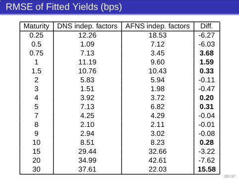
Maturity DNS indep. factors AFNS indep. factors Diff.0.25 12.26 18.53 -6.270.5 1.09 7.12 -6.030.75 7.13 3.45 3.68

1 11.19 9.60 1.591.5 10.76 10.43 0.332 5.83 5.94 -0.113 1.51 1.98 -0.474 3.92 3.72 0.205 7.13 6.82 0.317 4.25 4.29 -0.048 2.10 2.11 -0.019 2.94 3.02 -0.0810 8.51 8.23 0.2815 29.44 32.66 -3.2220 34.99 42.61 -7.6230 37.61 22.03 15.58

20 / 37

RMSE of Fitted Yields (bps)

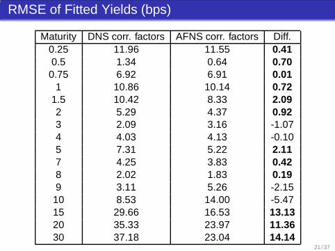
Maturity DNS corr. factors AFNS corr. factors Diff.0.25 11.96 11.55 0.410.5 1.34 0.64 0.700.75 6.92 6.91 0.01

1 10.86 10.14 0.721.5 10.42 8.33 2.092 5.29 4.37 0.923 2.09 3.16 -1.074 4.03 4.13 -0.105 7.31 5.22 2.117 4.25 3.83 0.428 2.02 1.83 0.199 3.11 5.26 -2.1510 8.53 14.00 -5.4715 29.66 16.53 13.1320 35.33 23.97 11.3630 37.18 23.04 14.14

21 / 37

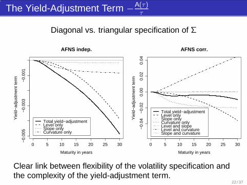
The Yield-Adjustment Term −A(τ)τ

Diagonal vs. triangular specification of Σ

0 5 10 15 20 25 30

−0.

005

−0.

003

−0.

001

AFNS indep.

Maturity in years

Yie

ld−

adju

stm

ent t

erm

Total yield−adjustment Level only Slope only Curvature only

0 5 10 15 20 25 30−

0.04

−0.

020.

000.

020.

04

AFNS corr.

Maturity in years

Yie

ld−

adju

stm

ent t

erm

Total yield−adjustment Level only Slope only Curvature only Level and slope Level and curvature Slope and curvature

Clear link between flexibility of the volatility specification andthe complexity of the yield-adjustment term.

22 / 37

Summary of In-Sample Fit

DNS indep. vs. AFNS indep.:The AFNS model is restricted through the connectionbetween Σ and the yield function, and it gets very little helpfrom the yield adjustment term.

DNS corr. vs. AFNS corr.:With a flexible volatility structure the yield adjustment termimproves fit of long-term yields. To some extent, this frees upthe level factor which leads to improved fit for shorter termyields.

Does the improvement for the correlated-factor AFNS modelhold up when we move out of sample?

23 / 37

Out-of-Sample Forecasts (1)

Starting December 1996 we re-estimate all four modelsadding a month of extra observations every time, a total of 73estimations for each model.

For every estimation and every model we forecast the yieldsof the following maturities (in years)

{0.25, 1, 3, 5, 10, 30}

at the 1-month, the 6-month, and the 12-month horizons.

Thus, for each of the three forecast horizons, we get a totalnumber of forecast errors of 72, 67, and 61, respectively.

We use RMSE of the forecast errors as forecast performancemeasure.

24 / 37

Out-of-Sample Forecasts (2)

DNS indep. vs. AFNS indep.

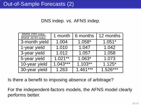
RMSE DNS indep.RMSE AFNS indep. 1 month 6 months 12 months3-month yield 1.004 1.058* 1.051*1-year yield 1.010 1.047 1.0423-year yield 1.012 1.057 1.0585-year yield 1.021** 1.063* 1.07310-year yield 1.043*** 1.103** 1.125*30-year yield 1.263 1.461*** 1.526***

Is there a benefit to imposing absence of arbitrage?

For the independent-factors models, the AFNS model clearlyperforms better.

25 / 37

Out-of-Sample Forecasts (3)

DNS corr. vs. AFNS corr.

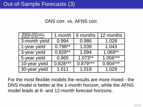
RMSE DNS corr.RMSE AFNS corr. 1 month 6 months 12 months3-month yield 0.994 0.986 1.0281-year yield 0.798** 1.039 1.0433-year yield 0.828** 1.094 1.069**5-year yield 0.965 1.073** 1.056***10-year yield 0.828*** 0.879*** 0.904***30-year yield 1.011 1.019 1.029

For the most flexible models the results are more mixed - theDNS model is better at the 1-month horizon, while the AFNSmodel leads at 6- and 12-month forecast horizons.

26 / 37

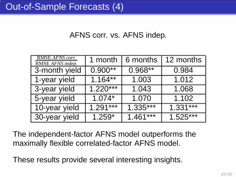
Out-of-Sample Forecasts (4)

AFNS corr. vs. AFNS indep.

RMSE AFNS corr.RMSE AFNS indep. 1 month 6 months 12 months3-month yield 0.900** 0.968** 0.9841-year yield 1.164** 1.003 1.0123-year yield 1.220*** 1.043 1.0685-year yield 1.074* 1.070 1.10210-year yield 1.291*** 1.335*** 1.331***30-year yield 1.259* 1.461*** 1.525***

The independent-factor AFNS model outperforms themaximally flexible correlated-factor AFNS model.

These results provide several interesting insights.

27 / 37

Out-of-Sample Forecast Summary (1)

Despite its in-sample superiority, the maximally flexibleAFNS model is poor at forecasting out of sample.

This is a point that has general validity for othermaximally flexible affine three-factor models.

This type of model produces a yield adjustment term thatdelivers clearly superior in-sample performance,particularly for long maturities.

Ironically, it is this same yield adjustment term thatresults in this model’s poor out of sample performancefor two reasons:

1 The required adjustment term change out of sample.

2 The level factor, in particular, is less persistent.

28 / 37

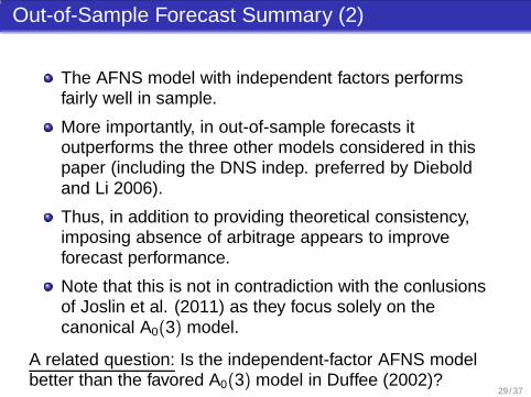
Out-of-Sample Forecast Summary (2)

The AFNS model with independent factors performsfairly well in sample.

More importantly, in out-of-sample forecasts itoutperforms the three other models considered in thispaper (including the DNS indep. preferred by Dieboldand Li 2006).

Thus, in addition to providing theoretical consistency,imposing absence of arbitrage appears to improveforecast performance.

Note that this is not in contradiction with the conlusionsof Joslin et al. (2011) as they focus solely on thecanonical A0(3) model.

A related question: Is the independent-factor AFNS modelbetter than the favored A0(3) model in Duffee (2002)?

29 / 37

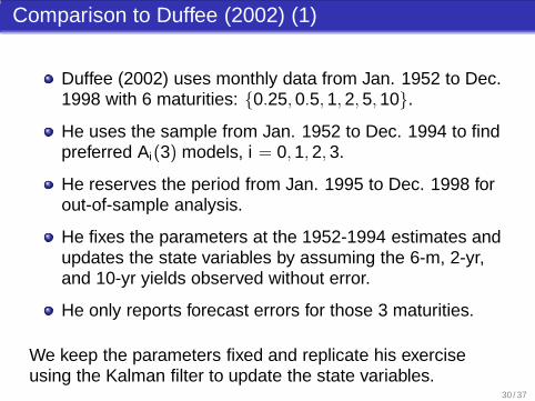
Comparison to Duffee (2002) (1)

Duffee (2002) uses monthly data from Jan. 1952 to Dec.1998 with 6 maturities: {0.25, 0.5, 1, 2, 5, 10}.

He uses the sample from Jan. 1952 to Dec. 1994 to findpreferred Ai(3) models, i = 0, 1, 2, 3.

He reserves the period from Jan. 1995 to Dec. 1998 forout-of-sample analysis.

He fixes the parameters at the 1952-1994 estimates andupdates the state variables by assuming the 6-m, 2-yr,and 10-yr yields observed without error.

He only reports forecast errors for those 3 maturities.

We keep the parameters fixed and replicate his exerciseusing the Kalman filter to update the state variables.

30 / 37

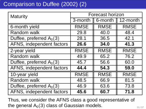
Comparison to Duffee (2002) (2)

Forecast horizonMaturity3-month 6-month 12-month

6-month yield RMSE RMSE RMSERandom walk 29.8 40.0 48.4Duffee, preferred A0(3) 28.1 36.5 42.1AFNS, independent factors 26.6 34.0 41.32-year yield RMSE RMSE RMSERandom walk 49.9 65.2 76.2Duffee, preferred A0(3) 45.7 56.6 60.0AFNS, independent factors 44.4 54.3 59.010-year yield RMSE RMSE RMSERandom walk 48.5 66.9 81.5Duffee, preferred A0(3) 46.9 63.6 73.8AFNS, independent factors 45.6 60.7 71.8

Thus, we consider the AFNS class a good representative ofthe general A0(3) class of Gaussian models. 31 / 37

Conclusion

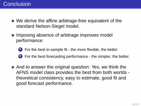
We derive the affine arbitrage-free equivalent of thestandard Nelson-Siegel model.

Imposing absence of arbitrage improves modelperformance:

1 For the best in-sample fit - the more flexible, the better.

2 For the best forecasting performance - the simpler, the better.

And to answer the original question: Yes, we think theAFNS model class provides the best from both worlds -theoretical consistency, easy to estimate, good fit andgood forecast performance.

32 / 37

Why Nelson-Siegel?

0 2 4 6 8 10

−0.

4−

0.2

0.0

0.2

0.4

Time to maturity in years

Load

ing

0 2 4 6 8 10

−0.

4−

0.2

0.0

0.2

0.4

Time to maturity in years

Load

ing

First P.C. Second P.C. Thrid P.C.

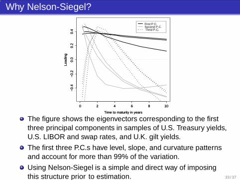
The figure shows the eigenvectors corresponding to the firstthree principal components in samples of U.S. Treasury yields,U.S. LIBOR and swap rates, and U.K. gilt yields.

The first three P.C.s have level, slope, and curvature patternsand account for more than 99% of the variation.

Using Nelson-Siegel is a simple and direct way of imposingthis structure prior to estimation. 33 / 37

Are the Parameter Restrictions in AFNS Models Valid?

1997 1998 1999 2000 2001 2002 2003

010

020

030

040

050

0

End of sample

LR te

st

99.9 percentile in chi^2 distribution, df = 9

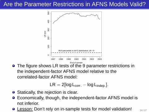
The figure shows LR tests of the 9 parameter restrictions inthe independent-factor AFNS model relative to thecorrelated-factor AFNS model:

LR = 2[log Lcorr . − log Lindep.].

Statically, the rejection is clear.Economically, though, the independent-factor AFNS model isnot inferior.Lesson: Don’t rely on in-sample tests for model validation! 34 / 37

Robustness to Data (1)

1988 1990 1992 1994 1996 1998

0.04

0.06

0.08

0.10

0.12

Est

imat

ed fa

ctor

val

ue

Daily GSW 1985−2011, CLR (2014) Weekly H.15 & GSW 1985−2014, CR (2015) Unsmoothed Fama−Bliss 1987−2002, CDR (2011) McCulloch−Kwon 1952−1998, Duffee (2002)

1988 1990 1992 1994 1996 1998

−0.

06−

0.04

−0.

020.

000.

02

Est

imat

ed fa

ctor

val

ue

Daily GSW 1985−2011, CLR (2014) Weekly H.15 & GSW 1985−2014, CR (2015) Unsmoothed Fama−Bliss 1987−2002, CDR (2011) McCulloch−Kwon 1952−1998, Duffee (2002)

Daily GSW data, Jan. 2, 1985 to Jun. 30, 2011,{0.25,0.5,1,2,3,5,7,10}, CLR (2014).Weekly H.15 & GSW data, Jan. 4, 1985 to Oct. 31, 2014,{0.25,0.5,1,2,3,5,7,10}, CR (2015).Monthly unsmoothed Fama-Bliss data, Jan. 1987 to Dec.2002, 16 maturities, CDR (2011).Monthly McCulloch-Kwan data, Jan. 1952 to Dec. 1998, 6maturities, Duffee (2002). 35 / 37

Robustness to Data (2)

1988 1990 1992 1994 1996 1998

−0.

06−

0.04

−0.

020.

000.

020.

040.

06

Est

imat

ed v

alue

of C

(t)

Daily GSW 1985−2011, CLR (2014) Weekly H.15 & GSW 1985−2014, CR (2015) Unsmoothed Fama−Bliss 1987−2002, CDR (2011) McCulloch−Kwon 1952−1998, Duffee (2002)

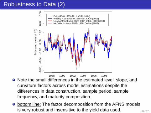
Note the small differences in the estimated level, slope, andcurvature factors across model estimations despite thedifferences in data construction, sample period, samplefrequency, and maturity composition.

bottom line: The factor decomposition from the AFNS modelsis very robust and insensitive to the yield data used. 36 / 37

Advantages of Nelson-Siegel Models

Krippner (2015) shows that AFNS models provide a closeapproximation to any N-dimensional Gaussian model.

Multiple extensions:Cross section: Svensson (1995) and Christensen,Diebold and Rudebusch (2009).

Types of data:

1 Christensen, Lopez and Rudebusch (2010) extend AFNS to fitU.S. Treasuries and TIPS.

2 Christensen, Lopez and Rudebusch (2014b) extend AFNS to fitU.S. Treasuries, corporate bonds, and LIBOR.

Stochastic volatility: Christensen, Lopez and Rudebusch(2014a).

Shadow rates: Christensen and Rudebusch (2015a).

And more to come in the future ... 37 / 37