How Arbitrage-Free is the Nelson-Siegel Model?

Laura Coroneo∗, Ken Nyholm†and Rositsa Vidova-Koleva‡

First version: August 2007This version: June 2008 §

AbstractWe test whether the Nelson and Siegel (1987) yield curve model isarbitrage-free in a statistical sense. Theoretically, the Nelson-Siegelmodel does not ensure the absence of arbitrage opportunities, as shownby Bjork and Christensen (1999). Still, central banks and publicwealth managers rely heavily on it. Using a non-parametric resam-pling technique and zero-coupon yield curve data from the US market,we find that the no-arbitrage parameters are not statistically differentfrom those obtained from the NS model, at a 95 percent confidencelevel. We therefore conclude that the Nelson and Siegel yield curvemodel is compatible with arbitrage-freeness on the US market. To cor-roborate this result, we show that the Nelson-Siegel model performsas well as its no-arbitrage counterpart in an out-of-sample forecastingexperiment.

JEL classification codes: C14, C15, G12Keywords Nelson-Siegel model; No-arbitrage restrictions; affine term struc-ture models; non-parametric test

∗ECARES, Universite Libre de Bruxelles, avenue Roosevelt 50 CP114, B-1050 Brux-elles, Belgium and Department of Economics, University of Bologna, Piazza Scaravilli 1,40126 Bologna, Italy, telephone: +32 2650 3375.

†Risk Management Division, European Central Bank, Kaiserstrasse 29, Frankfurt amMain, Germany, telephone: +49 69 1344 7926.

‡IDEA, Departament d’Economia i d’Historia Economica, Universitat Autonoma deBarcelona, 08193, Bellaterra (Barcelona), Spain, telephone: +49 69 1344 5743.Copyright 2007, Laura Coroneo, Ken Nyholm and Rositsa Vidova-Koleva.The majority of the work on this paper was completed while Laura Coroneo and RositsaVidova-Koleva were visiting the Risk Management Division of the European Central Bank.

§We would like to thank Valentina Corradi, Russel Davidson, David Veredas, andCarsten Tanggaard for helpful comments and suggestions. We also wish to thank par-ticipants at the 2008 Royal Economic Society Conference, the doctoral seminar of theUniversity of Bologna, the internal seminar at ECARES, the 2008 Eastern Finance Asso-ciation Meeting, and the seminar series at CREATES for providing their input. Needlessto say, any remaining errors are our own.

How Arbitrage-Free is the Nelson-Siegel Model?

Abstract

We test whether the Nelson and Siegel (1987) yield curve model is arbitrage-free in a statistical sense. Theoretically, the Nelson-Siegel model does notensure the absence of arbitrage opportunities, as shown by Bjork and Chris-tensen (1999). Still, central banks and public wealth managers rely heavilyon it. Using a non-parametric resampling technique and zero-coupon yieldcurve data from the US market, we find that the no-arbitrage parameters arenot statistically different from those obtained from the NS model, at a 95percent confidence level. We therefore conclude that the Nelson and Siegelyield curve model is compatible with arbitrage-freeness on the US market.To corroborate this result, we show that the Nelson-Siegel model performsas well as its no-arbitrage counterpart in an out-of-sample forecasting exper-iment.

JEL classification codes: C14, C15, G12Keywords Nelson-Siegel model; No-arbitrage restrictions; affine term struc-ture models; non-parametric test

Fixed-income wealth managers in public organizations, investment banks and

central banks rely heavily on Nelson and Siegel (1987) type of models to fit

and forecast yield curves. According to BIS (2005), the central banks of

Belgium, Finland, France, Germany, Italy, Norway, Spain, and Switzerland,

use these models to estimate zero-coupon yield curves. The European Central

Bank (ECB) publishes daily Eurosystem-wide yield curves on the basis of the

Soderlind and Svensson (1997) model, which is an extension of the Nelson-

Siegel model.1 In its foreign reserve management framework the ECB uses a

regime-switching extension of the Nelson-Siegel model, see Bernadell, Coche

and Nyholm (2005).

There are at least four reasons for the popularity of the Nelson-Siegel

model. First, it is easy to estimate. In fact, if the so-called time-decay-

parameter is fixed, then Nelson-Siegel curves are obtained by linear regres-

sion techniques. If this parameter is not fixed, one has to resort to non-linear

regression techniques. In addition, the Nelson-Siegel model by virtue of its

empirical nature, can easily be extended. Second, the model provides by

construction yields for all maturities, i.e. also maturities that are not cov-

ered by the data sample. As such, it lends itself as an interpolation and

extrapolation tool for the analyst who often is interested in yields at matu-

rities that are not directly observable.2 Third, estimated yield curve factors

obtained from the Nelson and Siegel model have intuitive interpretations, as

1For Eurosystem-wide yield curves see http://www.ecb.int/stats/money/yc/html/index.en.html.

2This is relevant e.g. in a situation where fixed-income returns are calculated to takeinto account the roll-down/maturity shortening effect.

2

the level, the slope, and the curvature of the yield curve. This interpretation

is akin to that obtained by a principal component analysis, see e.g. Litter-

man and Scheinkman (1991) and Diebold and Li (2006). Due to its intuitive

appeal estimates and conclusions drawn on the basis of the model are easy

to communicate. Fourth, empirically the Nelson-Siegel model fits data well

and performs well in out-of-sample forecasting exercises, as shown by e.g.

Diebold and Li (2006) and De Pooter, Ravazzolo and van Dijk (2007).

However, despite its empirical merits and wide-spread use in the finance

community, two theoretical concerns can be raised against the Nelson-Siegel

model. First, by conventional standards, it is not arbitrage-free, as shown by

Bjork and Christensen (1999). Second, as demonstrated by Diebold, Ji and

Li (2006b), it falls outside the class of affine yield curve models defined by

Duffie and Kan (1996) and Dai and Singleton (2000).

In its original form, the Nelson and Siegel (1987) model does not pre-

specify any dynamic evolution for the underlying yield curve factors. Rather,

it presents a parsimonious and intuitive description of the forward and spot

yield curve at a given point in time. A dynamic version of the Nelson-

Siegel model is proposed by Diebold and Li (2006), where a time-series model

is suggested to account for the evolution of the level, slope and curvature

factors over time. Data, as opposed to theory, guides the parametrisation of

the introduced time series model. In this case the Nelson-Siegel yield-curve

model can be set in state-space form and estimation can be carried out using

the Kalman filter.

The modelling advance made in Diebold and Li (2006), allows us to better

analyse the connection between the Nelson-Siegel and the classic multi-factor

3

no-arbitrage yield curve models. When viewed through the lens of a state-

space model, this difference becomes clear. Setting the Nelson-Siegel model

in state space form amounts to defining the observation equation, which

translates the yield curve factors into observed yields, as the original Nelson-

Siegel model; the state equation is then represented by a time-series model

for the yield curve factors, e.g. the Vector Autoregressive model of order 1,

VAR(1), as suggested by Diebold and Li (2006). It is important to note that

there is no relationship between the parameters in the observation equation

(also called factor loadings) and the parameters of the state equation, when

setting the Nelson-Siegel model in state space form. Contrary to this, in a

classic dynamic no-arbitrage model, such a connection exists and is dictated

by theory. In fact, the no-arbitrage constraints impose a certain connection

between yield curve factor loadings (the parameters in the the observation

equation) and the parameters describing the dynamic evolution of yield curve

factors over time (the parameters included in the state equation). In addi-

tion, classic no-arbitrage models specify yield curve dynamics under the risk

neutral measure, and as a consequence, a functional form for the market

price of risk also has to be specified.

Hence, the Nelson-Siegel model predefines the functional form for the

yield-curve factor-loadings with an aim to obtain model-derived yield curves

that provide a good fit to data, as well as model-parameters/factors that

are intuitively appealing. The no-arbitrage models derive yield-curve factor-

loadings explicitly on the basis of the parameters that describe the time-

series evolution of the yield curve factors and the market price of risk. The

particular way these parameters enter into the yield-curve factor-loadings is

4

determined by no-arbitrage principles.

The Nelson-Siegel yield-curve model operates at the level of yields, as

they are observed, i.e. under the so-called empirical measure. In contrast,

(affine) arbitrage-free yield curve models specify the dynamic evolution of

yields under a risk-neutral measure and then map this dynamic evolution

back to the physical measure via a functional form for the market price of

risk. The advantage of the no-arbitrage approach is that it automatically

ensures a certain consistency between the parameters that describe the dy-

namic evolution of the yield curve factors under the risk-neutral measure and

the translation of yield curve factors into yields under the physical measure.

An arbitrage-free setup will, by construction, ensure internal consistency as

it cross-sectionally restricts, in an appropriate manner, the estimated param-

eters of the model. It is this consistency that guarantees arbitrage-freeness.

Since a similar consistency is not hard-coded into the Nelson-Siegel model,

this model is not necessarily arbitrage-free.3

It is an empirical fact that both modelling approaches produce model-

derived yields that have good in-sample fits. Hence, for a given set of yield

curve factors and yield curve factor dynamics, the factor loadings of the two

models will be different only to the extent that the no-arbitrage constraints

are binding. The main contribution of our paper lies in exploiting this idea to

test the significance of the no-arbitrage constraints in relation to the Nelson-

Siegel model. We treat the estimated Nelson-Siegel factors as ”observables”

in an affine arbitrage-free model and we apply the technique suggested by

3An illustrative example of this issue for a two-factor Nelson-Siegel model is presentedby Diebold, Piazzesi and Rudebusch (2005).

5

Ang, Piazzesi and Wei (2006) to estimate the implied no-arbitrage loadings.

Moreover, using zero-coupon yield curve data from the US market we apply a

data resampling scheme, and for each resampled data set we estimate Nelson-

Siegel yield curve factors (using a fixed Nelson-Siegel factor loading matrix).

The obtained Nelson-Siegel yield curve factors are then used as exogenous

factors in a no-arbitrage yield curve model, and following Ang et al. (2006)

we obtain no-arbitrage factor loadings, which are consistent with the Nelson-

Siegel factors. The applied resampling scheme allows us to build empirical

distributions for the no-arbitrage factor-loadings, and these distributions fa-

cilitate statistical testing for the difference between the no-arbitrage loadings

and the Nelson-Siegel loadings.

In a recent study Christensen, Diebold and Rudebusch (2007) also recon-

cile the Nelson and Siegel modelling setup with the absence of arbitrage by

deriving a class of dynamic Nelson-Siegel models that fulfill the no-arbitrage

constraints. They maintain the original Nelson-Siegel factor-loading struc-

ture and derive a correction term that, when added to the dynamic Nelson-

Siegel model, ensures the fulfillments of the no-arbitrage constraints. The

correction term is shown to mainly impact very long maturities, in particu-

lar maturities beyond the ten-year segment.

While being different in setup and analysis method, our paper confirms

the findings of Christensen et al. (2007). In addition, we outline a general

method for empirically testing for the fulfillment of the no-arbitrage con-

straints in yield curve models that are not necessarily arbitrage-free. Our

results furthermore indicate that non-compliance with the no-arbitrage con-

straints is most likely to stem from ”mis-specification” in the Nelson-Siegel

6

factor loading structure pertaining to the third factor, i.e. the one often

referred to as the curvature factor.

Our test is conducted on U.S. Treasury zero-coupon yield data covering

the period from January 1970 to December 2000 and spanning 18 maturities

from 1 month to 10 years. We rely on a non-parametric resampling proce-

dure to generate multiple realizations of the original data. Our approach

to regenerate yield curve samples can be seen as a simplified version of the

yield-curve bootstrapping approach suggested by Rebonato, Mahal, Joshi,

Bucholz and Nyholm (2005).

In summary, we (1) generate a realization from the original yield curve

data using a circular block-bootstrapping technique; (2) estimate the Nelson-

Siegel model on the regenerated yield curve sample; (3) use the obtained

Nelson-Siegel yield curve factors as input for the essentially affine no-arbitrage

model; (4) estimate the implied no-arbitrage yield curve factor loadings on

the regenerated data sample. Steps (1) to (4) are repeated 1000 times in

order to obtain bootstrapped distributions for the no-arbitrage parameters.

These distributions are then used to test whether the implied no-arbitrage

factor loadings are significantly different from the Nelson-Siegel loadings.

Our results show that the Nelson Siegel factor loadings are not statisti-

cally different from the implied no-arbitrage factor loadings at a 95 percent

level of confidence. Moreover, in an out-of-sample forecasting experiment,

we show that the performance of the Nelson-Siegel model is as good as the

no-arbitrage counterpart. We therefore conclude that the Nelson and Siegel

model is compatible with arbitrage-freeness for the US market at this level

of confidence.

7

I Modeling framework

Term-structure factor models describe the relationship between observed

yields, yield curve factors and loadings as given by

yt = a + bXt + εt, (1)

where yt denotes a vector of yields observed at time t for N different matu-

rities; yt is then of dimension (N × 1). Xt denotes a (K × 1) vector of yield

curve factors, where K counts the number of factors included in the model.

The variable a is a (N × 1) vector of constants, b is of dimension (N ×K)

and contains the yield curve factor loadings. εt is a zero-mean (N ×1) vector

of measurement errors.

The reason for the popularity of factor models in the area of yield curve

modeling is the empirical observation that yields at different maturities gen-

erally are highly correlated - when the yield for one maturity changes, it is

very likely that yields at other maturities also change. As a consequence, a

parsimonious representation of the yield curve can be obtained by modeling

fewer factors than observed maturities.

This empirical feature of yields was first exploited in the continuous-time

one factor models, where, in terms of equation (1), Xt = rt, rt being the

short rate, see e.g. Merton (1973), Vasicek (1977), Cox, Ingersoll and Ross

(1985), Black, Derman and Toy (1990), and Black and Karasinski (1993).4

A richer structure for the dynamic evolution of yield curves can be obtained

by adding more yield curve factors to the model. Accordingly, Xt becomes

4The merit of these models mainly lies in the area of derivatives pricing.

8

a column-vector with a dimension equal to the number of included factors.5

The multifactor representation of the yield curve is also supported empirically

by principal component analysis, see e.g. Litterman and Scheinkman (1991).

Multifactor yield curve models can be specified in different ways: the yield

curve factors can be observable or unobserved. In the latter case they have to

be estimated alongside the other parameters of the model; the structure of the

factor loadings can be specified in a way such that a particular interpretation

is given to the unobserved yield curve factors, as e.g. Nelson and Siegel (1987)

and Soderlind and Svensson (1997); or the factor loadings can be derived from

no-arbitrage constraints, as in, among many others, Duffee (2002), Ang and

Piazzesi (2003) and Ang, Bekaert and Wei (2007).

Yield curve models that are linear functions of the underlying factors can

be written as special cases of equation (1).6 In this context, the two models

used in the current paper are presented below.

A The Nelson-Siegel model

The Nelson and Siegel (1987) model, as re-parameterized by Diebold and Li

(2006), can be seen as a restricted version of equation (1) by imposing the

following constraints:

aNS = 0 (2)

bNS =

[1

1− exp(−λτ)

λτ

1− exp(−λτ)

λτ− exp(−λτ)

], (3)

5Yield curve factor models are categorized by Duffie and Kan (1996) and Dai andSingleton (2000).

6Excluded from this list are naturally the quadratic term structure models as proposedby Ahn, Dittmar and Gallant (2002).

9

where λ is the exponential decay rate of the loadings for different maturities,

and τ is time to maturity. This particular loading structure implies that

the first factor is responsible for parallel yield curve shifts, since the effect of

this factor is identical for all maturities; the second factor represents minus

the yield curve slope, because it has a maximal impact on short maturities

and minimal effect on the longer maturity yields; and, the third factor can be

interpreted as the curvature of the yield curve, because its loading has a hump

in the middle part of the maturity spectrum, and little effect on both short

and long maturities. In summary, the three factors have the interpretation

of a yield curve level, slope and curvature.

[FIGURE 1 AROUND HERE]

A visual representation of the Nelson and Siegel (NS) factor loading structure

is given in Figure 1. By imposing the restrictions (2) to (3) on equation (1)

we obtain

yt = bNSXNSt + εNS

t , (4)

where XNSt = [Lt St Ct] represents the Nelson-Siegel yield curve factors:

Level, Slope and Curvature, at time t.

A structure can be imposed on the dynamic evolution of the yield curve

factors as suggested by Diebold and Li (2006). In general this means that

XNSt = f(XNS

t−1, ..., XNSt−j , Z) (5)

where j counts the number of lags of XNS to be included and Z is a vector

of exogenous variables, that also can include lags.

10

Empirically the Nelson-Siegel model fits data well, as shown by Nelson

and Siegel (1987), and performs relatively well in out-of-sample forecasting

exercises, see among others, Diebold and Li (2006) and De Pooter et al.

(2007). However, as mentioned in the introduction, from a theoretical view-

point the Nelson-Siegel yield curve model is not necessarily arbitrage-free,

see Bjork and Christensen (1999) and does not belong to the class of affine

yield curve models, see Diebold et al. (2006b).

B Gaussian arbitrage-free models

The Gaussian discrete-time arbitrage-free affine term structure model can

also be seen as a particular case of equation (1), where the factor loadings are

cross-sectionally restricted to ensure the absence of arbitrage opportunities.

This class of no-arbitrage (NA) models can be represented by

yt = aNA + bNAXNAt + εNA

t , (6)

where the underlying factors are assumed to follow a Gaussian VAR(1) pro-

cess

XNAt = µ + ΦXNA

t−1 + ut,

with ut ∼ N(0, ΣΣ′) being a (K × 1) vector of errors, µ is a (K × 1) vector,

and Φ is a (K ×K) autoregressive matrix. The elements of aNA and bNA in

equation (6) are defined by

aNAτ = −Aτ

τ, bNA

τ = −Bτ

τ, (7)

11

where, as shown by e.g. Ang and Piazzesi (2003), Aτ and Bτ satisfy the

following recursive formulas that preclude arbitrage opportunities

Aτ+1 =Aτ + B′τ (µ− Σ λ0) +

1

2B′

τΣΣ′Bτ − A1, (8)

B′τ+1 =B′

τ (Φ− Σ λ1)−B′1, (9)

with boundary conditions A0 = 0 and B0 = 0. The parameters λ0 ((K × 1)

vector) and λ1 ((K × K) matrix) govern the time-varying market price of

risk, specified as an affine function of the yield curve factors

Λt = λ0 + λ1XNAt .

The coefficients A1 = −aNA1 and B1 = −bNA

1 in equations (8) to (9) refer to

the short rate equation

rt = aNA1 + bNA

1 XNAt + vt,

where usually rt is approximated by the one-month yield.

If the factors XNAt driving the dynamics of the yield curve are assumed

to be unobservable, the estimation of affine term structure models requires

a joint procedure to estimate the factors and the parameters of the model.

This is a difficult task, given the non-linearity of the model and that the

number of parameters grows with the number of included factors. As the

factors are latent, identifying restrictions have to be imposed. Moreover, as

mentioned by Ang and Piazzesi (2003), the likelihood function is flat in the

12

market-price-of-risk parameters and this further complicates the numerical

estimation process.

To overcome these difficulties Chen and Scott (1993) describes an estima-

tion procedure that draws on the assumption that as many yields, as factors,

are observed without measurement error. Hence, it allows for recovering the

latent factors from the observed yields by inverting the yield curve equation.

Unfortunately, the estimation results will depend on which yields are assumed

to be measured without error and will vary according to the choice made.

Alternatively, to reduce the degree of arbitrariness induced by the Chen and

Scott (1993) procedure, observable factors can be used. For example, Ang et

al. (2006) use the short rate, the spread and the quarterly GDP growth rate

as yield curve factors. It is also possible to rely on pure statistical techniques

in the determination of the yield curve factors, as e.g. De Pooter et al. (2007)

who use extracted principal components as yield curve factors.

C Motivation

The affine no-arbitrage term structure models impose a structure on the load-

ings aNA and bNA, presented in equations (7) to (9), such that the resulting

yield curves, in the maturity dimension, are compatible with the estimated

time-series dynamics for the yield curve factors. This hard-coded internal

consistency between the dynamic evolution of the yield curve factors, and

hence the yields at different maturity segments of the curve, is what ensures

the absence of arbitrage opportunities. A similar constraint is not integrated

in the setup of the Nelson-Siegel model, see e.g. Bjork and Christensen

13

(1999).

However, in practice, when the Nelson-Siegel model is estimated, it is

possible that the no-arbitrage constraints are approximately fulfilled, i.e. ful-

filled in a statistical sense, while not being explicitly imposed on the model.

It cannot be excluded that the functional form of the yield curve, as it is

imposed by the Nelson and Siegel factor loading structure in equations (2)

and (3), fulfils the no-arbitrage constraints most of the time.

As a preliminary check for the comparability of the Nelson-Siegel model

and the no-arbitrage model, Figure 2 compares extracted, standardized yield

curve factors i.e. XNAt and XNS

t for US data from 1970 to 2000 (the data is

presented in Section II). We estimate the Nelson-Siegel factors as in Diebold

and Li (2006), and the no-arbitrage model as in Ang and Piazzesi (2003) using

the Chen and Scott (1993) method, and assuming that yields at maturities

3, 24, 120 months are observed without error.

[FIGURE 2 AROUND HERE]

Although the two models have different theoretical backgrounds and use

different estimation procedures, the extracted factors are highly correlated.

Indeed, the estimated correlation between the Nelson-Siegel level factor and

the first latent factor from the no-arbitrage model is 0.95. The correlation

between the slope and the second latent factor is 0.96 and between the cur-

vature and the third latent factor is 0.65.7

On the basis of these results and in order to properly investigate whether

the Nelson-Siegel model is compatible with arbitrage-freeness, we conduct a

7 Correlations are reported in absolute value.

14

test for the equality of the Nelson-Siegel factor loadings to the implied no-

arbitrage ones obtained from an arbitrage-free model. To ensure correspon-

dence between the Nelson-Siegel model and its arbitrage-free counterpart, we

use extracted Nelson-Siegel factors as exogenous factors in the no-arbitrage

setup. The model that we estimate is the following

yt = aNA + bNAXNSt + εNA

t , εNAt ∼ (0, Ω), (10)

where XNSt are the estimated Nelson-Siegel factors from equations (2) to (4),

the observation errors εNAt are not assumed to be normally distributed and

aNA and bNA satisfy the no-arbitrage restrictions presented in equations (7)

to (9). In order to impose these no-arbitrage restrictions we have to fit a

VAR(1) on the estimated Nelson-Siegel factors

XNSt = µ + ΦXNS

t−1 + ut, (11)

with ut ∼ N(0, ΣΣ′), to specify the market price of risk as an affine function

of the estimated Nelson-Siegel factors

Λt = λ0 + λ1XNSt , (12)

and the short rate equation as

rt = aNA1 + bNA

1 XNSt + vt. (13)

In this way, we estimate the no-arbitrage factor loading structure that emerges

15

when the underlying yield curve factors are identical to the Nelson-Siegel

yield curve factors. The test is then formulated in terms of the equality

between the intercepts of the two models, aNS and aNA, and the relative

loadings, bNA and bNS.

II Data

We use U.S. Treasury zero-coupon yield curve data covering the period from

January 1970 to December 2000 constructed by Diebold and Li (2006), based

on end-of-month CRSP government bond files.8 The data is sampled at a

monthly frequency providing a total of 372 observations for each of the matu-

rities observed at the (1, 3, 6, 9, 12, 15, 18, 21, 24, 30, 36, 48, 60, 72, 84, 96, 108, 120)

month segments.

[FIGURE 3 AROUND HERE]

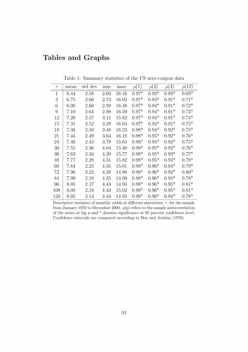
The data is presented in Figure 3. The surface plot illustrates how the yield

curve evolves over time. Table 1 reports the means, standard deviations and

autocorrelations across maturities to further illustrate the properties of the

data.

[TABLE 1 AROUND HERE]

The estimated autocorrelation coefficients are significantly different from zero

at a 95 percent level of confidence for lag one through twelve, across all ma-

8The data can be downloaded from http://www.ssc.upenn.edu/ fdiebold/papers/paper49/FBFITTED.txt and Diebold and Li (2006, pp. 344-345) give a detailed descrip-tion of the data treatment methodology applied.

16

turities.9 Such high autocorrelations could suggest that the underlying yield

series are integrated of order one. If this is the case, we would need to

take first-differences to make the variables stationary before valid statisti-

cal inference could be drawn, or we would have to resort to co-integration

analysis. However, economic theory tells us that nominal yield series cannot

be integrated, since they have a lower bound support at zero and an upper

bound support lower than infinity. Consequently, and in accordance with the

yield-curve literature, we model yields in levels and thus disregard that their

in-sample properties could indicate otherwise.10

III Estimation Procedure

To estimate the Nelson-Siegel factors XNSt in equation (4), we follow Diebold

and Li (2006) by fixing the decay parameter λ = 0.0609 in equation (3) and

by using OLS.11 We treat the obtained Nelson-Siegel factors as observable in

the estimation of the no-arbitrage model presented in equations (7) to (13).

To estimate the parameters of the arbitrage-free model we use the two-step

procedure proposed by Ang et al. (2006). In the first step, we fit a VAR(1)

for the Nelson-Siegel factors to estimate µ, Φ and Σ from equation (11).

And, to estimate the parameters in the short rate equation (13), we project

the short rate (one-month yield) on the Nelson-Siegel yield curve factors. In

9A similar degree of persistence in yield curve data is also noted by Diebold and Li(2006).

10It is often the case in yield-curve modeling that yields are in levels. See, amongothers, Nelson and Siegel (1987), Diebold and Li (2006), Diebold, Rudebusch and Aruoba(2006a), Diebold, Li and Yue (2007), Duffee (2006), Ang and Piazzesi (2003), Bansal andZhou (2002), and Dai and Singleton (2000).

11This value of λ maximizes the loading on the curvature at 30 months maturity asshown by Diebold and Li (2006).

17

the second step, we minimize the sum of squared residuals between observed

yields and fitted yields to estimate the market-price-of-risk parameters λ0

and λ1 of equation (12). Finally, we compute aNA and bNA.

Our goal is to test whether the Nelson-Siegel model in equations (2) to

(4) is statistically different from the no-arbitrage model in equations (7) to

(13). Since the estimated factors, XNSt are the same for both models we can

formulate our hypotheses is the following way:

H10 : aNA

τ = aNSτ ≡ 0,

H20 : bNA

τ (1) = bNSτ (1),

H30 : bNA

τ (2) = bNSτ (2),

H40 : bNA

τ (3) = bNSτ (3),

where bNAτ (k) denotes the loadings on the k-th factor in the no-arbitrage

model at maturity τ , and bNSτ (k) denotes the corresponding variable from

the Nelson-Siegel model.

We claim that the Nelson-Siegel model is compatible with arbitrage-

freeness if H10 to H4

0 are not rejected at traditional levels of confidence.

Notice that to test for H10 to H4

0 we only need to estimate aNA and bNA,

since the Nelson-Siegel loading structure is fixed from the model. To account

for the two-step estimation procedure of the no-arbitrage model and for the

generated regressor problem, we construct confidence intervals around aNA

and bNA using the resampling procedure described in the next section.

18

A Resampling procedure

Bootstrap methods come in many guises in the field of financial econometrics,

see among others Davidson and MacKinnon (2006) for a general overview

with an emphasis on hypothesis testing. There exist three generic forms of

bootstrapping: parametric, semi-parametric and non-parametric. Paramet-

ric bootstrapping refers to a situation where the data generating process can

be written down explicitly, and where the error-term distribution fulfils stan-

dard criteria (Niid). In this case new data samples are generated by drawing

innovations from a normal distribution and feeding them through the true

data generating process. In semi-parametric bootstrapping the distributional

assumption on the error-term made under the parametric setting is relaxed.

Rather it is assumed that errors are iid, but not necessarily normal, in which

case new data samples can be generated by resampling from the empirical

residuals, and feeding the resampled residuals through the data generating

process. A variant of semi-parametric bootstrapping, called (circular) block-

bootstrap, exists to cater for the event where the empirical residuals are

serially autocorrelated. Here ”blocks” of the empirical residuals are drawn

and the blocks are concatenated to form a full-length series of innovations,

which are then fed through the mode. Finally, the non-parametric method

refers to the “original” bootstrap method as suggested by Efron (1979). Fol-

lowing this approach one does not assume a true data generating process,

but instead resamples the observed data.

To recover the empirical distributions of the estimated parameters we con-

duct non-parametric circular block resampling, in the spirit of Efron (1979),

19

and reconstruct multiple yield curve data samples from the original yield

curve data. Alternatively, a semi-parametric bootstrapping technique could

have been applied.12 In principle, our assumed data generating process is

the Nelson-Siegel model, cast in state space form. Hence, the observation

equation is the Nelson-Siegel yield equation (4) and the state equation is a

VAR(1) for the yield curve factors equation (11), which is similar to Diebold

and Li (2006). Residuals are then observable at the level of the state and

the observation equations. It is common that residuals from models apply-

ing yield curve data generate residuals that are strongly autocorrelated.13

Consequently, a semi-parametric block-bootstrapping scheme could be used,

where innovations to the state and observation equations are drawn, whereby

new yield-curve data-samples would be generated. However, it is not clear

what would be gained from using a semi-parametric approach in our setting,

in particular, since we do not focus our hypothesis tests on pivot statistics

but directly on the estimated parameters.14

12A parametric bootstrap is deemed unrealistic in the preset case due to the statisticalproperties of the data.

13Using co-integration analysis, as e.g. Campbell and Shiller (1991) the problem of highresidual autocorellation is naturally removed.

14It seems that bootstrapping pivot statistics, i.e. statistics that do not depend on theparameters of the estimated model, generally provide better statistical results, than whatis obtained when bootstrapping the parameters of the model directly (see e.g. Davidsonand MacKinnon (2006)). It could therefore (possibly) be argued, that a semi-parametricapproach would have the advantage of allowing us to recover the standard errors of theestimated parameters, by calculating the first derivatives to our model, and, as such, allowus to base hypothesis testing on pivot statistics. However, it is not entirely clear how thiswould be done in our two-stage estimation procedure, and further more, acknowledgingthat yield curve data is nearly I(1) series, it seems more than heroic to assume that sucha scheme would provide reliable results. In this connection it should also be mentioned,that a semi-parametric resampling scheme would also imply an explicit assumption tobe made about the correlation structure between innovations to the dynamic evolution ofyield curve factors and the innovations to the yield equation. Such an explicit modelling ofinnovation term correlation is naturally subject to err as regards to the assumptions made.A non-parametric resampling scheme applied directly at the level of observed yields does

20

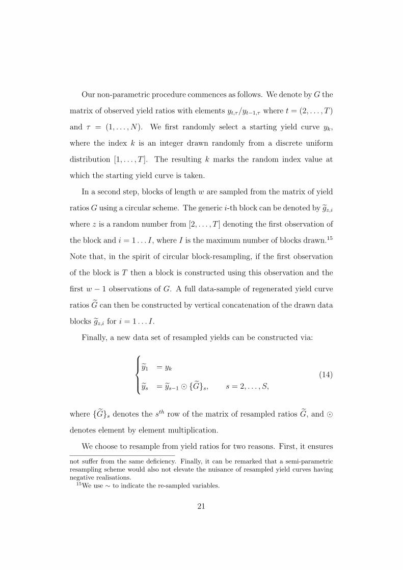
Our non-parametric procedure commences as follows. We denote by G the

matrix of observed yield ratios with elements yt,τ/yt−1,τ where t = (2, . . . , T )

and τ = (1, . . . , N). We first randomly select a starting yield curve yk,

where the index k is an integer drawn randomly from a discrete uniform

distribution [1, . . . , T ]. The resulting k marks the random index value at

which the starting yield curve is taken.

In a second step, blocks of length w are sampled from the matrix of yield

ratios G using a circular scheme. The generic i-th block can be denoted by gz,i

where z is a random number from [2, . . . , T ] denoting the first observation of

the block and i = 1 . . . I, where I is the maximum number of blocks drawn.15

Note that, in the spirit of circular block-resampling, if the first observation

of the block is T then a block is constructed using this observation and the

first w − 1 observations of G. A full data-sample of regenerated yield curve

ratios G can then be constructed by vertical concatenation of the drawn data

blocks gz,i for i = 1 . . . I.

Finally, a new data set of resampled yields can be constructed via:

y1 = yk

ys = ys−1 ¯ Gs, s = 2, . . . , S,

(14)

where Gs denotes the sth row of the matrix of resampled ratios G, and ¯denotes element by element multiplication.

We choose to resample from yield ratios for two reasons. First, it ensures

not suffer from the same deficiency. Finally, it can be remarked that a semi-parametricresampling scheme would also not elevate the nuisance of resampled yield curves havingnegative realisations.

15We use ∼ to indicate the re-sampled variables.

21

positiveness of the resampled yields. Second, as reported in Table 1, yields

are highly autocorrelated and close to I(1). Therefore, one could resample

from first differences, but as reported in Table 2, first differences of yields

are highly autocorrelated and not variance-stationary. Yield ratios display

better statistical properties regarding variance-stationarity, as can be seen

by comparing the correlation coefficients for squared differences and ratios

in Table 2. Block-bootstrapping is used to account for serial correlation

in the yield curve ratios. Moreover, the circular scheme corrects the issue

pertaining to the regular block bootstrap technique of not allocating equal

sampling probability to observations located at the beginning and at the end

of the data series.16

[TABLE 2 AROUND HERE]

A similar resampling technique has been proposed by Rebonato et al.

(2005). They provide a detailed account for the desirable statistical features

of this approach. In the present context we recall that the method ensures: (i)

the exact asymptotic recovery of all the eigenvalues and eigenvectors of yields;

(ii) the correct reproduction of the distribution of curvatures of the yield

16We thank V. Corradi for pointing out to us that resampling from ratios leads ourresampled data to have a biased mean. However, since this bias can be shown to affectresults only when the yield ratios deviate from unity, the bias problem can only marginallyinfluence our results. In fact, the mean of yield ratios across all maturities in our datasample is close to unity; reflecting the near integratedness of yield curve data. In addition,it should be mentioned, that the obvious alternative, namely sampling from the firstdifferences of yields, will also bias the mean of the resampled data. This bias wouldhowever not be introduced at the bootstrapping level, but when enforcing that nominalyields are only meaningful when they are positive. In practice, when resampling fromfirst differences, one would need to discard all yield curve realisations having one or moreresampled yield observations landing in the negative territory. Naturally, such a procedurewould also bias the mean of the resampled series, and the bias would be of an unknownsize.

22

curve across maturities; (iii) the correct qualitative recovery of the transition

from super- to sub-linearity as the yield maturity is increased in the variance

of n-day changes, and (iv) satisfactory accounting of the empirically-observed

positive serial correlations in the yields.

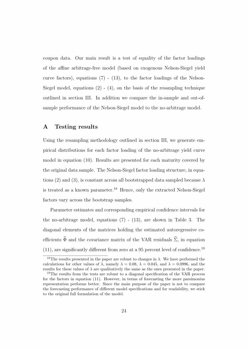
To test hypotheses H10 to H4

0 we employ the following scheme:

(1) Construct a yield curve sample y following equation (14);

(2) Estimate the Nelson-Siegel yield curve factors XNSt on y;

(3) Use XNSt to estimate the parameters aNA and bNA from the arbitrage-

free model given in equations (7) - (13);

(4) Repeat steps 1 to 3, 1000 times to build a distribution for the parameter

estimates aNA and bNA;

(5) Construct confidence intervals for aNA and bNA using the sample quan-

tiles of the empirical distribution of the estimated parameters.

Note that by fixing λ in step 2, the Nelson-Siegel factor loading structure

remains unchanged from repetition to repetition. We set the block length

equal to 48 observations (4 years of data), i.e. w = 48, and generate a total

of 372 yield curve observations for each replication, i.e. S = 372.17

IV Results

This section presents three sets of results to help assess whether the Nelson-

Siegel model is compatible with arbitrage-freeness when applied to US zero-

17All the results presented in the paper are robust to changes in the size of the blocklength (in a reasonable way).

23

coupon data. Our main result is a test of equality of the factor loadings

of the affine arbitrage-free model (based on exogenous Nelson-Siegel yield

curve factors), equations (7) - (13), to the factor loadings of the Nelson-

Siegel model, equations (2) - (4), on the basis of the resampling technique

outlined in section III. In addition we compare the in-sample and out-of-

sample performance of the Nelson-Siegel model to the no-arbitrage model.

A Testing results

Using the resampling methodology outlined in section III, we generate em-

pirical distributions for each factor loading of the no-arbitrage yield curve

model in equation (10). Results are presented for each maturity covered by

the original data sample. The Nelson-Siegel factor loading structure, in equa-

tions (2) and (3), is constant across all bootstrapped data sampled because λ

is treated as a known parameter.18 Hence, only the extracted Nelson-Siegel

factors vary across the bootstrap samples.

Parameter estimates and corresponding empirical confidence intervals for

the no-arbitrage model, equations (7) - (13), are shown in Table 3. The

diagonal elements of the matrices holding the estimated autoregressive co-

efficients Φ and the covariance matrix of the VAR residuals Σ, in equation

(11), are significantly different from zero at a 95 percent level of confidence.19

18The results presented in the paper are robust to changes in λ. We have performed thecalculations for other values of λ, namely λ = 0.08, λ = 0.045, and λ = 0.0996, and theresults for these values of λ are qualitatively the same as the ones presented in the paper.

19The results from the tests are robust to a diagonal specification of the VAR processfor the factors in equation (11). However, in terms of forecasting the more parsimoniusrepresentation performs better. Since the main purpose of the paper is not to comparethe forecasting performance of different model specifications and for readability, we stickto the original full formulation of the model.

24

In addition, the estimates of the first two elements of the (3× 1) vector bNA1

in equation (13), are also different from zero, judged at the same level of con-

fidence. The estimate for aNA1 is not significantly different from zero, which

is in line with the zero intercept in the NS model.

[TABLE 3 AROUND HERE]

The estimated intercepts of the no-arbitrage model aNA, computed as in

equations (7) - (8), are presented in Table 4, for each maturity covered by the

original data. This table reports also the 95 percent confidence intervals, ob-

tained from the resampling, and the Nelson-Siegel intercepts aNS. Therefore,

results in Table 4 allow for testing H10 for the equality between the intercepts

in the yield curve equations for the no-arbitrage and the Nelson-Siegel mod-

els. Tables 5 to 7 present the corresponding results that allow us to test H20 ,

H30 , and H4

0 , i.e. whether the corresponding yield curve factor loadings are

equal. The empirical 95 percent confidence intervals are included in Tables

4, 5, 6 and 7. The upper and lower bounds of the confidence intervals are

denoted by a subscript U L, respectively.

[TABLE 4 to 7 AROUND HERE]

Figure 4 gives a visual representation of the results contained in Tables

4 to 7. The figure shows the estimated no-arbitrage loadings, aNA and bNA,

with the relative 50 percent and 95 percent empirical confidence intervals

obtained from resampling, as well as the parameter values for the Nelson-

Siegel model, i.e. aNS and bNS, for comparison.

25

It is clear from Figure 4 that the empirical distributions are highly skewed

for most of the maturities. Consider, for example, the plot for the intercept

estimates (the top left plot in Figure 4) at maturity 120.

[FIGURE 4 AROUND HERE]

This non-normality of the distributions for the estimated no-arbitrage param-

eters, is further analyzed in Table 8. This table shows that all distributions

display skewness, excess kurtosis, or both. Selected maturities are shown in

Table 8, however, this result holds for all maturities included in the sample.

We also perform the Jarque-Bera test for normality, and reject normality at

a 95 percent confidence level for all maturities.

[TABLE 8 AROUND HERE]

Visual confirmation of the documented non-normality is provided by Figures

5 to 8. For a representative selection of maturities, these figures show the

empirical distribution of the estimated no-arbitrage loadings, and a normal

distribution approximation. In addition, the figures show the 95 percent con-

fidence intervals computed as sample quantiles of the empirical distribution

of the parameters and the normal approximation.

[FIGURE 5 to 8 AROUND HERE]

The non-normality of the empirical distributions for the bootstrapped inter-

cepts aNA, and factor loadings bNA, indicates that the confidence intervals

should be constructed using the sample quantiles of the empirical distribu-

tion.

26

By inspecting the tables, we reach the following conclusions for the tested

hypotheses:

H10 : aNA

τ = aNSτ ≡ 0 not rejected at a 95% level of confidence,

H20 : bNA

τ (1) = bNSτ (1) not rejected at a 95% level of confidence,

H30 : bNA

τ (2) = bNSτ (2) not rejected at a 95% level of confidence,

H40 : bNA

τ (3) = bNSτ (3) not rejected at a 95% level of confidence.

The hypotheses H10 through H4

0 test the equality between each no-arbitrage

factor loading and the corresponding Nelson-Siegel factor loading separately

for each maturity. The last rows of Tables 4 - 7 show the F statistics for

the null hypothesis that the corresponding no-arbitrage factor loadings are

jointly equal to the Nelson-Siegel factor loadings for all maturities in the

sample. To perform these tests we use the empirical variance-covariance

matrix of the estimates obtained from the resampling. All the joint tests

support the result of no statistical difference between the Nelson-Siegel and

the no-arbitrage loadings. We have also computed the joint F test for the

equality of all the NA and NS factor loadings across maturities. The test

statistic is 0.25 and the 95 percent critical F-value with 72 and 300 degrees

of freedom is 1.34. Therefore, we also cannot reject the hypothesis that the

loading structures of the two models are equal.

For the test of the curvature parameter in H40 an additional comment

is warranted. As can be seen from Figure 4, the curvature parameter, at

middle maturities, is the closest to violating the 95 percent confidence band,

and this parameter thus constitutes the “weak point” of the Nelson-Siegel

27

model in relation to the no-arbitrage constraints. This finding is in line with

Bjork and Christensen (1999) who prove that a Nelson-Siegel type model

with two additional curvature factors, each with its own λ, theoretically

would be arbitrage-free. However, when acknowledging that Litterman and

Scheinkman (1991) find that the curvature factor only accounts for approx-

imately 2 percent of the variation of yields, and in the light of our results,

one can question the significance of adding additional factors. Our empiri-

cal finding is also supported by the theoretical results in Christensen et al.

(2007) who show that adding an additional term at very long maturities rec-

onciles the dynamic Nelson-Siegel model with the affine arbitrage-free term

structure models.

Using yield curve modeling for purposes other than relative pricing, as

for example central bankers and fixed-income strategists do, one might be

tempted to use the Nelson-Siegel model on the basis of its compatibility with

arbitrage-freeness.

B In-sample comparison

To conduct an in-sample comparison of the two models, we estimate the

Nelson-Siegel model in equations (2) - (4) and the no-arbitrage model in

equations (7) - (13), where the latter model uses the yield curve factors

extracted from the former. Measures of fit are displayed in Table 9.

A general observation is that both models fit data well: the means of the

residuals for all maturities are close to zero and show low standard devia-

tions. The root mean squared error, RMSE, and the mean absolute deviation,

28

MAD, are also low and similar for both models.

More specifically, Table 9 shows that the averages of the residuals from the

fitted Nelson-Siegel model, εNS, for the included maturities, are all lower than

16 basis points, in absolute value. In fact, the mean of the absolute residuals

across maturities is 5 basis points, while the corresponding number for εNA

is 3 basis points. The 3 months maturity is the worst fitted maturity for the

no-arbitrage model with a mean of the residuals of 8 basis points. For the

Nelson-Siegel model the worst fitted maturity is the 1 month segment with

a mean of the residuals close to -16 bp. Furthermore, the two models have

the same amount of autocorrelation in the residuals. A similar observation

is made for the Nelson-Siegel model alone by Diebold and Li (2006).

[TABLE 9 AROUND HERE]

Drawing a comparison on the basis of RMSE and MAD figures gives the

conclusion that both models fit data equally well.

C Out-of-sample comparison

As a last comparison-check of the equivalence of the Nelson-Siegel model

and the no-arbitrage counterpart, we perform an out-of-sample forecast ex-

periment. In particular, we generate h-steps ahead iterative forecasts in the

following way. First, the yield curve factors are projected forward using the

estimated VAR parameters from equation (11)

XNSt+h|t =

h−1∑s=0

Φsµ + ΦhXNSt ,

29

where h ∈ 1, 6, 12 is the forecasting horizon in months. Second, out-

of-sample forecasts are calculated for the two models, given the projected

factors,

yNSt+h|t = bNSXNS

t+h|t,

yNAt+h|t = aNA

t + bNAt XNS

t+h|t,

where subscripts t on aNAt and aNA

t indicate that parameters are estimated

using data until time t. To evaluate the prediction accuracy at a given

forecasting horizon, we use the mean squared forecast error, MSFE i.e. the

average squared error over the evaluation period, between t0 and t1, for the

h-months ahead forecast of the yield with maturity τ

MSFE(τ, h, m) =1

t1 − t0 + 1

t1∑t=t0

(ym

t+h,τ |t − yt+h,τ

)2, (15)

where m ∈ NA, NS denotes the model.

The results presented are expressed as ratios of the MSFEs of the two

models against the MSFE of a random walk. The random walk represents

a naıve forecasting model that historically has proven very difficult to out-

perform especially at short forecasting horizons. The success of the random

walk model in the area of yield curve forecasting is due to the high degree

of persistence exhibited by observed yields. The random walk h-step ahead

prediction, at time t, of the yield with maturity τ is

yt+h,τ |t = yt,τ .

30

To produce the first set of forecasts, the model parameters are estimated

on a sample defined from 1970:01 to 1993:01, and yields are forecasted for the

chosen horizons, h. The data sample is then increased by one month and the

parameters are re-estimated on the new data covering 1970:01 to 1993:02.

Again, forecasts are produced for the forecasting horizons. This procedure is

repeated for the full sample, generating forecasts on successively increasing

data samples. The forecasting performances are then evaluated over the

period 1994:01 to 2000:12 using the MSFE, as shown in equation (15).

Table 10 reports on the out-of-sample forecast performance of the Nelson-

Siegel and the no-arbitrage model evaluated against the random walk fore-

casts.

[TABLE 10 AROUND HERE]

The well-known phenomenon of the good forecasting performance of the

random walk model is observed for the 1 month forecasting horizon. For the

6 and 12 month forecasting horizons, the Nelson-Siegel model and the no-

arbitrage counterpart generally perform better than the random walk model,

as shown by all ratios being less than one (except for the 10 years maturity).

Turning now to the relative comparison of the no-arbitrage model against

the Nelson-Siegel model, it can be concluded that they exhibit very similar

forecasting performances. If we consider every maturity for each forecasting

horizon as an individual observation, then there are in total 54 observations.

In 24 of these cases the Nelson-Siegel model is better, in 23 cases the no-

arbitrage model is better, and in the remaining 7 cases the models perform

equally well. Even when one model is judged to be better than its competitor,

31

the differences in the performance ratios are very small.

In summary, it can be concluded that there is no systematic pattern across

maturities and forecasting horizons showing when one model is better than

its competitor. Indeed, to formally compare the forecasting performance of

the two models we compute the Diebold-Mariano statistic for each maturity

and forecasting horizon. At a 5 percent level we do not reject the hypothesis

that the no-arbitrage model and the Nelson-Siegel model forecast equally

well for the majority of the forecasts. At this significance level we reject the

hypothesis of equal forecasting performance for maturities 9 and 120 months

in 1-step ahead forecasts and for maturity 96 months in 6- and 12-steps

ahead forecasts. In these four cases the Diebold-Mariano tests shows that

the forecasts produced by the Nelson-Siegel model are better at 5 percent

level of significance. However, none of the models is able to outperform the

other in any maturity for a significance level of 1 percent.

V Conclusion

In this paper we show that the model proposed by Nelson and Siegel (1987) is

compatible with arbitrage-freeness, in the sense that the factor loadings from

the model are not statistically different from those derived from an arbitrage-

free model which uses the Nelson-Siegel factors as exogenous factors, at a 95

percent level of confidence.

In theory, the Nelson-Siegel model is not arbitrage-free as shown by Bjork

and Christensen (1999). However, using US zero-coupon data from 1970 to

2000, a yield curve bootstrapping approach and the implied arbitrage-free

32

factor loadings, we cannot reject the hypothesis that Nelson-Siegel factor

loadings fulfill the no-arbitrage constraints, at a 95 percent confidence level.

Furthermore, we show that the Nelson-Siegel model performs as well as the

no-arbitrage counterpart in an out-of-sample forecasting experiment. Based

on these results, we conclude that the Nelson-Siegel model is compatible with

arbitrage-freeness. This finding implies that the factor loading structure of

the Nelson-Siegel model is rich enough to capture the dynamic behavior of

yield curve factors, when such factors are estimated on data generated by

traders who rely on arbitrage-free models, as it is likely to be the case for

US yield curve data. It is an interesting question whether our suggested

methodology would lead to a rejection of the tested hypothesis if applied to

a less well-organized bond market. We leave this question to be answered by

future research.

Our conclusion is of relevance to fixed-income money managers and cen-

tral banks in particular, since such organizations traditionally rely heavily

on the Nelson-Siegel model for policy and strategic investment decisions.

33

Tables and Graphs

Table 1: Summary statistics of the US zero-coupon data

τ mean std dev min max ρ(1) ρ(2) ρ(3) ρ(12)

1 6.44 2.58 2.69 16.16 0.97* 0.93* 0.89* 0.69*3 6.75 2.66 2.73 16.02 0.97* 0.94* 0.91* 0.71*6 6.98 2.66 2.89 16.48 0.97* 0.94* 0.91* 0.73*9 7.10 2.64 2.98 16.39 0.97* 0.94* 0.91* 0.73*12 7.20 2.57 3.11 15.82 0.97* 0.94* 0.91* 0.74*15 7.31 2.52 3.29 16.04 0.97* 0.94* 0.91* 0.75*18 7.38 2.50 3.48 16.23 0.98* 0.94* 0.92* 0.75*21 7.44 2.49 3.64 16.18 0.98* 0.95* 0.92* 0.76*24 7.46 2.44 3.78 15.65 0.98* 0.94* 0.92* 0.75*30 7.55 2.36 4.04 15.40 0.98* 0.95* 0.92* 0.76*36 7.63 2.34 4.20 15.77 0.98* 0.95* 0.93* 0.77*48 7.77 2.28 4.31 15.82 0.98* 0.95* 0.93* 0.78*60 7.84 2.25 4.35 15.01 0.98* 0.96* 0.94* 0.79*72 7.96 2.22 4.38 14.98 0.98* 0.96* 0.94* 0.80*84 7.99 2.18 4.35 14.98 0.98* 0.96* 0.94* 0.78*96 8.05 2.17 4.43 14.94 0.98* 0.96* 0.95* 0.81*108 8.08 2.18 4.43 15.02 0.98* 0.96* 0.95* 0.81*120 8.05 2.14 4.44 14.93 0.98* 0.96* 0.94* 0.78*Descriptive statistics of monthly yields at different maturities, τ , for the samplefrom January 1970 to December 2000. ρ(p) refers to the sample autocorrelationof the series at lag p and * denotes significance at 95 percent confidence level.Confidence intervals are computed according to Box and Jenkins (1976).

34

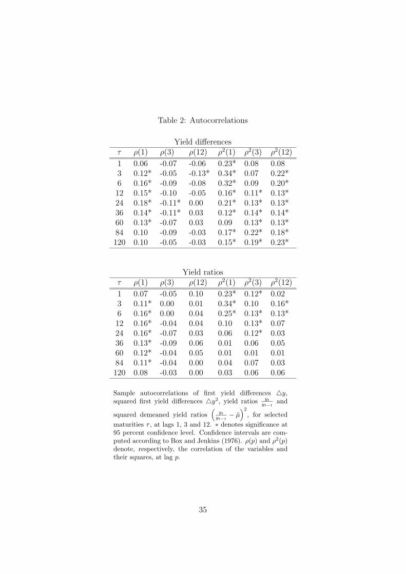
Table 2: Autocorrelations

Yield differencesτ ρ(1) ρ(3) ρ(12) ρ2(1) ρ2(3) ρ2(12)

1 0.06 -0.07 -0.06 0.23* 0.08 0.083 0.12* -0.05 -0.13* 0.34* 0.07 0.22*6 0.16* -0.09 -0.08 0.32* 0.09 0.20*12 0.15* -0.10 -0.05 0.16* 0.11* 0.13*24 0.18* -0.11* 0.00 0.21* 0.13* 0.13*36 0.14* -0.11* 0.03 0.12* 0.14* 0.14*60 0.13* -0.07 0.03 0.09 0.13* 0.13*84 0.10 -0.09 -0.03 0.17* 0.22* 0.18*120 0.10 -0.05 -0.03 0.15* 0.19* 0.23*

Yield ratiosτ ρ(1) ρ(3) ρ(12) ρ2(1) ρ2(3) ρ2(12)

1 0.07 -0.05 0.10 0.23* 0.12* 0.023 0.11* 0.00 0.01 0.34* 0.10 0.16*6 0.16* 0.00 0.04 0.25* 0.13* 0.13*12 0.16* -0.04 0.04 0.10 0.13* 0.0724 0.16* -0.07 0.03 0.06 0.12* 0.0336 0.13* -0.09 0.06 0.01 0.06 0.0560 0.12* -0.04 0.05 0.01 0.01 0.0184 0.11* -0.04 0.00 0.04 0.07 0.03120 0.08 -0.03 0.00 0.03 0.06 0.06

Sample autocorrelations of first yield differences 4y,squared first yield differences 4y2, yield ratios yt

yt−1and

squared demeaned yield ratios(

yt

yt−1− µ

)2

, for selectedmaturities τ , at lags 1, 3 and 12. ∗ denotes significance at95 percent confidence level. Confidence intervals are com-puted according to Box and Jenkins (1976). ρ(p) and ρ2(p)denote, respectively, the correlation of the variables andtheir squares, at lag p.

35

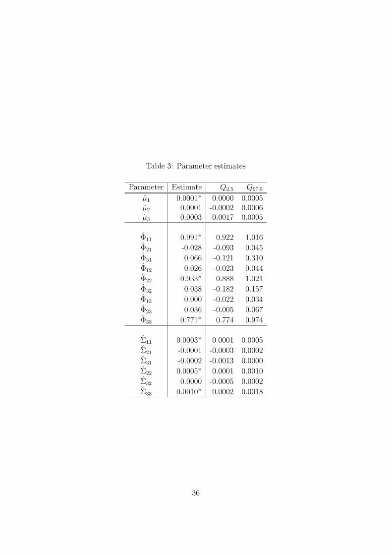
Table 3: Parameter estimates

Parameter Estimate Q2.5 Q97.5

µ1 0.0001* 0.0000 0.0005µ2 0.0001 -0.0002 0.0006µ3 -0.0003 -0.0017 0.0005

Φ11 0.991* 0.922 1.016

Φ21 -0.028 -0.093 0.045

Φ31 0.066 -0.121 0.310

Φ12 0.026 -0.023 0.044

Φ22 0.933* 0.888 1.021

Φ32 0.038 -0.182 0.157

Φ13 0.000 -0.022 0.034

Φ23 0.036 -0.005 0.067

Φ33 0.771* 0.774 0.974

Σ11 0.0003* 0.0001 0.0005

Σ21 -0.0001 -0.0003 0.0002

Σ31 -0.0002 -0.0013 0.0000

Σ22 0.0005* 0.0001 0.0010

Σ32 0.0000 -0.0005 0.0002

Σ33 0.0010* 0.0002 0.0018

36

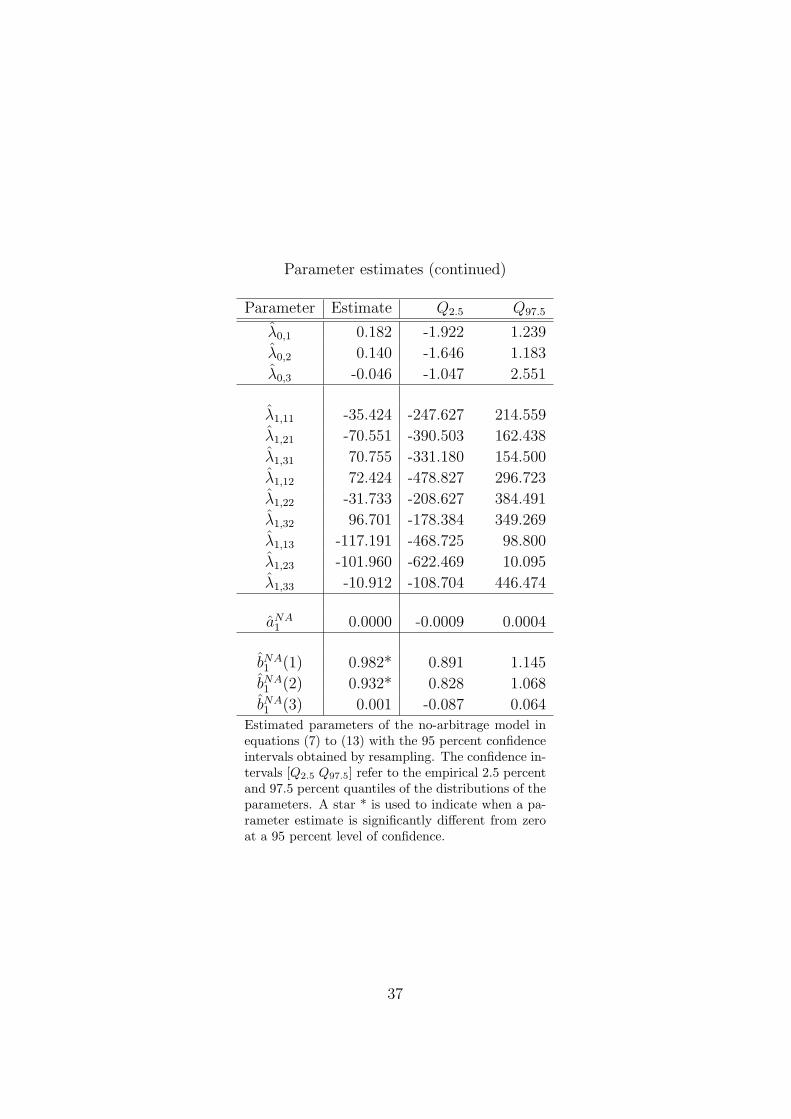
Parameter estimates (continued)

Parameter Estimate Q2.5 Q97.5

λ0,1 0.182 -1.922 1.239

λ0,2 0.140 -1.646 1.183

λ0,3 -0.046 -1.047 2.551

λ1,11 -35.424 -247.627 214.559

λ1,21 -70.551 -390.503 162.438

λ1,31 70.755 -331.180 154.500

λ1,12 72.424 -478.827 296.723

λ1,22 -31.733 -208.627 384.491

λ1,32 96.701 -178.384 349.269

λ1,13 -117.191 -468.725 98.800

λ1,23 -101.960 -622.469 10.095

λ1,33 -10.912 -108.704 446.474

aNA1 0.0000 -0.0009 0.0004

bNA1 (1) 0.982* 0.891 1.145

bNA1 (2) 0.932* 0.828 1.068

bNA1 (3) 0.001 -0.087 0.064

Estimated parameters of the no-arbitrage model inequations (7) to (13) with the 95 percent confidenceintervals obtained by resampling. The confidence in-tervals [Q2.5 Q97.5] refer to the empirical 2.5 percentand 97.5 percent quantiles of the distributions of theparameters. A star * is used to indicate when a pa-rameter estimate is significantly different from zeroat a 95 percent level of confidence.

37

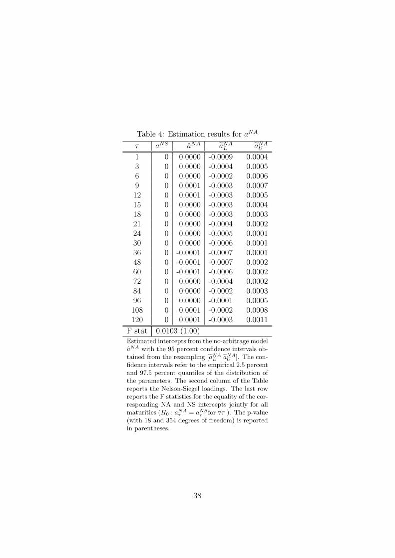
Table 4: Estimation results for aNA

τ aNS aNA aNAL aNA

U

1 0 0.0000 -0.0009 0.00043 0 0.0000 -0.0004 0.00056 0 0.0000 -0.0002 0.00069 0 0.0001 -0.0003 0.000712 0 0.0001 -0.0003 0.000515 0 0.0000 -0.0003 0.000418 0 0.0000 -0.0003 0.000321 0 0.0000 -0.0004 0.000224 0 0.0000 -0.0005 0.000130 0 0.0000 -0.0006 0.000136 0 -0.0001 -0.0007 0.000148 0 -0.0001 -0.0007 0.000260 0 -0.0001 -0.0006 0.000272 0 0.0000 -0.0004 0.000284 0 0.0000 -0.0002 0.000396 0 0.0000 -0.0001 0.0005108 0 0.0001 -0.0002 0.0008120 0 0.0001 -0.0003 0.0011

F stat 0.0103 (1.00)Estimated intercepts from the no-arbitrage modelaNA with the 95 percent confidence intervals ob-tained from the resampling [aNA

L aNAU ]. The con-

fidence intervals refer to the empirical 2.5 percentand 97.5 percent quantiles of the distribution ofthe parameters. The second column of the Tablereports the Nelson-Siegel loadings. The last rowreports the F statistics for the equality of the cor-responding NA and NS intercepts jointly for allmaturities (H0 : aNA

τ = aNSτ for ∀τ ). The p-value

(with 18 and 354 degrees of freedom) is reportedin parentheses.

38

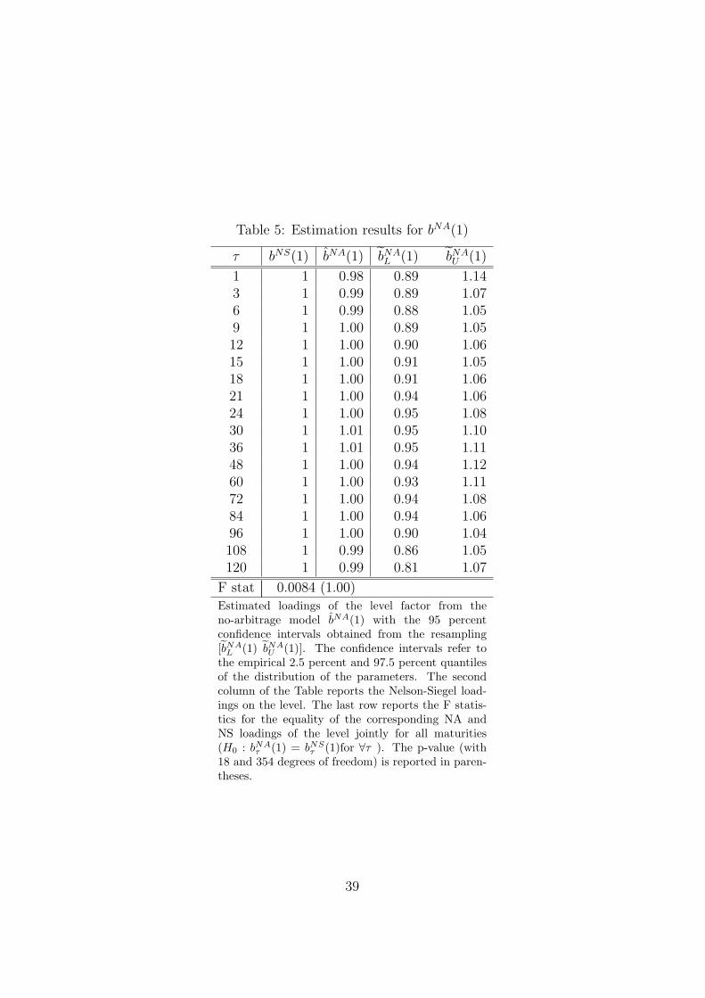
Table 5: Estimation results for bNA(1)

τ bNS(1) bNA(1) bNAL (1) bNA

U (1)

1 1 0.98 0.89 1.143 1 0.99 0.89 1.076 1 0.99 0.88 1.059 1 1.00 0.89 1.0512 1 1.00 0.90 1.0615 1 1.00 0.91 1.0518 1 1.00 0.91 1.0621 1 1.00 0.94 1.0624 1 1.00 0.95 1.0830 1 1.01 0.95 1.1036 1 1.01 0.95 1.1148 1 1.00 0.94 1.1260 1 1.00 0.93 1.1172 1 1.00 0.94 1.0884 1 1.00 0.94 1.0696 1 1.00 0.90 1.04108 1 0.99 0.86 1.05120 1 0.99 0.81 1.07

F stat 0.0084 (1.00)Estimated loadings of the level factor from theno-arbitrage model bNA(1) with the 95 percentconfidence intervals obtained from the resampling[bNA

L (1) bNAU (1)]. The confidence intervals refer to

the empirical 2.5 percent and 97.5 percent quantilesof the distribution of the parameters. The secondcolumn of the Table reports the Nelson-Siegel load-ings on the level. The last row reports the F statis-tics for the equality of the corresponding NA andNS loadings of the level jointly for all maturities(H0 : bNA

τ (1) = bNSτ (1)for ∀τ ). The p-value (with

18 and 354 degrees of freedom) is reported in paren-theses.

39

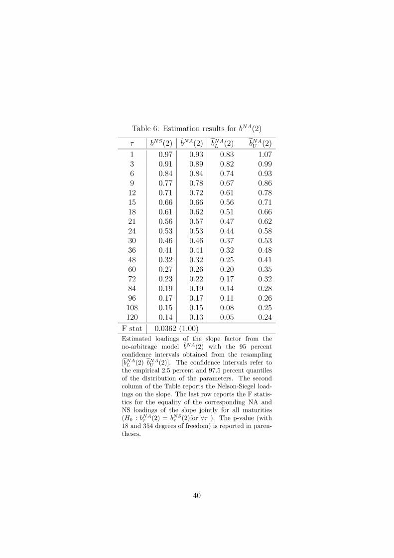
Table 6: Estimation results for bNA(2)

τ bNS(2) bNA(2) bNAL (2) bNA

U (2)

1 0.97 0.93 0.83 1.073 0.91 0.89 0.82 0.996 0.84 0.84 0.74 0.939 0.77 0.78 0.67 0.8612 0.71 0.72 0.61 0.7815 0.66 0.66 0.56 0.7118 0.61 0.62 0.51 0.6621 0.56 0.57 0.47 0.6224 0.53 0.53 0.44 0.5830 0.46 0.46 0.37 0.5336 0.41 0.41 0.32 0.4848 0.32 0.32 0.25 0.4160 0.27 0.26 0.20 0.3572 0.23 0.22 0.17 0.3284 0.19 0.19 0.14 0.2896 0.17 0.17 0.11 0.26108 0.15 0.15 0.08 0.25120 0.14 0.13 0.05 0.24

F stat 0.0362 (1.00)Estimated loadings of the slope factor from theno-arbitrage model bNA(2) with the 95 percentconfidence intervals obtained from the resampling[bNA

L (2) bNAU (2)]. The confidence intervals refer to

the empirical 2.5 percent and 97.5 percent quantilesof the distribution of the parameters. The secondcolumn of the Table reports the Nelson-Siegel load-ings on the slope. The last row reports the F statis-tics for the equality of the corresponding NA andNS loadings of the slope jointly for all maturities(H0 : bNA

τ (2) = bNSτ (2)for ∀τ ). The p-value (with

18 and 354 degrees of freedom) is reported in paren-theses.

40

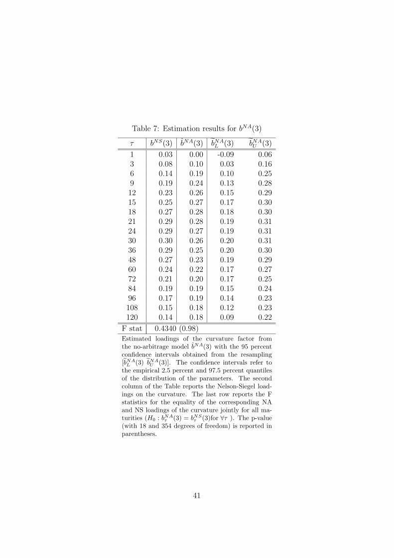
Table 7: Estimation results for bNA(3)

τ bNS(3) bNA(3) bNAL (3) bNA

U (3)

1 0.03 0.00 -0.09 0.063 0.08 0.10 0.03 0.166 0.14 0.19 0.10 0.259 0.19 0.24 0.13 0.2812 0.23 0.26 0.15 0.2915 0.25 0.27 0.17 0.3018 0.27 0.28 0.18 0.3021 0.29 0.28 0.19 0.3124 0.29 0.27 0.19 0.3130 0.30 0.26 0.20 0.3136 0.29 0.25 0.20 0.3048 0.27 0.23 0.19 0.2960 0.24 0.22 0.17 0.2772 0.21 0.20 0.17 0.2584 0.19 0.19 0.15 0.2496 0.17 0.19 0.14 0.23108 0.15 0.18 0.12 0.23120 0.14 0.18 0.09 0.22

F stat 0.4340 (0.98)Estimated loadings of the curvature factor fromthe no-arbitrage model bNA(3) with the 95 percentconfidence intervals obtained from the resampling[bNA

L (3) bNAU (3)]. The confidence intervals refer to

the empirical 2.5 percent and 97.5 percent quantilesof the distribution of the parameters. The secondcolumn of the Table reports the Nelson-Siegel load-ings on the curvature. The last row reports the Fstatistics for the equality of the corresponding NAand NS loadings of the curvature jointly for all ma-turities (H0 : bNA

τ (3) = bNSτ (3)for ∀τ ). The p-value

(with 18 and 354 degrees of freedom) is reported inparentheses.

41

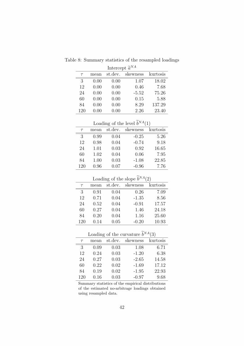
Table 8: Summary statistics of the resampled loadings

Intercept aNA

τ mean st.dev. skewness kurtosis

3 0.00 0.00 1.07 18.0212 0.00 0.00 0.46 7.6824 0.00 0.00 -5.52 75.2660 0.00 0.00 0.15 5.8884 0.00 0.00 8.29 137.29120 0.00 0.00 2.26 23.40

Loading of the level bNA(1)τ mean st.dev. skewness kurtosis

3 0.99 0.04 -0.25 5.2612 0.98 0.04 -0.74 9.1824 1.01 0.03 0.92 16.6560 1.02 0.04 0.06 7.9584 1.00 0.03 -1.08 22.85120 0.96 0.07 -0.96 7.76

Loading of the slope bNA(2)τ mean st.dev. skewness kurtosis

3 0.91 0.04 0.26 7.0912 0.71 0.04 -1.35 8.5624 0.52 0.04 -0.91 17.5760 0.27 0.04 1.46 24.1884 0.20 0.04 1.16 25.60120 0.14 0.05 -0.20 10.93

Loading of the curvature bNA(3)τ mean st.dev. skewness kurtosis

3 0.09 0.03 1.08 6.7112 0.24 0.03 -1.20 6.3824 0.27 0.03 -2.65 14.5860 0.22 0.02 -1.69 17.1284 0.19 0.02 -1.95 22.93120 0.16 0.03 -0.97 9.68Summary statistics of the empirical distributionsof the estimated no-arbitrage loadings obtainedusing resampled data.

42

Table 9: Measures of Fit

Residuals from the Nelson-Siegel modelτ mean st dev min max RMSE MAD ρ(1) ρ(6) ρ(12)

1 -0.159 0.200 -1.046 0.387 0.200 0.040 0.513 0.332 0.4433 0.027 0.114 -0.496 0.584 0.114 0.013 0.274 0.159 0.3266 0.091 0.135 -0.412 0.680 0.135 0.018 0.543 0.346 0.47112 0.046 0.122 -0.279 0.483 0.122 0.015 0.586 0.127 0.28924 -0.040 0.073 -0.398 0.261 0.073 0.005 0.493 0.044 0.15336 -0.066 0.090 -0.432 0.339 0.089 0.008 0.417 0.256 0.18360 -0.053 0.096 -0.520 0.292 0.096 0.009 0.655 0.312 -0.03784 0.006 0.097 -0.446 0.337 0.096 0.009 0.518 0.159 -0.083120 0.002 0.140 -0.763 0.436 0.140 0.020 0.699 0.345 0.091

Residuals from no-arbitrage modelτ Mean st dev min max RMSE MAD ρ(1) ρ(6) ρ(12)

1 0.000 0.168 -0.730 0.752 0.168 0.028 0.361 0.197 0.3633 0.079 0.132 -0.512 0.815 0.132 0.018 0.448 0.218 0.3116 0.058 0.134 -0.299 0.792 0.134 0.018 0.577 0.359 0.43012 -0.019 0.109 -0.357 0.436 0.109 0.012 0.512 0.144 0.30424 -0.040 0.072 -0.322 0.217 0.072 0.005 0.494 0.138 0.09436 -0.017 0.089 -0.286 0.405 0.088 0.008 0.478 0.322 0.26460 0.003 0.100 -0.332 0.378 0.100 0.010 0.687 0.350 0.09984 0.019 0.097 -0.486 0.342 0.097 0.010 0.529 0.157 -0.068120 -0.059 0.144 -0.798 0.380 0.144 0.021 0.706 0.466 0.251

Summary statistics of residuals of the Nelson-Siegel and the no-arbitrage models. TheNelson-Siegel model is estimated according to equations (2) - (4). The no-arbitrage yieldcurve model is estimated according to equations (7) - (13). Statistics are shown forselected maturities, τ . RMSE is the root mean squared error and MAD is the meanabsolute deviation. Autocorrelations are denoted by ρ(p), where p is the lag.

43

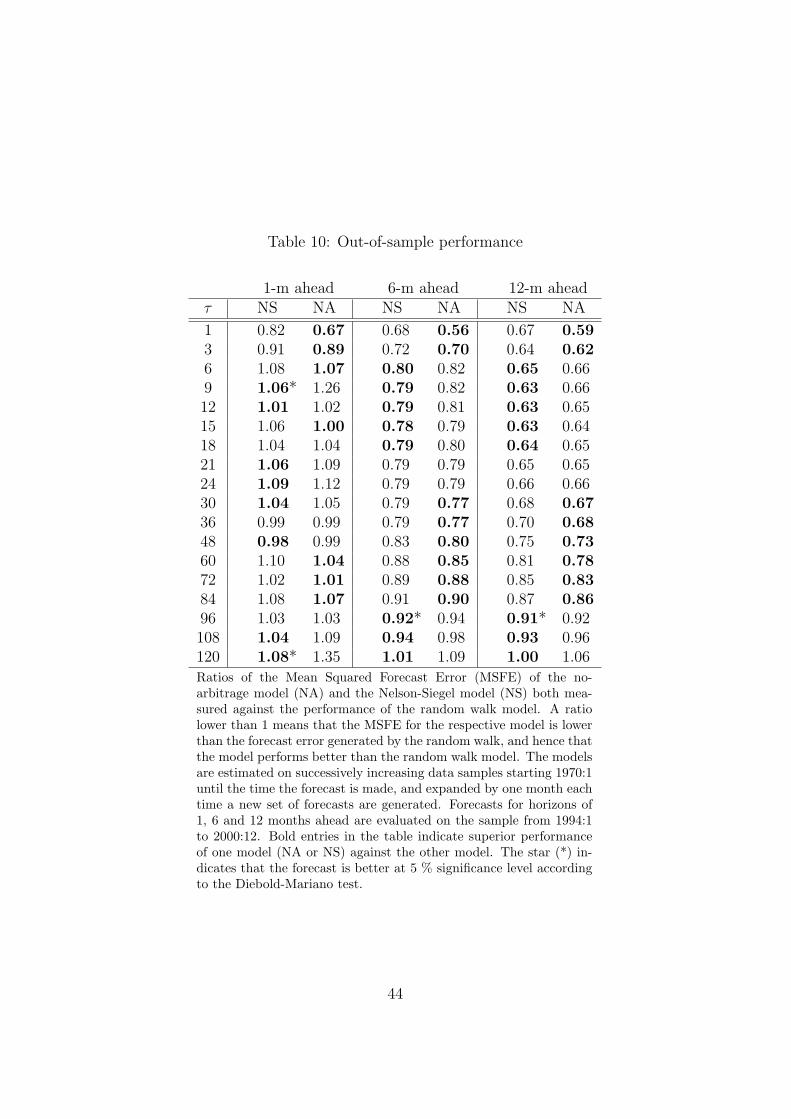
Table 10: Out-of-sample performance

1-m ahead 6-m ahead 12-m aheadτ NS NA NS NA NS NA

1 0.82 0.67 0.68 0.56 0.67 0.593 0.91 0.89 0.72 0.70 0.64 0.626 1.08 1.07 0.80 0.82 0.65 0.669 1.06* 1.26 0.79 0.82 0.63 0.6612 1.01 1.02 0.79 0.81 0.63 0.6515 1.06 1.00 0.78 0.79 0.63 0.6418 1.04 1.04 0.79 0.80 0.64 0.6521 1.06 1.09 0.79 0.79 0.65 0.6524 1.09 1.12 0.79 0.79 0.66 0.6630 1.04 1.05 0.79 0.77 0.68 0.6736 0.99 0.99 0.79 0.77 0.70 0.6848 0.98 0.99 0.83 0.80 0.75 0.7360 1.10 1.04 0.88 0.85 0.81 0.7872 1.02 1.01 0.89 0.88 0.85 0.8384 1.08 1.07 0.91 0.90 0.87 0.8696 1.03 1.03 0.92* 0.94 0.91* 0.92108 1.04 1.09 0.94 0.98 0.93 0.96120 1.08* 1.35 1.01 1.09 1.00 1.06Ratios of the Mean Squared Forecast Error (MSFE) of the no-arbitrage model (NA) and the Nelson-Siegel model (NS) both mea-sured against the performance of the random walk model. A ratiolower than 1 means that the MSFE for the respective model is lowerthan the forecast error generated by the random walk, and hence thatthe model performs better than the random walk model. The modelsare estimated on successively increasing data samples starting 1970:1until the time the forecast is made, and expanded by one month eachtime a new set of forecasts are generated. Forecasts for horizons of1, 6 and 12 months ahead are evaluated on the sample from 1994:1to 2000:12. Bold entries in the table indicate superior performanceof one model (NA or NS) against the other model. The star (*) in-dicates that the forecast is better at 5 % significance level accordingto the Diebold-Mariano test.

44

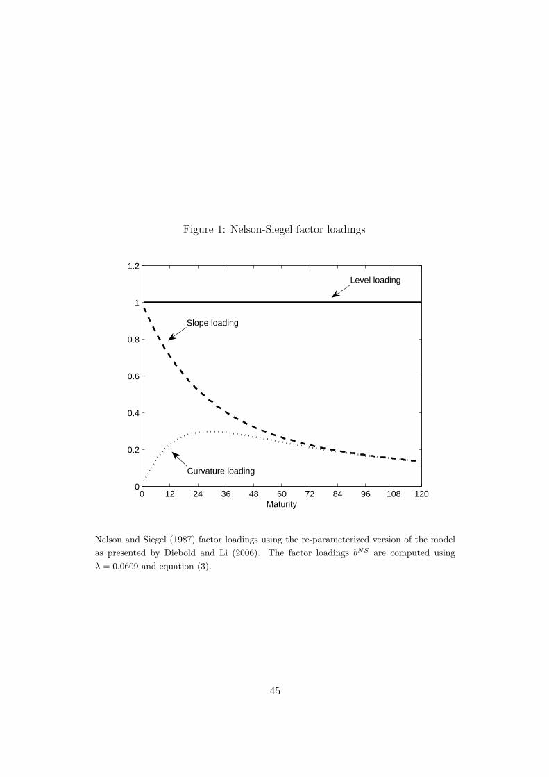
Figure 1: Nelson-Siegel factor loadings

0 12 24 36 48 60 72 84 96 108 1200

0.2

0.4

0.6

0.8

1

1.2

Maturity

Level loading

Slope loading

Curvature loading

Nelson and Siegel (1987) factor loadings using the re-parameterized version of the modelas presented by Diebold and Li (2006). The factor loadings bNS are computed usingλ = 0.0609 and equation (3).

45

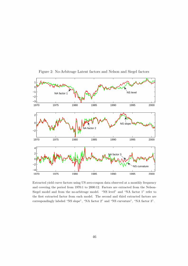
Figure 2: No-Arbitrage Latent factors and Nelson and Siegel factors

1970 1975 1980 1985 1990 1995 2000−3

−2

−1

0

1

1970 1975 1980 1985 1990 1995 2000

−2

0

2

1970 1975 1980 1985 1990 1995 2000

−4

−2

0

2

4

NS levelNA factor 1

NS slope

NA factor 2

NS curvature

NA factor 3

Extracted yield curve factors using US zero-coupon data observed at a monthly frequencyand covering the period from 1970:1 to 2000:12. Factors are extracted from the Nelson-Siegel model and from the no-arbitrage model. “NS level” and “NA factor 1” refer tothe first extracted factor from each model. The second and third extracted factors arecorrespondingly labeled “NS slope”, “NA factor 2” and “NS curvature”, “NA factor 3”.

46

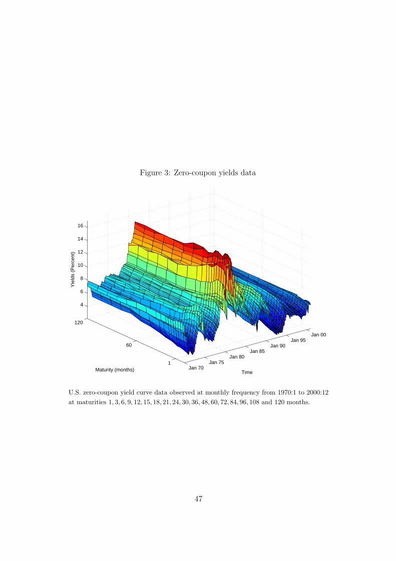
Figure 3: Zero-coupon yields data

Jan 70Jan 75

Jan 80Jan 85

Jan 90Jan 95

Jan 00

1

60

120

4

6

8

10

12

14

16

TimeMaturity (months)

Yie

lds

(Per

cent

)

U.S. zero-coupon yield curve data observed at monthly frequency from 1970:1 to 2000:12at maturities 1, 3, 6, 9, 12, 15, 18, 21, 24, 30, 36, 48, 60, 72, 84, 96, 108 and 120 months.

47

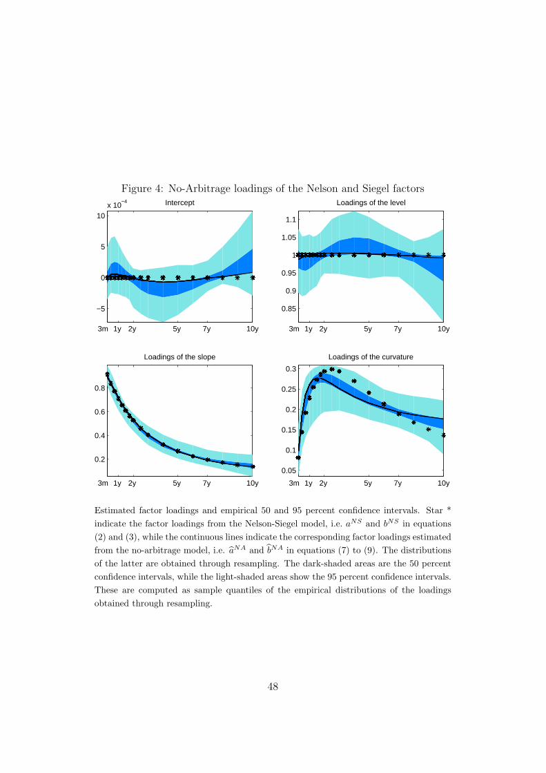
Figure 4: No-Arbitrage loadings of the Nelson and Siegel factors

3m 1y 2y 5y 7y 10y

−5

0

5

10x 10

−4 Intercept

3m 1y 2y 5y 7y 10y

0.85

0.9

0.95

1

1.05

1.1

Loadings of the level

3m 1y 2y 5y 7y 10y

0.2

0.4

0.6

0.8

Loadings of the slope

3m 1y 2y 5y 7y 10y

0.05

0.1

0.15

0.2

0.25

0.3

Loadings of the curvature

Estimated factor loadings and empirical 50 and 95 percent confidence intervals. Star *indicate the factor loadings from the Nelson-Siegel model, i.e. aNS and bNS in equations(2) and (3), while the continuous lines indicate the corresponding factor loadings estimatedfrom the no-arbitrage model, i.e. aNA and bNA in equations (7) to (9). The distributionsof the latter are obtained through resampling. The dark-shaded areas are the 50 percentconfidence intervals, while the light-shaded areas show the 95 percent confidence intervals.These are computed as sample quantiles of the empirical distributions of the loadingsobtained through resampling.

48

Figure 5: Distribution of the estimated loadings for aNA

−1 0 1 2

x 10−3

500

1000

1500

2000

2500

Intercept, maturity 3

−1 −0.5 0 0.5 1 1.5

x 10−3

500

1000

1500

2000

2500Intercept, maturity 12

−1 −0.5 0 0.5 1

x 10−3

500

1000

1500

2000

Intercept, maturity 60

−1 0 1 2 3 4

x 10−3

200

400

600

800

1000

1200

Intercept, maturity 120

Empirical distributions, for selected maturities, of the no-arbitrage intercepts obtainedfrom the resampling (continuous line), with the relative 95 percent confidence interval(asterisks) computed as sample quantiles. The dashed line is the Gaussian approximationwith the relative 95 percent confidence intervals (circles). The diamonds are the esti-mated no-arbitrage intercepts and the dashed vertical line indicates the Nelson and Siegelintercepts.

49

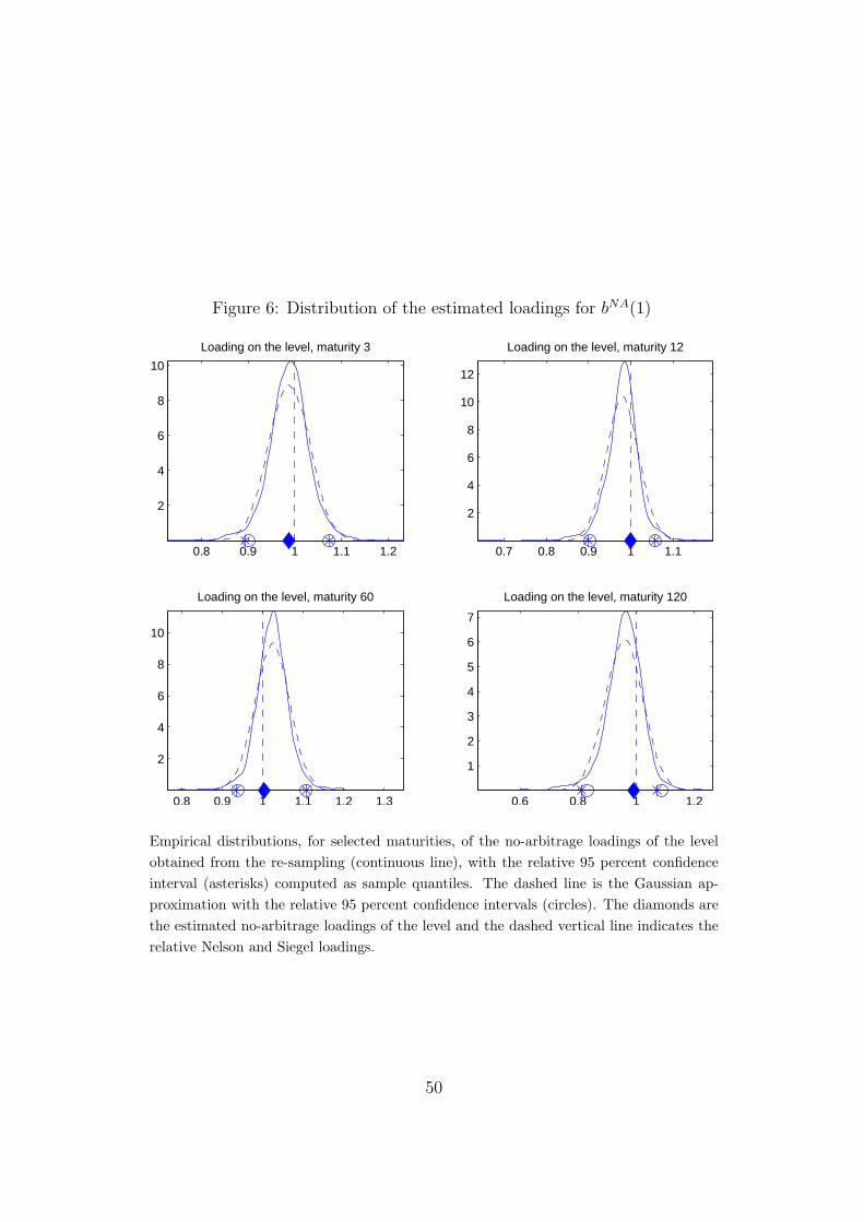
Figure 6: Distribution of the estimated loadings for bNA(1)

0.8 0.9 1 1.1 1.2

2

4

6

8

10

Loading on the level, maturity 3

0.7 0.8 0.9 1 1.1

2

4

6

8

10

12

Loading on the level, maturity 12

0.8 0.9 1 1.1 1.2 1.3

2

4

6

8

10

Loading on the level, maturity 60

0.6 0.8 1 1.2

1

2

3

4

5

6

7

Loading on the level, maturity 120

Empirical distributions, for selected maturities, of the no-arbitrage loadings of the levelobtained from the re-sampling (continuous line), with the relative 95 percent confidenceinterval (asterisks) computed as sample quantiles. The dashed line is the Gaussian ap-proximation with the relative 95 percent confidence intervals (circles). The diamonds arethe estimated no-arbitrage loadings of the level and the dashed vertical line indicates therelative Nelson and Siegel loadings.

50

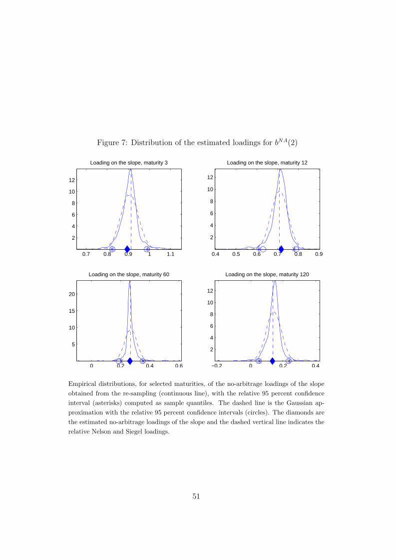
Figure 7: Distribution of the estimated loadings for bNA(2)

0.7 0.8 0.9 1 1.1

2

4

6

8

10

12

Loading on the slope, maturity 3

0.4 0.5 0.6 0.7 0.8 0.9

2

4

6

8

10

12

Loading on the slope, maturity 12

0 0.2 0.4 0.6

5

10

15

20

Loading on the slope, maturity 60

−0.2 0 0.2 0.4

2

4

6

8

10

12

Loading on the slope, maturity 120

Empirical distributions, for selected maturities, of the no-arbitrage loadings of the slopeobtained from the re-sampling (continuous line), with the relative 95 percent confidenceinterval (asterisks) computed as sample quantiles. The dashed line is the Gaussian ap-proximation with the relative 95 percent confidence intervals (circles). The diamonds arethe estimated no-arbitrage loadings of the slope and the dashed vertical line indicates therelative Nelson and Siegel loadings.

51

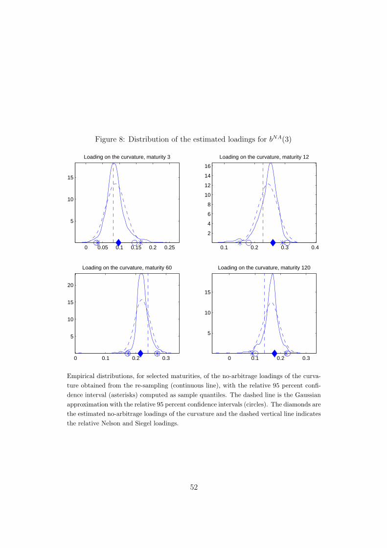
Figure 8: Distribution of the estimated loadings for bNA(3)

0 0.05 0.1 0.15 0.2 0.25

5

10

15

Loading on the curvature, maturity 3

0.1 0.2 0.3 0.4

2

4

6

8

10

12

14

16

Loading on the curvature, maturity 12

0 0.1 0.2 0.3

5

10

15

20

Loading on the curvature, maturity 60

0 0.1 0.2 0.3

5

10

15

Loading on the curvature, maturity 120

Empirical distributions, for selected maturities, of the no-arbitrage loadings of the curva-ture obtained from the re-sampling (continuous line), with the relative 95 percent confi-dence interval (asterisks) computed as sample quantiles. The dashed line is the Gaussianapproximation with the relative 95 percent confidence intervals (circles). The diamonds arethe estimated no-arbitrage loadings of the curvature and the dashed vertical line indicatesthe relative Nelson and Siegel loadings.

52

References

Ahn, Dong-Hyun, Robert F. Dittmar, and Ronald A. Gallant (2002)‘Quadratic Term Structure Models: Theory and Evidence.’ Review ofFinancial Studies 15(1), 243–288

Ang, A., and M. Piazzesi (2003) ‘A No-Arbitrage Vector Autoregression ofTerm Structure Dynamics with Macroeconomic and Latent Variables.’Journal of Monetary Economics 50(4), 745–787

Ang, A., G. Bekaert, and M. Wei (2007) ‘The term structure of real ratesand expected inflation.’ Journal of Finance, forthcoming

Ang, A., M. Piazzesi, and M. Wei (2006) ‘What Does the Yield Curve Tellus about GDP Growth.’ Journal of Econometrics 131, 359–403

Bansal, R., and H. Zhou (2002) ‘Term Structure of Interest Rates withRegime Shifts.’ Journal of Finance 57, 1997–2043

Bernadell, C., J. Coche, and K. Nyholm (2005) ‘Yield Curve Prediction forthe Strategic Investor.’ ECB Working Paper 472

BIS (2005) Zero-Coupon Yield Curves: Technical Documentation (Bank forInternational Settlements, Basle)

Bjork, T., and B.J. Christensen (1999) ‘Interest Rate Dynamics and Consis-tent Forward Rate Curves.’ Mathematical Finance 9, 323–348

Black, F., and P. Karasinski (1993) ‘Bond and option pricing when the shortrates are log-normal.’ Financial Analyst Journal 47, 52–59

Black, F., E. Derman, and E. Toy (1990) ‘A one-factor model of interestrates and its application to treasury bond options.’ Financial AnalystJournal 46, 33–39

Box, G.E.P., and G.M. Jenkins (1976) Time Series Analysis: Forecastingand Control (San Francisco: Holden Day)

Campbell, J.Y., and R.J. Shiller (1991) ‘Yield spreads and interest rate move-ments: A birds eye view.’ Review of Economic Studies 58, 495–514

Chen, R.R., and L. Scott (1993) ‘Maximum likelihood estimation for a multi-factor equilibrium model of the term structure of interest rates.’ Journalof Fixed Income 3, 14–31

53

Christensen, Jens, Francis Diebold, and Glenn Rudebusch (2007) ‘The AffineArbitrage-Free Class of Nelson-Siegel Term Structure Models.’ FRB ofSan Francisco Working Paper No. 2007-20

Cox, J.C., J.E. Ingersoll, and S.A. Ross (1985) ‘A theory of the term structureof interest rates.’ Econometrica 53, 385–407

Dai, Q., and K. Singleton (2000) ‘Specification analysis of affine term struc-ture models.’ Journal of Finance 55, 1943–1978

Davidson, R., and J.G. MacKinnon (2006) ‘Bootstrap Methods in Econo-metrics.’ In Palgrave Handbooks of Econometrics: Vol.1 EconometricTheory, ed. T. C. Mills and K. Patterson (Palgrave)

De Pooter, M., F. Ravazzolo, and D. van Dijk (2007) ‘Predicting the TermStructure of Interest Rates.’ Working Paper

Diebold, F. X., and C. Li (2006) ‘Forecasting the term structure of govern-ment bond yields.’ Journal of Econometrics 130, 337–364

Diebold, F.X., C Li, and V. Yue (2007) ‘Global Yield Curve Dynamics andInteractions: A Generalized Nelson-Siegel Approach.’ Journal of Econo-metrics, forthcoming

Diebold, F.X., G. D. Rudebusch, and S. B. Aruoba (2006a) ‘The macroecon-omy and the yield curve: A dynamic latent factor approach.’ Journal ofEconometrics 131, 309–338

Diebold, F.X., L Ji, and C. Li (2006b) ‘A Three-Factor Yield Curve Model:Non-Affine Structure, Systematic Risk Sources, and Generalized Dura-tion.’ In Macroeconomics, Finance and Econometrics: Essays in Mem-ory of Albert Ando, ed. L. R. Klein (Cheltenham, U.K.: Edward Elgar)pp. 240–274

Diebold, F.X., M. Piazzesi, and G. D. Rudebusch (2005) ‘Modeling BondYields in Finance and Macroeconomics.’ American Economic Review95, 415–420

Duffee, G.R. (2002) ‘Term premia and interest rate forecasts in affine models.’Journal of Finance 57, 405–443

(2006) ‘Term Structure Estimation without Using Latent Factors.’ Jour-nal of Financial Economics 79, 507–536

54

Duffie, D., and R. Kan (1996) ‘A yield-factor model of interest rates.’ Math-ematical Finance 6, 379–406

Efron, B. (1979) ‘Bootstrap methods: Another look at the jackknife.’ Annalsof Statistics 7, 1–26

Litterman, R., and J. Scheinkman (1991) ‘Common factors affecting bondreturns.’ Journal of Fixed Income 47, 129–1282

Merton, R. C. (1973) ‘Theory of rational option pricing.’ Bell Journal ofEconomics and Management Science 4, 141–183

Nelson, C.R., and A.F. Siegel (1987) ‘Parsimonious modeling of yield curves.’Journal of Business 60, 473–89

Rebonato, R., S. Mahal, M.S. Joshi, L. Bucholz, and K. Nyholm (2005)‘Evolving Yield Curves in the Real-World Measures: A Semi-ParametricApproach.’ Journal of Risk 7, 29–62

Soderlind, P., and L.O.E. Svensson (1997) ‘New Techniques to Extract Mar-ket Expectations from Financial Instruments.’ Journal of Monetary Eco-nomics 40, 383–429

Vasicek, O. (1977) ‘An equilibrium characterization of the term structure.’Journal of Financial Economics 5, 177–188

55