NBER WORKING PAPER SERIES

AN ARBITRAGE-FREE GENERALIZED NELSON-SIEGEL TERM STRUCTUREMODEL

Jens H.E. ChristensenFrancis X. Diebold

Glenn D. Rudebusch

Working Paper 14463http://www.nber.org/papers/w14463

NATIONAL BUREAU OF ECONOMIC RESEARCH1050 Massachusetts Avenue

Cambridge, MA 02138November 2008

We thank Richard Smith for organizing the Special Session on Financial Econometrics at the 2008meeting of the Royal Economic Society, at which we first presented this paper. We also thank ourdiscussant, Alessio Sancetta. The views expressed are those of the authors and do not necessarily reflectthe views of others at the Federal Reserve Bank of San Francisco, nor the views of the National Bureauof Economic Research.

NBER working papers are circulated for discussion and comment purposes. They have not been peer-reviewed or been subject to the review by the NBER Board of Directors that accompanies officialNBER publications.

© 2008 by Jens H.E. Christensen, Francis X. Diebold, and Glenn D. Rudebusch. All rights reserved.Short sections of text, not to exceed two paragraphs, may be quoted without explicit permission providedthat full credit, including © notice, is given to the source.

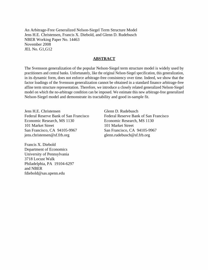
An Arbitrage-Free Generalized Nelson-Siegel Term Structure ModelJens H.E. Christensen, Francis X. Diebold, and Glenn D. RudebuschNBER Working Paper No. 14463November 2008JEL No. G1,G12

ABSTRACT

The Svensson generalization of the popular Nelson-Siegel term structure model is widely used bypractitioners and central banks. Unfortunately, like the original Nelson-Siegel specification, this generalization,in its dynamic form, does not enforce arbitrage-free consistency over time. Indeed, we show that thefactor loadings of the Svensson generalization cannot be obtained in a standard finance arbitrage-freeaffine term structure representation. Therefore, we introduce a closely related generalized Nelson-Siegelmodel on which the no-arbitrage condition can be imposed. We estimate this new arbitrage-free generalizedNelson-Siegel model and demonstrate its tractability and good in-sample fit.

Jens H.E. ChristensenFederal Reserve Bank of San FranciscoEconomic Research, MS 1130101 Market StreetSan Francisco, CA 94105-9967jens.christensen@sf.frb.org

Francis X. DieboldDepartment of EconomicsUniversity of Pennsylvania3718 Locust WalkPhiladelphia, PA 19104-6297and NBERfdiebold@sas.upenn.edu

Glenn D. RudebuschFederal Reserve Bank of San FranciscoEconomic Research, MS 1130101 Market StreetSan Francisco, CA 94105-9967glenn.rudebusch@sf.frb.org

1 Introduction

To investigate yield-curve dynamics, researchers have produced a vast literature with a wide variety

of models. Many of these models assume that at observed bond prices there are no remaining

unexploited opportunities for riskless arbitrage. This theoretical assumption is consistent with the

observation that bonds of various maturities all trade simultaneously in deep and liquid markets.

Rational traders in such markets should enforce a consistency in the yields of various bonds

across different maturities–the yield curve at any point in time–and the expected path of those

yields over time–the dynamic evolution of the yield curve. Indeed, the assumption that there

are no remaining arbitrage opportunities is central to the enormous finance literature devoted to

the empirical analysis of bond pricing. Unfortunately, as noted by Duffee (2002), the associated

arbitrage-free (AF) models can demonstrate disappointing empirical performance, especially with

regard to out-of-sample forecasting. In addition, the estimation of these models is problematic,

in large part because of the existence of numerous model likelihood maxima that have essentially

identical fit to the data but very different implications for economic behavior (Kim and Orphanides,

2005).1

In contrast to the popular finance arbitrage-free models, many other researchers have employed

representations that are empirically appealing but not well grounded in theory. Most notably, the

Nelson-Siegel (1987) curve provides a remarkably good fit to the cross section of yields in many

countries and has become a widely used specification among financial market practitioners and

central banks. Moreover, Diebold and Li (2006) develop a dynamic model based on this curve and

show that it corresponds exactly to a modern factor model, with yields that are affine in three

latent factors, which have a standard interpretation of level, slope, and curvature. Such a dynamic

Nelson-Siegel (DNS) model is easy to estimate and forecasts the yield curve quite well. Despite its

good empirical performance, however, the DNS model does not impose the presumably desirable

theoretical restriction of absence of arbitrage (e.g., Filipovic, 1999, and Diebold, Piazzesi, and

Rudebusch, 2005).

In Christensen, Diebold, and Rudebusch (2007), henceforth CDR, we show how to reconcile the

Nelson-Siegel model with the absence of arbitrage by deriving an affine AF model that maintains

the Nelson-Siegel factor loading structure for the yield curve. This arbitrage-free Nelson-Siegel

(AFNS) model combines the best of both yield-curve modeling traditions. Although it maintains

the theoretical restrictions of the affine AF modeling tradition, the Nelson-Siegel structure helps

identify the latent yield-curve factors, so the AFNS model can be easily and robustly estimated.

Furthermore, our results show that the AFNS model exhibits superior empirical forecasting per-

formance.

In this paper, we consider some important generalizations of the Nelson-Siegel yield curve that

are also widely used in central banks and industry (e.g., De Pooter, 2007).2 Foremost among

these is the Svensson (1995) extension to the Nelson-Siegel curve, which is used at the Federal

1A further failing is that the affine arbitrage-free finance models offer little insight into the economic natureof the underlying forces that drive movements in interest rates. This issue has been addressed by a burgeoningmacro-finance literature, which is described in Rudebusch and Wu (2007, 2008).

2Alternative flexible parameterizations of the yield curve include the use of Legendre polynomials (as in Almeidaand Vicente, 2008) and natural cubic splines (as in Bowsher and Meeks, 2008).

1

Reserve Board (see Gürkaynak, Sack, and Wright, 2007, 2008), the European Central Bank (see

Coroneo, Nyholm, and Vidova-Koleva, 2008), and many other central banks (see Söderlind and

Svensson, 1997, and Bank for International Settlements, 2005). The Svensson extension adds a

second curvature term, which allows for a better fit at long maturities. Following Diebold and

Li (2006), we first introduce a dynamic version of this model, which corresponds to a modern

four-factor term structure model. Unfortunately, we show that it is not possible to obtain an

arbitrage-free “approximation” to this model in the sense of obtaining analytically identical factor

loadings for the four factors. Intuitively, such an approximation requires that each curvature

factor must be paired with a slope factor that has the same mean-reversion rate. This pairing

is simply not possible for the Svensson extension, which has one slope factor and two curvature

factors. Therefore, to obtain an arbitrage-free generalization of the Nelson-Siegel curve, we add a

second slope factor to pair with the second curvature factor. The simple dynamic version of this

model is a generalized version of the DNS model. We also show that the result in CDR can be

extended to obtain an arbitrage-free approximation to that five-factor model, which we refer to as

the arbitrage-free generalized Nelson-Siegel (AFGNS) model.

Finally, we show that this new AFGNS model of the yield curve not only displays theoret-

ical consistency but also retains the important properties of empirical tractability and fit. We

estimate the independent-factor versions of the four-factor and five-factor non-AF models and

the independent-factor version of the five-factor arbitrage-free AFGNS model. We compare the

results to those obtained by CDR for the DNS and AFNS models and find good in-sample fit for

the AFGNS model.

The remainder of the paper is structured as follows. Section 2 briefly describes the DNS model

and its arbitrage-free equivalent as derived in CDR. Section 3 contains the description of the

arbitrage-free generalized Nelson-Siegel model. Section 4 describes the five specific models that

we analyze, while Section 5 describes the data, estimation method, and estimation results. Section

6 concludes the paper, and an appendix contains some additional technical details.

2 Nelson-Siegel term structure models

In this section, we review the DNS and AFNS models that maintain the Nelson-Siegel factor

loading structure.

2.1 The dynamic Nelson-Siegel model

The Nelson-Siegel curve fits the term structure of interest rates at any point in time with the

simple functional form

y(τ) = β0 + β1(1− e−λτ

λτ) + β2(

1− e−λτ

λτ− e−λτ ), (1)

where y(τ) is the zero-coupon yield with τ denoting the time to maturity, and β0, β1, β2, and λ

are model parameters.3

3This is equation (2) in Nelson and Siegel (1987).

2

As many have noted, this representation is able to provide a good fit to the cross section of

yields at a given point in time, and this is a key reason for its popularity with financial market

practitioners. Still, to understand the evolution of the bond market over time, a dynamic rep-

resentation is required. Diebold and Li (2006) supply such a model by replacing the parameters

with time-varying factors

yt(τ) = Lt + St(1− e−λτ

λτ) + Ct(

1− e−λτ

λτ− e−λτ ). (2)

Given their associated Nelson-Siegel factor loadings, Diebold and Li show that Lt, St, and Ct can

be interpreted as level, slope, and curvature factors. Furthermore, once the model is viewed as a

factor model, a dynamic structure can be postulated for the three factors, which yields a dynamic

Nelson-Siegel (DNS) model.

Despite its good empirical performance, however, the DNS model does not impose absence of

arbitrage (e.g., Filipovic, 1999, and Diebold, Piazzesi, and Rudebusch, 2005). This problem was

solved in CDR, where we derived the affine arbitrage-free class of dynamic Nelson-Siegel term

structure models, referred to as the AFNS model in the remainder of this paper.

2.2 The arbitrage-free Nelson-Siegel model

The derivation in CDR of the class of AFNS models starts from the standard continuous-time

affine arbitrage-free term structure model. In this framework, we consider a three-factor model

with a constant volatility matrix, that is, in the terminology of the canonical characterization of

affine term structure models provided by Dai and Singleton (2000), we start with the A0(3) class

of term structure models. Within the A0(3) class, CDR prove the following proposition.

Proposition 2.1. Assume that the instantaneous risk-free rate is defined by

rt = X1t +X2

t .

In addition, assume that the state variables Xt = (X1t ,X

2t ,X

3t ) are described by the following

system of stochastic differential equations (SDEs) under the risk-neutral Q-measure:⎛⎜⎜⎝dX1

t

dX2t

dX3t

⎞⎟⎟⎠ =

⎛⎜⎜⎝0 0 0

0 λ −λ0 0 λ

⎞⎟⎟⎠⎡⎢⎢⎣⎛⎜⎜⎝

θQ1

θQ2

θQ3

⎞⎟⎟⎠−⎛⎜⎜⎝

X1t

X2t

X3t

⎞⎟⎟⎠⎤⎥⎥⎦ dt+Σ

⎛⎜⎜⎝dW 1,Q

t

dW 2,Qt

dW 3,Qt

⎞⎟⎟⎠ , λ > 0.

Then, zero-coupon bond prices are given by

P (t, T )=EQt

£exp

¡−Z T

t

rudu¢¤=exp

¡B1(t, T )X1

t +B2(t, T )X2t +B3(t, T )X3

t + C(t, T )¢,

where B1(t, T ), B2(t, T ), B3(t, T ), and C(t, T ) are the unique solutions to the following system of

3

ordinary differential equations (ODEs):⎛⎜⎜⎝dB1(t,T )

dtdB2(t,T )

dtdB3(t,T )

dt

⎞⎟⎟⎠ =

⎛⎜⎜⎝1

1

0

⎞⎟⎟⎠+⎛⎜⎜⎝0 0 0

0 λ 0

0 −λ λ

⎞⎟⎟⎠⎛⎜⎜⎝

B1(t, T )

B2(t, T )

B3(t, T )

⎞⎟⎟⎠ (3)

anddC(t, T )

dt= −B(t, T )0KQθQ − 1

2

3Xj=1

¡Σ0B(t, T )B(t, T )0Σ

¢j,j, (4)

with boundary conditions B1(T, T ) = B2(T, T ) = B3(T, T ) = C(T, T ) = 0. The unique solution

for this system of ODEs is:

B1(t, T ) = −(T − t),

B2(t, T ) = −1− e−λ(T−t)

λ,

B3(t, T ) = (T − t)e−λ(T−t) − 1− e−λ(T−t)

λ,

and

C(t, T ) = (KQθQ)2

Z T

t

B2(s, T )ds+ (KQθQ)3

Z T

t

B3(s, T )ds

+1

2

3Xj=1

Z T

t

¡Σ0B(s, T )B(s, T )0Σ

¢j,jds.

Finally, zero-coupon bond yields are given by

y(t, T ) = X1t +

1− e−λ(T−t)

λ(T − t)X2t +

h1− e−λ(T−t)

λ(T − t)− e−λ(T−t)

iX3t −

C(t, T )

T − t.

For proof see CDR.

This proposition defines the class of AFNS models. In this class of models, the factor loadings

exactly match the Nelson-Siegel ones, but there is an unavoidable additional term in the yield

function, −C(t,T )T−t , which depends only on the maturity of the bond. This “yield-adjustment”

term is a crucial difference between the AFNS and DNS models and has the following form:4

−C(t, T )T − t

= −12

1

T − t

3Xj=1

Z T

t

¡Σ0B(s, T )B(s, T )0Σ

¢j,jds.

4As explained in CDR, this form of the yield-adjustment term is obtained by fixing the mean parameters of thestate variables under the Q-measure at zero, i.e., θQ = 0, which implies no loss of generality.

4

Given a general volatility matrix

Σ =

⎛⎜⎜⎝σ11 σ12 σ13

σ21 σ22 σ23

σ31 σ32 σ33

⎞⎟⎟⎠ ,

the yield-adjustment term can be derived in analytical form as

C(t, T )

T − t=

1

2

1

T − t

Z T

t

3Xj=1

¡Σ0B(s, T )B(s, T )0Σ

¢j,jds

= A(T − t)2

6+B

h 12λ2− 1

λ31− e−λ(T−t)

T − t+

1

4λ31− e−2λ(T−t)

T − t

i+ C

h 12λ2

+1

λ2e−λ(T−t) − 1

4λ(T − t)e−2λ(T−t) − 3

4λ2e−2λ(T−t)

− 2λ31− e−λ(T−t)

T − t+

5

8λ31− e−2λ(T−t)

T − t

i+ D

h 12λ(T − t) +

1

λ2e−λ(T−t) − 1

λ31− e−λ(T−t)

T − t

i+ E

h 3λ2

e−λ(T−t) +1

2λ(T − t) +

1

λ(T − t)e−λ(T−t) − 3

λ31− e−λ(T−t)

T − t

i+ F

h 1λ2+1

λ2e−λ(T−t) − 1

2λ2e−2λ(T−t) − 3

λ31− e−λ(T−t)

T − t

+3

4λ31− e−2λ(T−t)

T − t

i,

where

• A = σ211 + σ212 + σ213,

• B = σ221 + σ222 + σ223,

• C = σ231 + σ232 + σ233,

• D = σ11σ21 + σ12σ22 + σ13σ23,

• E = σ11σ31 + σ12σ32 + σ13σ33,

• F = σ21σ31 + σ22σ32 + σ23σ33.

This result has two implications. First, the fact that zero-coupon bond yields in the AFNS class

of models are given by an analytical formula greatly facilitates empirical implementation of these

models. Second, the nine underlying volatility parameters are not identified. Indeed, only the six

terms A, B, C, D, E, and F can be identified; thus, the maximally flexible AFNS specification

that can be identified has a triangular volatility matrix given by5

Σ =

⎛⎜⎜⎝σ11 0 0

σ21 σ22 0

σ31 σ32 σ33

⎞⎟⎟⎠ .

5The choice of upper or lower triangular is irrelevant for the fit of the model.

5

3 Extensions of the Nelson-Siegel model

The main in-sample problem with the regular Nelson-Siegel yield curve is that, for reasonable

choices of λ (which are empirically in the range from 0.5 to 1 for U.S. Treasury yield data),

the factor loading for the slope and the curvature factor decay rapidly to zero as a function of

maturity. Thus, only the level factor is available to fit yields with maturities of ten years or

longer. In empirical estimation, this limitation shows up as a lack of fit of the long-term yields,

as described in CDR.

To address this problem in fitting the cross section of yields, Svensson (1995) introduced an

extended version of the Nelson-Siegel yield curve with an additional curvature factor,

y(τ) = β1 + β2

³1− e−λ1τ

λ1τ

´+ β3

³1− e−λ1τ

λ1τ− e−λ1τ

´+ β4

³1− e−λ2τ

λ2τ− e−λ2τ

´.

Just as Diebold and Li (2006) replaced the three β coefficients with dynamic factors in the regular

Nelson-Siegel model, we can replace the four β coefficients in the Svensson model with dynamic

processes (Lt, St, C1t , C2t ) interpreted as a level, a slope, and two curvature factors, respectively.

Thus, the dynamic factor model representation of the Svensson yield curve, which we label the

DNSS model, is given by

yt(τ) = Lt + St

³1− e−λ1τ

λ1τ

´+ C1t

³1− e−λ1τ

λ1τ− e−λ1τ

´+ C2t

³1− e−λ2τ

λ2τ− e−λ2τ

´,

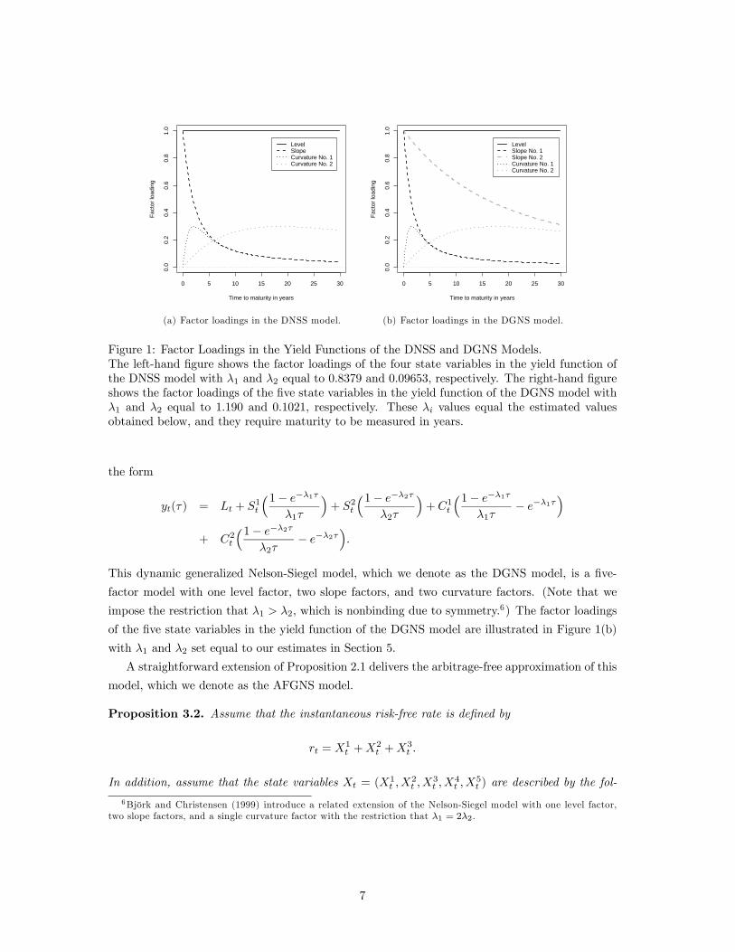
along with the processes describing factor dynamics. The factor loadings of the four state variables

in the yield function of the DNSS model are illustrated in Figure 1(a) with λ1 and λ2 set equal to

our estimates described in Section 5.

The critique raised by Filipovic (1999) against the dynamic version of the Nelson-Siegel model

also applies to the dynamic version of the Svensson model introduced in this paper. Thus, this

model is not consistent with the concept of absence of arbitrage. Ideally, we would like to repeat

the work in CDR and derive an arbitrage-free approximation to the DNSS model. However, from

the mechanics of Proposition 2.1 for the arbitrage-free approximation of the regular Nelson-Siegel

model, it is clear that we can only obtain the Nelson-Siegel factor loading structure for the slope

and curvature factors under two specific conditions. First, each pair of slope and curvature factors

must have identical own mean-reversion rates. Second, the impact of deviations in the curvature

factor from its mean on the slope factor must be scaled with a factor equal to that own mean-

reversion rate (λ). Thus, it is impossible in an arbitrage-free model to generate the factor loading

structure of two curvature factors with only one slope factor. Consequently, it is impossible to

create an arbitrage-free version of the Svensson extension to the Nelson-Siegel model that has

factor loadings analytically identical to the ones in the DNSS model.

However, this discussion suggests that we can create a generalized AF Nelson-Siegel model by

including a fifth factor in the form of a second slope factor. The yield function of this model takes

6

0 5 10 15 20 25 30

0.0

0.2

0.4

0.6

0.8

1.0

Time to maturity in years

Fac

tor

load

ing

Level Slope Curvature No. 1 Curvature No. 2

(a) Factor loadings in the DNSS model.

0 5 10 15 20 25 30

0.0

0.2

0.4

0.6

0.8

1.0

Time to maturity in years

Fac

tor

load

ing

Level Slope No. 1 Slope No. 2 Curvature No. 1 Curvature No. 2

(b) Factor loadings in the DGNS model.

Figure 1: Factor Loadings in the Yield Functions of the DNSS and DGNS Models.The left-hand figure shows the factor loadings of the four state variables in the yield function ofthe DNSS model with λ1 and λ2 equal to 0.8379 and 0.09653, respectively. The right-hand figureshows the factor loadings of the five state variables in the yield function of the DGNS model withλ1 and λ2 equal to 1.190 and 0.1021, respectively. These λi values equal the estimated valuesobtained below, and they require maturity to be measured in years.

the form

yt(τ) = Lt + S1t

³1− e−λ1τ

λ1τ

´+ S2t

³1− e−λ2τ

λ2τ

´+ C1t

³1− e−λ1τ

λ1τ− e−λ1τ

´+ C2t

³1− e−λ2τ

λ2τ− e−λ2τ

´.

This dynamic generalized Nelson-Siegel model, which we denote as the DGNS model, is a five-

factor model with one level factor, two slope factors, and two curvature factors. (Note that we

impose the restriction that λ1 > λ2, which is nonbinding due to symmetry.6) The factor loadings

of the five state variables in the yield function of the DGNS model are illustrated in Figure 1(b)

with λ1 and λ2 set equal to our estimates in Section 5.

A straightforward extension of Proposition 2.1 delivers the arbitrage-free approximation of this

model, which we denote as the AFGNS model.

Proposition 3.2. Assume that the instantaneous risk-free rate is defined by

rt = X1t +X2

t +X3t .

In addition, assume that the state variables Xt = (X1t ,X

2t ,X

3t ,X

4t ,X

5t ) are described by the fol-

6Björk and Christensen (1999) introduce a related extension of the Nelson-Siegel model with one level factor,two slope factors, and a single curvature factor with the restriction that λ1 = 2λ2.

7

lowing system of SDEs under the risk-neutral Q-measure:⎛⎜⎜⎜⎜⎜⎜⎜⎝

dX1t

dX2t

dX3t

dX4t

dX5t

⎞⎟⎟⎟⎟⎟⎟⎟⎠=

⎛⎜⎜⎜⎜⎜⎜⎜⎝

0 0 0 0 0

0 λ1 0 −λ1 0

0 0 λ2 0 −λ20 0 0 λ1 0

0 0 0 0 λ2

⎞⎟⎟⎟⎟⎟⎟⎟⎠

⎡⎢⎢⎢⎢⎢⎢⎢⎣

⎛⎜⎜⎜⎜⎜⎜⎜⎝

θQ1

θQ2

θQ3

θQ4

θQ5

⎞⎟⎟⎟⎟⎟⎟⎟⎠−

⎛⎜⎜⎜⎜⎜⎜⎜⎝

X1t

X2t

X3t

X4t

X5t

⎞⎟⎟⎟⎟⎟⎟⎟⎠

⎤⎥⎥⎥⎥⎥⎥⎥⎦dt+Σ

⎛⎜⎜⎜⎜⎜⎜⎜⎝

dW 1,Qt

dW 2,Qt

dW 3,Qt

dW 4,Qt

dW 5,Qt

⎞⎟⎟⎟⎟⎟⎟⎟⎠where λ1 > λ2 > 0.

Then, zero-coupon bond prices are given by

P (t, T ) = EQt

£exp

¡−Z T

t

rudu¢¤

= exp¡B1(t, T )X1

t +B2(t, T )X2t +B3(t, T )X3

t

+ B4(t, T )X4t +B5(t, T )X5

t + C(t, T )¢,

where B1(t, T ), B2(t, T ), B3(t, T ), B4(t, T ), B5(t, T ), and C(t, T ) are the unique solutions to the

following system of ODEs:⎛⎜⎜⎜⎜⎜⎜⎜⎝

dB1(t,T )dt

dB2(t,T )dt

dB3(t,T )dt

dB4(t,T )dt

dB5(t,T )dt

⎞⎟⎟⎟⎟⎟⎟⎟⎠=

⎛⎜⎜⎜⎜⎜⎜⎜⎝

1

1

1

0

0

⎞⎟⎟⎟⎟⎟⎟⎟⎠+

⎛⎜⎜⎜⎜⎜⎜⎜⎝

0 0 0 0 0

0 λ1 0 0 0

0 0 λ2 0 0

0 −λ1 0 λ1 0

0 0 −λ2 0 λ2

⎞⎟⎟⎟⎟⎟⎟⎟⎠

⎛⎜⎜⎜⎜⎜⎜⎜⎝

B1(t, T )

B2(t, T )

B3(t, T )

B4(t, T )

B5(t, T )

⎞⎟⎟⎟⎟⎟⎟⎟⎠(5)

anddC(t, T )

dt= −B(t, T )0KQθQ − 1

2

5Xj=1

¡Σ0B(t, T )B(t, T )0Σ

¢j,j, (6)

with boundary conditions B1(T, T ) = B2(T, T ) = B3(T, T ) = B4(T, T ) = B5(T, T ) = C(T, T ) =

0. The unique solution for this system of ODEs is:

B1(t, T ) = −(T − t),

B2(t, T ) = −1− e−λ1(T−t)

λ1,

B3(t, T ) = −1− e−λ2(T−t)

λ2,

B4(t, T ) = (T − t)e−λ1(T−t) − 1− e−λ1(T−t)

λ1,

B5(t, T ) = (T − t)e−λ2(T−t) − 1− e−λ2(T−t)

λ2,

8

and

C(t, T ) = (KQθQ)2

Z T

t

B2(s, T )ds+ (KQθQ)3

Z T

t

B3(s, T )ds+ (KQθQ)4

Z T

t

B4(s, T )ds

+ (KQθQ)5

Z T

t

B5(s, T )ds+1

2

5Xj=1

Z T

t

¡Σ0B(s, T )B(s, T )0Σ

¢j,jds.

Finally, zero-coupon bond yields are given by

y(t, T ) = X1t +

1− e−λ1(T−t)

λ1(T − t)X2t +

1− e−λ2(T−t)

λ2(T − t)X3t +

h1− e−λ1(T−t)

λ1(T − t)− e−λ1(T−t)

iX4t

+h1− e−λ2(T−t)

λ2(T − t)− e−λ2(T−t)

iX5t −

C(t, T )

T − t.

The proof is a straightforward extension of CDR.

Similar to the AFNS class of models, the yield-adjustment term will have the following form:7

−C(t, T )T − t

= −12

1

T − t

5Xj=1

Z T

t

¡Σ0B(s, T )B(s, T )0Σ

¢j,jds.

Following arguments similar to the ones provided for the AFNS class of models in the previ-

ous section, the maximally flexible specification of the volatility matrix that can be identified in

estimation is given by a triangular matrix

Σ =

⎛⎜⎜⎜⎜⎜⎜⎜⎝

σ11 0 0 0 0

σ21 σ22 0 0 0

σ31 σ32 σ33 0 0

σ41 σ42 σ43 σ44 0

σ51 σ52 σ53 σ54 σ55

⎞⎟⎟⎟⎟⎟⎟⎟⎠.

4 Five specific Nelson-Siegel models

In general, all the models considered in this paper are silent about the P -dynamics, and an infinite

number of possible specifications could be used to match the data. However, for continuity with

the existing literature, our econometric analysis focuses on independent-factor versions of the five

different models we have described. These models include the DNS and AFNS models from CDR

and the generalized DNSS, DGNS, and AFGNS models introduced in Section 3.

In the independent-factor DNS model, all three state variables are assumed to be independent

first-order autoregressions, as in Diebold and Li (2006). Using their notation, the state equation

7The analytical formula for the yield-adjustment term in the AFGNS model is provided in Appendix A. As wasthe case for Proposition 2.1, Proposition 3.2 is also silent about the P -dynamics of the state variables, so to identifythe model, we follow CDR and fix the mean under the Q-measure at zero, i.e., θQ = 0.

9

is given by ⎛⎜⎜⎝Lt − μL

St − μS

Ct − μC

⎞⎟⎟⎠ =

⎛⎜⎜⎝a11 0 0

0 a22 0

0 0 a33

⎞⎟⎟⎠⎛⎜⎜⎝

Lt−1 − μL

St−1 − μS

Ct−1 − μC

⎞⎟⎟⎠+⎛⎜⎜⎝

ηt(L)

ηt(S)

ηt(C)

⎞⎟⎟⎠ ,

where the error terms ηt(L), ηt(S), and ηt(C) have a conditional covariance matrix given by

Q =

⎛⎜⎜⎝q211 0 0

0 q222 0

0 0 q233

⎞⎟⎟⎠ .

In this model, the measurement equation takes the form⎛⎜⎜⎜⎜⎜⎝yt(τ1)

yt(τ2)...

yt(τN )

⎞⎟⎟⎟⎟⎟⎠ =

⎛⎜⎜⎜⎜⎜⎝1 1−e−λτ1

λτ11−e−λτ1

λτ1− e−λτ1

1 1−e−λτ2λτ2

1−e−λτ2λτ2

− e−λτ2

......

...

1 1−e−λτNλτN

1−e−λτNλτN

− e−λτN

⎞⎟⎟⎟⎟⎟⎠⎛⎜⎜⎝

Lt

St

Ct

⎞⎟⎟⎠+⎛⎜⎜⎜⎜⎜⎝

εt(τ1)

εt(τ2)...

εt(τN )

⎞⎟⎟⎟⎟⎟⎠ ,

where the measurement errors εt(τi) are assumed to be independently and identically distributed

(i.i.d.) white noise.

The corresponding AFNS model is formulated in continuous time and the relationship between

the real-world dynamics under the P -measure and the risk-neutral dynamics under the Q-measure

is given by the measure change

dWQt = dWP

t + Γtdt,

where Γt represents the risk premium specification. To preserve affine dynamics under the P -

measure, we limit our focus to essentially affine risk premium specifications (see Duffee, 2002).

Thus, Γt will take the form

Γt =

⎛⎜⎜⎝γ01

γ02

γ03

⎞⎟⎟⎠+⎛⎜⎜⎝

γ111 γ112 γ113

γ121 γ122 γ123

γ131 γ132 γ133

⎞⎟⎟⎠⎛⎜⎜⎝

X1t

X2t

X3t

⎞⎟⎟⎠ .

With this specification, the SDE for the state variables under the P -measure,

dXt = KP [θP −Xt]dt+ΣdWPt , (7)

remains affine. Due to the flexible specification of Γt, we are free to choose any mean vector θP

and mean-reversion matrix KP under the P -measure and still preserve the required Q-dynamic

structure described in Proposition 2.1. Therefore, we focus on the independent-factor AFNS model,

which corresponds to the specific DNS model from earlier in this section and assumes all three

factors are independent under the P -measure

10

⎛⎜⎜⎝dX1

t

dX2t

dX3t

⎞⎟⎟⎠ =

⎛⎜⎜⎝κP11 0 0

0 κP22 0

0 0 κP33

⎞⎟⎟⎠⎡⎢⎢⎣⎛⎜⎜⎝

θP1

θP2

θP3

⎞⎟⎟⎠−⎛⎜⎜⎝

X1t

X2t

X3t

⎞⎟⎟⎠⎤⎥⎥⎦ dt+

⎛⎜⎜⎝σ1 0 0

0 σ2 0

0 0 σ3

⎞⎟⎟⎠⎛⎜⎜⎝dW 1,P

t

dW 2,Pt

dW 3,Pt

⎞⎟⎟⎠ .

In this case, the measurement equation takes the form⎛⎜⎜⎜⎜⎜⎝yt(τ1)

yt(τ2)...

yt(τN )

⎞⎟⎟⎟⎟⎟⎠ =

⎛⎜⎜⎜⎜⎜⎝1 1−e−λτ1

λτ11−e−λτ1

λτ1− e−λτ1

1 1−e−λτ2λτ2

1−e−λτ2λτ2

− e−λτ2

......

...

1 1−e−λτNλτN

1−e−λτNλτN

− e−λτN

⎞⎟⎟⎟⎟⎟⎠⎛⎜⎜⎝X1t

X2t

X3t

⎞⎟⎟⎠−⎛⎜⎜⎜⎜⎜⎝

C(τ1)τ1

C(τ2)τ2

...C(τN)τN

⎞⎟⎟⎟⎟⎟⎠+⎛⎜⎜⎜⎜⎜⎝εt(τ1)

εt(τ2)...

εt(τN )

⎞⎟⎟⎟⎟⎟⎠ ,

where, again, the measurement errors εt(τi) are assumed to be i.i.d. white noise.

We now turn to the three generalized Nelson-Siegel models. In the independent-factor DNSS

model, all four state variables are assumed to be independent first-order autoregressions, as in

Diebold and Li (2006). Using their notation, the state equation is given by⎛⎜⎜⎜⎜⎝Lt − μL

St − μS

C1t − μC1

C2t − μC2

⎞⎟⎟⎟⎟⎠ =

⎛⎜⎜⎜⎜⎝a11 0 0 0

0 a22 0 0

0 0 a33 0

0 0 0 a44

⎞⎟⎟⎟⎟⎠⎛⎜⎜⎜⎜⎝

Lt−1 − μL

St−1 − μS

C1t−1 − μC1

C2t−1 − μC2

⎞⎟⎟⎟⎟⎠+⎛⎜⎜⎜⎜⎝

ηt(L)

ηt(S)

ηt(C1)

ηt(C2)

⎞⎟⎟⎟⎟⎠ ,

where the error terms ηt(L), ηt(S), ηt(C1), and ηt(C2) have a conditional covariance matrix given

by

Q =

⎛⎜⎜⎜⎜⎝q211 0 0 0

0 q222 0 0

0 0 q233 0

0 0 0 q244

⎞⎟⎟⎟⎟⎠ .

In the DNSS model, the measurement equation takes the form⎛⎜⎜⎜⎜⎜⎝yt(τ1)

yt(τ2)...

yt(τN )

⎞⎟⎟⎟⎟⎟⎠=⎛⎜⎜⎜⎜⎜⎝1 1−e−λ1τ1

λ1τ11−e−λ1τ1

λ1τ1− e−λ1τ1 1−e−λ2τ1

λ2τ1− e−λ2τ1

1 1−e−λ1τ2λ1τ2

1−e−λ1τ2λ1τ2

− e−λ1τ2 1−e−λ2τ2λ2τ2

− e−λ2τ2

......

......

1 1−e−λ1τNλ1τN

1−e−λ1τNλ1τN

− e−λ1τN 1−e−λ2τNλ2τN

− e−λ2τN

⎞⎟⎟⎟⎟⎟⎠⎛⎜⎜⎜⎜⎝Lt

St

C1t

C2t

⎞⎟⎟⎟⎟⎠+⎛⎜⎜⎜⎜⎜⎝εt(τ1)

εt(τ2)...

εt(τN )

⎞⎟⎟⎟⎟⎟⎠,

where the measurement errors εt(τi) are assumed to be i.i.d. white noise.

In the independent-factor DGNS model, all five state variables are assumed to be independent

11

first-order autoregressions, and the state equation is given by⎛⎜⎜⎜⎜⎜⎜⎜⎝

Lt − μL

S1t − μS1

S2t − μS2

C1t − μC1

C2t − μC2

⎞⎟⎟⎟⎟⎟⎟⎟⎠=

⎛⎜⎜⎜⎜⎜⎜⎜⎝

a11 0 0 0 0

0 a22 0 0 0

0 0 a33 0 0

0 0 0 a44 0

0 0 0 0 a55

⎞⎟⎟⎟⎟⎟⎟⎟⎠

⎛⎜⎜⎜⎜⎜⎜⎜⎝

Lt−1 − μL

S1t−1 − μS1

S2t−1 − μS2

C1t−1 − μC1

C2t−1 − μC2

⎞⎟⎟⎟⎟⎟⎟⎟⎠+

⎛⎜⎜⎜⎜⎜⎜⎜⎝

ηt(L)

ηt(S1)

ηt(S2)

ηt(C1)

ηt(C2)

⎞⎟⎟⎟⎟⎟⎟⎟⎠,

where the error terms ηt(L), ηt(S1), ηt(S2), ηt(C1), and ηt(C2) have a conditional covariance

matrix given by

Q =

⎛⎜⎜⎜⎜⎜⎜⎜⎝

q211 0 0 0 0

0 q222 0 0 0

0 0 q233 0 0

0 0 0 q244 0

0 0 0 0 q255

⎞⎟⎟⎟⎟⎟⎟⎟⎠.

In the DGNS model, the measurement equation takes the form

⎛⎜⎜⎜⎜⎜⎝yt(τ1)

yt(τ2)...

yt(τN )

⎞⎟⎟⎟⎟⎟⎠ =

⎛⎜⎜⎜⎜⎜⎝1 1−e−λ1τ1

λ1τ11−e−λ2τ1

λ2τ11−e−λ1τ1

λ1τ1− e−λ1τ1 1−e−λ2τ1

λ2τ1− e−λ2τ1

1 1−e−λ1τ2λ1τ2

1−e−λ2τ2λ2τ2

1−e−λ1τ2λ1τ2

− e−λ1τ2 1−e−λ2τ2λ2τ2

− e−λ2τ2

......

......

...

1 1−e−λ1τNλ1τN

1−e−λ2τNλ2τN

1−e−λ1τNλ1τN

− e−λ1τN 1−e−λ2τNλ2τN

− e−λ2τN

⎞⎟⎟⎟⎟⎟⎠

⎛⎜⎜⎜⎜⎜⎜⎜⎝

Lt

S1t

S2t

C1t

C2t

⎞⎟⎟⎟⎟⎟⎟⎟⎠

+

⎛⎜⎜⎜⎜⎜⎝εt(τ1)

εt(τ2)...

εt(τN )

⎞⎟⎟⎟⎟⎟⎠ ,

where the measurement errors εt(τi) are assumed to be i.i.d. white noise.

Finally, as for the AFNS model, the AFGNS model is formulated in continuous time and the

relationship between the real-world dynamics under the P -measure and the risk-neutral dynamics

under the Q-measure is given by the measure change

dWQt = dWP

t + Γtdt,

where Γt represents the risk premium specification. Again, to preserve affine dynamics under the

P -measure, we limit our focus to essentially affine risk premium specifications (see Duffee, 2002).

12

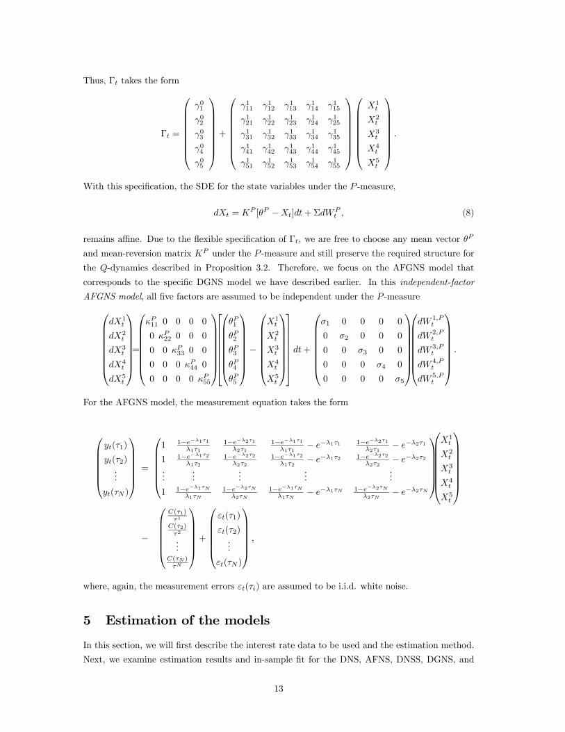
Thus, Γt takes the form

Γt =

⎛⎜⎜⎜⎜⎜⎜⎜⎝

γ01

γ02

γ03

γ04

γ05

⎞⎟⎟⎟⎟⎟⎟⎟⎠+

⎛⎜⎜⎜⎜⎜⎜⎜⎝

γ111 γ112 γ113 γ114 γ115

γ121 γ122 γ123 γ124 γ125

γ131 γ132 γ133 γ134 γ135

γ141 γ142 γ143 γ144 γ145

γ151 γ152 γ153 γ154 γ155

⎞⎟⎟⎟⎟⎟⎟⎟⎠

⎛⎜⎜⎜⎜⎜⎜⎜⎝

X1t

X2t

X3t

X4t

X5t

⎞⎟⎟⎟⎟⎟⎟⎟⎠.

With this specification, the SDE for the state variables under the P -measure,

dXt = KP [θP −Xt]dt+ΣdWPt , (8)

remains affine. Due to the flexible specification of Γt, we are free to choose any mean vector θP

and mean-reversion matrix KP under the P -measure and still preserve the required structure for

the Q-dynamics described in Proposition 3.2. Therefore, we focus on the AFGNS model that

corresponds to the specific DGNS model we have described earlier. In this independent-factor

AFGNS model, all five factors are assumed to be independent under the P -measure⎛⎜⎜⎜⎜⎜⎜⎜⎝

dX1t

dX2t

dX3t

dX4t

dX5t

⎞⎟⎟⎟⎟⎟⎟⎟⎠=

⎛⎜⎜⎜⎜⎜⎜⎜⎝

κP11 0 0 0 0

0 κP22 0 0 0

0 0 κP33 0 0

0 0 0 κP44 0

0 0 0 0 κP55

⎞⎟⎟⎟⎟⎟⎟⎟⎠

⎡⎢⎢⎢⎢⎢⎢⎢⎣

⎛⎜⎜⎜⎜⎜⎜⎜⎝

θP1

θP2

θP3

θP4

θP5

⎞⎟⎟⎟⎟⎟⎟⎟⎠−

⎛⎜⎜⎜⎜⎜⎜⎜⎝

X1t

X2t

X3t

X4t

X5t

⎞⎟⎟⎟⎟⎟⎟⎟⎠

⎤⎥⎥⎥⎥⎥⎥⎥⎦dt+

⎛⎜⎜⎜⎜⎜⎜⎜⎝

σ1 0 0 0 0

0 σ2 0 0 0

0 0 σ3 0 0

0 0 0 σ4 0

0 0 0 0 σ5

⎞⎟⎟⎟⎟⎟⎟⎟⎠

⎛⎜⎜⎜⎜⎜⎜⎜⎝

dW 1,Pt

dW 2,Pt

dW 3,Pt

dW 4,Pt

dW 5,Pt

⎞⎟⎟⎟⎟⎟⎟⎟⎠.

For the AFGNS model, the measurement equation takes the form

⎛⎜⎜⎜⎜⎜⎝yt(τ1)

yt(τ2)...

yt(τN )

⎞⎟⎟⎟⎟⎟⎠ =

⎛⎜⎜⎜⎜⎜⎝1 1−e−λ1τ1

λ1τ11−e−λ2τ1

λ2τ11−e−λ1τ1

λ1τ1− e−λ1τ1 1−e−λ2τ1

λ2τ1− e−λ2τ1

1 1−e−λ1τ2λ1τ2

1−e−λ2τ2λ2τ2

1−e−λ1τ2λ1τ2

− e−λ1τ2 1−e−λ2τ2λ2τ2

− e−λ2τ2

......

......

...

1 1−e−λ1τNλ1τN

1−e−λ2τNλ2τN

1−e−λ1τNλ1τN

− e−λ1τN 1−e−λ2τNλ2τN

− e−λ2τN

⎞⎟⎟⎟⎟⎟⎠

⎛⎜⎜⎜⎜⎜⎜⎜⎝

X1t

X2t

X3t

X4t

X5t

⎞⎟⎟⎟⎟⎟⎟⎟⎠

−

⎛⎜⎜⎜⎜⎜⎝C(τ1)τ1

C(τ2)τ2

...C(τN)τN

⎞⎟⎟⎟⎟⎟⎠+⎛⎜⎜⎜⎜⎜⎝εt(τ1)

εt(τ2)...

εt(τN )

⎞⎟⎟⎟⎟⎟⎠ ,

where, again, the measurement errors εt(τi) are assumed to be i.i.d. white noise.

5 Estimation of the models

In this section, we will first describe the interest rate data to be used and the estimation method.

Next, we examine estimation results and in-sample fit for the DNS, AFNS, DNSS, DGNS, and

13

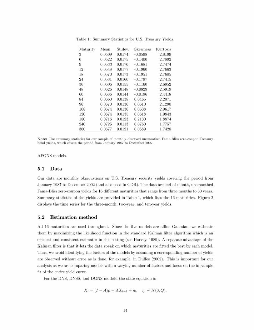
Table 1: Summary Statistics for U.S. Treasury Yields.

Maturity Mean St.dev. Skewness Kurtosis3 0.0509 0.0174 -0.0598 2.81996 0.0522 0.0175 -0.1400 2.78929 0.0533 0.0176 -0.1681 2.747412 0.0548 0.0177 -0.1960 2.766318 0.0570 0.0173 -0.1951 2.760524 0.0581 0.0166 -0.1797 2.741536 0.0606 0.0155 -0.1160 2.695248 0.0626 0.0148 -0.0829 2.591960 0.0636 0.0144 -0.0196 2.441884 0.0660 0.0138 0.0465 2.207196 0.0670 0.0136 0.0610 2.1290108 0.0674 0.0136 0.0638 2.0617120 0.0674 0.0135 0.0618 1.9843180 0.0716 0.0123 0.2130 1.8874240 0.0725 0.0113 0.0760 1.7757360 0.0677 0.0121 0.0589 1.7428

Note: The summary statistics for our sample of monthly observed unsmoothed Fama-Bliss zero-coupon Treasurybond yields, which covers the period from January 1987 to December 2002.

AFGNS models.

5.1 Data

Our data are monthly observations on U.S. Treasury security yields covering the period from

January 1987 to December 2002 (and also used in CDR). The data are end-of-month, unsmoothed

Fama-Bliss zero-coupon yields for 16 different maturities that range from three months to 30 years.

Summary statistics of the yields are provided in Table 1, which lists the 16 maturities. Figure 2

displays the time series for the three-month, two-year, and ten-year yields.

5.2 Estimation method

All 16 maturities are used throughout. Since the five models are affine Gaussian, we estimate

them by maximizing the likelihood function in the standard Kalman filter algorithm which is an

efficient and consistent estimator in this setting (see Harvey, 1989). A separate advantage of the

Kalman filter is that it lets the data speak on which maturities are fitted the best by each model.

Thus, we avoid identifying the factors of the models by assuming a corresponding number of yields

are observed without error as is done, for example, in Duffee (2002). This is important for our

analysis as we are comparing models with a varying number of factors and focus on the in-sample

fit of the entire yield curve.

For the DNS, DNSS, and DGNS models, the state equation is

Xt = (I −A)μ+AXt−1 + ηt, ηt ∼ N(0, Q),

14

1990 1995 2000

0.00

0.02

0.04

0.06

0.08

0.10

Time

Yie

ld

10−year yield 2−year yield 3−month yield

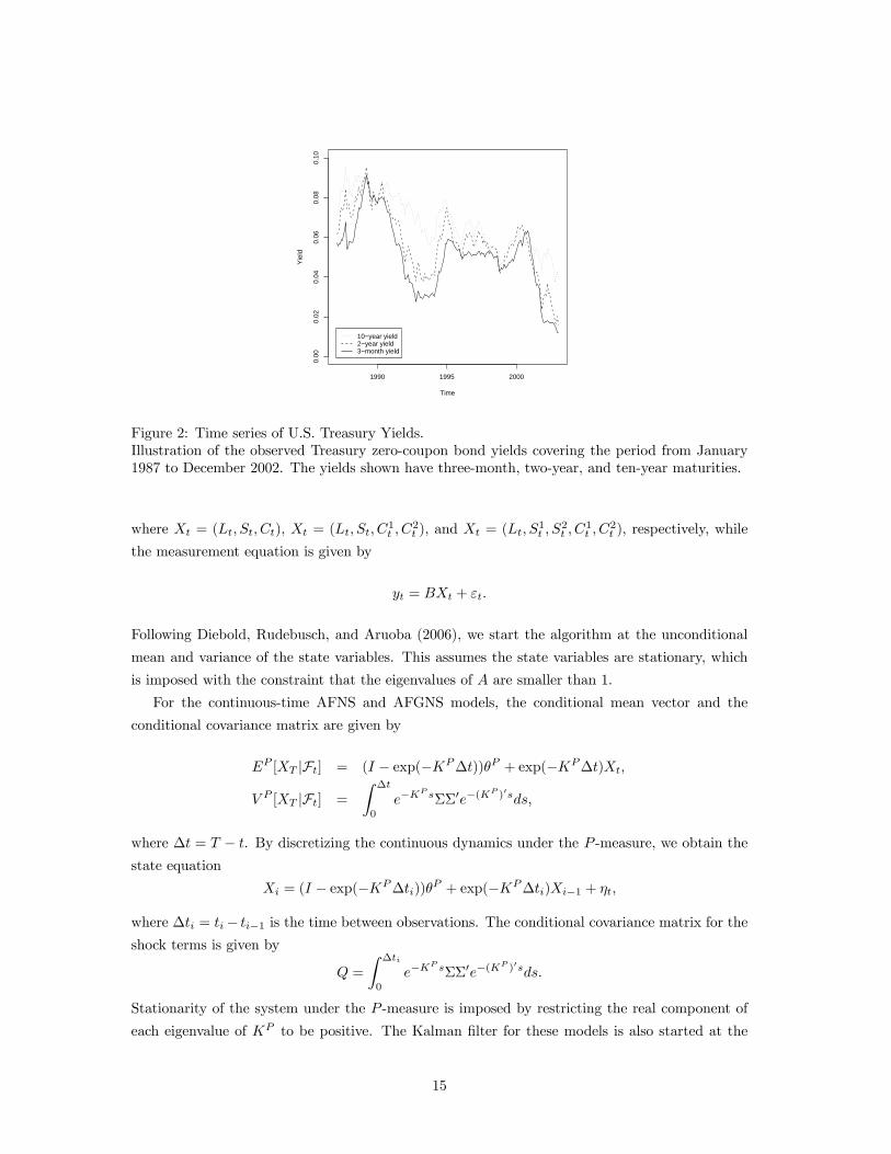
Figure 2: Time series of U.S. Treasury Yields.Illustration of the observed Treasury zero-coupon bond yields covering the period from January1987 to December 2002. The yields shown have three-month, two-year, and ten-year maturities.

where Xt = (Lt, St, Ct), Xt = (Lt, St, C1t , C

2t ), and Xt = (Lt, S

1t , S

2t , C

1t , C

2t ), respectively, while

the measurement equation is given by

yt = BXt + εt.

Following Diebold, Rudebusch, and Aruoba (2006), we start the algorithm at the unconditional

mean and variance of the state variables. This assumes the state variables are stationary, which

is imposed with the constraint that the eigenvalues of A are smaller than 1.

For the continuous-time AFNS and AFGNS models, the conditional mean vector and the

conditional covariance matrix are given by

EP [XT |Ft] = (I − exp(−KP∆t))θP + exp(−KP∆t)Xt,

V P [XT |Ft] =

Z ∆t0

e−KP sΣΣ0e−(K

P )0sds,

where ∆t = T − t. By discretizing the continuous dynamics under the P -measure, we obtain the

state equation

Xi = (I − exp(−KP∆ti))θP + exp(−KP∆ti)Xi−1 + ηt,

where ∆ti = ti− ti−1 is the time between observations. The conditional covariance matrix for the

shock terms is given by

Q =

Z ∆ti0

e−KP sΣΣ0e−(K

P )0sds.

Stationarity of the system under the P -measure is imposed by restricting the real component of

each eigenvalue of KP to be positive. The Kalman filter for these models is also started at the

15

unconditional mean and covariance8

bX0 = θP and bΣ0 = Z ∞0

e−KP sΣΣ0e−(K

P )0sds.

Finally, the AFNS and AFGNS measurement equation is given by

yt = A+BXt + εt.

For all five models, the error structure isÃηt

εt

!∼ N

"Ã0

0

!,

ÃQ 0

0 H

!#,

where H is a diagonal matrix for the measurement errors of the 16 maturities used in estimation

H =

⎛⎜⎜⎝σ2(τ1) . . . 0...

. . ....

0 . . . σ2(τ16)

⎞⎟⎟⎠ .

The linear least-squares optimality of the Kalman filter requires that the transition and measure-

ment errors be orthogonal to the initial state, i.e.,

E[f0η0t] = 0, E[f0ε

0t] = 0.

Finally, parameter standard deviations are calculated as

Σ( bψ) = 1

T

h 1T

TXt=1

∂ log lt( bψ)∂ψ

∂ log lt( bψ)∂ψ

0i−1,

where bψ denotes the estimated model parameter set.5.3 DNSS model estimation results

Table 2 presents the estimated mean-reversion matrix A and the estimated vector of mean para-

meters μ, along with the estimated parameters of the conditional covariance matrix Q obtained for

the DNSS model. The results reveal that the slope factor is the most persistent factor. Also, the

relatively large standard deviations of the estimated mean parameters suggest some difficulty in

pinning down their value under the P -measure, which is likely related to the fairly high persistence

of the state variables (e.g., Kim and Orphanides, 2005). The λ1 parameter is estimated at 0.838,

which implies a factor loading for the first curvature factor that peaks near the two-year maturity.

The estimated value of λ2 is 0.097, so the factor loading of the second curvature factor reaches

its maximum near the 19-year maturity. (These are illustrated in Figure 1(a).) Clearly, the two

curvature factors take on very different roles in the fit of the model.

8 In the estimation, ∞0 e−K

P sΣΣ0e−(KP )0sds is approximated by 10

0 e−KP sΣΣ0e−(K

P )0sds.

16

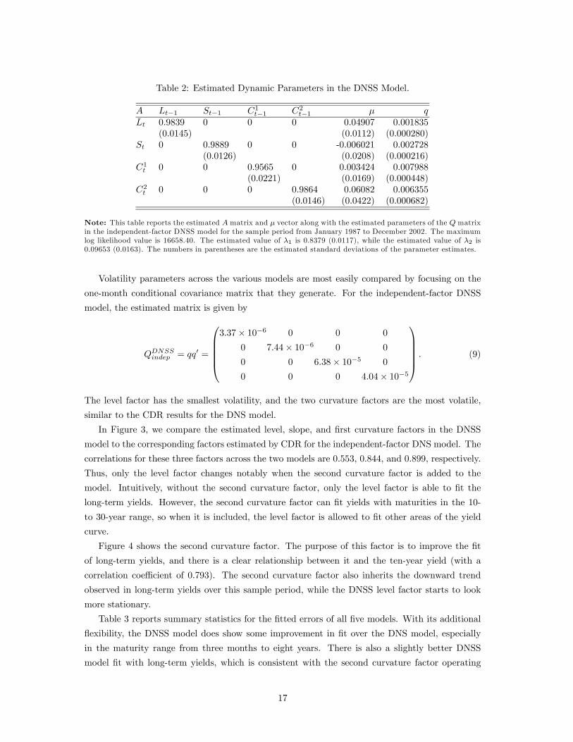
Table 2: Estimated Dynamic Parameters in the DNSS Model.

A Lt−1 St−1 C1t−1 C2t−1 μ qLt 0.9839 0 0 0 0.04907 0.001835

(0.0145) (0.0112) (0.000280)St 0 0.9889 0 0 -0.006021 0.002728

(0.0126) (0.0208) (0.000216)C1t 0 0 0.9565 0 0.003424 0.007988

(0.0221) (0.0169) (0.000448)C2t 0 0 0 0.9864 0.06082 0.006355

(0.0146) (0.0422) (0.000682)

Note: This table reports the estimated A matrix and μ vector along with the estimated parameters of the Q matrixin the independent-factor DNSS model for the sample period from January 1987 to December 2002. The maximumlog likelihood value is 16658.40. The estimated value of λ1 is 0.8379 (0.0117), while the estimated value of λ2 is0.09653 (0.0163). The numbers in parentheses are the estimated standard deviations of the parameter estimates.

Volatility parameters across the various models are most easily compared by focusing on the

one-month conditional covariance matrix that they generate. For the independent-factor DNSS

model, the estimated matrix is given by

QDNSSindep = qq0 =

⎛⎜⎜⎜⎜⎝3.37× 10−6 0 0 0

0 7.44× 10−6 0 0

0 0 6.38× 10−5 0

0 0 0 4.04× 10−5

⎞⎟⎟⎟⎟⎠ . (9)

The level factor has the smallest volatility, and the two curvature factors are the most volatile,

similar to the CDR results for the DNS model.

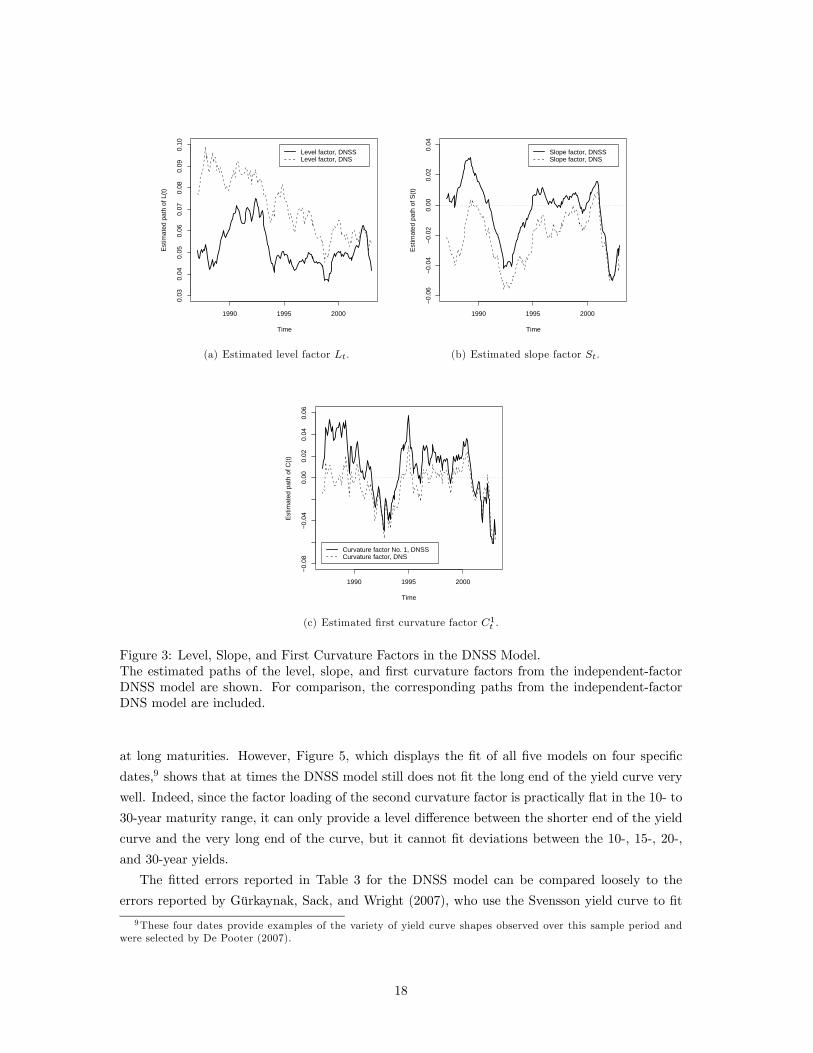
In Figure 3, we compare the estimated level, slope, and first curvature factors in the DNSS

model to the corresponding factors estimated by CDR for the independent-factor DNS model. The

correlations for these three factors across the two models are 0.553, 0.844, and 0.899, respectively.

Thus, only the level factor changes notably when the second curvature factor is added to the

model. Intuitively, without the second curvature factor, only the level factor is able to fit the

long-term yields. However, the second curvature factor can fit yields with maturities in the 10-

to 30-year range, so when it is included, the level factor is allowed to fit other areas of the yield

curve.

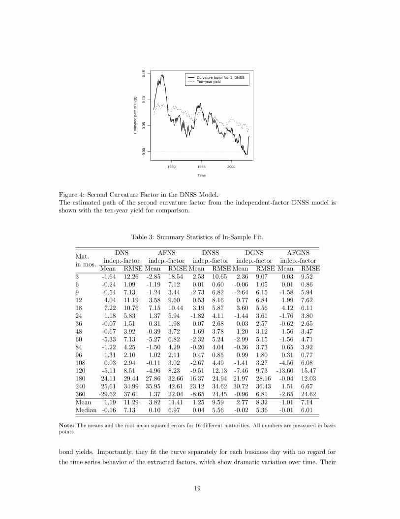
Figure 4 shows the second curvature factor. The purpose of this factor is to improve the fit

of long-term yields, and there is a clear relationship between it and the ten-year yield (with a

correlation coefficient of 0.793). The second curvature factor also inherits the downward trend

observed in long-term yields over this sample period, while the DNSS level factor starts to look

more stationary.

Table 3 reports summary statistics for the fitted errors of all five models. With its additional

flexibility, the DNSS model does show some improvement in fit over the DNS model, especially

in the maturity range from three months to eight years. There is also a slightly better DNSS

model fit with long-term yields, which is consistent with the second curvature factor operating

17

1990 1995 2000

0.03

0.04

0.05

0.06

0.07

0.08

0.09

0.10

Time

Est

imat

ed p

ath

of L

(t)

Level factor, DNSS Level factor, DNS

(a) Estimated level factor Lt.

1990 1995 2000

−0.

06−

0.04

−0.

020.

000.

020.

04

Time

Est

imat

ed p

ath

of S

(t)

Slope factor, DNSS Slope factor, DNS

(b) Estimated slope factor St.

1990 1995 2000

−0.

08−

0.04

0.00

0.02

0.04

0.06

Time

Est

imat

ed p

ath

of C

(t)

Curvature factor No. 1, DNSS Curvature factor, DNS

(c) Estimated first curvature factor C1t .

Figure 3: Level, Slope, and First Curvature Factors in the DNSS Model.The estimated paths of the level, slope, and first curvature factors from the independent-factorDNSS model are shown. For comparison, the corresponding paths from the independent-factorDNS model are included.

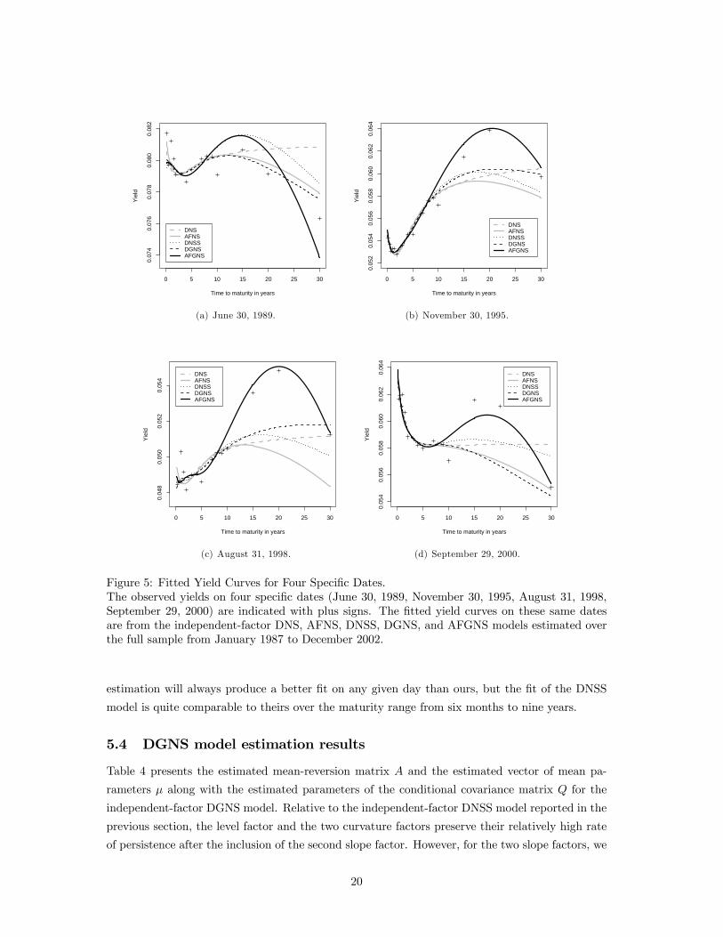
at long maturities. However, Figure 5, which displays the fit of all five models on four specific

dates,9 shows that at times the DNSS model still does not fit the long end of the yield curve very

well. Indeed, since the factor loading of the second curvature factor is practically flat in the 10- to

30-year maturity range, it can only provide a level difference between the shorter end of the yield

curve and the very long end of the curve, but it cannot fit deviations between the 10-, 15-, 20-,

and 30-year yields.

The fitted errors reported in Table 3 for the DNSS model can be compared loosely to the

errors reported by Gürkaynak, Sack, and Wright (2007), who use the Svensson yield curve to fit

9These four dates provide examples of the variety of yield curve shapes observed over this sample period andwere selected by De Pooter (2007).

18

1990 1995 2000

0.00

0.05

0.10

0.15

Time

Est

imat

ed p

ath

of C

2(t)

Curvature factor No. 2, DNSS Ten−year yield

Figure 4: Second Curvature Factor in the DNSS Model.The estimated path of the second curvature factor from the independent-factor DNSS model isshown with the ten-year yield for comparison.

Table 3: Summary Statistics of In-Sample Fit.

DNS AFNS DNSS DGNS AFGNSMat.indep.-factor indep.-factor indep.-factor indep.-factor indep.-factorin mos.Mean RMSE Mean RMSEMean RMSEMean RMSE Mean RMSE

3 -1.64 12.26 -2.85 18.54 2.53 10.65 2.36 9.07 0.03 9.526 -0.24 1.09 -1.19 7.12 0.01 0.60 -0.06 1.05 0.01 0.869 -0.54 7.13 -1.24 3.44 -2.73 6.82 -2.64 6.15 -1.58 5.9412 4.04 11.19 3.58 9.60 0.53 8.16 0.77 6.84 1.99 7.6218 7.22 10.76 7.15 10.44 3.19 5.87 3.60 5.56 4.12 6.1124 1.18 5.83 1.37 5.94 -1.82 4.11 -1.44 3.61 -1.76 3.8036 -0.07 1.51 0.31 1.98 0.07 2.68 0.03 2.57 -0.62 2.6548 -0.67 3.92 -0.39 3.72 1.69 3.78 1.20 3.12 1.56 3.4760 -5.33 7.13 -5.27 6.82 -2.32 5.24 -2.99 5.15 -1.56 4.7184 -1.22 4.25 -1.50 4.29 -0.26 4.04 -0.36 3.73 0.65 3.9296 1.31 2.10 1.02 2.11 0.47 0.85 0.99 1.80 0.31 0.77108 0.03 2.94 -0.11 3.02 -2.67 4.49 -1.41 3.27 -4.56 6.08120 -5.11 8.51 -4.96 8.23 -9.51 12.13 -7.46 9.73 -13.60 15.47180 24.11 29.44 27.86 32.66 16.37 24.94 21.97 28.16 -0.04 12.03240 25.61 34.99 35.95 42.61 23.12 34.62 30.72 36.43 1.51 6.67360 -29.62 37.61 1.37 22.04 -8.65 24.45 -0.96 6.81 -2.65 24.62Mean 1.19 11.29 3.82 11.41 1.25 9.59 2.77 8.32 -1.01 7.14Median -0.16 7.13 0.10 6.97 0.04 5.56 -0.02 5.36 -0.01 6.01

Note: The means and the root mean squared errors for 16 different maturities. All numbers are measured in basispoints.

bond yields. Importantly, they fit the curve separately for each business day with no regard for

the time series behavior of the extracted factors, which show dramatic variation over time. Their

19

0 5 10 15 20 25 30

0.07

40.

076

0.07

80.

080

0.08

2

Time to maturity in years

Yie

ld

DNS AFNS DNSS DGNS AFGNS

(a) June 30, 1989.

0 5 10 15 20 25 30

0.05

20.

054

0.05

60.

058

0.06

00.

062

0.06

4

Time to maturity in years

Yie

ld

DNS AFNS DNSS DGNS AFGNS

(b) November 30, 1995.

0 5 10 15 20 25 30

0.04

80.

050

0.05

20.

054

Time to maturity in years

Yie

ld

DNS AFNS DNSS DGNS AFGNS

(c) August 31, 1998.

0 5 10 15 20 25 30

0.05

40.

056

0.05

80.

060

0.06

20.

064

Time to maturity in years

Yie

ldDNS AFNS DNSS DGNS AFGNS

(d) September 29, 2000.

Figure 5: Fitted Yield Curves for Four Specific Dates.The observed yields on four specific dates (June 30, 1989, November 30, 1995, August 31, 1998,September 29, 2000) are indicated with plus signs. The fitted yield curves on these same datesare from the independent-factor DNS, AFNS, DNSS, DGNS, and AFGNS models estimated overthe full sample from January 1987 to December 2002.

estimation will always produce a better fit on any given day than ours, but the fit of the DNSS

model is quite comparable to theirs over the maturity range from six months to nine years.

5.4 DGNS model estimation results

Table 4 presents the estimated mean-reversion matrix A and the estimated vector of mean pa-

rameters μ along with the estimated parameters of the conditional covariance matrix Q for the

independent-factor DGNS model. Relative to the independent-factor DNSS model reported in the

previous section, the level factor and the two curvature factors preserve their relatively high rate

of persistence after the inclusion of the second slope factor. However, for the two slope factors, we

20

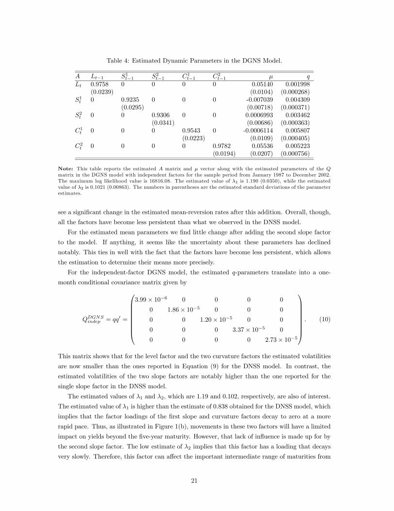
Table 4: Estimated Dynamic Parameters in the DGNS Model.

A Lt−1 S1t−1 S2t−1 C1t−1 C2t−1 μ qLt 0.9758 0 0 0 0 0.05140 0.001998

(0.0239) (0.0104) (0.000268)S1t 0 0.9235 0 0 0 -0.007039 0.004309

(0.0295) (0.00718) (0.000371)S2t 0 0 0.9306 0 0 0.0006993 0.003462

(0.0341) (0.00686) (0.000363)C1t 0 0 0 0.9543 0 -0.0006114 0.005807

(0.0223) (0.0109) (0.000405)C2t 0 0 0 0 0.9782 0.05536 0.005223

(0.0194) (0.0207) (0.000756)

Note: This table reports the estimated A matrix and μ vector along with the estimated parameters of the Qmatrix in the DGNS model with independent factors for the sample period from January 1987 to December 2002.The maximum log likelihood value is 16816.08. The estimated value of λ1 is 1.190 (0.0350), while the estimatedvalue of λ2 is 0.1021 (0.00863). The numbers in parentheses are the estimated standard deviations of the parameterestimates.

see a significant change in the estimated mean-reversion rates after this addition. Overall, though,

all the factors have become less persistent than what we observed in the DNSS model.

For the estimated mean parameters we find little change after adding the second slope factor

to the model. If anything, it seems like the uncertainty about these parameters has declined

notably. This ties in well with the fact that the factors have become less persistent, which allows

the estimation to determine their means more precisely.

For the independent-factor DGNS model, the estimated q-parameters translate into a one-

month conditional covariance matrix given by

QDGNSindep = qq0 =

⎛⎜⎜⎜⎜⎜⎜⎜⎝

3.99× 10−6 0 0 0 0

0 1.86× 10−5 0 0 0

0 0 1.20× 10−5 0 0

0 0 0 3.37× 10−5 0

0 0 0 0 2.73× 10−5

⎞⎟⎟⎟⎟⎟⎟⎟⎠. (10)

This matrix shows that for the level factor and the two curvature factors the estimated volatilities

are now smaller than the ones reported in Equation (9) for the DNSS model. In contrast, the

estimated volatilities of the two slope factors are notably higher than the one reported for the

single slope factor in the DNSS model.

The estimated values of λ1 and λ2, which are 1.19 and 0.102, respectively, are also of interest.

The estimated value of λ1 is higher than the estimate of 0.838 obtained for the DNSS model, which

implies that the factor loadings of the first slope and curvature factors decay to zero at a more

rapid pace. Thus, as illustrated in Figure 1(b), movements in these two factors will have a limited

impact on yields beyond the five-year maturity. However, that lack of influence is made up for by

the second slope factor. The low estimate of λ2 implies that this factor has a loading that decays

very slowly. Therefore, this factor can affect the important intermediate range of maturities from

21

1990 1995 2000

0.03

0.04

0.05

0.06

0.07

0.08

0.09

0.10

Time

Est

imat

ed p

ath

of L

(t)

Level factor, DGNS Level factor, DNSS Level factor, DNS

(a) The estimated level factor Lt.

1990 1995 2000

−0.

06−

0.04

−0.

020.

000.

020.

04

Time

Est

imat

ed p

ath

of S

(t)

Slope factor No. 1, DGNS Slope factor, DNSS Slope factor, DNS

(b) The estimated first slope factor S1t .

1990 1995 2000

−0.

050.

000.

05

Time

Est

imat

ed p

ath

of C

1(t)

Curvature factor No. 1, DGNS Curvature factor No. 1, DNSS Curvature factor, DNS

(c) The estimated first curvature factor C1t .

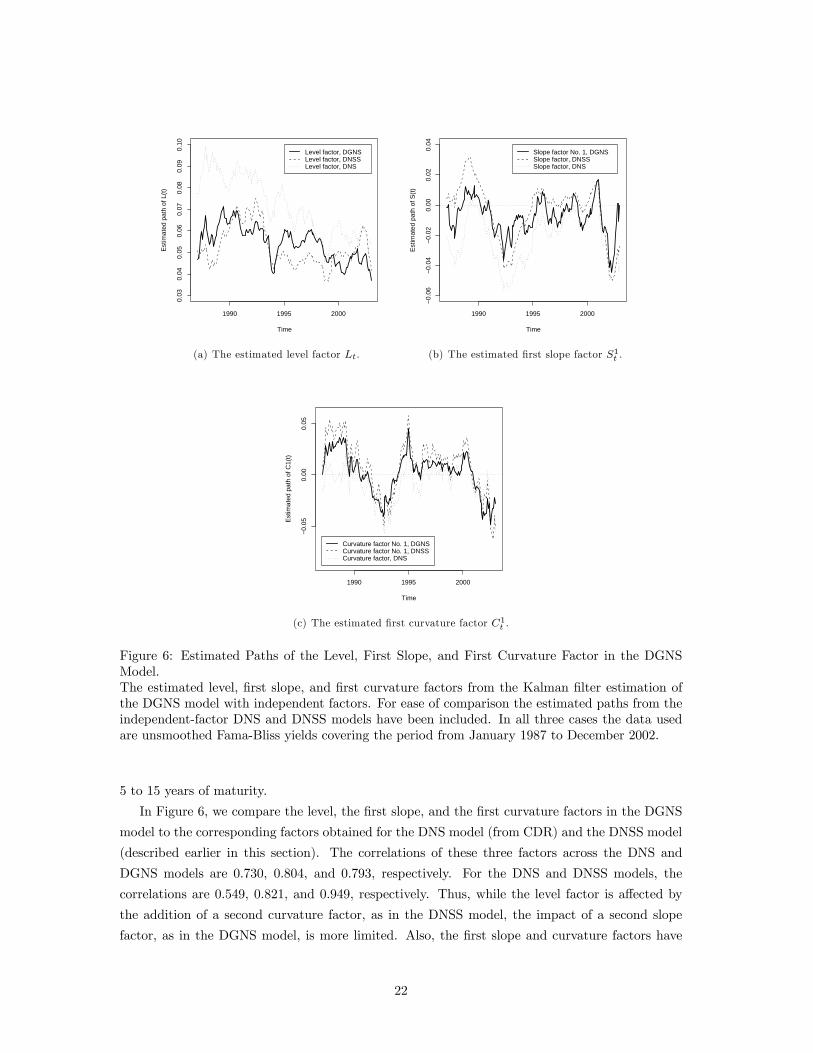
Figure 6: Estimated Paths of the Level, First Slope, and First Curvature Factor in the DGNSModel.The estimated level, first slope, and first curvature factors from the Kalman filter estimation ofthe DGNS model with independent factors. For ease of comparison the estimated paths from theindependent-factor DNS and DNSS models have been included. In all three cases the data usedare unsmoothed Fama-Bliss yields covering the period from January 1987 to December 2002.

5 to 15 years of maturity.

In Figure 6, we compare the level, the first slope, and the first curvature factors in the DGNS

model to the corresponding factors obtained for the DNS model (from CDR) and the DNSS model

(described earlier in this section). The correlations of these three factors across the DNS and

DGNS models are 0.730, 0.804, and 0.793, respectively. For the DNS and DNSS models, the

correlations are 0.549, 0.821, and 0.949, respectively. Thus, while the level factor is affected by

the addition of a second curvature factor, as in the DNSS model, the impact of a second slope

factor, as in the DGNS model, is more limited. Also, the first slope and curvature factors have

22

1990 1995 2000

−0.

02−

0.01

0.00

0.01

0.02

Time

Est

imat

ed p

ath

of S

2(t)

(a) The estimated second slope factor S2t .

1990 1995 2000

0.00

0.05

0.10

0.15

Time

Est

imat

ed p

ath

of C

2(t)

Curvature factor No. 2, DGNS Curvature factor No. 2, DNSS Ten−year yield

(b) The estimated second curvature factor C2t .

Figure 7: Second Slope and Second Curvature Factors in the DGNS Model.The estimated paths of the second slope and curvature factors of the independent-factor DGNSmodel. The estimated path of the second curvature factor from the independent-factor DNSSmodel has been included for comparison.

very similar sample paths across all three models. Given the fairly large estimated values of λ1 in

all three models, the factor loadings of these two factors decay towards zero relatively rapidly as

a function of maturity, so their roles in fitting the shorter end of the yield curve are well defined.

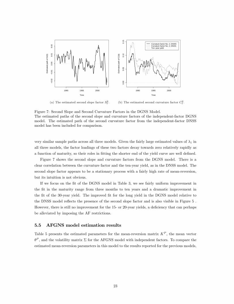
Figure 7 shows the second slope and curvature factors from the DGNS model. There is a

clear correlation between the curvature factor and the ten-year yield, as in the DNSS model. The

second slope factor appears to be a stationary process with a fairly high rate of mean-reversion,

but its intuition is not obvious.

If we focus on the fit of the DGNS model in Table 3, we see fairly uniform improvement in

the fit in the maturity range from three months to ten years and a dramatic improvement in

the fit of the 30-year yield. The improved fit for the long yield in the DGNS model relative to

the DNSS model reflects the presence of the second slope factor and is also visible in Figure 5 .

However, there is still no improvement for the 15- or 20-year yields, a deficiency that can perhaps

be alleviated by imposing the AF restrictions.

5.5 AFGNS model estimation results

Table 5 presents the estimated parameters for the mean-reversion matrix KP , the mean vector

θP , and the volatility matrix Σ for the AFGNS model with independent factors. To compare the

estimated mean-reversion parameters in this model to the results reported for the previous models,

23

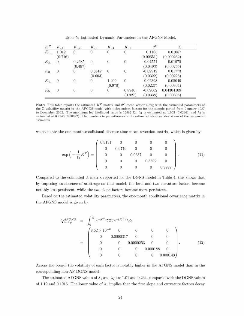
Table 5: Estimated Dynamic Parameters in the AFGNS Model.

KP K·,1 K·,2 K·,3 K·,4 K·,5 θP ΣK1,· 1.012 0 0 0 0 0.1165 0.01057

(0.716) (0.00651) (0.000262)K2,· 0 0.2685 0 0 0 -0.04551 0.01975

(0.497) (0.0493) (0.00255)K3,· 0 0 0.3812 0 0 -0.02912 0.01773

(0.603) (0.0322) (0.00225)K4,· 0 0 0 1.409 0 -0.02398 0.05049

(0.970) (0.0227) (0.00304)K5,· 0 0 0 0 0.8940 -0.09662 0.04304109

(0.927) (0.0338) (0.00305)

Note: This table reports the estimated KP matrix and θP mean vector along with the estimated parameters ofthe Σ volatility matrix in the AFGNS model with independent factors for the sample period from January 1987to December 2002. The maximum log likelihood value is 16982.52. λ1 is estimated at 1.005 (0.0246), and λ2 isestimated at 0.2343 (0.00922). The numbers in parentheses are the estimated standard deviations of the parameterestimates.

we calculate the one-month conditional discrete-time mean-reversion matrix, which is given by

exp³− 1

12KP

´=

⎛⎜⎜⎜⎜⎜⎜⎜⎝

0.9191 0 0 0 0

0 0.9779 0 0 0

0 0 0.9687 0 0

0 0 0 0.8892 0

0 0 0 0 0.9282

⎞⎟⎟⎟⎟⎟⎟⎟⎠. (11)

Compared to the estimated A matrix reported for the DGNS model in Table 4, this shows that

by imposing an absence of arbitrage on that model, the level and two curvature factors become

notably less persistent, while the two slope factors become more persistent.

Based on the estimated volatility parameters, the one-month conditional covariance matrix in

the AFGNS model is given by

QAFGNSindep =

Z 112

0

e−KP sΣΣ0e−(K

P )0sds

=

⎛⎜⎜⎜⎜⎜⎜⎜⎝

8.52× 10−6 0 0 0 0

0 0.0000317 0 0 0

0 0 0.0000253 0 0

0 0 0 0.000188 0

0 0 0 0 0.000143

⎞⎟⎟⎟⎟⎟⎟⎟⎠. (12)

Across the board, the volatility of each factor is notably higher in the AFGNS model than in the

corresponding non-AF DGNS model.

The estimated AFGNS values of λ1 and λ2 are 1.01 and 0.234, compared with the DGNS values

of 1.19 and 0.1016. The lower value of λ1 implies that the first slope and curvature factors decay

24

1990 1995 2000

0.03

0.04

0.05

0.06

0.07

0.08

0.09

0.10

Time

Est

imat

ed p

ath

of L

(t)

Level factor − 0.05, AFGNS Level factor, DGNS Level factor, DNSS Level factor, DNS

(a) The estimated level factor Lt.

1990 1995 2000

−0.

10−

0.05

0.00

0.05

Time

Est

imat

ed p

ath

of S

1(t)

Slope factor No. 1, AFGNS Slope factor No. 1, DGNS Slope factor, DNSS Slope factor, DNS

(b) The estimated first slope factor S1t .

1990 1995 2000

−0.

10−

0.05

0.00

0.05

Time

Est

imat

ed p

ath

of C

1(t)

Curvature factor No. 1, AFGNS Curvature factor No. 1, DGNS Curvature factor No. 1, DNSS Curvature factor, DNS

(c) The estimated first curvature factor C1t .

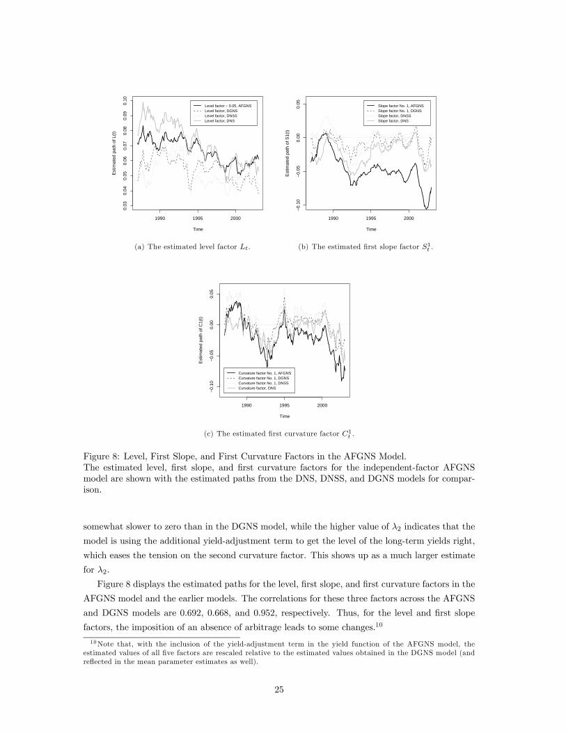
Figure 8: Level, First Slope, and First Curvature Factors in the AFGNS Model.The estimated level, first slope, and first curvature factors for the independent-factor AFGNSmodel are shown with the estimated paths from the DNS, DNSS, and DGNS models for compar-ison.

somewhat slower to zero than in the DGNS model, while the higher value of λ2 indicates that the

model is using the additional yield-adjustment term to get the level of the long-term yields right,

which eases the tension on the second curvature factor. This shows up as a much larger estimate

for λ2.

Figure 8 displays the estimated paths for the level, first slope, and first curvature factors in the

AFGNS model and the earlier models. The correlations for these three factors across the AFGNS

and DGNS models are 0.692, 0.668, and 0.952, respectively. Thus, for the level and first slope

factors, the imposition of an absence of arbitrage leads to some changes.10

10Note that, with the inclusion of the yield-adjustment term in the yield function of the AFGNS model, theestimated values of all five factors are rescaled relative to the estimated values obtained in the DGNS model (andreflected in the mean parameter estimates as well).

25

1990 1995 2000

−0.

06−

0.04

−0.

020.

000.

02

Time

Est

imat

ed p

ath

of S

2(t)

Slope factor No. 2, AFGNS Slope factor No. 2, DGNS

(a) The estimated second slope factor S2t .

1990 1995 2000

0.00

0.05

0.10

0.15

Time

Est

imat

ed p

ath

of C

2(t)

Curvature factor No. 2 + 0.15, AFGNS Curvature factor No. 2, DGNS Curvature factor No. 2, DNSS Ten−year yield

(b) The estimated second curvature factor C2t .

Figure 9: Second Slope and Second Curvature Factors in the AFGNS Model.The estimated second slope and curvature factors for the independent-factor AFGNS model areshown with corresponding estimated paths from the DNSS and DGNS models for comparison.

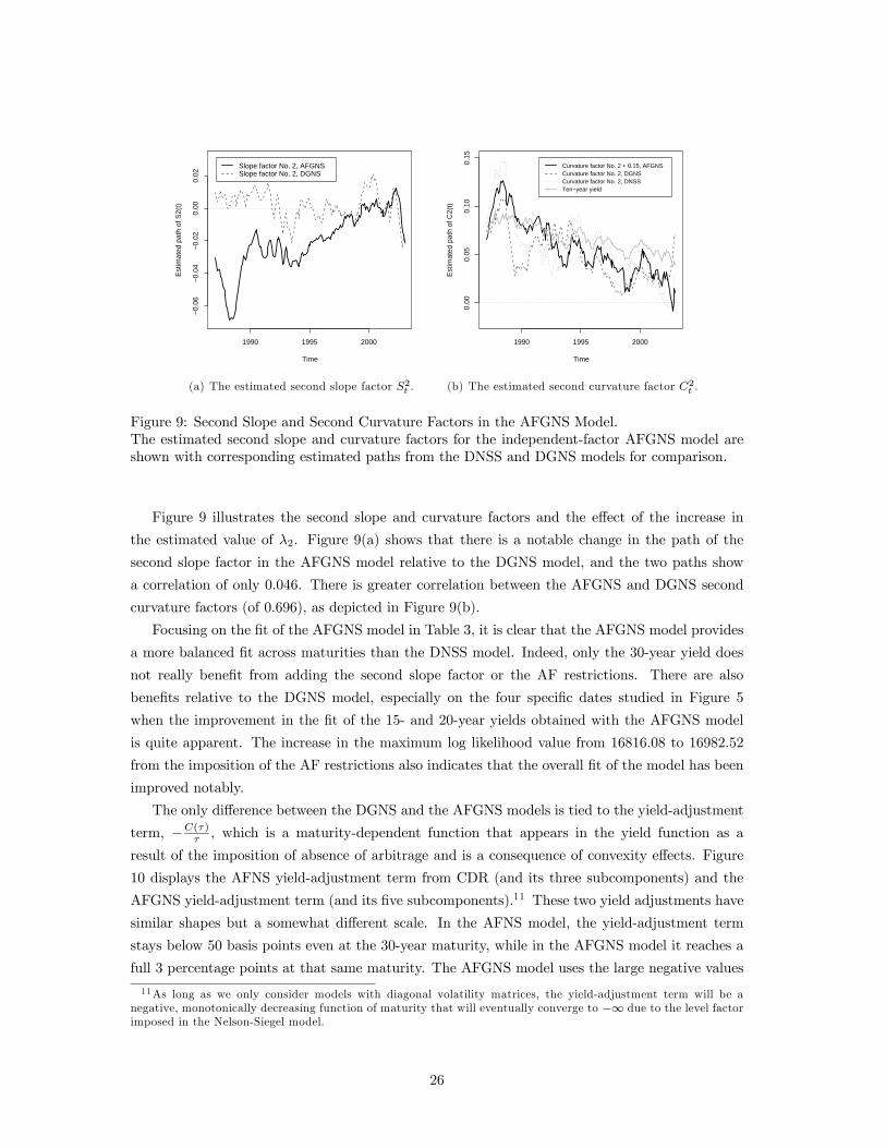
Figure 9 illustrates the second slope and curvature factors and the effect of the increase in

the estimated value of λ2. Figure 9(a) shows that there is a notable change in the path of the

second slope factor in the AFGNS model relative to the DGNS model, and the two paths show

a correlation of only 0.046. There is greater correlation between the AFGNS and DGNS second

curvature factors (of 0.696), as depicted in Figure 9(b).

Focusing on the fit of the AFGNS model in Table 3, it is clear that the AFGNS model provides

a more balanced fit across maturities than the DNSS model. Indeed, only the 30-year yield does

not really benefit from adding the second slope factor or the AF restrictions. There are also

benefits relative to the DGNS model, especially on the four specific dates studied in Figure 5

when the improvement in the fit of the 15- and 20-year yields obtained with the AFGNS model

is quite apparent. The increase in the maximum log likelihood value from 16816.08 to 16982.52

from the imposition of the AF restrictions also indicates that the overall fit of the model has been

improved notably.

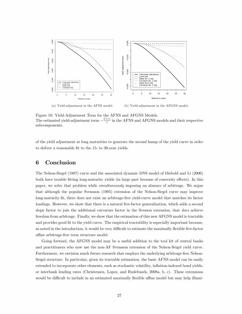
The only difference between the DGNS and the AFGNS models is tied to the yield-adjustment

term, −C(τ)τ , which is a maturity-dependent function that appears in the yield function as a

result of the imposition of absence of arbitrage and is a consequence of convexity effects. Figure

10 displays the AFNS yield-adjustment term from CDR (and its three subcomponents) and the

AFGNS yield-adjustment term (and its five subcomponents).11 These two yield adjustments have

similar shapes but a somewhat different scale. In the AFNS model, the yield-adjustment term

stays below 50 basis points even at the 30-year maturity, while in the AFGNS model it reaches a

full 3 percentage points at that same maturity. The AFGNS model uses the large negative values

11As long as we only consider models with diagonal volatility matrices, the yield-adjustment term will be anegative, monotonically decreasing function of maturity that will eventually converge to −∞ due to the level factorimposed in the Nelson-Siegel model.

26

0 5 10 15 20 25 30

−0.

005

−0.

004

−0.

003

−0.

002

−0.

001

0.00

0

Maturity in years

Yie

ld−

adju

stm

ent t

erm

Total yield−adjustment Level only Slope only Curvature only

(a) Yield-adjustment in the AFNS model.

0 5 10 15 20 25 30

−0.

030

−0.

020

−0.

010

0.00

0

Maturity in years

Yie

ld−

adju

stm

ent t

erm

Total yield−adjustment Level only Slope No. 1 only Curvature No. 1 only Slope No.2 only Curvature No. 2 only

(b) Yield-adjustment in the AFGNS model.

Figure 10: Yield-Adjustment Term for the AFNS and AFGNS Models.The estimated yield-adjustment term −C(τ)

τ in the AFNS and AFGNS models and their respectivesubcomponents.

of the yield adjustment at long maturities to generate the second hump of the yield curve in order

to deliver a reasonable fit to the 15- to 30-year yields.

6 Conclusion

The Nelson-Siegel (1987) curve and the associated dynamic DNS model of Diebold and Li (2006)

both have trouble fitting long-maturity yields (in large part because of convexity effects). In this

paper, we solve that problem while simultaneously imposing an absence of arbitrage. We argue

that although the popular Svensson (1995) extension of the Nelson-Siegel curve may improve

long-maturity fit, there does not exist an arbitrage-free yield-curve model that matches its factor

loadings. However, we show that there is a natural five-factor generalization, which adds a second

slope factor to join the additional curvature factor in the Svesson extension, that does achieve

freedom from arbitrage. Finally, we show that the estimation of this new AFGNSmodel is tractable

and provides good fit to the yield curve. The empirical tractability is especially important because,

as noted in the introduction, it would be very difficult to estimate the maximally flexible five-factor

affine arbitrage-free term structure model.

Going forward, the AFGNS model may be a useful addition to the tool kit of central banks

and practitioners who now use the non-AF Svensson extension of the Nelson-Seigel yield curve.

Furthermore, we envision much future research that employs the underlying arbitrage-free Nelson-

Seigel structure. In particular, given its tractable estimation, the basic AFNS model can be easily

extended to incorporate other elements, such as stochastic volatility, inflation-indexed bond yields,

or interbank lending rates (Christensen, Lopez, and Rudebusch, 2008a, b, c). These extensions

would be difficult to include in an estimated maximally flexible affine model but may help illumi-

27

nate various important issues.

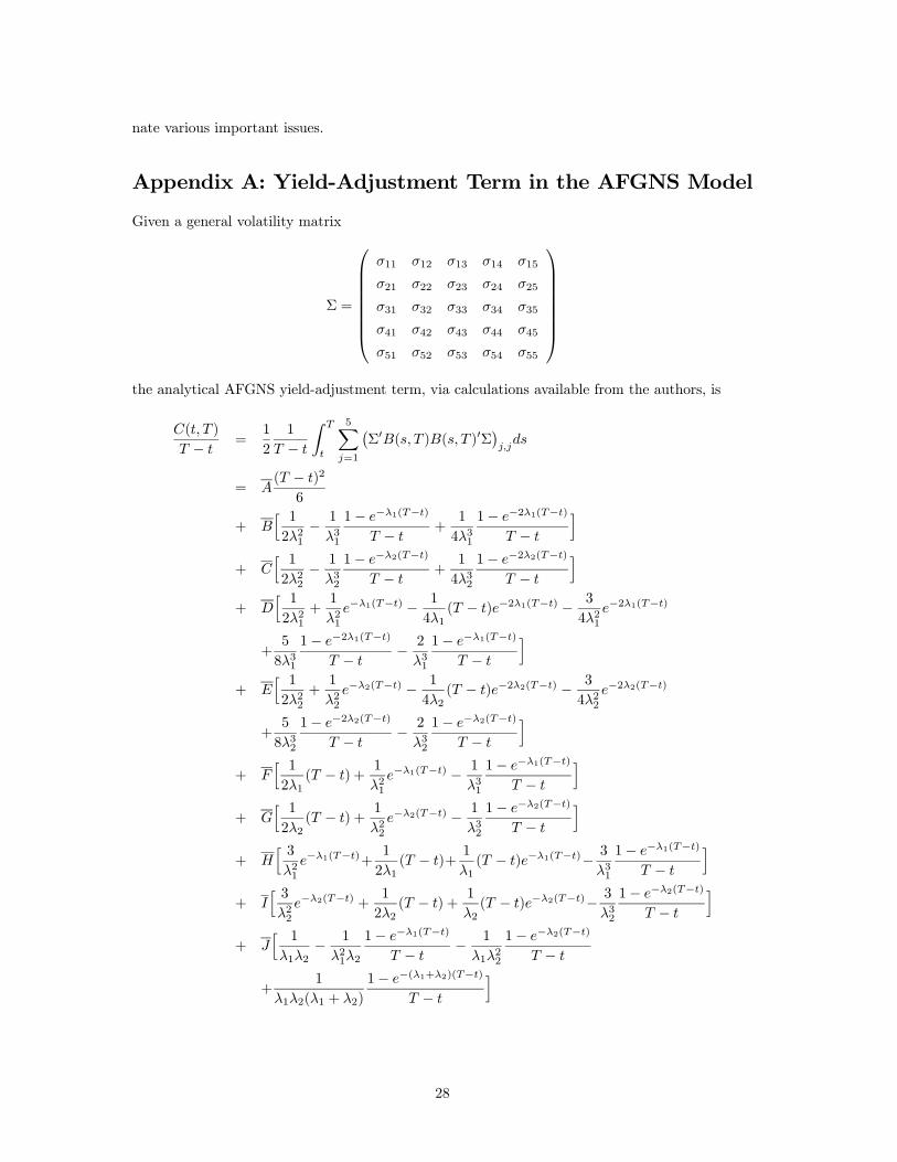
Appendix A: Yield-Adjustment Term in the AFGNS Model

Given a general volatility matrix

Σ =

⎛⎜⎜⎜⎜⎜⎜⎜⎝

σ11 σ12 σ13 σ14 σ15

σ21 σ22 σ23 σ24 σ25

σ31 σ32 σ33 σ34 σ35

σ41 σ42 σ43 σ44 σ45

σ51 σ52 σ53 σ54 σ55

⎞⎟⎟⎟⎟⎟⎟⎟⎠the analytical AFGNS yield-adjustment term, via calculations available from the authors, is

C(t, T )

T − t=

1

2

1

T − t

Z T

t

5Xj=1

¡Σ0B(s, T )B(s, T )0Σ

¢j,jds

= A(T − t)2

6

+ Bh 12λ21− 1

λ31

1− e−λ1(T−t)

T − t+

1

4λ31

1− e−2λ1(T−t)

T − t

i+ C

h 12λ22− 1

λ32

1− e−λ2(T−t)

T − t+

1

4λ32

1− e−2λ2(T−t)

T − t

i+ D

h 12λ21

+1

λ21e−λ1(T−t) − 1

4λ1(T − t)e−2λ1(T−t) − 3

4λ21e−2λ1(T−t)

+5

8λ31

1− e−2λ1(T−t)

T − t− 2

λ31

1− e−λ1(T−t)

T − t

i+ E

h 12λ22

+1

λ22e−λ2(T−t) − 1

4λ2(T − t)e−2λ2(T−t) − 3

4λ22e−2λ2(T−t)

+5

8λ32

1− e−2λ2(T−t)

T − t− 2

λ32

1− e−λ2(T−t)

T − t

i+ F

h 12λ1

(T − t) +1

λ21e−λ1(T−t) − 1

λ31

1− e−λ1(T−t)

T − t

i+ G

h 12λ2

(T − t) +1

λ22e−λ2(T−t) − 1

λ32

1− e−λ2(T−t)

T − t

i+ H

h 3λ21

e−λ1(T−t)+1

2λ1(T − t)+

1

λ1(T − t)e−λ1(T−t)− 3

λ31

1− e−λ1(T−t)

T − t

i+ I

h 3λ22

e−λ2(T−t) +1

2λ2(T − t) +

1

λ2(T − t)e−λ2(T−t)− 3

λ32

1− e−λ2(T−t)

T − t

i+ J

h 1

λ1λ2− 1

λ21λ2

1− e−λ1(T−t)

T − t− 1

λ1λ22

1− e−λ2(T−t)

T − t

+1

λ1λ2(λ1 + λ2)

1− e−(λ1+λ2)(T−t)

T − t

i

28

+ Kh 1λ21+1

λ21e−λ1(T−t) − 1

2λ21e−2λ1(T−t) − 3

λ31

1− e−λ1(T−t)

T − t

+3

4λ31

1− e−2λ1(T−t)

T − t

i+ L

h 1

λ1λ2+

1

λ1λ2e−λ2(T−t) − 1

λ1(λ1 + λ2)e−(λ1+λ2)(T−t)

− 1

λ21λ2

1− e−λ1(T−t)

T − t− 2

λ1λ22

1− e−λ2(T−t)

T − t

+λ1 + 2λ2

λ1λ2(λ1 + λ2)2[1− e−(λ1+λ2)(T−t)]

i+ M

h 1

λ1λ2+

1

λ1λ2e−λ1(T−t) − 1

λ2(λ1 + λ2)e−(λ1+λ2)(T−t)

− 1

λ1λ22

1− e−λ2(T−t)

T − t− 2

λ21λ2

1− e−λ1(T−t)

T − t

+λ2 + 2λ1

λ1λ2(λ1 + λ2)2[1− e−(λ1+λ2)(T−t)]

i+ N

h 1λ22+1

λ22e−λ2(T−t) − 1

2λ22e−2λ2(T−t) − 3

λ32

1− e−λ2(T−t)

T − t

+3

4λ32

1− e−2λ2(T−t)

T − t

i+ O

h 1

λ1λ2+

1

λ1λ2e−λ1(T−t) +

1

λ1λ2e−λ2(T−t)

−³ 1λ1+1

λ2

´ 1

λ1 + λ2e−(λ1+λ2)(T−t) − 2

(λ1 + λ2)2e−(λ1+λ2)(T−t)

− 1

λ1 + λ2(T − t)e−(λ1+λ2)(T−t)

− 2

λ21λ2

1− e−λ1(T−t)

T − t− 2

λ1λ22

1− e−λ2(T−t)

T − t

+2

(λ1 + λ2)31− e−(λ1+λ2)(T−t)

T − t

+³ 1λ1+1

λ2

´ 1

(λ1 + λ2)21− e−(λ1+λ2)(T−t)

T − t

+1

λ1λ2(λ1 + λ2)

1− e−(λ1+λ2)(T−t)

T − t

i,

where

• A = σ211 + σ212 + σ213 + σ214 + σ215,

• B = σ221 + σ222 + σ223 + σ224 + σ225,

• C = σ231 + σ232 + σ233 + σ234 + σ235,

• D = σ241 + σ242 + σ243 + σ244 + σ245,

• E = σ251 + σ252 + σ253 + σ254 + σ255,

• F = σ11σ21 + σ12σ22 + σ13σ23 + σ14σ24 + σ15σ25,

29

• G = σ11σ31 + σ12σ32 + σ13σ33 + σ14σ34 + σ15σ35,

• H = σ11σ41 + σ12σ42 + σ13σ43 + σ14σ44 + σ15σ45,

• I = σ11σ51 + σ12σ52 + σ13σ53 + σ14σ54 + σ15σ55,

• J = σ21σ31 + σ22σ32 + σ23σ33 + σ24σ34 + σ25σ35,

• K = σ21σ41 + σ22σ42 + σ23σ43 + σ24σ44 + σ25σ45,

• L = σ21σ51 + σ22σ52 + σ23σ53 + σ24σ54 + σ25σ55,

• M = σ31σ41 + σ32σ42 + σ33σ43 + σ34σ44 + σ35σ45,

• N = σ31σ51 + σ32σ52 + σ33σ53 + σ34σ54 + σ35σ55,

• O = σ41σ51 + σ42σ52 + σ43σ53 + σ44σ54 + σ45σ55.

Empirically, we can only identify the 15 terms (A,B,C,D,E, F ,G,H, I, J,K,L,M,N,

O). Thus, not all 25 volatility parameters can be identified. This implies that the maximally

flexible specification that is well identified has a volatility matrix given by a triangular volatility

matrix12

Σ =

⎛⎜⎜⎜⎜⎜⎜⎜⎝

σ11 0 0 0 0

σ21 σ22 0 0 0

σ31 σ32 σ33 0 0

σ41 σ42 σ43 σ44 0

σ51 σ52 σ53 σ54 σ55

⎞⎟⎟⎟⎟⎟⎟⎟⎠.

12Note that it can be either upper or lower triangular. The choice is irrelevant for the fit of the model.

30

ReferencesAlmeida, C. and J. Vicente (2008). The Role of No-Arbitrage in Forecasting: Lessons from a

Parametric Term Structure Model. Forthcoming Journal of Banking and Finance.

Bank for International Settlements (2005). Zero-Coupon Yield Curves: Technical Documenta-

tion. BIS papers, No. 25.

Björk, T. and B. J. Christensen (1999). Interest Rate Dynamics and Consistent Forward Rate

Curves. Mathematical Finance 9, 323—48.

Bowsher, C. G. and R. Meeks (2008). The Dynamics of Economic Functions: Modelling and

Forecasting the Yield Curve. Forthcoming Journal of the American Statistical Association.

Christensen, J. H., F. X. Diebold, and G. D. Rudebusch (2007). The Affine Arbitrage-Free Class

of Nelson-Siegel Term Structure Models. Working Paper No. 13611, NBER.

Christensen, J. H., J. A. Lopez, and G. D. Rudebusch (2008a). Inflation Expectations and Risk

Premiums in an Arbitrage-Free Model of Nominal and Real Bond Yields. Unpublished

manuscript, Federal Reserve Bank of San Francisco.

Christensen, J. H., J. A. Lopez, and G. D. Rudebusch (2008b). Do Central Bank Liquidity

Facilities Affect Interbank Lending Rates? Unpublished manuscript, Federal Reserve Bank

of San Francisco.

Christensen, J. H., J. A. Lopez, and G. D. Rudebusch (2008c). Stochastic Volatility in Arbitrage-

Free Nelson-Seigel Models of the Term Sturcture. Unpublished manuscript, Federal Reserve

Bank of San Francisco.

Coroneo, L., K. Nyholm, and R. Vidova-Koleva (2008). How Arbitrage-Free is the Nelson-Siegel

Model? Working Paper No. 874, European Central Bank.

Dai, Q. and K. Singleton (2000). Specification Analysis of Affine Term Structure Models. Journal

of Finance 55, 1943—78.

De Pooter, M. (2007). Examining the Nelson-Siegel Class of Term Structure Models. Discussion

Papers No. 43, Tinbergen Institute.

Diebold, F. X. and C. Li (2006). Forecasting the Term Structure of Government Bond Yields.

Journal of Econometrics 130, 337—64.

Diebold, F. X., M. Piazzesi, and G. D. Rudebusch (2005). Modeling Bond Yields in Finance and

Macroeconomics. American Economic Review 95, 415—20.

Diebold, F. X., G. D.Rudebusch, and S. B. Aruoba (2006). The Macroeconomy and the Yield

Curve: A Dynamic Latent Factor Approach. Journal of Econometrics 131, 309—38.

Duffee, G. (2002). Term Premia and Interest Rate Forecasts in Affine Models. Journal of

Finance 57, 405—43.

31

Filipovic, D. (1999). A Note on the Nelson-Siegel Family. Mathematical Finance 9, 349—59.

Gürkaynak, R., B. Sack, and J. H. Wright (2007). The U.S. Treasury Yield Curve: 1961 to the

Present. Journal of Monetary Economics 54, 2291—304.

Gürkaynak, R., B. Sack, and J. H. Wright (2008). The TIPS Yield Curve and Inflation Com-

pensation. Finance and Economics Discussion Series, No. 2008-05. Board of Governors of

the Federal Reserve System.

Harvey, A. C. (1989). Forecasting, structural time series models and the Kalman filter. Cam-

bridge: Cambridge University Press.

Kim, D. H. and A. Orphanides (2005). Term Structure Estimation with Survey Data on Interest

Rate Forecasts. Finance and Economics Discussion Series, No. 2005-48. Board of Governors

of the Federal Reserve System.

Nelson, C. R. and A. F. Siegel (1987). Parsimonious Modeling of Yield Curves. Journal of

Business 60, 473—89.

Rudebusch, G. D. and T. Wu (2007). Accounting for a Shift in Term Structure Behavior with

No-Arbitrage and Macro-Finance Models. Journal of Money, Credit, and Banking 39,

395—422.

Rudebusch, G. D. and T. Wu (2008). A Macro-Finance Model of the Term Structure, Monetary

Policy, and the Economy. Economic Journal 118, 906—926.

Söderlind, P. and L. E. O. Svensson, (1997). New Techniques to Extract Market Expectations

From Financial Instruments. Journal of Monetary Economics 40, 383—429.

Svennson, L. E. O. (1995). Estimating Forward Interest Rates with the Extended Nelson-Siegel

Method. Quarterly Review , Sveriges Riksbank. 13—26.

32