STUDY OF BOUNDARY LAYER PARAMETERS ON A …ethesis.nitrkl.ac.in/1848/1/gyana.10601032.pdf · STUDY...
50
~ 1 ~ . STUDY OF BOUNDARY LAYER PARAMETERS ON A FLAT PLATE USING WIND TUNNEL A REPORT SUBMITTED IN PARTIAL FULFILLMENT OF THE REQUIREMENTS FOR THE DEGREE OF Bachelor of Technology In Civil Engineering By GYANARANJAN MOHANTY DEPARTMENT OF CIVIL ENGINEERING NIT ROURKELA
Transcript of STUDY OF BOUNDARY LAYER PARAMETERS ON A …ethesis.nitrkl.ac.in/1848/1/gyana.10601032.pdf · STUDY...

~ 1 ~
.
STUDY OF BOUNDARY LAYER PARAMETERS ON A FLAT PLATE USING
WIND TUNNEL
A REPORT SUBMITTED IN PARTIAL FULFILLMENT OF THE REQUIREMENTS FOR THE DEGREE OF
Bachelor of Technology In
Civil Engineering
By
GYANARANJAN MOHANTY
DEPARTMENT OF CIVIL ENGINEERING NIT ROURKELA
~ 2 ~
STUDY OF BOUNDARY LAYER PARAMETERS ON A FLAT PLATE USING
WIND TUNNEL
A REPORT SUBMITTED IN PARTIAL FULFILLMENT OF THE REQUIREMENTS FOR THE DEGREE OF
Bachelor of Technology
In Civil Engineering
By
GYANARANJAN MOHANTY
Under the Guidance of
Prof. A. KUMAR
DEPARTMENT OF CIVIL ENGINEERING
NATIONAL INSTITUTE OF TECHNOLOGY ROURKELA
2010
~ 3 ~
National Institute of Technology
Rourkela
CERTIFICATE
This is to certify that the thesis entitled, “STUDY OF BOUNDARY LAYER PARAMETERS ON A FLAT PLATE USING WIND TUNNEL” submitted by GYANARANJAN MOHANTY in partial fulfillments for the award of Bachelor Of Technology Degree in Civil Engineering at National Institute of Technology, Rourkela (Deemed University) is an authentic work carried out by him under my supervision and guidance.
To the best of my knowledge, the matter embodied in this report has not been
submitted to any other University / Institute for the award of any Certificate.
Date: 12-05-2010
Prof. A.KUMAR Dept. of Civil Engineering
National Institute of Technology Rourkela - 769008

~ 4 ~
ACKNOWLEDGEMENT
I would like to express my deepest gratitude to my guide and motivator
Prof.A.KUMAR, Professor, Civil Engineering Department, National Institute of
Technology, Rourkela for his valuable guidance, sympathy and co-operation for
providing necessary facilities and sources during the entire period of this project.
I wish to convey my sincere gratitude to N.I.T Rourkela authorities for allowing me
to carry out the work and all the faculties of Civil Engineering Department who have
enlightened me during my project.
I am also thankful to the Geotechnical Engineering Laboratory, NIT Rourkela for
helping me during the experiments.
Date: 12th May, 2010 GYANARANJAN MOHANTY

~ 5 ~
CONTENTS
CHAPTER 1: INTRODUCTION……………………………………………………………7
1.1 INTRODUCTION………………………………………………………………………….8
CHAPTER 2: LITERATURE REVIEW…………………………………………………..11
2.1 CONCEPT OF BOUNDARY LAYER…………………………………………………..12
CHAPTER 3: TEST APPARATUS………………………………………………………..14
3.1 WIND TUNNEL………………………………………………………………………….15
3.2 PITOT TUBE……………………………………………………………………………...17
3.4 THE MULTITUBEMANOMETER (AF10A)…………………………………………....18
3.5 GLASS PLATE…………………………………………………………………………...19
3.6 STAND…………………………………………………………………………………....19
CHAPTER 4: TEST PROCEDURE……………………………………………………….20
4.1 TEST PROCEDURE……………………………………………………………………...21
CHAPTER 5: OBSERVATIONS AND CALCULATION…………………………….....22
5.1 EXPERIMENTAL DATAS……………………………………………………………....23
5.2 EFFECTIVE CENTER……………………………………………………………………24
5.3 FREE STREAM VELOCITY…………………………………………………………….24
5.4 REYNOLDS NUMBER…………………………………………………………………..25
5.5 DISPLACEMENT THICKNESS………………………………………………………....25
5.6 MOMENTUM THICKNESS……………………………………………………………...25
5.7 TABLES AND GRAPHS……………………………………………………………........26
CHAPTER 6: DISCUSSIONS AND RESULTS…………………………………………..45
CHAPTER 7: CONCLUSIONS…………………………………………………………….47
CHAPTER 8: REFERENCES……………………………………………………………...49

~ 6 ~
Abstract
For the basic understanding of flow characteristics over a flat smooth plate, the experiment was
carried out in the laboratory using wind tunnel. Readings of the boundary layer were taken at 15
locations over the flat plate (glass surface) with a free stream velocity (U) which varies from
13.4to 13.5 giving Reynolds number corresponding to laminar through turbulent flows. The
height of the boundary layer ranges from 2mm to 29 mm .then the parameters like displacement
thickness and momentum thickness were calculated from the velocity profile. The boundary
layer growth over the glass plate was found out with the help of velocity profiles at different
locations. The boundary layer growth gives a brief idea of fluid flow over a flat surface.

~ 7 ~
Chapter 1
INTRODUCTION
~ 8 ~
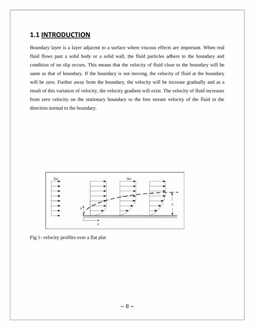
1.1 INTRODUCTION
Boundary layer is a layer adjacent to a surface where viscous effects are important. When real
fluid flows past a solid body or a solid wall, the fluid particles adhere to the boundary and
condition of no slip occurs. This means that the velocity of fluid close to the boundary will be
same as that of boundary. If the boundary is not moving, the velocity of fluid at the boundary
will be zero. Further away from the boundary, the velocity will be increase gradually and as a
result of this variation of velocity, the velocity gradient will exist. The velocity of fluid increases
from zero velocity on the stationary boundary to the free stream velocity of the fluid in the
direction normal to the boundary.
Fig 1- velocity profiles over a flat plat
~ 9 ~
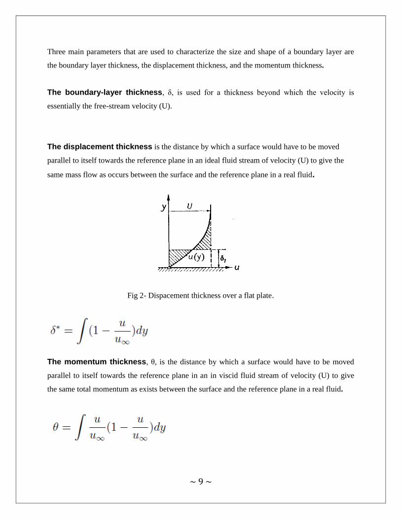
Three main parameters that are used to characterize the size and shape of a boundary layer are
the boundary layer thickness, the displacement thickness, and the momentum thickness.
The boundary-layer thickness, δ, is used for a thickness beyond which the velocity is
essentially the free-stream velocity (U).
The displacement thickness is the distance by which a surface would have to be moved
parallel to itself towards the reference plane in an ideal fluid stream of velocity (U) to give the
same mass flow as occurs between the surface and the reference plane in a real fluid.
Fig 2- Dispacement thickness over a flat plate.
The momentum thickness, θ, is the distance by which a surface would have to be moved
parallel to itself towards the reference plane in an in viscid fluid stream of velocity (U) to give
the same total momentum as exists between the surface and the reference plane in a real fluid.

~ 10 ~
The Reynolds number is a measure of the ratio of inertia forces to viscous forces. It can be used
to characterize flow characteristics over a flat plate. Values under 500,000 are classified as
Laminar flow where values from 500,000 to 1,000,000 are deemed Turbulent flow. Is it
important to distinguish between turbulent and non turbulent flow since the boundary layer
varies.
The factor which characterizes Reynolds numbe Rex is the distance from the leading egde .
Rex =Ux/ʋ
Fig 3- boundary layer over a flat plate.(y scale enlarged)
~ 11 ~
Chapter 2
LITERATURE
REVIEW

~ 12 ~
2.1 CONCEPTS OF BOUNDARY LAYER
DEFINITION OF THICKNESS
The boundary layer thickness δ, as the thickness where the velocity reaches the free stream value
U. The velocity in the boundary layer increases towards U is an asymptotic manner.
The displacement thickness δ* is defined as the thickness by which fluid outside the layer is
displaced away from the boundary by the existence of the layer, by the streamline approaching B
as shown below.
The value of velocity u within the layer is a function of distance y from the boundary as curve
OA. If there was exists no boundary layer, then the free stream velocity U would persist right
down to the boundary (C0).
Fig 4-Boundary layer thickness
~ 13 ~
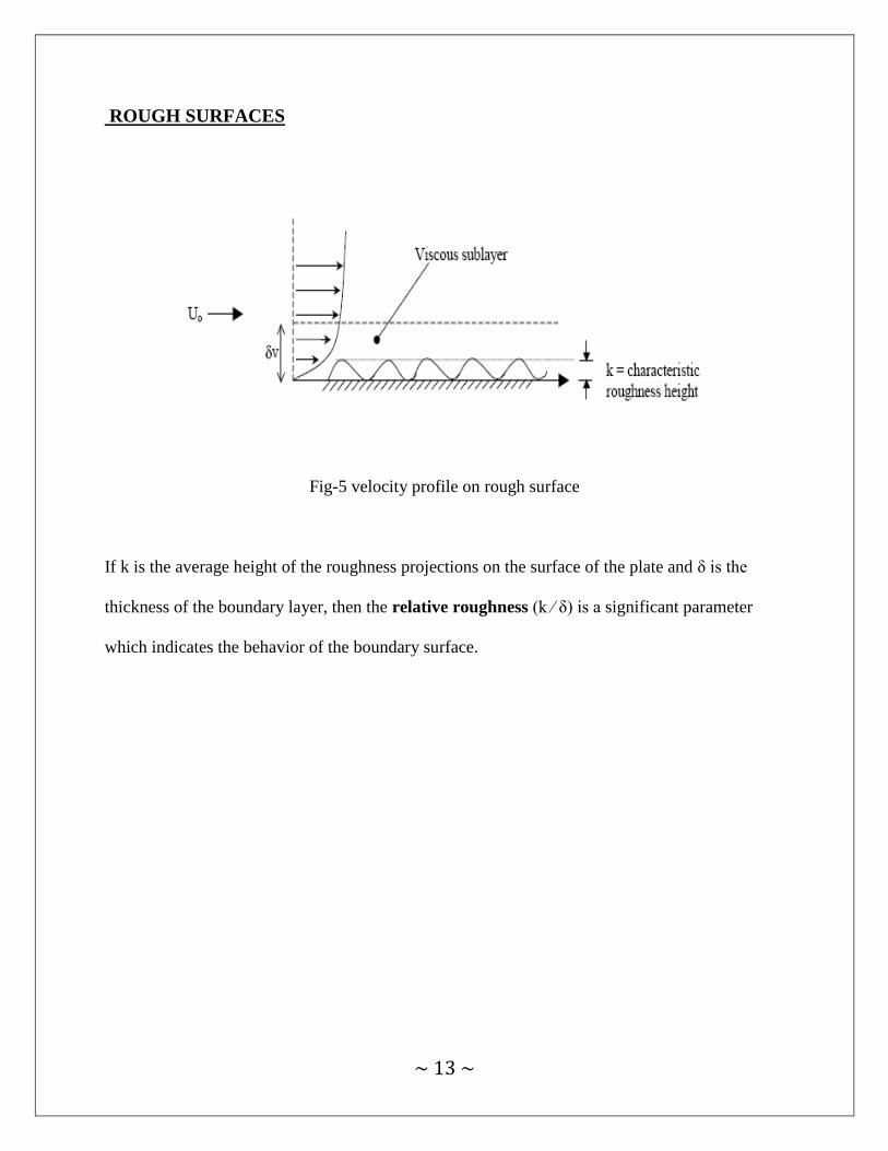
ROUGH SURFACES
Fig-5 velocity profile on rough surface
If k is the average height of the roughness projections on the surface of the plate and δ is the
thickness of the boundary layer, then the relative roughness (k ⁄ δ) is a significant parameter
which indicates the behavior of the boundary surface.

~ 14 ~
Chapter 3
TEST
APPARATUS
~ 15 ~
3.1 WINDTUNNEL
DESCRIPTION
It is a device in form of a long duct for producing a moving airstream for experimental purposes.
It is used to study the effects of air moving past solid objects. The model science has assumed an
important role in engineering. As it is not only makes it possible to study the behavior of the
structure or machines where mathematical methods are impossible, time-consuming or
inaccurate but also results in economy since it is easier and chaper to effect changes in a model
rather than the prototype.
There are four essential components:
EFFUSER:-
This is placed upstream of the working section. In it the fluid is accelerated from rest to
approximately at upstream end to the required conditions at the working section. The effuse
contain a conversing cone, screens and other devises to refuse the turbulence and produce a
uniform airstream at the exit.
WORKING SECTION:-
It is here that the model is placed is placed in the air stream leaving the downstream end of
the effuser and the required observations are made. The working section consists of accessories
to hold the instruments and models and devices for facilitating the motion of the model in all
directions relative to airstream.
DIFFUSER:-
The function of the diffuser is to recover the kinetic energy of the airstream leaving the
working section efficiently as possible.
DRIVING UNIT:-
Power is supplied continuously to maintain the flow through suction (at variable condition).
This is done using a fan or propeller and a motor.
~ 16 ~
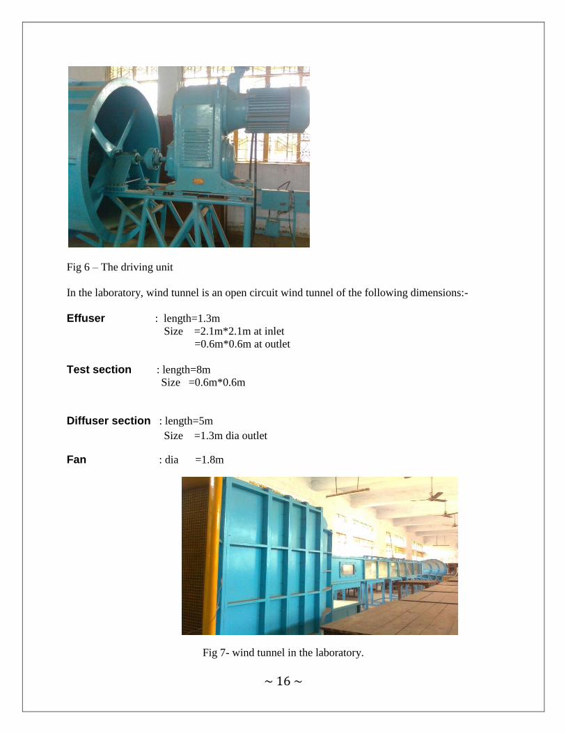
Fig 6 – The driving unit
In the laboratory, wind tunnel is an open circuit wind tunnel of the following dimensions:-
Effuser : length=1.3m
Size =2.1m*2.1m at inlet
=0.6m*0.6m at outlet
Test section : length=8m Size =0.6m*0.6m
Diffuser section : length=5m
Size =1.3m dia outlet
Fan : dia =1.8m
Fig 7- wind tunnel in the laboratory.
~ 17 ~
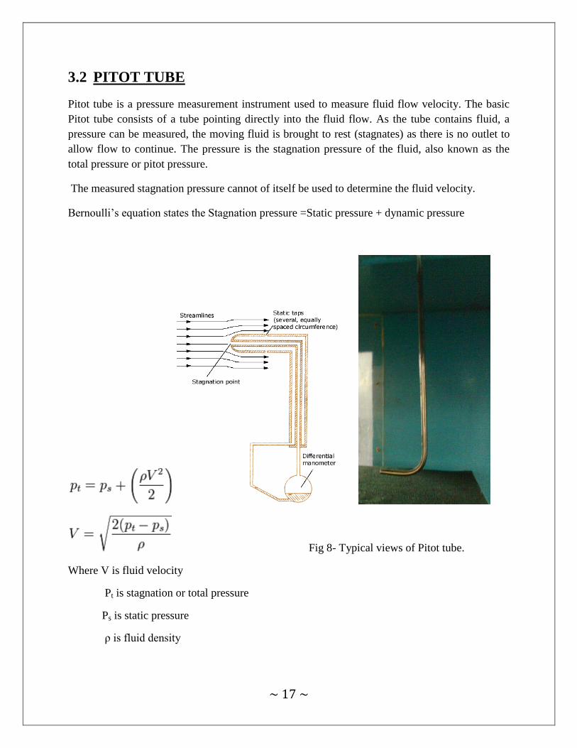
3.2 PITOT TUBE
Pitot tube is a pressure measurement instrument used to measure fluid flow velocity. The basic
Pitot tube consists of a tube pointing directly into the fluid flow. As the tube contains fluid, a
pressure can be measured, the moving fluid is brought to rest (stagnates) as there is no outlet to
allow flow to continue. The pressure is the stagnation pressure of the fluid, also known as the
total pressure or pitot pressure.
The measured stagnation pressure cannot of itself be used to determine the fluid velocity.
Bernoulli’s equation states the Stagnation pressure =Static pressure + dynamic pressure
Fig 8- Typical views of Pitot tube.
Where V is fluid velocity
Pt is stagnation or total pressure
Ps is static pressure
ρ is fluid density
~ 18 ~
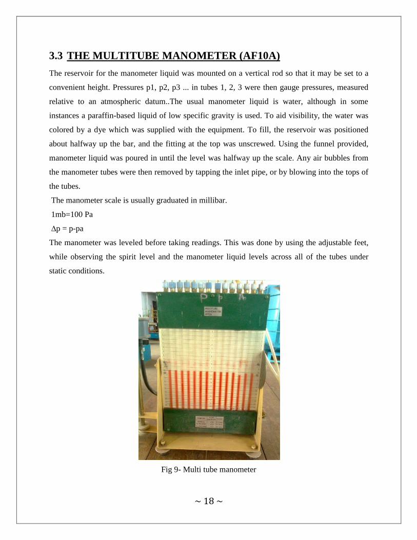
3.3 THE MULTITUBE MANOMETER (AF10A)
The reservoir for the manometer liquid was mounted on a vertical rod so that it may be set to a
convenient height. Pressures p1, p2, p3 ... in tubes 1, 2, 3 were then gauge pressures, measured
relative to an atmospheric datum..The usual manometer liquid is water, although in some
instances a paraffin-based liquid of low specific gravity is used. To aid visibility, the water was
colored by a dye which was supplied with the equipment. To fill, the reservoir was positioned
about halfway up the bar, and the fitting at the top was unscrewed. Using the funnel provided,
manometer liquid was poured in until the level was halfway up the scale. Any air bubbles from
the manometer tubes were then removed by tapping the inlet pipe, or by blowing into the tops of
the tubes.
The manometer scale is usually graduated in millibar.
1mb=100 Pa
∆p = p-pa
The manometer was leveled before taking readings. This was done by using the adjustable feet,
while observing the spirit level and the manometer liquid levels across all of the tubes under
static conditions.
Fig 9- Multi tube manometer

~ 19 ~
3.4 GLASS PLATE:
A smooth flat surface to define a clear leading edge having dimensions:
Length =100cm
Width =50.8cm
Thickness=3mm
3.4 STAND
A stand of required weight to hold the glass in a fixed position inside the test section of the wind
tunnel.
Fig 10-The glass plate on the stand.
~ 20 ~
Chapter 4
TEST
PROCEDURE

~ 21 ~
4. TEST PROCEDURE
1. The flat smooth surface (glass plate) was kept on a stand firmly, at the test section of the wind
tunnel as shown below.
2. The wind tunnel was set up with a Pitot tube placed at 20 cm from the leading edge, attached
to a multi-tube manometer to get the pressure differentials.
3. Then the wind tunnel was turned on, and the manometer was calibrated.
4. The pressure differentials readings were taken at 22 points within the boundary layer gradually
Increasing ∆y (distance measured from the surface) from 1mm to 5mm.
5. The pressure difference was noted carefully,
6. The test was repeated adjusting the pitot tube at 25, 30, 35, 40, 45, 50, 55, 60, 65, 70, 75, 80,
85, 90, 95, 100 cm from the leading edge of the glass plate.
Fig 11- The experimental set up.
~ 22 ~
Chapter 5
OBSERVATONS
AND
CALCULATIONS
~ 23 ~
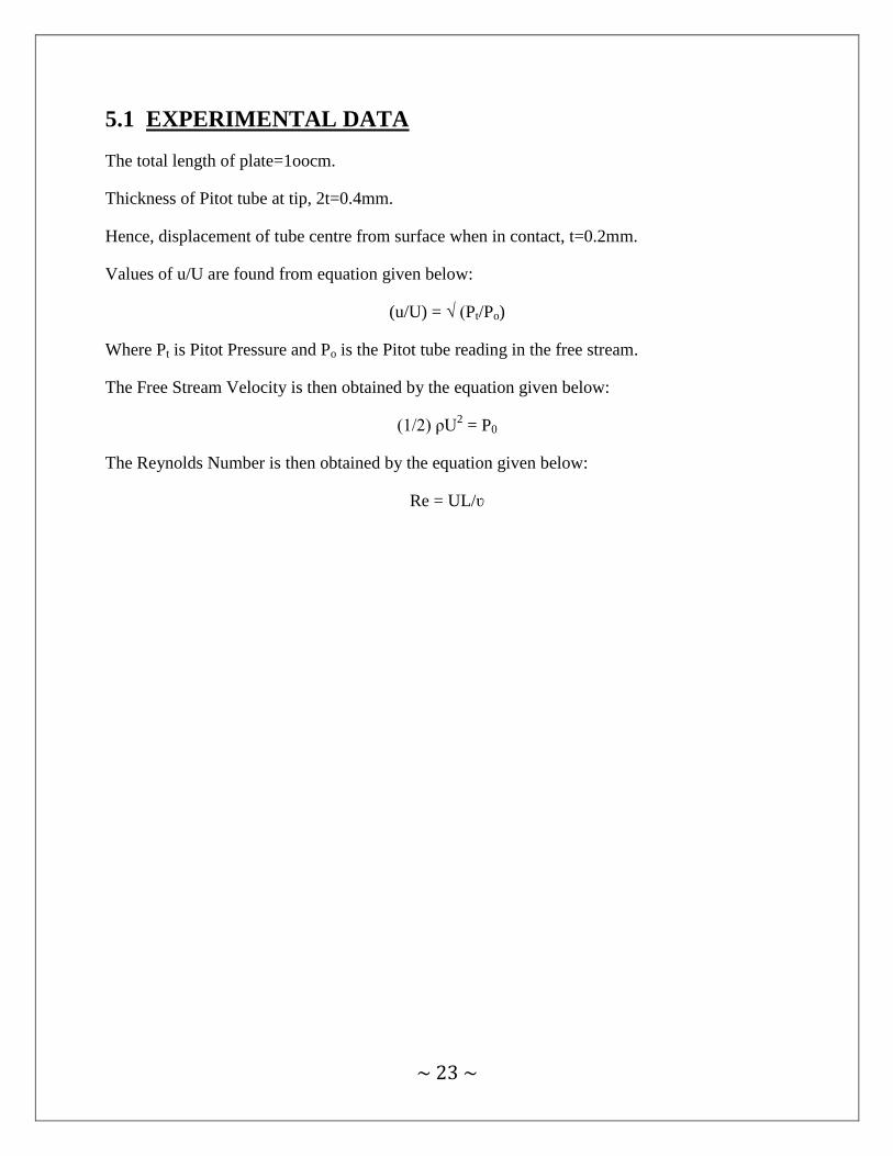
5.1 EXPERIMENTAL DATA
The total length of plate=1oocm.
Thickness of Pitot tube at tip, 2t=0.4mm.
Hence, displacement of tube centre from surface when in contact, t=0.2mm.
Values of u/U are found from equation given below:
(u/U) = √ (Pt/Po)
Where Pt is Pitot Pressure and Po is the Pitot tube reading in the free stream.
The Free Stream Velocity is then obtained by the equation given below:
(1/2) ρU2 = P0
The Reynolds Number is then obtained by the equation given below:
Re = UL/ʋ

~ 24 ~
The basic assumptions used in the following calculations are:
1. The working fluid, air, was an incompressible fluid as the testing was done in the low
speed wind tunnel.
2. A standard atmospheric condition of the air is assumed.
Table 1-Nomenclature:
ρ Air density
u Velocity at sections
U Free stream velocity
ʋ Kinematic viscosity
µ Dynamic viscosity
∆P Pressure difference
L Length of the plate
y Distance from the surface
Re Reynolds number
x Distance from the leading edge
ᵟ Boundary thickness
ᵟ* Displacement thickness
θ
Momentum thickness
5.2 EFFECTIVE CENTRE
The effective center equation is used to measure the first ∆y distance on which data is taken at
each location.
Thickness of Pitot tube at tip, 2t=0.4mm.
Hence, displacement of tube centre from surface when in contact, t=0.2mm
5.3 FREE STREAM VELOCITY
The reading recorded were in millibar pressure was converted to Pascal .the free stream velocity
requires Pascal pressure which was calculated .the free steram velocity was found out with the
use of formula.
U=√ (2*∆P/ ρair)
Applying the above formula, the free stream velocity was calculated as 13.44m/s.

~ 25 ~
5.4 REYNOLDS NUMBER
After calculating the free stream velocity at all the sections of the plate,the Reynolds number was
determined using the formula.
Re = ρx
µ
The distance from the leading edge was measured at which boundary layer distributions were
evaluated and given in the Table
5.5 DISPLACEMENT THICKNESS
The displacement thickness at all the points of the pitot tube is given by the equation().After
getting the free stream velocity and the velocity at different y distance from the surface,
displacement thickness was calculated. The following formula is used to get a linear
approximation of the displacement thickness at all Pitot tube locations:
ᵟ = ∑ (1-u/U) ∆y
5.6 MOMENTUM THICKNESS
The momentum thickness at all the locations of the Pitot tube is given by the equation()
The linear approximation of momentum thickness was calculated using the formula:
θ =∑ (u/U) (1-u/U) ∆y
~ 26 ~
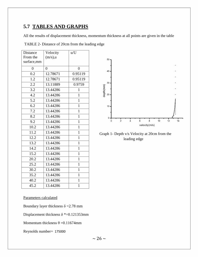
5.7 TABLES AND GRAPHS
All the results of displacement thickness, momentum thickness at all points are given in the table
TABLE 2- Distance of 20cm from the leading edge
Graph 1- Depth v/s Velocity at 20cm from the
leading edge
Parameters calculated
Boundary layer thickness δ =2.78 mm
Displacement thickness δ *=0.121353mm
Momentum thickness θ =0.11674mm
Reynolds number= 175000
Distance
From the
surface,mm
Velocity
(m/s),u
u/U
0 0 0
0.2 12.78671 0.95119
1.2 12.78671 0.95119
2.2 13.11889 0.9759
3.2 13.44286 1
4.2 13.44286 1
5.2 13.44286 1
6.2 13.44286 1
7.2 13.44286 1
8.2 13.44286 1
9.2 13.44286 1
10.2 13.44286 1
11.2 13.44286 1
12.2 13.44286 1
13.2 13.44286 1
14.2 13.44286 1
15.2 13.44286 1
20.2 13.44286 1
25.2 13.44286 1
30.2 13.44286 1
35.2 13.44286 1
40.2 13.44286 1
45.2 13.44286 1
~ 27 ~
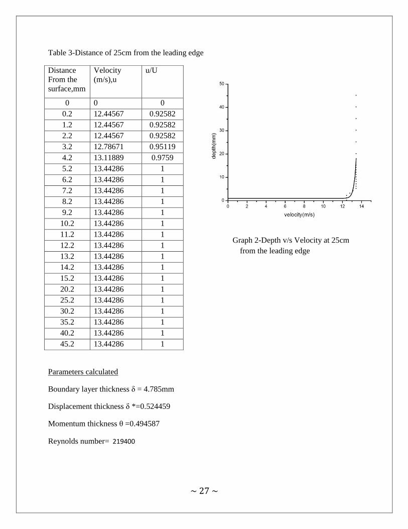
Table 3-Distance of 25cm from the leading edge
Graph 2-Depth v/s Velocity at 25cm
from the leading edge
Parameters calculated
Boundary layer thickness δ = 4.785mm
Displacement thickness δ *=0.524459
Momentum thickness θ =0.494587
Reynolds number= 219400
Distance
From the
surface,mm
Velocity
(m/s),u
u/U
0 0 0
0.2 12.44567 0.92582
1.2 12.44567 0.92582
2.2 12.44567 0.92582
3.2 12.78671 0.95119
4.2 13.11889 0.9759
5.2 13.44286 1
6.2 13.44286 1
7.2 13.44286 1
8.2 13.44286 1
9.2 13.44286 1
10.2 13.44286 1
11.2 13.44286 1
12.2 13.44286 1
13.2 13.44286 1
14.2 13.44286 1
15.2 13.44286 1
20.2 13.44286 1
25.2 13.44286 1
30.2 13.44286 1
35.2 13.44286 1
40.2 13.44286 1
45.2 13.44286 1
~ 28 ~
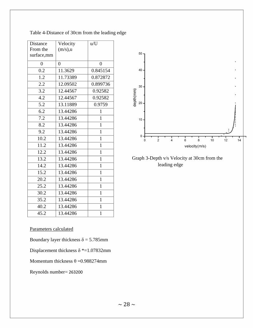
Table 4-Distance of 30cm from the leading edge
Graph 3-Depth v/s Velocity at 30cm from the
leading edge
Parameters calculated
Boundary layer thickness δ = 5.785mm
Displacement thickness δ *=1.07832mm
Momentum thickness θ =0.988274mm
Reynolds number= 263200
Distance
From the
surface,mm
Velocity
(m/s),u
u/U
0 0 0
0.2 11.3629 0.845154
1.2 11.73389 0.872872
2.2 12.09502 0.899736
3.2 12.44567 0.92582
4.2 12.44567 0.92582
5.2 13.11889 0.9759
6.2 13.44286 1
7.2 13.44286 1
8.2 13.44286 1
9.2 13.44286 1
10.2 13.44286 1
11.2 13.44286 1
12.2 13.44286 1
13.2 13.44286 1
14.2 13.44286 1
15.2 13.44286 1
20.2 13.44286 1
25.2 13.44286 1
30.2 13.44286 1
35.2 13.44286 1
40.2 13.44286 1
45.2 13.44286 1

~ 29 ~
Table 5-Distance of 35cm from the leading edge
Graph 4-Depth v/s Velocity at 35cm from
the leading edge
Parameters calculated
Boundary layer thickness δ =7.78mm
Displacement thickness δ *=2.072192mm
Momentum thickness θ =1.880188mm
Reynolds number= 307000
Distance
From the
surface,mm
Velocity
(m/s),u
u/U
0 0 0
0.2 11.36129 0.845154
1.2 12.09502 0.899735
2.2 11.36129 0.845154
3.2 11.73389 0.872872
4.2 12.44567 0.92582
5.2 12.44567 0.92582
6.2 13.11889 0.95119
7.2 13.44286 0.9759
8.2 13.44286 1
9.2 13.44286 1
10.2 13.44286 1
11.2 13.44286 1
12.2 13.44286 1
13.2 13.44286 1
14.2 13.44286 1
15.2 13.44286 1
20.2 13.44286 1
25.2 13.44286 1
30.2 13.44286 1
35.2 13.44286 1
40.2 13.44286 1
45.2 13.44286 1
~ 30 ~
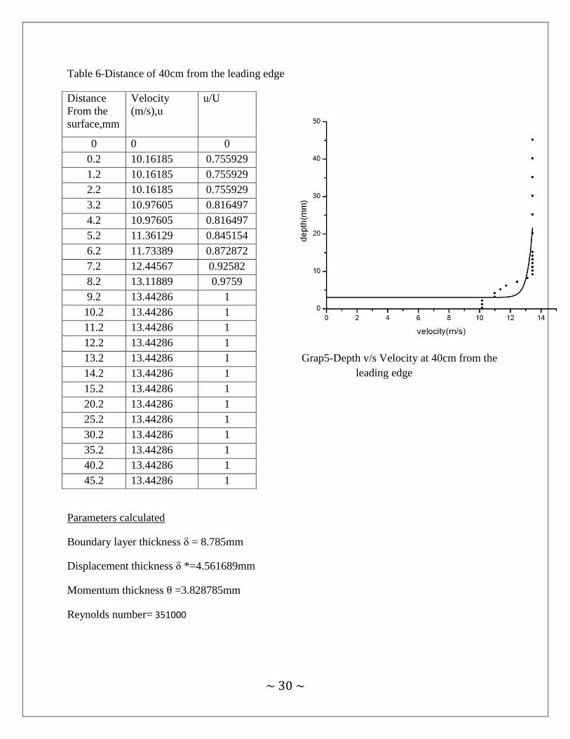
Table 6-Distance of 40cm from the leading edge
Grap5-Depth v/s Velocity at 40cm from the
leading edge
Parameters calculated
Boundary layer thickness δ = 8.785mm
Displacement thickness δ *=4.561689mm
Momentum thickness θ =3.828785mm
Reynolds number= 351000
Distance
From the
surface,mm
Velocity
(m/s),u
u/U
0 0 0
0.2 10.16185 0.755929
1.2 10.16185 0.755929
2.2 10.16185 0.755929
3.2 10.97605 0.816497
4.2 10.97605 0.816497
5.2 11.36129 0.845154
6.2 11.73389 0.872872
7.2 12.44567 0.92582
8.2 13.11889 0.9759
9.2 13.44286 1
10.2 13.44286 1
11.2 13.44286 1
12.2 13.44286 1
13.2 13.44286 1
14.2 13.44286 1
15.2 13.44286 1
20.2 13.44286 1
25.2 13.44286 1
30.2 13.44286 1
35.2 13.44286 1
40.2 13.44286 1
45.2 13.44286 1

~ 31 ~
Table 7-Distance of 45cm from the leading edge
Graph 6-Depth v/s Velocity at 45cm from the
leading edge
Parameters calculated
Boundary layer thickness δ = 9.78mm
Displacement thickness δ *=3.396277mm
Momentum thickness θ =3.05134mm
Reynolds number= 394000
Distance
From the
surface,mm
Velocity
(m/s),u
u/U
0 0 0
0.2 10.97605 0.816497
1.2 10.97605 0.816497
2.2 10.97605 0.816497
3.2 11.36129 0.845154
4.2 12.09502 0.899735
5.2 12.44567 0.92582
6.2 12.44567 0.92582
7.2 12.78671 0.95119
8.2 12.78671 0.95119
9.2 13.11889 0.9759
10.2 13.44286 1
11.2 13.44286 1
12.2 13.44286 1
13.2 13.44286 1
14.2 13.44286 1
15.2 13.44286 1
20.2 13.44286 1
25.2 13.44286 1
30.2 13.44286 1
35.2 13.44286 1
40.2 13.44286 1
45.2 13.44286 1

~ 32 ~
Table 8-Distance of 50cm from the leading edge
Graph 7-Depth v/s Velocity at 50cm from
the leading edge
Parameters calculated
Boundary layer thickness δ = 9.785mm
Displacement thickness δ *=4.7449123mm
Momentum thickness θ =4.108018mm
Reynolds number= 438800
Distance
From the
surface,mm
Velocity
(m/s),u
u/U
0 0 0
0.2 11.36129 0.845154
1.2 11.36129 0.845154
2.2 10.97605 0.816497
3.2 10.97605 0.816497
4.2 10.97605 0.816497
5.2 11.36129 0.845154
6.2 12.09502 0.899735
7.2 12.09502 0.899735
8.2 12.78671 0.95119
9.2 13.11889 0.9759
10.2 13.44286 1
11.2 13.44286 1
12.2 13.44286 1
13.2 13.44286 1
14.2 13.44286 1
15.2 13.44286 1
20.2 13.44286 1
25.2 13.44286 1
30.2 13.44286 1
35.2 13.44286 1
40.2 13.44286 1
45.2 13.44286 1

~ 33 ~
Table 9-Distance of 55cm from the leading edge
Graph 8-Depth v/s Velocity at 55cm from the
leading edge
Parameters calculated
Boundary layer thickness δ = 10.78mm
Displacement thickness δ *=4.212919mm
Momentum thickness θ =3.758508mm
Reynolds number= 482650
Distance
From the
surface,mm
Velocity
(m/s),u
u/U
0 0 0
0.2 10.97605 0.816497
1.2 10.97605 0.816497
2.2 10.97605 0.816497
3.2 11.36129 0.845154
4.2 11.73389 0.872872
5.2 11.73389 0.872872
6.2 12.44567 0.92582
7.2 12.44567 0.92582
8.2 12.78671 0.95119
9.2 13.11889 0.9759
10.2 13.11889 0.9759
11.2 13.44286 1
12.2 13.44286 1
13.2 13.44286 1
14.2 13.44286 1
15.2 13.44286 1
20.2 13.44286 1
25.2 13.44286 1
30.2 13.44286 1
35.2 13.44286 1
40.2 13.44286 1
45.2 13.44286 1

~ 34 ~
Table 10-Distance of 60cm from the leading edge
Graph 9-Depth v/s Velocity at 60cm from the
leading edge
Parameters calculated
Boundary layer thickness δ = 12.78mm
Displacement thickness δ *=6.194417mm
Momentum thickness θ =5.50082mm
Reynolds number= 526500
Distance
From the
surface,mm
Velocity
(m/s),u
u/U
0 0 0
0.2 10.57679 0.786796
1.2 10.97605 0.816497
2.2 10.97605 0.816497
3.2 10.97605 0.816497
4.2 11.36129 0.845154
5.2 11.73389 0.872872
6.2 11.73389 0.872872
7.2 12.09502 0.899735
8.2 12.44567 0.92582
9.2 12.78671 0.95119
10.2 12.78671 0.95119
11.2 13.11889 0.9759
12.2 13.11889 0.9759
13.2 13.44286 1
14.2 13.44286 1
15.2 13.44286 1
20.2 13.44286 1
25.2 13.44286 1
30.2 13.44286 1
35.2 13.44286 1
40.2 13.44286 1
45.2 13.44286 1
~ 35 ~
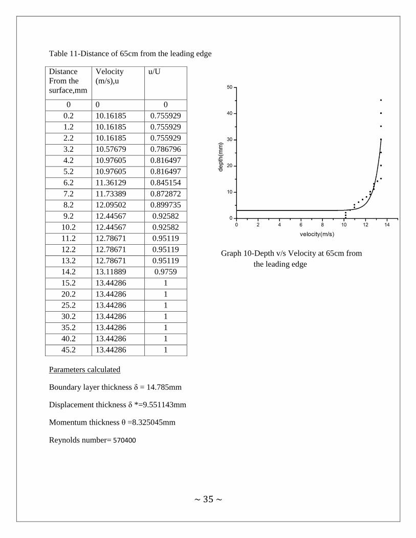
Table 11-Distance of 65cm from the leading edge
Graph 10-Depth v/s Velocity at 65cm from
the leading edge
Parameters calculated
Boundary layer thickness δ = 14.785mm
Displacement thickness δ *=9.551143mm
Momentum thickness θ =8.325045mm
Reynolds number= 570400
Distance
From the
surface,mm
Velocity
(m/s),u
u/U
0 0 0
0.2 10.16185 0.755929
1.2 10.16185 0.755929
2.2 10.16185 0.755929
3.2 10.57679 0.786796
4.2 10.97605 0.816497
5.2 10.97605 0.816497
6.2 11.36129 0.845154
7.2 11.73389 0.872872
8.2 12.09502 0.899735
9.2 12.44567 0.92582
10.2 12.44567 0.92582
11.2 12.78671 0.95119
12.2 12.78671 0.95119
13.2 12.78671 0.95119
14.2 13.11889 0.9759
15.2 13.44286 1
20.2 13.44286 1
25.2 13.44286 1
30.2 13.44286 1
35.2 13.44286 1
40.2 13.44286 1
45.2 13.44286 1
~ 36 ~
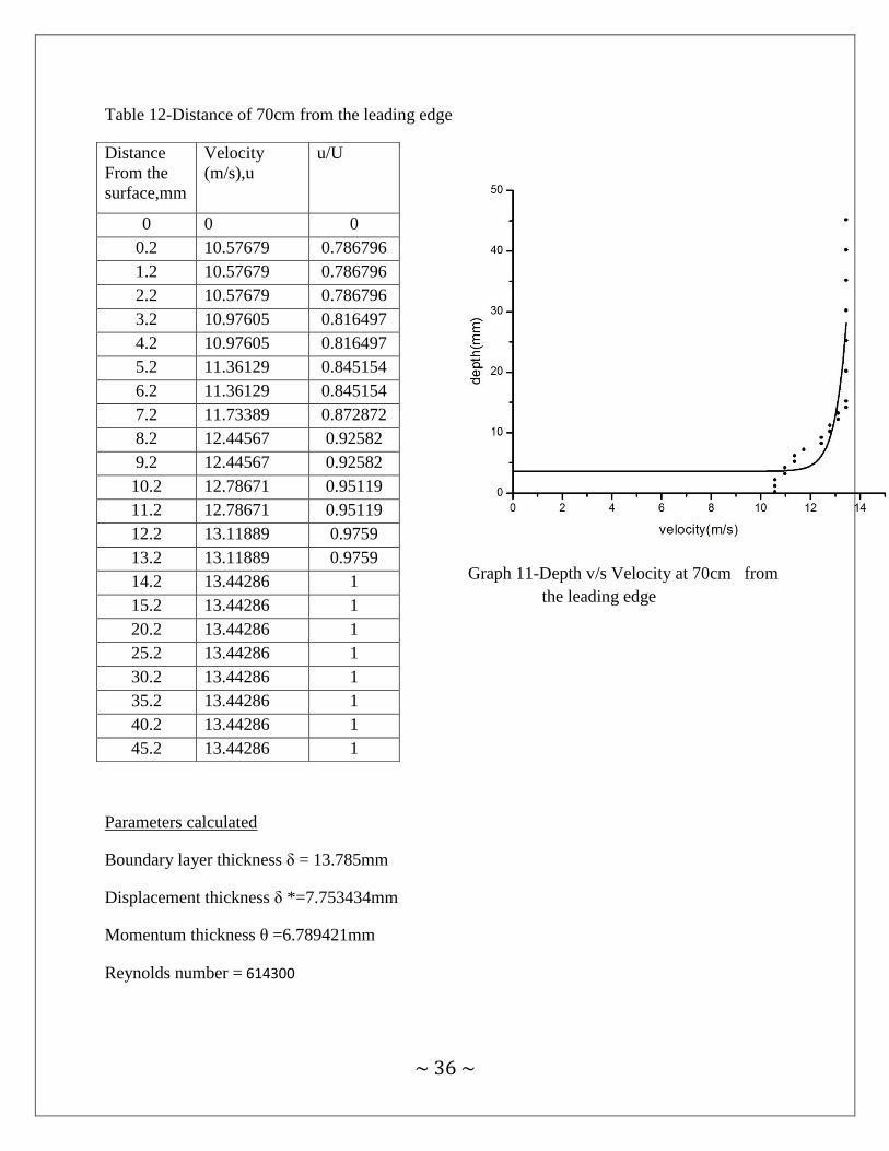
Table 12-Distance of 70cm from the leading edge
Graph 11-Depth v/s Velocity at 70cm from
the leading edge
Parameters calculated
Boundary layer thickness δ = 13.785mm
Displacement thickness δ *=7.753434mm
Momentum thickness θ =6.789421mm
Reynolds number = 614300
Distance
From the
surface,mm
Velocity
(m/s),u
u/U
0 0 0
0.2 10.57679 0.786796
1.2 10.57679 0.786796
2.2 10.57679 0.786796
3.2 10.97605 0.816497
4.2 10.97605 0.816497
5.2 11.36129 0.845154
6.2 11.36129 0.845154
7.2 11.73389 0.872872
8.2 12.44567 0.92582
9.2 12.44567 0.92582
10.2 12.78671 0.95119
11.2 12.78671 0.95119
12.2 13.11889 0.9759
13.2 13.11889 0.9759
14.2 13.44286 1
15.2 13.44286 1
20.2 13.44286 1
25.2 13.44286 1
30.2 13.44286 1
35.2 13.44286 1
40.2 13.44286 1
45.2 13.44286 1
~ 37 ~
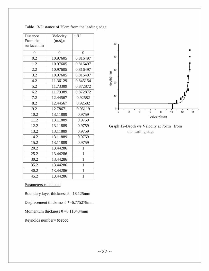
Table 13-Distance of 75cm from the leading edge
Graph 12-Depth v/s Velocity at 75cm from
the leading edge
Parameters calculated
Boundary layer thickness δ =18.125mm
Displacement thickness δ *=6.775278mm
Momentum thickness θ =6.110434mm
Reynolds number= 658000
Distance
From the
surface,mm
Velocity
(m/s),u
u/U
0 0 0
0.2 10.97605 0.816497
1.2 10.97605 0.816497
2.2 10.97605 0.816497
3.2 10.97605 0.816497
4.2 11.36129 0.845154
5.2 11.73389 0.872872
6.2 11.73389 0.872872
7.2 12.44567 0.92582
8.2 12.44567 0.92582
9.2 12.78671 0.95119
10.2 13.11889 0.9759
11.2 13.11889 0.9759
12.2 13.11889 0.9759
13.2 13.11889 0.9759
14.2 13.11889 0.9759
15.2 13.11889 0.9759
20.2 13.44286 1
25.2 13.44286 1
30.2 13.44286 1
35.2 13.44286 1
40.2 13.44286 1
45.2 13.44286 1

~ 38 ~
Table 14-Distance of 80cm from the leading edge
Graph 13-Depth v/s Velocity at 80cm from
the leading edge
Parameters calculated
Boundary layer thickness δ =18.125mm
Displacement thickness δ *=13.11011mm
Momentum thickness θ =11.19465mm
Reynolds number= 702000
Distance
From the
surface,mm
Velocity
(m/s),u
u/U
0 0 0
0.2 10.16185 0.755929
1.2 10.16185 0.755929
2.2 10.16185 0.755929
3.2 10.16185 0.755929
4.2 10.57679 0.786796
5.2 10.57679 0.786796
6.2 10.97605 0.816497
7.2 11.36129 0.845154
8.2 11.36129 0.845154
9.2 11.73389 0.872872
10.2 12.09502 0.899735
11.2 12.09502 0.899735
12.2 12.44567 0.92582
13.2 12.78671 0.95119
14.2 12.78671 0.95119
15.2 13.11889 0.9759
20.2 13.44286 1
25.2 13.44286 1
30.2 13.44286 1
35.2 13.44286 1
40.2 13.44286 1
45.2 13.44286 1

~ 39 ~
Table 15-Distance of 85cm from the leading edge
Graph 14-Depth v/s Velocity at 85cm from
the leading edge
Parameters calculated
Boundary layer thickness δ = 33.125mm
Displacement thickness δ *=17.57433mm
Momentum thickness θ =15.13037mm
Reynolds number= 745900
Distance
From the
surface,mm
Velocity
(m/s),u
u/U
0 0 0
0.2 10.16185 0.755929
1.2 1016185 0.755929
2.2 10.16185 0.755929
3.2 10.16185 0.755929
4.2 10.16185 0.755929
5.2 10.57679 0.786796
6.2 10.57679 0.786796
7.2 10.97605 0.816497
8.2 11.73389 0.872872
9.2 11.73389 0.872872
10.2 11.73389 0.872872
11.2 11.73389 0.872872
12.2 12.09502 0.899736
13.2 12.44567 0.92582
14.2 12.44567 0.92582
15.2 12.44567 0.92582
20.2 13.11889 0.9759
25.2 13.11889 0.9759
30.2 13.11889 0.9759
35.2 13.44286 1
40.2 13.44286 1
45.2 13.44286 1

~ 40 ~
Table 16-Distance of 90cm from the leading edge
Graph 15-Depth v/s Velocity at 90cm from the
leading edge
Parameters calculated
Boundary layer thickness δ = 23.125mm
Displacement thickness δ *=13.72195mm
Momentum thickness θ =11.47798mm
Reynolds number= 789800
Distance
From the
surface,mm
Velocity
(m/s),u
u/U
0 0 0
0.2 9.276456 0.690066
1.2 9.276456 0.690066
2.2 9.276456 0.690066
3.2 9.729229 0.723747
4.2 9.729229 0.723747
5.2 10.57679 0.786796
6.2 10.57679 0.786796
7.2 10.97605 0.816497
8.2 11.73389 0.872872
9.2 11.73389 0.872872
10.2 12.09502 0.899736
11.2 12.44567 0.92582
12.2 12.44567 0.92582
13.2 12.78671 0.95119
14.2 13.11889 0.9759
15.2 13.11889 0.9759
20.2 13.11889 0.9759
25.2 13.44286 1
30.2 13.44286 1
35.2 13.44286 1
40.2 13.44286 1
45.2 13.44286 1

~ 41 ~
Table 17-Distance of 95cm from the leading edge
Graph 16-Depth v/s Velocity at 95cm from the
leading edge
Parameters calculated
Boundary layer thickness δ = 28.125mm
Displacement thickness δ *=17.2343mm
Momentum thickness θ =14.6704mm
Reynolds number= 833600
Distance
From the
surface,mm
Velocity
(m/s),u
u/U
0 0 0
0.2 10.16185 0.755929
1.2 10.16185 0.755929
2.2 10.16185 0.755929
3.2 10.16185 0.755929
4.2 10.16185 0.755929
5.2 10.16185 0.755929
6.2 10.57679 0.786796
7.2 10.97605 0.816497
8.2 11.36129 0.845154
9.2 11.73389 0.872872
10.2 11.73389 0.872872
11.2 11.73389 0.8728720
12.2 12.09502 0.899736
13.2 12.44567 0.92582
14.2 12.44567 0.92582
15.2 12.44567 0.92582
20.2 13.11889 0.9759
25.2 13.11889 0.9759
30.2 13.44286 1
35.2 13.44286 1
40.2 13.44286 1
45.2 13.44286 1

~ 42 ~
Table 18-Distance of 100cm from the leading edge
Graph 17-Depth v/s Velocity at 100cm from the
leading edge
Parameters calculated
Boundary layer thickness δ = 28.125mm
Displacement thickness δ *=17.75434mm
Momentum thickness θ =14.74mm
Reynolds number= 877000
Distance
From the
surface,mm
Velocity
(m/s),u
u/U
0 0 0
0.2 9.729228887 0.723747
1.2 9.729228887 0.723747
2.2 9.729228887 0.723747
3.2 9.729228887 0.723747
4.2 9.729228887 0.723747
5.2 10.16184815 0.755929
6.2 10.5767869 0.786796
7.2 10.5767869 0.786796
8.2 10.5767869 0.786796
9.2 11.36129162 0.845154
10.2 11.36129162 0.845154
11.2 11.73389153 0.872872
12.2 12.44567141 0.92582
13.2 12.44567141 0.92582
14.2 12.78671185 0.95119
15.2 12.78671185 0.95119
20.2 13.11888956 0.9759
25.2 13.11888956 0.9759
30.2 13.44286154 1
35.2 13.44286154 1
40.2 13.44286154 1
45.2 13.44286154 1
~ 43 ~
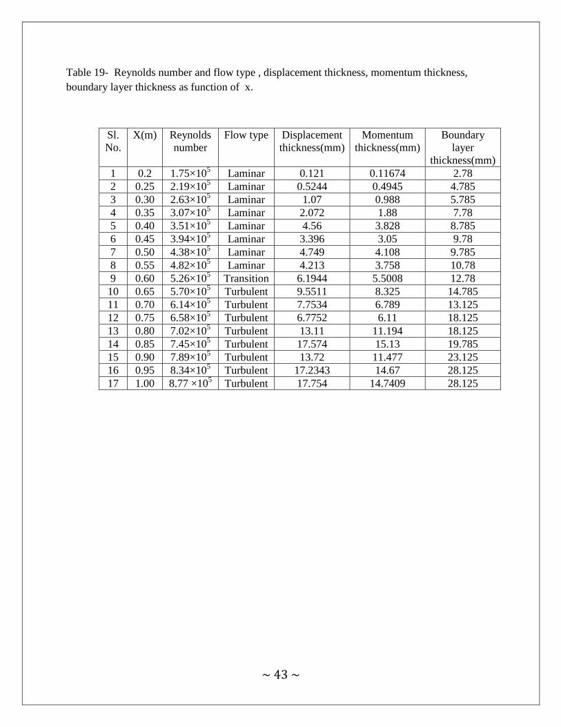
Table 19- Reynolds number and flow type , displacement thickness, momentum thickness,
boundary layer thickness as function of x.
Sl.
No.
X(m) Reynolds
number
Flow type Displacement
thickness(mm)
Momentum
thickness(mm)
Boundary
layer
thickness(mm)
1 0.2 1.75×10⁵ Laminar 0.121 0.11674 2.78
2 0.25 2.19×10⁵ Laminar 0.5244 0.4945 4.785
3 0.30 2.63×10⁵ Laminar 1.07 0.988 5.785
4 0.35 3.07×10⁵ Laminar 2.072 1.88 7.78
5 0.40 3.51×10⁵ Laminar 4.56 3.828 8.785
6 0.45 3.94×10⁵ Laminar 3.396 3.05 9.78
7 0.50 4.38×10⁵ Laminar 4.749 4.108 9.785
8 0.55 4.82×10⁵ Laminar 4.213 3.758 10.78
9 0.60 5.26×10⁵ Transition 6.1944 5.5008 12.78
10 0.65 5.70×10⁵ Turbulent 9.5511 8.325 14.785
11 0.70 6.14×10⁵ Turbulent 7.7534 6.789 13.125
12 0.75 6.58×10⁵ Turbulent 6.7752 6.11 18.125
13 0.80 7.02×10⁵ Turbulent 13.11 11.194 18.125
14 0.85 7.45×10⁵ Turbulent 17.574 15.13 19.785
15 0.90 7.89×10⁵ Turbulent 13.72 11.477 23.125
16 0.95 8.34×10⁵ Turbulent 17.2343 14.67 28.125
17 1.00 8.77 ×10⁵
Turbulent 17.754 14.7409 28.125
~ 44 ~
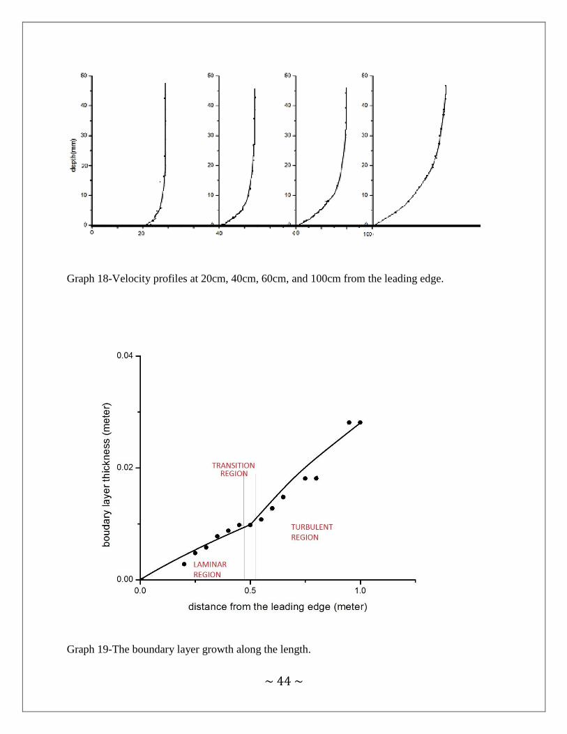
Graph 18-Velocity profiles at 20cm, 40cm, 60cm, and 100cm from the leading edge.
Graph 19-The boundary layer growth along the length.

~ 45 ~
Chapter 6
DISCUSSIONS
AND
RESULTS

~ 46 ~
6 DISCUSSIONS AND RESULTS
1. The Reynolds number shows that the flow transitioned from laminar to turbulent flow
(Re>500,000) after 55 cm from the leading edge of the plate surface. The Reynolds
number is largely a function of speed, viscosity and density of the fluid.
2. The boundary layer thickness is in the range of 2-29 mm, which was expected for the low
speed wind tunnel.
3. The table (19) shows that the thickness increases along the length of the plate.
4. The graph (19) shows the boundary layer thickness v/s length of the plate which give a
clear idea of the boundary layer growth along the plate and also the boundary layer grows
as the length is increased and tends to have great tangent as the velocity increases.
5. The graph(18) shows that the velocity profiles changes along the length of the glass plate.
Initially the velocity profiles have steeper gradient compared to the velocity profiles at
end ones.

~ 47 ~
Chapter 7
CONCLUSIONS

~ 48 ~
7 CONCLUSIONS
Test conducted on a flat plate gave a better understanding of boundary layers and there
parameters. As the wind tunnel is an open tunnel, readings were taken very carefully to
avoid error in the measurement and analysis.
The boundary layer growth which was found out experimentally matched the theoretical
graph.
The velocity profiles gave a clear view of variation which took place along the length of
the glass plate.
The flow transitioned from laminar to turbulent through transition region. The laminar
region and the turbulent region were easily differentiated but it was difficult to get the
transition region from the graph

~ 49 ~
Chapter 8
REFERENCES

~ 50 ~
8 REFERENCES
• Schlichting H. 1979. Boundary-layer theory. 7th ed. New York: McGraw-Hill.
• Boundary Layer Transition effected by surface roughness and Free Stream Turbulence by
S.K . Robert and M .I .Yaras. Journal of Fluid Engineering Volume 124 , Issue 3 May
2005.
• Fluid Mechanics and Fluid Power Engineering by Dr. D.S. Kumar . Katson Publishing
House Delhi . 1999.
• Hydraulic and fluid mechanics including hydraulic machines by DR. P.N.MODI and DR.
S.M.SETH.
• Kay Gemba, California state university, Long Beach, Measurement of boundary layer on
a Flat plate.
• Boundary Layer Transition effected by surface roughness and Free Stream Turbulence b
y S.K. Roberts and M.I.Yaras . Journal of Fluid Engineering Volume 124 , Issue3 Ma y
2005 .