Spreadsheets - University of...
98
Spreadsheets You will learn about some important features of spreadsheets, as well as a few principles for designing and representing information.
Transcript of Spreadsheets - University of...

Spreadsheets
You will learn about some important features of spreadsheets, as well as a few principles for
designing and representing information.
Background
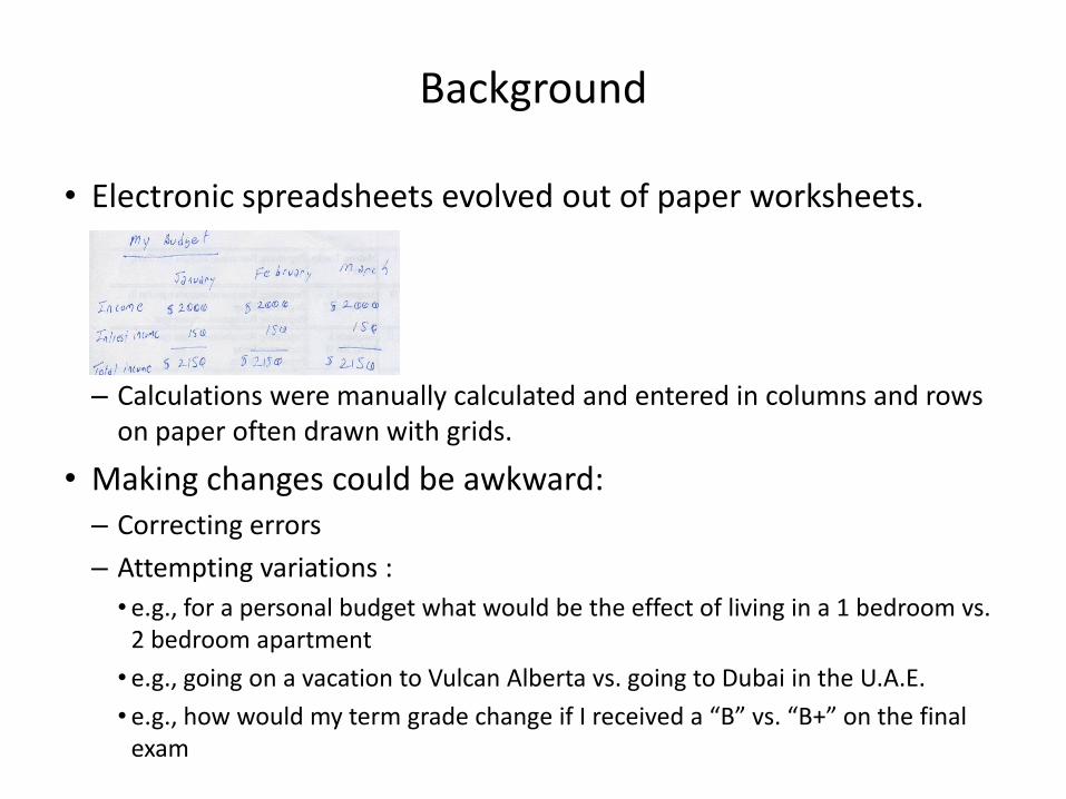
• Electronic spreadsheets evolved out of paper worksheets.
– Calculations were manually calculated and entered in columns and rows
on paper often drawn with grids.
• Making changes could be awkward: – Correcting errors
– Attempting variations :
• e.g., for a personal budget what would be the effect of living in a 1 bedroom vs. 2 bedroom apartment
• e.g., going on a vacation to Vulcan Alberta vs. going to Dubai in the U.A.E.
• e.g., how would my term grade change if I received a “B” vs. “B+” on the final exam

The First Spreadsheet
• Early versions of electronic spreadsheets were primitive but could at least automate calculations.
VISICALC for the Apple II computer: Image from:
http://www.cultofmac.com (last accessed Jan 2015)

Spreadsheets 101
Row numbers
Column headings Coordinates of
current cell
Contents of current cell
Current cell

Worksheets
• Each spreadsheet can consist of multiple worksheets.
Worksheet
Spreadsheet

When To Use Multiple Worksheets
• Rules of thumb: – When there are multiple sheets of related information, each group of
information can be stored in it’s own worksheet.
– Information from one worksheet may be used in another worksheet.
Grades for lecture 01
(worksheet)
Grades for lecture 02
(worksheet)
Grades for lecture 03
(worksheet)
Grades for all sections(spreadsheet)
Budget for dad
(worksheet) Budget for mom
(worksheet)
Budget for sunny-boy
(worksheet)
Family budget (spreadsheet)

When Not To Use Multiple Worksheets
• If the information consists of groups of unrelated information then the information about each group should be stored in a separate spreadsheet/workbook rather than implementing it a spreadsheet with multiple worksheets.
Grades for
mom
(spreadsheet)
Expenses for
the family
business
(spreadsheet)
Daily calorie
intake for dad
(spreadsheet)
The Excel Ribbon
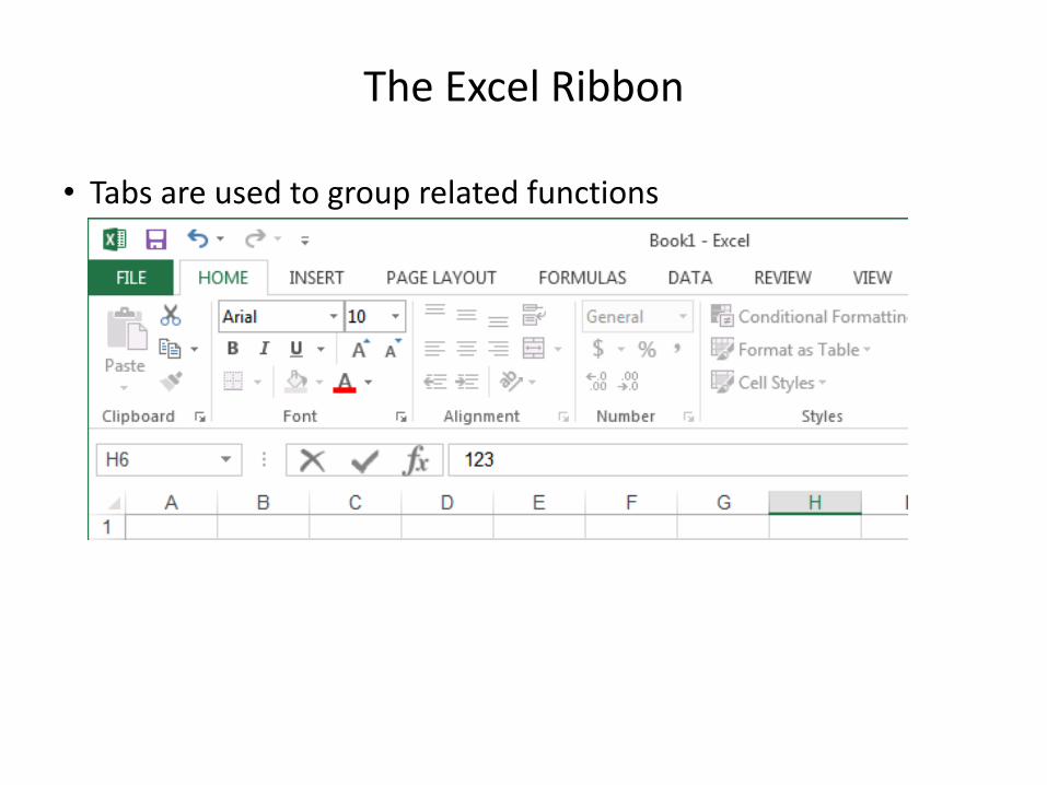
• Tabs are used to group related functions

High Level View Of Each Tab
• File: – Functions associated with documents (creating, opening, saving, printing
etc.)
• Home (default) **: – Many of the most commonly used functions (such as formatting fonts,
cells and numerical data)
• Insert: – Tables, illustrations, apps, charts, graphs, text, and symbols
• Page layout: – Page setup (many similar to print options)
• Formulas *: – Location and groupings of the pre-created built-in mathematical formulas

High Level View Of Each Tab (2)
• Data: – Arranging, organizing existing data (e.g., sort)
• Review: – Proofing, Language, Comments, and Changes
• View (different views of the same data): – Workbook Views, Show, Zoom, Window, and Macros
Customizing The Ribbon
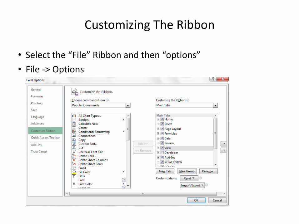
• Select the “File” Ribbon and then “options”
• File -> Options

Constants (Data) Vs. Calculations
• In the cell calculations are signified with a leading ‘=‘ (equals sign)
• Example:
4.2 3.3 =(A2*0.4)+(B2*0.6)
Designing Spreadsheets: Rules Of Thumb
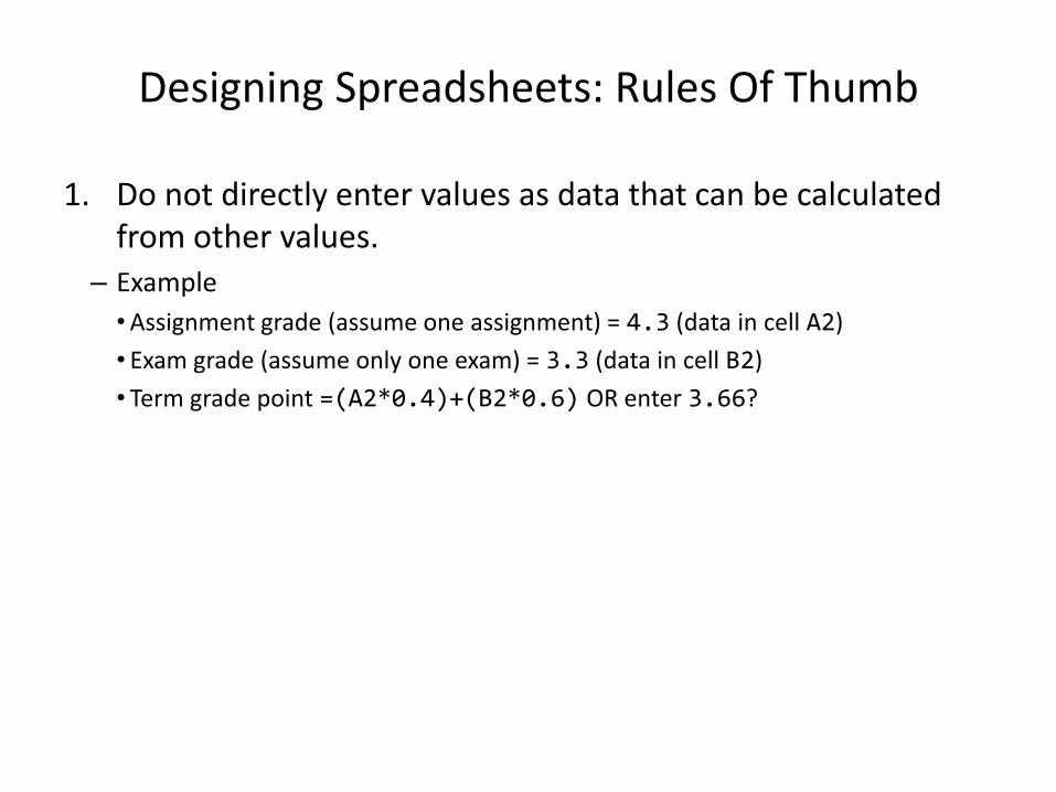
1. Do not directly enter values as data that can be calculated from other values.
– Example
• Assignment grade (assume one assignment) = 4.3 (data in cell A2)
• Exam grade (assume only one exam) = 3.3 (data in cell B2)
• Term grade point =(A2*0.4)+(B2*0.6) OR enter 3.66?
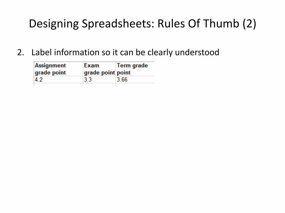
Designing Spreadsheets: Rules Of Thumb (2)
2. Label information so it can be clearly understood
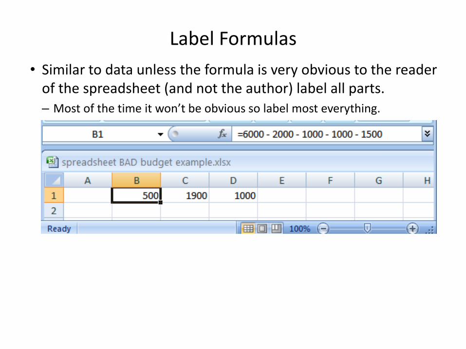
Label Formulas
• Similar to data unless the formula is very obvious to the reader of the spreadsheet (and not the author) label all parts. – Most of the time it won’t be obvious so label most everything.

Previous Example: Explicitly Labeled Formulas
• Whenever possible label the different parts of a calculation to make easier for the reader to interpret and understand how your calculations work.

Designing Spreadsheets: Rules Of Thumb (3)
3. Never enter the same information more than once – Advantages: reduces size and complexity of the sheet, making changes
can be easier.
– Seems obvious? Not always
– Example: What if the previous spreadsheet were used to calculate the grades for a class full of students?
– Some would create the sheet this way:
– spreadsheet example name: example1_grades.xlsx
=(B2*0.4)+(C2*0.6)
=(B2*0.4)+(C2*0.6)
Etc.
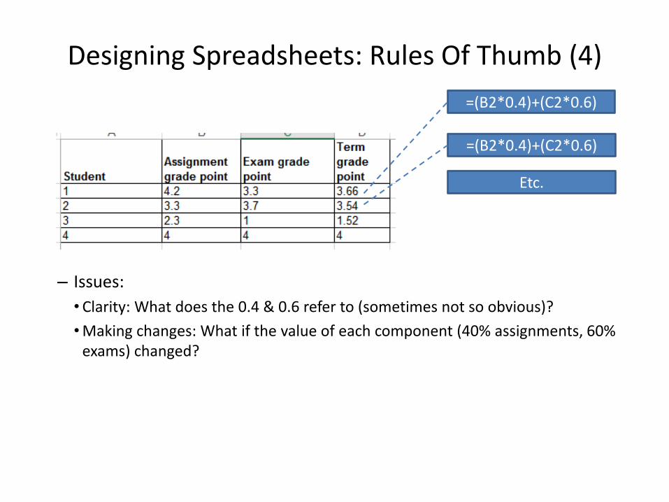
Designing Spreadsheets: Rules Of Thumb (4)
– Issues:
• Clarity: What does the 0.4 & 0.6 refer to (sometimes not so obvious)?
• Making changes: What if the value of each component (40% assignments, 60% exams) changed?
=(B2*0.4)+(C2*0.6)
=(B2*0.4)+(C2*0.6)
Etc.

Lookup Tables
• As the name implies it contains information that needs to be referred to (“looked up”) in a part of the spreadsheet.
• Can be used to address some of the issues related to the previous example: – Clarity
– Entering the same data multiple times =(B2*G2)+(C2*G3)
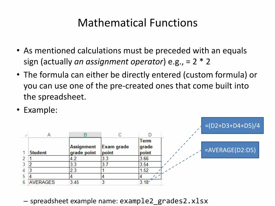
Mathematical Functions
• As mentioned calculations must be preceded with an equals sign (actually an assignment operator) e.g., = 2 * 2
• The formula can either be directly entered (custom formula) or you can use one of the pre-created ones that come built into the spreadsheet.
• Example:
– spreadsheet example name: example2_grades2.xlsx
=(D2+D3+D4+D5)/4
=AVERAGE(D2:D5)
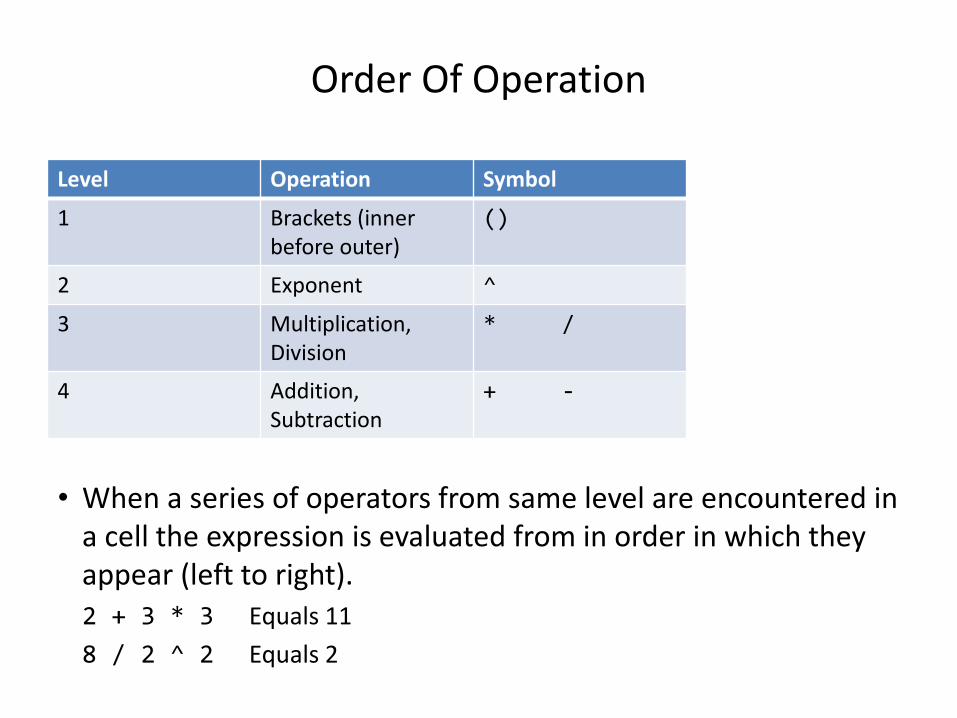
• When a series of operators from same level are encountered in a cell the expression is evaluated from in order in which they appear (left to right). 2 + 3 * 3 Equals 11
8 / 2 ^ 2 Equals 2
Order Of Operation
Level Operation Symbol
1 Brackets (inner before outer)
()
2 Exponent ^
3 Multiplication, Division
* /
4 Addition, Subtraction
+ -
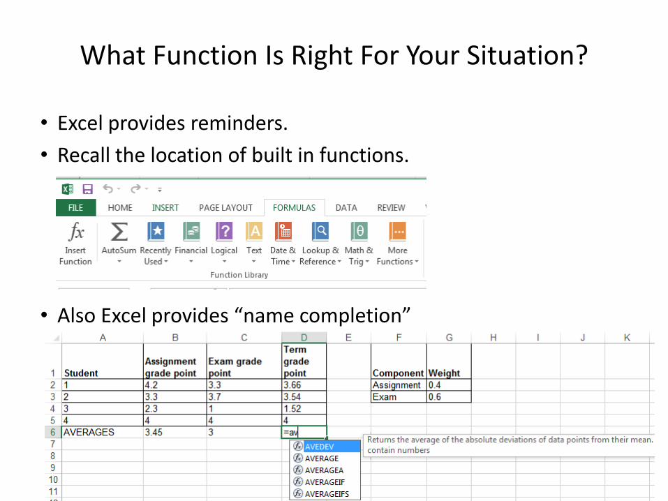
What Function Is Right For Your Situation?
• Excel provides reminders.
• Recall the location of built in functions.
• Also Excel provides “name completion”

Built-In Excel Functions
• They will be covered in greater detail in tutorial – “Lookup functions” excepted (because they relate to a concept that will
be covered in lecture “if-branching”)
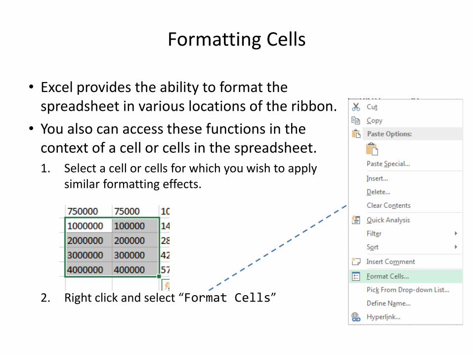
Formatting Cells
• Excel provides the ability to format the spreadsheet in various locations of the ribbon.
• You also can access these functions in the context of a cell or cells in the spreadsheet. 1. Select a cell or cells for which you wish to apply
similar formatting effects.
2. Right click and select “Format Cells”

Formatting Cells (2)
• General: no special format
• Number: • number of
decimal places. • Separator (every
3 digits)

Formatting Cells (3)
• General: no special format • Number:
• Separator (3 digits) • Several options for displaying
negative numbers • Currency:
• Currency sign • Several options for displaying
negative numbers • Columns aligns decimal points
• Accounting: • Similar to currency but no special
options for displaying negative values
• Date, Time: • Both allow display in different
formats • Percentage: % • Fraction: /
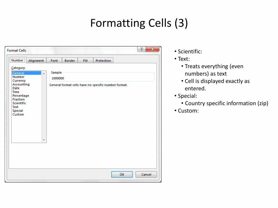
Formatting Cells (3)
• Scientific: • Text:
• Treats everything (even numbers) as text
• Cell is displayed exactly as entered.
• Special: • Country specific information (zip)
• Custom:

Autofill
• Allows for a series to be extended – E.g., The series “1, 2, 3” (can be extended to include “…4, 5, 6”)
• Steps: 1. Highlight the cells containing the series to extend (selecting one cell just
repeats the contents of that one cell).
2. Move the mouse pointer to the ‘handle’ at the bottom right

Autofill (2)
3. Drag the mouse as far down as you wish the series to be extended to.

‘If-Else’ (Branching)
• Returns one value if a condition has been met. – “If condition met”
• Can return another value if the condition hasn’t been met. – “Else if the condition not met”
• Boolean (logic): either true or false that the condition was met
Grade >= 50%
“Passed”
True
“Failed”
False

Applying Branches: Grade Example
• (Assume that a grade point of 3.0 or greater is required as the minimum cut-off for ‘honors’ for a course).
• In column ‘E’ the sheet will display “Honors student” if term grade point is 3.0 or greater “Not honors” otherwise. – spreadsheet example name: example3_if_grades.xlsx
=IF(D2>=3,"Honors student","Not honors")
Condition Condition true Condition false “else”
Format: If-Else
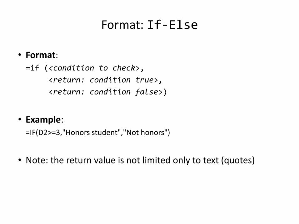
• Format:
=if (<condition to check>,
<return: condition true>,
<return: condition false>)
• Example: =IF(D2>=3,"Honors student","Not honors")
• Note: the return value is not limited only to text (quotes)

Comparators
Math Excel Meaning
< < Less than
> > Greater than
= = Equal to
≤ <= Less than, equal to
≥ >= Greater than, equal to
≠ <> Not equal to
If: Specifying Only The True Case
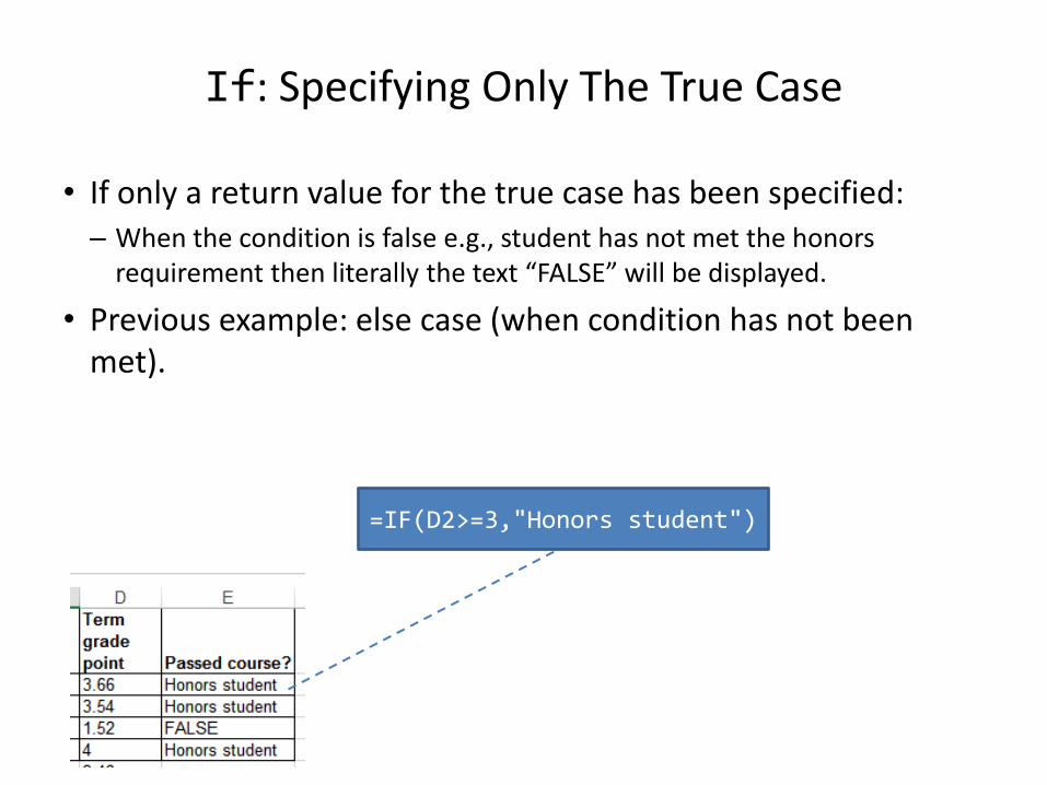
• If only a return value for the true case has been specified: – When the condition is false e.g., student has not met the honors
requirement then literally the text “FALSE” will be displayed.
• Previous example: else case (when condition has not been met).
=IF(D2>=3,"Honors student")

If: Specifying Only The True Case (2)
• Consequently: – Even if a specific return value is desired only for the ‘if condition case’
(true that the condition has been met)
– Something, even an empty message, should be specified for the ‘else case’ (false that the condition has been met).
• Previous example: amended
– spreadsheet example name: example3A_if_only_grades.xlsx
=IF(D2>=3,"Honors student","")

Nested Conditions
• Applies when different conditions must be checked
• Example: – Display “Perfect” if grade point is 4.0 or greater
– Display “Excellent” if grade point is 3.0 or greater but less than 4.0
– Display “Adequate” if grade point is 2.0 or greater but less than 3.0
– Display “Pass” if grade point is 1.0 or greater but less than 2.0
– Otherwise display “Fail”
– spreadsheet example name: example4_nested_if_grades.xlsx

Previous Grade Example: Specifying Conditions
GPA >= 4.0? “Perfect” True
“Fail”
False
GPA >= 3.0? “Excellent” True
False
GPA >= 2.0? “Adequate” True
False
GPA >= 1.0? “Pass” True
False
Nesting • Later conditions are
described as being ‘nested’ within early conditions
• The GPA cases for 3.0, 2.0, 1.0 are described as being ‘nested’ within the 4.0 case (only checked if the previous case proves to be false)
Previous Example: Initial Cases
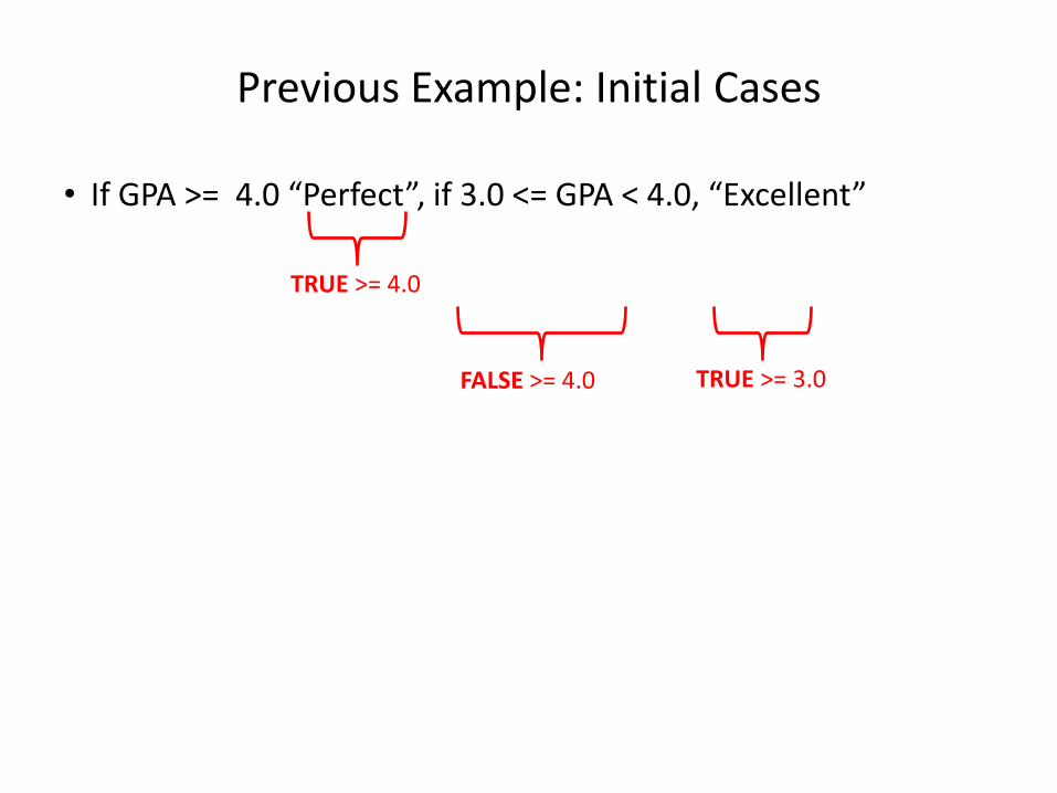
• If GPA >= 4.0 “Perfect”, if 3.0 <= GPA < 4.0, “Excellent”
TRUE >= 4.0
FALSE >= 4.0 TRUE >= 3.0

Previous Example: Nested Solution
=IF(D2>=4,"Perfect", IF(D2>=3,"Excellent", IF(D2>=2,"Adequate", IF(D2>=1,"Pass", "Fail"))))
=IF(D2>=4,"Perfect",IF(D2>=3,"Excellent",IF(D2>=2,"Adequate",IF(D2>=1,"Pass","Fail"))))
T
F
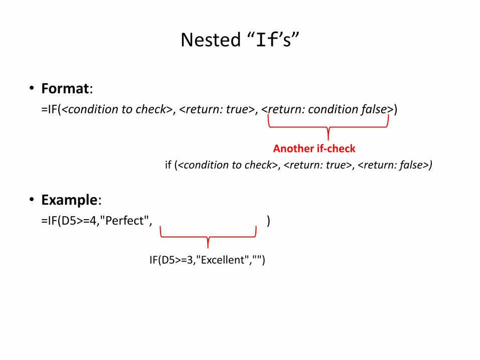
Nested “If’s”
• Format: =IF(<condition to check>, <return: true>, <return: condition false>)
• Example: =IF(D5>=4,"Perfect", )
if (<condition to check>, <return: true>, <return: false>)
Another if-check
IF(D5>=3,"Excellent","")
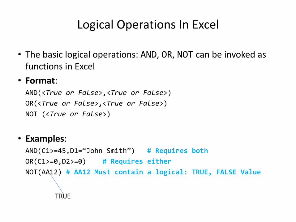
Logical Operations In Excel
• The basic logical operations: AND, OR, NOT can be invoked as functions in Excel
• Format: AND(<True or False>,<True or False>)
OR(<True or False>,<True or False>)
NOT (<True or False>)
• Examples: AND(C1>=45,D1=“John Smith”) # Requires both
OR(C1>=0,D2>=0) # Requires either
NOT(AA12) # AA12 Must contain a logical: TRUE, FALSE Value
TRUE

Logic And IF’s: Example
• The honor roll for each semester requires that grade point is 3.7 or greater and a full load of at least 5 courses must be taken.
• Signify when a student has met the honor roll requirements with an “H”, blank cell otherwise.
– Spreadsheet example name: example5_if_logic.xlsx
=IF(AND(B5>=3.7,C5>=5),"H","")

Conditional Formatting
• A very practical example of how conditional branching “if’s” can be applied.
• Use of conditional formatting will be covered in tutorial.

Lookup Tables
• Can be instead of many nested IF’s. – Easier to enter, update, understand.
• Requirements of previous example: 0 <= GPA < 1: Fail
1 <= GPA < 2 : Pass
2 <= GPA < 3 : Adequate
3 <= GPA < 4 : Excellent
GPA >= 4 : Perfect
• Previous solution: =IF(D2>=4,"Perfect",IF(D2>=3,"Excellent",IF(D2>=2,"Adequate",IF(D2>=1,"Pass","Fail"))))

VLOOKUP
• A function that can be used to lookup values from a table. – Another function (“LOOKUP”) will be covered in tutorial
• Format: VLOOKUP(<Lookup value>, *
<Lookup table Start : End>, *
<Lookup table Return value>, *
<Exact match required?>)
– A star * indicates a required value.
• Example: =VLOOKUP(D2, D11:E15, 2)
Cell: Contains value to find in table e.g., a grade point
Lookup table: Start : End cell coordinates
Lookup table: Column value to return (1 = first col. ‘D’, 2 = second col. ‘E’)
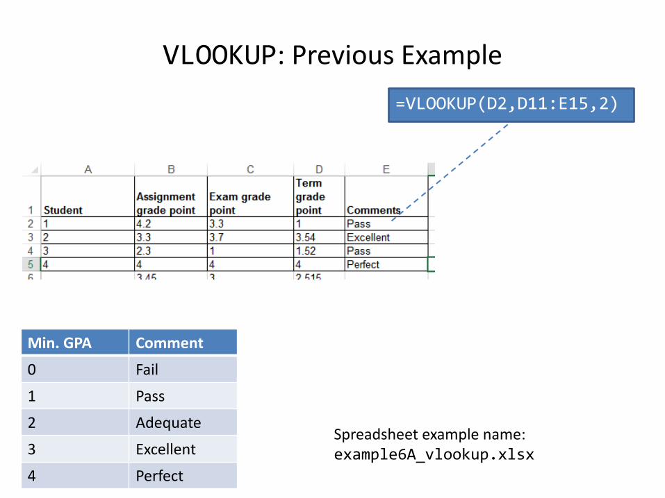
VLOOKUP: Previous Example
Min. GPA Comment
0 Fail
1 Pass
2 Adequate
3 Excellent
4 Perfect
=VLOOKUP(D2,D11:E15,2)
Spreadsheet example name: example6A_vlookup.xlsx
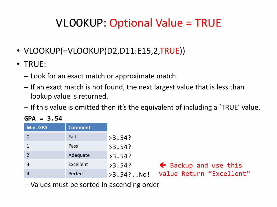
VLOOKUP: Optional Value = TRUE
• VLOOKUP(=VLOOKUP(D2,D11:E15,2,TRUE))
• TRUE: – Look for an exact match or approximate match.
– If an exact match is not found, the next largest value that is less than lookup value is returned.
– If this value is omitted then it’s the equivalent of including a ‘TRUE’ value.
– Values must be sorted in ascending order
Min. GPA Comment
0 Fail
1 Pass
2 Adequate
3 Excellent
4 Perfect
GPA = 3.54
>3.54?
>3.54?
>3.54?
>3.54?
>3.54?..No!
Backup and use this value Return “Excellent”

VLOOKUP: Optional Value = FALSE
• VLOOKUP(=VLOOKUP(D2,D11:E15,2,FALSE))
• FALSE: – Looks only for an exact match
– If a match is found then the value at the specified location is returned.
– Else if no match is found the an error message is displayed.
– Table values do not have to be sorted.
Min. GPA Comment
0 Fail
1 Pass
2 Adequate
3 Excellent
4 Perfect

Additional Resources: VLOOKUP
•For more information about VLOOKUP and other Excel functions use the help lookup “?”
•Specific help for VLOOKUP: •http://office.microsoft.com/en-ca/excel-help/vlookup-
HP005209335.aspx
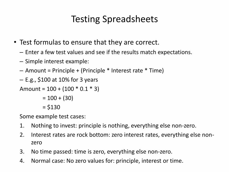
Testing Spreadsheets
• Test formulas to ensure that they are correct. – Enter a few test values and see if the results match expectations.
– Simple interest example:
– Amount = Principle + (Principle * Interest rate * Time)
– E.g., $100 at 10% for 3 years
Amount = 100 + (100 * 0.1 * 3)
= 100 + (30)
= $130
Some example test cases:
1. Nothing to invest: principle is nothing, everything else non-zero.
2. Interest rates are rock bottom: zero interest rates, everything else non-zero
3. No time passed: time is zero, everything else non-zero.
4. Normal case: No zero values for: principle, interest or time.

Example Testing A Formula
<- All non-zero
<- No principle
<- No interest <- No time elapsed

Testing Ranges
• The following are the minimum test cases
• Provide test values for each range – In this example try grade points of 0, 1, 2, 3, 4
• Also for at least one of the ranges test the boundaries (just above and below) – Example: testing the boundary for 1 / “Pass”
– Slightly above a boundary value e.g., 0.9 should return “Fail”
– Slightly above a boundary value e.g., 1.1 should return “Pass”
Min. GPA Comment
0 Fail
1 Pass
2 Adequate
3 Excellent
4 Perfect
Methods Of Referring To Cells
• Absolute
• Relative
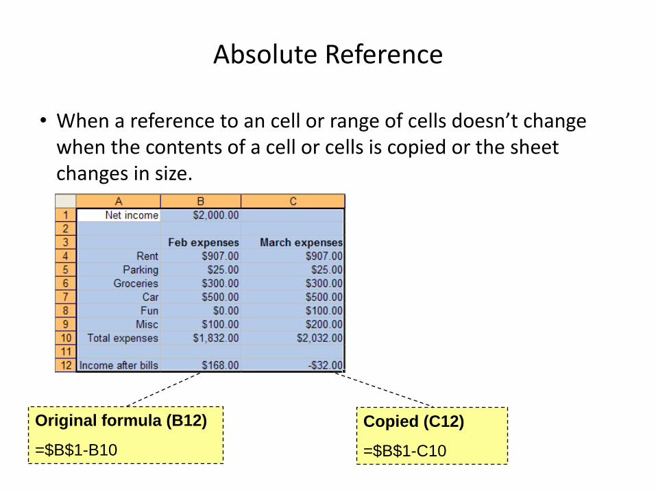
Absolute Reference
• When a reference to an cell or range of cells doesn’t change when the contents of a cell or cells is copied or the sheet changes in size.
Original formula (B12)
=$B$1-B10
Copied (C12)
=$B$1-C10
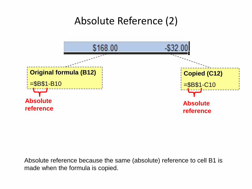
Absolute Reference (2)
Original formula (B12)
=$B$1-B10
Copied (C12)
=$B$1-C10
Absolute
reference Absolute
reference
Absolute reference because the same (absolute) reference to cell B1 is
made when the formula is copied.
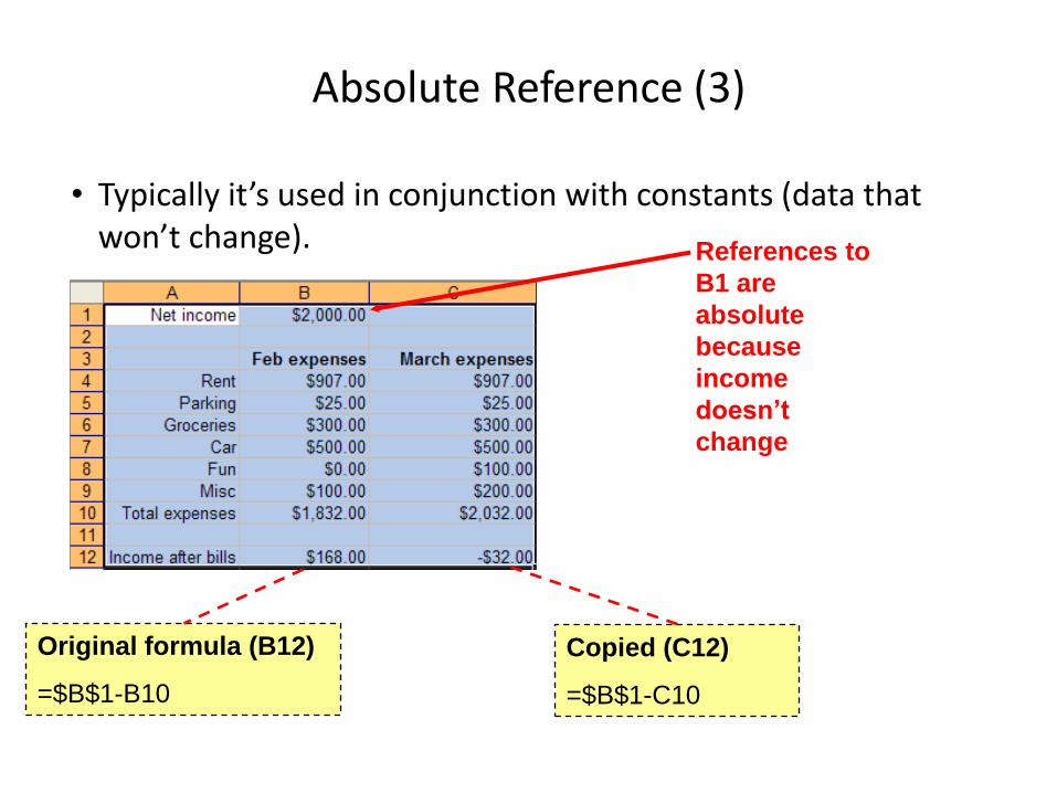
Absolute Reference (3)
• Typically it’s used in conjunction with constants (data that won’t change).
Original formula (B12)
=$B$1-B10
Copied (C12)
=$B$1-C10
References to
B1 are
absolute
because
income
doesn’t
change
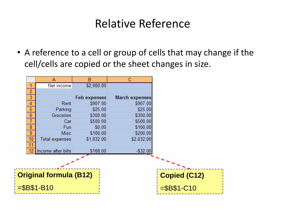
Relative Reference
• A reference to a cell or group of cells that may change if the cell/cells are copied or the sheet changes in size.
Original formula (B12)
=$B$1-B10
Copied (C12)
=$B$1-C10
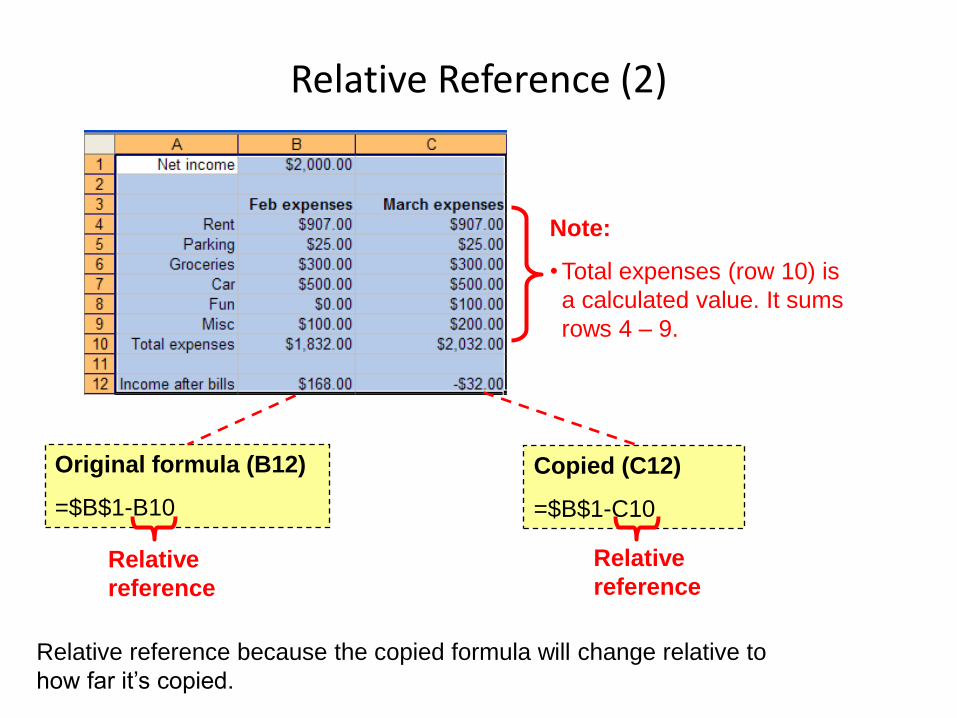
Relative Reference (2)
Original formula (B12)
=$B$1-B10
Copied (C12)
=$B$1-C10
Note:
• Total expenses (row 10) is
a calculated value. It sums
rows 4 – 9.
Relative
reference
Relative
reference
Relative reference because the copied formula will change relative to
how far it’s copied.

Relative Reference (3)
• Typically it’s used with variable data (that may change over time or in different parts of the sheet).
Original formula (B12)
=$B$1-B10
Copied (C12)
=$B$1-C10
Total expenses may
change from month-
to-month so
references will likely
be relative.
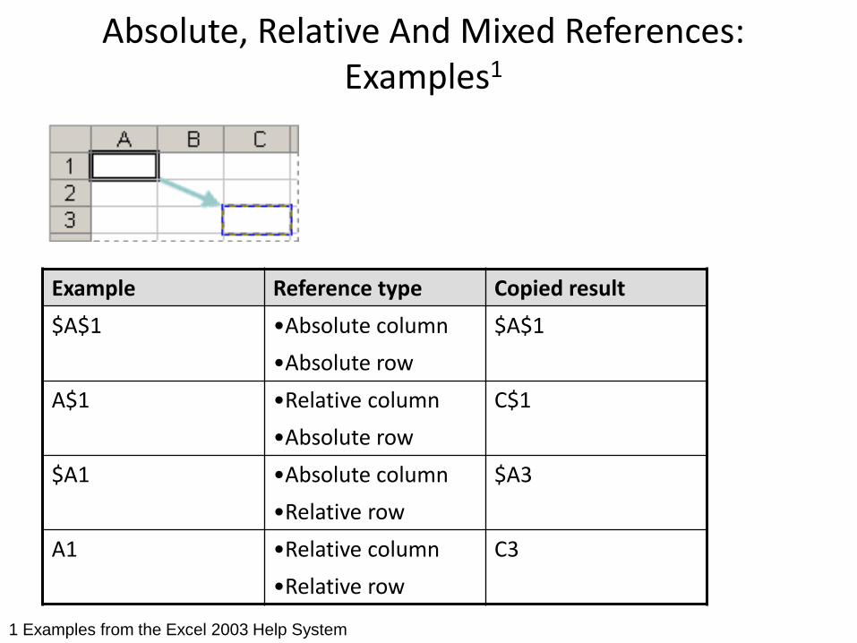
Absolute, Relative And Mixed References: Examples1
Example Reference type Copied result
$A$1 •Absolute column
•Absolute row
$A$1
A$1 •Relative column
•Absolute row
C$1
$A1 •Absolute column
•Relative row
$A3
A1 •Relative column
•Relative row
C3
1 Examples from the Excel 2003 Help System

Absolute & Relative References: Extra
• With the previous examples, which part of each formula should be an absolute reference and which part should be a relative reference.
=VLOOKUP(D2,D11:E15,2)
• Don’t look at the solution until you have tried working it out yourself!
• Spreadsheet solution name: example6B_vlookup_absolute_relative_addressing

Graphic Design And Spreadsheets
• Using color
• C.R.A.P.
• Fonts and font effects
• Text vs. graphs and charts
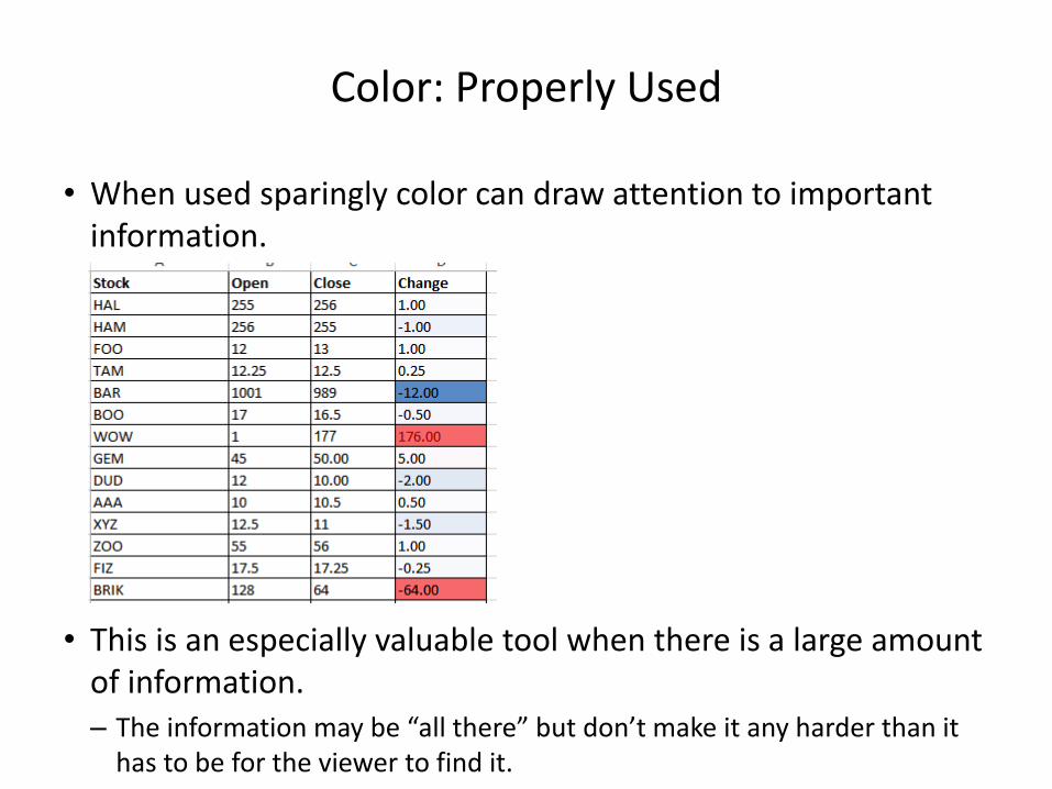
Color: Properly Used
• When used sparingly color can draw attention to important information.
• This is an especially valuable tool when there is a large amount of information. – The information may be “all there” but don’t make it any harder than it
has to be for the viewer to find it.

Color Misused
• The overuse of color: – Reduces it’s ability to make information stand out.
– Makes it harder to understand what information is mapped to a particular color.

Rule Of Thumb For Color: Make It Subtle
• We have all seen the use of ‘loud’ and clashing colors that can make text very hard to read.
• Balance the use of color between noticeability and subtlety – Make it as subtle as possible while still conveying the necessary
information using color
Ingredients Sugar, lactose, fructose, corn syrup, glucose…lots of carbohydrates
JT: I’ve actually seem green-red color combinations on listings of ingredients
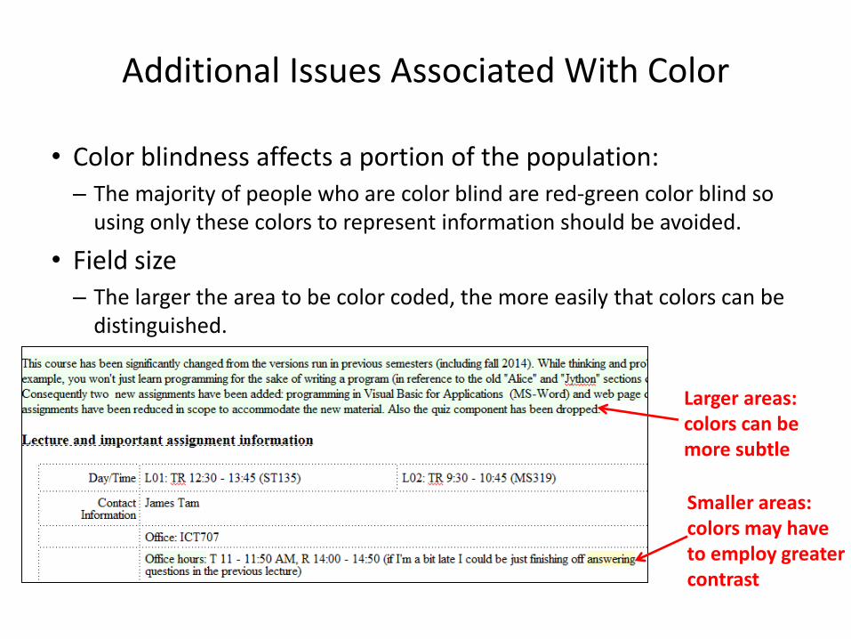
Additional Issues Associated With Color
• Color blindness affects a portion of the population: – The majority of people who are color blind are red-green color blind so
using only these colors to represent information should be avoided.
• Field size – The larger the area to be color coded, the more easily that colors can be
distinguished.
Larger areas: colors can be more subtle
Smaller areas: colors may have to employ greater contrast

Additional Issues Associated With Color (2)
– When objects are small (text or small graphics) and color is used to distinguish information use highly saturated colors.
• Conventions – “Commonly accepted” conventions can vary widely by culture and their
use should be carefully considered
This is
important
information!
This is
important
information!

Color And Cultural Associations
Egypt China Japan India France
Red • Death •Happiness • Anger,
Danger
• Life,
creativity
• Aristocracy,
Freedom,
Peace
Blue • Virtue, Faith,
Truth
• Heavens,
Clouds
•Villainy • Freedom,
peace
Green • Fertility,
Strength
• Ming
Dynasty,
Heavens,
Clouds
• Future,
Youth,
Energy
• Prosperity,
Fertility
•Criminality
Yellow • Happiness,
Prosperity
• Birth,
Wealth,
Power
• Grace,
Nobility
•Success •Temporary
White •Joy • Death,
Purity
•Death • Death,
Purity
•Neutrality
From “How Fluent is Your Interface? Designing for International Users” Proceedings of the INTERCHI’93. Russo P.
and Boor S.

Fonts And Font Effects
• Example fonts: – Ariel
– Calibri
– Helvetica
– Times New Roman
• Font effects: – Italics
– Bold
– Underline
– Normal
• Font sizes
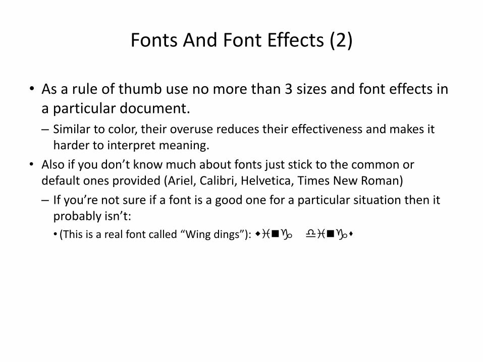
Fonts And Font Effects (2)
• As a rule of thumb use no more than 3 sizes and font effects in a particular document. – Similar to color, their overuse reduces their effectiveness and makes it
harder to interpret meaning.
• Also if you don’t know much about fonts just stick to the common or default ones provided (Ariel, Calibri, Helvetica, Times New Roman)
– If you’re not sure if a font is a good one for a particular situation then it probably isn’t:
• (This is a real font called “Wing dings”): wing dings

C.R.A.P.1
• Simple design principles that can be applied in a variety of situations
• Contrast
• Repetition
• Alignment
• Proximity
1 From “The non-designers type book” by Robin Williams (Peach Pit express)
Contrast & Repetition
• Contrast: – Make different things look significantly different
• Repetition (Consistency): – Repeat conventions throughout the interface to tie elements together

Example: No Contrast

Example: Weak Contrast

Example: Headings Stand Out
• Good contrast: – If contrast is not (or weakly) employed for a small set of data it may not
be a large issue.
– But for larger data sets (“real data”) it may make it more work than is necessary.
• Repetition: – Same fonts, font sizes and font effects used in the headings vs. the data.
– Makes it easier to see and understand the structure

Alignment
• It can be used to structure a document (represents hierarchical relationships).
Alignment And Repetition
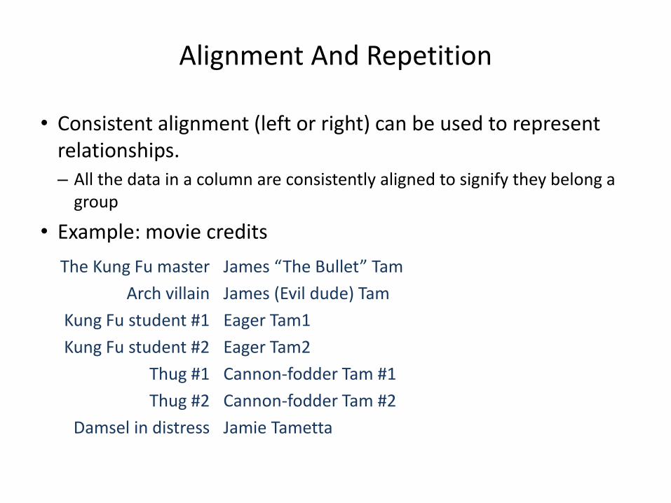
• Consistent alignment (left or right) can be used to represent relationships. – All the data in a column are consistently aligned to signify they belong a
group
• Example: movie credits
The Kung Fu master
Arch villain
Kung Fu student #1
Kung Fu student #2
Thug #1
Thug #2
Damsel in distress
James “The Bullet” Tam
James (Evil dude) Tam
Eager Tam1
Eager Tam2
Cannon-fodder Tam #1
Cannon-fodder Tam #2
Jamie Tametta

Centre Alignment
• Sparing use can be used to provide contrast e.g., slide titles vs. content.
• Because they remove a common method for structuring a document it can make reading text more difficult.

Center Alignment
• Again: while sparing use of center alignment can be used to provide contrast it should NEVER be used as the default in documents such as spreadsheets.

Proximity
• Related items are in close proximity
• Unrelated items are separated

Text Or Graphics?
• Text?
• A graph or chart? – What type to use? (Pie, bar, line etc.)

The Benefits Of Using Text
• Text is the best representation to use when accuracy is paramount.
• Example term grades for individual students.
Student ID Percentage 111 95 222 88 333 100 444 66 555 86 666 79
0
20
40
60
80
100
120
0 200 400 600 800
Percentages
PercentageVs.
Benefits Of Graphics
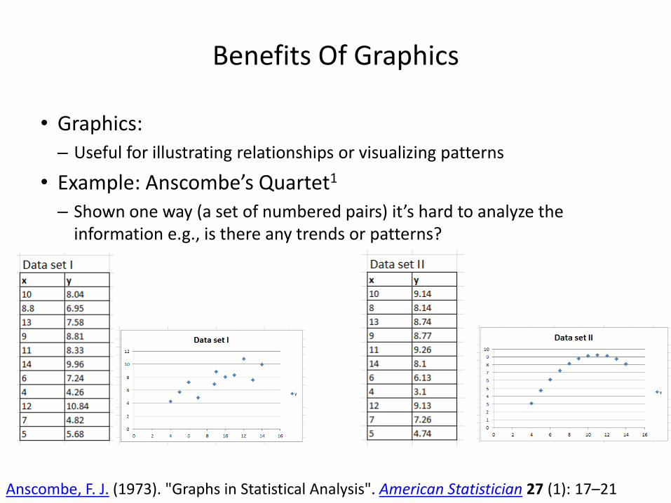
• Graphics: – Useful for illustrating relationships or visualizing patterns
• Example: Anscombe’s Quartet1
– Shown one way (a set of numbered pairs) it’s hard to analyze the information e.g., is there any trends or patterns?
Anscombe, F. J. (1973). "Graphs in Statistical Analysis". American Statistician 27 (1): 17–21
Benefits Of Graphics (2)
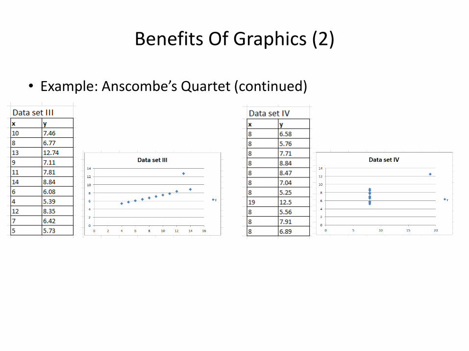
• Example: Anscombe’s Quartet (continued)

Benefits Of Graphics (3)
• Graphical representations can make a powerful impression!
Letter
No.
occurrences
F 0
D 1
D+ 1
C- 2
C 8
C+ 12
B- 17
B 25
B+ 33
A- 45
A 30
A+ 10
0
5
10
15
20
25
30
35
40
45
50
F D D+ C- C C+ B- B B+ A- A A+
No. occurrences
No. occurrences
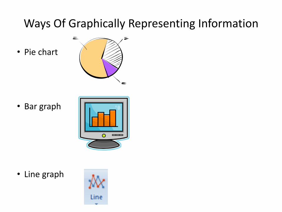
Ways Of Graphically Representing Information
• Pie chart
• Bar graph
• Line graph

Pie Charts
• Good for showing proportions, how much of the whole does each item contribute.
• It’s poor for showing exact numeric values.
Grade distribution
FDCB
No. of students receiving each grade
F
D
C
B

Bar And Line Graphs
•For showing trends
•Comparing functions
Productivity for 2003
0
10
20
30
40
50
60
Jan Feb Mar Apr May Jun Jul Aug Sep Oct Nov Dec
2003
Wo
rk o
utu
pu
t
Work output
0
5
10
15
20
25
30
35
40
F D D+ C- C C+ B- B B+ A- A A+ W
No. occurances
Letter
No. occurances

Rules Of Thumb For Graphs
1. The X axis is used to plot known data (e.g., letter grades), while the Y axis is used to plot the unknown data (e.g., the number of students who received particular letter grades).
0
5
10
15
20
25
30
35
40
F D D+ C- C C+ B- B B+ A- A A+ W
No. occurances
Letter
No. occurances
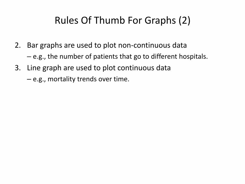
Rules Of Thumb For Graphs (2)
2. Bar graphs are used to plot non-continuous data
– e.g., the number of patients that go to different hospitals.
3. Line graph are used to plot continuous data
– e.g., mortality trends over time.

Excel And Other Spreadsheets
• Excel: – The most commonly used format (along with other MS-Office products).
– Other office software claiming compatibility with MS-Office documents aren’t always 100% compatible.
– Familiar interface
• Google spreadsheet: – Part of the “Google docs” suite of programs.
– Why use it: It’s free and doesn’t require an install on a particular computer operating system.
– Normally documents are saved on the Google servers (convenient but balance that out vs. potential security concerns – private data stored on another company’s servers).
– Simple interface but fewer features than office.

Excel And Other Spreadsheets
• Open Office: – Acquired by Sun Microsystems and eventually provided in an open source
form (access license is free)
– Documents are stored in its own format but could read other formats (including MS-Office).
– Available for many operating systems: Linux, Windows and later for it was also available for Solaris and Apple’s OS X.
– Now part of the Apache Software Foundation
– Free
– Not as widely used as MS-Office and not 100% compatible
– Interface may be foreign to MS-Office users
– https://www.openoffice.org/
Sources: Other Spreadsheet
• When looking online for comparisons beware of biased reviews e.g., “The Google spreadsheet must be good because everything that comes out of that company is just great!” – Paraphrased from an actual ‘review’
• Fairly reasonable sources – http://www.cogniview.com/blog/spreadsheet-battle-excel-vs-google/
– http://www.usatoday.com/story/tech/2013/08/31/review-google-apple-decent-contenders-to-office/2723315/
– http://www.techradar.com/reviews/pc-mac/software/business-and-finance-software/apache-openoffice-4-0-1171091/review
After This Section You Should Now Know
• The benefit of electronic over paper spreadsheets
• Spreadsheets 101: The basic layout and components of a spreadsheet
• What is a worksheet – When to use multiple spreadsheets vs. multiple worksheets
• How Excel groups functions according to tabs on the ribbon – What are the most commonly used tabs and what some of the functions
available on those tabs
• What is the difference between constants (data) and calculations (formulas) – How is a formula differentiated from data

After This Section You Should Now Know (2)
• The three rules of thumb for designing spreadsheets 1. Don’t make something data if it can be derived
2. Label everything
3. Don’t duplicate data
• Lookup tables – How to create a use a lookup table
• Formulas: – Directly entering custom formulas
– Using built-in pre-created formulas
– What is the order of operation for common operators
• How to format cells using the “format cell” option – What is the effect of different numeric formatting options
• How to use the auto fill operation
After This Section You Should Now Know (3)
• How to use ‘if-else’ for branches that return different values – The different ways of expressing logical comparators
– How to write or evaluate nested ‘if’s’
• Logical operations in Excel: AND, OR, NOT – How to write or evaluate logical operations
– How to apply the logical operations in conjunction with the ‘if-else’
• How to use the VLOOKUP function
• How to come up with set of reasonable test cases for a spreadsheet – Formulas and ranges
• What is the difference between an absolute vs. relative cell reference and when to use each one

After This Section You Should Now Know (4)
• Rules for using and not misusing color
• Issues associated with color: color blindness, field size, conventions for color
• Rules of thumb for using fonts and font effects
• C.R.A.P. – What does each part mean
– How it can be used for effective graphic design
• When to use text vs. graphics
• When to use a pie chart vs. bar graph vs. line graph

Copyright Notification
• “Unless otherwise indicated, all images in this presentation are used with permission from Microsoft.”
• Images of spreadsheets (save VisiCalc) are curtesy of James Tam
slide 98