Photometric Techniques IPreliminary reductions and calibrations

Sergio Ortolani

Dipartimento di AstronomiaUniversita’ di Padova,Italy

.

CCD “optical” PHOTOMETRY vs.

Phtoelectric photometryIR array photometry

STELLAR PHOTOMETRYSURPHACE PHOTOMETRY

STELLAR CCD PHOTOMETRYTargets: star clusters, field stars

in the MW and in external galaxies.Peculiar isolated stars (SNs, Nova

stars, NS, GRBs, X-Ray sources…).Variable stars (stars with planets).Typical goal 1-5% accuracy in the

standard U, B, V, R, I (Gunn z)

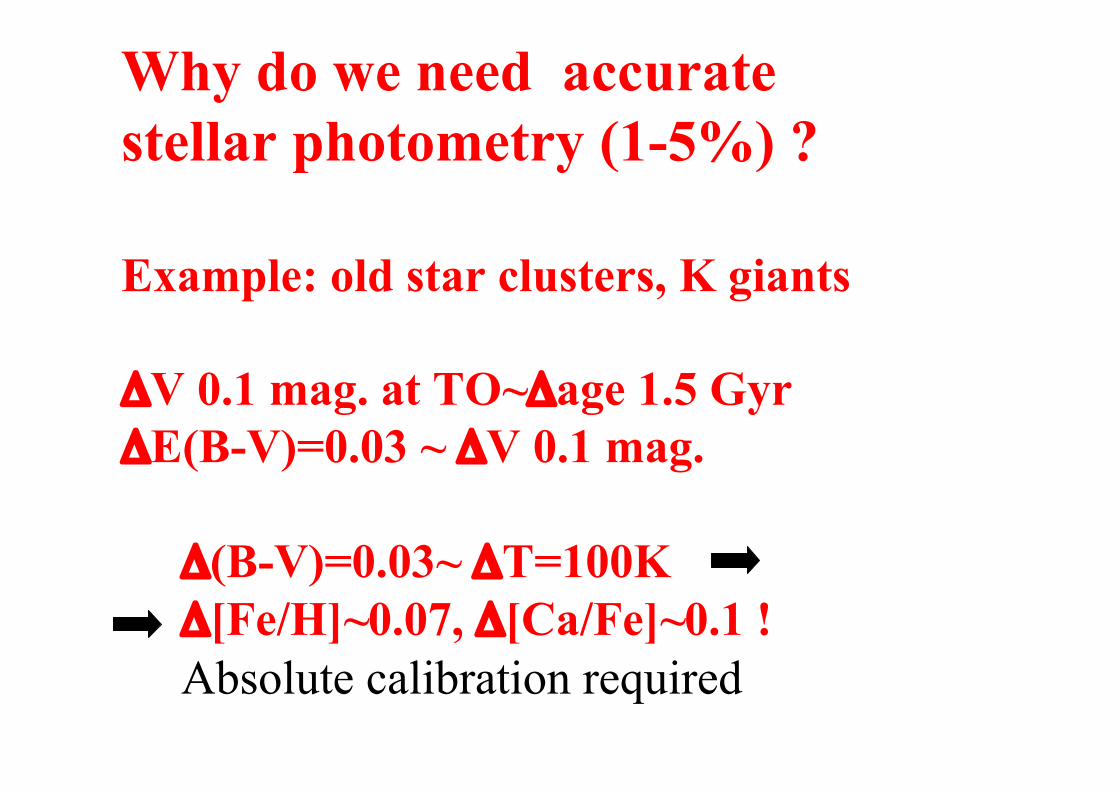
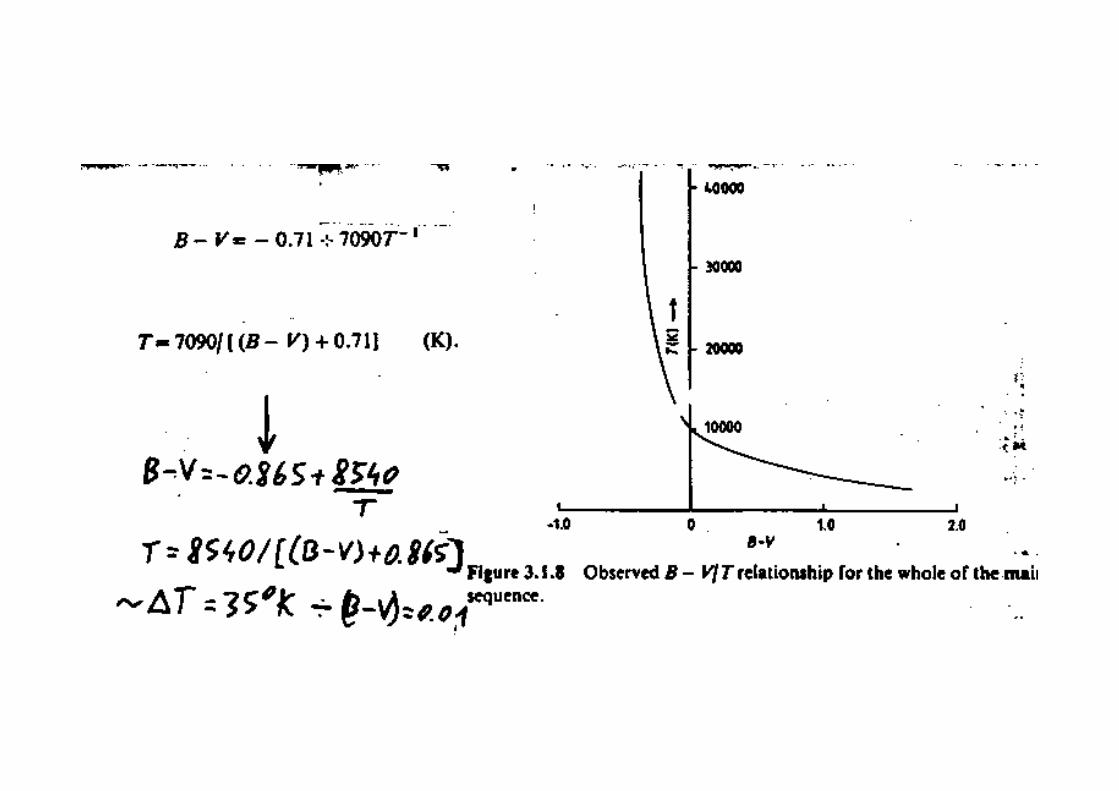
Why do we need accuratestellar photometry (1-5%) ?

Example: old star clusters, K giants

ΔV 0.1 mag. at TO~Δage 1.5 GyrΔE(B-V)=0.03 ~ ΔV 0.1 mag.

Δ(B-V)=0.03~ ΔT=100K Δ[Fe/H]~0.07, Δ[Ca/Fe]~0.1 ! Absolute calibration required

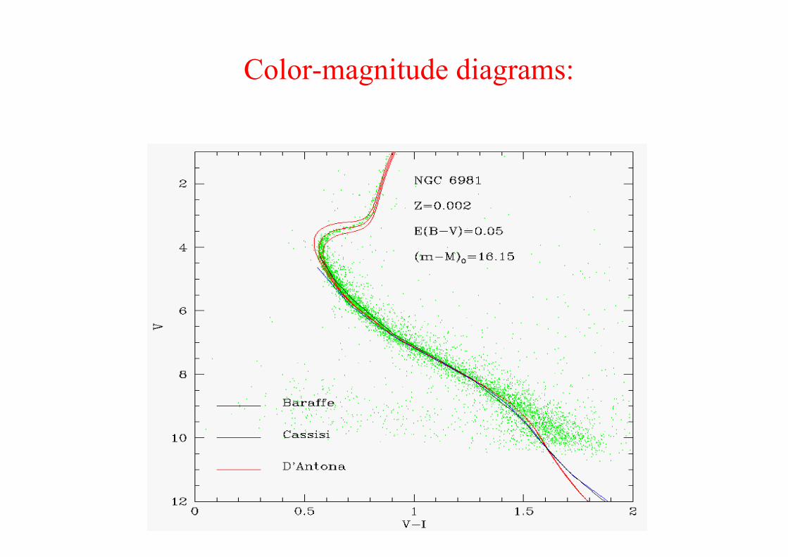
Color-magnitude diagrams:

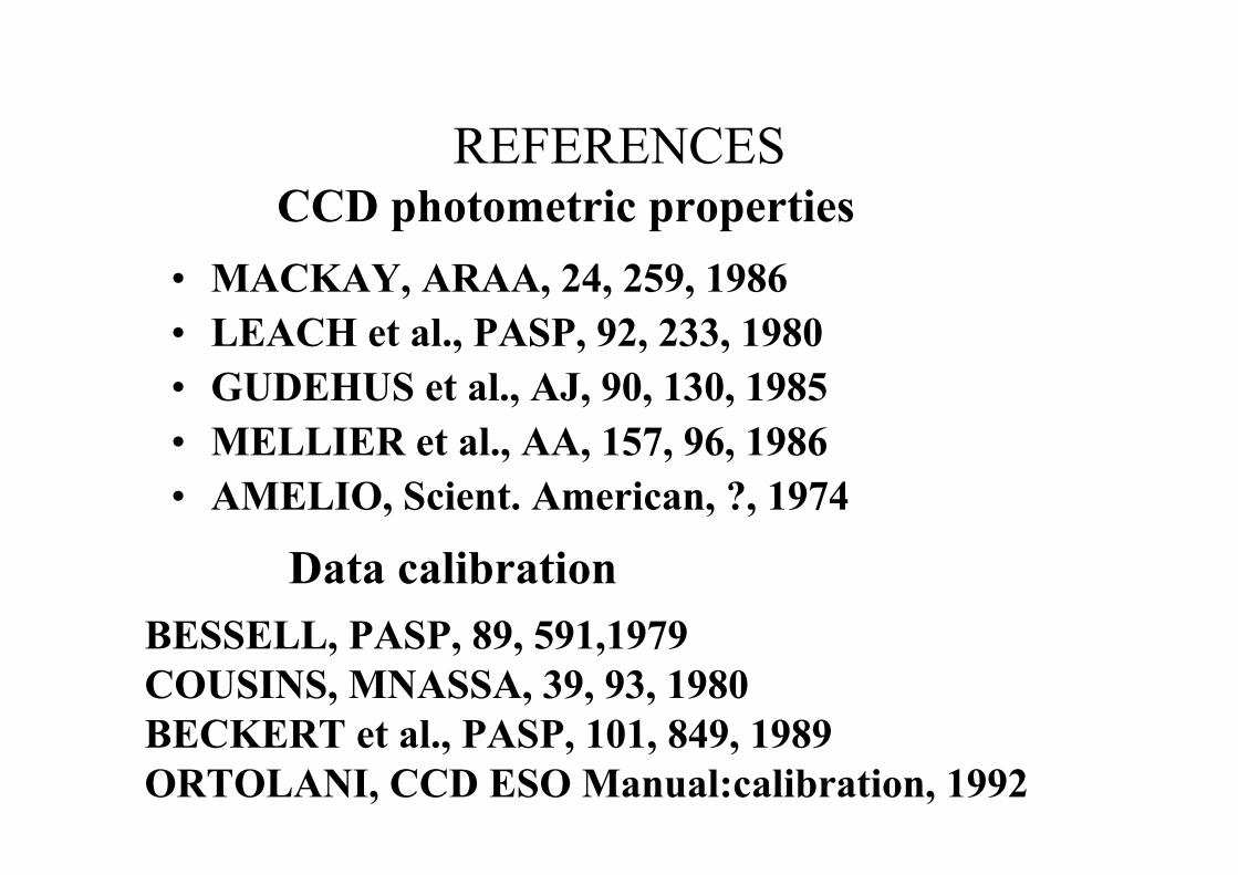
REFERENCES

• MACKAY, ARAA, 24, 259, 1986• LEACH et al., PASP, 92, 233, 1980• GUDEHUS et al., AJ, 90, 130, 1985• MELLIER et al., AA, 157, 96, 1986• AMELIO, Scient. American, ?, 1974

CCD photometric properties

Data calibrationBESSELL, PASP, 89, 591,1979COUSINS, MNASSA, 39, 93, 1980BECKERT et al., PASP, 101, 849, 1989ORTOLANI, CCD ESO Manual:calibration, 1992

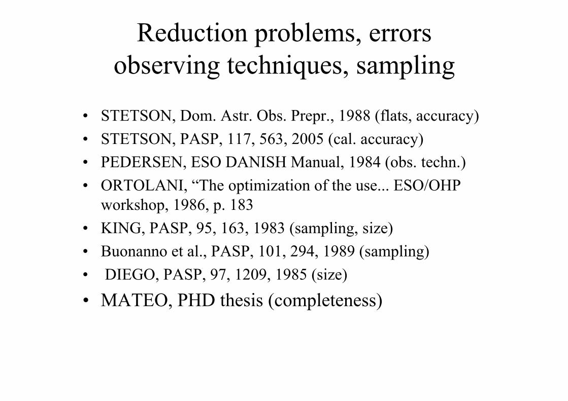
Reduction problems, errorsobserving techniques, sampling

• STETSON, Dom. Astr. Obs. Prepr., 1988 (flats, accuracy)• STETSON, PASP, 117, 563, 2005 (cal. accuracy)• PEDERSEN, ESO DANISH Manual, 1984 (obs. techn.)• ORTOLANI, “The optimization of the use... ESO/OHP

workshop, 1986, p. 183• KING, PASP, 95, 163, 1983 (sampling, size)• Buonanno et al., PASP, 101, 294, 1989 (sampling)• DIEGO, PASP, 97, 1209, 1985 (size)• MATEO, PHD thesis (completeness)

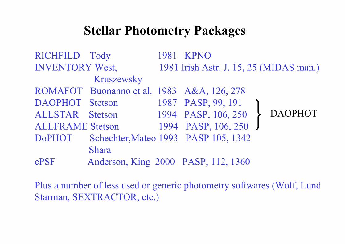
Stellar Photometry Packages

RICHFILD Tody 1981 KPNOINVENTORY West, 1981 Irish Astr. J. 15, 25 (MIDAS man.) KruszewskyROMAFOT Buonanno et al. 1983 A&A, 126, 278DAOPHOT Stetson 1987 PASP, 99, 191ALLSTAR Stetson 1994 PASP, 106, 250 ALLFRAME Stetson 1994 PASP, 106, 250DoPHOT Schechter,Mateo 1993 PASP 105, 1342 SharaePSF Anderson, King 2000 PASP, 112, 1360

Plus a number of less used or generic photometry softwares (Wolf, LundStarman, SEXTRACTOR, etc.)

DAOPHOT

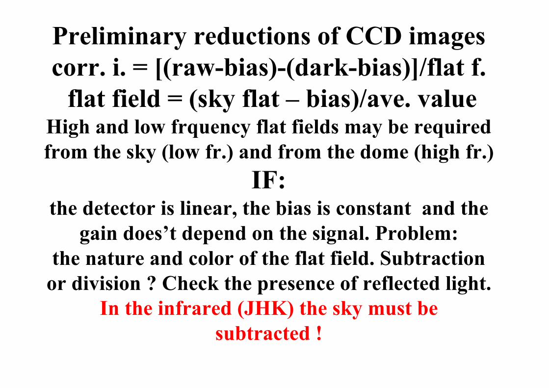
Preliminary reductions of CCD imagescorr. i. = [(raw-bias)-(dark-bias)]/flat f. flat field = (sky flat – bias)/ave. value

High and low frquency flat fields may be requiredfrom the sky (low fr.) and from the dome (high fr.)

IF:the detector is linear, the bias is constant and the

gain does’t depend on the signal. Problem:the nature and color of the flat field. Subtraction

or division ? Check the presence of reflected light.In the infrared (JHK) the sky must be

subtracted !

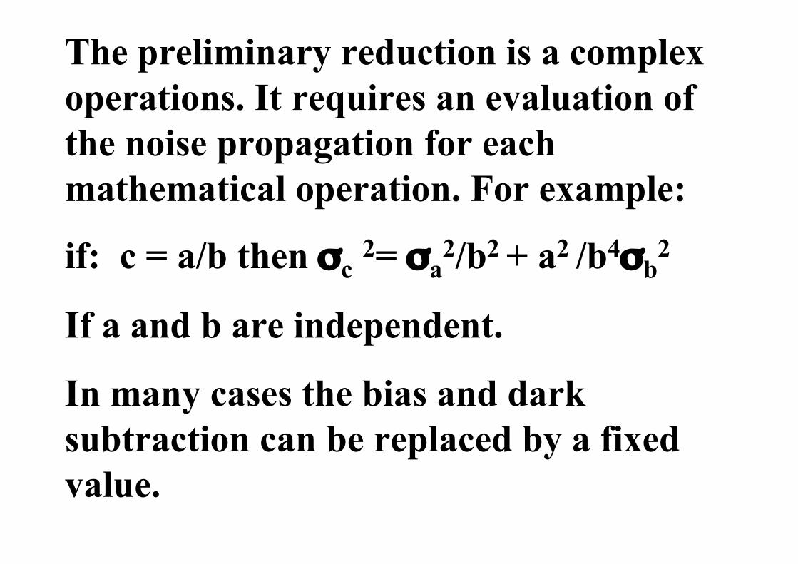
The preliminary reduction is a complexoperations. It requires an evaluation ofthe noise propagation for eachmathematical operation. For example:

if: c = a/b then σc 2= σa2/b2 + a2 /b4σb

2

If a and b are independent.

In many cases the bias and darksubtraction can be replaced by a fixedvalue.

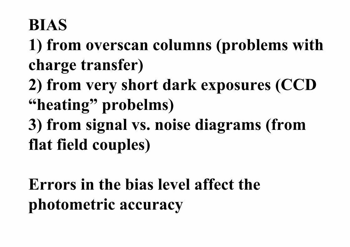
BIAS1) from overscan columns (problems with charge transfer)2) from very short dark exposures (CCD“heating” probelms)3) from signal vs. noise diagrams (from flat field couples)

Errors in the bias level affect the photometric accuracy

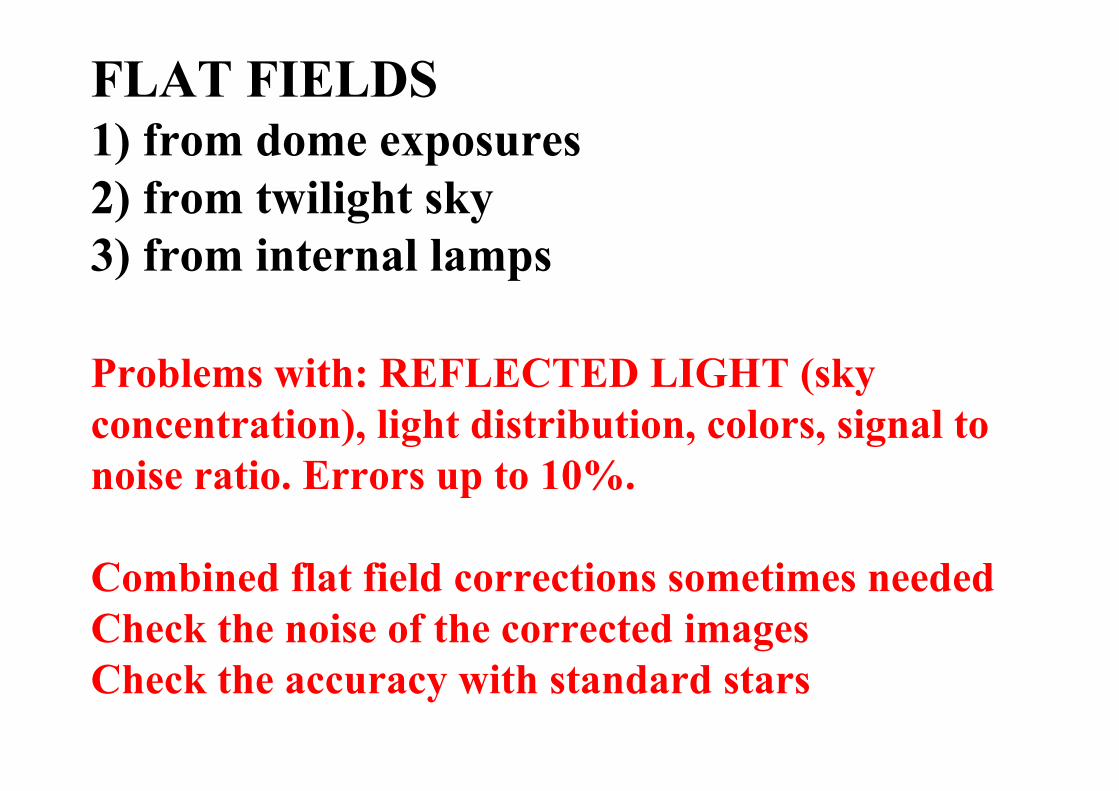
FLAT FIELDS 1) from dome exposures2) from twilight sky3) from internal lamps

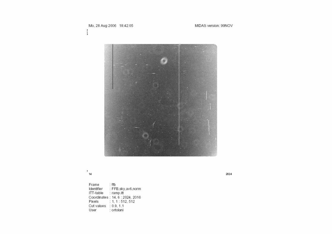
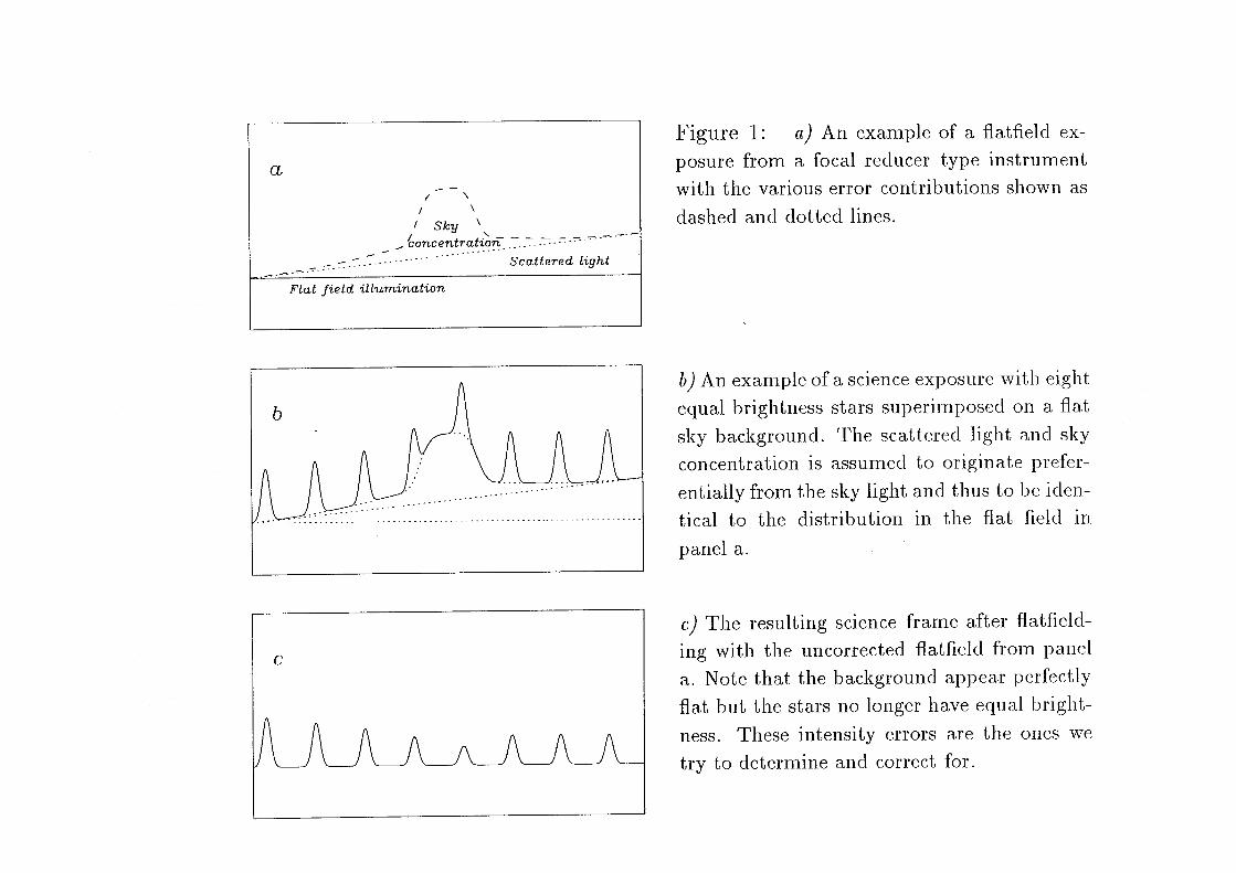
Problems with: REFLECTED LIGHT (sky concentration), light distribution, colors, signal to noise ratio. Errors up to 10%.

Combined flat field corrections sometimes neededCheck the noise of the corrected imagesCheck the accuracy with standard stars

Effect of the flat field corrections on the noise of a image.

The noise decreases with the scale length because of thebigger sampling.

From Leach et al. 1980.

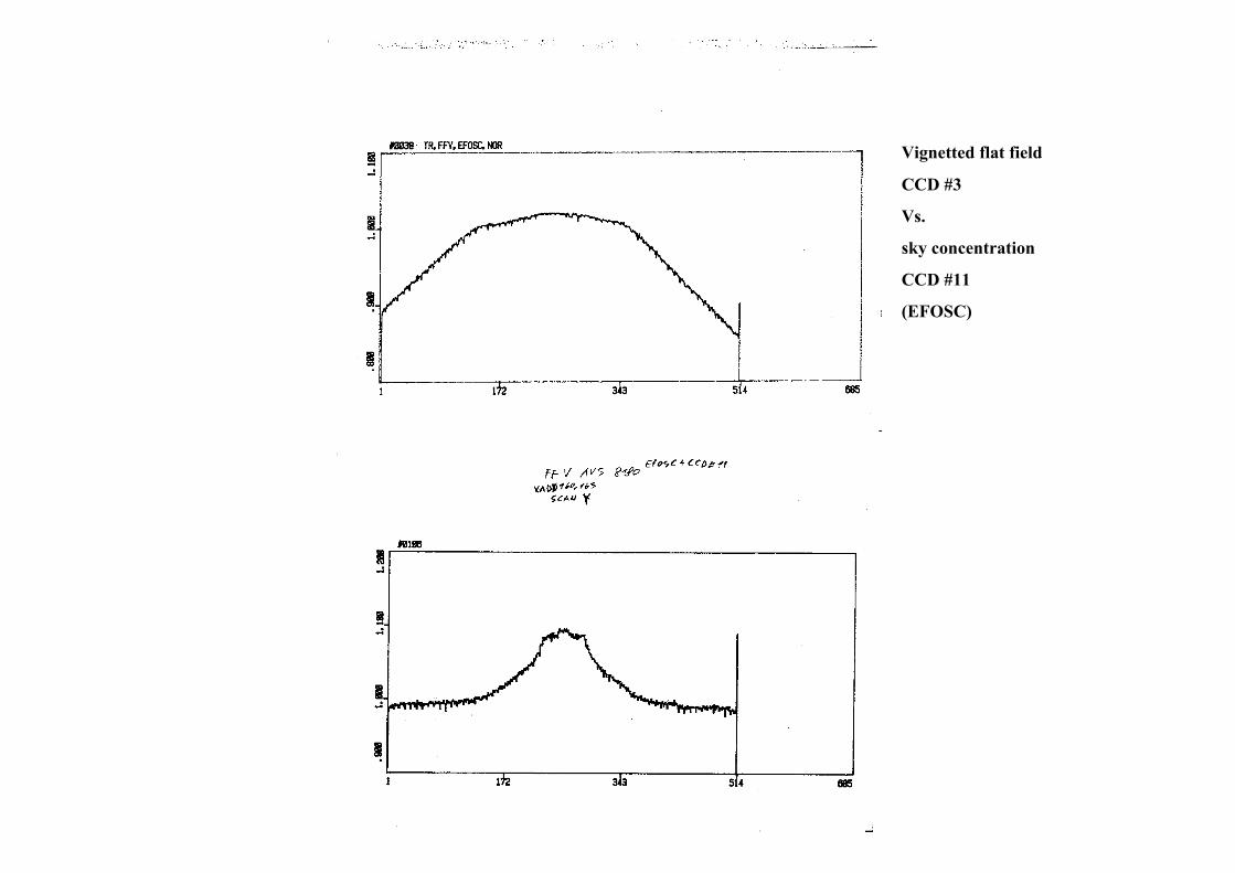
Vignetted flat field

CCD #3

Vs.

sky concentration

CCD #11

(EFOSC)

Photometric calibration, standard stars out of the field

Problems: different photometric systems, red leaks, seeing variations, air mass corrections, shutter timing, aperture corrections, sky transmissionvariations (also sky brightness fluctuations in the IR).Calibration errors +/-0.01 - 0.02 mag.

It is important to realize that, even if the filters are properly selectedany observational system is always different from the standard one.Indeed, the collected flux depends on at least 6 different terms:

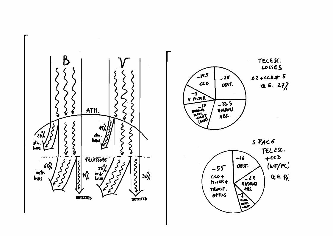
Signal=F(λ)(1-ε)R(λ)A(λ)K(λ)Q(λ)

F(λ) incoming flux A(λ) atmospheric absorptionε fraction of the obscured mirror K(λ) filter trasmission curveR(λ) mirror reflectivity Q(λ) detector quantum efficency

In the case of CCD photometry the different Q(λ) is responsible forsignificative differences, including red leaks.

Red leakage

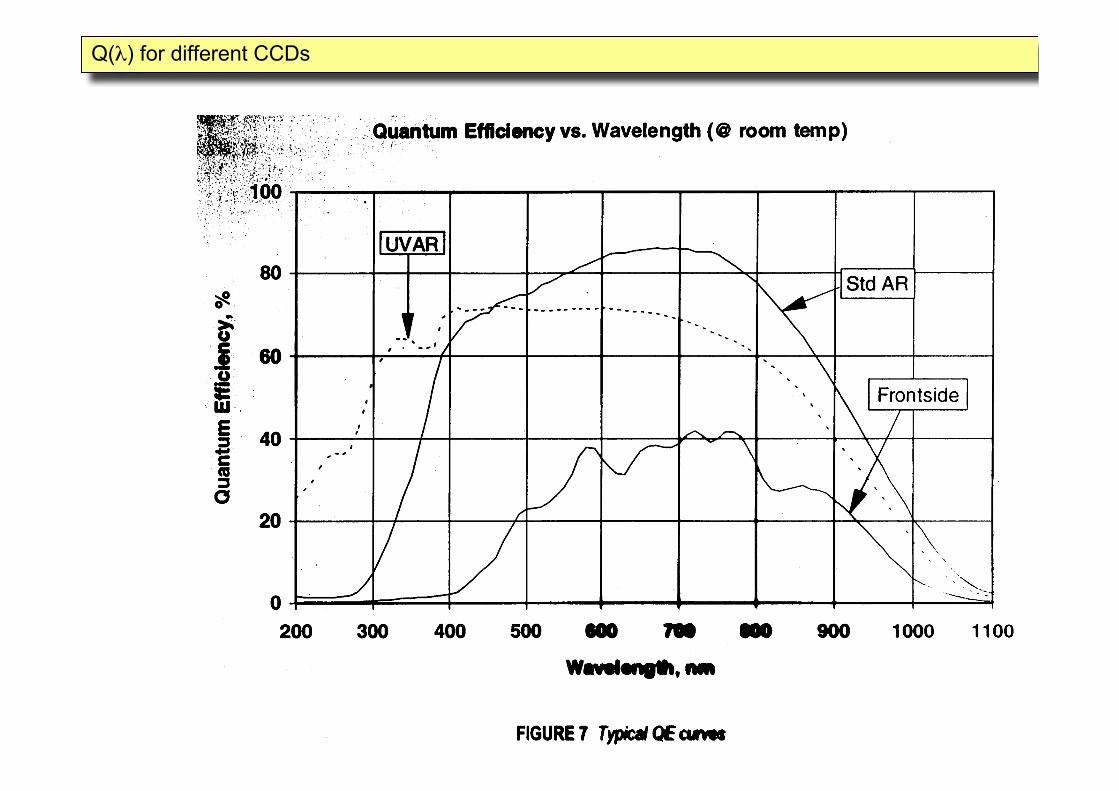
Q(λ) for different CCDs

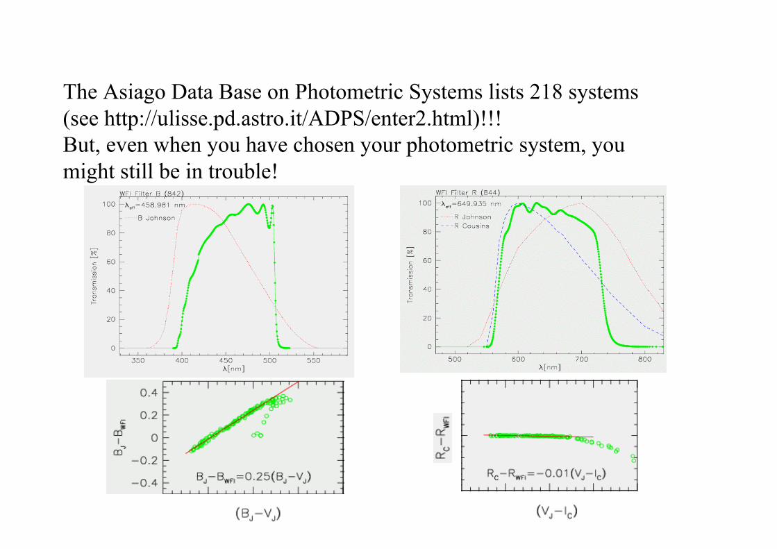
The Asiago Data Base on Photometric Systems lists 218 systems (see http://ulisse.pd.astro.it/ADPS/enter2.html)!!!But, even when you have chosen your photometric system, youmight still be in trouble!

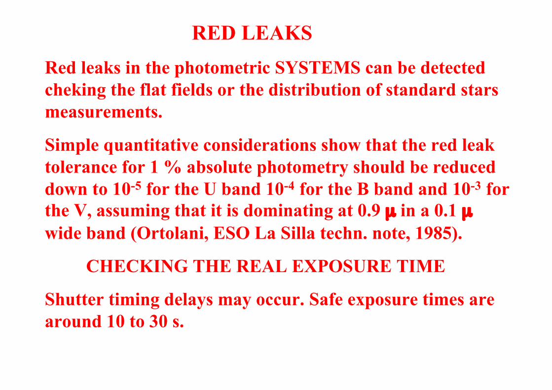
RED LEAKSRed leaks in the photometric SYSTEMS can be detectedcheking the flat fields or the distribution of standard starsmeasurements.

Simple quantitative considerations show that the red leaktolerance for 1 % absolute photometry should be reduceddown to 10-5 for the U band 10-4 for the B band and 10-3 forthe V, assuming that it is dominating at 0.9 µ in a 0.1 µwide band (Ortolani, ESO La Silla techn. note, 1985).

CHECKING THE REAL EXPOSURE TIME

Shutter timing delays may occur. Safe exposure times arearound 10 to 30 s.

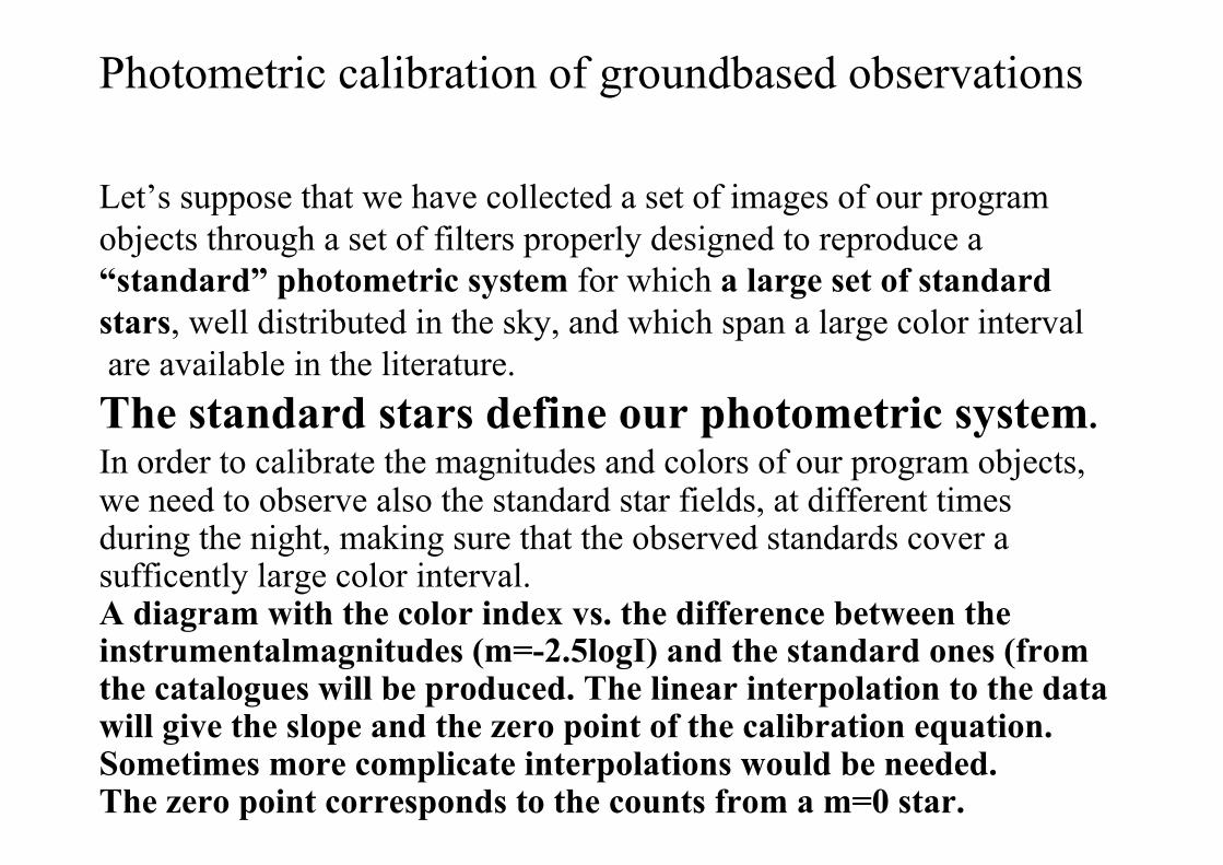
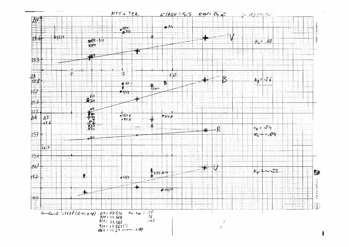
Photometric calibration of groundbased observations

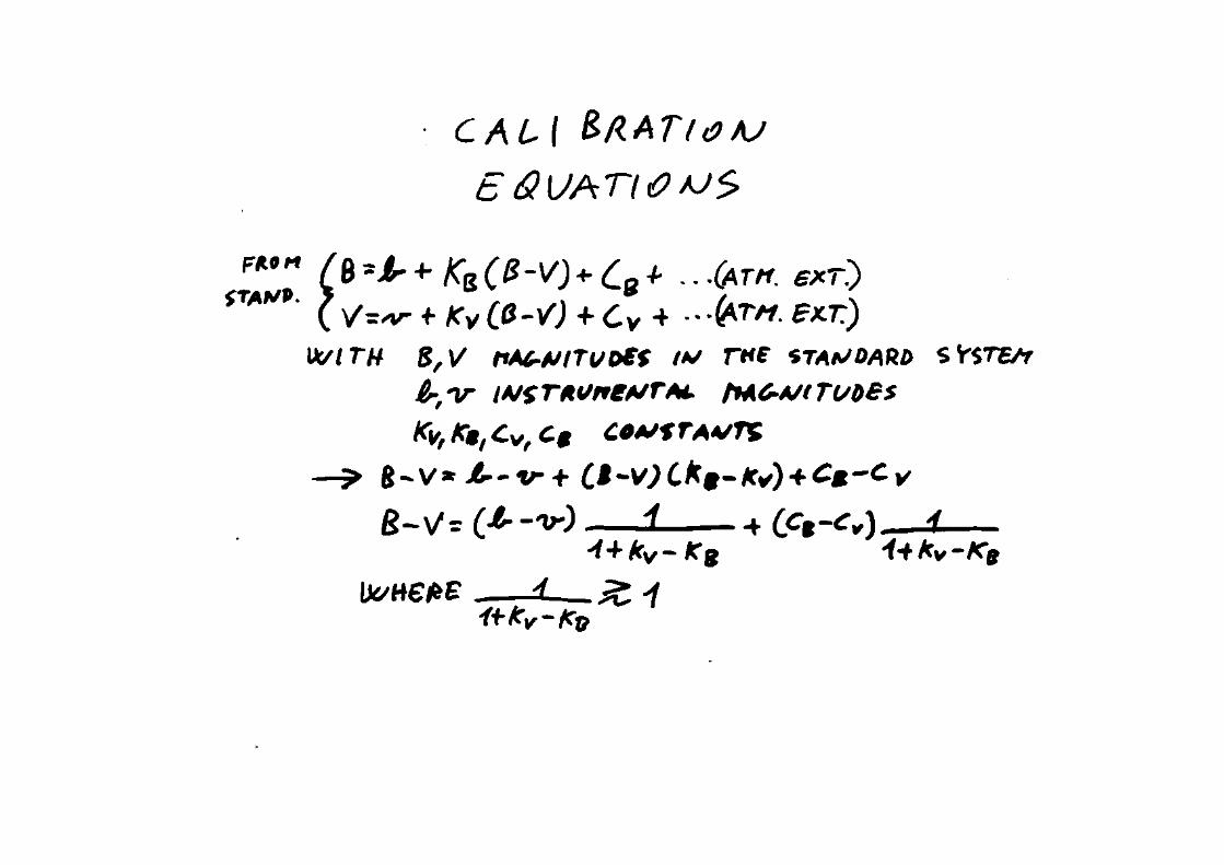
Let’s suppose that we have collected a set of images of our programobjects through a set of filters properly designed to reproduce a“standard” photometric system for which a large set of standardstars, well distributed in the sky, and which span a large color interval are available in the literature.The standard stars define our photometric system.In order to calibrate the magnitudes and colors of our program objects,we need to observe also the standard star fields, at different timesduring the night, making sure that the observed standards cover asufficently large color interval.A diagram with the color index vs. the difference between theinstrumentalmagnitudes (m=-2.5logI) and the standard ones (fromthe catalogues will be produced. The linear interpolation to the datawill give the slope and the zero point of the calibration equation.Sometimes more complicate interpolations would be needed.The zero point corresponds to the counts from a m=0 star.

Just an example (for the Johnson-Cousins system):

Landolt, 1983, AJ, 88,439Landolt, 1992, AJ, 104,340

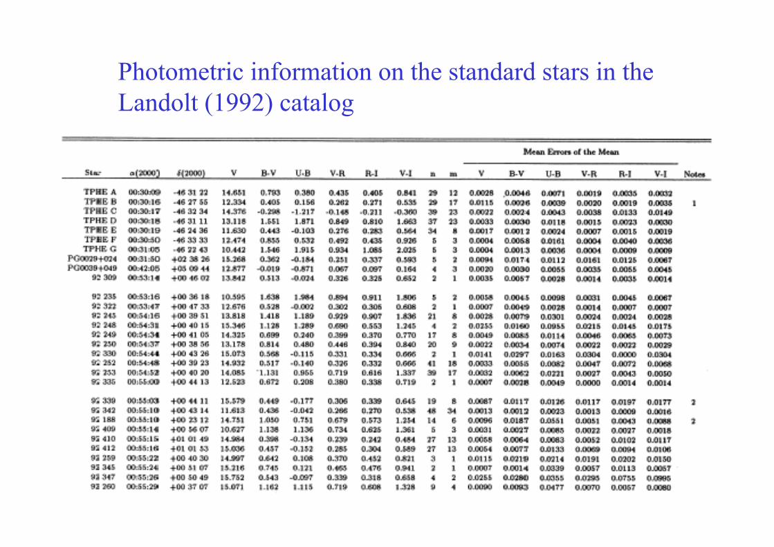
Photometric information on the standard stars in the Landolt (1992) catalog

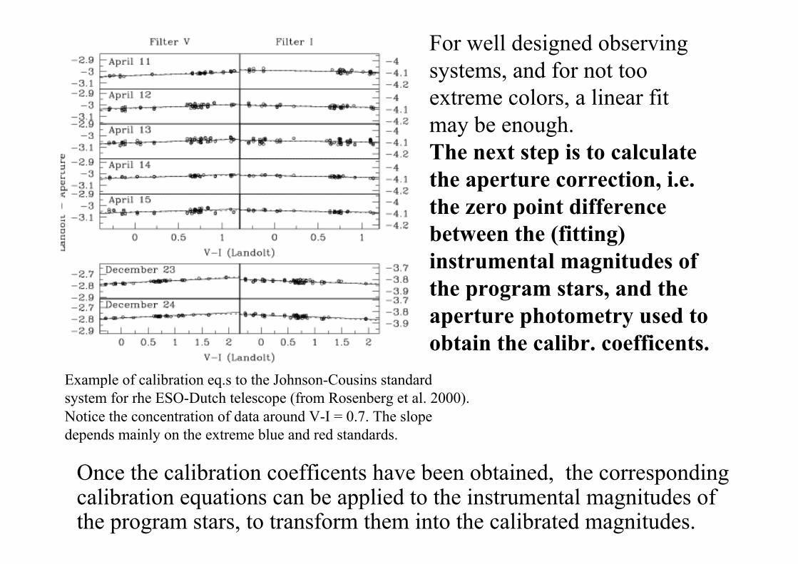
For well designed observingsystems, and for not too extreme colors, a linear fit may be enough.The next step is to calculatethe aperture correction, i.e. the zero point difference between the (fitting)instrumental magnitudes ofthe program stars, and the aperture photometry used to obtain the calibr. coefficents.

Once the calibration coefficents have been obtained, the corresponding calibration equations can be applied to the instrumental magnitudes of the program stars, to transform them into the calibrated magnitudes.

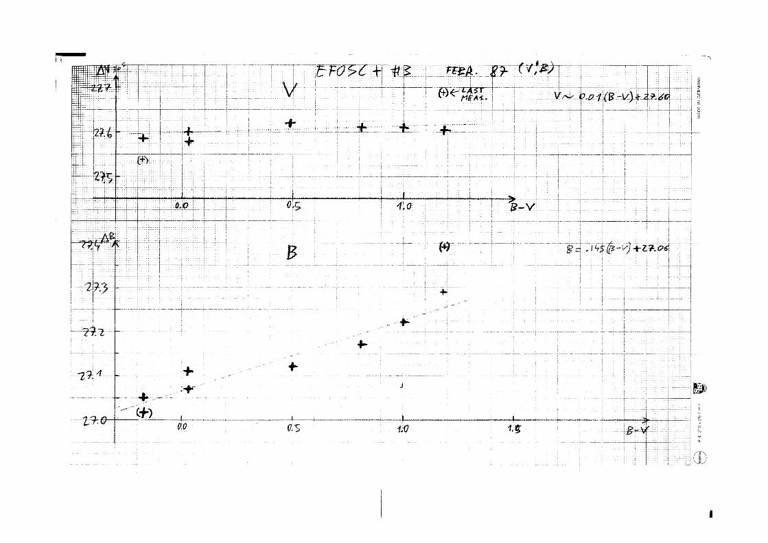
Example of calibration eq.s to the Johnson-Cousins standardsystem for rhe ESO-Dutch telescope (from Rosenberg et al. 2000).Notice the concentration of data around V-I = 0.7. The slopedepends mainly on the extreme blue and red standards.

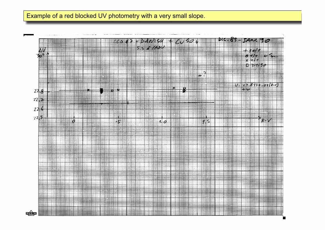
Example of a red blocked UV photometry with a very small slope.

General remarks

From the previous examples we have learned a few importantthings:

1. Observations must be calibrated and models must be transformed into the same photometric system;2. We need to use as much as possible a “standard” photometric system;3. If your photometric bandpasses are far from any existing photometric system, you have to calibrate your system starting, for example, from A0 stars (good luck!);

CONCLUSIONS

An important conclusion is that we always need to observeour objects in two bands. From a physical point of viewthis means that we need a parameter in order to define theshape of the spectrum. Then the corrections corresponding totheir spectra will be applied in order to transform their“instrumental magnitude system” into the systemdefined by the standard stars.Objects observed in a single band cannot be calibrated iftheir spectral type is not known. Possible errors are ofThe order of magnitude of the slope of the calibrationline.

HOWEVER:

1) peculiar spectra objects cannot be properly calibrated(for example multiple black body spectra, late typestars with peculiar metallicities…);

2) Very red or very blue stars are very difficult tocalibrate because there are very few good standardstars with colors below B-V=0.4 or above 1.2. Starsoutside this interval are often variables (red stars arelong period variables, blue stars are often pulsatingstars within the instability strip). The reddening shouldbe also considered because it changes the shape of thespectra. Deviations from the linear interpolation areexpected.

Recent Tests indicates errors up to 0.3 magnitudes in theV-I color from the WFI at 2.2.

SUGGESTIONS FOR AN ACCURATE CALIBRATION• CAREFULLY CHECK THE FLAT FIELDS, COMPARE SKY

AND DOME FLATS

• CHECK THE SHUTTER TIMING MEASURING IN REALTIME THE STANDARD STARS. DELAYS UP TO 0.5 sSHOULD BE EXPECTED ! THIS IS A REAL PROBLEM FORBRIGHT STARS.

• BE CAREFUL TO HAVE THE PEAK OF THE STANDARDSTARS AT LEAST 10% BELOW THE SATURATION LIMIT(50% RECOMMENDED). DEFOCUSED IMAGES GIVEMUCH MORE ACCURATE MEASUREMENTS (BUT…)

• REPEAT THE OBSERVATIONS OF THE STANDARDS,POSSIBLY INCLUDING DIFFERENT EXPOSURE TIMESAND CHANGING THEIR POSITIONS ON THE CCD, ANDMEASURE THE INSTURMENTAL MAGNITUDE IN REALTIME.

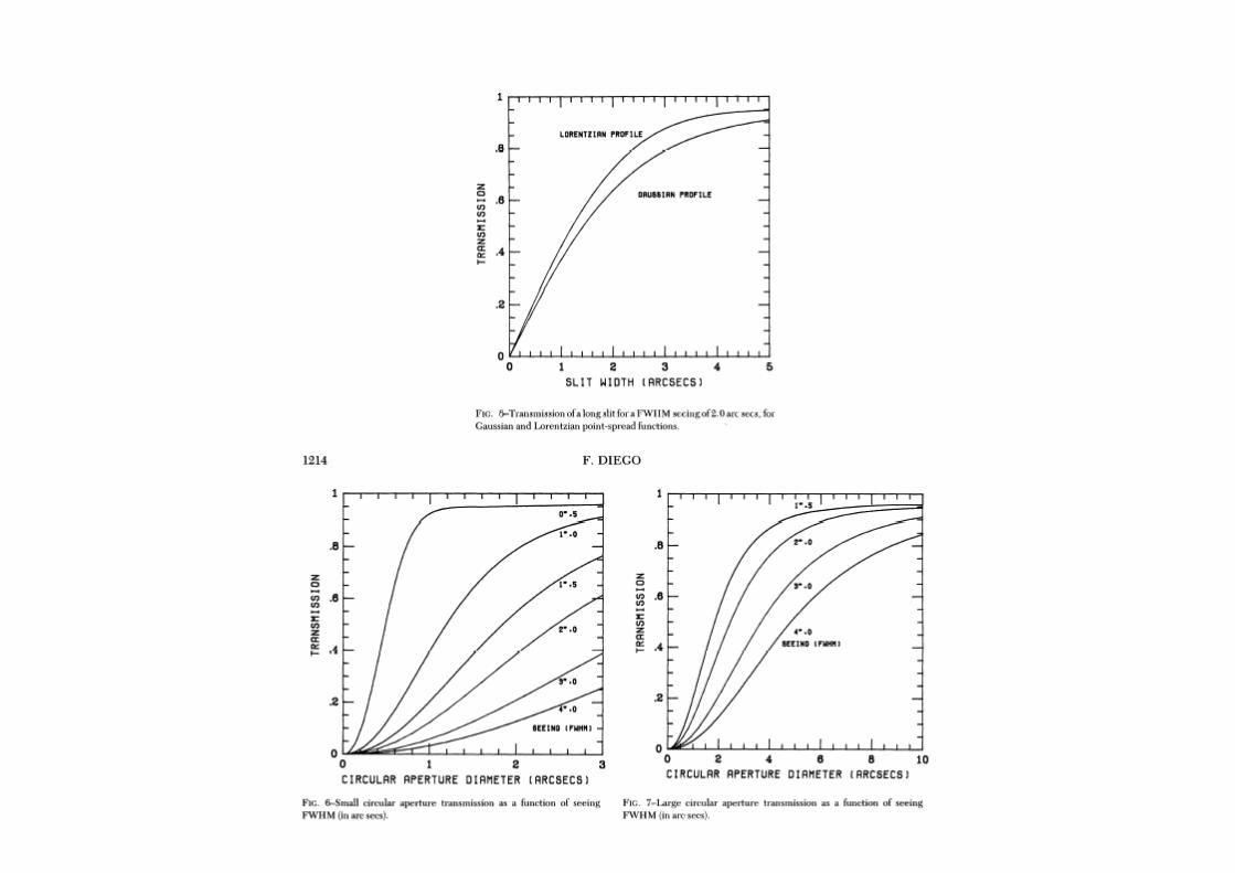
THE NEXT STEP: THE APERTURE CORRECTION

OR

HOW MUCH LIGHT OF THE STANDARD vs. OUR

STARS IN INCLUDED IN THE MEASUREMENTS ?

It could be a difficult step if:

• The standard stars have been defocused by a largeamount;

• The seeing of the standards is significantly differentfrom the stars to be calibrated

• The target stars are in very crowded fields

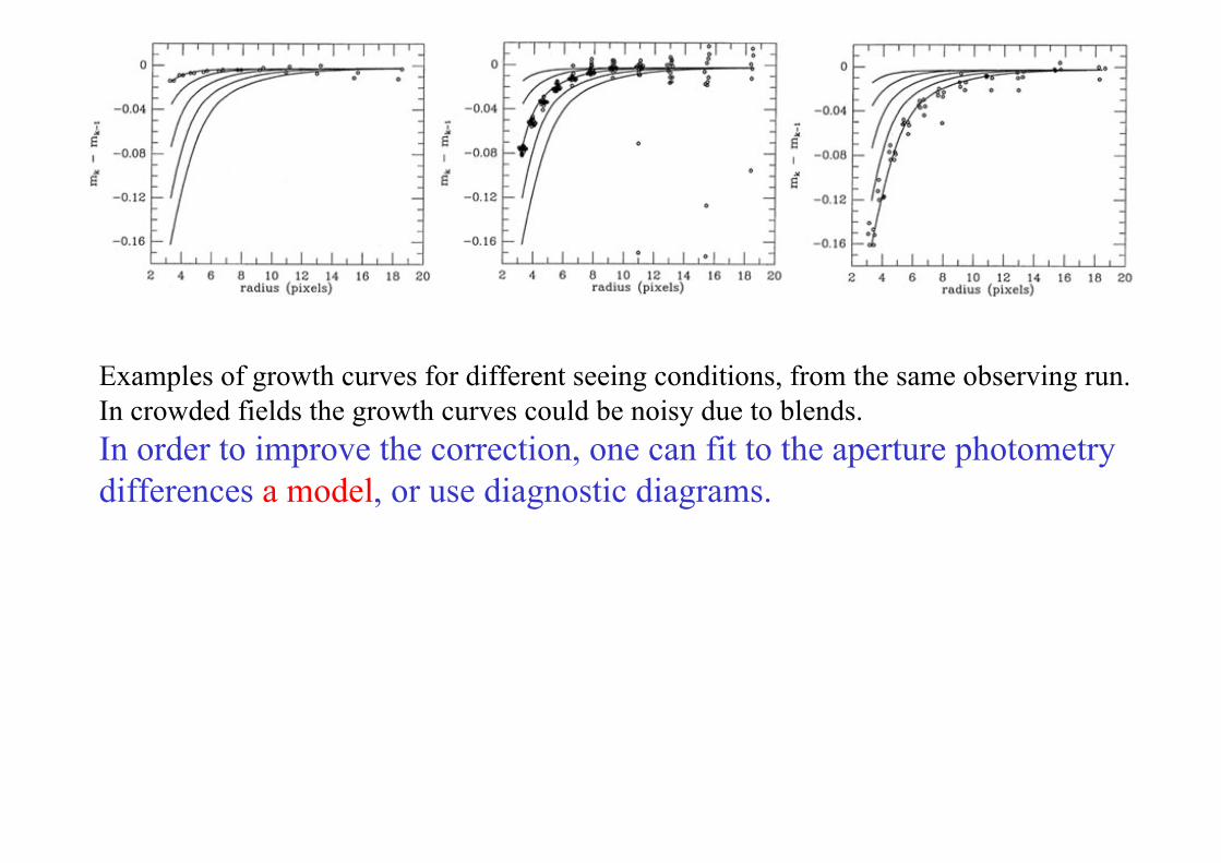
Examples of growth curves for different seeing conditions, from the same observing run.In crowded fields the growth curves could be noisy due to blends. In order to improve the correction, one can fit to the aperture photometrydifferences a model, or use diagnostic diagrams.

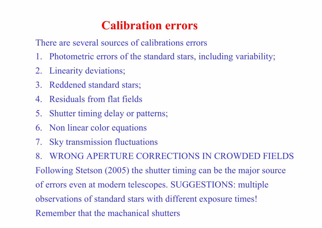
Calibration errors

There are several sources of calibrations errors

1. Photometric errors of the standard stars, including variability;

2. Linearity deviations;

3. Reddened standard stars;

4. Residuals from flat fields

5. Shutter timing delay or patterns;

6. Non linear color equations

7. Sky transmission fluctuations

8. WRONG APERTURE CORRECTIONS IN CROWDED FIELDS

Following Stetson (2005) the shutter timing can be the major source

of errors even at modern telescopes. SUGGESTIONS: multiple

observations of standard stars with different exposure times!

Remember that the machanical shutters

degrades with time.